DearFSAC: An Approach to Optimizing Unreliable Federated Learning
via Deep Reinforcement Learning
Abstract
In federated learning (FL), model aggregation has been widely adopted for data privacy. In recent years, assigning different weights to local models has been used to alleviate the FL performance degradation caused by differences between local datasets. However, when various defects make the FL process unreliable, most existing FL approaches expose weak robustness. In this paper, we propose the DEfect-AwaRe federated soft actor-critic (DearFSAC) to dynamically assign weights to local models to improve the robustness of FL. The deep reinforcement learning algorithm soft actor-critic is adopted for near-optimal performance and stable convergence. Besides, an auto-encoder is trained to output low-dimensional embedding vectors that are further utilized to evaluate model quality. In the experiments, DearFSAC outperforms three existing approaches on four datasets for both independent and identically distributed (IID) and non-IID settings under defective scenarios.
1 Introduction
With the development of mobile devices, huge quantities and diverse types of data have been generated, which promote the utilization of machine learning technologies. However, when aggregated to central model training, data with sensitive privacy can lead to serious privacy leakage. To address the privacy challenges, federated learning (FL) has been proposed to aggregate local model parameters, which are only trained on local raw data, into a global model to improve performance. In FL, mobile devices are set as clients and upload their own models to the server. As a decentralized paradigm, FL significantly reduces the risks of privacy leakage by allowing clients to access only their own raw data Zhu et al. (2018).
Although FL realizes both efficient data utilization and data privacy protection in the application of mobile networks, it is fragile when various defects affect the global model during a FL process Shayan et al. (2018), such as malicious updates, poisoning attacks Fung et al. (2018), low-quality data, and unstable network environments. Unfortunately, conventional approaches pay little attention to most defects Fung et al. (2018). Therefore, an efficient approach to alleviating performance degradation caused by defective local models is strongly needed for FL. Existing researches on blockchain-based FL have defined the concept of reputation, which manifests the reliability of each local model Kang et al. (2019) Kang et al. (2020). Similarly, we evaluate the model quality to measure how trustworthy a local model is. After learning about the quality of each local model, we are motivated to design a deep neural network (DNN) to assign optimal weights to local models, so that the global model can maintain a considerable performance no matter if there exist defects or not.
In this paper, we propose DEfect-AwaRe federated soft actor-critic (DearFSAC), a novel FL approach based on deep reinforcement learning (DRL) to guarantee a good performance of FL process by dynamically assigning optimal weights among defective local models through model quality evaluation. Since DRL algorithms often fall into local optimum, we adopt soft actor-critic (SAC) Haarnoja et al. (2018) to find near-optimal solutions for more stable performance. Besides, as unbalanced data distribution in the buffer may deteriorate the training process of the DRL model, prioritized experience replay (PER) Schaul et al. (2015) and emphasizing recent experience (ERE) Wang and Ross (2019) are employed, which are two popular importance sampling techniques. Furthermore, as local raw data is not accessible for the server, high-dimensional model parameters trained on local raw data become the only alternative uploaded and fed into the DRL model. To avoid the curse of dimensionality, we design an embedding network using the auto-encoder framework Song et al. (2013) to generate low-dimensional vectors containing model-quality features.
In summary, the main contributions of this paper are as follows:
-
1.
As far as we know, we are the first to propose the approach that dynamically assigns weights to local models under defective scenarios based on DRL.
-
2.
We design an auto-encoder based on network embedding techniques Cui et al. (2018) to evaluate the quality of local models. This module also accelerates the DRL training process.
-
3.
The experimental results show that DearFSAC outperforms existing approaches and achieves considerable performance while encountering defects.
2 Preliminaries
2.1 Federated Learning
Suppose we have one server and clients whose data is sampled from the local raw dataset . The model parameters of the th client and the server are denoted as and at round respectively, where is the total parameter number of one model. Then, the objective of clients is converted into an empirical risk minimization Yang et al. (2019) as follows:
| (1) |
| (2) |
where is downloaded from the server by clients, and represents the loss of on the local data sampled from . For the server, the objective is to find the optimal global model parameters:
| (3) |
2.2 Deep Reinforcement Learning
In DRL, an agent, which is usually in a DNN form, interacts with the environment by carrying out actions and obtaining rewards. The whole process can be modelled as a Markov decision process (MDP) Sutton and Barto (2018), defined by , in which denotes a set of states and denotes a set of actions. is the state transition function used to compute the probability of the next state given current action and current state . The reward at time step is computed by the reward function and future rewards are discounted by the factor .
At each time step , the agent observes the state , and then interacts with environment by carrying out an action sampled from the policy which is a distribution of given . After that, the agent obtains a reward and observes the next state . The goal is to find an optimal policy which maximizes the cumulative return: .
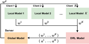
In this paper, SAC algorithm is adopted, which is an algorithm to optimize using actor-critic algorithm Konda and Tsitsiklis (2000) and entropy regularization Nachum et al. (2017). Through the DRL model, the server in FL assigns optimal weights to clients. The structure of FL combined with DRL is illustrated in Fig. 1.
3 Methodology
In this section, we discuss the details of DearFSAC, a DRL-based approach to assigning optimal weights to defective local models in FL. In Section 3.1, we describe the entire process of our approach. In Section 3.2, we design the quality evaluation embedding network (QEEN) for dimension reduction and model quality evaluation. In Section 3.3, we adopt SAC to optimize , which gets more stable convergence and more sufficient exploration than other actor-critic algorithms.
3.1 Overall Architecture of DearFSAC
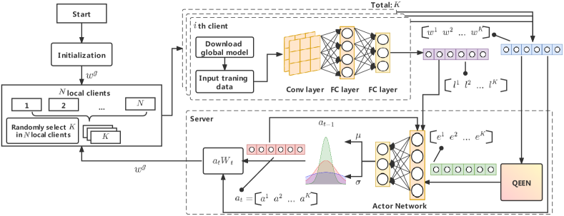
The overall architecture of DearFSAC is shown in Fig. 2. At the first round, the global model parameters and the DRL action are randomly initialized. Then all clients train their own models locally and of them are randomly selected to upload model parameters and local training loss . After receiving uploaded information, the server feeds the local model parameters into QEEN and gets the embedding vectors . Next, the embedding vectors, local losses, and the last action are concatenated and fed into the actor network of the DRL model to get the current action . Finally, by using , the server aggregates local model parameters to the global model parameters and shares with all clients. The whole process loops until convergence.
3.2 Dimension Reduction and Quality Evaluation
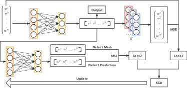
Based on an auto-encoder structure, QEEN is designed for both dimension reduction and quality evaluation. At round , for training efficiency, we upload all local model parameters to the server and add several types of defects into half of them. Then we design loss for the embedding of and loss Hastie et al. (2009) for quality evaluation. The auto-encoder on the server receives model parameters as training data and performs training using both and .
We feed each into the encoder composed of two fully connected (FC) layers and get the embedding vector of the th model:
| (4) |
After obtaining all embedding vectors, we put into the decoder to produce a decoded representation which approximates . Different from conventional ways of auto-encoder, we adopt network embedding Wang et al. (2016) and design the decoder into parallel FC layers , where is the number of layers of the original model, is the th parallel FC layer corresponding to the th layer of the original model structure Zinkevich et al. (2010), where . Next, for the th model, the embedding vector is fed into the th parallel layer to get decoded layer parameters of the original model:
| (5) |
and concatenate each layer by layer to obtain the entire decoded model parameters:
| (6) |
After getting , we use mean square error (MSE) loss function to compute :
| (7) |
As multiple defects have different impact on local models, we define defect marks as the ground truth, denoted as , where is the degree of defect. Next, we compare defect marks with quality evaluation marks . We feed into the quality evaluation module composed of two FC layers to get to predict the quality of the th model:
| (8) |
Then we compute :
| (9) |
Finally, we set different weights and for two kinds of loss, generally and respectively, to update the QEEN parameter using joint gradient descent Tanaka et al. (2018) as follows:
| (10) |
The entire training process of QEEN is illustrated in Fig. 3.
3.3 DRL for Optimal Weight Assignment
3.3.1 MDP Modelling:
To guarantee the communication efficiency and fast convergence, clients are randomly selected among the clients at each round and upload models to the server. After receiving various information as the current state, the DRL model outputs an action containing weights of all selected models. The details and explanations of , , and are defined as follows:
State : At round , the state can be denoted as a vector , where denotes the embedding vector of th client’s model parameters, denotes the embedding vector of the server’s model parameters, denotes the local training loss of th local model, and denotes the action at the last round.
Action : The action, denoted as , is a weight vector calculated by the DRL agent for randomly selected subset of model parameters at round . All the weights in are within and satisfy the constraint . After obtaining the weight vectors, the server aggregates local model parameters to the global model as follows:
| (11) |
where is a set of all selected local models.
Reward : The goal of DRL is to maximize cumulative reward in total time steps , which is equivalent to finding the local model with minimum loss shown in Eq. (1). Therefore, we design a compound reward by combining three sub-rewards with appropriate weights , which can be formulated as:
| (12) | ||||
| (13) | ||||
| (14) |
| (15) | ||||
In Eq. (13), is defined within to maximize global model’s accuracy. The exponential term and represent the accuracy gap, where is the global model’s accuracy on the held-out validation set at round , is the target accuracy which is usually set to , and is the accuracy of the model aggregated by FedAvg. is a positive constant to ensure an exponential growth of . As is in , the second term, , is used as time penalty at each round to set to for faster convergence.
3.3.2 Adopting SAC to Solve MDP:
First, locally trained models are randomly selected to upload the parameters and local loss to the server. Through QEEN, we can obtain embedding vectors as part of the current state . By feeding into the actor network, we obtain the current action . After model aggregation, we get reward and the next state . Empirically, we set as . At the end of each round, the tuple , which is denoted as , is recorded in the buffer.
For each iteration, SAC samples a batch of from the buffer and updates the DRL network parameters. To deal with poor sampling efficiency and data unbalance in DRL, we adopt two techniques of replay buffer named ERE Wang and Ross (2019) and PER Schaul et al. (2015) to sample data with priority and emphasis. For the th update, we sample data uniformly from the most recent data points , defined as:
| (16) |
where represents the degree of emphasis on recent data and is the maximum size of buffer . After obtaining an emphasizing buffer according to , the sampling probability of data point in PER is computed as:
| (17) |
where is a hyperparameter determining the affection of the priority, is a hyperparameter controlling the affection of . in Eq. (17) is the priority value of the th data point, defined as:
| (18) |
where is the bias and is the action-value function formulated as:
| (19) |
where is the entropy of , formulated as:
| (20) |
Next, we compute the importance sampling weight of the th data point as:
| (21) |
After sampling , SAC Haarnoja et al. (2018) updates the DRL model and aims to find to maximize both the total reward and the entropy, which leads to more stable convergence and more sufficient exploration:
| (22) |
where is a trade-off coefficient.
4 Experiments
In this section, we conduct various experiments to validate the performance of DearFSAC on defective local models. Specially, we compare the test accuracy of DearFSAC with different approaches on four datasets in Section 4.2. Then, we try different numbers of defective models and degrees of defect to show robustness of DearFSAC in Section 4.3. Besides, in Section 4.4, we discuss the effectiveness of QEEN by designing ablation experiments.
4.1 Experimental Setup
4.1.1 Datasets
We validate the proposed DRL model on four datasets: MNIST LeCun et al. (1998), CIFAR-10 Krizhevsky et al. (2009), KMNIST Clanuwat et al. (2018), and FashionMNIST Xiao et al. (2017). For convenience, we call the three MNIST datasets X-MNIST. The setup is illustrated in Table 1, The X-MNIST datasets contain both IID and non-IID data while the CIFAR-10 dataset contains only IID data.
| Parameter | X-MNIST | CIFAR-10 | |
|---|---|---|---|
| IID | NonIID | IID | |
| Total Clients | 100 | 100 | 100 |
| Selection Number | 10 | 10 | 10 |
| Model Size | 26474 | 26474 | 62006 |
4.1.2 Defect Types
We define the number of defective models as and the degree of defect as . Then we design three types of defect:
-
•
Data contamination: We add standard Gaussian noise to each pixel in an image and obtain defective pixels .
-
•
Communication Loss: We add standard Gaussian noise to each parameter in the last two layers and obtain defective parameters .
-
•
Malicious attack: For both IID and non-IID datasets, we shuffle labels of each local training batch.
4.1.3 Metrics
To evaluate the performance of DearFSAC and compare it with other weight assignment approaches, we mainly identify three performance metrics as follows:
-
•
: The averaging accuracy on test datasets over multiple times.
-
•
: The number of communication rounds to first achieve in corresponding datasets.
-
•
: The cumulative reward of DRL approaches in each episode.
4.2 Comparisons across Different Datasets
In this subsection, we compare our approach with FedAvg, rule-based strategy, and supervised learning (SL) model. For rule-based strategy, it assigns weights to models with no defects. For SL model Cui et al. (2018), it consists of FC layers with and units and performs training with defect marks. We compose three types of defects at the same time to obtain the composite defect. Then we adopt it in both DRL training process and FL test. We conduct experiments on the FL training dataset for rounds, setting and .
As shown in Table 2, we carry out 100-round FL training process for ten times and compare and of each approach. The results on the IID datasets show that our approach significantly outperforms the other three approaches in all four IID datasets. Furthermore, we compare our approach with FedAvg with no defect in local models and find that our approach performs almost the same as FedAvg in the defectless setting. This is because the data distribution is IID so that averaging weights is a near-optimal strategy, which exhibits that our approach converges to FedAvg in the simplest setting.
On the other hand, our approach also performs the best on non-IID datasets. As data distribution is largely different, of each approach decreases obviously, especially the rule-based strategy and SL model. In non-IID KMNIST, the performance of rule-based strategy is similar to that of FedAvg. These two results show that fixed weight is not feasible in non-IID datasets. Besides, FedAvg with no defects needs more communication rounds on non-IID datasets than DearFSAC, which shows the advantage in speed of DearFSAC.
All the above results show that our approach performs the best no matter whether there exist defects in local models or not, which verify the generalization of our approach.
| Approach | MNIST | KMNIST | FashionMNIST | CIFAR | |||
|---|---|---|---|---|---|---|---|
| IID | Non-IID | IID | Non-IID | IID | Non-IID | IID | |
| DearFSAC-nodefect | 97.45%/7 | 94.64%/20 | 89.03%/39 | 76.52%/35 | 85.06%/44 | 73.98%/23 | 58.29%/40 |
| DearFSAC | 98.06%/7 | 95.29%/19 | 88.69%/40 | 77.2%/36 | 85.59%/43 | 73.47%/21 | 57.21%/41 |
| FedAvg-nodefect | 97.57%/11 | 95.07%/20 | 88.23%/42 | 75.30%/39 | 85.43%/44 | 71.69%/26 | 57.37%/41 |
| FedAvg | 62.76%/- | 39.26%/- | 42.65%/- | 28.72%/- | 33.61%/- | 22.55%/- | 28.15%/- |
| Rule-based | 85.27%/- | 69.37%/- | 72.78%/- | 31.29%/- | 68.17%/- | 26.67%/- | 47.93%/- |
| SL | 86.20%/- | 75.88%/- | 78.97%/- | 39.83%/- | 69.51%/- | 28.91%/- | 51.57%/- |
4.3 Defect Impact
In this subsection, we compare the performance of the above approaches on non-IID MNIST to study the impact of different and .
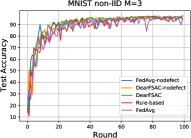
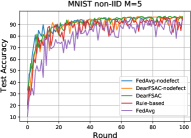

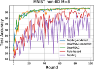
First, we change the value of to study how the numbers of defective models impact the performance. Fig. 4 shows that as increases, the accuracy decreases dramatically. When is small, defects cause little impact on the global model. On the contrary, if is relatively larger, it becomes sensitive to accuracy of the global model. It also shows that FL has limited capability to resist defects. Compared with FedAvg, our approach has a more robust performance despite large .
| Approach | ||||
|---|---|---|---|---|
| DearFSAC | FedAvg | Rule-based | SL | |
| 0.1 | 94.64% | 35.26% | 69.37% | 75.88% |
| 0.3 | 94.91% | 19.64% | 68.21% | 71.62% |
| 0.5 | 94.27% | 12.73% | 68.77% | 63.83% |
| 0.7 | 93.87% | 10.33% | 70.05% | 53.11% |
| 0.9 | 95.06% | 9.55% | 69.56% | 42.65% |
In Table 3, we study how the degree of the composite defect affects the performance. As increases, the accuracy of FedAvg decreases dramatically while our approach holds a high and stable accuracy, which indicates that the accuracy of the global model is quite sensitive to .
All the above experiments show that our approach is capable of adapting multiple numbers and degrees of composite defect, validating the robustness of our approach.
4.4 Effectiveness of QEEN
In this subsection, we study the effectiveness of QEEN by comparing the cumulative reward and the accuracy of DearFSAC with that of original SAC and embedding SAC, where embedding SAC adopts only an embedding network for dimension reduction. We compare the three versions of DRL model on IID and non-IID MNIST datasets. Here we set , where total episodes is and each episode contains rounds.
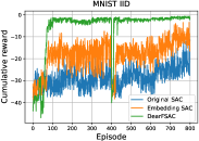
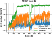
4.4.1 Cumulative Reward
In Fig. 5, for IID MNIST and non-IID MNIST, of DearFSAC increases rapidly at the beginning and gradually converges, while of embedding SAC fluctuates dramatically, which indicates that quality evaluation not only largely improves the accuracy, but also guarantees the convergence speed and stability in DearFSAC. Besides, of original SAC is the worst which means that embedding network also matters in DearFSAC for good performance.
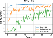
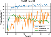
4.4.2 Accuracy
In Fig. 6, the test accuracy of DearFSAC is significantly higher than the original SAC and embedding SAC, which again proves our conclusions.
5 Conclusion and Future Work
In this paper, we propose DearFSAC, which assigns optimal weights to local models to alleviate performance degradation caused by defects. For model quality evaluation and dimension reduction, an auto-encoder named QEEN is designed. After receiving embedding vectors generated from QEEN, the DRL agent optimizes the assignment policy via SAC algorithm. In the experiments, we evaluate the performance of DearFSAC on four image datasets in different settings. The results show that DearFSAC outperforms FedAvg, rule-based strategy, and SL model. Specially, our model exhibits high accuracy, stable convergence, and fast training speed no matter whether there exist defects in FL process or not.
In the future, it is worthwhile investigating how to extend DearFSAC to a multi-agent framework for personalized FL in defective situations.
References
- Clanuwat et al. [2018] Tarin Clanuwat, Mikel Bober-Irizar, Asanobu Kitamoto, Alex Lamb, Kazuaki Yamamoto, and David Ha. Deep learning for classical japanese literature. arXiv preprint arXiv:1812.01718, 2018.
- Cui et al. [2018] Peng Cui, Xiao Wang, Jian Pei, and Wenwu Zhu. A survey on network embedding. IEEE Transactions on Knowledge and Data Engineering, 31(5):833–852, 2018.
- Dehak et al. [2010] Najim Dehak, Reda Dehak, James R Glass, Douglas A Reynolds, Patrick Kenny, et al. Cosine similarity scoring without score normalization techniques. In Odyssey, page 15, 2010.
- Fung et al. [2018] Clement Fung, Chris JM Yoon, and Ivan Beschastnikh. Mitigating sybils in federated learning poisoning. arXiv preprint arXiv:1808.04866, 2018.
- Haarnoja et al. [2018] Tuomas Haarnoja, Aurick Zhou, Pieter Abbeel, and Sergey Levine. Soft actor-critic: Off-policy maximum entropy deep reinforcement learning with a stochastic actor. In International conference on machine learning, pages 1861–1870. PMLR, 2018.
- Hastie et al. [2009] Trevor Hastie, Robert Tibshirani, and Jerome Friedman. Overview of supervised learning. In The elements of statistical learning, pages 9–41. Springer, 2009.
- Kang et al. [2019] Jiawen Kang, Zehui Xiong, Dusit Niyato, Shengli Xie, and Junshan Zhang. Incentive mechanism for reliable federated learning: A joint optimization approach to combining reputation and contract theory. IEEE Internet of Things Journal, 6(6):10700–10714, 2019.
- Kang et al. [2020] Jiawen Kang, Zehui Xiong, Dusit Niyato, Yuze Zou, Yang Zhang, and Mohsen Guizani. Reliable federated learning for mobile networks. IEEE Wireless Communications, 27(2):72–80, 2020.
- Konda and Tsitsiklis [2000] Vijay R Konda and John N Tsitsiklis. Actor-critic algorithms. In Advances in neural information processing systems, pages 1008–1014, 2000.
- Krizhevsky et al. [2009] Alex Krizhevsky, Geoffrey Hinton, et al. Learning multiple layers of features from tiny images. 2009.
- LeCun et al. [1998] Yann LeCun, Léon Bottou, Yoshua Bengio, and Patrick Haffner. Gradient-based learning applied to document recognition. Proceedings of the IEEE, 86(11):2278–2324, 1998.
- McMahan et al. [2017] Brendan McMahan, Eider Moore, Daniel Ramage, Seth Hampson, and Blaise Aguera y Arcas. Communication-efficient learning of deep networks from decentralized data. In Artificial intelligence and statistics, pages 1273–1282. PMLR, 2017.
- Nachum et al. [2017] Ofir Nachum, Mohammad Norouzi, Kelvin Xu, and Dale Schuurmans. Bridging the gap between value and policy based reinforcement learning. arXiv preprint arXiv:1702.08892, 2017.
- Schaul et al. [2015] Tom Schaul, John Quan, Ioannis Antonoglou, and David Silver. Prioritized experience replay. arXiv preprint arXiv:1511.05952, 2015.
- Shayan et al. [2018] Muhammad Shayan, Clement Fung, Chris JM Yoon, and Ivan Beschastnikh. Biscotti: A ledger for private and secure peer-to-peer machine learning. arXiv preprint arXiv:1811.09904, 2018.
- Song et al. [2013] Chunfeng Song, Feng Liu, Yongzhen Huang, Liang Wang, and Tieniu Tan. Auto-encoder based data clustering. In Iberoamerican congress on pattern recognition, pages 117–124. Springer, 2013.
- Sutton and Barto [2018] Richard S Sutton and Andrew G Barto. Reinforcement learning: An introduction. MIT press, 2018.
- Tanaka et al. [2018] Daiki Tanaka, Daiki Ikami, Toshihiko Yamasaki, and Kiyoharu Aizawa. Joint optimization framework for learning with noisy labels. In Proceedings of the IEEE Conference on Computer Vision and Pattern Recognition, pages 5552–5560, 2018.
- Wang and Ross [2019] Che Wang and Keith Ross. Boosting soft actor-critic: Emphasizing recent experience without forgetting the past. arXiv preprint arXiv:1906.04009, 2019.
- Wang et al. [2016] Daixin Wang, Peng Cui, and Wenwu Zhu. Structural deep network embedding. In Proceedings of the 22nd ACM SIGKDD international conference on Knowledge discovery and data mining, pages 1225–1234, 2016.
- Xiao et al. [2017] Han Xiao, Kashif Rasul, and Roland Vollgraf. Fashion-mnist: a novel image dataset for benchmarking machine learning algorithms. arXiv preprint arXiv:1708.07747, 2017.
- Yang et al. [2019] Qiang Yang, Yang Liu, Yong Cheng, Yan Kang, Tianjian Chen, and Han Yu. Federated learning. Synthesis Lectures on Artificial Intelligence and Machine Learning, 13(3):1–207, 2019.
- Zhu et al. [2018] Xudong Zhu, Hui Li, and Yang Yu. Blockchain-based privacy preserving deep learning. In International Conference on Information Security and Cryptology, pages 370–383. Springer, 2018.
- Zinkevich et al. [2010] Martin Zinkevich, Markus Weimer, Alexander J Smola, and Lihong Li. Parallelized stochastic gradient descent. In NIPS, volume 4, page 4. Citeseer, 2010.