E/B mode decomposition of HSC-Y1 cosmic shear using COSEBIs: cosmological constraints and comparison with other two-point statistics

Abstract

We perform a cosmic shear analysis of Hyper Suprime-Cam Subaru Strategic Program first-year data (HSC-Y1) using Complete Orthogonal Sets of E/B-Integrals (COSEBIs) to derive cosmological constraints. We compute E/B-mode COSEBIs from cosmic shear two-point correlation functions measured on an angular range of $4\arcmin<\theta<180\arcmin$. We perform the standard Bayesian likelihood analysis for cosmological inference from the measured E-mode COSEBIs, including contributions from intrinsic alignments of galaxies as well as systematic effects from point spread function model errors, shear calibration uncertainties, and source redshift distribution errors. We adopt a covariance matrix derived from realistic mock catalogs constructed from full-sky gravitational lensing simulations that fully take account of the survey geometry and measurement noise. For a flat $\Lambda$ cold dark matter model, we find $S_{8}\equiv\sigma_{8}\sqrt{\Omega_{m}/0.3}=0.809_{-0.026}^{+0.036}$. We carefully check the robustness of the cosmological results against astrophysical modeling uncertainties and systematic uncertainties in measurements, and find that none of them has a significant impact on the cosmological constraints. We also find that the measured B-mode COSEBIs are consistent with zero. We examine, using mock HSC-Y1 data, the consistency of our $S_{8}$ constraints with those derived from the other cosmic shear two-point statistics, the power spectrum analysis by Hikage et al (2019) and the two-point correlation function analysis by Hamana et al (2020), which adopt the same HSC-Y1 shape catalog, and find that all the $S_{8}$ constraints are consistent with each other, although expected correlations between derived $S_{8}$ constraints are weak.

1 Introduction

The cosmic shear is measured from the coherent distortion of the shapes of distant galaxies caused by gravitational lensing of intervening large-scale structures, and is one of the most powerful tools for cosmology, as it provides a unique means of studying the matter distribution in the Universe, including the dark matter component. Statistical measures of cosmic shear, such as the two-point correlation function (TPCF) or the power spectrum (PS), depend both on the time evolution of the cosmic structure and on the cosmic expansion history at relatively recent epochs ($z<1$), and thus serve as a unique late-time cosmological probe. Aiming to place useful constraints on cosmological parameters independently from early-time probes, currently three weak lensing projects with wide-field imaging surveys are underway; the Dark Energy Survey (DES, Dark Energy Survey Collaboration et al., 2016), the Kilo-Degree survey (KiDS, de Jong et al., 2013), and the Hyper Suprime-Cam Subaru Strategic Program (hereafter the HSC survey; Aihara et al., 2018b). All the three projects have published initial/mid-term cosmic shear results from early data, yielding constraints with 2-8 percent precision on $S_{8}=\sigma_{8}(\Omega_{m}/0.3)^{0.5}$, where $\sigma_{8}$ is the amplitude of matter fluctuations in scales of 8Mpc$/h$ and $\Omega_{m}$ is the mean matter density parameter (Troxel et al., 2018; Amon et al., 2022; Hildebrandt et al., 2017; Köhlinger et al., 2017; Hildebrandt et al., 2020; Asgari et al., 2021; Hikage et al., 2019; Hamana et al., 2020).

Cosmic shear analyses with the HSC survey first-year weak lensing shape catalog (HSC-Y1; Aihara et al., 2018a; Mandelbaum et al., 2018a) were conducted in Fourier space using the power spectra (PS; Hikage et al., 2019, hereafter H19), and in configuration space using the two-point correlation functions (TPCF; Hamana et al., 2020, hereafter H20). Although those two analyses are both based on two-point statistics with the same data set, they are complementary to each other for the following three reasons, among others. Firstly, masking and finite field effects affect PS/TPCF analyses in different ways: The Fourier space measurements are directly affected by those effects, although a technique aimed at correcting those effects (the pseudo-$C_{l}$ method) was adopted in H19. The pseudo-$C_{l}$ method was also adopted in Camacho et al. (2021), while Köhlinger et al. (2017) adopted the quadratic estimator. On the other hand, the configuration space measurements are not affected by the effects, although the effects need to be taken into account in their covariance estimation. Secondly, E/B-mode decomposition of cosmic shear is properly conducted in Fourier space PS measurements, while is not feasible for configuration space TPCFs as it requires a measurement of TPCFs with angular separations ranging from zero to infinity. This is a disadvantage of TPCF analyses for the following reason: gravitational lensing by a scalar gravitational field generates only E-mode shear at a leading order, and B-mode signal generated by lensing is expected to be very small unless there are any systematics in the measurements (see Kilbinger, 2015, for a review and references therein). Therefore, null tests of B-mode signals can be used to verify a standard assumption of a scalar gravitational field, and to check systematics in cosmic shear measurements. Thus, a clean E/B-mode decomposition is of vital importance for cosmological analyses. Finally, the PS and TPCF probe different multipole ranges, as the kernels linking the TPCFs to the PS have very broad shapes. The HSC-Y1 PS analysis by H19 adopted the multipole range of $300<\ell<1900$, whereas a large part of the contribution to TPCFs on a range of angular separations adopted in H20 comes from $\ell<300$. Constraints on $S_{8}$ derived from those two studies appear to differ significantly ($S_{8}=0.780_{-0.033}^{+0.030}$ for PS, whereas $S_{8}=0.823_{-0.028}^{+0.032}$ for TPCF). In order to check whether the difference can be explained simply by a statistical fluctuation, a cross correlation analysis of realistic HSC mock catalogs was conducted: H19 and H20 performed the cosmological inference on the same 100 mock catalogs with softwares used in their cosmological analyses on the real HSC-Y1 data, and derived constraints were used as a statistical sample of cross-correlation analysis of differences in derived $S_{8}$ values between PS and TPCF analyses. Then, it was found that the differences in derived $S_{8}$ was explained by a statistical fluctuation at $\sim 1.6\sigma$ level, and thus those $S_{8}$ constraints are consistent with each other (H20, and see section 6.6).

Complete Orthogonal Sets of E/B-Integrals (COSEBIs: Schneider et al., 2010) are an another configuration space measure of cosmic shear two-point statistics. COSEBIs are complementary to TPCF in the sense that they eliminate the two disadvantages of the TPCF (see Asgari et al., 2021, for a closely related discussion): First, COSEBIs are defined by an integration of TPCFs weighted by kernel functions over a finite angular separations, and COSEBIs’ kernels linking to the PS have more compact shapes in multipole space than TPCF’s kernels. Accordingly, it offers a better control over multipole ranges contributing to COSEBIs signals. Notably, COSEBIs are less sensitive to low-multipoles where only a few independent modes are available from finite-area survey data. Second, COSEBIs enable a clean E/B-mode separation over a range of finite angular separations available from a finite survey area.

In this paper, we present a cosmic shear analysis of the HSC-Y1 weak lensing shape catalog using E/B-mode COSEBIs. We use the same data set as that used in H19 and H20 along with the same tomographic redshift binning (four bins with $0.3<z<0.6$, $0.6<z<0.9$, $0.9<z<1.2$ and $1.2<z<1.5$). We also use realistic HSC-Y1 mock catalogs constructed from full-sky gravitational lensing simulations (Takahashi et al., 2017) with fully taking account of the survey geometry and measurement noise (Shirasaki et al., 2019), from which we derive E/B-mode covariance matrices.

The structure of this paper is as follows. In Section 2, we briefly summarize the HSC-Y1 shear catalog and the photometric redshift data used in this study. In Section 3, we present an overview of the theoretical modeling of COSEBIs and define a scale-cut adopted in our analyses. In Section 4, we describe the method to measure the cosmic shear COSEBIs, and present our measurements. We also present covariance matrices derived from the realistic HSC-Y1 mock shape catalogs. The result of B-mode null test is also presented. In Section 5, we describe a method for cosmological inference along with methods to take into account various systematics in our cosmological analysis, for which we closely follow the analysis framework adopted in H20. In Section 6, we present results of our cosmological constraints and tests for systematics. We compare our cosmological constraints with other cosmic shear results and the Planck cosmic microwave background (CMB) result. We also compare our results with those from the HSC-Y1 cosmic shear PS and TPCF analyses, and examine the consistency among them using mock HSC-Y1 data. Finally, we summarize and discuss our results in Section 7. In Appendix B, we examine COSEBIs expected from errors in measurements and modeling of the point spread functions (PSFs), and from constant shears over survey fields, and describe empirical models for those systematics. In Appendix C, we present supplementary figures.

Throughout this paper we quote 68% credible intervals for parameter uncertainties unless otherwise stated.

2 HSC-Y1 data set

We use the HSC-Y1 data set that is exactly the same as the one used in H19 and H20, and thus here we focus on aspects that are directly relevant to this study. We refer the readers to those two papers and references therein for details.

We use the HSC first-year shape catalog (Mandelbaum et al., 2018a), which covers 136.9 deg², and contains $\sim$12.1M galaxies that pass selection criteria; among others, the four major criteria are,

1. full-color and full-depth cut: the object should be located in regions reaching approximately full survey depth in all five ($grizy$) broad bands,

2. magnitude cut: $i$-band cmodel magnitude (corrected for extinction) should be brighter than 24.5 AB mag,

3. resolution cut: the galaxy size normalized by the PSF size defined by the re-Gaussianization method should be larger than a given threshold of ishape_hsm_regauss_resolution $\geq$ 0.3,

4. bright object mask cut: the object should not be located within the bright object masks.

See Table 4 of Mandelbaum et al. (2018a) for the full description of the selection criteria. The shapes of galaxies are estimated on the $i$-band coadded image using the re-Gaussianization PSF correction method (Hirata & Seljak, 2003). Following Appendix A of Mandelbaum et al. (2018a), an estimator for the shear, denoted by $\bm{\hat{\gamma}}=(\hat{\gamma}_{1},\hat{\gamma}_{2})$, is obtained for each galaxy as

$$\hat{\gamma}_{i}={1\over{1+\bar{m}}}\left[{{e_{i}}\over{2\cal{R}}}-c_{i}\right],$$ (1)

where $e_{i}$ is the two-component distortion representing the shape of each galaxy image, $m$ is multiplicative bias, and $c_{i}$ is additive bias. The multiplicative and additive biases of individual galaxy shapes are estimated using simulations of HSC images of the Hubble Space Telescope COSMOS galaxy sample (Mandelbaum et al., 2018a). In addition, we take into account of two additional multiplicative biases arising from the tomographic redshift galaxy selection (to be specific $m_{\rm sel}$ and $m_{\rm R}$ in H19’s terminology) in the same manner used in H19 (see their section 5.7).

We use photometric redshift (hereafter photo-$z$) information to divide galaxies into tomographic redshift bins (see Tanaka et al., 2018, for details of photo-$z$’s of HSC-Y1 data). To do this, we adopt the same procedure as one adopted in H19 and H20: Adopting the best estimate of a neural network code Ephor AB (Tanaka et al., 2018) for the point estimator of photo-$z$’s, we select galaxies with $0.3<z_{\rm best}<1.5$, and divide them into four tomographic redshift bins with equal redshift width of $\Delta z=0.3$. We choose the above redshift range because photo-$z$ estimations with the HSC-Y1 data are most accurate in that redshift range (Tanaka et al., 2018). The final numbers of galaxies are 3.0M, 3.0M, 2.3M, and 1.3M galaxies respectively from the lowest to highest redshift bins. We adopt the redshift distributions of galaxies in individual bins derived with the reweighting method based on the HSC’s five-band photometry and COSMOS 30-band photo-$z$ catalog (Ilbert et al., 2009; Laigle et al., 2016). See Figure 1 of H20 for derived redshift distributions. We refer the readers to Section 5.2 of H19 and references therein for full details of the method.

3 Theoretical models

3.1 COSEBIs

The E/B-mode COSEBIs are defined as integrals over TPCFs on a finite range of angular separations $\theta_{\rm min}<\theta<\theta_{\rm max}$ (Schneider et al., 2010),

$$E_{n}^{ab} = {1\over 2}\int_{\theta_{\rm min}}^{\theta_{\rm max}}d\theta~{}\theta\left[T_{+n}(\theta)\xi_{+}^{ab}(\theta)+T_{-n}(\theta)\xi_{-}^{ab}(\theta)\right],$$ (2)

$$B_{n}^{ab} = {1\over 2}\int_{\theta_{\rm min}}^{\theta_{\rm max}}d\theta~{}\theta\left[T_{+n}(\theta)\xi_{+}^{ab}(\theta)-T_{-n}(\theta)\xi_{-}^{ab}(\theta)\right],$$ (3)

where $\xi_{\pm}^{ab}(\theta)$ are TPCFs for two tomographic redshift bins $a$ and $b$, a natural number $n$, starting from 1, is the order of COSEBIs modes, and $T_{\pm n}$ are the COSEBIs filter functions. Alternatively, the E/B-mode COSEBIs can be expressed as a function of E/B-mode cosmic shear PS denoted by $P_{E/B}^{ab}(\ell)$,

$$E_{n}^{ab} = {1\over{2\pi}}\int_{0}^{\infty}d\ell~{}\ell P_{E}^{ab}(\ell)W_{n}(\ell),$$ (4)

$$B_{n}^{ab} = {1\over{2\pi}}\int_{0}^{\infty}d\ell~{}\ell P_{B}^{ab}(\ell)W_{n}(\ell),$$ (5)

where $W_{n}(\ell)$ are the Hankel transform of $T_{\pm n}(\theta)$,

$$W_{n} = \int_{\theta_{\rm min}}^{\theta_{\rm max}}d\theta~{}\theta T_{+n}(\theta)J_{0}(\ell\theta),$$ (6)

$$= \int_{\theta_{\rm min}}^{\theta_{\rm max}}d\theta~{}\theta T_{-n}(\theta)J_{4}(\ell\theta),$$

with $J_{0/4}$ being the zeroth- or fourth-order Bessel functions of the first kind. Note that TPCFs are also related to power spectra but mix E- and B-modes,

$$\xi_{\pm}^{ab}(\theta)={1\over{2\pi}}\int_{0}^{\infty}d\ell~{}\ell J_{0/4}(\ell\theta)\left[P_{E}^{ab}(\ell)\pm P_{B}^{ab}(\ell)\right].$$ (7)

Schneider et al. (2010) introduced two sets of COSEBIs filter functions, the Lin- and Log-COSEBIs, which are given in terms of polynomials in $\theta$ and $\ln\theta$, respectively (see section 3 of Schneider et al., 2010, for the explicit equations for those filter functions). It is found in Schneider et al. (2010) that the Log-COSEBIs require the first five modes to essentially capture all the cosmological information, whereas the Lin-COSEBIs require $\sim 25$ modes to capture the equivalent information. We adopt the Log-COSEBIs, as they require much fewer modes compared to Lin-COSEBIs. Following previous studies (Asgari et al., 2020, 2021), we use the first five COSEBIs modes (i.e., $1\leq n\leq 5$) in the following analyses.

3.2 Cosmic shear power spectra

In this study, we consider the standard cold dark matter (CDM) cosmological model and thus we assume no B-mode shear generated by gravitational lensing. Note that we find the B-mode COSEBIs measured from the HSC-Y1 are consistent with zero as shown in the latter section 4.3 (see also H19 for the power spectrum analysis of the B-mode shear). Therefore, for theoretical model computations in this study, we set $P_{B}^{ab}(\ell)=0$.

In computing theoretical models of cosmic shear power spectra, we follow the framework adopted in H20, and we refer the readers to the section 4 of the paper and references therein for expressions and details. In short, for the computation of the shear-shear power spectrum (also known as the convergence power spectrum), $P_{\rm GG}^{ab}(\ell)$, we adopt the standard expression which relates it to the matter power spectrum. For the computation of the linear matter power spectrum, we use CAMB (Challinor & Lewis, 2011). In order to model the nonlinear matter power spectrum, we employ the fitting function by Bird et al. (2012), which is based on the halofit model (Smith et al., 2003; Takahashi et al., 2012) but is modified so as to include the effect of non-zero neutrino mass. It is well known that the evolution of the nonlinear matter power spectrum, especially on small scales, is affected by baryon physics such as gas cooling, star formation, and supernova and active galactic nuclei (AGN) feedbacks (Schaye et al., 2010; van Daalen et al., 2011; Mead et al., 2015; Hellwing et al., 2016; McCarthy et al., 2017; Springel et al., 2018; Chisari et al., 2018). When we evaluate baryonic feedback effects on our analyses, we adopt an extreme model, the AGN feedback model by Harnois-Déraps et al. (2015) that is based on the OverWhelming Large Simulations (Schaye et al., 2010; van Daalen et al., 2011). Our treatment of baryon feedback effects in our cosmological analyses is described in Section 5.1.2.

3.3 Scale-cut

We set the scale-cut of COSEBIs (see eq. 2) as $\theta_{\rm min}=4\arcmin$ and $\theta_{\rm max}=180\arcmin$, for the following reasons. First, to determine the minimum scale, we impose a requirement that changes of E-mode COSEBIs due to baryon feedback effects are less than 2 percents. In evaluating it, we adopt the AGN feedback model by Harnois-Déraps et al. (2015) as an extreme model, and find that $\theta_{\rm min}>4\arcmin$ meets the requirement. Second, for the large-scale cut, we follow the HSC-Y1 TPCF analysis (H20), and set $\theta_{\rm max}=180\arcmin$, which is the largest angular scale used in H20 determined based on the condition that the signal-to-noise ratio per individual angular bin of the measured TPCFs is greater than 1 (see section 5.1 of H20).

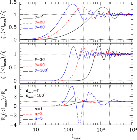
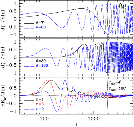
Figure 1: Left: A cumulative contribution of power spectra to $X$ from a limited range of $\ell<\ell_{\rm max}$ as a function of $\ell_{\rm max}$ (to be specific, the upper limit of the $\ell$-integration in equations (7) and (4) are truncated at $\ell_{\rm max}$), where $X$ stands for TPCF $\xi_{+}$ (top panel), $\xi_{-}$ (middle panel), or COSEBIs $E_{n}$ (bottom panel). All the results are normalized by their unlimited value. Here a combination of tomographic redshift bins of $z_{3}\times z_{3}$, and the WMAP9 cosmological model (Hinshaw et al., 2013) are adopted, but the results are insensitive to those choices. For TPCFs, three angular scales roughly corresponding to the minimum, intermediate, and maximum scales of H20 are shown. Vertical dotted lines show the $\ell$-range used in the Fourier space PS analysis by H19. Right: Integrands of the transformation between the power spectra to $\xi_{\pm}$ (top and middle panels, see equation (7)), or $E_{n}$ (bottom panel, see equation (4)). All integrands are normalized by their maximum value. The same angular scales shown in the left panels are shown except for $\xi_{\pm}$ where the intermediate case is omitted for clarity.

Right panels of Figure 1 compares differential contributions of power spectra to three two-point statistics ($\xi_{+}$, $\xi_{-}$, and $E_{n}$ from the top to bottom panels) as a function of $\ell$, to be specific, integrands of the relevant equations (equation (7) for $\xi_{\pm}$, and equation (4) for $E_{n}$). Left panels of Figure 1 compares cumulative contributions of power spectra to three two-point statistics ($\xi_{+}$, $\xi_{-}$, and $E_{n}$ from the top to bottom panels) from a limited range of $\ell<\ell_{\rm max}$ as a function of $\ell_{\rm max}$, to be specific, the upper limits of the $\ell$-integration in the relevant equations (equation (7) and (4)) are truncated at $\ell_{\rm max}$. For TPCFs, the three angular scales shown in the plots roughly correspond to the minimum, intermediate and maximum scales of H20. Vertical dotted lines show the $\ell$-range ($300<\ell<1900$) used in the Fourier space PS analysis by H19. One can see, from the figure, noticeable differences in $\ell$-ranges contributing to each three HSC-Y1 cosmic shear two-point statistics. Notably, $\xi_{+}$ has the broadest sensitivity range (non-zero ranges without the rapid oscillation in the differential contributions shown in the right panels of Figure 1), especially toward very low-$\ell$ modes. Compared to the TPCFs’ broad sensitivity range, our scale-cut of COSEBIs suppresses the sensitivity on both low- and high-$\ell$ modes, but a large part of contribution comes from modes with $\ell<300$. Therefore, we expect weak correlations in resulting cosmological parameter constraints between COSEBIs and TPCFs as well as between COSEBIs and PS, as in the case between PS and TPCFs found in H20, in which the two methods probe the different $\ell$-ranges and a 1$\sigma$ level difference in resulting $S_{8}$ constraints between PS and TPCFs was found (H20).

4 Measurements

4.1 Measurements of COSEBIs from the HSC-Y1 data

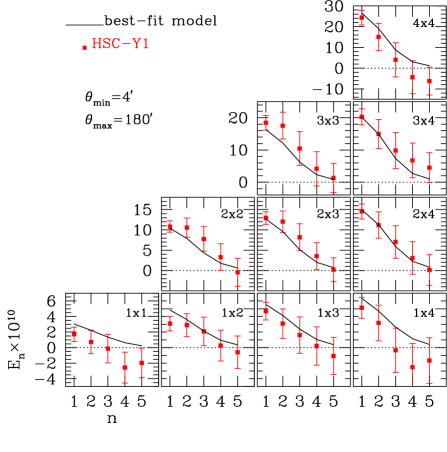
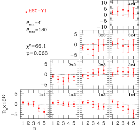
Figure 2: Comparison of the HSC-Y1 tomographic cosmic shear COSEBIs with the best-fitting theoretical model for the fiducial flat $\Lambda$CDM model. Top and bottom triangular-tiled panels show $E_{n}^{ab}$ and $B_{n}^{ab}$, respectively. Error bars represent the square-root of the diagonal elements of the covariance matrix. The solid lines in the top panels correspond to the best-fit (maximum likelihood) fiducial model.

The method of measuring COSEBIs precisely was developed and tested by Asgari et al. (2017, 2021). We confirmed the accuracy of the method adopted in Asgari et al. (2021) with HSC-Y1 mock catalogs (see Appendix A for details of this test), and we adopt it in this study. We first measure the cosmic shear TPCFs for two tomographic redshift bins $a$ and $b$ taking the shape weight into account as

$$\hat{\xi}_{\pm}^{ab}(\theta)={{\sum_{ij}w_{i}w_{j}\left[\hat{\gamma}_{i,t}^{a}(\vec{\theta}_{i})\hat{\gamma}_{j,t}^{b}(\vec{\theta}_{j})\pm\hat{\gamma}_{i,\times}^{a}(\vec{\theta}_{i})\hat{\gamma}_{j,\times}^{b}(\vec{\theta}_{j})\right]}\over{\sum_{ij}w_{i}w_{j}}},$$ (8)

where the tangential ($\hat{\gamma}_{t}$) and cross ($\hat{\gamma}_{\times}$) components of shear are defined with respect to the direction connecting a pair of galaxies under consideration ($i$ and $j$), $w_{i}$ is shape weight for each galaxy, and the summation runs over pairs of galaxies with their angular separation $\theta=|\vec{\theta}_{i}-\vec{\theta}_{j}|$ within an interval $\Delta\theta$ around $\theta$. Following Asgari et al. (2021), we adopt a fine $\log\theta$-binning, to be specific, 4000 bins over $0.5\arcmin<\theta<300\arcmin$ with an equal $\log\theta$-bin width, although we only use the limited range of $4\arcmin<\theta<180\arcmin$. For actual measurements of the TPCFs, we used the public software Athena (Schneider et al., 2002). We then perform the linear transformation in equations (2) and (3) to compute E/B-mode COSEBIs. We use the first five COSEBIs modes in the following analyses following the previous studies (Schneider et al., 2010; Asgari et al., 2012).

The measured signals are shown in Figure 2 with error bars representing the square-root of the diagonal elements of the covariance matrix (see Section 4.2). For comparison, the best-fit theoretical model obtained from the cosmological inference of our fiducial $\Lambda$CDM model (described in Section 6.1) is shown in the E-mode plots. The E-mode signals shown in Figure 2 form the data vector of our cosmological inference (see Section 5). We define the data vector as $d_{E,i}=(E_{1}^{11},E_{2}^{11},,,E_{5}^{11},E_{1}^{12},,,E_{5}^{44})$. Since there are 5 modes for each of 10 combinations of tomographic redshift bins, the data vector consists of 50 elements.

4.2 Covariance from HSC-Y1 mock catalogs

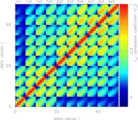
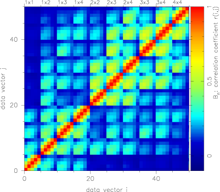
Figure 3: Covariance matrices normalized by the diagonal components, i.e., ${\rm Cov}_{ij}/\sqrt{{\rm Cov}_{ii}{\rm Cov}_{jj}}$, are shown. Top panel is for $E_{n}$, and bottom panel is for $B_{n}$. The x- and y-axis indicate elements of the data vector, which is defined as $d_{E,i}=(E_{1}^{11},E_{2}^{11},,,E_{5}^{11},E_{1}^{12},,,E_{5}^{44})$ and has 50 elements consisting of 10 tomographic combinations of COSEBIs (indicated as top label) each with 5 modes.

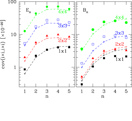
Figure 4: Diagonal components of covariance matrices of $E_{n}$ (left panel) and $B_{n}$ (right panel), to be specific $\langle X_{n}(z_{i}\times z_{j})X_{n}(z_{i}\times z_{j})\rangle$, are shown for four auto-correlation cases of tomographic redshift bins $z_{1}\times z_{1}$ (filled squares), $z_{2}\times z_{2}$ (filled triangles), $z_{3}\times z_{3}$ (open squares), and $z_{4}\times z_{4}$ (filled circles), from lowest to highest , respectively. Theoretical predictions (see text for details) are plotted with plus marks connected by dashed lines for visual help.

Following the methodology of the HSC-Y1 cosmic shear TPCF analysis by H20, we derive covariance matrices of the COSEBIs measurement using 2268 realizations of mock HSC-Y1 shape catalogs (see Shirasaki et al. (2019) for a detailed description of the mock catalogs). Since the HSC mock catalogs are constructed based on full-sky lensing simulation data with galaxy positions, intrinsic shape noise, and measurement noise taken from the real HSC-Y1 shape catalog, the mock data naturally have the same survey geometry and the same noise properties as the real catalog, and include super-survey cosmic shear signals from these full-sky lensing simulations. In addition, the effects of nonlinear structure formation on the lensing shear field are included in the mock data. Therefore the covariance matrix computed from the mock catalogs automatically includes all the contributions, namely, the shape noise, Gaussian, non-Gaussian, and super-survey covariance with the survey geometry being naturally taken into account.

We measure the cosmic shear COSEBIs for all 2268 mock catalogs in exactly the same manner as the real data measurement, and derive covariances for E- and B-mode COSEBIs. Results are shown in Figure 3, in which covariance matrices normalized by the diagonal components, i.e., ${\rm Cov}_{E,ij}/\sqrt{{\rm Cov}_{E,ii}{\rm Cov}_{E,jj}}$ are plotted. We show some diagonal components in Figure 4 so that the readers can grasp absolute values of the covariance matrices. In that figure, for rough comparison, approximate theoretical predictions of the covariance matrices are shown. To calculate them, we follow the prescription described in Appendix A of Asgari et al. (2020), and we take only major components into accounts; the Gaussian and shape noise terms for E-mode, and only the shape noise term for B-mode (see Barreira et al., 2018; Shirasaki et al., 2019, for contributions from non-Gaussian term and super sample covariance). Overall, reasonably good agreements between mock measurements and theoretical predictions can be seen in Figure 4. The disagreement between the mock covariance and the theoretical predictions presumably originates mainly from a simplified assumption to ignore the effect of survey geometry and masking in estimating the Gaussian and shape noise terms in the theoretical predictions (see Asgari et al., 2020). We note that these effects are properly taken into account in the mock covariance, which will be used in our cosmological analysis throughout the paper.

Shirasaki et al. (2019) studied in detail the accuracy on the estimation of the covariance matrix of cosmic shear TPCFs from the HSC-Y1 mocks, and investigated the impact of various systematic effects in the cosmic shear analysis, including photo-$z$ errors and the uncertainty in the multiplicative bias, on the covariance estimation. Based on their results, H20 concluded that the covariance matrix of TPCFs estimated from the mocks is calibrated with $<10\%$ accuracy against various systematic effects in the cosmic shear analysis (see section 4.4 of H20). Since the COSEBIs are linearly related to TPCFs, a similar level of accuracy can be expected for the covariance matrix of COSEBIs measurement. It should be noted that the cosmology dependence of the covariance cannot be included in our mock based approach, because the HSC-Y1 mock catalogs are based on a set of full-sky gravitational lensing ray-tracing simulations that adopt a specific flat $\Lambda$CDM cosmology (Takahashi et al., 2017). In the HSC-Y1 cosmic shear PS analysis by H19, the effect of the cosmology dependence of the covariance on their cosmological inference was examined by comparing cosmological constraints derived using the cosmology-dependent covariance (which is their fiducial model) with those derived using a cosmology-independent one (fixed to the best-fit cosmological model). They found that the best-fit $\Omega_{m}$ and $S_{8}(=\sigma_{8}(\Omega_{m}/0.3)^{\alpha}$ with $\alpha=0.45$ or $0.5$) values agree with each other within 20% of the statistical uncertainty. Based on this result, we assume that the cosmology dependence of the covariance matrix does not significantly impact our cosmological analysis.

Using the mock $E_{n}^{ab}$ data vectors and their covariance matrix obtained above, we examine the Gaussianity of the likelihood function of cosmic shear COSEBIs as it is a basic assumption in the standard Bayesian likelihood analysis. Specifically, we check a necessary condition of the Gaussianity; whether a distribution of $\chi^{2}$ measured from 2268 mock samples follows the theoretical $\chi^{2}$ distribution with the same degrees-of-freedom. We compute, for each mock data, the standard $\chi^{2}$,

$$\chi_{E}^{2}=\sum_{i,j}(d_{E,i}-\bar{d}_{E,i}){\rm Cov}_{E,ij}^{-1}(d_{E,j}-\bar{d}_{E,i}),$$ (9)

where $d_{E,i}$ is the E-mode data vector consisting of 10 tomographic combinations of $E_{n}^{ab}$ each with 5 modes and thus having 50 elements, $\bar{d}_{E,i}$ is its average among 2268 mock samples, and ${\rm Cov}_{E,ij}$ is the E-mode covariance matrix. We perform a Kolmogorov–Smirnov (KS) test for the distribution of mock $\chi_{E}^{2}$ against the theoretical $\chi^{2}$ distribution, and obtain the KS $p$-value of 0.11. Thus we conclude that the mock $\chi_{E}^{2}$ distribution is in a reasonable agreement with the theoretical one.

4.3 B-mode null test

Here, we quantitatively test the consistency of the B-mode COSEBIs signals with zero using the standard $\chi^{2}$ statistics,

$$\chi_{B}^{2}=\sum_{i,j}d_{B,i}{\rm Cov}_{B,ij}^{-1}d_{B,j},$$ (10)

where $d_{B,i}$ is the B-mode data vector (presented in Figure 2), and ${\rm Cov}_{B,ij}$ is the B-mode covariance matrix presented in Figure 4. We find $\chi_{B}^{2}=66.1$ for 50 degrees-of-freedom, corresponding to the $p$-value of 0.063. Therefore we conclude that no evidence for a significant B-mode signal is found.

We also compute the B-mode $\chi_{B}^{2}$ for each of 2268 mock catalogs. We compare the distribution of them with the theoretical $\chi^{2}$ distribution, and find a good agreement between them. We find that 135 cases out of 2268 mock samples exceed the observed B-mode $\chi_{B}^{2}$ values of 66.1, corresponding to a probability of 0.060 which is in a good agreement with the $p$-value estimated above.

5 Cosmological analyses

We employ the standard Bayesian likelihood analysis for the cosmological inference of measured E-mode COSEBIs. The log-likelihood is given by

$$-2\ln{\cal L}(\bm{p})=\sum_{i,j}\left(d_{i}-m_{i}(\bm{p})\right){\mbox{Cov}}_{ij}^{-1}\left(d_{j}-m_{j}(\bm{p})\right),$$ (11)

where $d_{i}$ is the E-mode data vector consisting of 10 tomographic combinations of $E_{n}^{ab}$ each with 5 modes presented in Section 4.1, $m_{i}(\bm{p})$ is the theoretical model with $\bm{p}$ being a set of parameters detailed in Section 5.1, and ${\mbox{Cov}}_{ij}$ is the covariance matrix presented in Section 4.2. Since our covariance matrix is constructed from 2268 mock realizations, its inverse covariance is known to be biased high (see Anderson, 2003; Hartlap et al., 2007, and references therein). When calculating the inverse covariance, we therefore include the so-called Anderson-Hartlap correction factor $\alpha=(N_{\mbox{mock}}-N_{d}-2)/(N_{\mbox{mock}}-1)$, where $N_{\mbox{mock}}=2268$ is the number of mock realizations and $N_{d}=50$ is the length of our data vector.

In order to sample the likelihood efficiently, we employ the multimodal nested sampling algorithm (Feroz & Hobson, 2008; Feroz et al., 2009, 2019), as implemented in the public software MultiNest.

5.1 Model parameters

In this subsection, we summarize model parameters and their prior ranges used in our cosmological analysis. Prior ranges and choice of parameter set for systematic tests are summarized in Table 5.1.

Summary of cosmological, astrophysical, and systematics parameters used in our cosmological analysis. “flat[$x_{1}$, $x_{2}$]” means a flat prior between $x_{1}$ and $x_{2}$, whereas “Gauss($\bar{x}$, $\sigma$)” means a Gaussian prior with the mean $\bar{x}$ and the standard deviation $\sigma$. For detail descriptions of parameters, see section 5.1.1 for the cosmological parameters, section 5.1.2 for the astrophysical nuisance parameters, and section 5.1.3 for the systematics nuisance parameters. Parameter                         Prior range Section Fiducial $\Lambda$CDM $w$CDM Systematics tests Cosmological 5.1.1 $\Omega_{c}$ flat[0.01, 0.9] $\sigma_{8}$ flat[0.1, 2] $\Omega_{b}$ flat[0.038, 0.053] $n_{s}$ flat[0.87, 1.07] $h$ flat[0.64, 0.82] $\sum m_{\nu}$ [eV] fixed to 0.06 flat[0, 0.5] for “$\sum m_{\nu}$ varied“ $w$ fixed to -1 flat[$-2$, $-1/3$] Astrophysical 5.1.2 $A_{\mbox{IA}}$ flat[-5, 5] fixed to 0 for “w/o IA” $\eta_{\mbox{IA}}$ flat[-5, 5] fixed to 3 for “IA $\eta_{\mbox{IA}}=3$” $A_{B}$ fixed to 0 fixed to 1 for “$A_{B}=1$” or flat[-5, 5] for “$A_{B}$ varied” Systematics 5.1.3 $A_{\mbox{psf}}$ Gauss(1, 1) fixed to 0 for “w/o PSF error” Appendix B.1 $\Delta m$ Gauss(0, 0.01) fixed to 0 for “w/o $\Delta m$” $\Delta z_{1}$ Gauss(0, 0.0374) fixed to 0 for “w/o $p(z)$ error” $\Delta z_{2}$ Gauss(0, 0.0124) fixed to 0 for “w/o $p(z)$ error” $\Delta z_{3}$ Gauss(0, 0.0326) fixed to 0 for “w/o $p(z)$ error” $\Delta z_{4}$ Gauss(0, 0.0343) fixed to 0 for “w/o $p(z)$ error” $A_{\langle\gamma\rangle}$ fixed to 0 flat[-5, 5] for “w/ const-$\gamma$” Appendix B.2

5.1.1 Cosmological parameters

We focus on the flat $\Lambda$CDM cosmological model characterized by five parameters; the density parameter of CDM ($\Omega_{c}$), the normalization of matter fluctuation ($\sigma_{8}$), the density parameter of baryons ($\Omega_{b}$), the Hubble parameter ($h$), and the scalar spectrum index ($n_{s}$). Among those parameters, the cosmic shear COSEBIs are most sensitive to $\Omega_{c}$ and $\sigma_{8}$. Thus we adopt prior ranges that are sufficiently wide for these parameters (see Table 5.1). Note that in contrast to H20 in which $A_{s}$ (the scalar amplitude of the linear matter power spectrum on $k=0.05$ Mpc^-1) was adopted for the amplitude parameter of the linear CDM power spectrum, we adopt $\sigma_{8}$ because for the cosmic shear or more generally low-redshift probes of large-scale structure, observables are more directly sensitive to $\sigma_{8}$. We treat $A_{s}$ as a derived parameter. For $\Omega_{b}$, $n_{s}$, and $h$, which are only weakly constrained with cosmic shear COSEBIs, we set prior ranges which largely bracket allowed values from external experiments (see Table 5.1). For the sum of neutrino mass, we take $\sum m_{\nu}=0.06$ eV from the lower bound indicated by the neutrino oscillation experiments (e.g., Lesgourgues et al., 2013, for a review) for our fiducial choice. As a systematics test, we check the impact of neutrino mass on our conclusions by varying $\sum m_{\nu}$.

In addition to the fiducial $\Lambda$CDM model, we consider an extended model by including the time-independent equation-of-state parameter for the dark energy ($w$), referred to as the $w$CDM model. We take a flat prior with $-2<w<-1/3$, which excludes the non-accelerating expansion of the present day Universe, and brackets allowed values from external experiments.

5.1.2 Astrophysical parameters

In theoretical modeling of the COSEBIs signal, we include two astrophysical effects; one is the effect of baryon physics on the nonlinear matter power spectrum (see Section 3.2), and the other is the contribution of the intrinsic alignment (IA) of galaxy shapes (see Kirk et al., 2015; Troxel & Ishak, 2015, for recent reviews). Below we summarize our treatment of those effects in our cosmological analyses.

In modeling baryonic effect, we follow the methodology of Köhlinger et al. (2017), in which a modification of the dark matter power spectrum due to the AGN feedback is modeled by the fitting function derived by Harnois-Déraps et al. (2015), but an additional parameter ($A_{B}$) that controls the strength of the feedback is introduced (see Section 5.1.2 of Köhlinger et al., 2017, for the explicit expression). We note that H19 and H20 employed the same methodology. However, since we impose the scale-cut of cosmic shear COSEBIs conservatively so that the baryon effects do not have a significant impact on our analysis (see Section 3.3), we do not include the baryon effect in our fiducial model, but check its impact in our systematics tests; one fixing $A_{B}=1$ that corresponds to the original AGN feedback model, and the other in which $A_{B}$ is a free parameter (see Table 5.1).

The IA comes both from the correlation between intrinsic shapes of two physically associated galaxies in the same local field (referred to as the II-term) and from the cross correlation between lensing shear of background galaxies and the intrinsic shape of foreground galaxies (referred to as the GI-term). We employ the standard theoretical framework for these terms, namely, the nonlinear modification of the tidal alignment model (Hirata & Seljak, 2004; Bridle & King, 2007; Joachimi et al., 2011). In this model, the E-mode COSEBIs originating from II and GI terms are given in a similar manner as the cosmic shear COSEBIs, equation (4), but with IA power spectra $P_{\mbox{II}}^{ab}(\ell)$ and $P_{\mbox{GI}}^{ab}(\ell)$ (see equations (12) and (13) of H20 for explicit expressions for those terms). Following H20, we adopt the standard parametric IA model with two parameters, the amplitude parameter $A_{\mbox{IA}}$ and the power-law redshift dependence parameter $\eta_{\mbox{IA}}$ that represents the effective redshift evolution of the IA amplitude. Following recent cosmic shear studies e.g., Hildebrandt et al. (2017), Troxel et al. (2018), and H19, we adopt wide prior ranges for these parameters (see Table 5.1).

5.1.3 Systematic parameters

Our treatment of systematic effects in the cosmological analysis largely follows that in H20. To summarize, in our fiducial model we take account of systematic effects from PSF leakage and PSF modeling errors, the uncertainty in the shear multiplicative bias correction, and uncertainties in the source galaxy redshift distributions. In addition, in systematics tests we check the impact of the uncertainty of the constant shear over fields. Below we summarize our modeling of those systematic effects, and choices for prior ranges on nuisance parameters in these models.

Our models for the PSF leakage and PSF modeling errors are described in Appendix B.1. We apply the correction for these systematics by equation (20), which has one nuisance parameter $A_{\rm psf}$. We adopt a Gaussian prior with $({\rm mean},\sigma)=(1,1)$ for it and include them in our fiducial model.

Regarding the uncertainty in the shear multiplicative bias correction, we follow H20 (see Section 5.2.3 of H20). In short, we introduce the nuisance parameter $\Delta m$, which represents the residual multiplicative bias, and modifies the theoretical prediction for the COSEBIs to

$$E_{n}^{ab}\rightarrow(1+\Delta m)^{2}E_{n}^{ab}.$$ (12)

A Gaussian prior with $({\rm mean},\sigma)=(0,0.01)$ is taken for $\Delta m$ based on the calibration of the HSC-Y1 shear catalog (Mandelbaum et al., 2018b).

Regarding uncertainties in the redshift distributions of source galaxies, we again follow H20. Introducing a nuisance parameter $\Delta z_{a}$ for each tomographic redshift bin, the source redshift distribution, $p^{a}(z)$, is shifted by $p^{a}(z)\rightarrow p^{a}(z+\Delta z_{a})$. Gaussian priors are taken for $\Delta z_{a}$ with the same mean and $\sigma$ as those adopted in H20 (see Table 5.1).

Finally, as described in Appendix B.2, we model a contribution to E-mode COSEBIs arising from a constant shear by equation (22), which has one nuisance parameter $A_{\langle\gamma\rangle}$. We assume a redshift-independent constant shear for simplicity. Given that we have not found a strong evidence of the existence of the residual constant shear (see Appendix 1 of H20), we do not include it in our fiducial model, but check its impact as a systematics test, in which we take a flat prior of $-5<A_{\langle\gamma\rangle}<5$.

6 Results

We first present cosmological constraints from our cosmic shear COSEBIs analysis in the fiducial flat $\Lambda$CDM model. We then discuss the robustness of the results against various systematics, and present results from internal consistency checks among different choices of tomographic redshift bins and scale-cuts. We compare our cosmological constraints with other cosmic shear results and Planck CMB result. We also compare our results with those from the HSC-Y1 cosmic shear PS and TPCF analyses, and examine the consistency among them using mock HSC-Y1 catalogs.

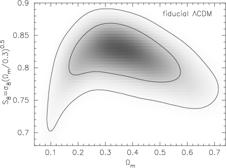
Figure 5: Marginalized posterior contours (68% and 95% confidence levels) with the gray scale for a visual overview of the distribution (darker for higher posterior) in the $\Omega_{m}$-$\sigma_{8}$ plane (top panel) and in the $\Omega_{m}$-$S_{8}$ plane (bottom panel), where $S_{8}=\sigma_{8}\sqrt{\Omega_{m}/0.3}$, in the fiducial flat $\Lambda$CDM model. In the $\Omega_{m}$-$\sigma_{8}$ panel, three constant $S_{8}$ loci ($S_{8}=0.7$, 0.8 and 0.9 from bottom to top, respectively) are shown by dashed blue curves.

Figure 6: The upper three rows show the marginalized one-dimensional posterior distributions of model parameters in the fiducial flat $\Lambda$CDM model; the cosmological parameters are in the top-row, and the astrophysical and systematics parameters are in two middle rows. Three panels in the bottom-row are for derived parameters. For parameters with flat prior ranges, the plotted range of the horizontal-axis indicates its prior range. For parameters with Gaussian priors, Gaussian priors are shown by the dashed curves. Dotted vertical lines represent the approximate 68% credible intervals, which are not shown for poorly constrained parameters.

6.1 Cosmological constraints in the fiducial flat $\Lambda$CDM model

Means and 68% confidence intervals of marginalized posterior distributions for well constraint cosmological parameters. Parameter Mean 68% confidence interval $\Omega_{c}$ 0.319 0.169 - 0.447 $\Omega_{m}$ 0.365 0.218 - 0.492 $A_{s}\times 10^{9}$ 1.46 0.411 - 2.50 $\sigma_{8}$ 0.780 0.576 - 0.883 $S_{8}$ 0.809 0.783 - 0.844

First, we present results for our fiducial flat $\Lambda$CDM model. Marginalized posterior contours in the $\Omega_{m}$-$\sigma_{8}$ and $\Omega_{m}$-$S_{8}$ planes are shown in Figure 5, and marginalized one-dimensional posterior distributions of 13 model parameters and 3 derived parameters are shown in Figure 6. We find marginalized 68% confidence intervals of $0.218<\Omega_{m}<0.492$, $0.576<\sigma_{8}<0.883$, and $0.783<S_{8}<0.844$ (see also Table 6.1).

From the posterior distributions shown in Figure 6, it can be seen that the HSC-Y1 cosmic shear COSEBIs alone cannot place useful constraints on 3 out of 5 input cosmological parameters ($\Omega_{b}$, $n_{s}$ and $H_{0}$), but we confirm that the constraint on $S_{8}$ is not strongly affected by uncertainties in these parameters as long as they are restricted within the prior ranges considered in this study.

It is also found from two middle rows of Figure 6 that except for $A_{\mbox{IA}}$, one-dimensional posteriors of astrophysical and systematics parameters are dominated by priors. In the following subsections, we discuss effects of these nuisance parameters on the cosmological inference by changing the parameter setup.

In Figure 2, we compare the measured cosmic shear COSEBIs signals with the theoretical model with best-fit parameter values for the fiducial flat $\Lambda$CDM model. In these plots, error bars represent the square-root of the diagonal elements of the covariance matrix. We find that our model with the fiducial parameter setup reproduces the observed signals quite well. The $\chi^{2}$ value for the best-fit parameter set is $\chi^{2}=40.7$ for the effective degree-of-freedom of $50-3=47$, resulting in a $p$-value of 0.73.

6.2 Systematics tests

Figure 7: Means and 68% credible intervals of marginalized one-dimensional constraints on $S_{8}=\sigma_{8}\sqrt{\Omega_{m}/0.3}$. The fiducial case (top) is compared with different setups to check the robustness of our result. Vertical dotted lines show the 68% credible interval of the fiducial case. See Figure 17, for comparisons of constraints in the $\Omega_{m}$-$\sigma_{8}$ plane.

In our cosmological analysis, we have a number of astrophysical and systematics nuisance parameters that are marginalized over. Also, we have four model parameters that are fixed to the fiducial values in our fiducial setup (namely, $\sum m_{\nu}$, $w$, $A_{B}$, and $A_{\langle\gamma\rangle}$, see Table 5.1), but may have, in principle, an impact on the cosmological inference. Below, we discuss effects of these nuisance parameters on the cosmological inference by changing the parameter setup (see Table 5.1 for parameter setups, and following subsections for details). In addition, we also perform an empirical test on robustness of our cosmological constraints against possible uncertainties in the source redshift distributions by replacing the default ones derived from the COSMOS re-weighted method with ones derived from stacked PDFs with three photo-$z$ methods, DEmP, Ephor AB, and FRANKEN-Z (see subsection 6.2.7, and Section 2.2 of H20 for details).

We focus on $S_{8}$ constraints to assess the impact of the nuisance parameters and source redshift distributions as it is a primary parameter to be constrained by cosmic shear two-point statistics. The results of these systematics tests are summarized in Figure 7, in which credible intervals of marginalized one-dimensional posterior distributions of $S_{8}$ derived from systematics tests are compared with that of the fiducial setup. In this comparison, we use $S_{8}=\sigma_{8}(\Omega_{m}/0.3)^{\alpha}$ with $\alpha=0.5$. In Appendix C, we also present comparisons of marginalized posterior contours in the $\Omega_{m}$-$\sigma_{8}$ plane because a single choice of $\alpha$ does not always provide an optimal description for the $\sigma_{8}$-$\Omega_{m}$ degeneracy, especially for cases with broad confidence contours such as ours. Overall, we find that no significant impact on our $S_{8}$ constraint is found from the systematics tests, as described in detail in following subsections.

6.2.1 Intrinsic galaxy alignment

We find that the marginalized one-dimensional constraint on $A_{\mbox{IA}}$ obtained from our fiducial cosmological inference is $A_{\mbox{IA}}=0.44_{-0.31}^{+0.46}$ , which is consistent with the results from the HSC-Y1 TPCF ($A_{\mbox{IA}}=0.91_{-0.32}^{+0.27}$, H20) and PS analyses ($A_{\mbox{IA}}=0.38\pm 0.70$, H19) for their fiducial setup.

In order to test the robustness of the cosmological constraints against the uncertainty of the intrinsic galaxy alignment, we perform two cosmological inferences with different IA modeling. In one case, the IA contribution is completely ignored i.e., $A_{\mbox{IA}}$ is fixed to 0 (“w/o IA” setup), and in the other case $\eta_{\mbox{IA}}$ is fixed to 3 while $A_{\mbox{IA}}$ is treated as a free parameter (“IA $\eta_{\rm IA}=3$” setup, see section 5.4 of H19 for the reasoning of this choice). The results from these settings are compared with the fiducial one in Figure 7 (see panels (a) and (b) of Figure 17 for constraints in $\sigma_{8}$-$\Omega_{m}$ plane). We find that in both of the two cases, the changes in cosmological constraints are not significant. On those grounds, we conclude that the effects of uncertainty in IA modeling on our fiducial cosmological constraints is insignificant.

6.2.2 Baryonic feedback

Figure 8: Marginalized one-dimensional posterior distributions of nuisance parameters derived from non-fiducial models. Top-left panel is for the baryon feedback model parameter from the “$A_{B}$ varied” setup, top-right panel is for the neutrino mass from the “$\sum m_{\nu}$ varied” setup, and the bottom panel is for the residual constant shear $A_{\langle\gamma\rangle}$ from the “w/const-$\gamma$” setup.

In our fiducial setup, we do not include the effect of the baryonic feedback, but instead we impose the conservative scale-cut so that the baryon effects do not have a significant impact on our analysis (see Section 3.3). It is therefore expected that the baryonic feedback effect does not strongly affect our cosmological constraints. We check this explicitly by employing an empirical model described in Section 5.1.2 (see Section 4.1.1 of H20 for details). Following H20, we consider two cases; the original AGN feedback model by Harnois-Déraps et al. (2015), which corresponds to fixing the baryon feedback parameter $A_{B}=1$ (“$A_{B}=1$” setup), and a more flexible model in which $A_{B}$ is allowed to vary with a flat prior in the range $-5<A_{B}<5$ (“$A_{B}$ varied” setup). From the results shown in Figure 7 (and see panels (c) and (d) of Figure 17 for constraints in $\sigma_{8}$-$\Omega_{m}$ plane), we find that in both of the two cases, the changes in cosmological constraints are not significant. The marginalized one-dimensional posterior distribution of $A_{B}$ obtained from the “$A_{B}$ varied” setup is shown in Figure 8, from which it is found that the constraint on $A_{B}$ is very weak with $A_{B}=2.0\pm 1.2$ (mean and $\sigma$). We also find that the correlation between $A_{B}$ and $S_{8}$ is very week. Based on these results, we conclude that the effect of baryonic feedback on our fiducial cosmological constraints is insignificant.

6.2.3 Neutrino mass

In our fiducial setup, the neutrino mass is fixed at $\sum m_{\nu}=0.06$ eV. Since the non-zero neutrino mass leads to a redshift-dependent suppression of the matter power spectrum on small scales, it has, in principle, an impact on our cosmological inference. However, the HSC-Y1 cosmic shear analyses are expected to be insufficient to place a useful constraint on the neutrino mass due to the current measurement precision and the scale-cuts on small scales, and this is indeed the cases for HSC-Y1 PS (H19) and TPCF analyses (H20). We find that this is also the case for our COSEBIs analysis; Figure 8 shows the one-dimensional posterior distribution of $\sum m_{\nu}$ obtained from the “$\sum m_{\nu}$ varied” setup in which the neutrino mass is allowed to vary with a flat prior in the range $0<\sum m_{\nu}<0.5$ eV. The credible interval on $S_{8}$ is compared with the fiducial case in Figure 7 (see panel (e) of Figure 17 for $\sigma_{8}$-$\Omega_{m}$ constraints). It is found from this comparison result that the non-zero neutrino mass indeed has little impact on our cosmological constraints.

6.2.4 Residual constant shear

Here we check the robustness of our fiducial cosmological constraints against the residual constant shear that is not included in our fiducial model. To do so, we test the same setup as in the fiducial case but including a contribution from residual constant shear by equation (22) with a nuisance parameter $A_{\langle\gamma\rangle}$ that controls its amplitude (“w/ const-$\gamma$” setup, see Appendix B.2 for details). We adopt a flat prior in the range $-5<A_{\langle\gamma\rangle}<5$. The derived $S_{8}$ constraint is compared with the fiducial case in Figure 7 (see also panel (f) of Figure 17). We find that the resulting changes in the cosmological constraints are very small. The marginalized one-dimensional posterior distribution of $A_{\langle\gamma\rangle}$ is shown in Fig 8, and its mean and $\sigma$ are found to be $A_{\langle\gamma\rangle}=0.0\pm 1.1$, which is consistent with the constant shear expected from the cosmic shear that is coherent over the field (see Appendix 1 of H20).

6.2.5 PSF leakage and PSF modeling errors

Following the previous HSC-Y1 cosmic shear analyses (H19 and H20), we employ the conventional model for the PSF leakage and PSF modeling errors given by equation (14). We then derive an empirical model for a contribution to the measured E-mode COSEBIs by equation (20) with a nuisance parameter $A_{\rm psf}$ that controls its amplitude (see Appendix B.1 for details), for which we adopt a Gaussian prior of $({\rm mean},\sigma)=(1,1)$. Marginalized one-dimensional posterior distributions of these parameters from our fiducial analysis are shown in Figure 6. We find that the posterior is largely determined by the prior. We also find that the marginalized constraint on $A_{\rm psf}$ is not strongly correlated with either $\Omega_{m}$, $\sigma_{8}$, or $S_{8}$.

In order to check the robustness of our cosmological constraints against these systematics, we test the same setup as the fiducial case but ignoring them i.e., setting $A_{\rm psf}=0$ (“w/o PSF error” setup). The result is shown in Figure 7 (see also panel (g) of Figure 17). We find that the changes in the cosmological constraints are very small as a natural consequence of PSF leakage and PSF modeling errors being smaller than the size of errors on the HSC-Y1 cosmic shear COSEBIs.

6.2.6 Shear calibration error

In our fiducial analysis we also take account of the uncertainty in the shear multiplicative bias correction using a simple model, equation (12), with a Gaussian prior corresponding to a 1% uncertainty (see Section 5.1.3). The marginalized one-dimensional posterior distribution of the model parameter $\Delta m$ from our fiducial analysis is shown in Figure 6, which indicates that the posterior is dominated by the prior.

In order to check the effect of this residual calibration bias on our cosmological constraints, we test the same setup as the fiducial case but ignoring the nuisance parameter i.e., setting $\Delta m=0$ (“w/o $\Delta m$” setup). The result is shown in Figure 7 (see also panel (h) of Figure 17). We find that the changes in the cosmological constraints are very small.

6.2.7 Source redshift distribution errors

In our fiducial analysis, we introduce nuisance parameters $\Delta z_{a}$, which represent a shift of each of the source redshift distributions To be specific, the source redshift distribution, $p^{a}(z)$, is shifted by $p^{a}(z)\rightarrow p^{a}(z+\Delta z_{a})$ (see Section 5.1.3). Marginalized one-dimensional posterior distributions of these parameters from our fiducial analysis are shown in Figure 6. Although peak positions of these posteriors show shifts from the peak the prior distributions, the sizes of the shifts are within 1$\sigma$ of the Gaussian priors, and thus are not statistically significant. We note that a relatively large shift seen for the lowest redshift bin is also seen in HSC-Y1 TPCF analysis with a similar size and direction (H20), and thus it may indicate an unknown bias in estimation of the source redshift distribution that is not captured in the prior knowledge.

In order to check the robustness of our cosmological constraints against these uncertainties, we test the same setup as the fiducial analysis but ignoring these parameters (“w/o $p(z)$ error” setup). The result is shown in Figure 7 (see also panel (i) of Figure 17). We find that the changes in the cosmological constraints are very small.

In addition, following H20, we also perform an empirical test; we replace the default source redshift distributions derived from the COSMOS re-weighted method with ones derived from stacked PDFs with three photo-$z$ methods, DEmP, Ephor AB, and FRANKEN-Z (see Section 2.2 of H20 for details). Other settings remain the same as the fiducial setup. The results are shown in Figure 7 (labeled as “$P(z)$ method”, see also panels (j), (k), and (l) of Figure 17). Again, we find that the changes in the cosmological constraints are not significant, and thus we conclude that no additional systematics are identified from this test.

6.3 Internal consistency

Figure 9: Means and 68% credible intervals of marginalized one-dimensional constraints on $S_{8}$. The “cosmology alone” case (top) is compared with different setups for internal consistency checks. Vertical dotted lines show the 68% credible interval of the cosmology alone case. See Figure 18, for comparisons of constraints in the $\Omega_{m}$-$\sigma_{8}$ plane.

Here we present results of internal consistency checks in which we derive cosmological constraints from subsets of the data vector, and from data vectors generated with smaller-/larger-half scale-cuts than the original scale-cut range, and then we compare derived cosmological constraints with the ones from a reference setup. In doing so, following H20, we do not use the fiducial results as the reference, but instead we adopt the results from the “cosmology alone” setup in which we include neither systematics nor astrophysical parameters but only five cosmological parameters are included as a baseline for comparison. The reason for this choice is to avoid undesirable changes in nuisance parameters, which may add or cancel out shifts in parameter constraints. Of course, for this test to be meaningful, the reference setup must provide cosmological constraints that are consistent with ones from fiducial case, which we explicitly confirmed.

6.3.1 Tomographic redshift bins

First, we exclude one of the four redshift bins, and perform the cosmological inference with the remaining three tomographic bins. The resulting marginalized constraints on $S_{8}$ are shown in Figure 9 (see also panels of (a) to (d) of Figure 18 for marginalized constraints in $\Omega_{m}$-$\sigma_{8}$ plane). We find that constraints on $S_{8}$ from test setups are consistent within 1$\sigma$ of the reference result. Also it is seen in Figure 18 that 68% credible contours in the $\Omega_{m}$-$\sigma_{8}$ plane in these cases largely overlap with the reference contour. Thus we conclude that no significant internal inconsistency is found from this test.

6.3.2 Different scale-cuts

Next, we check the internal consistency among different angular ranges by splitting the original scale-cut ($4\arcmin<\theta<180\arcmin$) into two scale-cuts ($4\arcmin<\theta<27\arcmin$ and $27\arcmin<\theta<180\arcmin$). We generate the data vectors and covariance matrices for these two scale-cuts following the same procedure as for the fiducial scale-cut. The resulting marginalized constraints on $S_{8}$ are shown in Figure 9. As expected, the credible intervals are larger than the reference case. We see that the smaller-half scale-cut has more constraining power than the larger-half scale-cut. In addition, some more information on this can be seen in the comparison plots in the $\Omega_{m}$-$\sigma_{8}$ plane (panels of (e) and (f) of Figure 18): The smaller-half scale-cut places constraint contours which are as tight as the reference contours in the $S_{8}$ direction (perpendicular to the $\Omega_{m}$-$\sigma_{8}$ degeneracy direction), but are very elongated in the degeneracy direction. Thus from these results we see that a wider angular range is effective in placing a tighter constraint in $\Omega_{m}$-$\sigma_{8}$ plane. Overall, the results from the larger/smaller-half scale-cuts are consistent with the reference results. Thus we again conclude that no significant internal inconsistency is found from this test.

6.4 $w$CDM model

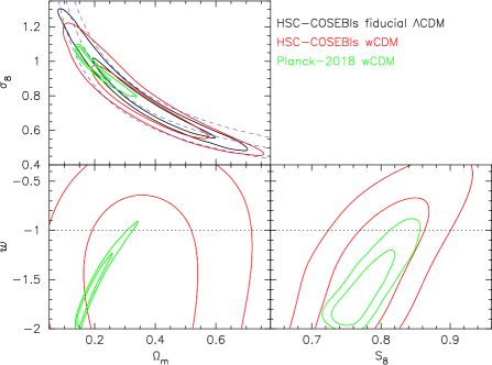
Figure 10: Marginalized posterior contours (68% and 95% confidence levels) in the $\Omega_{m}$-$\sigma_{8}$ plane (top), the $\Omega_{m}$-$w$ plane (bottom left) and the $S_{8}$-$w$ plane (bottom right) in the $w$CDM model are shown by red contours. Constraints from the fiducial $\Lambda$CDM model are shown by black contours, and Planck 2018 results for the $w$CDM model (Planck Collaboration et al., 2020a, TT+TE+EE+lowE) are also shown by green contours. In the $\Omega_{m}$-$\sigma_{8}$ panel, three constant $S_{8}$ loci ($S_{8}=0.7$, 0.8 and 0.9 from bottom to top, respectively) are shown by dashed blue curves.

In addition to the fiducial $\Lambda$CDM model, we test one extended model by including the time-independent dark energy equation of state parameter $w$, although it was found in H19 and H20 that HSC-Y1 cosmic shear two-point statistics alone cannot place a useful constraint on $w$. We allow $w$ to vary with a flat prior in the range $-2<w<-1/3$. The setup of the other parameters are the same as the fiducial $\Lambda$CDM model.

The marginalized constraints in the $\Omega_{m}$-$\sigma_{8}$, $\Omega_{m}$-$w$, and $S_{8}$-$w$ planes are shown in Figure 10, along with constraints from the fiducial $\Lambda$CDM model and the Planck 2018 results for the $w$CDM model (Planck Collaboration et al., 2020a, TT+TE+EE+lowE). As can be seen from the Figure, our constraints on those parameters are consistent with the Planck’s results, although Planck’s constraints are much tighter than our constraints. Marginalized one-dimensional constraint range of $S_{8}$ is shown in Figure 7. It is found that the derived two-dimensional marginalized posterior distributions are similar to those obtained from the HSC-Y1 cosmic shear TPCF (see figure 14 of H20) and PS (see figure 16 of H19) analyses, as expected.

6.5 Comparison to other constraints from the literature

Figure 11: 68% credible intervals of marginalized posterior distributions of $S_{8}=\sigma_{8}\sqrt{\Omega_{m}/0.3}$ or that of the projected joint highest posterior density (PJ-HPD) for KiDS-1000. Our result from the fiducial $\Lambda$CDM model is compared with other results in the literature, HSC first year (HSC-Y1) cosmic shear TPCF (H20), PS (H19), DES-Y3 cosmic shear TPCFs (their fiducial and $\Lambda$CDM-Optimized models are shown, see Amon et al., 2022, for details), KiDS-1000 cosmic shear COSEBIs (Asgari et al., 2021), and Planck 2018 CMB (Planck Collaboration et al., 2020a, TT+TE+EE+lowE). Since different studies adopt different definitions of the central values (mean, median or peak of the marginalized posterior distribution, or the multivariate maximum posterior), central values are not shown to avoid possible misunderstanding. Note that since different studies adopt different priors and modeling, part of the differences in the credible intervals may be due to the different choices of priors and modeling. See Figure 19 for comparisons of constraints from those studies in the $\Omega_{m}$-$\sigma_{8}$ plane.

Next, we compare the cosmological constraints from our fiducial $\Lambda$CDM model with results from other cosmic shear and CMB measurements. Figure 11 compares the 68% credible intervals of $S_{8}=\sigma_{8}\sqrt{\Omega_{m}/0.3}$, where results of other projects are taken from the literature. See also Figure 19 for comparison to other results in $\Omega_{m}$-$\sigma_{8}$ plane.

DES-Y3 (Amon et al., 2022) covers a much larger area (4143 deg²) than the HSC-Y1, yielding tighter constraints than our fiducial results. Note that in their cosmological analyses, the neutrino mass density is allowed to vary. They provide results from two models; their fiducial model adopts a very conservative small-scale cut yielding a broader constraint than the one from their $\Lambda$CDM-Optimized model in which smaller scale information are used safely (see Amon et al., 2022). In both cases, their $S_{8}$ constraints are lower than ours, and their $\Lambda$CDM-Optimized model is in about 1.0$\sigma$ difference from our fiducial result (see Figure 11).

KiDS-1000 covers an effective area of 777.4 deg² (Asgari et al., 2021). They employed three two-points statistics; the TPCF, band power spectra, and COSEBIs, and found cosmological results from these three to be in excellent agreement. Their $S_{8}$ value from COSEBIs analysis is lower than ours and is in about 1.4$\sigma$ difference from our fiducial result (see Figure 11).

The credible interval of $S_{8}$ from Planck 2018 (Planck Collaboration et al., 2020a, we take TT+TE+EE+lowE without CMB lensing) is consistent with our result. It is also found from Figure 19 that the credible contours in the $\Omega_{m}$-$\sigma_{8}$ plane from the Planck 2018 CMB result overlap well with our result. We therefore conclude that there is no tension between Planck 2018 constraints and HSC-Y1 cosmic shear COSEBIs constraints as far as $S_{8}$, $\Omega_{m}$, and $\sigma_{8}$ are concerned.

6.6 Comparison with HSC-Y1 cosmic shear PS and TPCF results

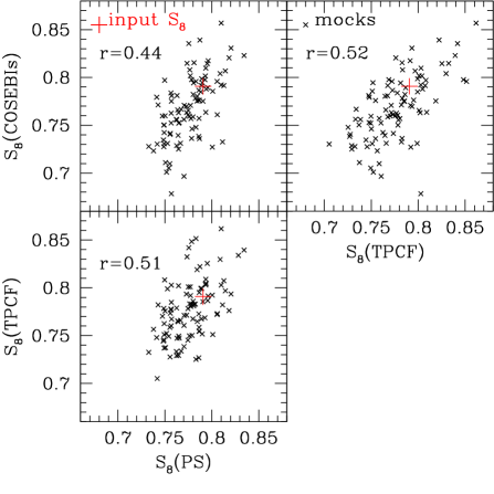
Figure 12: Scatter plots showing median values of marginalized one-dimensional posterior distributions of $S_{8}$ derived from cosmological analyses on 100 mock catalogs. In each of three panels, results from any one of the PS, TPCF, or COSEBIs analysis are compared to those from either of the rest. The red cross shows the value of $S_{8}$ adopted in generating the mock catalogs. The cross correlation coefficient defined by equation (13) is denoted in each panel.

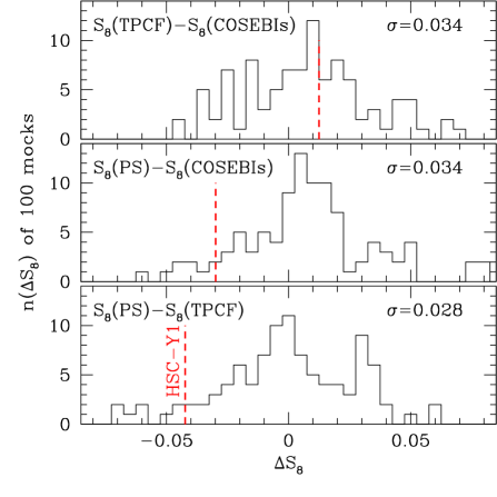
Figure 13: Frequency distributions of the differences in median $S_{8}$ values derived from any two of the PS, TPCF and COSEBIs analyses on 100 mock catalogs. The root-mean-square value of the distribution ($\sigma$) is denoted in each panel. Corresponding results from the real HSC-Y1 cosmic shear analyses are shown by the vertical red dashed line in each panel.

Finally, we compare the cosmological constraints from our fiducial model with HSC-Y1 cosmic shear PS (H19) and TPCF (H20) results. As seen in Figure 11, our constraint on $S_{8}$ is in good agreement with TPCF results (H20), and is in mild agreement with PS results (H19). Similar comparison results are found for two-dimensional constraint contours in $\Omega_{m}$-$\sigma_{8}$ plane presented in panel (a) of Figure 19, although our contours are much broader than theirs. Although no strong evidence of inconsistency among these results is seen from those results, we examine the consistency between them, paying particular attention to the fact that those analyses share the same HSC-Y1 data set with the same tomographic redshift binning and adopt a similar analysis setup.

We perform the same cross-correlation analysis as one done in H20 (see Section 6.7 of H20), in which cosmological inferences on the 100 realistic mock catalogs (see also Oguri et al., 2018) are performed with the same fiducial setups of HSC-Y1 PS and TPCF analyses except for ignoring PSF modeling errors because no PSF modeling error is added in the mock data, and then derived cosmological constraints are compared. We apply our COSEBIs analysis on the same mock catalogs but ignoring PSF modeling errors as well. We present the scatter plots comparing $S_{8}$ values (we take the median of a posterior distribution) derived from these three cosmological analyses on the same mock catalogs in Figure 12. We compute the standard cross-correlation coefficient of those distributions,

$$r(S_{8})={{\mbox{Cov}(S_{8}^{A},S_{8}^{B})}\over{{\mbox{Cov}(S_{8}^{A},S_{8}^{A})^{1/2}}{\mbox{Cov}(S_{8}^{B},S_{8}^{B})^{1/2}}}},$$ (13)

where the superscripts $A$ and $B$ stand for an analysis method (i.e., PS, TPCF or COSEBIs). We show the results in each panel of Figure 12. We find $r(S_{8})\sim 0.5$ for all the three cases, which indicates that the correlations between derived cosmological constraints among the three analyses are mild. Although qualitative, this result can be intuitively understood as each analysis method is sensitive to different multipole ranges, as seen in Figure 1. In Figure 13, we present frequency distributions of the differences in the $S_{8}$ values ($\Delta S_{8}=S_{8}^{A}-S_{8}^{B}$) derived from any pair of the PS, TPCF and COSEBIs analyses along with corresponding results from the real HSC-Y1 cosmic shear analyses (shown by the vertical red dashed line). We also compute the root-mean-square values of these distributions ($\sigma$) which are denoted in each panel. We find that derived $\sigma$ values for $\Delta S_{8}$ are only slightly smaller than ones for parents $S_{8}$ (0.022, 0.031, and 0.038 for PS, TPCF and COSEBIs, respectively), which confirms mild correlations between derived cosmological constraints among the three analyses. We note that similar results but for the COSEBIs, band power spectra, and TPCF analyses are found in KiDS-1000 cosmic shear study by Asgari et al. (2021). It follows from the above results that the $\Delta S_{8}$ values from three real HSC-Y1 cosmic shear analyses are explained by statistical fluctuations below 1.5$\sigma$.

7 Summary and conclusions

We have presented a cosmological analysis of the cosmic shear COSEBIs measured from the HSC-Y1 data, covering 136.9 deg². Photometric redshifts derived from the HSC five-band photometry are adopted to select galaxies and divided into four tomographic redshift bins ranging from $z=0.3$ to $1.5$ with equal widths of $\Delta z=0.3$. The total number of selected galaxies is 9.6 million. We compute tomographic E/B-mode COSEBIs from measured cosmic shear TPCFs on the angular range of $4\arcmin<\theta<180\arcmin$.

In addition to the HSC-Y1 data set, we have used HSC-Y1 mock shape catalogs constructed from full-sky gravitational lensing simulations (Takahashi et al., 2017) that fully take account of the survey geometry and measurement noise (Shirasaki et al., 2019). Using 2268 mock realizations, we have derived the E/B-mode covariance matrices adopted in our cosmological analysis. The mock catalogs are also used to assess the statistical significance of some of our results.

We have quantitatively tested the consistency of the B-mode COSEBIs signals with zero using the standard $\chi^{2}$ statistics, and found $\chi^{2}=66.1$ for 50 degrees-of-freedom, corresponding to the $p$-value of 0.063. We thus conclude that no evidence of significant B-mode shear is found.

We have performed a standard Bayesian likelihood analysis for the cosmological inference of the measured E-mode COSEBIs. Our fiducial $\Lambda$CDM model consists of five cosmological parameters and includes contributions from intrinsic alignment of galaxies (with 2 parameters for the nonlinear alignment IA model) as well as six nuisance parameters (1 for PSF errors, 1 for shear calibration error, and 4 for source redshift distribution errors). We have found that our fiducial model fits the measured E-mode COSEBIs signals very well with a minimum $\chi^{2}$ of 40.7 for 47 effective degrees-of-freedom. Derived marginalized one-dimensional constraint on $S_{8}$ is $S_{8}=0.809_{-0.026}^{+0.036}$ (mean and 68% credible interval).

We have carefully checked the robustness of our cosmological results against astrophysical uncertainties in modeling and systematics uncertainties in measurements. The former includes the intrinsic alignment of galaxies and the baryonic feedback effect on the nonlinear matter power spectrum, and the latter includes PSF errors, shear calibration error, errors in the estimation of source redshift distributions, and a residual constant shear over fields. We have tested the validity of our treatment of those uncertainties by changing parameter setups or by adopting empirical or extreme models for them. We have found that none of these uncertainties has a significant impact on the cosmological constraints. We have also confirmed the internal consistency of our results among different choices of tomographic redshift bins and different scale-cuts.

We have examined, using mock HSC-Y1 catalogs, the consistency in the $S_{8}$ constraints derived from the three HSC-Y1 cosmic shear two-point statistics, the PS (H19), TPCF (H20), and COSEBIs (this study), which share the same HSC-Y1 data set with the same tomographic redshift binning and adopt a similar analysis setup. We have found that correlations between derived $S_{8}$ constraints among the three analyses are mild, most likely because each analysis method is sensitive to different multipole ranges of cosmic shear power spectra. We have also found that differences in the derived $S_{8}$ values between different analyses are explained by statistical fluctuations below 1.5$\sigma$.

We have compared our $S_{8}$ constraint with those obtained from DES-Y3 (Amon et al., 2022) and KiDS-1000 (Asgari et al., 2021). We have found that our $S_{8}$ value is higher than theirs such that 68% credible intervals only slightly overlap with each other at the edges. Quantitatively, $S_{8}$ constraint from DES-Y3 (their $\Lambda$CDM-Optimized model) is in about 1.0$\sigma$ difference, and that of KiDS-1000 (their COSEBIs result) is in about 1.4$\sigma$ difference from our fiducial result (see Figure 11). We have also found that the $S_{8}$ constraint from Planck (Planck Collaboration et al., 2020a) is consistent with our result.

We would like to thank the anonymous referee for many constructive comments on the earlier manuscript which improved the paper. We would like to thank members of the HSC weak lensing working group for useful discussions. We would like to thank R. Takahashi for making full-sky gravitational lensing simulation data publicity available. We would like to thank Martin Kilbinger for making the software Athena publicly available, Antony Lewis and Anthony Challinor for making the software CAMB publicly available, MultiNest developers for MultiNest publicly available, HEALPix team for HEALPix software publicity available, and Nick Kaiser for making the software imcat publicly available.

This work was supported in part by JSPS KAKENHI Grant Number JP15H05892, JP17K05457, JP20H05856, JP20H00181 and 22K03655.

Data analysis were in part carried out on PC cluster at Center for Computational Astrophysics, National Astronomical Observatory of Japan. Numerical computations were in part carried out on Cray XC30 and XC50 at Center for Computational Astrophysics, National Astronomical Observatory of Japan, and also on Cray XC40 at YITP in Kyoto University.

The Hyper Suprime-Cam (HSC) collaboration includes the astronomical communities of Japan and Taiwan, and Princeton University. The HSC instrumentation and software were developed by the National Astronomical Observatory of Japan (NAOJ), the Kavli Institute for the Physics and Mathematics of the Universe (Kavli IPMU), the University of Tokyo, the High Energy Accelerator Research Organization (KEK), the Academia Sinica Institute for Astronomy and Astrophysics in Taiwan (ASIAA), and Princeton University. Funding was contributed by the FIRST program from the Japanese Cabinet Office, the Ministry of Education, Culture, Sports, Science and Technology (MEXT), the Japan Society for the Promotion of Science (JSPS), Japan Science and Technology Agency (JST), the Toray Science Foundation, NAOJ, Kavli IPMU, KEK, ASIAA, and Princeton University.

This paper is based on data collected at the Subaru Telescope and retrieved from the HSC data archive system, which is operated by Subaru Telescope and Astronomy Data Center (ADC) at NAOJ. Data analysis was in part carried out with the cooperation of Center for Computational Astrophysics (CfCA) at NAOJ. We are honored and grateful for the opportunity of observing the Universe from Maunakea, which has the cultural, historical and natural significance in Hawaii.

This paper makes use of software developed for Vera C. Rubin Observatory. We thank the Rubin Observatory for making their code available as free software at http://pipelines.lsst.io/.

The Pan-STARRS1 Surveys (PS1) and the PS1 public science archive have been made possible through contributions by the Institute for Astronomy, the University of Hawaii, the Pan-STARRS Project Office, the Max Planck Society and its participating institutes, the Max Planck Institute for Astronomy, Heidelberg, and the Max Planck Institute for Extraterrestrial Physics, Garching, The Johns Hopkins University, Durham University, the University of Edinburgh, the Queen’s University Belfast, the Harvard-Smithsonian Center for Astrophysics, the Las Cumbres Observatory Global Telescope Network Incorporated, the National Central University of Taiwan, the Space Telescope Science Institute, the National Aeronautics and Space Administration under grant No. NNX08AR22G issued through the Planetary Science Division of the NASA Science Mission Directorate, the National Science Foundation grant No. AST-1238877, the University of Maryland, Eotvos Lorand University (ELTE), the Los Alamos National Laboratory, and the Gordon and Betty Moore Foundation.

Appendix A Test of the measurements method of COSEBIs using mock catalogs

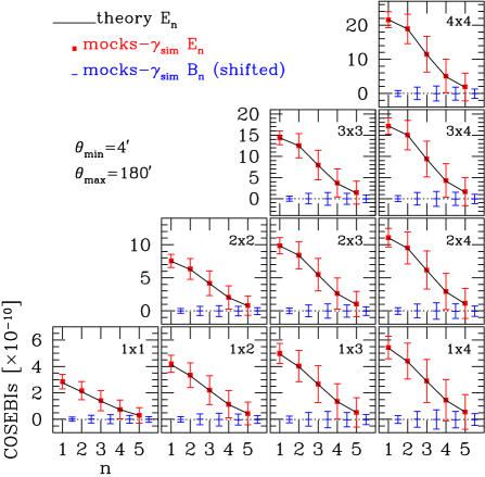
Figure 14: E/B-mode COSEBIs of the same redshift bin combinations as the HSC-Y1 measurements (shown in Figure 2) measured from HSC-Y1 mock catalogs are compared with the theoretical predictions. In these mock measurements, the cosmic shear signals without shape-noise components are used. Means and root-mean-squares (RMSs) of COSEBIs signals computed from 2268 HSC-Y1 mock catalogs are shown by red filled squares and blue bars for E- and B-mode, respectively. B-mode signals are shifted to right by 0.5 for clarify. The black lines show the theoretical predictions of E-mode COSEBIs based on WMAP9 cosmological model (Hinshaw et al., 2013) which is adopted in the ray-tracing simulation (Takahashi et al., 2017).

Here we present results of an accuracy test of our method of measuring COSEBIs signals, which is described in section 4.1. To do this, we use 2268 HSC-Y1 mock catalogs but ignoring shape-noise (Shirasaki et al., 2019). We measure E/B-mode COSEBIs from each of 2268 mock catalogs using the same method as the real HSC-Y1 COSEBIs measurements (see section 4.1), and compute means and root-mean-squares (RMSs) of them. Since the shape-noise is not included in this mock analysis, the RMSs represent an expected sample variance for the HSC-Y1 field. The results are shown in Figure 14 along with the theoretical predictions of E-mode COSEBIs based on WMAP9 cosmological model (Hinshaw et al., 2013), which is adopted in the ray-tracing simulation (Takahashi et al., 2017). It is seen from the figure that the averaged $E_{n}$ signals agree with the theoretical predictions well within the RMSs, and $B_{n}$ signals are consistent with zero. Therefore we conclude that the measurement method is accurate enough for this study.

Appendix B Estimations of COSEBIs signals from possible systematics

B.1 COSEBIs from shapes of PSF and residuals

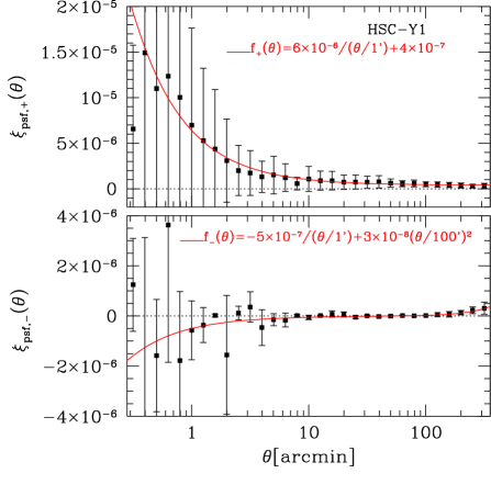
Figure 15: Symbols with error-bars show $\xi_{\mbox{psf},\pm}$ defined in equation (15) with measured $\xi_{\pm}^{pp}$, $\xi_{\pm}^{pq}$ and $\xi_{\pm}^{qq}$ from HSC-Y1 data set (see Appendix 2 of H20). Here $\alpha_{\mbox{psf}}=0.029\pm 0.010$ and $\beta_{\mbox{psf}}=-1.42\pm 1.11$ are adopted. Errors shown are computed from those of $\alpha_{\mbox{psf}}$ and $\beta_{\mbox{psf}}$. The solid curve show the fitting functions (see text for details).

Here we describe our scheme to estimate COSEBIs signals arising from residuals in the correction for the point spread function (PSF) anisotropy in galaxy shapes (see Mandelbaum, 2018, for a review), and present the result. In fact, systematic tests of the HSC-Y1 shape catalog showed small residual correlations between galaxy shears and PSF shapes (Mandelbaum et al., 2018a; Oguri et al., 2018), which may bias the cosmic shear COSEBIs and our cosmological analysis.

We first estimate TPCFs arising from PSF residuals following the scheme adopted in H20, which is based on the simple model used by H19 (see also Troxel et al., 2018). The model assumes that PSF residuals are added to the shear linearly

$$\gamma^{\mbox{sys}}=\alpha_{\mbox{psf}}\gamma^{p}+\beta_{\mbox{psf}}\gamma^{q},$$ (14)

where $\gamma^{P}$ is the shear of the shape of the model PSF, and $\gamma^{q}$ is the difference in shears between the PSF model and the true PSF, as estimated from the shapes of individual stars, $\gamma^{\ast}$, i.e., $\gamma^{q}=\gamma^{p}-\gamma^{\ast}$. The first and second terms of the right hand side of equation (14) represent the residual PSF effects from the deconvolution error and the imperfect PSF model, respectively. With these terms added to the measured shear $\hat{\gamma}$, the contributions from these terms to observed TPCFs are written as

$$\xi_{\mbox{psf},\pm}(\theta)=\alpha_{\mbox{psf}}^{2}\xi_{\pm}^{pp}(\theta)+2\alpha_{\mbox{psf}}\beta_{\mbox{psf}}\xi_{\pm}^{pq}(\theta)+\beta_{\mbox{psf}}^{2}\xi_{\pm}^{qq}(\theta),$$ (15)

where $\xi_{\pm}^{pp}$ and $\xi_{\pm}^{qq}$ represent the auto-TPCFs of $\gamma^{p}$ and $\gamma^{q}$, respectively, and $\xi_{\pm}^{pq}$ are the cross-TPCFs of $\gamma^{p}$ and $\gamma^{q}$. Those TPCFs measured from HSC-Y1 data are presented in Figures 20 and 23 of H20, for $\xi_{+}$ and $\xi_{-}$, respectively. The model parameters, $\alpha_{\mbox{psf}}$ and $\beta_{\mbox{psf}}$, can be estimated by the cross correlation functions between $\gamma^{p,q}$ and galaxy shears, $\xi^{gp,gq}=\langle\hat{\gamma}\gamma^{p,q}\rangle$, which are related to $\xi_{\pm}^{pp,pq,qq}$ as

$$\xi_{\pm}^{gp} = \alpha_{\mbox{psf}}\xi_{\pm}^{pp}+\beta_{\mbox{psf}}\xi_{\pm}^{pq},$$ (16)

$$\xi_{\pm}^{gq} = \alpha_{\mbox{psf}}\xi_{\pm}^{pq}+\beta_{\mbox{psf}}\xi_{\pm}^{qq}.$$ (17)

In measuring these quantities, we use the combined galaxy catalog of the four tomographic redshift bins, because the measurement of $\xi_{-}^{gp,gq}$ is very noisy as shown in Figure 19 of H20. As a consequence, we do not take into account possible redshift dependence of $\alpha_{\mbox{psf}}$ and $\beta_{\mbox{psf}}$. For $\xi_{+}$ component, the derived $\alpha_{\mbox{psf}}$ and $\beta_{\mbox{psf}}$ with equations (16) and (17) are shown in Figure 21 of H20, and their means and standard deviations were found to be $\alpha_{\mbox{psf}}=0.029\pm 0.010$ and $\beta_{\mbox{psf}}=-1.42\pm 1.11$ (H20). For $\xi_{-}$ component, due to very poor signal-to-noise ratios of the TPCFs (see Figures 19 and 23 of H20), useful estimated values of $\alpha_{\mbox{psf}}$ and $\beta_{\mbox{psf}}$ could not be derived (see Appendix 2 of H20), and thus in the following analysis we adopt the values obtained from $\xi_{+}$ component for $\xi_{-}$ component. In Figure 15, $\xi_{\mbox{psf},\pm}$ defined in equation (15) with $\alpha_{\mbox{psf}}=0.029\pm 0.010$ and $\beta_{\mbox{psf}}=-1.42\pm 1.11$ are shown, where error bars are computed from those of $\alpha_{\mbox{psf}}$ and $\beta_{\mbox{psf}}$. We derived the fitting functions of those estimates over the $\theta$-range of our interest as (plotted as solid curves in Figure 15)

$$\xi_{\mbox{psf},+}^{\rm fit}(\theta) = 6\times 10^{-6}\left({\theta\over{1^{\prime}}}\right)^{-1}+4\times 10^{-7},$$ (18)

$$\xi_{\mbox{psf},-}^{\rm fit}(\theta) = -5\times 10^{-7}\left({\theta\over{1^{\prime}}}\right)^{-1}+3\times 10^{-8}\left({\theta\over{100^{\prime}}}\right)^{2}.$$ (19)

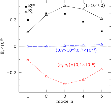
Figure 16: Filled squares show E-mode COSEBIs signals expected from PSF residuals in HSC-Y1 shape catalog (see Appendix B.1 for details). Crosses show E-mode COSEBIs signals arising from a constant shear of $|c|=10^{-3}$ on positions of galaxies used in this study (see Appendix B.2 for details). Results for three cases are plotted; $(c_{1},c_{2})=(10^{-3},0)$, $(0,10^{-3})$, and $(1/\sqrt{2}\times 10^{-3},1/\sqrt{2}\times 10^{-3})$ for the solid, dashed, and long-dashed line, respectively. Here results of tomographic redshift bins of $z_{3}\times z_{3}$ are shown, but results are insensitive to a choice of bins.

Using the above fitting functions, we derived E-mode COSEBIs expected from PSF residuals using equation (2) with the same scale-cut ($4\arcmin<\theta<180\arcmin$) as one adopted in our cosmological analysis. The result is shown in Figure 16 as filled squares. Although the derived E-mode COSEBIs should be considered as a rough estimate because it is based on the simple linear model, equations (14) and (15) with $\alpha_{\mbox{psf}}$ and $\beta_{\mbox{psf}}$ being not well determined, we may expect that it captures its characteristic shape. Therefore, in our cosmological analysis, we take this result as a reference model, $E_{n}^{\rm psf-ref}$, and introduce an amplitude parameter as

$$E_{n}^{\rm psf}=A_{\rm psf}E_{n}^{\rm psf-ref}.$$ (20)

We add this term to the theoretical prediction for the E-mode COSEBIs. We treat $A_{\rm psf}$ as a nuisance parameter (see Section 5.1.3).

B.2 COSEBIs from the constant shear over a field

The value of the shear averaged over a field is not expected to be zero due to the presence of the cosmic shear signal on scales larger than a field. However, it could also be non-zero due to residual systematics in the shear estimation and/or data reduction process. The latter, if present, may bias the cosmological inference. Mandelbaum et al. (2018a) examined a mean shear of the HSC-Y1 shape catalog, and found no evidence of a mean shear above that expected from large-scale cosmic shear. H20 reexamined it for each tomographic galaxy sample and for each field, and found that measured mean shears are consistent with that expected from large-scale cosmic shear (see Appendix 1 of H20). Although, as just mentioned above, no clear evidence of an excess mean shear was found, we check the impact of a constant shear over a field on our cosmological analysis by modeling it as a redshift-independent constant shear for simplicity, which we describe below.

COSEBIs signals arising from a constant shear were studies in detail in Appendix D of Asgari et al. (2021) that we follow here. We denote two components of a constant shear in the Cartesian coordinates as $(c_{1},c_{2})$. A constant shear generates a separation-independent constant $\xi_{+}$ term (to be specific, $\xi_{+}^{c}=c_{1}^{2}+c_{2}^{2}$), and a separation-dependent $\xi_{-}^{c}$ term, whose shape is determined by a field geometry and masks (see equation (D.3) of Asgari et al. (2021)). In the transformation from TPCFs to COSEBIs, equation (2), the constant $\xi_{+}^{c}$ term is filtered out, only $\xi_{-}^{c}$ term remains, and E-mode COSEBIs is given by equation (D.6) of Asgari et al. (2021),

$$E_{n}^{c} = {1\over 2}(c_{1}^{2}-c_{2}^{2})\int_{\theta_{\rm min}}^{\theta_{\rm max}}d\theta~{}\theta T_{-n}\langle\cos(4\phi)\rangle(\theta)$$ (21)

$$+c_{1}c_{2}\int_{\theta_{\rm min}}^{\theta_{\rm max}}d\theta~{}\theta T_{-n}\langle\sin(4\phi)\rangle(\theta),$$

where $\phi$ is the polar angle of the vector connecting two galaxies in the Cartesian coordinates, and $\langle...\rangle(\theta)$ denotes the average taken over all pairs of galaxies with a separation $\theta$.

We estimate actual $E_{n}^{c}$ signals for HSC-Y1 shear catalog with $|c|=10^{-3}$ (which is a typical value of HSC-Y1 shear catalog, see Figure 18 of H20) by artificially assigning a constant shear of $(c_{1},c_{2})$ (but in the sky coordinates, see a discussion below on this point) to all the galaxies, and doing the same COSEBIs measurement procedure as done for the real data. The results are shown in Figure 16 for three cases; $(c_{1},c_{2})=(10^{-3},0)$, $(0,10^{-3})$, and $(1/\sqrt{2}\times 10^{-3},1/\sqrt{2}\times 10^{-3})$ for the solid, dashed, and long-dashed line, respectively. In the plot, results of tomographic redshift bins of $z_{3}\times z_{3}$ are shown, but are insensitive to a choice of bins. It is found from these results that the first term of equation (21) is much larger than the second term except for cases of $|c_{1}|\simeq|c_{2}|$ though $E_{n}^{c}$ itself is very small in such cases. Note that from equation (21), one may expect that $|E_{n}^{c}|$ for cases of $(c_{1},c_{2})=(10^{-3},0)$ and $(0,10^{-3})$ should be equal, but not exactly in those actual measurements as can be seen in Figure 16. The reason for this is our use of the sky coordinates, instead of the Cartesian coordinates, in assigning a constant shear; we simply replace shears of HSC shape catalog which are defined in the sky coordinates with a constant shear $(c_{1},c_{2})$. In this case, equation (21) does not hold, but is still useful to understand a basic behavior of $E_{n}^{c}$ as each of 6 HSC-Y1 fields is not very wide, and 5 out of 6 fields have a strip-shaped geometry on the equator (see Figure 1 of Mandelbaum et al. (2018a)).

Our modeling of E-mode COSEBIs arising from the constant shear, which we use to check the impact of a constant shear on our cosmological analysis, is as follows: We consider a redshift-independent constant shear for simplicity (see Appendix 1 of H20 for a discussion on this point). From the above analysis, we find that the first term of equation (21) dominates $E_{n}^{c}$ signals, and thus it may be reasonable to adopt the measured $E_{n}^{c}$ for the case of $(c_{1},c_{2})=(10^{-3},0)$ as a reference for modeling. We denote it as $E_{n}^{c-\rm ref}$, and introduce an amplitude parameter as

$$E_{n}^{\langle\gamma\rangle}=A_{\langle\gamma\rangle}E_{n}^{c-\rm ref}.$$ (22)

We add this term to the theoretical prediction for the E-mode COSEBIs. We treat $A_{\langle\gamma\rangle}$ as a nuisance parameter (see Section 5.1.3).

Appendix C Supplementary figures

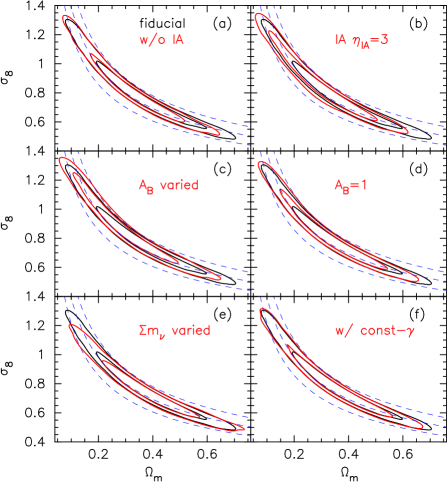
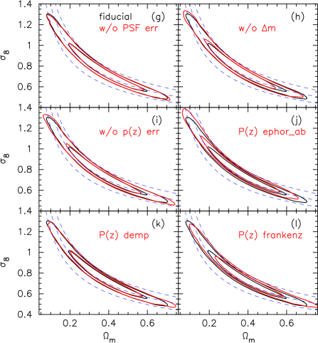
Figure 17: Comparison of constraints in the $\Omega_{m}$-$\sigma_{8}$ plane between the fiducial setup (black contours) and different assumptions, as described in the text (red contours showing 68% and 95% credible levels). Dashed blue curves show constant $S_{8}$ loci ($S_{8}=0.7$, 0.8 and 0.9 from bottom to top, respectively).

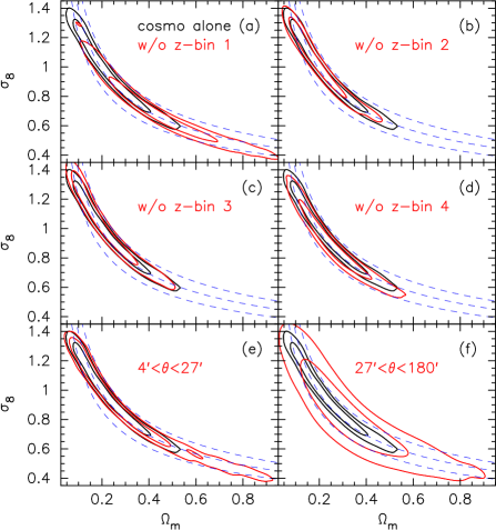
Figure 18: Comparison of constraints in the $\Omega_{m}$-$\sigma_{8}$ plane from the cosmology alone setup (black contours) with different setups for internal consistency checks (red contours showing 68% and 95% credible levels). Dashed blue curves show constant $S_{8}$ loci ($S_{8}=0.7$, 0.8 and 0.9 from bottom to top, respectively).

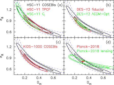
Figure 19: Marginalized posterior contours (68% and 95% credible levels) in the $\Omega_{m}$-$\sigma_{8}$ plane. Our result from the fiducial $\Lambda$CDM model (black contours) is compared with results in the literature (red- or green-line contours): (A) HSC-Y1 cosmic shear TPCF (red lines, H20) and PS results (green lines, H19). (b) Dark Energy Survey Year 1 (DES-Y1) cosmic shear TPCF result (Troxel et al., 2018). Note that in Section 6.5, we take $S_{8}$ constraint from DES-Y3 result (Amon et al., 2022), but its chain is not yet available. (c) KiDS-1000 cosmic shear COSEBIs result (Asgari et al., 2021). (d) Planck 2018 CMB result without CMB lensing (Planck Collaboration et al., 2020a, TT+TE+EE+lowE, red lines), and Planck 2018 lensing result (Planck Collaboration et al., 2020b, green lines). Dashed blue curves show constant $S_{8}$ loci ($S_{8}=0.7$, 0.8 and 0.9 from bottom to top, respectively).

In this Appendix, we present supplementary figures for systematics tests (Section 6.2), internal consistency checks (Section 6.3), and comparison of our cosmological constraints with ones from other projects (Section 6.5). Although in those sections we use $S_{8}=\sigma_{8}(\Omega_{m}/0.3)^{\alpha}$ with $\alpha=0.5$ for a primary parameter to be constrained by cosmic shear two-point statistics, a single choice of $\alpha$ does not always provide an optimal description for the $\sigma_{8}$-$\Omega_{m}$ degeneracy, especially for cases with broad confidence contours such as ours. Therefore, in this Appendix, we present marginalized posterior contours in the $\Omega_{m}$-$\sigma_{8}$ plane.

In Figure 17, we compare constraints from our fiducial setup with different setups for systematics tests (see Section 6.2 for details). Figure 18 shows the same comparison but between the cosmology alone setup and different setups for internal consistency checks (see Section 6.3).

In Figure 19, we compare constraints from our fiducial $\Lambda$CDM model with other results in the literature (see Section 6.5), where constraints from other studies are derived from publicly available chains. Note that although different studies adopt different priors, we do not adjust them to our fiducial setup, but rather use their original priors. Therefore, part of the difference in the posteriors may be due to the different choices of priors and modeling.

There is one thing to note about panel (d) of Figure 19; we compare our result with Planck 2018 lensing result (Planck Collaboration et al., 2020b), which is not discussed in the main text because it does not provide a useful constraint on $S_{8}=\sigma_{8}(\Omega_{m}/0.3)^{0.5}$ but provides a tight constraint on $\sigma_{8}\Omega_{m}^{0.25}$ due to a different degeneracy direction in $\Omega_{m}$-$\sigma_{8}$ plane as can be seen from the panel (d). The cosmic microwave background (CMB) lensing is a unique probe of the distribution of mass in the Universe at intermediate redshifts (typically $z\sim 2$) and is thus complementary to cosmic shear statistics as is demonstrated in Planck Collaboration et al. (2020b). Such complementarity can also be seen in the panel (d), although a combined cosmological inference with Planck results is beyond the scope of this study.

References

- Aihara et al. (2018a) Aihara, H., Armstrong, R., Bickerton, S., et al. 2018a, PASJ, 70, S8
- Aihara et al. (2018b) Aihara, H., Arimoto, N., Armstrong, R., et al. 2018b, PASJ, 70, S4
- Amon et al. (2022) Amon, A., Gruen, D., Troxel, M. A., et al. 2022, Phys. Rev. D, 105, 023514
- Anderson (2003) Anderson, T. W. 2003, An introduction to multivariate statistical analysis, 3rd edn. (Wiley-Interscience)
- Asgari et al. (2017) Asgari, M., Heymans, C., Blake, C., et al. 2017, MNRAS, 464, 1676
- Asgari et al. (2012) Asgari, M., Schneider, P., & Simon, P. 2012, A&A, 542, A122
- Asgari et al. (2020) Asgari, M., Tröster, T., Heymans, C., et al. 2020, A&A, 634, A127
- Asgari et al. (2021) Asgari, M., Lin, C.-A., Joachimi, B., et al. 2021, A&A, 645, A104
- Barreira et al. (2018) Barreira, A., Krause, E., & Schmidt, F. 2018, J. Cosmology Astropart. Phys, 2018, 053
- Bird et al. (2012) Bird, S., Viel, M., & Haehnelt, M. G. 2012, MNRAS, 420, 2551
- Bridle & King (2007) Bridle, S., & King, L. 2007, New Journal of Physics, 9, 444
- Camacho et al. (2021) Camacho, H., Andrade-Oliveira, F., Troja, A., et al. 2021, arXiv e-prints, arXiv:2111.07203
- Challinor & Lewis (2011) Challinor, A., & Lewis, A. 2011, Phys. Rev. D, 84, 043516
- Chisari et al. (2018) Chisari, N. E., Richardson, M. L. A., Devriendt, J., et al. 2018, MNRAS, 480, 3962
- Dark Energy Survey Collaboration et al. (2016) Dark Energy Survey Collaboration, Abbott, T., Abdalla, F. B., et al. 2016, MNRAS, 460, 1270
- de Jong et al. (2013) de Jong, J. T. A., Verdoes Kleijn, G. A., Kuijken, K. H., & Valentijn, E. A. 2013, Experimental Astronomy, 35, 25
- Feroz & Hobson (2008) Feroz, F., & Hobson, M. P. 2008, MNRAS, 384, 449
- Feroz et al. (2009) Feroz, F., Hobson, M. P., & Bridges, M. 2009, MNRAS, 398, 1601
- Feroz et al. (2019) Feroz, F., Hobson, M. P., Cameron, E., & Pettitt, A. N. 2019, The Open Journal of Astrophysics, 2, 10
- Hamana et al. (2020) Hamana, T., Shirasaki, M., Miyazaki, S., et al. 2020, PASJ, 72, 16
- Harnois-Déraps et al. (2015) Harnois-Déraps, J., van Waerbeke, L., Viola, M., & Heymans, C. 2015, MNRAS, 450, 1212
- Hartlap et al. (2007) Hartlap, J., Simon, P., & Schneider, P. 2007, A&A, 464, 399
- Hellwing et al. (2016) Hellwing, W. A., Schaller, M., Frenk, C. S., et al. 2016, MNRAS, 461, L11
- Hikage et al. (2019) Hikage, C., Oguri, M., Hamana, T., et al. 2019, PASJ, 71, 43
- Hildebrandt et al. (2017) Hildebrandt, H., Viola, M., Heymans, C., et al. 2017, MNRAS, 465, 1454
- Hildebrandt et al. (2020) Hildebrandt, H., Köhlinger, F., van den Busch, J. L., et al. 2020, A&A, 633, A69
- Hinshaw et al. (2013) Hinshaw, G., Larson, D., Komatsu, E., et al. 2013, ApJS, 208, 19
- Hirata & Seljak (2003) Hirata, C., & Seljak, U. 2003, MNRAS, 343, 459
- Hirata & Seljak (2004) Hirata, C. M., & Seljak, U. 2004, Phys. Rev. D, 70, 063526
- Ilbert et al. (2009) Ilbert, O., Capak, P., Salvato, M., et al. 2009, ApJ, 690, 1236
- Joachimi et al. (2011) Joachimi, B., Mandelbaum, R., Abdalla, F. B., & Bridle, S. L. 2011, A&A, 527, A26
- Kilbinger (2015) Kilbinger, M. 2015, Reports on Progress in Physics, 78, 086901
- Kirk et al. (2015) Kirk, D., Brown, M. L., Hoekstra, H., et al. 2015, Space Sci. Rev., 193, 139
- Köhlinger et al. (2017) Köhlinger, F., Viola, M., Joachimi, B., et al. 2017, MNRAS, 471, 4412
- Laigle et al. (2016) Laigle, C., McCracken, H. J., Ilbert, O., et al. 2016, ApJS, 224, 24
- Lesgourgues et al. (2013) Lesgourgues, J., Mangano, G., Miele, G., & Pastor, S. 2013, Neutrino Cosmology
- Mandelbaum (2018) Mandelbaum, R. 2018, ARA&A, 56, 393
- Mandelbaum et al. (2018a) Mandelbaum, R., Miyatake, H., Hamana, T., et al. 2018a, PASJ, 70, S25
- Mandelbaum et al. (2018b) Mandelbaum, R., Lanusse, F., Leauthaud, A., et al. 2018b, MNRAS, 481, 3170
- McCarthy et al. (2017) McCarthy, I. G., Schaye, J., Bird, S., & Le Brun, A. M. C. 2017, MNRAS, 465, 2936
- Mead et al. (2015) Mead, A. J., Peacock, J. A., Heymans, C., Joudaki, S., & Heavens, A. F. 2015, MNRAS, 454, 1958
- Oguri et al. (2018) Oguri, M., Miyazaki, S., Hikage, C., et al. 2018, PASJ, 70, S26
- Planck Collaboration et al. (2020a) Planck Collaboration, Aghanim, N., Akrami, Y., et al. 2020a, A&A, 641, A6
- Planck Collaboration et al. (2020b) —. 2020b, A&A, 641, A8
- Raveri & Hu (2019) Raveri, M., & Hu, W. 2019, Phys. Rev. D, 99, 043506
- Schaye et al. (2010) Schaye, J., Dalla Vecchia, C., Booth, C. M., et al. 2010, MNRAS, 402, 1536
- Schneider et al. (2010) Schneider, P., Eifler, T., & Krause, E. 2010, A&A, 520, A116
- Schneider et al. (2002) Schneider, P., van Waerbeke, L., Kilbinger, M., & Mellier, Y. 2002, A&A, 396, 1
- Shirasaki et al. (2019) Shirasaki, M., Hamana, T., Takada, M., Takahashi, R., & Miyatake, H. 2019, MNRAS, 486, 52
- Smith et al. (2003) Smith, R. E., Peacock, J. A., Jenkins, A., et al. 2003, MNRAS, 341, 1311
- Springel et al. (2018) Springel, V., Pakmor, R., Pillepich, A., et al. 2018, MNRAS, 475, 676
- Takahashi et al. (2017) Takahashi, R., Hamana, T., Shirasaki, M., et al. 2017, ApJ, 850, 24
- Takahashi et al. (2012) Takahashi, R., Sato, M., Nishimichi, T., Taruya, A., & Oguri, M. 2012, ApJ, 761, 152
- Tanaka et al. (2018) Tanaka, M., Coupon, J., Hsieh, B.-C., et al. 2018, PASJ, 70, S9
- Troxel & Ishak (2015) Troxel, M. A., & Ishak, M. 2015, Phys. Rep., 558, 1
- Troxel et al. (2018) Troxel, M. A., MacCrann, N., Zuntz, J., et al. 2018, Phys. Rev. D, 98, 043528
- van Daalen et al. (2011) van Daalen, M. P., Schaye, J., Booth, C. M., & Dalla Vecchia, C. 2011, MNRAS, 415, 3649