AIM: An Adaptive and Iterative Mechanism for
Differentially Private Synthetic Data

Abstract.

We propose AIM, a novel algorithm for differentially private synthetic data generation. AIM is a workload-adaptive algorithm, within the paradigm of algorithms that first selects a set of queries, then privately measures those queries, and finally generates synthetic data from the noisy measurements. It uses a set of innovative features to iteratively select the most useful measurements, reflecting both their relevance to the workload and their value in approximating the input data. We also provide analytic expressions to bound per-query error with high probability, which can be used to construct confidence intervals and inform users about the accuracy of generated data. We show empirically that AIM consistently outperforms a wide variety of existing mechanisms across a variety of experimental settings.

1. Introduction

Differential privacy (Dwork et al., 2006) has grown into the preferred standard for privacy protection, with significant adoption by both commercial and governmental enterprises. Many common computations on data can be performed in a differentially private manner, including aggregates, statistical summaries, and the training of a wide variety predictive models. Yet one of the most appealing uses of differential privacy is the generation of synthetic data, which is a collection of records matching the input schema, intended to be broadly representative of the source data. Differentially private synthetic data is an active area of research  (Zhang et al., 2017; Chen et al., 2015; Zhang et al., 2019; Xu et al., 2017; Xie et al., 2018; Torfi et al., 2022; Vietri et al., 2020; Liu, 2016; Torkzadehmahani et al., 2019; Charest, 2011; Ge et al., 2021; Huang et al., [n.d.]; Jordon et al., 2019; Zhang et al., 2018; Tantipongpipat et al., 2019; Abay et al., 2018; Bindschaedler et al., 2017; Zhang et al., 2021; Asghar et al., 2019; Li et al., 2014) and has also been the basis for two competitions, hosted by the U.S. National Institute of Standards and Technology (Ridgeway et al., 2021).

Private synthetic data is appealing because it fits any data processing workflow designed for the original data, and, on its face, the user may believe they can perform any computation they wish, while still enjoying the benefits of privacy protection. Unfortunately it is well-known that there are limits to the accuracy that can be provided by synthetic data, under differential privacy or any other reasonable notion of privacy (Dinur and Nissim, 2003).

As a consequence, it is important to tailor synthetic data to some class of tasks, and this is commonly done by asking the user to provide a set of queries, called the workload, to which the synthetic data can be tailored. However, as our experiments will show, existing workload-aware techniques often fail to outperform workload-agnostic mechanisms, even when evaluated specifically on their target workloads. Not only do these algorithms fail to produce accurate synthetic data, they provide no way for end-users to detect the inaccuracy. As a result, in practical terms, differentially private synthetic data generation remains an unsolved problem.

In this work, we advance the state-of-the-art of differentially private synthetic data in two key ways. First, we propose a novel workload-aware mechanism that offers lower error than all competing techniques. Second, we derive analytic expressions to bound the per-query error of the mechanism with high probability.

Our mechanism, AIM, follows the select-measure-generate paradigm, which can be used to describe many prior approaches. Mechanisms following this paradigm first select a set of queries, then measure those queries in a differentially private way (through noise addition), and finally generate synthetic data consistent with the noisy measurements. We leverage Private-PGM (McKenna et al., 2019) for the generate step, as it provides a robust and efficient method for combining the noisy measurements into a single consistent representation from which records can be sampled.

The low error of AIM is primarily due to innovations in the select stage. AIM uses an iterative, greedy selection procedure, inspired by the popular MWEM algorithm for linear query answering. We define a highly effective quality score which determines the private selection of the next best marginal to measure. Through careful analysis, we define a low-sensitivity quality score that is able to take into account: (i) how well the candidate marginal is already estimated, (ii) the expected improvement measuring it can offer, (iii) the relevance of the marginal to the workload, and (iv) the available privacy budget. This novel quality score is accompanied by a host of other algorithmic techniques including adaptive selection of rounds and budget-per-round, intelligent initialization, and novel set of candidates from which to select.

In conjunction with AIM, we develop new techniques to quantify uncertainty in query answers derived from the generated synthetic data. The problem of error quantification for data independent mechanisms like the Laplace or Gaussian mechanism is trivial, as they provide unbiased answers with known variance to all queries. The problem is considerably more challenging for data-dependent mechanisms like AIM, where complex post-processing is performed and only a subset of workload queries have unbiased answers. Some mechanisms, like MWEM, provide theoretical guarantees on their worst-case error, under suitable assumptions. However, this is an a priori bound on error obtained from a theoretical analysis of the mechanism under worst-case datasets. Instead, we develop an a posteriori error analysis, derived from the intermediate differentially private measurements used to produce the synthetic data. Our error estimates therefore reflect the actual execution of AIM on the input data, but do not require any additional privacy budget for their calculation. Formally, our guarantees represent one-sided confidence intervals, and we refer to them simply as “confidence bounds”. To our knowledge, AIM is the only differentially private synthetic data generation mechanism that provides this kind of error quantification. This paper makes the following contributions:

1. In Section 3, we assess the prior work in the field, characterizing different approaches via key distinguishing elements and limitations, which brings clarity to a complex space.

2. In Section 4, we propose AIM, a new mechanism for synthetic data generation that is workload-aware (for workloads consisting of weighted marginals) as well as data-aware.

3. In Section 5, we derive analytic expressions to bound the per-query error of AIM with high probability. These expressions can be used to construct confidence bounds.

4. In Section 6, we conduct a comprehensive empirical evaluation, and show that AIM consistently outperforms all prior work, improving error over the next best mechanism by $1.6\times$ on average, and up to $5.7\times$ in some cases.

2. Background

In this section we provide relevant background and notation on datasets, marginals, and differential privacy required to understand this work.

2.1. Data, Marginals, and Workloads

Data

A dataset $D$ is a multiset of $N$ records, each containing potentially sensitive information about one individual. Each record $x\in D$ is a $d$-tuple $(x_{1},\dots,x_{d})$. The domain of possible values for $x_{i}$ is denoted by $\Omega_{i}$, which we assume is finite and has size $|\Omega_{i}|=n_{i}$. The full domain of possible values for $x$ is thus $\Omega=\Omega_{1}\times\dots\times\Omega_{d}$ which has size $\prod_{i}n_{i}=n$. We use $\mathcal{D}$ to denote the set of all possible datasets, which is equal to $\cup_{N=0}^{\infty}\Omega^{N}$.

Marginals

A marginal is a central statistic to the techniques studied in this paper, as it captures low-dimensional structure common in high-dimensional data distributions. A marginal for a set of attributes $r$ is essentially a histogram over $x_{r}$: it is a table that counts the number of occurrences of each $t\in\Omega_{r}$.

Definition 0 (Marginal).

Let $r\subseteq[d]$ be a subset of attributes, $\Omega_{r}=\prod_{i\in r}\Omega_{i}$, $n_{r}=|\Omega_{r}|$, and $x_{r}=(x_{i})_{i\in r}$. The marginal on $r$ is a vector $\mu\in\mathbb{R}^{n_{r}}$, indexed by domain elements $t\in\Omega_{r}$, such that each entry is a count, i.e., $\mu[t]=\sum_{x\in D}\mathbbm{1}[x_{r}=t]$. We let $M_{r}:\mathcal{D}\rightarrow\mathbb{R}^{n_{r}}$ denote the function that computes the marginal on $r$, i.e., $\mu=M_{r}(D)$.

In this paper, we use the term marginal query to denote the function $M_{r}$, and marginal to denote the vector of counts $\mu=M_{r}(D)$. With some abuse of terminology, we will sometimes refer to the attribute subset $r$ as a marginal query as well.

Workload

A workload is a collection of queries the synthetic data should preserve well. It represents the measure by which we will evaluate utility of different mechanisms. We want our mechanisms to take a workload as input, and adapt intelligently to the queries in it, providing synthetic data that is tailored to the queries of interest. In this work, we focus on the special (but common) case where the workload consists of a collection of weighted marginal queries. Our utility measure is stated in Definition 2.

Definition 0 (Workload Error).

A workload $W$ consists of a list of marginal queries $r_{1},\dots,r_{k}$ where $r_{i}\subseteq[d]$, together with associated weights $c_{i}\geq 0$. The error of a synthetic dataset $\hat{D}$ is defined as:

$$\text{Error}(D,\hat{D})=\frac{1}{k\cdot|D|}\sum_{i=1}^{k}c_{i}\left\lVert M_{r_{i}}(D)-M_{r_{i}}(\hat{D})\right\rVert_{1}$$

2.2. Differential privacy

Differential privacy protects individuals by bounding the impact any one individual can have on the output of an algorithm. This is formalized using the notion of neighboring datasets. Two datasets $D,D^{\prime}\in\mathcal{D}$ are neighbors (denoted $D\sim D^{\prime}$) if $D^{\prime}$ can be obtained from $D$ by adding or removing a single record.

Definition 0 (Differential Privacy).

A randomized mechanism ${\mathcal{M}}:\mathcal{D}\rightarrow\mathcal{R}$ satisfies $(\epsilon,\delta)$-differential privacy (DP) if for any neighboring datasets $D\sim D^{\prime}\in\mathcal{D}$, and any subset of possible outputs $S\subseteq\mathcal{R}$,

$$\Pr[{\mathcal{M}}(D)\in S]\leq\exp(\epsilon)\Pr[{\mathcal{M}}(D^{\prime})\in S]+\delta.$$

A key quantity needed to reason about the privacy of common randomized mechanisms is the sensitivity, defined below.

Definition 0 (Sensitivity).

Let $f:\mathcal{D}\rightarrow\mathbb{R}^{p}$ be a vector-valued function of the input data. The $L_{2}$ sensitivity of $f$ is
$\Delta(f)=\max_{D\sim D^{\prime}}\left\lVert f(D)-f(D^{\prime})\right\rVert_{2}$.

It is easy to verify that the $L_{2}$ sensitivity of any marginal query $M_{r}$ is $1$, regardless of the attributes in $r$. This is because one individual can only contribute a count of one to a single cell of the output vector. Below we introduce the two building block mechanisms used in this work.

Definition 0 (Gaussian Mechanism).

Let $f:\mathcal{D}\rightarrow\mathbb{R}^{p}$ be a vector-valued function of the input data. The Gaussian Mechanism adds i.i.d. Gaussian noise with scale $\sigma\Delta(f)$ to each entry of $f(D)$. That is,

$${\mathcal{M}}(D)=f(D)+\sigma\Delta(f)\mathcal{N}(0,\mathbb{I}),$$

where $\mathbb{I}$ is a $p\times p$ identity matrix.

Definition 0 (Exponential Mechanism).

Let $q_{r}:\mathcal{D}\rightarrow\mathbb{R}$ be quality score function defined for all $r\in\mathcal{R}$ and let $\epsilon\geq 0$ be a real number. Then the exponential mechanism outputs a candidate $r\in\mathcal{R}$ according to the following distribution:

$$\Pr[\mathcal{M}(D)=r]\propto\exp{\Big{(}\frac{\epsilon}{2\Delta}\cdot q_{r}(D)\Big{)}},$$

where $\Delta=\max_{r\in\mathcal{R}}\Delta(q_{r})$.

Our algorithm is defined using zCDP, an alternate version of differential privacy definition which offers beneficial composition properties. We convert to $(\epsilon,\delta)$ guarantees when necessary.

Definition 0 (zero-Concentrated Differential Privacy (zCDP)).

A randomized mechanism ${\mathcal{M}}$ is $\rho$-zCDP if for any two neighboring datasets $D$ and $D^{\prime}$, and all $\alpha\in(1,\infty)$, we have:

$$D_{\alpha}({\mathcal{M}}(D)\mid\mid{\mathcal{M}}(D^{\prime}))\leq\rho\cdot\alpha,$$

where $D_{\alpha}$ is the Rényi divergence of order $\alpha$.

Proposition 0 (zCDP of the Gaussian Mechanism (Bun and Steinke, 2016)).

The Gaussian Mechanism satisfies $\frac{1}{2\sigma^{2}}$-zCDP.

Proposition 0 (zCDP of the Exponential Mechanism (Cesar and Rogers, 2021)).

The Exponential Mechanism satisfies $\frac{\epsilon^{2}}{8}$-zCDP.

We rely on the following propositions to reason about multiple adaptive invocations of zCDP mechanisms, and the translation from zCDP to $(\epsilon,\delta)$-DP. The proposition below covers 2-fold adaptive composition of zCDP mechanisms, and it can be inductively applied to obtain analogous k-fold adaptive composition guarantees.

Proposition 0 (Adaptive Composition of zCDP Mechanisms (Bun and Steinke, 2016)).

Let ${\mathcal{M}}_{1}:\mathcal{D}\rightarrow\mathcal{R}_{1}$ be $\rho_{1}$-zCDP and ${\mathcal{M}}_{2}:\mathcal{D}\times\mathcal{R}_{1}\rightarrow\mathcal{R}_{2}$ be $\rho_{2}$-zCDP. Then the mechanism ${\mathcal{M}}={\mathcal{M}}_{2}(D,{\mathcal{M}}_{1}(D))$ is $(\rho_{1}+\rho_{2})$-zCDP.

Proposition 0 (zCDP to DP (Canonne et al., 2020)).

If a mechanism ${\mathcal{M}}$ satisfies $\rho$-zCDP, it also satisfies $(\epsilon,\delta)$-differential privacy for all $\epsilon\geq 0$ and

$$\delta=\min_{\alpha>1}\frac{\exp{\big{(}(\alpha-1)(\alpha\rho-\epsilon)\big{)}}}{\alpha-1}\Big{(}1-\frac{1}{\alpha}\Big{)}^{\alpha}.$$

2.3. Private-PGM

An important component of our approach is a tool called Private-PGM (McKenna et al., 2019, 2021a; McKenna and Liu, 2022). For the purposes of this paper, we will treat Private-PGM as a black box that exposes an interface for solving subproblems important to our mechanism. We briefly summarize Private-PGM and three core utilities it provides. Private-PGM consumes as input a collection of noisy marginals of the sensitive data, in the format of a list of tuples $(\tilde{\mu}_{i},\sigma_{i},r_{i})$ for $i=1,\dots,k$, where $\tilde{\mu}_{i}=M_{r_{i}}(D)+\mathcal{N}(0,\sigma_{i}^{2}\mathbb{I})$.

Distribution Estimation

At the heart of Private-PGM is an optimization problem to find a distribution $\hat{p}$ that “best explains” the noisy observations $\tilde{\mu}_{i}$:

$$\hat{p}\in\operatorname*{argmin}_{p\in\mathcal{S}}\sum_{i=1}^{k}\frac{1}{\sigma_{i}}\left\lVert M_{r_{i}}(p)-\tilde{\mu}_{i}\right\rVert_{2}^{2}$$

Here $\mathcal{S}=\{p\mid p(x)\geq 0\text{ and }\sum_{x\in\Omega}p(x)=n\}$ is the set of (scaled) probability distributions over the domain $\Omega$. When $\tilde{\mu_{i}}$ are corrupted with i.i.d. Gaussian noise, this is exactly a maximum likelihood estimation problem (McKenna et al., 2019, 2021a; McKenna and Liu, 2022). In general, convex optimization over the scaled probability simplex is intractable for the high-dimensional domains we are interested in. Private-PGM overcomes this curse of dimensionality by exploiting the fact that the objective only depends on $p$ through its marginals. The key observation is that one of the minimizers of this problem is a graphical model $\hat{p}_{\theta}$. The parameters $\theta$ provide a compact representation of the distribution $p$ that we can optimize efficiently.

Junction Tree Size

The time and space complexity of Private-PGM depends on the measured marginal queries in a nuanced way, the main factor being the size of the junction tree implied by the measured marginal queries (McKenna et al., 2021a, b). While understanding the junction tree construction is not necessary for this paper, it is important to note that Private-PGM exposes a callable function $\textsf{JT-SIZE}(r_{1},\dots,r_{k})$ that can be invoked to check how large a junction tree is. JT-SIZE is measured in megabytes, and the runtime of distribution estimation is roughly proportional to this quantity. If arbitrary marginals are measured, JT-SIZE can grow out of control, no longer fitting in memory, and leading to unacceptable runtime.

Synthetic Data Generation

Given an estimated model $\hat{p}$,
Private-PGM implements a routine for generating synthetic tabular data that approximately matches the given distribution. It achieves this with a randomized rounding procedure, which is a lower variance alternative to sampling from $\hat{p}$ (McKenna et al., 2021a).

3. Prior Work on Synthetic Data

In this section we survey the state of the field, describing basic elements of a good synthetic data mechanism, along with novelties of more sophisticated mechanisms. We focus our attention on marginal-based approaches to differentially private synthetic data in this section, as these have generally seen the most success in practical applications. These mechanisms include PrivBayes (Zhang et al., 2017), PrivBayes+PGM (McKenna et al., 2019), MWEM+PGM (McKenna et al., 2019), MST (McKenna et al., 2021a), PrivSyn (Zhang et al., 2021), RAP (Aydore et al., 2021), GEM (Liu et al., 2021a), and PrivMRF (Cai et al., 2021). We will review other related work in Section 8. We will begin with a formal problem statement:

Problem 1 (Workload Error Minimization).

Given a workload $W$, our goal is to design an $(\epsilon,\delta)$-DP synthetic data mechanism $\mathcal{M}:\mathcal{D}\rightarrow\mathcal{D}$ such that the expected error defined in Definition 2 is minimized.

3.1. The Select-Measure-Generate Paradigm

Algorithm 1 MWEM+PGM

  Input: Dataset $D$, workload $W$, privacy parameter $\rho$, rounds $T$

  Output: Synthetic Dataset $\hat{D}$

  Initialize $\hat{p}_{0}=\text{Uniform}[\mathcal{X}]$

  $\epsilon=2\sqrt{\rho/T}$

  $\sigma=\sqrt{T/\rho}$

  for $t=1,\dots,T$ do

     select $r_{t}\in W$ using exponential mechanism with $\epsilon$ budget:

$$q_{r}(D)=\left\lVert M_{r}(D)-M_{r}(\hat{p}_{t-1})\right\rVert_{1}-n_{r}$$

     measure marginal on $C$:

$$\tilde{\mu}_{t}=M_{r_{t}}(D)+\mathcal{N}(0,\sigma^{2}\mathbb{I})$$

     estimate data distribution using Private-PGM:

$$\hat{p_{t}}=\operatorname*{argmin}_{p\in S}\sum_{i=1}^{t}\left\lVert M_{r_{i}}(p)-y_{i}\right\rVert_{2}^{2}$$

  end for

  generate synthetic data $\hat{D}$ using Private-PGM:

  return $\hat{D}$

We begin by providing a broad overview of the basic approach employed by many differentially private mechanisms for synthetic data. These mechanisms all fit naturally into the select-measure-generate framework. This framework represents a class of mechanisms which can naturally be broken up into 3 steps: (1) select a set of queries, (2) measure those queries using a noise-addition mechanism, and (3) generate synthetic data that explains the noisy measurements well. We consider iterative mechanisms that alternate between the select and measure step to be in this class as well. Mechanisms within this class differ in their methodology for selecting queries, the noise mechanism used, and the approach to generating synthetic data from the noisy measurements.

MWEM+PGM, shown in Algorithm 1, is one mechanism from this class that serves as a concrete example as well as the starting point for our improved mechanism, AIM. As the name implies, MWEM+PGM is a scalable instantiation of the well-known MWEM algorithm (Hardt et al., 2012) for linear query answering, where the multiplicative weights (MW) step is replaced by a call to Private-PGM. It is a greedy, iterative mechanism for workload-aware synthetic data generation, and there are several variants. One variant is shown in Algorithm 1. The mechanism begins by initializing an estimate of the joint distribution to be uniform over the data domain. Then, it runs for $T$ rounds, and in each round it does three things: (1) selects (via the exponential mechanism) a marginal query that is poorly approximated under the current estimate, (2) measures the selected marginal using the Gaussian mechanism, and (3) estimates a new data distribution (using Private-PGM) that explains the noisy measurements well. After $T$ rounds, the estimated distribution is used to generate synthetic tabular data. In the subsequent subsections, we will characterize existing mechanisms in terms of how they approach these different aspects of the problem.

3.2. Basic Elements of a Good Mechanism

In this section we outline some basic criteria reasonable mechanisms should satisfy to get good performance. These recommendations primarily apply to the measure step.

Measure Entire Marginals

Marginals are an appealing statistic to measure because every individual contributes a count of one to exactly one cell of the marginal. As a result, we can measure every cell of $M_{r}(D)$ at the same privacy cost of measuring a single cell. With a few exceptions ((Aydore et al., 2021; Liu et al., 2021a; Vietri et al., 2020)), existing mechanisms utilize this property of marginals or can be extended to use it. The alternative of measuring a single counting query at a time sacrifices utility unnecessarily.

Use Gaussian Noise.

Back of the envelope calculations reveal that if the number of measurements is greater than roughly $\log{(1/\delta)}\\ +\epsilon$, which is often the case, then the standard deviation of the required Gaussian noise is lower than that of the Laplace noise. Many newer mechanisms recognize this and use Gaussian noise, while older mechanisms were developed with Laplace noise, but can easily be adapted to use Gaussian noise instead.

Use Unbounded DP

For fixed $(\epsilon,\delta)$, the required noise magnitude is lower by a factor of $\sqrt{2}$ when using unbounded DP (add / remove one record) over bounded DP (modify one record). This is because the $L_{2}$ sensitivity of a marginal query $M_{r}$ is $1$ under unbounded DP, and $\sqrt{2}$ under bounded DP. Some mechanisms like MST, PrivSyn, and PrivMRF use unbounded DP, while other mechanisms like RAP, GEM, and PrivBayes use bounded DP. We remark that these two different definitions of DP are qualitatively different, and because of that, the privacy parameters have different interpretations. The $\sqrt{2}$ difference could be recovered in bounded DP by increasing the privacy budget appropriately.

3.3. Distinguishing Elements of Existing Work

Table 1. Taxonomy of select-measure-generate mechanisms.

Name	Year	Workload	Data	Budget	Efficiency
		Aware	Aware	Aware	Aware
Independent	-				✓
Gaussian	-	✓
PrivBayes (Zhang et al., 2017)	2014		✓	✓	✓
HDMM+PGM (McKenna et al., 2019)	2019	✓
PrivBayes+PGM (McKenna et al., 2019)	2019		✓	✓	✓
MWEM+PGM (McKenna et al., 2019)	2019	✓	✓
PrivSyn (Zhang et al., 2021)	2020		✓	✓	✓
MST (McKenna et al., 2021a)	2021		✓		✓
RAP (Aydore et al., 2021)	2021	✓	✓		✓
GEM (Liu et al., 2021a)	2021	✓	✓		✓
PrivMRF (Cai et al., 2021)	2021		✓	✓	✓
AIM [This Work]	2022	✓	✓	✓	✓

Beyond the basics, different mechanisms exhibit different novelties, and understanding the design considerations underlying the existing work can be enlightening. We provide a simple taxonomy of this space in Table 1 in terms of four criteria: workload-, data-, budget-, and efficiency-awareness. These characteristics primarily pertain to the select step of each mechanism.

Workload-awareness

Different mechanisms select from a different set of candidate marginal queries. PrivBayes and PrivMRF, for example, select from a particular subset of $k$-way marginals, determined from the data. Other mechanisms, like MST and PrivSyn, restrict the set of candidates to 2-way marginal queries. On the other end of the spectrum, the candidates considered by MWEM+PGM, RAP, and GEM, are exactly the marginal queries in the workload. This is appealing, since these mechanisms will not waste the privacy budget to measure marginals that are not relevant to the workload, however we show the benefit of extending the set of candidates beyond the workload.

Data-awareness

Many mechanisms select marginal queries from a set of candidates based on the data, and are thus data-aware. For example, MWEM+PGM selects marginal queries using the exponential mechanism with a quality score function that depends on the data. Independent, Gaussian, and HDMM+PGM are the exceptions, as they always select the same marginal queries no matter what the underlying data distribution is.

Budget-awareness

Another aspect of different mechanisms is how well do they adapt to the privacy budget available. Some mechanisms, like PrivBayes, PrivSyn, and PrivMRF recognize that we can afford to measure more (or larger) marginals when the privacy budget is sufficiently large. When the privacy budget is limited, these mechanisms recognize that fewer (and smaller) marginals should be measured instead. In contrast, the number and size of the marginals selected by mechanisms like MST, MWEM+PGM, RAP, and GEM does not depend on the privacy budget available.

Efficiency-awareness

Mechanisms that build on top of Private-PGM must take care when selecting measurements to ensure JT-SIZE remains sufficiently small to ensure computational tractability. Among these, PrivBayes+PGM, MST, and PrivMRF all have built-in heuristics in the selection criteria to ensure the selected marginal queries give rise to a tractable model. Gaussian, HDMM+PGM and MWEM+PGM have no such safeguards, and they can sometimes select marginal queries that lead to intractable models. In the extreme case, when the workload is all 2-way marginals, Gaussian selects all 2-way marginals, model required for Private-PGM explodes to the size of the entire domain, which is often intractable.

Mechanisms that utilize different techniques for post-processing noisy marginals into synthetic data, like PrivSyn, RAP, and GEM, do not have this limitation, and are free to select from a wider collection of marginals. While these methods do not suffer from this particular limitation of Private-PGM, they have other pros and cons which were surveyed in a recent article (McKenna and Liu, 2022).

Summary

With the exception of our new mechanism AIM, no mechanism listed in Table 1 is aware of all four factors we discussed. Mechanisms that do not have four checkmarks in Table 1 are not necessarily bad, but there are clear ways in which they can be improved. Conversely, mechanisms that have more checkmarks than other mechanisms are not necessarily better. For example, RAP has 3 checkmarks, but as we show in Section 6, it does not consistently beat Independent, which only has 1 checkmark.

3.4. Other Design Considerations

Beyond these four characteristics summarized in the previous section, different methods make different design decisions that are relevant to mechanism performance, but do not correspond to the four criteria discussed in the previous section. In this section, we summarize some of those additional design considerations.

Selection method

Some mechanisms select marginals to measure in a batch, while other mechanisms select them iteratively. Generally speaking, iterative methods like MWEM+PGM, RAP, GEM, and PrivMRF are preferable to batch methods, because the selected marginals will capture important information about the distribution that was not effectively captured by the previously measured marginals. On the other hand, PrivBayes, MST, and PrivSyn select all the marginals before measuring any of them. It is not difficult to construct examples where a batch method like PrivSyn has suboptimal behavior. For example, suppose the data contains three perfectly correlated attributes. We can expect iterative methods to capture the distribution after measuring any two 2-way marginals. On the other hand, a batch method like PrivSyn will determine that all three 2-way marginals need to be measured.

Budget split

Every mechanism in this discussion, except for PrivSyn, splits the privacy budget equally among selected marginals. This is a simple and natural thing to do, but it does not account for the fact that larger marginals have smaller counts that are less robust to noise, requiring a larger fraction of the privacy budget to answer accurately. PrivSyn provides a simple formula for dividing privacy budget among marginals of different sizes, but this approach is inherently tied to their batch selection methodology. It is much less clear how to divide the privacy budget within a mechanism that uses an iterative selection procedure.

Hyperparameters

All mechanisms have some hyperparameters than can be tuned to affect the behavior of the mechanism. Mechanisms like PrivBayes, MST, PrivSyn, and PrivMRF have reasonable default values for these hyperparameters, and these mechanisms can be expected to work well out of the box. On the other hand, MWEM+PGM, RAP, and GEM have to tune the number of rounds to run, and it is not obvious how to select this a priori. While the open source implementations may include a default value, the experiments conducted in the respective papers did not use these default values, in favor of non-privately optimizing over this hyper-parameter for each dataset and privacy level considered (Aydore et al., 2021; Liu et al., 2021a).

Algorithm 2 Initialize $p_{t}$ (subroutine of Algorithm 4)

1:  for $r\in\{r\in W_{+}\mid|r|=1\}$ do

2:     $t=t+1$     $\sigma_{t}\leftarrow\sigma_{0}$     $r_{t}\leftarrow r$

3:     $\tilde{y}_{t}=M_{r}(D)+\mathcal{N}(0,\sigma_{t}^{2}\mathbb{I})$

4:     $\rho_{used}\leftarrow\rho_{used}+\frac{1}{2\sigma_{t}^{2}}$

5:  end for

6:  $\hat{p_{t}}=\operatorname*{argmin}_{p\in S}\sum_{i=1}^{t}\frac{1}{\sigma_{i}}\left\lVert M_{r_{i}}(p)-\tilde{y}_{i}\right\rVert_{2}^{2}$

Algorithm 3 Budget annealing (subroutine of Algorithm 4)

1:  if $\left\lVert M_{r_{t}}(\hat{p}_{t})-M_{r_{t}}(\hat{p}_{t-1})\right\rVert_{1}\leq\sqrt{2/\pi}\cdot\sigma_{t}\cdot n_{r_{t}}$ then

2:     $\epsilon_{t+1}\leftarrow 2\cdot\epsilon_{t}$

3:     $\sigma_{t+1}\leftarrow\sigma_{t}/2$

4:  else

5:     $\epsilon_{t+1}\leftarrow\epsilon_{t}$

6:     $\sigma_{t+1}\leftarrow\sigma_{t}$

7:  end if

8:  if $(\rho-\rho_{used})\leq 2\big{(}\frac{1}{2\sigma_{t+1}^{2}}+\frac{1}{8}\epsilon_{t+1}^{2}\big{)}$ then

9:     $\epsilon_{t+1}=\sqrt{8\cdot(1-\alpha)\cdot(\rho-\rho_{used})}$

10:     $\sigma_{t+1}=\sqrt{1/(2\cdot\alpha\cdot(\rho-\rho_{used}))}$

11:  end if

Algorithm 4 AIM: An Adaptive and Iterative Mechanism

1:  Input: Dataset $D$, workload $W$, privacy parameter $\rho$

2:  Output: Synthetic Dataset $\hat{D}$

3:  Hyper-Parameters: MAX-SIZE=80MB, $T=16d$, $\alpha=0.9$

4:  $\sigma_{0}=\sqrt{T/(2\>\alpha\>\rho)}$

5:  $\rho_{used}=0$

6:  $t=0$

7:  Initialize $\hat{p}_{t}$ using Algorithm 2

8:  $w_{r}=\sum_{s\in W}c_{s}\mid r\cap s\mid$

9:  $\sigma_{t+1}\leftarrow\sigma_{0}$     $\epsilon_{t+1}\leftarrow\sqrt{8(1-\alpha)\rho/T}$

10:  while $\rho_{used}<\rho$ do

11:     $t=t+1$

12:     $\rho_{used}\leftarrow\rho_{used}+\frac{1}{8}\epsilon_{t}^{2}+\frac{1}{2\sigma_{t}^{2}}$

13:     $C_{t}=\{r_{t}\in W_{+}\mid\textsf{JT-SIZE}(r_{1},\dots,r_{t}))\leq\frac{\rho_{used}}{\rho}\cdot\textsf{MAX-SIZE}\}$

14:     select $r_{t}\in C_{t}$ using the exponential mechanism with:

$$q_{r}(D)=w_{r}\Big{(}\left\lVert M_{r}(D)-M_{r}(\hat{p}_{t-1})\right\rVert_{1}-\sqrt{2/\pi}\cdot\sigma_{t}\cdot n_{r}\Big{)}$$

15:     measure marginal on $r_{t}$:

$$\tilde{y}_{t}=M_{r_{t}}(D)+\mathcal{N}(0,\sigma_{t}^{2}\mathbb{I})$$

16:     estimate data distribution using Private-PGM:

$$\hat{p}_{t}=\operatorname*{argmin}_{p\in S}\sum_{i=1}^{t}\frac{1}{\sigma_{i}}\left\lVert M_{r_{i}}(p)-\tilde{y}_{i}\right\rVert_{2}^{2}$$

17:     anneal $\epsilon_{t+1}$ and $\sigma_{t+1}$ using Algorithm 3

18:  end while

19:  generate synthetic data $\hat{D}$ from $\hat{p}_{t}$ using Private-PGM

20:  return $\hat{D}$

4. AIM: An Adaptive and Iterative Mechanism for Synthetic Data

While MWEM+PGM is a simple and intuitive algorithm, it leaves significant room for improvement. Our new mechanism, AIM, is presented in Algorithm 4. In this section, we describe the differences between MWEM+PGM and AIM, the justifications for the relevant design decisions, as well as prove the privacy of AIM.

Intelligent Initialization.

In Line 7 of AIM, we spend a small fraction of the privacy budget to measure $1$-way marginals in the set of candidates. Estimating $\hat{p}$ from these noisy marginals gives rise to an independent model where all $1$-way marginals are preserved well, and higher-order marginals can be estimated under an independence assumption. This provides a far better initialization than the default uniform distribution while requiring only a small fraction of the privacy budget.

New Candidates.

In Line 13 of AIM, we make two notable modifications to the candidate set that serve different purposes. Specifically, the set of candidates is a carefully chosen subset of the marginal queries in the downward closure of the workload. The downward closure of the workload is the set of marginal queries whose attribute sets are subsets of some marginal query in the workload, i.e., $W_{+}=\{r\mid r\subseteq s,s\in W\}$.

Using the downward closure is based on the observation that marginals with many attributes have low counts, and answering them directly with a noise addition mechanism may not provide an acceptable signal to noise ratio. In these situations, it may be better to answer lower-dimensional marginals, as these tend to exhibit a better signal to noise ratio, while still being useful to estimate the higher-dimensional marginals in the workload.

We filter candidates from this set that do not meet a specific model capacity requirement. Specifically, the set will only consist of candidates that, if selected, ill lead to a JT-SIZE below a prespecified limit (the default is 80 MB). This ensures that AIM will never select candidates that lead to an intractable model, and hence allows the mechanism to execute consistently with a predictable memory footprint and runtime.

Better Selection Criteria.

In Line 14 of AIM, we make two modifications to the quality score function for marginal query selection to better reflect the utility we expect from measuring the selected marginal. In particular, our new quality score function is

(1) $$q_{r}(D)=w_{r}\big{(}\left\lVert M_{r}(D)-M_{r}(p_{t-1})\right\rVert_{1}-\sqrt{2/\pi}\cdot\sigma_{t}\cdot n_{r}\big{)},$$

which differs from MWEM+PGM’s quality score function $q_{r}(D)=\left\lVert M_{r}(D)-M_{r}(p_{t-1})\right\rVert-n_{r}$ in two ways.

First, the expression inside parentheses can be interpreted as the expected improvement in $L_{1}$ error we can expect by measuring that marginal. It consists of two terms: the $L_{1}$ error under the current model minus the expected $L_{1}$ error if it is measured at the current noise level (Theorem 1 in Appendix B). Compared to the quality score function in MWEM+PGM, this quality score function penalizes larger marginals to a much more significant degree, since $\sigma_{t}\gg 1$ in most cases. Moreover, this modification makes the selection criteria “budget-adaptive”, since it recognizes that we can afford to measure larger marginals when $\sigma_{t}$ is smaller, and we should prefer smaller marginals when $\sigma_{t}$ is larger.

Second, we give different marginal queries different weights to capture how relevant they are to the workload. In particular, we weight the quality score function for a marginal query $r$ using the formula $w_{r}=\sum_{s\in W}c_{s}\mid r\cap s\mid$, as this captures the degree to which the marginal queries in the workload overlap with $r$. In general, this weighting scheme places more weight on marginals involving more attributes. Note that now the sensitivity of $q_{r}$ is $w_{r}$ rather than $1$. When applying the exponential mechanism to select a candidate, we must either use $\Delta_{t}=\max_{r\in C_{t}}w_{r}$, or invoke the generalized exponential mechanism instead, as it can handle quality score functions with varying sensitivity (Raskhodnikova and Smith, 2016).

This quality score function exhibits an interesting trade-off: the penalty term $\sqrt{2/\pi}\sigma_{t}n_{r}$ discourages marginals with more cells, while the weight $w_{r}$ favors marginals with more attributes. However, if the inner expression is negative, then the larger weight will make it more negative, and much less likely to be selected.

Adaptive Rounds and Budget Split.

In Lines 12 and 17 of AIM, we introduce logic to modify the per-round privacy budget as execution progresses, and as a result, eliminate the need to provide the number of rounds up front. This makes AIM hyper-parameter free, relieving practitioners from that often overlooked burden.

Specifically, we use a simple annealing procedure (Algorithm 3) that gradually increases the budget per round when an insufficient amount of information is learned at the current per-round budget. The annealing condition is activated if the difference between $M_{r_{t}}(\hat{p}_{t})$ and $M_{r_{t}}(\hat{p}_{t-1})$ is small, which indicates that not much information was learned in the previous round. If it is satisfied, then $\epsilon_{t}$ for the select step is doubled, while $\sigma_{t}$ for the measure step is cut in half.

This check can pass for two reasons: (1) there were no good candidates (all scores are low in Equation 1) in which case increasing $\sigma_{t}$ will make more candidates good, and (2) there were good candidates, but they were not selected because there was too much noise in the select step, which can be remedied by increasing $\epsilon_{t}$. The precise annealing threshold used is $\sqrt{2/\pi}\cdot\sigma_{t}\cdot n_{r_{t}}$, which is the expected error of the noisy marginal, and an approximation for the expected error of $\hat{p}_{t}$ on marginal $r$. When the available privacy budget is small, this condition will be activated more frequently, and as a result, AIM will run for fewer rounds. Conversely, when the available privacy budget is large, AIM will run for many rounds before this condition activates.

As $\sigma_{t}$ decreases throughout execution, quality scores generally increase, and it has the effect of “unlocking” new candidates that previously had negative quality scores. We initialize $\sigma_{t}$ and $\epsilon_{t}$ conservatively, assuming the mechanism will be run for $T=16d$ rounds. This is an upper bound on the number of rounds that AIM will run, but in practice the number of rounds will be much less.

As in prior work (Zhang et al., 2021; Cai et al., 2021), we do not split the budget equally for the select and measure step, but rather allocate $10\%$ of the budget for the select steps, and $90\%$ of the budget for the measure steps. This is justified by the fact that the quality function for selection is a coarser-grained aggregation than a marginal, and as a result can tolerate a larger degree of noise.

Privacy Analysis.

The privacy analysis of AIM utilizes the notion of a privacy filter (Rogers et al., 2016), and the algorithm runs until the realized privacy budget spent matches the total privacy budget available, $\rho$. To ensure that the budget is not over-spent, there is a special condition (Line 8 in Algorithm 3) that checks if the remaining budget is insufficient for two rounds at the current $\epsilon_{t}$ and $\sigma_{t}$ parameters. If this condition is satisfied, $\epsilon_{t}$ and $\sigma_{t}$ are set to use up all of the remaining budget in one final round of execution.

Theorem 1.

For any $T\geq d$, $0<\alpha<1$, and $\rho\geq 0$, AIM satisfies $\rho$-zCDP.

Proof.

There are three steps in AIM that depend on the sensitive data: initialization, selection, and measurement. The initialization step satisfies $\rho_{0}$-zCDP for $\rho_{0}=|\{r\in W_{+}\mid|r|=1\}|/2\sigma_{0}^{2}\leq d/2\sigma_{0}^{2}=2\alpha d\rho/2T\leq\rho$. For this step, all we need is that the privacy budget is not over-spent. The remainder of AIM runs until the budget is consumed. Each step of AIM involves one invocation of the exponential mechanism, and one invocation of the Gaussian mechanism. By Propositions 9, 8 and 10, round $t$ of AIM is $\rho_{t}$-zCDP for $\rho_{t}=\frac{1}{8}\epsilon_{t}^{2}/8+1/2\sigma_{t}^{2}$. Note that at round $t$, $\rho_{used}=\sum_{i=0}^{t}\rho_{i}$, and we need to show that $\rho_{used}$ never exceeds $\rho$ (Rogers et al., 2016). There are two cases to consider: the condition in Line 8 of Algorithm 3 is either true or false. If it is true, then we know after round $t$ that $\rho-\rho_{used}\geq 2\rho_{t+1}$, i.e., the remaining budget is enough to run round $t+1$ without over-spending the budget. If it is false, then we modify $\epsilon_{t+1}$ and $\rho_{t+1}$ to exactly use up the remaining budget. Specifically, $\rho_{t+1}=8(1-\alpha)(\rho-\rho_{used})/8+2\alpha(\rho-\rho_{used})/2=\rho-\rho_{used}$. As a result, when the condition is true, $\rho_{used}$ at time $t+1$ is exactly $\rho$, and after that iteration, the main loop of AIM terminates. The remainder of the mechanism does not access the data. ∎

5. Uncertainty Quantification

In this section, we propose a solution to the uncertainty quantification problem for AIM. Our method uses information from both the noisy marginals, measured with Gaussian noise, and the marginal queries selected by the exponential mechanism. Importantly, the method does not require additional privacy budget, as it quantifies uncertainty only by analyzing the private outputs of AIM. We give guarantees for marginals in the (downward closure of the) workload, which is exactly the set of marginals the analyst cares about. We provide no guarantees for marginals outside this set, which is an area for future work.

We break our analysis up into two cases: the “easy” case, where we have access to unbiased answers for a particular marginal, and the “hard” case, where we do not. In both cases, we identify an estimator for a marginal whose error we can bound with high probability. Then, we connect the error of this estimator to the error of the synthetic data by invoking the triangle inequality. The subsequent paragraphs provide more details on this approach. Proofs of all statements in this section appear in Appendix B.

The Easy Case: Supported Marginal Queries

A marginal query r is “supported” whenever $r\subseteq r_{t}$ for some $t$. In this case, we can readily obtain an unbiased estimate of $M_{r}(D)$ from $y_{t}$, and analytically derive the variance of that estimate. If there are multiple $t$ satisfying the condition above, we have multiple estimates we can use to reduce the variance. We can combine these independent estimates to obtain a weighted average estimator:

Theorem 1 (Weighted Average Estimator).

Let $r_{1},\dots,r_{t}$ and $y_{1},\dots,y_{t}$ be as defined in Algorithm 4, and let $R=\{r_{1},\dots,r_{t}\}$. For any $r\in R_{+}$, there is an (unbiased) estimator $\bar{y}_{r}=f_{r}(y_{1},\dots,y_{t})$ such that:

$$\bar{y}_{r}\sim\mathcal{N}(M_{r}(D),\bar{\sigma}_{r}^{2}\mathbb{I})\>\>\text{ where }\>\>\bar{\sigma}_{r}^{2}=\Big{[}\sum_{\begin{subarray}{c}i=1\\ r\subseteq r_{i}\end{subarray}}^{t}\frac{n_{r}}{n_{r_{i}}\sigma_{i}^{2}}\Big{]}^{-1},$$

While this is not the only (or best) estimator to use, the simplicity allows us to easily bound its error, as we show in Theorem 2.

Theorem 2 (Confidence Bound).

Let $\bar{y}_{r}$ be the estimator from Theorem 1. Then, for any $\lambda\geq 0$, with probability at least $1-\exp{(-\lambda^{2})}$:

$$\left\lVert M_{r}(D)-\bar{y}_{r}\right\rVert_{1}\leq\sqrt{2\log{2}}\bar{\sigma}_{r}n_{r}+\lambda\bar{\sigma}_{r}\sqrt{2n_{r}}$$

Note that Theorem 2 gives a guarantee on the error of $\bar{y}_{r}$, but we are ultimately interested in the error of $\hat{D}$. Fortunately, it easy easy to relate the two by using the triangle inequality, as shown below:

Corollary 0.

Let $\hat{D}$ be any synthetic dataset, and let $\bar{y}_{r}$ be the estimator from Theorem 1. Then with probability at least $1-\exp{(-\lambda^{2})}$:

$$\left\lVert M_{r}(D)-M_{r}(\hat{D})\right\rVert_{1}\leq\left\lVert M_{r}(\hat{D})-\bar{y}_{r}\right\rVert_{1}+\sqrt{2\log{2}}\bar{\sigma}_{r}n_{r}+\lambda\bar{\sigma}_{r}\sqrt{2n_{r}}$$

The LHS is what we are interested in bounding, and we can readily compute the RHS from the output of AIM. The RHS is a random quantity that, with the stated probability, upper bounds the error. When we plug in the realized values we get a concrete numerical bound that can be interpreted as a (one-sided) confidence interval. In general, we expect $M_{r}(\hat{D})$ to be close to $\bar{y}_{r}$, so the error bound for $\hat{D}$ will not be that much larger than that of $\bar{y}_{r}$.

The Hard Case: Unsupported Marginal Queries

We now shift our attention to the hard case, providing guarantees about the error of different marginals even for unsupported marginal queries (those not selected during execution of AIM). This problem is significantly more challenging. Our key insight is that marginal queries not selected have relatively low error compared to the marginal queries that were selected. We can easily bound the error of selected queries and relate that to non-selected queries by utilizing the guarantees of the exponential mechanism. In Theorem 4 below, we provide expressions that capture the uncertainty of these marginals with respect to $\hat{p}_{t-1}$, the iterates of AIM.

Theorem 4 (Confidence Bound).

Let $\sigma_{t},\epsilon_{t},r_{t},\tilde{y_{t}},C_{t},\hat{p}_{t}$ be as defined in Algorithm 4, and let $\Delta_{t}=\max_{r\in C_{t}}w_{r}$. For all $r\in C_{t}$, with probability at least $1-e^{-\lambda_{1}^{2}/2}-e^{-\lambda_{2}}$:

$$\left\lVert M_{r}(D)-M_{r}(\hat{p}_{t-1})\right\rVert_{1}\leq w_{r}^{-1}\big{(}B_{r}+\lambda_{1}\sigma_{t}\sqrt{n_{r_{t}}}+\lambda_{2}\frac{2\Delta_{t}}{\epsilon_{t}}\big{)}$$

where $B_{r}$ is equal to:

$$w_{r_{t}}\underbrace{\left\lVert M_{r_{t}}(\hat{p}_{t-1})-y_{t}\right\rVert_{1}}_{\text{estimated error on }r_{t}}+\underbrace{\sqrt{2/\pi}\sigma_{t}\big{(}w_{r}n_{r}-w_{r_{t}}n_{r_{t}}\big{)}}_{\begin{subarray}{c}\text{relationship to}\\ \text{non-selected candidates}\end{subarray}}+\underbrace{\frac{2\Delta_{t}}{\epsilon_{t}}\log{(|C_{t}|)}}_{\begin{subarray}{c}\text{uncertainty from}\\ \text{exponential mech.}\end{subarray}}$$

We can readily compute $B_{r}$ from the output of AIM, and use it to provide a bound on error in the form of a one-sided confidence interval that captures the true error with high probability. While these error bounds are expressed with respect to $\hat{p}_{t-1}$, they can readily be extended to give a guarantee with respect to $\hat{D}$.

Corollary 0.

Let $\hat{D}$ be any synthetic dataset, and let $B_{r}$ be as defined in Theorem 4. Then with probability at least $1-e^{-\lambda_{1}^{2}/2}-e^{-\lambda_{2}}$:

$$\left\lVert M_{r}(D)-M_{r}(\hat{D})\right\rVert_{1}$$

$$\leq\left\lVert M_{r}(\hat{D})-M_{r}(\hat{p}_{t-1})\right\rVert_{1}+w_{r}^{-1}\big{(}B_{r}+\lambda_{1}\sigma_{t}\sqrt{n_{r_{t}}}+\lambda_{2}\frac{2\Delta_{t}}{\epsilon_{t}}\big{)}$$

Again, the LHS is what we are interested in bounding, and we can compute the RHS from the output of AIM. We expect $\hat{p}_{t-1}$ to be reasonably close to $\hat{D}$, especially when $t$ is larger, so this bound will often be comparable to the original bound on $\hat{p}_{t-1}$.

Putting it Together

We’ve provided guarantees for both supported and unsupported marginals. The guarantees for unsupported marginals also apply for supported marginals, although we generally expect them to be looser. In addition, there is one guarantee for each round of AIM. It is tempting to use the bound that provides the smallest estimate, although unfortunately doing this invalidates the bound. To ensure a valid bound, we must pick only one round, and that cannot be decided based on the value of the bound. A natural choice is to use only the last round, for three reasons: (1) $\sigma_{t}$ is smallest and $\epsilon_{t}$ is largest in that round, (2) the error of $\hat{p}_{t}$ generally goes down with $t$, and (3) the distance between $\hat{p}_{t}$ and $\hat{D}$ should be the smallest in the last round. However, there may be some marginal queries which were not in the candidate set for that round. To bound the error on these marginals, we use the last round where that marginal query was in the candidate set.

(a) Adult

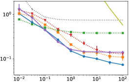
(b) Salary

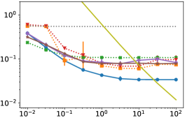
(c) MSNBC

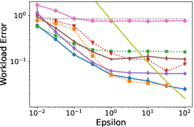
(d) Fire

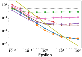
(e) NLTCS

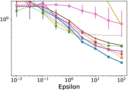
(f) Titanic

Figure 1. Workload error of competing mechanisms on the all-3way workload for $\epsilon=0.01,\dots,100$.

6. Experiments

In this section we empirically evaluate AIM, comparing it to a collection of state-of-the-art mechanisms and baseline mechanisms for a variety of workloads, datasets, and privacy levels.

6.1. Experimental Setup

Datasets

Our evaluation includes datasets with varying size and dimensionality. We describe our exact pre-processing scheme in Appendix A, and summarize the pre-processed datasets and their characteristics in the table below.

Table 2. Summary of datasets used in the experiments.

Dataset	Records	Dimensions	Min/Max	Total
			Domains	Domain Size
adult (Kohavi et al., 1996)	48842	15	2–42	$4\times 10^{16}$
salary (Hay et al., 2016)	135727	9	3–501	$1\times 10^{13}$
msnbc (Cadez et al., 2000)	989818	16	18	$1\times 10^{20}$
fire (Ridgeway et al., 2021)	305119	15	2–46	$4\times 10^{15}$
nltcs (Manton, 2010)	21574	16	2	$7\times 10^{4}$
titanic (Frank E. Harrell Jr., [n.d.])	1304	9	2–91	$9\times 10^{7}$

Workloads

We consider 3 workloads for each dataset, all-3way, target, and skewed. Each workload contains a collection of 3-way marginal queries. The all-3way workload contains queries for all 3-way marginals. The target workload contains queries for all 3-way marginals involving some specified target attribute. For the adult and titanic datasets, these are the income¿50K attribute and the Survived attribute, as those correspond to the attributes we are trying to predict for those datasets. For the other datasets, the target attribute is chosen uniformly at random. The skewed workload contains a collection of 3-way marginal queries biased towards certain attributes and attribute combinations. In particular, each attribute is assigned a weight sampled from a squared exponential distribution. 256 triples of attributes are sampled with probability proportional to the product of their weights. This results in workloads where certain attributes appear far more frequently than others, and is intended to capture the situation where analysts focus on a small number of interesting attributes. All randomness in the construction of the workload was done with a fixed random seed, to ensure that the workloads remain the same across executions of different mechanisms and parameter settings.

Mechanisms

We compare against both workload-agnostic and workload-aware mechanisms in this section. The workload-agnostic mechanisms we consider are PrivBayes+PGM, MST, PrivMRF. The workload-aware mechanisms we consider are MWEM+PGM, RAP, GEM, and AIM. We set the hyper-parameters of every mechanism to default values available in their open source implementations. We also consider baseline mechanisms: Independent and Gaussian. The former measures all 1-way marginals using the Gaussian mechanism, and generates synthetic data using an independence assumption. The latter answers all queries in the workload using the Gaussian mechanism (using the optimal privacy budget allocation described in (Zhang et al., 2021)). Note that this mechanism does not generate synthetic data, only query answers.

Privacy Budgets

We consider a wide range of privacy parameters, varying $\epsilon\in[0.01,100.0]$ and setting $\delta=10^{-9}$. The most practical regime is $\epsilon\in[0.1,10.0]$, but mechanism behavior at the extremes can be enlightening so we include them as well.

Evaluation.

For each dataset, workload, and $\epsilon$, we run each mechanism for 5 trials, and measure the workload error from Definition 2. We report the average workload error across the five trials, along with error bars corresponding to the minimum and maximum workload error observed across the five trials.

Runtime Environment.

We ran most experiments on a single core of a compute cluster with a 4 GB memory limit and a 24 hour time limit. These resources were not sufficient to run PrivMRF or RAP, so we utilized different machines to run those mechanisms. PrivMRF requires a GPU to run, so we used one node a different compute cluster, which has a Nvidia GeForce RTX 2080 Ti GPU. RAP required significant memory resources, so we ran those experiments on a machine with 16 cores and 64 GB of RAM.

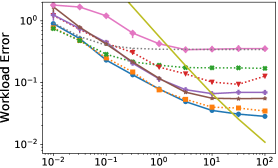
(a) Adult

(b) Salary

(c) MSNBC

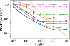
(d) Fire

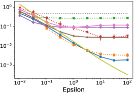
(e) NLTCS

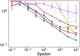
(f) Titanic

Figure 2. Workload error of competing mechanisms on the target workload for $\epsilon=0.01,\dots,100$.

6.2. all-3way Workload

Results on the all-3way workload are shown in Figure 1. Workload-aware mechanisms are shown by solid lines, while workload-agnostic mechanisms are shown with dotted lines. From these plots, we make the following observations:

1. AIM consistently achieves competitive workload error, across all datasets and privacy regimes considered. On average, across all six datasets and nine privacy parameters, AIM improved over PrivMRF by a factor of $1.3\times$, MST by a factor of $8.4\times$, MWEM+PGM by a factor $2.1\times$, PrivBayes+PGM by a factor $2.6\times$, RAP by a factor $9.5\times$, and GEM by a factor $2.3\times$. In the most extreme cases, AIM improved over PrivMRF by a factor $3.6\times$, MST by a factor $118\times$, MWEM+PGM by a factor $16\times$, PrivBayes+PGM by a factor $14.7\times$, RAP by a factor $47.1\times$, and GEM by a factor $11.7\times$.

2. Prior to AIM, PrivMRF was consistently the best performing mechanism, even outperforming all workload-aware mechanisms. The all-3way workload is one we expect workload agnostic mechanisms like PrivMRF to perform well on, so it is interesting, but not surprising that it outperforms workload-aware mechanisms in this setting.

3. Prior to AIM, the best workload-aware mechanism varied for different datasets and privacy levels: MWEM+PGM was best in 65% of settings, GEM was best in 35% of settings , and RAP was best in 0% of settings. Including AIM, we observe that it is best in 85% of settings, followed by MWEM+PGM in 11% of settings and GEM in 4% of settings. Additionally, in the most interesting regime for practical deployment $(\epsilon\geq 1.0)$, AIM is best in 100% of settings.

6.3. target Workload

Results for the target workload are shown in Figure 2. For this workload, we expect workload-aware mechanisms to have a significant advantage over workload-agnostic mechanisms, since they are aware that marginals involving the target are inherently more important for this workload. From these plots, we make the following observations:

1. All three high-level findings from the previous section are supported by these figures as well.

2. Somewhat surprisingly, PrivMRF outperforms all workload-aware mechanisms prior to AIM on this workload. This is an impressive accomplishment for PrivMRF, and clearly highlights the suboptimality of existing workload-aware mechanisms like MWEM+PGM, GEM, and RAP. Even though PrivMRF is not workload-aware, it is clear from their paper that every detail of the mechanism was carefully thought out to make the mechanism work well in practice, which explains it’s impressive performance. While AIM did outperform PrivMRF again, the relative performance did not increase by a meaningful margin — offering a $1.4\times$ improvement on average and a $4.6\times$ improvement in the best case.

6.4. skewed Workload

Results for the skewed workload are shown in Figure 3. For this workload, we again expect workload-aware mechanisms to have a significant advantage over workload-agnostic mechanisms, since they are aware of the exact (biased) set of marginals used to judge utility. From these plots, we make the following observations:

1. All four high-level findings from the previous sections are generally supported by these figures as well, with the following interesting exception:

2. PrivMRF did not score well on salary, and while it was still generally the second best mechanism on the other datasets (again out-performing the workload-aware mechanisms in many cases), the improvement offered by AIM over PrivMRF is much larger for this workload, averaging a $2\times$ improvement with up to a $5.7\times$ improvement in the best case. We suspect for this setting, workload-awareness is essential to achieve strong performance.

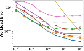
(a) Adult

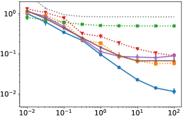
(b) Salary

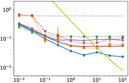
(c) MSNBC

(d) Fire

(e) NLTCS

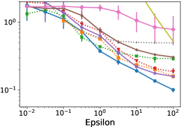
(f) Titanic

Figure 3. Workload error of competing mechanisms on the skewed workload for $\epsilon=0.01,\dots,100$.

6.5. Tuning Model Capacity

In Line 12 of AIM (Algorithm 4), we construct a set of candidates to consider in the current round based on an upper limit on JT-SIZE. 80 MB was chosen to match prior work, but in general we can tune it as desired to strike the right accuracy / runtime trade-off. Unlike other hyper-parameters, there is no “sweet spot” for this one: setting larger model capacities should always make the mechanism perform better, at the cost of increased runtime. We demonstrate this trade-off empirically in Figure 4 (a-b). For $\epsilon=0.1,1,$ and $10$, we considered model capacities ranging from 1.25 MB to 1.28 GB, and ran AIM on the fire dataset with the all-3way workload. Results are averaged over five trials, with error bars indicating the min/max runtime and workload error across those trials. Our main findings are listed below:

1. As expected, runtime increases with model capacity, and workload error decreases with capacity. The case $\epsilon=0.1$ is an exception, where both the plots level off beyond a capacity of $20MB$. This is because the capacity constraint is not active in this regime: AIM already favors small marginals when the available privacy budget is small by virtue of the quality score function for marginal query selection, so the model remains small even without the model capacity constraint.

2. Using the default model capacity and $\epsilon=1$ resulted in a 9 hour runtime. We can slightly reduce error further, by about $13\%$, by increasing the model capacity to $1.28GB$ and waiting 7 days. Conversely, we can reduce the model capacity to $5MB$ which increases error by about $75\%$, but takes less than one hour. The law of diminishing returns is at play.

Ultimately, the model capacity to use is a policy decision. In real-world deployments, it is certainly reasonable to spend additional computational time for even a small boost in utility.

6.6. Uncertainty Quantification

In this section, we demonstrate that our expressions for uncertainty quantification correctly bound the error, and evaluate how tight the bound is. For this experiment, we ran AIM on the fire dataset with the all-3way workload at $\epsilon=10$. In Figure 4 (c), we plot the true error of AIM on each marginal in the workload against the error bound predicted by our expressions. We set $\lambda=1.7$ in Corollary 3, and $\lambda_{1}=2.7$, $\lambda_{2}=3.7$ in Corollary 5, which provides 95% confidence bounds. Our main findings are listed below:

1. For all marginals in the (downward closure of the) workload, the error bound is always greater than true error. This confirms the validity of the bound, and suggests they are safe to use in practice. Note that even if some errors were above the bounds, that would not be inconsistent with our guarantee, as at a 95% confidence level, the bound could fail to hold 5% of the time. The fact that it doesn’t suggests there is some looseness in the bound.

2. The true errors and the error bounds vary considerably, ranging from $10^{-4}$ all the way up to and beyond $1$. In general, the supported marginals have both lower errors, and lower error bounds than the unsupported marginals, which is not surprising. The error bounds are also tighter for the supported marginals. The median ratio between error bound and observed error is $4.4$ for supported marginals and $8.3$ for unsupported marginals. Intuitively, this makes sense because we know selected marginals should have higher error than non-selected marginals, but the error of the non-selected marginal can be far below that of the selected marginal (and hence the bound), which explains the larger gap between the actual error and our predicted bound.

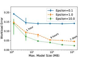
(a) Workload Error vs. Model Capacity

(b) Runtime vs. Model Capacity

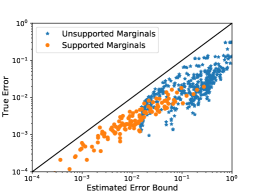
(c) True Error vs. Error Bound

Figure 4.

7. Limitations and Open Problems

In this work, we have carefully studied the problem of workload-aware synthetic data generation under differential privacy, and proposed a new mechanism for this task. Our work significantly improves over prior work, although the problem remains far from solved, and there are a number of promising avenues for future work in this space. We enumerate some of the limitations of AIM below, and identify potential future research directions.

Handling More General Workloads

In this work, we restricted our attention to the special-but-common case of weighted marginal query workloads. Even in this special case, there are many facets to the problem and nuances to our solution. Designing mechanisms that work for the more general class of linear queries (perhaps defined over the low-dimensional marginals) remains an important open problem. While the prior work, MWEM+PGM, RAP, and GEM can handle workloads of this form, they achieve this by selecting a single counting query in each round, rather than a full marginal query, and thus there is likely significant room for improvement. Beyond linear query workloads, other workloads of interest include more abstract objectives like machine learning efficacy and other non-linear query workloads. These metrics have been used to evaluate the quality of workload-agnostic synthetic data mechanisms, but have not been provided as input to the mechanisms themselves. In principle, if we know we want to run a given machine learning model on the synthetic dataset, we should be able to tailor the synthetic data to provide high utility on that model.

Handling Mixed Data Types

In this work, we assumed the input data was discrete, and each attribute had a finite domain with a reasonably small number of possible values. Data with numerical attributes must be appropriately discretized before running AIM. The quality of the discretization could have a significant impact on the quality of the generated synthetic data. Designing mechanisms that appropriately handle mixed (categorical and numerical) data type is an important problem. There may be more to this problem than meets the eye: a new definition of a workload and utility metric may be in order, and new types of measurements and post-processing techniques may be necessary to handle numerical data. Note that some mechanisms, like GAN-based mechanisms, expect numerical data as input, and categorical data must be one-hot encoded prior to usage. While they do handle handle numerical data, their utility is often not competitive with even the simplest marginal-based mechanisms we considered in this work (Tao et al., 2021).

Utilizing Public Data

A promising avenue for future research is to design synthetic data mechanisms that incorporate public data in a principled way. There are many places in which public data can be naturally incorporated into AIM, and exploring these ideas is a promising way to boost the utility of AIM in real world settings where public data is available. Early work on this problem includes (Liu et al., 2021b; McKenna et al., 2021a; Liu et al., 2021a), but these solutions leave room for improvement.

8. Related Work

In Section 3 we focused our discussion on marginal-based mechanisms in the select-measure-generate paradigm. While this is a popular approach, it is not the only way to generate differentially private synthetic data. In this section we provide a brief discussion of other methods, and a broad overview of other relevant work.

One prominent approach is based on differentially private GANs. Several architectures and private learning procedures have been proposed under this paradigm (Jordon et al., 2019; Zhang et al., 2018; Tantipongpipat et al., 2019; Frigerio et al., 2019; Xie et al., 2018; Beaulieu-Jones et al., 2019; Abay et al., 2018; Torfi et al., 2022; Torkzadehmahani et al., 2019). Despite their popularity, we are not aware of evidence that these GAN-based mechanisms outperform even baseline marginal-based mechanisms like PrivBayes on structured tabular data. Most empirical evaluations of GAN-based mechanisms exclude PrivBayes, and the comparisons that we are aware of show the opposite effect: that marginal-based mechanisms outperform the competition (Cai et al., 2021; Tao et al., 2021; McKenna et al., 2021a). GAN-based methods may be better suited for different data modalities, like image or text data.

One exception is CT-GAN (Xu et al., 2019), which is an algorithm for synthetic data that does compare against PrivBayes and does outperform it in roughly 85% of the datasets and metrics they considered. However, this method does not satisfy or claim to satisfy differential privacy, and gives no formal privacy guarantee to the individuals who contribute data. Nevertheless, an empirical comparison between CT-GAN and newer methods for synthetic data, like AIM and PrivMRF, would be interesting, since these mechanisms also outperformed PrivBayes+PGM in nearly every tested situation, and PrivBayes+PGM outperforms PrivBayes most of the time as well (McKenna et al., 2019; Cai et al., 2021). Differentially private implementations of CT-GAN have been proposed, but empirical evaluations of the method suggest it is not competitive with PrivBayes (Rosenblatt et al., 2020; Tao et al., 2021).

Appendix A Data Preprocessing

We apply consistent preprocessing to all datasets in our empirical evaluation. There are three steps to our preprocessing procedure, described below:

Attribute selection

For each dataset, we identify a set of attributes to keep. For the adult, salary, nltcs, and titanic datasets, we keep all attributes from the original data source. For the fire dataset, we drop the 15 attributes relating to incident times, since after discretization, they contain redundant information. The msnbc dataset is a streaming dataset, where each row has a different number of entries. We keep only the first 16 entries for each row.

Domain identification

Usually we expect the domain to be supplied separately from the data file. For example, the IPUMS website contains comprehensive documentation about U.S. Census data products. However, for the datasets we used, no such domain file was available. Thus, we “cheat” and look at the active domain to automatically derive a domain file from the dataset. For each attribute, we identify if it is categorical or numerical. For each categorical attribute, we list the set of observed values (including null) for that attribute, which we treat as the set of possible values for that attribute. For each numerical attribute, we record the minimum and maximum observed value for that attribute.

Discretization

We discretize each numerical attribute into $32$ equal-width bins, using the min/max values from the domain file. This turns each numerical attribute into a categorical attribute, satisfying our assumption.

Appendix B Uncertainty Quantification Proofs

B.1. The Easy Case: Supported Marginals

See 1

Proof.

For each $r_{i}\supseteq r$, we observe $\tilde{y}_{i}\sim M_{r_{i}}(D)+\mathcal{N}(0,\sigma_{i}^{2}\mathbb{I})$. We can use this noisy marginal to obtain an unbiased estimate $M_{r}(D)$ by marginalizing out attributes in the set $r_{i}\setminus r$. This requires summing up $n_{r_{i}}/n_{r}$ cells, so the variance in each cell becomes $n_{r_{i}}\sigma_{i}^{2}/n_{r}$. Moreover, the noise is still normally distributed, since the sum of independent normal random variables is normal. We thus have such an estimate for each $i$ satisfying $r_{i}\supseteq r$, and we can combine these independent estimates using inverse variance weighting (Hartung et al., 2008), resulting in an unbiased estimator with the stated variance. For the same reason as before, the noise is still normally distributed. ∎

See 2

Proof.

Noting that $M_{r}(D)-\bar{y}\sim\mathcal{N}(0,\sigma^{2}\mathbb{I})$, the statement is a direct consequence of Theorem 1, below. ∎

Theorem 1.

Let $x\sim N(0,\sigma^{2})^{n}$, then:

$$\mathbb{E}[\left\lVert x\right\rVert_{1}]=\sqrt{2/\pi}n\sigma$$

and

$$\Pr[\left\lVert x\right\rVert_{1}\geq\sqrt{2\log{2}}\sigma n+c\sigma\sqrt{2n}]\leq\exp{(-c^{2})}$$

Proof.

First observe that $|x_{i}|$ is a sample from a half-normal distribution. Thus, $\mathbb{E}[x_{i}]=\sqrt{2/\pi}\sigma$. From the linearity of expectation, we obtain $\mathbb{E}[\left\lVert x\right\rVert_{1}]=\sqrt{2/\pi}\sigma n$, as desired. For the second statement, we begin by deriving the moment generating function of the random variable $|x_{i}|$. By definition, we have:

$$\mathbb{E}[\exp{(t\cdot|x_{i}|)}] =\int_{-\infty}^{\infty}\phi(z)\exp{(t\cdot|z|)}dz$$

$$=2\int_{0}^{\infty}\phi(z)\exp{(t\cdot z)}dz$$

$$=2\int_{0}^{\infty}\frac{1}{\sigma\sqrt{2\pi}}\exp{\Big{(}-\frac{z^{2}}{2\sigma^{2}}\Big{)}}\exp{(t\cdot z)}dz$$

$$=\frac{1}{\sigma}\sqrt{\frac{2}{\pi}}\int_{0}^{\infty}\exp{\Big{(}-\frac{z^{2}}{2\sigma^{2}}+t\cdot z\Big{)}}dz$$

$$=\exp{\Big{(}\frac{\sigma^{2}t^{2}}{2}\Big{)}}\Big{(}\Phi\Big{(}\frac{t\sigma}{\sqrt{2}}\Big{)}+1\Big{)}$$

Moreover, since $\left\lVert x\right\rVert_{1}=\sum_{i=1}^{n}|x_{i}|$ is a sum of i.i.d random variables, the moment generating function of $\left\lVert x\right\rVert_{1}$ is:

$$\mathbb{E}[\exp{(t\cdot\left\lVert x\right\rVert_{1})}]=\exp{\Big{(}\frac{\sigma^{2}t^{2}}{2}\Big{)}}^{n}\Big{(}\Phi\Big{(}\frac{t\sigma}{\sqrt{2}}\Big{)}+1\Big{)}^{n}$$

From the Chernoff bound, we have

$$\Pr[\left\lVert x\right\rVert_{1}\geq a] \leq\min_{t\geq 0}\frac{\mathbb{E}[\exp{(t\cdot\left\lVert x\right\rVert_{1})}]}{\exp{(ta)}}$$

$$=\min_{t\geq 0}\exp{\Big{(}\frac{n\sigma^{2}t^{2}}{2}-ta\Big{)}}\Big{(}\Phi\Big{(}\frac{t\sigma}{\sqrt{2}}\Big{)}+1\Big{)}^{n}$$

$$\leq\min_{t\geq 0}2^{n}\exp{\Big{(}\frac{n\sigma^{2}t^{2}}{2}-ta\Big{)}}$$

$$\leq 2^{n}\exp{\Big{(}\frac{n\sigma^{2}(a/n\sigma^{2})^{2}}{2}-(a/n\sigma^{2})a}\Big{)}$$

$$=2^{n}\exp{\Big{(}\frac{a^{2}}{2n\sigma^{2}}-\frac{a^{2}}{n\sigma^{2}}\Big{)}}$$

$$=2^{n}\exp{\Big{(}-\frac{a^{2}}{2n\sigma^{2}}\Big{)}}$$

$$=\exp{\Big{(}-\frac{a^{2}}{2n\sigma^{2}}+n\log{2}\Big{)}}$$

With some further manipulation of the bound, we obtain:

($$a=d\sigma\sqrt{2n} \Pr[\left\lVert x\right\rVert_{1}\geq d\sigma\sqrt{2n}]\leq\exp{\Big{(}-d^{2}+n\log{2}\Big{)}}$$)

($$d=c+\sqrt{n\log{2}} \Pr[\left\lVert x\right\rVert_{1}\geq(c+\sqrt{n\log{2}})\sigma\sqrt{2n}]\leq\exp{(-c^{2})}$$)

$$\Pr[\left\lVert x\right\rVert_{1}\geq\sqrt{2\log{2}}\sigma n+c\sigma\sqrt{2n}]\leq\exp{(-c^{2})}$$

∎

B.2. The Hard Case: Unsupported Marginals

See 4

Proof.

By the guarantees of the exponential mechanism, we know that, with probability at most $e^{-\lambda_{2}}$, for all $r\in C_{t}$ we have:

$$q_{r_{t}}\leq q_{r}-\frac{2\Delta_{t}}{\epsilon_{t}}(\log{(|C_{t}|)}+\lambda_{2})$$

Now define $E_{r}=\left\lVert M_{r}(D)-M_{r}(p_{t-1})\right\rVert_{1}$. Plugging in $q_{r}=w_{r}(E_{r}-\sqrt{2/\pi}\sigma_{t}n_{r})$ and rearranging gives:

$$E_{r}\geq\frac{w_{r_{t}}(E_{r_{t}}-\sqrt{2/\pi}\sigma_{t}n_{r_{t}})+\frac{2\Delta_{t}}{\epsilon_{t}}(\log{(|C_{t}|)+\lambda_{2})}}{w_{r}}+\sqrt{2/\pi}\sigma_{t}n_{r}$$

From Theorem 2, with probability at most $e^{-\lambda_{1}^{2}/2}$, we have:

$$\left\lVert M_{r_{t}}(p_{t-1})-y_{t}\right\rVert_{1}+\lambda_{1}\sigma_{t}\sqrt{n_{r_{t}}}\leq E_{r_{t}}$$

Combining these two facts via the union bound, along with some algebraic manipulation, yields the stated result. ∎

Theorem 2.

Let $a,b\in\mathbb{R}^{k}$ and let $c=b+z$ where $z\sim\mathcal{N}(0,\sigma^{2})^{n}$.

$$\Pr[\left\lVert a-c\right\rVert_{1}\leq\left\lVert a-b\right\rVert_{1}-\lambda\sigma\sqrt{n}]\leq\exp{\Big{(}-\frac{1}{2}\lambda^{2}\Big{)}}$$

Proof.

First note that $|a_{i}-c_{i}|=|a_{i}-b_{i}-z_{i}|$, which is distributed according to a folded normal distribution with mean $|a_{i}-b_{i}|$. It is well known (Tsagris et al., 2014) that the moment generating function for this random variable is $M_{i}(t)$, where:

$$M_{i}(t) =\exp{\Big{(}\frac{1}{2}\sigma^{2}t^{2}+|a_{i}-b_{i}|t\Big{)}}\Phi(|a_{i}-b_{i}|/\sigma+\sigma t)$$

$$+\exp{\Big{(}\frac{1}{2}\sigma^{2}t^{2}-|a_{i}-b_{i}|t\Big{)}}\Phi(-|a_{i}-b_{i}|/\sigma+\sigma t).$$

Moreover, the moment generating function of $\left\lVert a-c\right\rVert_{1}$ is $M(t)=\prod_{i}M_{i}(t)$. We will begin by focusing our attention on bounding $M_{i}(-t)$. For simplicity, let $\mu=|a_{i}-b_{i}|$. We have:

$$M_{i}(-t)= \exp{\Big{(}\frac{\sigma^{2}t^{2}}{2}-\mu t\Big{)}}\Phi(\mu/\sigma-\sigma t)$$

$$+\exp{\Big{(}\frac{\sigma^{2}t^{2}}{2}+\mu t\Big{)}}\Phi(-\mu/\sigma-\sigma t)$$

$$= \exp{\Big{(}\frac{\sigma^{2}t^{2}}{2}-\mu t\Big{)}}(1-\Phi(-\mu/\sigma+\sigma t))$$

$$+\exp{\Big{(}\frac{\sigma^{2}t^{2}}{2}+\mu t\Big{)}}\Phi(-\mu/\sigma-\sigma t)$$

$$= \exp{\Big{(}\frac{\sigma^{2}t^{2}}{2}-\mu t\Big{)}}$$

$$-\exp{\Big{(}\frac{\sigma^{2}t^{2}}{2}-\mu t\Big{)}}\Phi(-\mu/\sigma+\sigma t)$$

$$+\exp{\Big{(}\frac{\sigma^{2}t^{2}}{2}+\mu t\Big{)}}\Phi(-\mu/\sigma-\sigma t)$$

(Lemma 3 below; $$a=\sigma t,b=\mu/\sigma \leq \exp{\Big{(}\frac{\sigma^{2}t^{2}}{2}-\mu t\Big{)}}$$)

We are now ready to plug this result into the Chernoff bound, which states:

$$\Pr[\left\lVert a-c\right\rVert_{1}\leq r] \leq\min_{t\geq 0}\exp{(t\cdot r)}M(-t)$$

$$\leq\min_{t\geq 0}\exp{(t\cdot r)}\prod_{i}\exp{\Big{(}\frac{\sigma^{2}t^{2}}{2}-|a_{i}-b_{i}|t\Big{)}}$$

$$=\min_{t\geq 0}\exp{(t\cdot r+\frac{n\sigma^{2}t^{2}}{2}-\left\lVert a-b\right\rVert_{1}t)}$$

Setting $r=\left\lVert a-b\right\rVert_{1}-\lambda\sigma\sqrt{n}$ gives the desired result

$$\Pr [\left\lVert a-c\right\rVert_{1}\leq\left\lVert a-b\right\rVert_{1}-\lambda\sigma\sqrt{n}]$$

$$\leq\min_{t\geq 0}\exp{(t\cdot(\left\lVert a-b\right\rVert_{1}-\lambda\sigma\sqrt{n})+\frac{n\sigma^{2}t^{2}}{2}-\left\lVert a-b\right\rVert_{1}t)}$$

$$=\min_{t\geq 0}\exp{\Big{(}-t\lambda\sigma\sqrt{n}+\frac{n\sigma^{2}t^{2}}{2}\Big{)}}$$

(set $$t=\lambda/\sigma\sqrt{n} \leq\exp{(-\lambda^{2}/2)}$$)

∎

Lemma 0.

Let $a,b\geq 0$, and let $\Phi$ denote the CDF of the standard normal distribution. Then,

$$\exp{\Big{(}\frac{1}{2}a^{2}+ab\Big{)}}\Phi(-a-b)\leq\exp{\Big{(}\frac{1}{2}a^{2}-ab\Big{)}}\Phi(a-b)$$

Proof.

First observe that:

$$\exp{\Big{(}\frac{1}{2}a^{2}+ab\Big{)}}\Phi(-a-b) =\exp{\Big{(}-\frac{1}{2}b^{2}\Big{)}}\frac{\Phi(-a-b)}{\phi(-a-b)}$$

$$\exp{\Big{(}\frac{1}{2}a^{2}-ab\Big{)}}\Phi(a-b) =\exp{\Big{(}-\frac{1}{2}b^{2}\Big{)}}\frac{\Phi(a-b)}{\phi(a-b)}$$

Since $a,b\geq 0$, we know that $-a-b\leq a-b$. We will now argue that the function $\frac{\Phi(\alpha)}{\phi(\alpha)}$ is monotonically increasing in $\alpha$, which suffices to prove the desired claim. To prove this, we will observe that this is this quantity is known as the Mills ratio (Greene, 2003) for the normal distribution. We know that the Mills ratio is connected to a particular expectation; specifically, if $X\sim\mathcal{N}(0,1)$, then

$$\mathbb{E}[X\mid X<\alpha]=-\frac{\phi(\alpha)}{\Phi(\alpha)}$$

Using this interpretation, it is clear that the LHS (and hence the RHS) is monotonically increasing in $\alpha$. Since $-\frac{\phi(\alpha)}{\Phi(\alpha)}$ is monotonically increasing, so is $\frac{\Phi(\alpha)}{\phi(\alpha)}$. ∎

Appendix C Interpretable Error Rate and Subsampling Mechanism

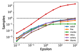
(a) General

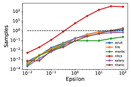
(b) Target

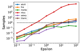
(c) Weighted

Figure 5. Performance of AIM as measured by the number of samples needed to match the achieved workload error.

In Section 6, we saw that AIM offers the best error relative to existing synthetic data mechanisms, although it is not obvious whether a given $L_{1}$ error should be considered “good”. This is necessary for setting the privacy parameters to strike the right privacy/utility tradeoff. We can bring more clarity to this problem by comparing AIM to a (non-private) baseline that simply resamples $K$ records from the dataset. Then, if AIM achieves the same error as resampling $K=\frac{N}{2}$ records, this provides a clear interpretation: that the price of privacy is losing about half the data. Due to the simplicity of this baseline, we can compute the expected workload error in closed form, without actually running the mechanism. We provide details of these calculations in the next section.

Figure 5 plots the performance of AIM on each dataset, epsilon, and workload considered, measured using the fraction of samples needed for the subsampling mechanism to match the performance of AIM. These plots reveal that at $\epsilon=10$, the median subsampling fraction is about $0.37$ for the general workload, $0.62$ for the target workload, and $0.85$ for the weighted workload. At $\epsilon=1$, these numbers are $0.13$, $0.15$, and $0.21$, respectively. The results are comparable across five out of six datasets, with nltcs being a clear outlier. For that dataset, a subsampling fraction of 1.0 was reached by $\epsilon=0.31$ for all workload. This could be an indication of overfitting to the data; a possible reason for this behavior is that the domain size of the nltcs data is small compared to the number of records. mnsbc is also an outlier to a lesser extent, with worse performance than the other datasets for larger $\epsilon$. A possible reason for this behavior is that msnbc has the most data points, so subsampling with the same fraction of points has much lower error. AIM may not be able to match that low error due to the computational constraints imposed on the model size, combined with the fact that this dataset has a large domain.

C.1. Mathematical Details of Subsampling

We begin by analyzing the expected workload error of the (non-private) mechanism that randomly samples $K$ items with replacement from $D$. Then, we will connect that to the error of AIM, and determine the value of $K$ where the error rates match. Theorem 1 gives a closed form expression for the expected $L_{1}$ error on a single marginal as a function of the number of sampled records.

Theorem 1.

Let $\hat{D}$ be the dataset obtained by sampling $K$ items with replacement from $D$. Further, let $\vec{\mu}=\frac{1}{N}M_{r}(D)$ and $\vec{s}=\lceil K\vec{\mu}\rceil$.

$$\mathbb{E} \Big{[}\left\lVert\frac{1}{N}M_{r}(D)-\frac{1}{K}M_{r}(\hat{D})\right\rVert\Big{]}=$$

$$\frac{2}{K}\sum_{x\in\Omega_{r}}s(x)\binom{K}{s(x)}\mu(x)^{s(x)}(1-\mu(x))^{K-s(x)+1}$$

Proof.

The theorem statement follows directly from Lemma 4 and Lemma 3. ∎

Lemma 0 (Mean Deviation (Frame, 1945; Johnson et al., 2005)).

Let $k\sim Binomial(n,p)$, then:

$$\mathbb{E}\Big{[}\Big{|}p-\frac{k}{n}\Big{|}\Big{]}=\frac{2}{n}s\binom{n}{s}p^{s}(1-p)^{n-s+1},$$

where $s=\lceil n\cdot p\rceil$.

Proof.

This statement appears and is proved in (Frame, 1945; Johnson et al., 2005). ∎

Lemma 0 ($L_{1}$ Deviation).

Let $\vec{k}\sim Multinomial(n,\vec{p})$, then:

$$\mathbb{E}[\left\lVert\vec{p}-\vec{k}/n\right\rVert_{1}]=\frac{2}{n}\sum_{x}s(x)\binom{n}{s(x)}p(x)^{s(x)}(1-p(x))^{n-s(x)+1},$$

where $s(x)=\lceil n\cdot p(x)\rceil$.

Proof.

The statement follows immediately from Lemma 2 and the fact that $k(x)\sim Binomial(n,p(x))$. ∎

Lemma 0.

Let $\hat{D}$ be the dataset obtained by sampling $K$ items with replacement from $D$. Then,

$$M_{r}(\hat{D})\sim Multinomial\Big{(}K,\frac{1}{N}M_{r}(D)\Big{)}$$

Proof.

The statement follows from the definition of the multinomial distribution. ∎

Appendix D Structural Zeros

In this section, we describe a simple and principled method to specify and enforce structural zeros in the mechanism. These capture attribute combinations that cannot occur in the real data. Without specifying this, synthetic data mechanisms will usually generate records that violate these constraints that hold in the real data, as the process of adding noise can introduce spurious records, especially in high privacy regimes. These spurious records can be confusing for downstream analysis of the synthetic data, and can lead the analyst to distrust the quality of the data. By imposing known structural zero constraints, we can avoid this problem, while also improving the quality of the synthetic data on the workload of interest.

Structural zeros, if they exist, can usually be enumerated by a domain expert. We can very naturally incorporate these into our mechanism with only one minor change to the underlying Private-PGM library. These structural zeros can be specified as input as a list of pairs $(r,\mathcal{Z}_{r})$ where $\mathcal{Z}_{r}\subseteq\Omega_{r}$. The first entry of the pair specifies the set of attributes relevant to the structural zeros, while the second entry enumerates the attribute combinations whose counts should all be zero. The method we propose can be used within any mechanism that builds on top of Private-PGM, and is hence more broadly useful outside the context of AIM.

To understand the technical ideas in this section, please refer to the background on Private-PGM (McKenna et al., 2019). Usually Private-PGM is initialized by setting $\theta_{r}(x_{r})=0$ for all $r$ in the model and all $x_{r}\in\Omega_{r}$. This corresponds to a model where $\mu_{r}(x_{r})$ is uniform across all $x_{r}$. Our basic observation is that by initializing Private-PGM by setting $\theta_{r}(x_{r})=-\infty$ for each $x_{r}\in Z_{r}$, the cell of the associated marginal will be $\mu_{r}(x_{r})=0$, as desired. Moreover, each update within the Private-PGM estimation procedure will try to update $\theta_{r}(x_{r})$ by a finite amount, leaving it unchanged. Thus, $\mu_{r}(x_{r})$ will remain $0$ during the entire estimation procedure. We conjecture that the estimation procedure solves the following modified convex optimization problem:

$$\hat{\mu}=\min_{\begin{subarray}{c}\mu\in\mathcal{M}\\ \mu_{r}(Z_{r})=0\end{subarray}}L(\mu)$$

This approach is appealing because other simple approaches that discard invalid tuples can inadvertently bias the distribution, which is undesirable.

Note that for each clique in the set of structural zeros, we must include that clique in our model, which increases the size of that model. Thus, we should treat it as we would treat a clique selected by AIM. That is, when calculating JT-SIZE in line 12 of AIM, we need to include both the cliques selected in earlier iterations, as well as the cliques included in the structural zeros.

D.1. Experiments

In this section, we empirically evaluate this structural zeros enhancement, showing that it can reduce workload error in some cases. For this experiment, we consider the general workload on the fire dataset, and compare the performance of AIM with and without imposing structural zero constraints. This dataset contains several related attributes, like “Zipcode of Incident“ and “City”. While these attributes are not perfectly correlated, significant numbers of attribute combinations are impossible. We identified a total of nine attribute pairs which contain some structural zeros, and a total of 2696 structural zero constraints within these nine marginals.

The results of this experiment are shown in Table 3. On average, imposing structural zeros improves the performance of the mechanism, although the improvement is not universal across all values of epsilon we tested. Nevertheless, it is still useful to impose these constraints for data quality purposes.

Table 3. Error of AIM on the fire dataset, with and
without imposing structural zero constraints.

$\epsilon$	AIM	AIM+Structural Zeros	Ratio
0.010	0.613	0.542	1.130
0.031	0.303	0.263	1.151
0.100	0.141	0.153	0.924
0.316	0.087	0.077	1.124
1.000	0.052	0.053	0.979
3.162	0.044	0.045	0.964
10.00	0.038	0.032	1.170
31.62	0.029	0.026	1.149
100.0	0.025	0.025	1.004

Appendix E Runtime Experiments

Our primary focus in the main body of the paper was mechanism utility, as measured by the workload error. In this section we discuss the runtime of AIM, which is an important consideration when deploying it in practice. Note that we do not compare against runtime of other mechanisms here, because different mechanisms were executed in different runtime environments. Figure 6 below shows the runtime of AIM as a function of the privacy parameter. As evident from the figure, runtime increases drastically with the privacy parameter. This is not surprising because AIM is budget-aware: it knows to select larger marginals and run for more rounds when the budget is higher, which in turn leads to longer runtime. For large $\epsilon$, the constraint on JT-SIZE is essential to allow the mechanism to terminate at all. Without it, AIM may try to select marginal queries that exceed memory resources and result in much longer runtime. For small $\epsilon$, this constraint is not active, and could be removed without affecting the behavior of AIM.

Recall that these experiments were conducted on one core of a compute cluster with 4 GB of memory and a CPU speed of 2.4 GHz. These machines were used due to the large number of experiments we needed to conduct, but in real-world scenarios we only need to run one execution of AIM, for a single dataset, workload, privacy parameter, and trial. For this, we can use machines with much better specs, which would improve the runtime significantly.

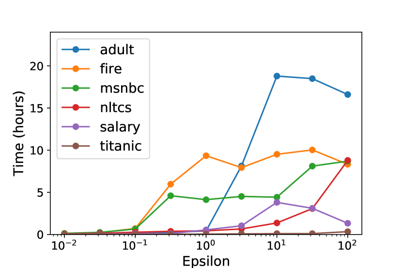
Figure 6. Runtime of AIM on the all-3way workload.

Appendix F Private-PGM vs. Relaxed Projection

(a) $\epsilon=0.1$

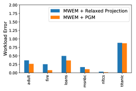
(b) $\epsilon=1.0$

(c) $\epsilon=10.0$

Figure 7. MWEM+Relaxed Projection vs. MWEM+PGM on the all-3way workload.

In this paper, we built AIM on top of Private-PGM, leveraging prior work for the generate step of the select-measure-generate paradigm. Private-PGM is not the only method in this space, although it was the first general purpose and scalable method to our knowledge. “Relaxed Projection” (Aydore et al., 2021) is another general purpose and scalable method that solves the same problem, and could be used in place of Private-PGM if desired. RAP, the main mechanism that utilizes this technique, did not perform well in our experiments. However, it is not clear from our experiments if the poor performance can be attributed to the relaxed projection algorithm, or some other algorithmic design decisions. In this section, we attempt to precisely pin down the differences between these two related methods, taking care to fix possible confounding factors. We thus consider two mechanisms: MWEM+PGM, which is defined in Algorithm 1, and MWEM+Relaxed Projection which is identical to MWEM+PGM in every way, except the call to Private-PGM is replaced with a call to the relaxed projection algorithm of Aydore et al.

For this experiment, we consider the all-3way workload, and we run each algorithm for $T=5,10,\dots,100$, with five trials for each hyper-parameter setting. We average the workload error across the five trials, and report the minimum workload error across hyper-parameter settings in Figure 7. Although the algorithms are conceptually very similar, MWEM+PGM consistently outperforms MWEM+Relaxed Projection, across every dataset and privacy level considered. The performance difference is modest in many cases, but significant on the fire dataset.

AP-PGM (McKenna et al., 2021b) offers another alternative to Private-PGM for the generate step, and while it was shown to be an appealing alternative to Private-PGM in some cases, within the context of an MWEM-style algorithm, their own experiments demonstrate the superiority of Private-PGM.

Generator networks (Liu et al., 2021a) offer yet another alternative to Private-PGM for the generate step. To the best of our knowledge, no direct comparison between this approach and Private-PGM has been done to date, where confounding factors are controlled for. Conceptually, this approach is most similar to the relaxed projection approach, so we conjecture the results to look similar to those shown in Figure 7.