Reduced Higher Order SVD: ubiquitous rank-reduction
method in tensor-based scientific computing

Abstract

Tensor numerical methods, based on the rank-structured tensor representation of $d$-variate functions and operators discretized on large $n^{\otimes d}$ grids, are designed to provide $O(dn)$ complexity of numerical calculations contrary to $O(n^{d})$ scaling by conventional grid-based methods. However, multiple tensor operations may lead to enormous increase in the tensor ranks (curse of ranks) of the target data, making calculation intractable. Therefore one of the most important steps in tensor calculations is the robust and efficient rank reduction procedure which should be performed many times in the course of various tensor transforms in multidimensional operator and function calculus. The rank reduction scheme based on the Reduced Higher Order SVD (RHOSVD) introduced in [33] played a significant role in the development of tensor numerical methods. Here, we briefly survey the essentials of RHOSVD method and then focus on some new theoretical and computational aspects of the RHOSVD demonstrating that this rank reduction technique constitutes the basic ingredient in tensor computations for real-life problems. In particular, the stability analysis of RHOSVD is presented. We recall the performance of the RHOSVD in tensor-based calculation of the Hartree potential in computational quantum chemistry. We introduce the multilinear algebra of tensors represented in the range-separated (RS) tensor format. This allows to apply the RHOSVD rank-reduction techniques to non-regular functional data with many singularities, for example, to the rank-structured computation of the collective multi-particle interaction potentials in bio-molecular modeling, as well as to complicated composite radial functions. The new theoretical and numerical results on application of the RHOSVD in scattered data modeling are presented. We finally underline that RHOSVD proved to be the efficient rank reduction technique in numerous applications ranging from numerical treatment of multi-particle systems in material sciences up to a numerical solution of PDE constrained control problems in $\mathbb{R}^{d}$.

Key words: Reduced higher order SVD, low-rank tensor product approximation, multivariate functions, tensor calculus, rank reduction, Tucker and canonical tensor formats, interaction potentials, scattered data modeling.

AMS Subject Classification: 65F30, 65F50, 65N35, 65F10

1 Introduction

The mathematical models in large-scale scientific computing are often described by steady state or dynamical PDEs. The underlying physical, chemical or biological systems usually live in 3D physical space $\mathbb{R}^{3}$ and may depend on many structural parameters. The solution of arising discrete systems of equation and optimization of the model parameters leads to the challenging numerical problems. Indeed, the accurate grid-based approximation of operators and functions involved requires large spacial grids in $\mathbb{R}^{d}$, leading to the considerable storage space and to the implementation of various algebraic operations on huge vectors and matrices. For further discussion we shall assume that all functional entities are discretized on $n^{\otimes d}$ spacial grids where the univariate grid size $n$ may vary in the range of several thousands. The linear algebra on $N$-vectors and $N\times N$ matrices with $N=n^{d}$ quickly becomes non-tractable as $n$ and $d$ increase.

Tensor numerical methods [59, 60] provide means to overcome the problem of the exponential increase of numerical complexity in the dimension of the problem $d$, due to their intrinsic feature of reducing the computational costs of multilinear algebra on rank-structured data to merely linear scaling in both the grid-size $n$ and dimension $d$. They appeared as bridging of the algebraic tensor decompositions initiated in chemometrics [8, 9, 52, 7, 10, 56, 54] and of the nonlinear approximation theory on separable low-rank representation of multivariate functions and operators [19, 32]. The canonical [23], Tucker [57], tensor train (TT) and hierarchical Tucker (HT) formats [49, 48, 18] are the most commonly used rank-structured parametrizations in applications of modern tensor numerical methods. Further data-compression to the logarithmic scale can be achieved by using the quantized-TT (QTT) [30] tensor approximation. At present there is an active research toward further progress of tensor numerical methods in scientific computing [59, 60, 36, 40, 50]. In particular, there are considerable achievements of tensor-based approaches in computational chemistry [26, 27, 34, 12, 25], in bio-molecular modeling [3, 4, 31, 38], in optimal control problems (including the case of fractional control) [22, 11, 13, 53], and in many other fields [2, 5, 15, 42, 7, 41].

Here we notice that tensor numerical methods proved to be efficient when all input data and all intermediate quantities within the chosen computational scheme are presented in certain low-rank tensor format with controllable rank parameters, i.e. on low-rank tensor manifolds. In turn, tensor decomposition of the full format data arrays is considered as N-P hard problem. For example, the truncated HOSVD [10] of an $n^{\otimes d}$-tensor in the Tucker format amounts to $O(n^{d+1})$ arithmetic operations while the respective cost of the TT and HT higher-order SVD [46, 17] is estimated by $O(n^{\frac{3}{2}d})$, indicating that rank decomposition of full format tensors still suffers from the “curse of dimensionality” and practically could not be applied in large scale computations.

On the other hand, often, the initial data for complicated numerical algorithms may be chosen in the canonical/Tucker tensor formats, say as a result of discretization of a short sum of Gaussians or multivariate polynomials, or as a result of the analytical approximation by using Laplace transform representation and sinc-quadratures [59]. However, the ranks of tensors are multiplied in the course of various tensor operations, leading to dramatical increase in the rank parameter (“curse of ranks”) of a resulting tensor, thus making tensor-structured calculation intractable. Therefore, a stable rank reduction schemes are the main prerequisite for the success of rank-structured tensor techniques.

Invention of the Reduced Higher Order SVD (RHOSVD) in [33] and the corresponding rank reduction procedure based on the canonical-to-Tucker transform and subsequent canonical approximation of the small Tucker core (Tucker-to-canonical transform) was a decisive step in development of the tensor numerical methods in scientific computing. In contrast to the conventional HOSVD, the RHOSVD does not need a construction of the full size tensor for finding the orthogonal subspaces of the Tucker tensor representation. Instead, RHOSVD applies to numerical data in the canonical tensor format (with possibly large initial rank $R$) and exhibits the $O(dnR\min\{n,R\})$ complexity, uniformly in the dimensionality of the problem, $d$, and it was an essential step ahead in development of tensor-structured numerical techniques.

In particular, this rank reduction scheme was applied to calculation of 3D and 6D convolution integrals in tensor-based solution of the Hartree-Fock equation [33, 26]. Combined with the Tucker-to-canonical transform, this algorithm provides a stable procedure for the rank reduction of possibly huge ranks in tensor-structured calculations of the Hartree potential. The RHOSVD based rank reduction scheme for the canonical tensors is specifically useful for 3D problems, which are most often in real-life applications. However, the RHOSVD-like procedure can be also efficiently applied in the construction of the TT tensor format from the canonical tensor input, which often appears in tensor calculations.

The RHOSVD is the basic tool for the construction of the range-separated (RS) tensor format introduced in [3] for the low-rank tensor representation of the bio-molecular long-range electrostatic potentials. Recent example on the RS representation of the multi-centered Dirac delta function [31] paves the way for efficient solution decomposition scheme introduced for the Poisson-Boltzmann equation [4, 38].

In some applications the data could be presented as a sum of highly localized and rank-structured components so that their further numerical treatment again requires the rank reduction procedure (see section 4.5 concerning the long-range potential calculation for many-particle system). Here, we consider the example on representation of the scattered data by a sum of Slater kernels and show the existence of the low-rank representation for such data in the RS tensor format. The numerical examples demonstrate the practical efficiency of such kind of tensor interpolation.

Rank reduction procedure by using the RHOSVD is a mandatory part in solving the three-dimensional elliptic and pseudo-differential equations in the rank-structured tensor format. In the course of preconditioned iterations, the tensor ranks of the governing operator, the precoditioner and of the current iterand are multiplied at each iterative step, and therefore a fast and robust rank reduction techniques is the prerequisite for such methodology applied in the framework of iterative elliptic problem solvers. In particular, this approach was applied to the PDE constrained (including the case of fractional operators) optimal control problems [22, 53]. As result, the computational complexity can be reduced to almost linear scale, $O(nR)$, contrary to conventional $O(n^{3})$ complexity, as demonstrated by numerics in [22, 53].

Tensor-based algorithms and methods are now being widely used and developed further in the communities of scientific computing and data science. Tensor techniques evolve in traditional tensor decompositions in data processing [52, 15, 14], and they are actively promoted for tensor-based solution of the multidimensional problems in numerical analysis and quantum chemistry [34, 50, 53, 59, 34, 37, 13, 47]. Notice that in the case of higher dimensions the rank reduction in the canonical format can be performed directly (i.e., without intermediate use of the Tucker approximation) by using the cascading ALS iteration in the CP format, see [35] concerning the tensor-structured solution of the stochastic/parametric PDEs.

The rest of the papers is organized as follows. In section 2 we sketch some results on the construction of the RHOSVD and present some old and new results on the stability of error bounds. In section 2.2 we discuss the mixed canonical-Tucker tensor format and the Tucker-to-canonical transform. Section 3 recalls the results from [26] on calculation of the multidimensional convolution integrals with the Newton kernel arising in computational quantum chemistry. Section 4 addresses the application of RHOSVD to RS parametrized tensors. In §4.2 we discuss the application of RHOSVD in multilinear operations of data in the RS tensor format. The scattered data modeling is considered in §4.5 from both theoretical and computational aspects. Application of RHOSVD for tensor-based representation of Greens kernels is discussed in section 5. Section 6 gives a short sketch of RHOSVD in application to tensor-structured elliptic problem solvers.

2 Reduced HOSVD and CP-to-Tucker Transform

2.1 Reduced HOSVD: error bounds

In computational schemes including bilinear tensor-tensor or matrix-tensor operations the increase of tensor ranks leads to the critical loss of efficiency. Moreover, in many applications, for example in electronic structure calculations, the canonical tensors with large rank parameters arise as the result of polynomial type or convolution transforms of some function related tensors (say, electron density, the Hartree potential, etc.). In what follows, we present the new look on the direct method of rank reduction for the canonical tensors with large initial rank, the reduced HOSVD, first introduced and analyzed in [33].

We denote by $\mbox{\boldmath{$\mathcal{T}$}}_{{\bf r},{\bf n}}$ the class of tensors ${\bf A}\in\mathbb{R}^{n\otimes d}$ parametrized in the rank-${\bf r}$, ${\bf r}=(r_{1},\cdots,r_{d})$ orthogonal Tucker format,

$${\bf A}={\boldsymbol{\beta}}\times_{1}V^{(1)}\times_{2}\cdots\times_{d}V^{(d)}\in\mbox{\boldmath{$\mathcal{T}$}}_{{\bf r},{\bf n}},$$

with the orthogonal side-matrices $V^{(\ell)}=[{\bf v}^{(\ell)}_{1}\ldots{\bf v}^{(\ell)}_{r_{\ell}}]\in\mathbb{R}^{n\times r_{\ell}}$ and with the core coefficient tensor ${\boldsymbol{\beta}}\in\mathbb{R}^{r_{1}\times...\times r_{d}}$.

Likewise, $\mbox{\boldmath{$\mathcal{C}$}}_{{R},{\bf n}}$ denotes the class of rank-$R$ canonical tensors. For given ${\bf A}\in\mbox{\boldmath{$\mathcal{C}$}}_{{R},{\bf n}}$ in the rank-$R$ canonical format,

$${\bf A}={\sum}_{\nu=1}^{R}\xi_{\nu}{\bf u}^{(1)}_{\nu}\otimes\ldots\otimes{\bf u}^{(d)}_{\nu},\quad\xi_{\nu}\in\mathbb{R},$$ (2.1)

with normalized canonical vectors, i.e. $\|{\bf u}^{(\ell)}_{\nu}\|=1$ for $\ell=1,...,d$, $\nu=1,...,R$.

The standard algorithm for the Tucker tensor decomposition [10] is based on HOSVD applied to full tensors of size $n^{d}$ which exhibits $O(n^{d+1})$ computational complexity. The question is how to simplify the HOSVD Tucker approximation in the case of canonical input tensor in the form (2.1) without use of the full format representation of ${\bf A}$, and in the situation when the CP rank parameter $R$ and the mode sizes $n$ of the input can be sufficiently large.

First, let us use the equivalent (nonorthogonal) rank-${\bf r}=(R,...,R)$ Tucker representation of the tensor (2.1),

$${\bf A}=\boldsymbol{\xi}\times_{1}{U}^{(1)}\times_{2}{U}^{(2)}\cdots\times_{d}{U}^{(d)},\quad\boldsymbol{\xi}=diag\{\xi_{1},...,\xi_{R}\},$$ (2.2)

via contraction of the diagonal tensor $\boldsymbol{\xi}=diag\{\xi_{1},...,\xi_{R}\}\in\mathbb{R}^{R\otimes d}$ with $\ell$-mode side matrices $U^{(\ell)}=[{\bf u}^{(\ell)}_{1},...,{\bf u}^{(\ell)}_{R}]\in\mathbb{R}^{n\times R}$, see Figure 2.1.

Figure 2.1: Contracted product representation of the rank-$R$ canonical tensor.

Then the problem of canonical to Tucker approximation can be solved by the method of reduced HOSVD (RHOSVD) introduced in [33]. The basic idea of the reduced HOSVD is that for large (function related) tensors given in the canonical format their HOSVD does not require the construction of a tensor in the full format and SVD based computation of its matrix unfolding. Instead, it is sufficient to compute the SVD of the directional matrices $U^{(\ell)}$ in (2.2) composed by only the vectors of the canonical tensor in every dimension separately, as shown in Figure 2.1. This will provide the initial guess for the Tucker orthogonal basis in the given dimension. For the practical applicability, the results of the approximation theory on the low-rank approximation to the multivariate functions, exhibiting exponential error decay in the Tucker rank, are of the principal significance [29].

In what follows, we suppose that $n\leq R$ and denote the SVD of the side-matrix $U^{(\ell)}$ by

$$U^{(\ell)}={Z}^{(\ell)}D_{\ell}{V^{(\ell)}}^{T}=\sum\limits_{k=1}^{n}\sigma_{\ell,k}{\bf z}_{k}^{(\ell)}\;{{\bf v}_{k}^{(\ell)}}^{T},\quad{\bf z}_{k}^{(\ell)}\in\mathbb{R}^{n},\;{\bf v}_{k}^{(\ell)}\in\mathbb{R}^{R},$$ (2.3)

with the orthogonal matrices ${Z}^{(\ell)}=[{\bf z}_{1}^{(\ell)},...,{\bf z}_{n}^{(\ell)}]\in\mathbb{R}^{n\times n}$, and ${V}^{(\ell)}=[{\bf v}_{1}^{(\ell)},...,{\bf v}_{n}^{(\ell)}]\in\mathbb{R}^{R\times n}$, $\ell=1,...,d$. We use the following notations for the vector entries, $v_{k}^{(\ell)}(\nu)=v_{k,\nu}^{(\ell)}$ ($\nu=1,...,R$).

To fix the idea, we introduce the vector of rank parameters, ${\bf r}=(r_{1},...,r_{d})$, and let

$$U^{(\ell)}\approx W^{(\ell)}:={Z}_{0}^{(\ell)}D_{\ell,0}{V_{0}^{(\ell)}}^{T},$$ (2.4)

be the rank-$r_{\ell}$ truncated SVD of the side-matrix $U^{(\ell)}$ ($\ell=1,...,d$). Here the matrix $D_{\ell,0}=\mbox{diag}\{\sigma_{\ell,1},\sigma_{\ell,2},...,\sigma_{\ell,r_{\ell}}\}$ is the submatrix of $D_{\ell}$ in (2.3) and

$${Z}_{0}^{(\ell)}=[{\bf z}^{(\ell)}_{1},...,{\bf z}^{(\ell)}_{r_{\ell}}]\in\mathbb{R}^{n\times r_{\ell}},\;{V_{0}}^{(\ell)}\in\mathbb{R}^{R\times r_{\ell}},$$

represent the respective dominating $(n\times r_{\ell})$-submatrices of the left and right factors in the complete SVD decomposition in (2.3).

Definition 2.1

(Reduced HOSVD, [33]). Given the canonical tensor ${\bf A}\in\mbox{\boldmath{$\mathcal{C}$}}_{{R},{\bf n}}$, the truncation rank parameter ${\bf r}$, ($r_{\ell}\leq R$), and rank-$r_{\ell}$ truncated SVD of $U^{(\ell)}$, see (2.4), then the RHOSVD approximation of ${\bf A}$ is defined by the rank-${\bf r}$ orthogonal Tucker tensor

$${\bf A}_{({\bf r})}^{0} := \boldsymbol{\xi}\times_{1}W^{(1)}\times_{2}\cdots\times_{d}W^{(d)}=\boldsymbol{\xi}\times_{1}\left[{Z}_{0}^{(1)}D_{1,0}{V_{0}^{(1)}}^{T}\right]\times_{2}\cdots\times_{d}\left[{Z}_{0}^{(d)}D_{d,0}{V_{0}^{(d)}}^{T}\right]$$ (2.5)

$$= \left(\boldsymbol{\xi}\times_{1}[D_{1,0}{V_{0}^{(1)}}^{T}]\times_{2}\cdots\times_{d}[D_{d,0}{V_{0}^{(d)}}^{T}]\right)\times_{1}{Z}_{0}^{(1)}\times_{2}\cdots\times_{d}{Z}_{0}^{(d)}\,\,\in{\cal T}_{\bf r},$$

obtained by the projection of canonical side matrices $U^{(\ell)}$ onto the left orthogonal singular matrices $Z_{0}^{(\ell)}$, defined in (2.4).

The sub-optimal Tucker approximant (2.5) is simple to compute and it provides accurate approximation to the initial canonical tensor even with rather small Tucker rank. Moreover, this provides the good initial guess to calculate the best rank-${\bf r}$ Tucker approximation by using the ALS iteration. In our numerical practice, usually, only one or two ALS iterations are required for convergence. For example, in case $d=3$, algorithmically, the one step of the canonical-to-Tucker ALS algorithm reduces to the following operations. Redistributing the normalization coefficients $\boldsymbol{\xi}$ and substituting (2.5) in the equation (2.2), we obtain

$${\bf A}={Z}_{0}^{(1)}\times_{1}{\bf A}_{2}\times_{2}{Z}_{0}^{(3)},$$ (2.6)

where ${\bf A}_{2}$ is the contraction

$${\bf A}_{2}=\boldsymbol{\xi}\times_{1}D_{1,0}{V_{0}^{(1)}}^{T}\times_{3}D_{3,0}{V_{0}^{(3)}},$$

as shown in Figure 2.2, and then we optimize the orthogonal subspace in the second variable by calculating the best rank-$r_{2}$ approximation to the $r_{1}r_{3}\times n_{2}$ matrix unfolding to the tensor ${\bf A}_{2}$. The similar contracted product representation can be used when $d>3$, as well as for the construction of the TT representation for the canonical input.

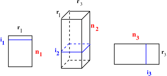
Figure 2.2: A first step in canonical-to-Tucker decomposition.

Here we notice that the core tensor in the RHOSVD decomposition can be represented in the CP data-sparse format.

Proposition 2.2

The core tensor

$${\boldsymbol{\beta}}_{0}=\boldsymbol{\xi}\times_{1}[D_{1,0}{V_{0}^{(1)}}^{T}]\times_{2}\cdots\times_{d}[D_{d,0}{V_{0}^{(d)}}^{T}]\in\mathbb{R}^{r_{1}\times\cdots\times r_{d}},$$

in the orthogonal Tucker representation (2.5), ${\bf A}_{({\bf r})}^{0}={\boldsymbol{\beta}}_{0}\times_{1}Z^{(1)}_{0}\times_{2}\cdots\times_{d}Z^{(d)}_{0}\in\mbox{\boldmath{$\mathcal{T}$}}_{{\bf r},{\bf n}},$ can be recognized as the rank-$R$ canonical tensor of size $r_{1}\times\cdots\times r_{d}$ with the storage request $R(\sum\limits_{\ell=1}^{d}r_{\ell})$, which can be calculated entry-wise in $O(Rr_{1}\cdots r_{d})$ operations.

Indeed, introducing the matrices ${U_{0}^{(\ell)}}^{T}=D_{\ell,0}{V_{0}^{(\ell)}}^{T}\in\mathbb{R}^{r_{\ell}\times R}$, for $\ell=1,\ldots d$, we conclude that the canonical core tensor ${\boldsymbol{\beta}}_{0}$ is determined by the $\ell$-mode side matrices ${U_{0}^{(\ell)}}^{T}$. In the other words, the tensor ${\bf A}_{({\bf r})}^{0}$ is represented in the mixed Tucker-canonical format getting rid of the “curse of dimensionality”, see also §2.2 below.

The accuracy of the RHOSVD approximation can be controlled by the given $\varepsilon$-threshold in truncated SVD of side matrices $U^{(\ell)}$. The following theorem proves the absolute error bound for the RHOSVD approximation.

Theorem 2.3

(RHOSVD error bound, [33]). For given ${\bf A}\in\mbox{\boldmath{$\mathcal{C}$}}_{{R},{\bf n}}$ in (2.1), let $\sigma_{\ell,1}\geq\sigma_{\ell,2}...\geq\sigma_{\ell,\min(n,R)}$ be the singular values of $\ell$-mode side matrices $U^{(\ell)}\in\mathbb{R}^{n\times R}$ ($\ell=1,...,d$) with normalized skeleton vectors. Then the error of RHOSVD approximation, ${\bf A}_{({\bf r})}^{0}$, is bounded by

$$\|{\bf A}-{\bf A}_{({\bf r})}^{0}\|\leq\|\boldsymbol{\xi}\|\sum\limits_{\ell=1}^{d}(\sum\limits_{k=r_{\ell}+1}^{\min(n,R)}\sigma_{\ell,k}^{2})^{1/2},\quad\|\boldsymbol{\xi}\|=\sqrt{\sum\limits_{\nu=1}^{R}\xi_{\nu}^{2}}.$$ (2.7)

Proof. Using the contracted product representations of ${\bf A}\in\mbox{\boldmath{$\mathcal{C}$}}_{{R},{\bf n}}$ and ${\bf A}_{({\bf r})}^{0}\in{\cal T}_{\bf r}$, and introducing the $\ell$-mode residual

$$\Delta^{(\ell)}={U}^{(\ell)}-{Z}_{0}^{(\ell)}D_{\ell,0}{V_{0}^{(\ell)}}^{T},\quad\{\Delta^{(\ell)}\}_{\nu}=\sum\limits_{k=r_{\ell}+1}^{n}\sigma_{\ell,k}{\bf z}^{(\ell)}_{k}v^{\ell}_{k,\nu},\quad\nu=1,...,R,$$

with notations ${V_{0}^{(\ell)}}=[{\bf v}^{(\ell)}_{1},...,{\bf v}^{(\ell)}_{r_{\ell}}]^{T},\quad{\bf v}^{(\ell)}_{k}=\{v^{\ell}_{k,\nu}\}_{\nu=1}^{R}\in\mathbb{R}^{R},$ we arrive at the following expansion for the approximation error in the form

$${\bf A}-{\bf A}_{({\bf r})}^{0}=\boldsymbol{\xi}\times_{1}U^{(1)}\times_{2}\cdots\times_{d}U^{(d)}-\boldsymbol{\xi}\times_{1}W^{(1)}\times_{2}\cdots\times_{d}W^{(d)}:=\sum\limits_{\ell=1}^{d}{\bf B}_{\ell},$$

where

$${\bf B}_{\ell} = \boldsymbol{\xi}\times_{1}{U}^{(1)}\cdots\times_{\ell-1}U^{(\ell-1)}\times_{\ell}\Delta^{(\ell)}\times_{\ell+1}W^{(\ell+1)}\cdots\times_{d}W^{(d)}$$

$$= \sum\limits_{\nu=1}^{R}{\xi}_{\nu}\left[{\bf u}^{(\ell)}_{\nu}\cdots\times_{\ell-1}{\bf u}^{(\ell-1)}_{\nu}\times_{\ell}\{\Delta^{(\ell)}\}_{\nu}\times_{\ell+1}\sum\limits_{k=1}^{r_{\ell+1}}\sigma_{\ell+1,k}{\bf z}^{(\ell+1)}_{k}v^{\ell+1}_{k,\nu}\cdots\times_{d}\sum\limits_{k=1}^{r_{d}}\sigma_{d,k}{\bf z}^{(d)}_{k}v^{d}_{k,\nu}\right].$$

This leads to the error bound (by the triangle inequality)

$$\|{\bf A}-{\bf A}_{({\bf r})}^{0}\|\leq\sum\limits_{\ell=1}^{d}\|{\bf B}_{\ell}\|,$$

providing the estimate (in view of $\|{\bf u}^{(\ell)}_{\nu}\|=1$, $\ell=1,...,d$, $\nu=1,...,R$)

$$\|{\bf B}_{\ell}\|\leq\sum\limits_{\nu=1}^{R}|{\xi}_{\nu}|(\sum\limits_{k=r_{\ell}+1}^{n}\sigma_{\ell,k}^{2}(v^{\ell}_{k,\nu})^{2})^{1/2}\,(\sum\limits_{k=1}^{r_{\ell+1}}\sigma_{\ell+1,k}^{2}(v^{\ell+1}_{k,\nu})^{2})^{1/2}\cdots(\sum\limits_{k=1}^{r_{d}}\sigma_{d,k}^{2}(v^{d}_{k,\nu})^{2})^{1/2}.$$

Furthermore, since $U^{(\ell)}$ has normalized columns, i.e., $\|{\bf u}^{(\ell)}_{\nu}\|=\|\sum\limits_{k=1}^{n}\sigma_{\ell,k}{\bf z}^{(\ell)}_{k}{v^{\ell}_{k,\nu}}\|=1,\quad\ell=1,...,d,$ we obtain $\sum\limits_{k=1}^{n}\sigma_{\ell,k}^{2}(v^{\ell}_{k,\nu})^{2}=1$ for $\ell=1,...,d$ $\nu=1,...,R$. Now the error estimate follows

$$\|{\bf A}-{\bf A}_{({\bf r})}^{0}\| \leq \sum\limits_{\ell=1}^{d}\sum\limits_{\nu=1}^{R}|{\xi}_{\nu}|\left(\sum\limits_{k=r_{\ell}+1}^{n}\sigma_{\ell,k}^{2}(v^{\ell}_{k,\nu})^{2}\right)^{1/2}$$

$$\leq \sum\limits_{\ell=1}^{d}\left(\sum\limits_{\nu=1}^{R}{\xi}_{\nu}^{2}\right)^{1/2}\left(\sum\limits_{\nu=1}^{R}\sum\limits_{k=r_{\ell}+1}^{n}\sigma_{\ell,k}^{2}(v^{\ell}_{k,\nu})^{2}\right)^{1/2}$$

$$= \sum\limits_{\ell=1}^{d}\|\boldsymbol{\xi}\|\left(\sum\limits_{k=r_{\ell}+1}^{n}\sigma_{\ell,k}^{2}\sum\limits_{\nu=1}^{R}(v^{\ell}_{k,\nu})^{2}\right)^{1/2}=\|\boldsymbol{\xi}\|\sum\limits_{\ell=1}^{d}\left(\sum\limits_{k=r_{\ell}+1}^{n}\sigma_{\ell,k}^{2}\right)^{1/2}.$$

The case $R<n$ can be analyzed along the same line.   

The error estimate in Theorem 2.3 differs from the case of complete HOSVD by the extra factor $\|\boldsymbol{\xi}\|$, which is the payoff for the lack of orthogonality in the canonical input tensor. Hence Theorem 2.3 does not provide, in general, the stable control of relative error since for the general canonical tensors there is no uniform upper bound on the constant $C$ in the estimate

$$\|\boldsymbol{\xi}\|\leq C\|{\bf A}\|.$$

The problem is that it applies to the non-orthogonal canonical decomposition. The stable decomposition can be proven in the case of partially orthogonal or monotone decompositions.

Corollary 2.4

(Stability of RHOSVD) Assume the conditions of Theorem 2.3 are satisfied. (A) Suppose that one of the matrices $U^{(\ell)}$, say $U^{(1)}$, is orthogonal. Then the RHOSVD error can be bounded by

$$\|{\bf A}-{\bf A}_{({\bf r})}^{0}\|\leq C\|{\bf A}\|\sum\limits_{\ell=1}^{d}(\sum\limits_{k=r_{\ell}+1}^{\min(n,R)}\sigma_{\ell,k}^{2})^{1/2},$$ (2.8)

with the constant $C=1$.
(B) Let decomposition (2.1) be monotone, i.e. all coefficients and skeleton vectors have non-negative values. Then (2.8) holds with the constant $C$ that does not depend on ${\bf A}$.

Proof. (A) The partial orthogonality assumption combined with normalization constraints for the canonical skeleton vectors imply

$$\sum\limits_{\nu=1}^{R}\xi_{\nu}^{2}=\|\boldsymbol{\xi}\|^{2}=\|{\bf A}\|^{2},$$

then the result follows by (2.7).
(B) In case of monotone decomposition we conclude that the pairwise scalar product of all summands in (2.1) is non-negative, while the norm of each $\nu$-term is equal to $\xi_{\nu}$. Then the result follows by the upper bound

$$(u_{1},u_{1})+\cdots+(u_{R},u_{R})\leq(\sum\limits_{\nu=1}^{R}u_{\nu},\sum u_{\nu}),$$

which holds for vectors with non-negative entries applied in the case of $R$ summands.   

Clearly, the orthogonality assumption may lead to slightly higher separation rank, however, this constructive decomposition stabilizes the RHOSVD approximation method applied to the canonical format tensor (i.e., it allows the stable control of relative error). The case of monotone canonical sums typically arises in the sinc-based canonical approximation to radially symmetric Green’s kernels by a sum of Gaussians. On the other hand, in long term computational practice the numerical instability of RHOSVD approximation was not observed in case of physically relevant data.

2.2 Mixed Tucker tensor format and Tucker-to-CP transform

In the procedure for the canonical tensor rank reduction the goal is to have a result in a canonical tensor format with a smaller rank. By converting the core tensor to CP format, one can use the mixed two-level Tucker data format [32, 26], or canonical CP format. Figure 2.3 illustrates the computational scheme of the two-level Tucker approximation.

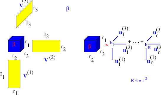
Figure 2.3: Mixed Tucker-to-canonical decomposition.

Next lemma describes the approximation of the Tucker tensor by using canonical representation [32, 26].

Lemma 2.5

(Mixed Tucker-to-canonical approximation, [26]).
(A) Let the target tensor ${\bf A}$ have the form ${\bf A}={\boldsymbol{\beta}}\times_{1}V^{(1)}\times_{2}...\times_{d}V^{(d)}\in\mbox{\boldmath{$\mathcal{T}$}}_{{\bf r},{\bf n}},$ with the orthogonal side-matrices $V^{(\ell)}=[{\bf v}^{(\ell)}_{1}\ldots{\bf v}^{(\ell)}_{r_{\ell}}]\in\mathbb{R}^{n\times r_{\ell}}$ and ${\boldsymbol{\beta}}\in\mathbb{R}^{r_{1}\times...\times r_{d}}$. Then, for a given $R\leq\min\limits_{1\leq\ell\leq d}\overline{r}_{\ell}$,

$$\min\limits_{{\bf Z}\in\mbox{\boldmath{$\mathcal{C}$}}_{R,{\bf n}}}\|{\bf A}-{\bf Z}\|=\min\limits_{{\boldsymbol{\mu}}\in\mbox{\boldmath{$\mathcal{C}$}}_{R,{\bf r}}}\|{\boldsymbol{\beta}}-{\boldsymbol{\mu}}\|,$$ (2.9)

where $\overline{n}_{\ell}$ is the single-hole product of dimension-modes,

$$\overline{n}_{\ell}=n_{1}\cdots n_{\ell-1}n_{\ell+1}\cdots n_{d}$$ (2.10)

. (B) Assume that there exists the best rank-$R$ approximation ${\bf A}_{(R)}\in\mbox{\boldmath{$\mathcal{C}$}}_{R,{\bf n}}$ of ${\bf A}$, then there is the best rank-$R$ approximation ${\boldsymbol{\beta}}_{(R)}\in\mbox{\boldmath{$\mathcal{C}$}}_{R,{\bf r}}$ of ${\boldsymbol{\beta}}$, such that

$${\bf A}_{({R})}={\boldsymbol{\beta}}_{(R)}\times_{1}V^{(1)}\times_{2}...\times_{d}V^{(d)}.$$ (2.11)

Proof. (A) The canonical vectors ${\bf y}_{k}^{(\ell)}$ of any test element on the left-hand side of (2.9),

$${\bf Z}=\sum\limits_{k=1}^{R}\lambda_{k}\;{\bf y}_{k}^{(1)}\otimes...\otimes{\bf y}_{k}^{(d)}\in\mbox{\boldmath{$\mathcal{C}$}}_{R,{\bf n}},$$ (2.12)

can be chosen in $span\{{\bf v}^{(\ell)}_{1},\ldots,{\bf v}^{(\ell)}_{r_{\ell}}\}$, that means

$${\bf y}^{(\ell)}_{k}=\sum\limits_{m=1}^{r_{\ell}}\mu_{k,m}^{(\ell)}{\bf v}^{(\ell)}_{m},\quad k=1,\ldots,R,\;\ell=1,...,d.$$ (2.13)

Indeed, assuming

$${\bf y}^{(\ell)}_{k}=\sum\limits_{m=1}^{r_{\ell}}\mu_{k,m}^{(\ell)}{\bf v}^{(\ell)}_{m}+{\bf e}^{(\ell)}_{k}\quad\mbox{with}\quad{\bf e}^{(\ell)}_{k}\bot span\{{\bf v}^{(\ell)}_{1},\ldots,{\bf v}^{(\ell)}_{r_{\ell}}\},$$

we conclude that ${\bf e}^{(\ell)}_{k}$ does not effect the cost function in (2.9) because of the orthogonality of $V^{(\ell)}$. Hence, setting ${\bf e}^{(\ell)}_{k}=0$, and plugging (2.13) in (2.12), we arrive at the desired Tucker decomposition of ${\bf Z}$, ${\bf Z}=\boldsymbol{\beta}_{z}\times_{1}V^{(1)}\times_{2}\ldots\times_{d}V^{(d)},\quad\boldsymbol{\beta}_{z}\in\mbox{\boldmath{$\mathcal{C}$}}_{R,{\bf r}}.$ This implies

$$\|{\bf A}-{\bf Z}\|^{2}=\|(\boldsymbol{\beta}_{z}-\boldsymbol{\beta})\times_{1}V^{(1)}\times_{2}\ldots\times_{d}V^{(d)}\|^{2}=\|\boldsymbol{\beta}-\boldsymbol{\beta}_{z}\|^{2}\geq\min\limits_{\boldsymbol{\mu}\in\mbox{\boldmath{$\mathcal{C}$}}_{R,{\bf r}}}\|\boldsymbol{\beta}-\boldsymbol{\mu}\|^{2}.$$

On the other hand, we have

$$\min\limits_{{\bf Z}\in\mbox{\boldmath{$\mathcal{C}$}}_{R,{\bf n}}}\|{\bf A}-{\bf Z}\|^{2}\leq\min\limits_{\boldsymbol{\beta}_{z}\in\mbox{\boldmath{$\mathcal{C}$}}_{R,{\bf r}}}\|(\boldsymbol{\beta}-\boldsymbol{\beta}_{z})\times_{1}V^{(1)}\times_{2}\ldots\times_{d}V^{(d)}\|^{2}=\min\limits_{\boldsymbol{\mu}\in\mbox{\boldmath{$\mathcal{C}$}}_{R,{\bf r}}}\|\boldsymbol{\beta}-\boldsymbol{\mu}\|^{2}.$$

This proves (2.9).

(B) Likewise, for any minimizer ${\bf A}_{(R)}\in\mbox{\boldmath{$\mathcal{C}$}}_{R,{\bf n}}$ in the right-hand side in (2.9), one obtains

$${\bf A}_{(R)}=\boldsymbol{\beta}_{(R)}\times_{1}V^{(1)}\times_{2}V^{(2)}...\times_{d}V^{(d)}$$

with the respective rank-$R$ core tensor $\boldsymbol{\beta}_{(R)}=\sum\limits_{k=1}^{R}\lambda_{k}{\bf u}_{k}^{(1)}\otimes...\otimes{\bf u}_{k}^{(d)}\in\mbox{\boldmath{$\mathcal{C}$}}_{R,{\bf r}}.$ Here ${\bf u}_{k}^{(\ell)}=\{\mu_{k,m_{\ell}}^{(\ell)}\}_{m_{\ell}=1}^{r_{\ell}}\in\mathbb{R}^{r_{\ell}}$, are calculated by plugging representation (2.13) in (2.12), and then by changing the order of summation,

$${\bf A}_{(R)} =\sum\limits_{k=1}^{R}\lambda_{k}{\bf y}_{k}^{(1)}\otimes...\otimes{\bf y}_{k}^{(d)}=\sum\limits_{k=1}^{R}\lambda_{k}\left(\sum\limits_{m_{1}=1}^{r_{1}}\mu_{k,m_{1}}^{(1)}{\bf v}^{(1)}_{m_{1}}\right)\otimes...\otimes\left(\sum\limits_{m_{d}=1}^{r_{d}}\mu_{k,m_{d}}^{(d)}{\bf v}^{(d)}_{m_{d}}\right)$$

$$=\sum\limits_{m_{1}=1}^{r_{1}}...\sum\limits_{m_{d}=1}^{r_{d}}\left\{\sum\limits_{k=1}^{R}\lambda_{k}\prod\limits_{\ell=1}^{d}\mu_{k,m_{\ell}}^{(\ell)}\right\}{\bf v}^{(1)}_{m_{1}}\otimes...\otimes{\bf v}^{(d)}_{m_{d}}.$$

Now (2.11) implies that

$$\|{\bf A}-{\bf A}_{R}\|=\|\boldsymbol{\beta}-\boldsymbol{\beta}_{(R)}\|,$$

since the $\ell$-mode multiplication with the orthogonal side matrices $V^{(\ell)}$ does not change the cost functional. Inspection of the left-hand side in (2.9) indicates that the latter equation ensures that $\boldsymbol{\beta}_{(R)}$ is, in fact, the minimizer of the right-hand side in (2.9).   

Combination of Theorem 2.3 and Lemma 2.5 opens the way to the rank optimization of canonical tensors with the large mode-size arising, for example, in the grid-based numerical methods for multidimensional PDEs with non-regular (singular) solutions. In such applications the univariate grid-size (i.e. the mode-size) may be about $n=10^{4}$ and even larger.

Notice that the Tucker (for moderate $d$) and canonical formats allow to perform basic multi-linear algebra using one-dimensional operations, thus reducing the exponential scaling in $d$. Rank-truncated transforms between different formats can be applied in multi-linear algebra on mixed tensor representations as well, see Lemma 2.5. The particular application to tensor convolution in many dimensions was discussed, for example, in [59, 60].

We summarize that the direct methods of tensor approximation can be classified by:

• Analytic Tucker approximation to some classes of function-related $d$th order tensors ($d\geq 2$), say, by multivariate polynomial interpolation [59].

• Sinc quadrature based approximation methods in the canonical format applied to a class of analytic function related tensors [19].

• Truncated HOSVD and RHOSVD, for quasi-optimal Tucker approximation of the full-format, respectively, canonical tensors [33].

Direct analytic approximation methods by sinc quadrature/interpolation are of principal importance. Basic examples are given by the tensor representation of Green’s kernels, the elliptic operator inverse and analytic matrix-valued functions. In all cases the algebraic methods for rank reduction by the ALS-type iterative Tucker/canonical approximation can be applied.

Further improvement and enhancement of algebraic tensor approximation methods can be based on the combination of advanced nonlinear iteration, multigrid tensor methods, greedy algorithms, hybrid tensor representations and the use of new problem adapted tensor formats.

2.3 Tucker-to-canonical transform

In the rank reduction scheme for the canonical rank-$R$ tensors, we use successively the canonical-to-Tucker (C2T) transform and then the Tucker-to-canonical (T2C) tensor approximation.

First, we notice that the canonical rank of a tensor ${\bf A}\in\mathbb{V}_{\bf n}$ has the upper bound, see [26, 33],

$$R\leq\min\limits_{1\leq\ell\leq d}\overline{n}_{\ell},$$ (2.14)

where $\overline{n_{\ell}}$ is given by (2.10). Rank bound (2.14) applied to the Tucker core tensor of the size $r\times r\times r$, indicates that the ultimate canonical rank of a large-size tensor in $\mathbb{V}_{\bf n}$ has the upper bound $r^{2}$.

The following remark shows that the maximal canonical rank of the Tucker core of 3rd order tensor can be easily reduced to the value less than $r^{2}$ by the SVD-based procedure applied to the matrix slices of the Tucker core tensor $\boldsymbol{\beta}$. Though, being not practically attractive for arbitrary high order tensors, the simple algorithm described in Remark 2.6 below is proved to be useful for the treatment of small size 3rd order Tucker core tensors within the rank reduction algorithms described in the previous sections.

Remark 2.6

[26, 33] Let $d=3$ for the sake of clearness. There is a simple procedure based on SVD to reduce the canonical rank of the core tensor $\boldsymbol{\beta}$, within the accuracy $\varepsilon>0$. Denote by $B_{m}\in\mathbb{R}^{r\times r}$, $m=1,\ldots,r$ the two-dimensional slices of $\boldsymbol{\beta}$ in each fixed mode and represent

$$\boldsymbol{\beta}=\sum\limits_{m=1}^{r}B_{m}\otimes{\bf z}_{m},\quad{\bf z}_{m}\in\mathbb{R}^{r},$$ (2.15)

where ${\bf z}_{m}(m)=1$, ${\bf z}_{m}(j)=0$ for $j=1,\ldots,r$, $j\neq m$ (there are exactly $d$ possible decompositions). Let $p_{m}$ be the minimal integer, such that the singular values of $B_{m}$ satisfy $\sigma^{(m)}_{k}\leq\frac{\varepsilon}{r^{3/2}}$ for $k=p_{m}+1,...,r$ (if $\sigma^{(m)}_{r}>\frac{\varepsilon}{r^{3/2}}$, then set $p_{m}=r$). Then, denoting by

$$B_{p_{m}}=\sum\limits_{k_{m}=1}^{p_{m}}\sigma^{(m)}_{k_{m}}{\bf u}_{k_{m}}\otimes{\bf v}_{k_{m}},$$

the corresponding rank-$p_{m}$ approximation to $B_{m}$ (by truncation of $\sigma^{(m)}_{p_{m}+1},\ldots,\sigma^{(m)}_{r}$), we arrive at the rank-$R$ canonical approximation to $\boldsymbol{\beta}$,

$$\boldsymbol{\beta}_{(R)}:=\sum\limits_{m=1}^{r}B_{p_{m}}\otimes{\bf z}_{m},\quad{\bf z}_{m}\in\mathbb{R}^{r},$$ (2.16)

providing the error estimate

$$\|\boldsymbol{\beta}-\boldsymbol{\beta}_{(R)}\|\leq\sum\limits^{r}_{m=1}\|B_{m}-B_{p_{m}}\|=\sum\limits^{r}_{m=1}\sqrt{\sum\limits^{r}_{k_{m}=p_{m}+1}(\sigma^{(m)}_{k_{m}}})^{2}\leq\sum\limits^{r}_{m=1}\sqrt{r\frac{\varepsilon^{2}}{r^{3}}}=\varepsilon$$

Representation (2.16) is a sum of rank-$p_{m}$ terms so that the total rank is bounded by $R\leq p_{1}+...+p_{r}\leq r^{2}$. The approach can be extended to arbitrary $d\geq 3$ with the bound $R\leq r^{d-1}$.

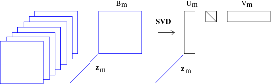
Figure 2.4: Tucker-to-canonical decomposition for a small core tensor, see Remark 2.6.

Figure 2.4 illustrates the canonical decomposition of the core tensor by using the SVD of slices $B_{m}$ of the core tensor $\boldsymbol{\beta}$, yielding matrices $U_{m}=\{{\bf u}_{k_{m}}\}_{k=1}^{p_{m}}$, $V_{m}=\{{\bf v}_{k_{m}}\}_{k=1}^{p_{m}}$ and a diagonal matrix of small size $p_{m}\times p_{m}$ containing the truncated singular values. It also shows the vector ${\bf z}_{m}=[0,\ldots,0,1,0,\ldots,0]$, containing all entries equal to $0$ except $1$ at the m-th position.

3 Calculation of 3D integrals with the Newton kernel

The first application of the RHOSVD was calculation of the 3D grid-based Hartree potential operator in the Hartree-Fock equation,

$${V_{H}({x}):=\int_{\mathbb{R}^{3}}\frac{\rho({y})}{\|{x}-{y}\|}\,d{y}},$$ (3.1)

where the electron density,

$$\rho(x)=2\sum\limits_{a=1}^{N_{orb}}(\varphi_{a})^{2}$$ (3.2)

, is represented in terms of molecular orbitals, presented in the Gaussian-type basis (GTO),

$$\varphi_{a}(x)=\sum\limits_{k=1}^{N_{b}}c_{a,k}g_{k}(x)$$

The Hartree potential describes the repulsion energy of the electrons in a molecule. The intermediate goal here is the calculation of the so-called Coulomb matrix,

$$J_{km}:=\int_{\mathbb{R}^{3}}g_{k}({x})g_{m}({x})V_{H}({x})d{x},\quad k,m=1,\ldots N_{b}\quad x\in\mathbb{R}^{3},$$

which represents the Hartree potential in the given GTO basis.

In fact, calculation of this 3D convolution operator with the Newton kernel, requires high accuracy and it should be repeated multiply in the course of the iterative solution of the Hartree-Fock nonlinear eigenvalue problem. The presence of nuclear cusps in the electron density makes additional challenge to computation of the Hartree potential operator. Traditionally, these calculations are based on involved analytical evaluation of the corresponding integral in a separable Gaussian basis set by using erf function. Tensor-structured calculation of the multidimensional convolution integral operators with the Newton kernel have been introduced in [33, 34, 26].

The molecule is embedded in a computational box $\Omega=[-b,b]^{3}\in\mathbb{R}^{3}$. The equidistant $n\times n\times n$ tensor grid $\omega_{{\bf 3},n}=\{x_{\bf i}\}$, ${\bf i}\in{\cal I}:=\{1,...,n\}^{3}$, with the mesh-size $h=2b/(n+1)$ is used. In calculations of integral terms, the Gaussian basis functions $g_{k}(x),\;x\in\mathbb{R}^{3}$, are approximated by sampling their values at the centers of discretization intervals using one-dimensional piecewise constant basis functions $g_{k}(x)\approx\overline{g}_{k}(x)=\prod^{3}_{\ell=1}\overline{g}_{k}^{(\ell)}(x_{\ell})$, $\ell=1,2,3$, yielding their rank-$1$ tensor representation,

$${\bf G}_{k}={\bf g}_{k}^{(1)}\otimes{\bf g}_{k}^{(2)}\otimes{\bf g}_{k}^{(3)}\in\mathbb{R}^{n\times n\times n},\quad k=1,...,N_{b}.$$ (3.3)

Given the discrete tensor representation of basis functions (3.3), the electron density is approximated using 1D Hadamard products of rank-$1$ tensors as

$$\rho\approx\Theta=2\sum\limits^{N_{orb}}_{a=1}\sum\limits^{N_{b}}_{k=1}\sum\limits^{N_{b}}_{m=1}c_{a,m}c_{a,k}({\bf g}_{k}^{(1)}\odot{\bf g}_{m}^{(1)})\otimes\cdots\otimes({\bf g}_{k}^{(3)}\odot{\bf g}_{m}^{(3)})\in\mathbb{R}^{n\times n\times n}.$$ (3.4)

For convolution operator, the representation of the Newton kernel $\frac{1}{\|{x}-{y}\|}$ by a canonical rank-$R_{N}$ tensor [59] is used (see section 4.1 for details),

$${\bf P}_{R}=\sum\limits_{q=1}^{R_{N}}{\bf p}^{(1)}_{q}\otimes{\bf p}^{(2)}_{q}\otimes{\bf p}^{(3)}_{q}\in\mathbb{R}^{n\times n\times n}.$$ (3.5)

The initial rank of the electron density in the canonical tensor format $\Theta$ in (3.2) is large even for small molecules. Rank reduction by using RHOSVD C2T plus T2C reduces the rank $\Theta\mapsto\Theta^{\prime}$ by several orders of magnitude, from $N_{b}^{2}/2$ to $R_{\rho}\ll N_{b}^{2}/2$, from $\sim 10^{4}$ to $\sim 10^{2}$ . Then the 3D tensor representation of the Hartree potential is calculated by using the 3D tensor product convolution, which is a sum of tensor products of 1D convolutions,

$$V_{H}\approx{\bf V}_{H}=\Theta^{\prime}\ast{\bf P}_{R}=\sum\limits_{m=1}^{R_{\rho}}\sum\limits_{q=1}^{R_{N}}c_{m}\left({\bf u}^{(1)}_{m}\ast{\bf p}^{(1)}_{q}\right)\otimes\left({\bf u}^{(2)}_{m}\ast{\bf p}^{(2)}_{q}\right)\otimes\left({\bf u}^{(3)}_{m}\ast{\bf p}^{(3)}_{q}\right).$$

The Coulomb matrix entries $J_{km}$ are obtained by 1D scalar products of ${\bf V}_{H}$ with the Galerkin basis consisting of rank-$1$ tensors,

$$J_{km}\approx\langle{\bf G}_{k}\odot{\bf G}_{m},{\bf V}_{H}\rangle,\quad k,m=1,\ldots N_{b}.$$

The cost of 3D tensor product convolution is $O(n\log n)$ instead of $O(n^{3}\log n)$ for the standard benchmark 3D convolution using the 3D FFT. Table 3.1 shows CPU times (sec) for the Matlab computation of $V_{H}$ for H₂O molecule [33] on a SUN station using 8 Opteron Dual-Core/2600 processors (times for 3D FFT for $n\geq 1024$ are obtained by extrapolation). C2T shows the time for the canonical-to-Tucker rank reduction.

The grid-based tensor calculation of the multidimensional integrals in quantum chemistry provides the required high accuracy by using large grids and the ranks are controlled by the required $\varepsilon$ in the rank truncation algorithms. The results of the tensor-based calculations have been compared with the results of the benchmark standard computations by the MOLPRO package. It was shown that the accuracy is of the order of $10^{-7}$ hartree in the resulting ground state energy, see [26, 60].

$n^{3}$	$1024^{3}$	$2048^{3}$	$4096^{3}$	$8192^{3}$	$16384^{3}$
FFT3	$\sim 6000$	–	–	–	$\sim 2$ years
$C\ast C$	$8.8$	$20.0$	$61.0$	$157.5$	$299.2$
C2T	$6.9$	$10.9$	$20.0$	$37.9$	$86.0$

Table 3.1: Times (sec) for the C2T transform and the 3D tensor product convolution vs. 3D FFT convolution.

4 RHOSVD in the range-separated tensor formats

The range-separated (RS) tensor formats have been introduced in [3] as the constructive tool for low-rank tensor representation (approximation) of function related data discretized on Cartesian grids in $\mathbb{R}^{d}$, which may have multiple singularities or cusps. Such highly non-regular data typically arise in computational quantum chemistry, in many-particle dynamics simulations and many-particle electrostatics calculations, in protein modeling and in data science. The key idea of the RS representation is the splitting of the short- and long-range parts in the functional data and further low-rank approximation of the rather regular long-range part in the classical tensor formats.

In this concern RHOSVD method becomes an essential ingredient of the rank reduction algorithms for the “long-range” input tensor, which usually inherits the large initial rank.

4.1 Low-rank approximation of radial functions

First, we recall the grid-based method for the low-rank canonical representation of a spherically symmetric kernel functions $p(\|x\|)$, $x\in\mathbb{R}^{d}$ for $d=2,3,\ldots$, by its projection onto the finite set of basis functions defined on tensor grid. The approximation theory by a sum of Gaussians for the class of analytic potentials $p(\|x\|)$ was presented in [55, 19, 29, 59]. The particular numerical schemes for rank-structured representation of the Newton and Slater kernels

$$p(\|x\|)=\frac{1}{4\pi\|x\|},\quad\mbox{ and }\quad p(\|x\|)=e^{-\lambda\|x\|},\quad x\in\mathbb{R}^{3},$$ (4.1)

discretized on a fine 3D Cartesian grid in the form of low-rank canonical tensor was described in [19, 29].

In what follows, for the ease of exposition, we confine ourselves to the case $d=3$. In the computational domain $\Omega=[-b,b]^{3}$, let us introduce the uniform $n\times n\times n$ rectangular Cartesian grid $\Omega_{n}$ with mesh size $h=2b/n$ ($n$ even). Let $\{\psi_{\textbf{i}}=\prod_{\ell=1}^{3}\psi_{i_{\ell}}^{(\ell)}(x_{\ell})\}$ be a set of tensor-product piecewise constant basis functions, labeled by the $3$-tuple index ${\bf i}=(i_{1},i_{2},i_{3})$, $i_{\ell}\in I_{\ell}=\{1,...,n\}$, $\ell=1,\,2,\,3$. The generating kernel $p(\|x\|)$ is discretized by its projection onto the basis set $\{\psi_{\textbf{i}}\}$ in the form of a third order tensor of size $n\times n\times n$, defined entry-wise as

$$\mathbf{P}:=[p_{\bf i}]\in\mathbb{R}^{n\times n\times n},\quad p_{\bf i}=\int_{\mathbb{R}^{3}}\psi_{\bf i}({x})p(\|{x}\|)\,\,\mathrm{d}{x}.$$ (4.2)

The low-rank canonical decomposition of the $3$rd order tensor $\mathbf{P}$ is based on using exponentially fast convergent $\operatorname*{sinc}$-quadratures for approximating the Laplace-Gauss transform to the analytic function $p(z)$, $z\in\mathbb{C}$, specified by a certain weight $\widehat{p}(t)>0$,

$$p(z)=\int_{\mathbb{R}_{+}}\widehat{p}(t)e^{-t^{2}z^{2}}\,\mathrm{d}t\approx\sum_{k=-M}^{M}p_{k}e^{-t_{k}^{2}z^{2}}\quad\mbox{for}\quad|z|>0,\quad z\in\mathbb{R},$$ (4.3)

with the proper choice of the quadrature points $t_{k}$ and weights $p_{k}$. The $sinc$-quadrature based approximation to generating function by using the short-term Gaussian sums in (4.3) are applicable to the class of analytic functions in certain strip $|z|\leq D$ in the complex plane, such that on the real axis these functions decay polynomially or exponentially. We refer to basic results in [55, 6, 19], where the exponential convergence of the $sinc$-approximation in the number of terms (i.e., the canonical rank) was analyzed for certain classes of analytic integrands.

Now, for any fixed $x=(x_{1},x_{2},x_{3})\in\mathbb{R}^{3}$, such that $\|{x}\|>a>0$, we apply the $\operatorname*{sinc}$-quadrature approximation (4.3) to obtain the separable expansion

$$p({\|{x}\|})=\int_{\mathbb{R}_{+}}\widehat{p}(t)e^{-t^{2}\|{x}\|^{2}}\,\mathrm{d}t\approx\sum_{k=-M}^{M}p_{k}e^{-t_{k}^{2}\|{x}\|^{2}}=\sum_{k=-M}^{M}p_{k}\prod_{\ell=1}^{3}e^{-t_{k}^{2}x_{\ell}^{2}},$$ (4.4)

providing an exponential convergence rate in $M$,

$$\left|p({\|{x}\|})-\sum_{k=-M}^{M}p_{k}e^{-t_{k}^{2}\|{x}\|^{2}}\right|\leq\frac{C}{a}\,\displaystyle{e}^{-\beta\sqrt{M}},\quad\text{with some}\ C,\beta>0.$$ (4.5)

In the case of Newton kernel, we have $p(z)=1/z$, $\widehat{p}(t)=\frac{2}{\sqrt{\pi}}$, so that the Laplace-Gauss transform representation reads

$$\frac{1}{z}=\frac{2}{\sqrt{\pi}}\int_{\mathbb{R}_{+}}e^{-z^{2}t^{2}}dt,\quad\mbox{where}\quad z=\|x\|,\quad x\in\mathbb{R}^{3},$$ (4.6)

which can be approximated by the sinc quadrature (4.4) with the particular choice of quadrature points $t_{k}$, providing the exponential convergence rate as in (4.5), [19, 29].

In the case of Yukawa potential the Laplace Gauss transform reads

$$\frac{e^{-\kappa z}}{z}=\frac{2}{\sqrt{\pi}}\int_{\mathbb{R}_{+}}e^{-\kappa^{2}/t^{2}}e^{-z^{2}t^{2}}dt,\quad\mbox{where}\quad z=\|x\|,\quad x\in\mathbb{R}^{3}.$$ (4.7)

The analysis of the sinc quadrature approximation error for this case can be found, in particular, in [29, 59], §2.4.7.

Combining (4.2) and (4.4), and taking into account the separability of the Gaussian basis functions, we arrive at the low-rank approximation to each entry of the tensor $\mathbf{P}=[p_{\bf i}]$,

$$p_{\bf i}\approx\sum_{k=-M}^{M}p_{k}\int_{\mathbb{R}^{3}}\psi_{\bf i}({x})e^{-t_{k}^{2}\|{x}\|^{2}}\mathrm{d}{x}=\sum_{k=-M}^{M}p_{k}\prod_{\ell=1}^{3}\int_{\mathbb{R}}\psi^{(\ell)}_{i_{\ell}}(x_{\ell})e^{-t_{k}^{2}x^{2}_{\ell}}\mathrm{d}x_{\ell}.$$

Define the vector (recall that $p_{k}>0$)

$$\textbf{p}^{(\ell)}_{k}=p_{k}^{1/3}\left[b^{(\ell)}_{i_{\ell}}(t_{k})\right]_{i_{\ell}=1}^{n_{\ell}}\in\mathbb{R}^{n_{\ell}}\quad\text{with }\quad b^{(\ell)}_{i_{\ell}}(t_{k})=\int_{\mathbb{R}}\psi^{(\ell)}_{i_{\ell}}(x_{\ell})e^{-t_{k}^{2}x^{2}_{\ell}}\mathrm{d}x_{\ell},$$ (4.8)

then the $3$rd order tensor $\mathbf{P}$ can be approximated by the $R$-term ($R=2M+1$) canonical representation

$$\mathbf{P}\approx\mathbf{P}_{R}=\sum_{k=-M}^{M}p_{k}\bigotimes_{\ell=1}^{3}{\bf b}^{(\ell)}(t_{k})=\sum\limits_{k=-M}^{M}{\bf p}^{(1)}_{k}\otimes{\bf p}^{(2)}_{k}\otimes{\bf p}^{(3)}_{k}\in\mathbb{R}^{n\times n\times n},\quad{\bf p}^{(\ell)}_{k}\in\mathbb{R}^{n}.$$ (4.9)

Given a threshold $\varepsilon>0$, in view of (4.5), we can chose $M=O(\log^{2}\varepsilon)$ such that in the max-norm

$$\|\mathbf{P}-\mathbf{P}_{R}\|\leq\varepsilon\|\mathbf{P}\|.$$

In the case of continuous radial function $p({\|{x}\|})$, say the Slater potential, we use the collocation type discretization at the grid points including the origin, $x=0$, so that the univariate mode size becomes $n\to n_{1}=n+1$. In what follows, we use the same notation $\mathbf{P}_{R}$ in the case of collocation type tensors (for example, the Slater potential) so that the particular meaning becomes clear from the context.

4.2 The RS tensor format revisited

The range separated (RS) tensor format was introduced in [3] for efficient representation of the collective free-space electrostatic potential of large biomolecules. This rank-structured tensor representation of the collective electrostatic potential of many-particle systems of general type allows to reduce essentially computation of their interaction energy, and it provides convenient form for performing other algebraic transforms. The RS format proved to be useful for range-separated tensor representation of the Dirac delta [31] in $\mathbb{R}^{d}$ and based on that, for regularization of the Poisson-Boltzmann equation (PBE) by decomposition of the solution into short- and long-range parts, where the short-range part of the solution is evaluated by simple tensor operations without solving the PDE. The smooth long-range part is calculated by solving the PBE with the modified right-hand side by using the RS decomposition of the Dirac delta, so that now it does not contain singularities. We refer to papers [4, 38] describing the approach in details.

First, we recall the definition of the range separated (RS) tensor format, see [3], for representation of $d$-tensors ${\bf A}\in\mathbb{R}^{n_{1}\times\cdots\times n_{d}}$. The RS format is served for the hybrid tensor approximation of discretized functions with multiple cusps or singularities. This allows the splitting of the target tensor onto the highly localized components approximating the singularity and the component with global support that allows the low-rank tensor approximation. Such functions typically arise in computational quantum chemistry, in many-particle modeling and in the interpolation of multidimensional data measured at certain set of spacial points in $\mathbb{R}^{n\times n\times n}$.

Definition 4.1

(RS-canonical tensors, [3]). The RS-canonical tensor format defines the class of $d$-tensors ${\bf A}\in\mathbb{R}^{n_{1}\times\cdots\times n_{d}}$, represented as a sum of a rank-${R_{l}}$ CP tensor ${\bf U}_{long}={\sum}_{k=1}^{R_{l}}\xi_{k}{\bf u}_{k}^{(1)}\otimes\cdots\otimes{\bf u}_{k}^{(d)},$ and a cumulated CP tensor ${\bf U}_{short}={\sum}_{\nu=1}^{N_{0}}c_{\nu}{\bf U}_{\nu}$, such that

$${\bf A}={\bf U}_{long}+{\bf U}_{short}={\sum}_{k=1}^{R_{l}}\xi_{k}{\bf u}_{k}^{(1)}\otimes\cdots\otimes{\bf u}_{k}^{(d)}+{\sum}_{\nu=1}^{N_{0}}c_{\nu}{\bf U}_{\nu},$$ (4.10)

where ${\bf U}_{short}$ is generated by the localized reference CP tensor ${\bf U}_{0}$, i.e., ${\bf U}_{\nu}=\mbox{Replica}({\bf U}_{0})$, with $\mbox{rank}({\bf U}_{\nu})=\mbox{rank}({\bf U}_{0})\leq R_{s}$, where, given the threshold $\delta>0$, the effective support of ${\bf U}_{\nu}$ is bounded by $\mbox{diam}(\mbox{supp}{\bf U}_{\nu})\leq 2n_{\delta}$ in the index size, where $n_{\delta}=O(1)$ is a small integer.

Each RS-canonical tensor is, therefore, uniquely defined by the following parametrization: rank-$R_{l}$ canonical tensor ${\bf U}_{long}$, the rank-$R_{s}$ reference canonical tensor ${\bf U}_{0}$ with the small mode size bounded by $2n_{\delta}$, list ${\cal J}$ of the coordinates and weights of $N_{0}$ particles in $\mathbb{R}^{d}$. The storage size is linear in both the dimension and the univariate grid size,

$$\mbox{stor}({\bf A})\leq dR_{l}n+(d+1)N_{0}+dR_{s}n_{\delta}.$$

The main benefit of the RS-canonical tensor decomposition is the almost uniform bound on the CP/Tucker rank of the long-range part ${\bf U}_{long}={\sum}_{k=1}^{R_{l}}\xi_{k}{\bf u}_{k}^{(1)}\otimes\cdots\otimes{\bf u}_{k}^{(d)}$, in the multi-particle potential discretized on fine $n\times n\times n$ spatial grid. It was proven in [3] that the canonical rank $R$ scales logarithmically in both the number of particles $N_{0}$ and the approximation precision, see also Lemma 4.5.

Given the rank-$R$ CP decomposition (4.9) based on the sinc-quadrature approximation (4.4) of the discretized radial function $p(\|{x}\|)$, we define the two subsets of indices, ${\cal K}_{l}:=\{k:t_{k}\leq 1\}$ and ${\cal K}_{s}:=\{k:t_{k}>1\}$, and then introduce the RS-representation of this tensor as follows,

$${\bf P}_{R}={\bf P}_{R_{l}}+{\bf P}_{R_{s}},\quad R=R_{l}+R_{s},\quad R_{l}=\#{\cal K}_{l},\quad R_{s}=\#{\cal K}_{s},$$ (4.11)

where

$${\bf P}_{R_{l}}:=\sum\limits_{k\in{\cal K}_{l}}{\bf p}^{(1)}_{k}\otimes{\bf p}^{(2)}_{k}\otimes{\bf p}^{(3)}_{k},\quad{\bf P}_{R_{s}}:=\sum\limits_{k\in{\cal K}_{s}}{\bf p}^{(1)}_{k}\otimes{\bf p}^{(2)}_{k}\otimes{\bf p}^{(3)}_{k}.$$

This representation allows to reduce the calculation of the multiparticle interaction energy of the many-particle system. Recall that the electrostatic interaction energy of $N$ charged particles is represented in the form

$$E_{N}=E_{N}(x_{1},\dots,x_{N})=\sum^{N}_{i=1}\sum^{N}_{j<i}\frac{z_{i}z_{j}}{\|x_{i}-x_{j}\|},$$ (4.12)

and it can be computed by direct summation in $O(N^{2})$ operations. The following statement is the modification of Lemma 4.2 in [3], see [28] for more details.

Lemma 4.2

[28] Let the effective support of the short-range components in the reference potential ${\bf P}_{R}$ for the Newton kernel does not exceed the minimal distance between particles, $\sigma>0$. Then the interaction energy $E_{N}$ of the $N$-particle system can be calculated by using only the long range part in the tensor ${\bf P}$ representing on the grid the total potential sum,

$$E_{N}=\frac{1}{2}\sum\limits_{{j}=1}^{N}z_{j}({\bf P}_{l}({x}_{j})-z_{j}{\bf P}_{R_{l}}(0))=\frac{1}{2}\langle{\bf z},{\bf p}_{l}\rangle-\frac{{\bf P}_{R_{l}}(0)}{2}\sum\limits_{{j}=1}^{N}z_{j}^{2},$$ (4.13)

in $O(R_{l}N)$ operations, where $R_{l}$ is the canonical rank of the long-range component in ${\bf P}$, ${\bf P}_{l}$.

Here ${\bf z}\in\mathbb{R}^{N}$ is a vector composed of all charges of the multi-particle systems, and ${\bf p}_{l}\in\mathbb{R}^{N}$ is the vector of samples of the collective electrostatic long-range potential ${\bf P}_{l}$ in the nodes corresponding to particle locations. Thus, the term $\frac{1}{2}\langle{\bf z},{\bf p}_{l}\rangle$ denotes the ”non-calibrated” interaction energy associated with the long-range tensor component ${\bf P}_{l}$, while ${\bf P}_{R_{l}}$ denotes the long-range part in the tensor representing the single reference Newton kernel, and ${\bf P}_{R_{l}}(0)$ is its value at the origin.

Lemma 4.2 indicates that the interaction energy does not depend on the short-range part in the collective potential, and this is the key point for the construction of energy preserving regularized numerical schemes for solving the basic equations in bio-molecular modeling by using low-rank tensor decompositions.

4.3 Multilinear operations in RS tensor formats

In what follows, we address the important question on how the basic multilinear operations can be implemented in the RS tensor format by using the RHOSVD rank compression. The point is that various tensor operations arise in the course of commonly used numerical schemes and iterative algorithms which usually include many sums and products of functions as well as the actions of differential/integral operators, always making the tensor structure of input data much more complicated requiring the robust rank reduction schemes.

The other important aspect is related to the use of large (fine resolution) discretization grids which is limited by the restriction on the size of the full input tensors, $O(n^{d})$ (curse of dimensionality), representing the discrete functions and operators to be approximated in low rank tensor format. Remarkably, that tensor decomposition for special class of functions, which allow the sinc-quadrature approximation, can be performed on practically indefinitely large grids because the storage and numerical costs of such numerical schemes scale linearly in the univariate grid size, $O(dn)$. Hence, having constructed such low rank approximations for certain set of “reproducing” radial functions, makes it possible to construct the low rank RS representation at linear complexity, $O(dn)$, for the wide class of functions and operators by using the rank truncated multilinear operations. The examples of such “reproducing” radial functions are commonly used in our computational practice.

First, consider the Hadamard product of two tensors ${\bf P}_{R}$ and ${\bf Q}_{R_{1}}$ corresponding to the pointwise product of two generating multivariate functions centered at the same point. The RS representation of the product tensor is based on the observation that the long-range part of the Hadamard product of two tensors in RS-format is basically determined by the product of their long-range parts.

Lemma 4.3

Suppose that the RS representation (4.11) of tensors ${\bf P}_{R}$ and ${\bf Q}_{R_{1}}$ is constructed based on the sinc-quadrature CP approximation (4.9). Then the long-range part of the Hadamard product of these RS-tensors,

$${\bf Z}=({\bf P}_{s}+{\bf P}_{l})\odot({\bf Q}_{s}+{\bf Q}_{l}),$$

can be represented by the product of their long-range parts, ${\bf Z}_{l}={\bf P}_{l}\odot{\bf Q}_{l}$, with the subsequent rank reduction. Moreover, we have $rank({\bf Z}_{l})\leq R_{l}Q_{l}$.

Proof. We consider the case of collocation tensors and suppose that each skeleton vector in CP tensors ${\bf P}_{R}$ and ${\bf Q}_{R_{1}}$ is given by the restriction of certain Gaussians to the set of grid points. Chose the arbitrary short-range components in ${\bf P}_{R}$ and some component in ${\bf Q}_{R_{1}}$, generated by Gaussians $e^{-t_{k}x_{\ell}^{2}}$ and $e^{-t_{m}x_{\ell}^{2}}$, respectively. Then the effective support of the product of these two terms becomes smaller than that for each of the factors in view of the identity $e^{-t_{k}x_{\ell}^{2}}e^{-t_{m}x_{\ell}^{2}}=e^{-(t_{k}+t_{m})x_{\ell}^{2}}$ considered for arbitrary $t_{k},t_{m}>0$. This means that each term that includes the short-range multiple remains to be in the short range. Then the long range part in ${\bf Z}$ takes a form ${\bf Z}_{l}={\bf P}_{l}\odot{\bf Q}_{l}$ with the subsequent rank reduction.   

The sums of several tensors in RS format can be easily split into short- and long-range parts by grouping the respective components in the summands. The other important operation is the operator-function product in RS tensor format (see the example in [31] related to the action of Laplacian with the singular Newton kernel resulting in the RS decomposition of the Dirac delta). This topic will be considered in detail elsewhere.

4.4 Representing the Slater potential in RS tensor format

In what follows, we consider the RS-canonical tensor format for the rank-structured representation of the Slater function

$$G(x)=e^{-\lambda\|x\|},\quad\lambda\in\mathbb{R}_{+},$$

which has the principal significance in electronic structure calculations (say, based on the Hartree-Fock equation) since it represents the cusp behavior of electron density in the local vicinity of nuclei. This function (or its approximation) is considered as the best candidate to be used as the localized basis function for atomic orbitals basis sets. Another direction is related to the construction of the accurate low-rank global interpolant for big scattered data to be considered in the next section. In this way, we calculate the data adaptive basis set living on the fine Cartesian grid in the region of target data. The main challenge, however, is due to the presence of point singularities which are hard to approximate in the problem independent polynomial or trigonometric basis sets.

The construction of low-rank RS approximation to the Slater function is based on the generalized Laplace transform representation for the Slater function written in the form $G(\rho)={e^{-2\sqrt{\alpha\rho}}}$, $\rho(x)=x_{1}^{2}+...+x_{d}^{2}$, reads

$$G(\rho)={e^{-2\sqrt{\alpha\rho}}}=\frac{\sqrt{\alpha}}{\sqrt{\pi}}\int_{\mathbb{R}_{+}}\tau^{-3/2}\exp(-\alpha/\tau-\rho\tau)d\tau,$$

which corresponds to the choice $\widehat{G}(\tau)=\frac{\sqrt{\alpha}}{\sqrt{\pi}}\tau^{-3/2}e^{-\alpha/\tau}$ in the canonical form of the Laplace transform representation for $G(\rho)$,

$$G(\rho)=\int_{\mathbb{R}_{+}}\widehat{G}(\tau)e^{-\rho\tau}d\tau.$$ (4.14)

Denote by ${\bf G}_{R}$ the rank-$R$ canonical approximation to the function $G(\rho)$ discretized on the $n\times n\times n$ Cartesian grid.

Lemma 4.4

([29]) For given threshold $\varepsilon>0$ let $\rho\in[1,A]$. Then the $(2M+1)$-term sinc-quadrature approximation of the integral in (4.14) with

$$M=O(|\log\varepsilon|(|\log\varepsilon|+\log A)),$$

ensures the max-error of the order of $O(\varepsilon)$ for the corresponding rank-$(2M+1)$ CP approximation ${\bf G}_{R}$ to the tensor ${\bf G}$.

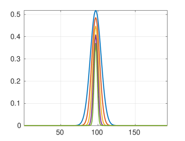
Figure 4.1: Long-range (left) and short-range (right, logarithmic scale) canonical vectors for the Slater function with the grid size $n=1024$, $R=24,R_{l}=6$, $\lambda=1$.

Figure 4.1 illustrates the RS splitting for the tensor ${\bf G}_{R}={\bf G}_{R_{l}}+{\bf G}_{R_{s}}$ representing the Slater potential $G(x)=e^{-\lambda\|x\|}$, $\lambda=1$, discretized on the $n\times n\times n$ grid with $n=1024$. The rank parameters are chosen by $R=24,R_{l}=6$ and $R_{s}=18$. Notice that for this radial function the long-range part (Figure 4.1, left) includes much less canonical vectors comparing with the case of Newton kernel. This anticipates the smaller total canonical rank for the long-range part in the large sum of Slater-like potentials arising, for example, in the representation of molecular orbitals and the electron density in electronic structure calculations. For instance, the wave function for the Hydrogen atom is given by the Slater function $e^{-\mu\|x\|}$. In the following section, we consider the application of RS tensor format to interpolation of scattered data in $\mathbb{R}^{d}$.

4.5 Application of RHOSVD to scattered data modeling

In scattered data modeling the problem is in a low parametric approximation of multi-variate functions $f:\mathbb{R}^{d}\to\mathbb{R}$ by sampling at a finite set ${\cal X}=\{x_{1},\ldots,x_{N}\}\subset\mathbb{R}^{d}$ of piecewise distinct points. Here the function $f$ might be the surface of a solid body, the solution of a PDE, many-body potential field, multi-parametric characteristics of physical systems, or some other multi-dimensional data, etc.

Traditional ways of recovering $f$ from a sampling vector $f_{|{\cal X}}=(f(x_{1}),\ldots,f(x_{N}))$ is the constructing a functional interpolant $P_{N}:\mathbb{R}^{d}\to\mathbb{R}$ such that $P_{N|{\cal X}}=f_{|{\cal X}}=:{\bf f}\in\mathbb{R}^{N}$, i.e.,

$$P_{N}(x_{j})=f(x_{j}),\quad\forall\;1\leq j\leq N.$$ (4.15)

Using radial basis (RB) functions one can find interpolants $P_{N}$ in the form

$$P_{N}(x)=\sum_{j=1}^{N}c_{j}p(\|x-x_{j}\|)+Q(x),\quad Q\;\mbox{is some smooth function, say, polynomial},$$ (4.16)

where $p=p(r):[0,\infty)\to\mathbb{R}$ is a fixed RB function, and $r=\|\cdot\|$ is the Euclidean norm on $\mathbb{R}^{d}$. In further discussion we set $Q(x)=0$. For example, the following RB functions are commonly used

$$p=r^{\nu},\quad(1+r^{2})^{\nu},\;(\nu\in\mathbb{R}),\quad\exp(-r^{2}),\quad\exp(-\lambda r),\quad r^{2}\log(r).$$

The other examples of RB functions are defined by Green’s kernels or by the class of Matérn functions [40].

We discuss the following computational tasks (A) and (B).

• Fixed coefficient vector ${\bf c}=(c_{1},\ldots,c_{N})^{T}\in\mathbb{R}^{N}$, efficiently representing the interpolant $P_{N}(x)$ on the fine tensor grid in $\mathbb{R}^{d}$ providing
  (a) $O(1)$-fast point evaluation of $P_{N}$ in the computational volume $\Omega$,
  (b) computation of various integral-differential operations on that interpolant (say, gradients, scalar products, convolution integrals, etc.).

• Finding the coefficient vector ${\bf c}$ that solves the interpolation problem (4.15) in the case of large number $N$.

Problem (A) exactly fits the RS tensor framework so that the RS tensor approximation solves the problem with low computational costs provided that the sum of long-range parts of the interpolating functions can be easily approximated in the low rank CP tensor format. We consider the case of interpolation by Slater functions $\exp(-\lambda r)$ in the more detail.

Problem (B): Suppose that we use some favorable preconditioned iteration for solving coefficient vector ${\bf c}=(c_{1},\ldots,c_{N})^{T}$,

$$A_{p,{\cal X}}{\bf c}={\bf f},\quad\mbox{with}\quad A_{p,{\cal X}}=A_{p,{\cal X}}^{T}=[p(\|x_{i}-x_{j}\|)]_{1\leq i,j\leq N}\in\mathbb{R}^{N\times N},$$ (4.17)

with the distance dependent symmetric system matrix $A_{p,{\cal X}}$. We assume ${\cal X}=\Omega_{h}$ be the $n^{\otimes d}$-set of grid-points located on tensor grid, i.e., $N=n^{d}$. Introduce the $d$-tuple multi-index $i\mapsto{\bf i}=(i_{1},\ldots,i_{d})$, and $j\mapsto{\bf j}=(j_{1},\ldots,j_{d})$ and reshape $A_{p,{\cal X}}$ into the tensor form

$$A_{p,{\cal X}}\mapsto{\bf A}=[a(i_{1},j_{1},\ldots,i_{d},j_{d})]\in{\bigotimes}_{\ell=1}^{d}\mathbb{R}^{n\times n},$$

which can be decomposed by using the RS based splitting

$${\bf A}={\bf A}_{R_{s}}+{\bf A}_{R_{l}},$$

generated by the RS representation of the weighted potential sum in (4.16). Here ${\bf A}_{R_{s}}$ is (almost) diagonal matrix, while ${\bf A}_{R_{l}}={\sum}_{k=1}^{R_{l}}A^{(1)}_{k}\otimes\cdots\otimes A^{(d)}_{k}$ is the low Kronecker rank matrix. This implies a bound on the storage, $O(N+dR_{l}n)$, and ensures a fast matrix-vector multiplication. Introducing the additional rank-structured representation in ${\bf c}$, the solution of (4.17) can be further simplified.

The above approach can be applied to the data sparse representation for the class of large covariance matrices in the spacial statistics, see for example [43, 40].

In application of tensor methods to data modeling (see §4.5) we consider the interpolation of 3D scattered data by a large sum of Slater functions

$$G_{N}(x)=\sum_{j=1}^{N}c_{j}e^{-\lambda\|x-x_{j}\|},\quad\lambda>0.$$ (4.18)

Given the coefficients $c_{j}$, we address the question how to efficiently represent the interpolant $G_{N}(x)$ on fine Cartesian grid in $\mathbb{R}^{3}$ by using the low-rank (i.e., low-parametric) CP tensor format, such that each value on the grid can be calculated in $O(1)$ operations. The main problem is that the generating Slater function $e^{-\lambda\|x\|}$ has the cusp at the origin so that the considered interpolant has very low regularity. As result, the tensor rank of the function $G_{N}(x)$ in (4.18) discretized on a large $n\times n\times n$ grid increases proportionally to the number $N$ of sampling points $x_{j}$, which in general may be very large. Hence the straightforward tensor approximation of $G_{N}(x)$ does not work in this case.

The generating Slater radial function can be proven to have the low-rank RS canonical tensor decomposition by using the sinc-approximation method, see §4.1.

To complete this section, we present the numerical example demonstrating the application of RS tensor representation to scattered data modeling in $\mathbb{R}^{3}$. We denote by ${\bf G}_{R}\in\mathbb{R}^{n\otimes 3}$ the rank-$R$ CP tensor approximation of the reference Slater potential $e^{-\lambda\|x\|}$ discretized on $n\times n\times n$ grid $\Omega_{n}$, and introduce its RS splitting ${\bf G}_{R}={\bf G}_{R_{l}}+{\bf G}_{R_{s}}$, with $R_{l}+R_{s}=R$. Here $R_{l}\approx R/2$ is the rank parameter of the long-range part in ${\bf G}_{R}$. Assume that all measurement points $x_{j}$ in (4.18) are located on the discretization grid $\Omega_{n}$, then the tensor representation of the long-range part of the total interpolant $P_{N}$ can be obtained as the sum of the properly replicated reference potential ${\bf G}_{l}$, via the shift-and-windowing transform ${\cal W}_{j}$, $j=1,\ldots,N$,

$${\bf G}_{N,l}=\sum_{j=1}^{N}c_{j}{\bf G}_{l,j},\quad{\bf G}_{l,j}={\cal W}_{j}{\bf G}_{l},$$ (4.19)

that includes about $N\,R_{l}$ terms. For large number of measurement points, $N$, the rank reduction is ubiquitous.

It can be proven (by slight modification of arguments in [3]) that both the CP and Tucker ranks of the $N$-term sum in (4.19) depend only logarithmically (but not linearly) on $N$.

Proposition 4.5

(Uniform rank bounds for the long-range part in the Slater interpolant). Let the long-range part ${\bf G}_{N,l}$ in the total Slater interpolant in (4.19) be composed of those terms in (4.4) which satisfy the relation $t_{k}\leq 1$, where $M=O(\log^{2}\varepsilon)$. Then the total $\varepsilon$-rank ${\bf r}_{0}$ of the Tucker approximation to the canonical tensor sum ${\bf G}_{N,l}$ is bounded by

$$|{\bf r}_{0}|:=rank_{Tuck}({\bf G}_{N,l})=C\,b\,\log^{3/2}(\log(N/\varepsilon)),$$ (4.20)

where the constant $C$ does not depend on the number of particles $N$, as well as on the size of the computational box, $[-b,b]^{3}$.

Proof. (Sketch) The main argument of the proof is based on the fact that the grid function ${\bf G}_{N,l}$ has the band-limited Fourier image, such that the frequency interval depends weakly (logarithmically) on $N$. Then we represent all Gaussians in the truncated Fourier basis and make the summation in the fixed set of orthogonal trigonometric basis functions, which defines the orthogonal Tucker representation with controllable rank parameter.    The numerical illustrations below demonstrate the CP rank by RHOSVD decomposition of the long-range part ${\bf G}_{N,l}$ in the multi-point tensor interpolant via Slater functions.

$L_{1}\times L_{2}\times L_{3}$	$N$	Tucker ranks	$R_{ini}$	$R_{comp}$
$4\times 4\times 4$	64	$13\times 13\times 13$	192	56
$6\times 6\times 6$	216	$15\times 15\times 15$	649	95
$8\times 8\times 8$	512	$19\times 19\times 19$	1536	131
$16\times 16\times 8$	2048	$32\times 32\times 19$	6141	253
$16\times 16\times 16$	4096	$32\times 32\times 32$	12288	380

Table 4.1: Reduced ranks for the case of random amplitudes. $\varepsilon_{Tuck}=10^{-3}$, $\varepsilon_{T2C}=10^{-5}$, $R_{L}=3$, $R=5$.

Now, we generate a tensor composed of a sum of Slater functions, discretized by collocation over $n^{\otimes 3}$ representation grid with $n=384$, and placed in the nodes of a sampling $L_{1}\times L_{2}\times L_{3}$ lattice with randomly chosen weights $c_{j}$ in the interval $c_{j}\in[-5,5]$ for every node. Every single Slater function is generated as a canonical tensor by using sinc-quadratures for the approximation of the related Laplace transform. Table 4.1 shows ranks of the long-range part of this tensor composed of Slater potentials located in the nodes of the lattices of increasing size. $N$ indicates the number of nodes, while $R_{ini}$ and $R_{comp}$ are the initial and compressed canonical ranks of the resulting long-range part tensor, respectively. Tucker ranks correspond to the ranks in the canonical-to-Tucker decomposition step. Threshold values for the Slater potential generator is $\varepsilon_{N}=10^{-5}$, while the tolerance thresholds for the rank reduction procedure are given by $\varepsilon_{Tuck}=10^{-3}$ and $\varepsilon_{T2C}=10^{-5}$. We observe that the ranks of the long-range part of the potential increase only slightly in the size of the 3D sampling lattice, $N$.

Figure 4.2 demonstrates the full-, short- and long-range components of the multi-Slater tensor constructed by the weighted sum of Slater functions with randomly chosen weights $c_{j}$ in the interval $c_{j}\in[-5,5]$. The positions of the generating nodes are located on the $12\times 12\times 4$ 3D lattice. The parameters of the tensor interpolant are set up as follows: $\lambda=0.5$, the representation grid is of size $n^{\otimes 3}$ with $n=384$, $R=8,R_{l}=3$ and the number of samples $N=576$. (Figures zoom a part of the grid.) The initial CP rank of the sum of $N_{0}$ interpolating Slater potentials is about $4468$. Middle and right pictures show the long- and short-range parts of the composite tensor, respectuvely. The initial rank of the canonical tensor representing the long-range part is equal to $R_{L}=2304$, which is reduced by the C2C procedure via RHOSVD to $R_{cc}=71$. The rank truncation threshold is $\varepsilon=10^{-3}$.

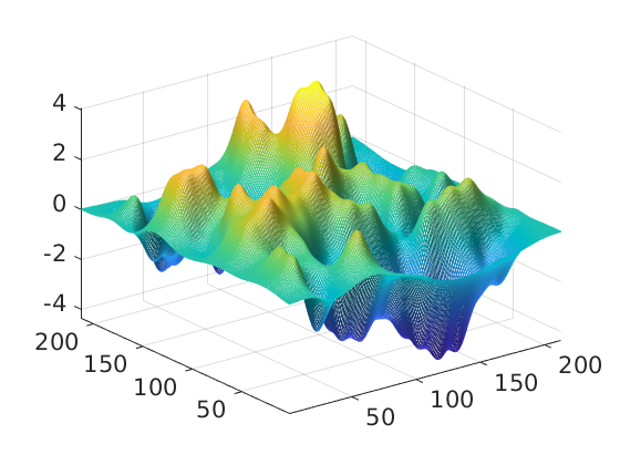
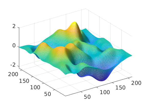
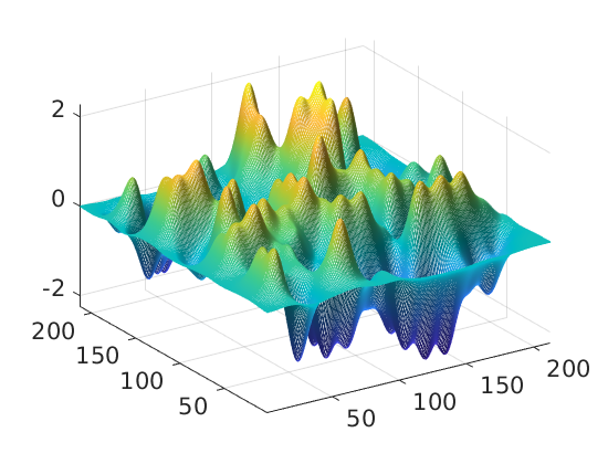
Figure 4.2: Full-, long- and short-range components of the multi-Slater tensor. Slater kernels with $\lambda=0.5$ and with random amplitudes in the range of $[-5,5]$ are placed in the nodes of a $12\times 12\times 4$ lattice using 3D grid of size $n^{\otimes 3}$ with $n=384$, $R=8,R_{l}=3$ and the number of nodes $N=576$.

Figure 4.3 and Table 4.2 demonstrate the decomposition of the multi-Slater tensor with the amplitudes in the nodes modulated by the function of the (x,y,z)-coordinates

$$F(x,y,z)=c_{1}\cos(x+2y+4z)\exp(-c_{2}\sqrt{x^{2}+2y^{2}+4z^{2}}),$$ (4.21)

with $c_{1}=6$ and $c_{2}=0.1$.

Next, we generate a tensor composed of a sum of discretized Slater functions on a sampling lattice $L_{1}\times L_{2}\times L_{3}$, living on 3D representation grid of size $n^{\otimes 3}$ with $n=232$. The amplitudes of the individual Slater functions are modulated by a function of $x,y,z$-coordinates (4.21) in every node of the lattice. Table 4.2 shows rank of the long-range part of this multi-Slater tensor with respect to the increasing size of the lattice. $N=L_{1}\,L_{2}\,L_{3}$ is the number of nodes, and $R_{ini}$ and $R_{comp}$ are the initial and compressed canonical ranks, respectively. Tucker ranks are shown at the canonical-to-Tucker decomposition step. Threshold values for the Slater potential generation is $\varepsilon_{N}=10^{-5}$, the thresholds for the canonical-to-canonical rank reduction procedure are given by $\varepsilon_{Tuck}=10^{-3}$ and $\varepsilon_{T2C}=10^{-5}$. Table 4.2 demonstrates the very moderate icrease of the reduced rank in the long-range part of the Slater potential sum on the size of the 3D sampling lattice.

$L_{1}\times L_{2}\times L_{3}$	$N$	Tucker ranks	$R_{ini}$	$R_{comp}$
$4\times 4\times 4$	64	$7\times 7\times 7$	256	25
$6\times 6\times 6$	216	$7\times 7\times 7$	648	23
$8\times 8\times 8$	512	$7\times 7\times 7$	1536	30
$16\times 16\times 8$	2048	$10\times 9\times 6$	6144	47
$16\times 16\times 16$	4096	$10\times 9\times 8$	12288	55

Table 4.2: Reduced canonical ranks for the case of functional amplitudes. $R_{L}=3$, $R_{L}=5$, $\varepsilon_{N}=10^{-5}$, $\varepsilon_{Tuck}=10^{-3}$, $\varepsilon_{T2C}=10^{-5}$.

Figure 4.3 demonstrates the full-, long- and short-range components of the multi-Slater tensor. Slater kernels with $\lambda=0.5$ and with the amplitudes modulated by the function (4.21) of the $(x,y,z)$-coordinates are places on the nodes of a $12\times 12\times 4$ sampling lattice, living on 3D grid of size $n^{\otimes 3}$ with $n=384$, $R=8,R_{l}=3$, and with the number of sampling nodes $N=576$.

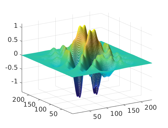
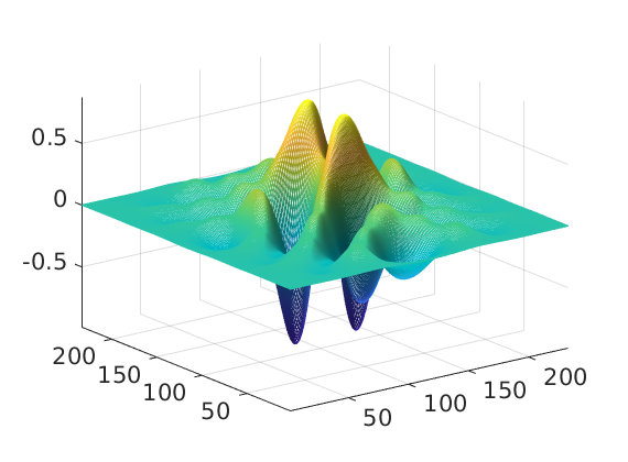
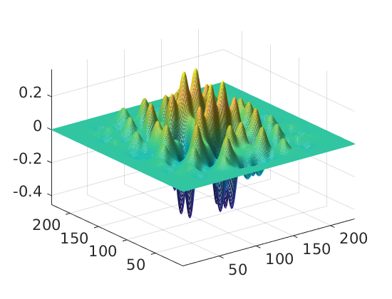
Figure 4.3: Full-, long- and short-range components of the multi-Slater tensor. Slater kernels with $\lambda=0.5$ and with amplitudes modulated by the function (4.21) using the nodes of a $12\times 12\times 4$ lattice on 3D grid of size $n^{\otimes 3}$ with $n=384$, $R=8,R_{l}=3$ and the number of nodes $N=576$.

5 Representing Green’s kernels in tensor format

In this section we demonstrate how the RHOSVD can be applied for the efficient tensor decomposition of various singular radial functions composed by polynomial expansions of a few reference potentials already precomputed in the low-rank tensor format. Given the low-rank CP tensor ${\bf A}$ further considered as a reference tensor, the low rank representation of the tensor-valued polynomial function

$${P}({\bf A})=a_{0}{\bf I}+a_{1}{\bf A}+a_{2}{\bf A}^{2}+\cdots+a_{n}{\bf A}^{n},$$

where the multiplication of tensors is understood in the sense of pointwise Hadamard product, can be calculated via $n$-times application of the RHOSVD by using the Horner scheme in the form

$$P(x)=a_{0}+x(a_{1}+x(a_{2}+x(a_{3}+\ldots x(a_{n-1}+a_{n}x)\ldots))).$$

Similar scheme can be also applied in the case of multivariate polynomials.

For examples considered in this section we make use of the discretized Slater $e^{-\|x\|}$ and Newton $\frac{1}{\|x\|}$, $x\in\mathbb{R}^{d}$, kernels as the reference tensors. The following statement was proven in [19, 29] (see also Lemma 4.4).

Proposition 5.1

The discretized over $n^{\otimes d}$-grid radial functions $e^{-\|x\|}$ and $\frac{1}{\|x\|}$, $x\in\mathbb{R}^{d}$, included in representation of various Green kernels and fundamental solutions for elliptic operators with constant coefficients, both allow the low-rank CP tensor approximation. The corresponding rank-$R$ representations can be calculated in $O(dRn)$ operations without precomputing and storage of the target tensor in the full (entry-wise) format.

Tensor decomposition for discretized singular kernels such as $\|x\|$, $\frac{1}{\|x\|^{m}}$, $m\geq 2$, and $e^{-\kappa\|x\|}/\|x\|$, can be now calculated by applying the RHOSVD to polynomial combinations of the reference potentials as in Proposition 5.1. The most important benefit of the presented techniques is the opportunity to compute the rank-$R$ tensor approximations without precomputing and storage of the target tensor in the full format tensor.

In what follows, we present the particular examples of singular kernels in $\mathbb{R}^{d}$ which can be treated by the above presented techniques. Consider the fundamental solution of the advection-diffusion operator ${\cal L}_{d}$ with constant coefficients in $\mathbb{R}^{d}$

$${\cal L}_{d}=-\Delta+2\bar{b}\cdot\nabla+\kappa^{2},\quad\bar{b}\in\mathbb{C}^{d},\quad\kappa\in\mathbb{C}.$$

If $\kappa^{2}+|\bar{b}|^{2}=0$, then for $d\geq 3$ it holds

$$\eta_{0}(x)=\frac{1}{(d-2)\omega_{d}}\frac{e^{\langle\bar{b},x\rangle}}{\|x\|^{d-2}},$$

where $\omega_{d}$ is the surface area of the unit sphere in $\mathbb{R}^{d}$. Notice that the radial function $\frac{1}{\|x\|^{d-2}}$ for $d\geq 3$ allows the RS decomposition of the corresponding discrete tensor representation based on the sinc quadrature approximation, which implies the RS representation of the kernel function $\eta_{0}(x)$, since the function $e^{\langle\bar{b},x\rangle}$ is already separable. From computational point of view, both the CP and RS canonical decompositions of discretized kernels $\frac{1}{\|x\|^{d-2}}$ can be computed by successive application of RHOSVD approximation to the products of canonical tensors for the discretized Newton potential $\frac{1}{\|x\|}$.

In the particular case $\bar{b}=0$, we obtain the fundamental solution of the operator ${\cal L}_{3}=-\Delta+\kappa^{2}$ for $d=3$, also known as the Yukawa (for $\kappa\in\mathbb{R}_{+}$) or Helmholtz (for $\kappa\in\mathbb{C}$) Green kernels

$$\eta_{\lambda}(x)=\frac{1}{4\pi}e^{-\kappa\|x\|}/\|x\|,\quad x\in\mathbb{R}^{3}.$$

In the case of Yukawa kernel the tensor representations by using Gaussian sums are considered in [59, 60], see also references therein.

The Helmholtz equation with $\mbox{Im}\,\kappa>0$ (corresponds to the diffraction potentials) arises in problems of acoustics, electro-magnetics and optics. We refer to [45] for the detailed discussion of this class of fundamental solutions. Fast algorithms for the oscillating Helmholtz kernel have been considered in [59]. However, in this case the construction of the RS tensor decomposition remains an open question.

In the case of 3D biharmonic operator ${\cal L}=\Delta^{2}$ the fundamental solution reads as

$$p(\|x\|)=-\frac{1}{8\pi}\|x\|,\quad x\in\mathbb{R}^{3}.$$

The hydrodynamic potentials correspond to the classical Stokes operator

$$\nu\Delta{u}-\mbox{grad}\,p={f},\quad\mbox{div}\,{u}=0,$$

where ${u}$ is the velocity field, $p$ denotes the pressure, and $\nu$ is the constant viscosity coefficient. The solution of the Stokes problem in $\mathbb{R}^{3}$ can be expressed by the hydrodynamic potentials

$$u_{k}(x)=\int\limits_{\mathbb{R}^{3}}\sum\limits^{3}_{\ell=1}\Psi_{k\ell}(x-{y})f_{\ell}({y})\mbox{d}{y},\quad p(x)=\int\limits_{\mathbb{R}^{3}}\langle\Theta(x-{y}),{f})({y})\rangle\mbox{d}{y}$$ (5.1)

with the fundamental solution

$$\Psi_{k\ell}(x)=\frac{1}{8\pi\nu}\left(\frac{\delta_{k\ell}}{\|x\|}+\frac{x_{k}x_{\ell}}{\|x\|^{3}}\right),\quad\Theta(x)=\frac{x}{4\pi\|x\|^{3}},\quad x\in\mathbb{R}^{3}.$$ (5.2)

The existence of the low-rank RS tensor representation for the hydrodynamic potential is based on the same argument as in Remark 5.1. In turn, in the case of biharmonic fundamental solution we use the identity

$$\|x\|=\frac{\|x\|^{2}}{\|x\|},$$

where the nominator has the separation rank equals to $d$. The latter representation can be also applied for calculation of the respective tensor approximations.

Here we demonstrate how the application of RHOSVD allows to easily compute the low rank Tucker/CP approximation of the discretized singular potential $\frac{1}{\|x\|^{3}}$, $x\in\mathbb{R}^{3}$, as well as the respective RS-representation, having at hand the RS representation of the tensor ${\bf P}\in\mathbb{R}^{n\otimes 3}$ discretizing the Newton kernel. In this example, we use the discretization of $\frac{1}{\|x\|^{3}}$ in the form

$${\bf P}^{(3)}={\bf P}\odot{\bf P}\odot{\bf P},$$

where by ${\bf P}^{(3)}$ we denotes the collocation projection discretization of $\frac{1}{\|x\|^{3}}$. The low rank Tucker/CP tensor approximation to ${\bf P}^{(3)}$ can be computed by the direct application of the RHOSVD to the above product type representation. The RS representation of ${\bf P}^{(3)}$ is calculated based on Lemma 4.3. Given the RS-representation (4.11) of the discretized Newton kernel, ${\bf P}_{R}$, we define the low rank CP approximation to the discretized singular part in the hydrodynamic potential ${\bf P}^{(3)}$ by

$${\bf P}^{(3)}_{R^{\prime}}={\bf P}_{R}\odot{\bf P}_{R}\odot{\bf P}_{R}.$$

In view of Lemma 4.3, the long range part of RS decomposition of ${\bf P}^{(3)}_{R^{\prime}}$, can be computed by RHOSVD approximation to the following Hadamard product of tensors,

$${\bf P}^{(3)}_{R^{\prime}_{l}}={\bf P}_{R_{l}}\odot{\bf P}_{R_{l}}\odot{\bf P}_{R_{l}}.$$

Figure 5.1 visualizes the tensor ${\bf P}^{(3)}_{R^{\prime}}$ as well as its long range part ${\bf P}^{(3)}_{R^{\prime}_{l}}$.

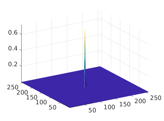
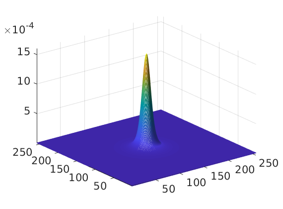
Figure 5.1: RHOSVD approximation of the discretized cubic potential $\frac{1}{\|x\|^{3}}$ and its long-range part.

The potentials are discretized on $n\times n\times n$ Cartesian grid with $n=257$, the rank truncation threshold is chosen for $\varepsilon=10^{-5}$. The CP rank of the Newton kernel is equal to $R=19$, while we set $R_{l}=10$, thus resulting in the initial ranks $6859$ and $10^{3}$ for RHOSVD decomposition of ${\bf P}^{(3)}_{R^{\prime}}$ and ${\bf P}^{(3)}_{R^{\prime}_{l}}$, respectively. The RHOSVD decomposition reduces the large rank parameters to $R^{\prime}=122$ (the Tucker rank is $r=13$) and ${R^{\prime}_{l}}=58$ (the Tucker rank is $r=8$), correspondingly.

6 RHOSVD for rank reduction in 3D elliptic problem solvers

Efficient rank reduction procedure based on the RHOSVD is a prerequisite for the development of the tensor-structured solvers for the three-dimensional elliptic problem, which reduce the computational complexity to almost linear scale, $O(nR)$, contrary to usual $O(n^{3})$ complexity.

Assume that all input data in the governing PDE are given in the low-rank tensor form. The convenient tensor format for these problems is a canonical tensor representation of both the governing operator, and of the initial guess as well as of the right hand side. The commonly used numerical techniques are based on certain iterative schemes that include at each iterative step multiple matrix-vector and vector-vector algebraic operations each of them enlarges the tensor rank of the output in the additive or multiplicative way. It turns out that in common practice the most computationally intensive step in the rank-structured algorithms is the adaptive rank truncation, which makes the rank truncation procedure ubiquitous.

We notice that in PDE based mathematical models the total numerical complexity of the particular computational scheme, i.e. the overall cost of the rank truncation procedure is determined by the multiple of the number of calls to the rank truncation algorithm (merely the number of iterations) and the cost of a single RHOSVD transform (mainly determined by the rank parameter of the input tensor). In turn, both complexity characteristics depend on the quality of the rank-structured preconditioner so that optimization of the whole solution process is can be achieved by the trade-off between Kronecker rank of the preconditioner and the complexity of its implementation.

In the course of preconditioned iterations, the tensor ranks of the governing operator, the preconditioner and the iterand are multiplied, and therefore a robust rank reduction is mandatory procedure for such techniques applied to iterative solution of elliptic and pseudo-differential equations in the rank-structured tensor format.

In particular, the RHOSVD was applied to the numerical solution of PDE constrained (including the case of fractional operators) optimal control problems [22, 53], where the complexity of the order $O(nR\log n)$ was demonstrated. In the case of higher dimensions the rank reduction in the canonical format can be performed directly (i.e., without intermediate use of the Tucker approximation) by using the cascading ALS iteration in the CP format, see [35] concerning the tensor-structured solution of the stochastic/parametric PDEs.

7 Conclusions

We discuss theoretical and computational aspects of the RHOSVD served for approximation of tensors in low-rank Tucker/canonical formats, and show that this rank reduction technique is the principal ingredient in tensor-based computations for real-life problems in scientific computing and data modeling. We recall rank reduction scheme for the canonical input tensors based on RHOSVD and subsequent Tucker-to-canonical transform. We present the detailed error analysis of low rank RHOSVD approximation to the canonical tensors (possibly with large input rank), and provide the proof on the uniform bound for the relative approximation error.

We recall that the first example on application of the RHOSVD was the rank-structured computation of the 3D convolution transform with the nonlocal Newton kernel in $\mathbb{R}^{3}$, which is the basic operation in the Hartree-Fock calculations.

The RHOSVD is the basic tools for utilizing the multilinear algebra in RS tensor format, which employs the sinc-analytic tensor approximation methods applied to the important class of radial functions in $\mathbb{R}^{d}$. This enables efficient rank decompositions of tensors generated by functions with multiple local cusps or singularities by separating their short- and long-range parts. As an example, we construct the RS tensor representation of the discretized Slater function $e^{-\lambda\|x\|}$, $x\in\mathbb{R}^{d}$. We then describe the RS tensor approximation to various Green’s kernels obtained by combination of this function with other potentials, in particular, with the Newton kernel providing the Yukawa potential. In this way, we introduce the concept of reproducing radial functions which pave the way for efficient RS tensor decomposition applied to a wide range of function-related multidimensional data by combining the multilinear algebra in RS tensor format with the RHOSDV rank reduction techniques.

Our next example is related to application of RHOSVD to low-rank tensor interpolation of scattered data. Our numerical tests demonstrate the efficiency of this approach on the example of multi-Slater interpolant in the case of many measurement points. We apply the RHOSVD to the data generated via random or function modulated amplitudes of samples and demonstrate numerically that for both cases the rank of the long-range part remains small and depends weakly on the number of samples.

Finally, we notice that the described RHOSVD algorithms have proven their efficiency in a number of recent applications, in particular, in rank reduction for the tensor-structured iterative solvers for PDE constraint optimal control problems (including fractional control), in construction of the range-separated tensor representations for calculation of the electrostatic potentials of many-particle systems (arising in protein modeling), and for numerical analysis of large scattered data in $\mathbb{R}^{d}$.

References

- [1] M. Abramowitz and I. A. Stegun. Handbook of Mathematical Functions. Dover Publ., New York, 1968.
- [2] M. Bachmayr, R. Schneider and A. Uschmajew. Tensor networks and hierarchical tensors for the solution of high-dimensional partial differential equations. Foundations of Computational Mathematics 16 (6), 1423-1472, 2016.
- [3] P. Benner, V. Khoromskaia and B. N. Khoromskij. Range-Separated Tensor Format for Many-Particle Modeling. SIAM J Sci. Comput., 40 (2), A1034-A1062, 2018.
- [4] P. Benner, V. Khoromskaia, B. N. Khoromskij, C. Kweyu and M. Stein. Regularization of Poisson–Boltzmann Type Equations with Singular Source Terms Using the Range-Separated Tensor Format. SIAM J. Sci. Comput., 43 (1), A415-A445, 2021.
- [5] T. Boiveau, V. Ehrlacher, A. Ern and A. Nouy. Low-rank approximation of linear parabolic equations by space-time tensor Galerkin methods. ESAIM: Mathematical Modelling and Numerical Analysis 53 (2), 635-658, 2019.
- [6] D. Braess. Nonlinear approximation theory. Springer-Verlag, Berlin, 1986.
- [7] A. Cichocki, N. Lee, I Oseledets, A. H. Pan, Q. Zhao and D. P. Mandic. Tensor networks for dimensionality reduction and large-scale optimization: Part 1 low-rank tensor decompositions. Foundations and Trends in Machine Learning 9 (4-5), 249-429, 2016.
- [8] P. Comon. Tensor decompositions. Mathematics in Signal Processing V, 1-24, 2002.
- [9] P. Comon, X. Luciani, A.L.F. De Almeida. Tensor decompositions, alternating least squares and other tales. Journal of Chemometrics: A Journal of the Chemometrics Society 23 (7‐8), 393-405, 2009.
- [10] L. De Lathauwer, B. De Moor, J. Vandewalle. A multilinear singular value decomposition. SIAM J. Matrix Anal. Appl., 21 (2000) 1253-1278.
- [11] S. Dolgov, D. Kalise and K. K. Kunisch. Tensor Decomposition Methods for High-dimensional Hamilton–Jacobi–Bellman Equations. SIAM J. Sci. Comput., 43 (3), A1625-A1650, 2021.
- [12] S. V. Dolgov, B. N. Khoromskij, and I. Oseledets. Fast solution of multi-dimensional parabolic problems in the TT/QTT formats with initial application to the Fokker-Planck equation. SIAM J. Sci. Comput., 34 (6), 2012, A3016-A3038.
- [13] S. Dolgov and J. W. Pearson. Preconditioners and tensor product solvers for optimal control problems from chemotaxis. SIAM J. Sci. Comput., 41 (6), B1228-B1253, 2019.
- [14] V. Ehrlacher, L. Grigori, D. Lombardi and H. Song. Adaptive hierarchical subtensor partitioning for tensor compression. SIAM J. Sci. Comput., 43 (1), A139-A163, 2021.
- [15] M. Espig, W. Hackbusch, A. Litvinenko, H. G. Matthies, E. Zander. Post-Processing of High-Dimensional Data. E-preprint arXiv:1906.05669, 2019.
- [16] G.H. Golub, C.F. Van Loan. Matrix Computations. Johns Hopkins University Press, Baltimore, MD, 1996.
- [17] L. Grasedyck. Hierarchical singular value decomposition of tensors. SIAM. J. Matrix Anal. & Appl 31, 2029, 2010.
- [18] W. Hackbusch and S. Kühn. A new scheme for the tensor representation. J. Fourier Anal. Appl. 15 (2009), no. 5, 706-722.
- [19] W. Hackbusch and B. N. Khoromskij. Low-rank Kronecker product approximation to multi-dimensional nonlocal operators. Part I. Separable approximation of multi-variate functions. Computing 76 (2006), 177-202.
- [20] W. Hackbusch and A. Uschmajew. Modified iterations for data-sparse solution of linear systems. Vietnam journal of mathematics, 49 (2021) 2, p. 493-512.
- [21] R. A. Harshman. Foundations of the PARAFAC procedure: Models and conditions for an “explanatory” multimodal factor analysis. UCLA Working Papers in Phonetics, 16, 1-84. (University Microfilms, Ann Arbor, Michigan, No. 10,085), (1970).
- [22] G. Heidel, V. Khoromskaia, B. N. Khoromskij and V. Schulz. Tensor product method for fast solution of optimal control problems with fractional multidimensional Laplacian in constraints. J Comput. Physics, 424, 109865, 2021.
- [23] F.L. Hitchcock. The expression of a tensor or a polyadic as a sum of products. J. Math. Physics, 6 (1927), 164-189.
- [24] G. C. Hsiao, and W. L. Wendland. Boundary integral equations. Springer, Berlin (2008).
- [25] V. Kazeev, M. Khammash, M. Nip, and Ch. Schwab. Direct Solution of the Chemical Master Equation Using Quantized Tensor Trains. PLoS Comput Biol 10(3), 2014.
- [26] V. Khoromskaia. Numerical Solution of the Hartree-Fock Equation by Multilevel Tensor-structured methods. TU Berlin, 2010. https://depositonce.tu-berlin.de/handle/11303/3016
- [27] V. Khoromskaia, B. N. Khoromskij. Grid-based Lattice Summation of Electrostatic Potentials by Assembled Rank-structured Tensor Approximation. Comp. Phys. Comm., 185, 2014, pp. 3162-3174.
- [28] V. Khoromskaia and B. N. Khoromskij. Prospects of Tensor-Based Numerical Modeling of the Collective Electrostatics in Many-Particle Systems. Computational Mathematics and Mathematical Physics 61 (5), 864-886, 2021.
- [29] B. N. Khoromskij. Structured Rank- Decomposition of Function-related Tensors in . Comp. Meth. Applied Math., 6, (2006), 2, 194-220.
- [30] B. N. Khoromskij. -Quantics Approximation of - Tensors in High-Dimensional Numerical Modeling. Constructive Approximation, v.34(2), 2011, 257-289.
- [31] B. N. Khoromskij. Range-separated tensor decomposition of the discretized Dirac delta and elliptic operator inverse. J. Comp. Physics, v. 401, 108998, 2020.
- [32] B. N. Khoromskij and V. Khoromskaia. Low Rank Tucker-Type Tensor Approximation to Classical Potentials. Central European J. of Math., 5(3), pp.523-550, 2007.
- [33] B. N. Khoromskij and V. Khoromskaia. Multigrid Tensor Approximation of Function Related Arrays. SIAM J. Sci. Comp., 31(4), 3002-3026 (2009).
- [34] B.N. Khoromskij, V. Khoromskaia, and H.-J. Flad. Numerical Solution of the Hartree-Fock Equation in Multilevel Tensor-structured Format. SIAM J. Sci. Comp. 33(1) (2011) 45-65.
- [35] B. N. Khoromskij and C. Schwab. Tensor-structured Galerkin approximation of parametric and stochastic elliptic PDEs. SIAM J. Sci. Comput., 33 (1), 364-385, 2011.
- [36] D. Kressner, M. Steinlechner, and A. Uschmajew. Low-rank tensor methods with subspace correction for symmetric eigenvalue problems. SIAM J Sci. Comp., 36 (5), A2346-A2368, 2014.
- [37] D. Kressner and A. Uschmajew. On low-rank approximability of solutions to high-dimensional operator equations and eigenvalue problems. Lin. Algebra Appl., 493, 556-572, 2016.
- [38] C. Kweyu, V. Khoromskaia, B. Khoromskij, M. Stein and P. Benner. Solution decomposition for the nonlinear Poisson-Boltzmann equation using the range-separated tensor format. arXiv preprint arXiv:2109.14073, 2021.
- [39] E.B. Lindgren, A. J. Stace, E. Polack, Y. Maday, B. Stamm and E. Besley. An integral equation approach to calculate electrostatic interactions in many-body dielectric systems. J. Comp. Phys., 371, 2018, pp.712-731.
- [40] A. Litvinenko, D. Keyes, V. Khoromskaia, B. N. Khoromskij and H. G. Matthies. Tucker tensor analysis of Matern functions in spatial statistics. Comput. Meth. Appl. Math., 2019, 19(1) pp.101-122.
- [41] A. Litvinenko, Y. Marzouk, H. G. Matthies, M. Scavino, A. Spantini. Computing f-Divergences and Distances of High-Dimensional Probability Density Functions–Low-Rank Tensor Approximations. E-preprint arXiv:2111.07164, 2021.
- [42] Ch. Lubich, T. Rohwedder, R. Schneider and B. Vandereycken. Dynamical approximation of hierarchical Tucker and tensor-train tensors. SIAM J Matrix Anal. Appl., 34 (2), 470-494, 2013.
- [43] B. Matérn. Spatial Variation, vol. 36 of Lecture Notes in Statistics, Springer-Verlag, Berlin; New York, second edition ed., 1986.
- [44] C. Marcati, M. Rakhuba and C. Schwab. Tensor Rank bounds for Point Singularities in . E-preprint arXiv:1912.07996, 2019.
- [45] V. Maz’ya, G. Schmidt. Approximate Approximations, Math. Surveys and Monographs, vol. 141, AMS 2007.
- [46] I. V. Oseledets. Tensor-train decomposition. SIAM J. Sci. Comp., 33(5), pp. 2295-2317, 2011.
- [47] I. V. Oseledets, M. V. Rakhuba and A. Uschmajew. Alternating least squares as moving subspace correction. SIAM Journal on Numerical Analysis 56 (6), 3459-3479, 2018.
- [48] I. Oseledets and E. E. Tyrtyshnikov. TT-cross approximation for multidimensional arrays. Linear Algebra Appl. 432 (2010), no.1, 70-88.
- [49] I. V. Oseledets, and E. E. Tyrtyshnikov, Breaking the Curse of Dimensionality, or How to Use SVD in Many Dimensions. SIAM J. Sci. Comp., v. 31(5) (2009), 3744-3759.
- [50] M. Rakhuba and I. Oseledets. Fast multidimensional convolution in low-rank tensor formats via cross approximation. SIAM J Sci. Comp., 37 (2), A565-A582, 2015.
- [51] S. A. Sauter and Ch. Schwab. Boundary Element Methods. Springer, 2011.
- [52] A. Smilde, R. Bro, and P. Geladi. Multi-way analysis with applications in the chemical sciences. Wiley, 2004.
- [53] B. Schmitt, B. N. Khoromskij, V. Khoromskaia and V. Schulz. Tensor method for optimal control problems constrained by fractional three-dimensional elliptic operator with variable coefficients. Numer. Linear Algebra Appl., 2021, 1-24, e2404.
- [54] N. D. Sidiropoulos, L. De Lathauwer, X. Fu, K. Huang, E. E Papalexakis, Ch. Faloutsos. Tensor decomposition for signal processing and machine learning. IEEE Transactions on Signal Processing 65 (13), 3551-3582, 2017.
- [55] F. Stenger. Numerical methods based on Sinc and analytic functions. Springer-Verlag, 1993.
- [56] J. M. F. Ten Berge, N. D. Sidiropoulos. On uniqueness in CANDECOMP/PARAFAC. Psychometrika 67 (3), 399-409, 2002.
- [57] L. R. Tucker. Some mathematical notes on three-mode factor analysis. Psychometrika, 31 (1966) 279-311.
- [58] A. Uschmajew. Local convergence of the alternating least squares algorithm for canonical tensor approximation. SIAM J. Matr. Anal. Appl., 33 (2), 639-652, 2012.
- [59] B. N. Khoromskij. Tensor Numerical Methods in Scientific Computing. De Gruyter Verlag, Berlin, 2018.
- [60] V. Khoromskaia and B. N. Khoromskij. Tensor numerical methods in quantum chemistry. De Gruyter Verlag, Berlin, 2018.