Deep Learning based Multi-User Power Allocation and Hybrid Precoding in Massive MIMO Systems

Abstract

This paper proposes a deep learning based power allocation (DL-PA) and hybrid precoding technique for multi-user massive multiple-input multiple-output (MU-mMIMO) systems. We first utilize an angular-based hybrid precoding technique for reducing the number of RF chains and channel estimation overhead. Then, we develop the DL-PA algorithm via a fully-connected deep neural network (DNN). DL-PA has two phases: (i) offline supervised learning with the optimal allocated powers obtained by particle swarm optimization based PA (PSO-PA) algorithm, (ii) online power prediction by the trained DNN. In comparison to the computationally expensive PSO-PA, it is shown that DL-PA greatly reduces the runtime by $98.6\%$-$99.9\%$, while closely achieving the optimal sum-rate capacity. It makes DL-PA a promising algorithm for the real-time online applications in MU-mMIMO systems.

I Introduction

Millimeter wave (mmWave) has been considered as a promising candidate for the fifth-generation (5G) and beyond for its large available bandwidth [1]. Also, its shorter wavelengths are appealing for massive multiple-input multiple-output (mMIMO) technology since it enables the implementation of large antenna arrays in relatively smaller physical dimensions [2]. On the other hand, mMIMO technology alleviates the severe path loss effect in mmWave communications via high beamforming gain.

For multi-user downlink transmission, the conventional MIMO systems generally consider the single-stage fully-digital precoding (FDP) [3]. However, FDP causes two major challenges for multi-user mMIMO (MU-mMIMO) systems: (i) the high hardware cost/complexity with the requirement of one dedicated power-hungry radio frequency (RF) chain per each antenna, (ii) large channel estimation overhead size [4]. Alternatively, two-stage hybrid precoding (HP) interconnects the digital baseband(BB)-stage and analog RF-stage with significantly reduced number of RF chains[5, 6, 7]. Also, an angular-based HP (AB-HP) technique is developed in [8], where analog RF-stage via is designed the slow time-varying angle-of-departure (AoD) information. Thus, AB-HP addresses both aforementioned challenges by decreasing the channel estimation overhead and the number of RF chains. On the other hand, multi-user power allocation (PA) is a non-convex optimization problem due to the effect of inter-user interference [9]. Recently, [10] proposes an iterative particle swarm intelligence based PA (PSO-PA) algorithm for maximizing the overall system capacity in MU-mMIMO systems. Although it is shown that PSO-PA achieves the globally optimal system capacity, it requires longer runtime as the optimization space (i.e., number of users) increases.

As a key driving force for artificial intelligence (AI), deep learning has been successfully applied in many fields including computer vision, speech recognition and natural language processing [11]. Hence, the success of deep learning also motivates its applications in wireless communication systems [12, 13, 14]. For instance, deep learning has been applied for signal detection [12], resource management [13], channel estimation [14]. Our ultimate goal is to investigate deep learning for a low-complexity PA technique achieving near-optimal system capacity with acceptable runtime considering real-time applications in MU-mMIMO systems with HP.

In this paper, we propose a novel low-complexity deep learning based PA (DL-PA) algorithm in MU-mMIMO systems utilizing HP architecture. We first employ AB-HP for the downlink transmission to reduce the number of RF chains and the channel estimation overhead size. Then, the proposed DL-PA is built via a fully-connected deep neural network (DNN). There are two phases in DL-PA: (i) offline supervised learning via the optimal allocated powers calculated with PSO-PA, (ii) online power prediction via the trained DNN. Numerical results present that DL-PA nearly achieves the optimal sum-rate capacity calculated by PSO-PA (e.g., $96.5\%$-$99.7\%$ of optimal capacity). Also, the runtime of PSO-PA is remarkably reduced by $98.6\%$-$99.9\%$ via DL-PA, which is essential regarding the real-time online applications.

The rest of this paper is organized as follows. Section II expresses the system model. Section III introduces AB-HP. Section IV presents the proposed DL-PA. After the illustrative results in Section V, the paper is concluded in Section VI.

II System Model

A single-cell MU-mMIMO system is modeled for the downlink transmission as illustrated in Fig. 1. Here, the base station (BS) is equipped with a uniform rectangular array (URA) having $M=M_{x}\times M_{y}$ antennas to serve $K$ single-antenna user equipments (UEs) clustered in $G$ groups.

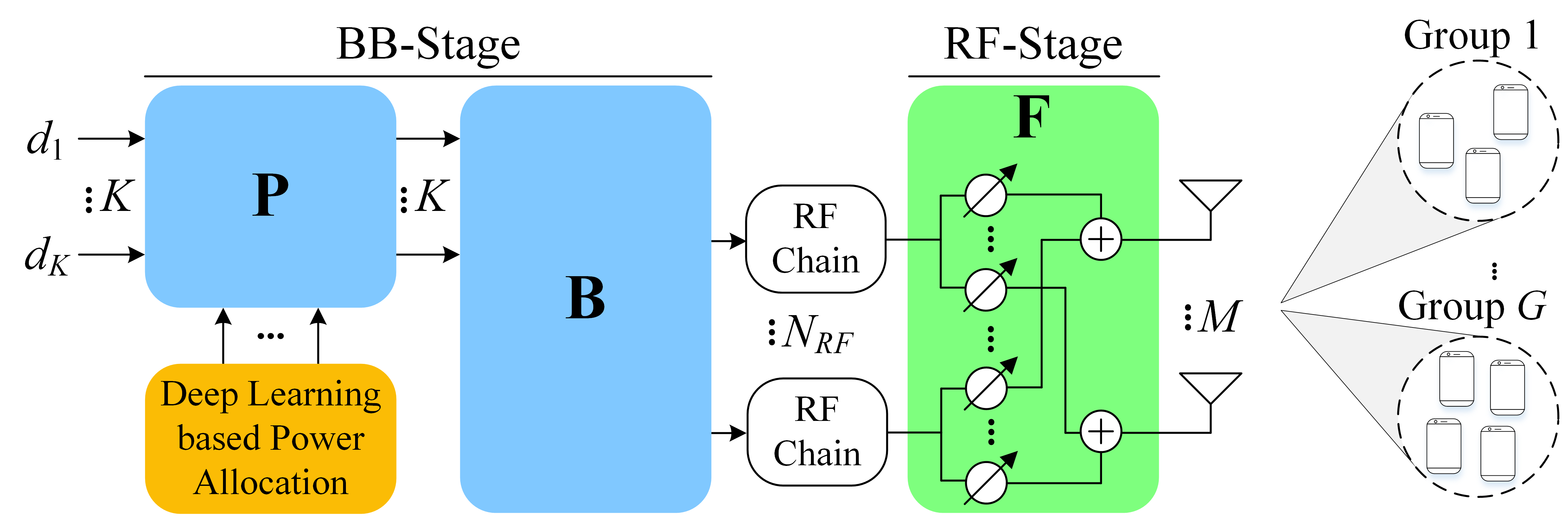
Figure 1: Massive MIMO system with hybrid precoding.

As presented in Fig. 1, the RF-stage and BB-stage are interconnected via $N_{RF}$ RF chains to reduce the hardware cost/complexity (i.e., $K\leq N_{RF}\ll M$). First, the analog RF beamformer ${\bf F}\in\mathbb{C}^{M\times N_{RF}}$ is developed via the low-cost phase-shifters for the RF-stage. Second, the digital BB precoder ${\bf B}=\left[{\bf b}_{1},\cdots,{\bf b}_{K}\right]\in\mathbb{C}^{N_{RF}\times K}$ and the multi-user PA matrix ${\bf P}=\textrm{diag}\left(\sqrt{p_{1}},\cdots,\sqrt{p_{K}}\right)\in\mathbb{R}^{K\times K}$ are constructed for the BB-stage, where ${\bf b}_{k}\in\mathbb{C}^{N_{RF}}$ and $p_{k}$ are the BB precoder vector and the non-negative allocated power for the $k^{th}$ UE, respectively. Hence, the transmitted downlink vector is defined as ${\bf s}={\bf FBPd}\in\mathbb{C}^{M}$, where ${\bf d}=\left[d_{1},\cdots,d_{K}\right]\in\mathbb{C}^{K}$ is the data signal vector with $\mathbb{E}\big{\{}{\bf dd}^{H}\big{\}}={\bf I}_{K}$. It is important to mention that ${\bf s}\in\mathbb{C}^{M}$ satisfies the total transmit power constraint of $P_{T}$ (i.e., $\mathbb{E}\big{\{}\big{\|}{\bf s}\big{\|}^{2}_{2}\big{\}}\leq P_{T}$).

According to the 3D geometry-based mmWave channel model [1] and the URA structure [8], the channel vector for the $k^{th}$ UE is defined as follows:

$${\bf{h}}_{k}^{T}=\sum_{l=1}^{Q}\tau^{-\eta}_{k_{l}}z_{k_{l}}{\bm{\phi}}^{T}\big{(}{{\gamma_{x,k_{l}}},{\gamma_{y,k_{l}}}}\big{)}={\bf{z}}^{T}_{k}{{\bf{\Phi}}}_{k}\in\mathbb{C}^{M},$$ (1)

where $Q$ is the number of paths, $\tau_{k_{l}}$ and $z_{k_{l}}\sim\mathcal{CN}\big{(}0,{1}/{Q}\big{)}$ are respectively the distance and complex path gain of $l^{th}$ path, $\eta$ is the path loss exponent, ${\bm{\phi}}\big{(}\cdot,\cdot\big{)}\in\mathbb{C}^{M}$ is the phase response vector, $\gamma_{x,k_{l}}=\sin\left(\theta_{k_{l}}\right)\cos\left(\psi_{k_{l}}\right)$ and $\gamma_{y,k_{l}}=\sin\left(\theta_{k_{l}}\right)\sin\left(\psi_{k_{l}}\right)$ are the coefficients reflecting the elevation AoD (EAoD) and azimuth AoD (AAoD) for the corresponding path. Here, $\theta_{k_{l}}\in\big{[}\theta_{k}-\delta_{k}^{\theta},\theta_{k}+\delta_{k}^{\theta}\big{]}$ is the EAoD with mean $\theta_{k}$ and spread $\delta_{k}^{\theta}$, $\psi_{k_{l}}\in\big{[}\psi_{k}-\delta_{k}^{\psi},\psi_{k}+\delta_{k}^{\psi}\big{]}$ is the AAoD with mean $\psi_{k}$ and spread $\delta_{k}^{\psi}$. Then, the phase response vector is modeled as [8]:

$${\bm{\phi}}\left({{\gamma_{x},\gamma_{y}}}\right) =\big{[}{1,{e^{-j2\pi d{{\gamma_{x}}}}},\cdots,{e^{-j2\pi d\left({{M_{x}}-1}\right){{\gamma_{x}}}}}}\big{]}^{T}$$ (2)

$$\otimes\big{[}{1,{e^{-j2\pi d{{\gamma_{y}}}}},\cdots,{e^{-j2\pi d\left({{M_{y}}-1}\right){{\gamma_{y}}}}}}\big{]}^{T}\in\mathbb{C}^{M},$$

where $d$ is the antenna spacing normalized by wavelength. The instantaneous channel vector expressed in (1) is a function of the fast time-varying path gain vector ${\bf z}_{k}=\big{[}\tau^{-\eta}_{k_{1}}z_{k_{1}},\cdots,\tau^{-\eta}_{k_{Q}}z_{k_{Q}}\big{]}^{T}\in\mathbb{C}^{Q}$ and slow time-varying phase response matrix ${{\bf{\Phi}}}_{k}\in\mathbb{C}^{Q\times M}$ based on AoD information.

Afterwards, the received signal at the $k^{th}$ UE is written as:

$$r_{k} ={\bf h}_{k}^{T}{\bf s}+n_{k}={\bf h}_{k}^{T}{\bf FBPd}+n_{k}$$ (3)

$$=\underbrace{\sqrt{p_{k}}{\bf h}_{k}^{T}{\bf Fb}_{k}d_{k}}_{\textrm{Desired Signal}}+\underbrace{\sum\nolimits_{t\neq k}^{K}\sqrt{p_{t}}{\bf h}_{k}^{T}{\bf Fb}_{t}d_{t}}_{\textrm{Inter UE Interference}}+n_{k},$$

where $n_{k}\sim\mathcal{CN}\big{(}0,\sigma_{n}^{2}\big{)}$ is the circularly symmetric complex Gaussian noise. After some mathematical manipulations, we derive the instantaneous signal-to-interference-plus-noise-ratio (SINR) at the $k^{th}$ UE as follows:

$$\textrm{SINR}_{k}\left({\bf F},{\bf B},{\bf P}\right)=\frac{p_{k}\left|{\bf h}_{k}^{T}{\bf Fb}_{k}\right|^{2}}{\sum_{t\neq k}^{K}p_{t}\left|{\bf h}_{k}^{T}{\bf Fb}_{t}\right|^{2}+\sigma_{n}^{2}}.$$ (4)

Then, the ergodic sum-rate capacity is calculated as $R_{\textrm{sum}}=\mathbb{E}\big{\{}\sum_{k=1}^{K}\log_{2}\big{[}1+\textrm{SINR}_{k}\left({\bf F},{\bf B},{\bf P}\right)\big{]}\big{\}}$. For maximizing the system capacity, we formulate the optimization problem as:

$$\max_{{\bf F},{\bf B},{\bf P}}{} \sum_{k=1}^{K}\log_{2}\left(1+\frac{p_{k}\left|{\bf h}_{k}^{T}{\bf Fb}_{k}\right|^{2}}{\sum_{t\neq k}^{K}p_{t}\left|{\bf h}_{k}^{T}{\bf Fb}_{t}\right|^{2}+\sigma_{n}^{2}}\right)$$ (5)

s.t. $$C_{1}:\mathbb{E}\big{\{}\left\|{\bf{s}}\right\|^{2}_{2}\big{\}}=\sum_{k=1}^{K}{{p_{k}}{\bf{b}}_{k}^{H}{{\bf{F}}^{H}}{\bf{F}}{{\bf{b}}_{k}}}\leq{P_{T}},$$

$$C_{2}:p_{k}\geq 0,\forall k,$$

$$C_{3}:\big{|}\left[{\bf{F}}\right]_{i,j}\big{|}=\frac{1}{\sqrt{M}},\forall i,j,$$

where $C_{1}$ and $C_{2}$ indicate the total and per UE transmit power constraints, respectively, $C_{3}$ refers to the constant modulus (CM) constraint due to the utilization of phase-shifters at the RF-stage. However, it is a non-convex optimization because of two reasons: (i) the allocated powers entangled with each other [9], (ii) the CM constraint at the analog RF beamformer [5]. Thus, we sequentially design the hybrid precoding architecture illustrated in Fig. 1. First, the analog RF beamformer and the digital BB precoder are designed based on AB-HP technique in Section III, then the multi-user PA matrix is developed via the proposed deep learning based PA (DL-PA) algorithm in Section IV.

III Angular-Based Hybrid Precoding (AB-HP)

Throughout this section, our ultimate goals are to (i) reduce the number of RF chains, (ii) decrease the channel estimation overhead, (iii) mitigate the inter UE interference via AB-HP technique for MU-mMIMO systems.

III-A Analog RF Beamformer

We construct the analog RF beamformer by focusing the signal energy in the desired direction via the slow-time varying AoD information. By using (1) and assuming the users clustered in the same groups experience similar AoDs [14], the channel matrix for group $g$ is given by:

$${\bf H}_{g}=\big{[}{\bf h}_{g_{1}},\cdots,{\bf h}_{g_{K_{g}}}\big{]}^{T}={\bf Z}_{g}{\bf\Phi}_{g}\in\mathbb{C}^{K_{g}\times M},$$ (6)

where $g_{k}=k+\sum_{t=1}^{g-1}K_{t}$ is the UE index with $K=\sum_{g=1}^{G}K_{g}$, ${\bf Z}_{g}=\big{[}{\bf z}_{g_{1}},\cdots,{\bf z}_{g_{K_{g}}}\big{]}^{T}\in\mathbb{C}^{K_{g}\times Q}$ is the fast time-varying path gain matrix, ${\bf\Phi}_{g}\in\mathbb{C}^{Q\times M}$ is the slow time-varying phase response matrix. Afterwards, the concatenated full-size channel matrix is defined as ${\bf H}=\left[{\bf H}_{1}^{T},\cdots,{\bf H}_{G}^{T}\right]^{T}\in\mathbb{C}^{K\times M}$.

Then, $G$ blocks are designed for the RF beamformer as:

$${\bf F}=\left[{\bf F}_{1},\cdots,{\bf F}_{G}\right]\in\mathbb{C}^{M\times N_{RF}},$$ (7)

where ${\bf F}_{g}\in\mathbb{C}^{M\times N_{RF,g}}$ is the RF beamformer for group $g$ with $N_{RF}=\sum\nolimits_{g=1}^{G}N_{RF,g}$. By using (6) and (7), the effective channel matrix seen from the BB-stage is obtained as:

$$\tilde{\bf{H}}={\bf H}{\bf F}=\left[{\begin{array}[]{*{20}{c}}{{{\bf{H}}_{1}}{{\bf{F}}_{1}}}&{{{\bf{H}}_{1}}{{\bf{F}}_{2}}}&{\cdots}&{{{\bf{H}}_{1}}{{\bf{F}}_{G}}}\\ {{{\bf{H}}_{2}}{{\bf{F}}_{1}}}&{{{\bf{H}}_{2}}{{\bf{F}}_{2}}}&{\cdots}&{{{\bf{H}}_{2}}{{\bf{F}}_{G}}}\\ {\vdots}&{\vdots}&{\ddots}&{\vdots}\\ {{{\bf{H}}_{G}}{{\bf{F}}_{1}}}&{{{\bf{H}}_{G}}{{\bf{F}}_{2}}}&{\cdots}&{{{\bf{H}}_{G}}{{\bf{F}}_{G}}}\\ \end{array}}\right]\in\mathbb{C}^{K\times N_{RF}},$$ (8)

where ${\bf H}_{g}{\bf F}_{g}={\bf Z}_{g}{\bf\Phi}_{g}{\bf F}_{g}\in\mathbb{C}^{K_{g}\times N_{RF,g}}$ is the effective channel matrix for group $g$ and ${\bf H}_{t}{\bf F}_{g}={\bf Z}_{t}{\bf\Phi}_{t}{\bf F}_{g}\in\mathbb{C}^{K_{t}\times N_{RF,g}}$ is the effective interference channel matrix, $\forall t\neq g$.

Hence, the RF beamformer design targets accomplishing the following two objectives: (i) maximizing the beamforming gain in the desired direction (i.e., $\textrm{Span}\left({\bf F}_{g}\right)\subset\textrm{Span}\left({\bf\Phi}_{g}\right)$), (ii) successfully suppress the interference among UE groups (i.e., $\textrm{Span}\left({\bf F}_{g}\right)\subset\cup_{t\neq g}\textrm{Null}\left({\bf\Phi}_{t}\right)$). As proven in [8], both objectives are accomplished by building the RF beamformer ${\bf F}_{g}$ via the steering vector ${\bf e}\left(\gamma_{x},\gamma_{y}\right)=\frac{1}{\sqrt{M}}{\bm{\phi}}^{*}\left({{\gamma_{x},\gamma_{y}}}\right)\in\mathbb{C}^{M}$ with $\left(\gamma_{x},\gamma_{y}\right)$ angle-pairs covering the AoD support of desired UE group and excluding the AoD supports of the other UE groups (please see (2) for ${\bm{\phi}}\left({{\gamma_{x},\gamma_{y}}}\right)$). For covering the complete 3D elevation and azimuth angular space with minimum number of angle-pairs, $M$ orthogonal quantized angle-pairs are defined as ${{\lambda^{x}_{u}}=-1+\frac{2u-1}{{{M_{x}}}}}$ for $u=1,\cdots,{M_{x}}$ and ${{\lambda^{y}_{c}}=-1+\frac{2c-1}{{{M_{y}}}}}$ for $c=1,\cdots,{M_{y}}$. Considering that $N_{RF,g}$ quantized angle-pairs covers the AoD support of group $g$ [8, eq. (13)], we build the RF beamformer for UE group $g$ as follows:

$${\bf F}_{g}=\big{[}{\bf e}\big{(}\lambda_{u_{1}}^{x},\lambda_{c_{1}}^{y}\big{)},\cdots,{\bf e}\big{(}\lambda_{u_{N_{RF,g}}}^{x},\lambda_{c_{N_{RF,g}}}^{y}\big{)}\big{]}\in\mathbb{C}^{M\times N_{RF,g}}.$$ (9)

Finally, the complete RF beamformer ${\bf F}$ satisfying the CM constraint (i.e., $C_{3}$ given in (5)) is derived by substituting (9) into (7). It is worthwhile to mention that the analog RF beamformer is a unitary matrix (i.e., ${\bf F}^{H}{\bf F}={\bf I}_{N_{RF}}$).

III-B Digital BB Precoder

We aim to further mitigate the residual inter UE interference at the digital BB precoder. Thus, the regularized zero-forcing (RZF) technique is applied via joint group processing [8]. By utilizing the reduced-size effective channel matrix $\tilde{\bf{H}}$ defined in (8), the digital BB precoder is constructed as [3]:

$${\bf B}=\left[\tilde{\bf{H}}^{H}\tilde{\bf{H}}+K\frac{\sigma_{n}^{2}}{P_{T}}{\bf I}_{N_{RF}}\right]^{-1}\tilde{\bf{H}}^{H}\in\mathbb{C}^{N_{RF}\times K}.$$ (10)

IV A Low-Complexity Deep Learning based
Power Allocation

After developing the analog RF beamformer $\bf F$ and the digital BB precoder $\bf B$, the capacity maximization optimization problem given in (5) is reformulated as follows:

$$\max_{{\bf P}}{} \sum_{k=1}^{K}\log_{2}\left(1+\frac{p_{k}\left|{\bf h}_{k}^{T}{\bf Fb}_{k}\right|^{2}}{\sum_{t\neq k}^{K}p_{t}\left|{\bf h}_{k}^{T}{\bf Fb}_{t}\right|^{2}+\sigma_{n}^{2}}\right)$$ (11)

s.t. $$C_{1}:\mathbb{E}\big{\{}\left\|{\bf{s}}\right\|^{2}_{2}\big{\}}=\sum_{k=1}^{K}{{p_{k}}{\bf{b}}_{k}^{H}{{\bf{F}}^{H}}{\bf{F}}{{\bf{b}}_{k}}}\leq{P_{T}},$$

$$C_{2}:p_{k}\geq 0,\forall k,$$

However, it is still a non-convex optimization problem due to the optimization variables as ${\bf P}=\textrm{diag}\left(\sqrt{p}_{1},\cdots,\sqrt{p}_{K}\right)$ interchangeably located in the numerator and denominator [9]. Thus, the traditional optimization algorithms may not be utilized to solve the PA problem.

Recently, a particle swarm optimization based power allocation (PSO-PA) technique for finding the optimal allocated powers is proposed in [10]. In comparison to the computationally expensive exhaustive search, it is numerically shown that the global optimal solution is achieved via PSO-PA. However, as the number of UEs increases (i.e., higher dimensional optimization space), PSO-PA requires more iterations and longer runtime. Thus, the enhanced computational complexity might make PSO-PA impractical for the real-time online applications of MU-mMIMO systems.

For achieving a near-optimal sum-rate performance while keeping a reasonable runtime, we propose a low-complexity deep learning based power allocation (DL-PA) algorithm. Here, we have two phases as demonstrated in Fig. 2: (i) Phase 1 applies the offline supervised learning via the optimal allocated power values calculated by PSO-PA, (ii) Phase 2 runs the trained DL-PA algorithm for predicting the allocated powers in the real-time online applications.

Hence, the reminder of this section introduces the DNN architecture, loss functions, dataset generation and training process for the proposed low-complexity DL-PA algorithm.

IV-A Deep Neural Network Architecture

We model a fully-connected deep neural network (DNN) architecture with three hidden layers as illustrated in Fig. 3, which aims to predict the optimal allocated powers for $K$ downlink UEs. There are $L_{i}$ neurons present at the $i^{th}$ hidden layer with $i=1,2,3$. On the other hand, as shown in Fig. 2, the effective channel matrix $\tilde{\bf H}={\bf HF}=\big{[}\tilde{\bf h}_{1}^{T},\cdots,\tilde{\bf h}_{K}^{T}\big{]}\in\mathbb{C}^{K\times N_{RF}}$ given in (8) and the digital BB precoder ${\bf B}=\big{[}{\bf b}_{1},\cdots,{\bf b}_{K}\big{]}\in\mathbb{C}^{N_{RF}\times K}$ given in (10) are employed as inputs in the proposed DL-PA algorithm. The input feature scaling and vectorization operations are applied to $\tilde{\bf H}$ and ${\bf B}$. Then, the input layer feature vector is obtained as:

$${\bf x}_{0}=\left[\begin{array}[]{*{20}{l}}\alpha_{1}{\bf x}_{\tilde{\bf h}_{1}}\\ \hskip 12.91663pt\vdots\\ \alpha_{1}{\bf x}_{\tilde{\bf h}_{K}}\\ \alpha_{2}{\bf x}_{{\bf b}_{1}}\\ \hskip 12.91663pt\vdots\\ \alpha_{2}{\bf x}_{{\bf b}_{K}}\\ \alpha_{3}{\bf{x}}_{\textrm{BB}}\\ \alpha_{4}{\bf{x}}_{\textrm{BB,inv}}\end{array}\right]\in\mathbb{R}^{L_{0}},$$ (12)

where $L_{0}=\left(4N_{RF}+2\right)K$ is the input feature size, ${\bf x}_{\tilde{\bf h}_{k}}=\big{[}\operatorname{Re}\big{(}\tilde{\bf{h}}_{k}^{T}\big{)},\operatorname{Im}\big{(}\tilde{\bf{h}}_{k}^{T}\big{)}\big{]}^{T}\in\mathbb{R}^{2N_{RF}}$, ${\bf x}_{{\bf b}_{k}}=\big{[}\operatorname{Re}\big{(}{\bf{b}}_{k}^{T}\big{)},\operatorname{Im}\big{(}{\bf{b}}_{k}^{T}\big{)}\big{]}^{T}\in\mathbb{R}^{2N_{RF}}$, ${\bf{x}}_{\textrm{BB}}^{T}=\big{[}{{\bf b}_{1}^{H}{\bf b}_{1}},\cdots,{{\bf b}_{K}^{H}{\bf b}_{K}}\big{]}^{T}\in\mathbb{R}^{K}$ and ${\bf{x}}_{\textrm{BB,inv}}^{T}=\big{[}\frac{1}{{\bf b}_{1}^{H}{\bf b}_{1}},\cdots,\frac{1}{{\bf b}_{K}^{H}{\bf b}_{K}}\big{]}^{T}\in\mathbb{R}^{K}$ are respectively the non-scaled input feature vectors for the effective channel, BB precoder, the gain of each BB precoder vector and its inverse. By implementing the maximum absolute scaling [16], the corresponding scaling coefficients are calculated as:

$$\alpha_{1} =\max\left(\big{|}{\bf x}_{\tilde{\bf h}_{1}}^{T}\big{|},\cdots,\big{|}{\bf x}_{\tilde{\bf h}_{K}}^{T}\big{|}\right)^{-1}$$ (13)

$$\alpha_{2} =\max\left(\big{|}{\bf x}_{{\bf b}_{1}}^{T}\big{|},\cdots,\big{|}{\bf x}_{{\bf b}_{K}}^{T}\big{|}\right)^{-1}$$

$$\alpha_{3} =\max\left({{\bf b}_{1}^{H}{\bf b}_{1}},\cdots,{{\bf b}_{K}^{H}{\bf b}_{K}}\right)^{-1}$$

$$\alpha_{4} =\min\left({{\bf b}_{1}^{H}{\bf b}_{1}},\cdots,{{\bf b}_{K}^{H}{\bf b}_{K}}\right).$$

Hence, each element of the input feature vector is scaled between $-1$ and $1$ (i.e., ${\bf x}_{0}\in\left[-1,1\right]$) by the maximum absolute scaling technique. It prevents the domination of large valued features on the small valued features [16].

In the offline supervised learning process (i.e., Phase 1), the optimal allocated powers are calculated as the output labels via the computationally expensive PSO-PA algorithm. Similar to the input features, we also apply the maximum absolute scaling to the optimal allocated powers as follows:

$$\bar{p}_{k}=\frac{p_{k}^{\textrm{opt}}}{\max\left({p_{1}^{\textrm{opt}}},\cdots,{p_{K}^{\textrm{opt}}}\right)}\in\left[0,1\right].$$ (14)

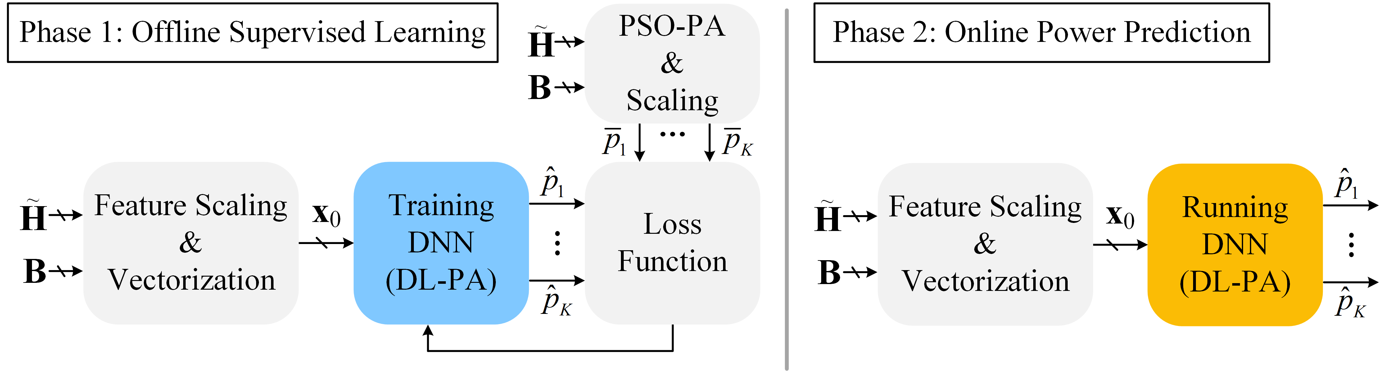
Figure 2: Block diagram of offline supervised learning (Phase 1) and online power prediction (Phase 2) in the DL-PA algorithm.

For the non-linear operations, we utilize the rectified linear unit (ReLU) as the activation function at the hidden layers (i.e., $f_{r}\left(x\right)=\max\left(0,x\right)$ [11]). Therefore, by using the input feature vector ${\bf x}_{0}$ given in (12), the output of $i^{th}$ hidden layer is calculated as ${{\bf x}_{i}=f_{r}\left({\bf W}_{i-1}{\bf x}_{i-1}+{\bf b}_{i-1}\right)\in\mathbb{R}^{L_{i}}}$, where ${\bf W}_{i-1}\in\mathbb{R}^{L_{i}\times L_{i-1}}$ and ${\bf b}_{i-1}\in\mathbb{R}^{L_{i}}$ are the weight matrix and bias vector, respectively. In order to fit the output layer predictions between $0$ and $1$ as in the output labels expressed in (14), we employ the sigmoid function at the output layer (i.e., $f_{\sigma}\left(x\right)=\frac{1}{1+e^{-x}}$ [11]). Thus, the predicted power values for $K$ downlink UEs via the DNN architecture are written as:

$$\left[\right. \hskip 3.22916pt\left.\hat{p}_{1},\hat{p}_{2},\cdots,\hat{p}_{K}\right]$$ (15)

$$=f_{\sigma}\left({\bf W}_{3}{\bf x}_{3}+{\bf b}_{3}\right)$$

$$=f_{\sigma}\left({\bf W}_{3}f_{r}\left({\bf W}_{2}f_{r}\left({\bf W}_{1}f_{r}\left({\bf W}_{0}{\bf x}_{0}+{\bf b}_{0}\right)+{\bf b}_{1}\right)+{\bf b}_{2}\right)+{\bf b}_{3}\right).$$

By using (10) and (15), we finally derive the multi-user PA matrix satisfying the transmit power constraint of $P_{T}$ as:

$${\bf P}=\sqrt{\frac{P_{T}}{\sum\nolimits_{k=1}^{K}\hat{p}_{k}{\bf b}_{k}^{H}{\bf b}_{k}}}\textrm{diag}\left(\sqrt{\hat{p}_{1}},\sqrt{\hat{p}_{2}},\cdots,\sqrt{\hat{p}_{K}}\right).$$ (16)

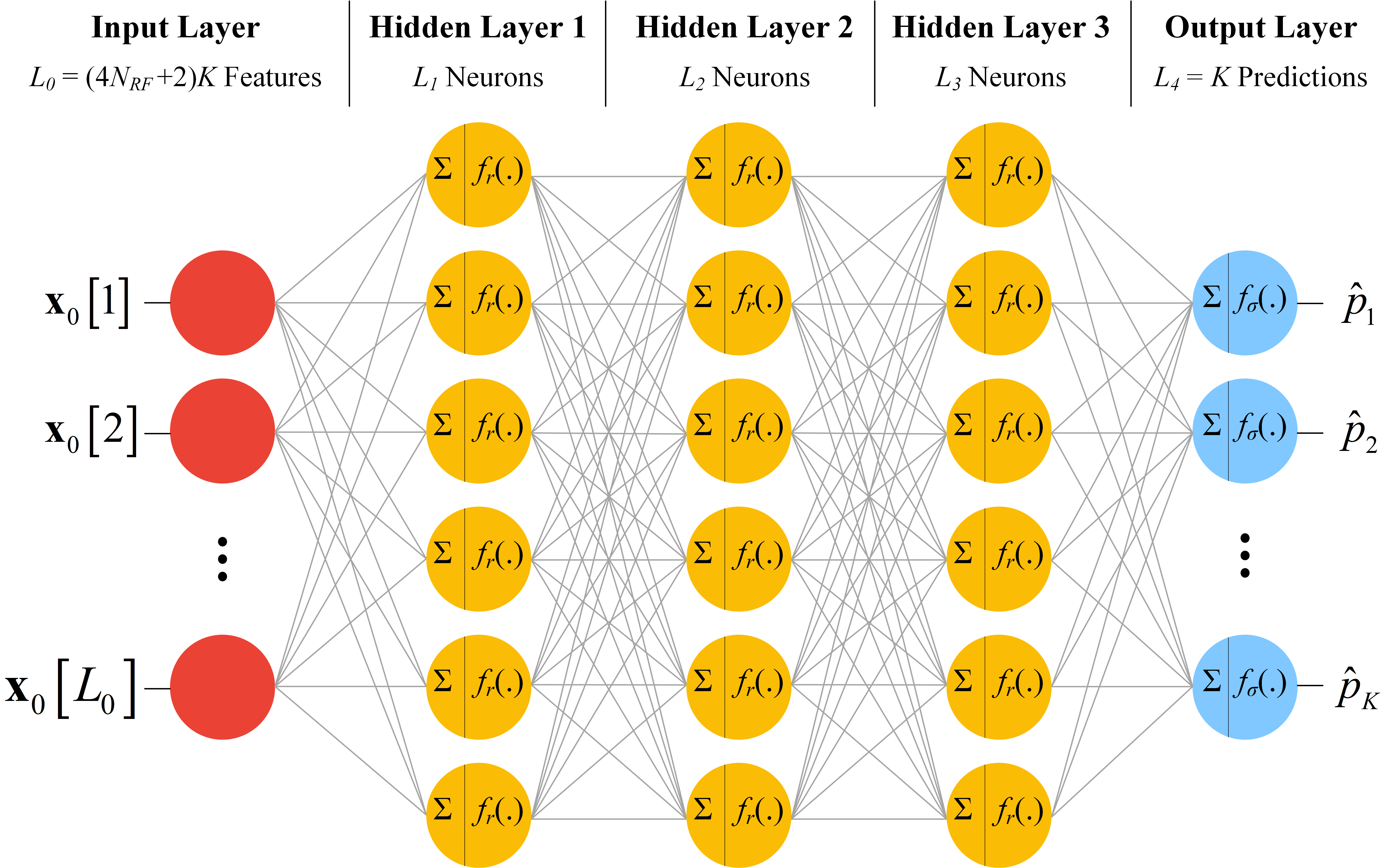
Figure 3: Deep neural network architecture for DL-PA algorithm.

IV-B Loss Functions

We here consider two loss functions by using the predicted and optimal power values: (i) mean square error (MSE), (ii) mean absolute error (MAE). When there are $S$ network realizations in the dataset, the MSE loss function is given by:

$$\mathcal{L}_{\textrm{MSE}} =\frac{1}{SK}\sum_{i=1}^{S}\sum_{{k=1}}^{K}\left(\bar{p}_{k,i}-\hat{p}_{k,i}\right)^{2}.$$ (17)

Similarly, the MAE loss function is written as:

$$\mathcal{L}_{\textrm{MAE}} =\frac{1}{SK}\sum_{i=1}^{S}\sum_{{k=1}}^{K}\left|\bar{p}_{k,i}-\hat{p}_{k,i}\right|.$$ (18)

By back-propagating the gradients of loss function from the output layer to the input layer, the weight matrices ${\bf W}_{i}$ and bias vectors ${\bf b}_{i}$ are updated for reducing the loss and closely predicting the optimal allocated power values. Hence, we ultimately optimize the sum-rate capacity of MU-mMIMO systems as expressed in (11).

IV-C Dataset Generation & Training Process

We generate a dataset with $S=100.000=10^{5}$ network realizations for the offline supervised learning process (i.e., Phase 1) illustrated in Fig. 2. In each realization, the channel vector expressed in (1) is generated for each UE by randomly varying the path gains, AoD parameters and UE location with respect to the BS. The corresponding optimal allocated powers are calculated via the PSO-PA algorithm [10, Algorithm 1] and stored in the dataset. For the offline learning process, we always consider $80\%$-$20\%$ split of the total available dataset among the training and validation.After completing the offline learning process (i.e., Phase 1), the online power allocation (i.e., Phase 2) is tested with a purely new test dataset. The DNN architecture for the proposed DL-PA algorithm is implemented using the open-source deep learning libraries in TensorFlow [17].

V Illustrative Results

This section presents sum-rate and runtime results for evaluating the proposed AB-HP with deep learning based power allocation (DL-PA) in the MU-mMIMO systems. The simulation parameters according to the 3D microcell scenario are summarized in Table I. Furthermore, the hyper-parameters for the DNN architecture are outlined in Table II.

TABLE I: Simulation parameters.

Number of antennas [18]	$M=16\times 16=256$
BS transmit power [18]	$P_{T}=20$ dBm
Cell radius [18]	100m
BS height [18] —. UE height [18]	10m —. 1.5m-2.5m
UE-BS horizontal distance	10m – 90m
UE groups	$G=1$ or $G=2$
UE per group	$K_{g}=\frac{K}{G}$
Mean EAoD —. Mean AAoD	$\theta_{g}=60^{\circ}$ —. $\psi_{g}=21^{\circ}+180^{\circ}\left(g-1\right)$
EAoD spread —. AAoD spread	$\delta_{g}^{\theta}=15^{\circ}$ —. $\delta_{g}^{\psi}=11^{\circ}$
Path loss exponent [19]	$\eta=3.76$
Noise PSD [19]	$-174$ dBm/Hz
Channel bandwidth [19]	$10$ kHz
# of paths[18]	$Q=20$
Antenna spacing (in wavelength)	${d=0.5}$

TABLE II: DNN hyper-parameters.

$1^{th}$ hidden layer size	$L_{1}=1024$
$2^{th}$ hidden layer size	$L_{2}=512$
$3^{th}$ hidden layer size	$L_{3}=256$
Dataset size	$S=100.000$
Test dataset size	$1.000$
Epoch size —. Batch size	$25$ —. $32$
Learning rate	$0.001$
Optimizer	ADAM [17]

Fig. 4 plots the sum-rate of the proposed DL-PA with MSE and MAE loss functions defined in (17) and (18), respectively. Here, we provide the performance evaluation on training, validation and test dataset for $K=3$ and $K=6$ UEs in $G=1$ group. As a benchmark, DL-PA is compared with PSO-PA [10] and equal PA (EQ-PA). Numerical results reveal that the proposed DL-PA closely approaches PSO-PA in all training, validation and test. For instance, when there are $K=3$ UEs, DL-PA provides $44.6$ bps/Hz sum-rate capacity on test data and achieves $99.1\%$ of the optimal sum-rate capacity achieved by PSO-PA as $45$ bps/Hz. Additionally, the capacity is improved by approximately $25\%$ with respect to EQ-PA (i.e., from $35.7$ bps to $44.6$ bps/Hz). Moreover, when there are a larger number of UEs as $K=6$, the sum-rate improvement compared to EQ-PA increases $48.8\%$ on the test data (i.e., from $47.4$ bps to $70.1$ bps/Hz). However, as the number of UEs increases, the optimization space enlarges and we observe a slight decay in the test data performance. To illustrate, for $K=6$ UEs, DL-PA with MAE accomplishes $98.9\%$ of the optimal sum-rate performance on training data, which marginally drops to $98.1\%$ on the test data.

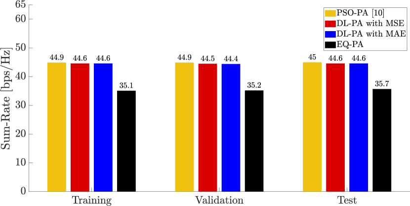
(a) $K=3$

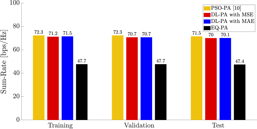
(b) $K=6$

Figure 4: Sum-rate performance evaluation on training, validation and test dataset ($G=1$ group).

In Fig. 5, the sum-rate performance is demonstrated versus the dataset size $S$, where there are either $K=3$ or $K=6$ UEs in $G=1$ group and dataset size varies between $500$ and $100.000$. It is seen that as the dataset size increases the gap between PSO-PA and DL-PA vanishes. As expected, the larger dataset size makes DL-PA learn better the optimal allocated powers, especially on the unseen test dataset.

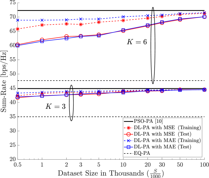
Figure 5: Sum-rate performance versus dataset size ($G=1$ group).

Fig. 6 displays both sum-rate and runtime results versus the number of UEs, which are equally clustered in $G=2$ groups (i.e., $K_{g}=\frac{K}{2}$).

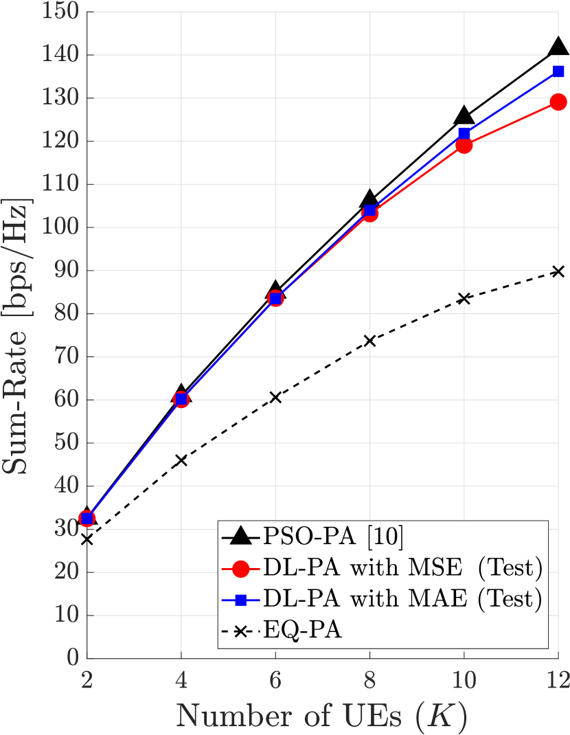
(a) Sum-rate

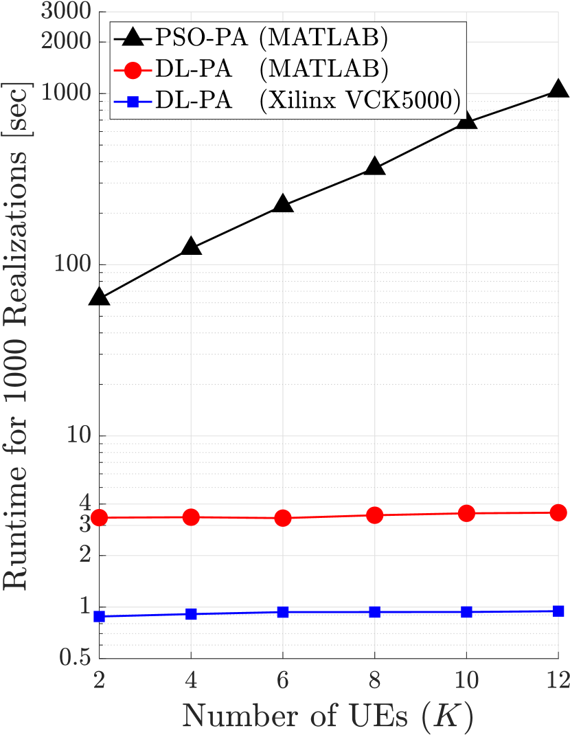
(b) Runtime

Figure 6: Sum-rate and runtime performance ($G=2$ groups).

As seen from Fig. 6(a), DL-PA with MAE outperforms its MSE counterpart as the number of UEs increases, although their performance difference is not distinguishable for a smaller number of UEs. On the other hand, the relative sum-rate performance of DL-PA with MAE compared to the optimal PSO-PA algorithm varies between $99.7\%$ and $96.5\%$ as shown in Table III. Moreover, the runtime comparison between PSO-PA and DL-PA is demonstrated for 1000 network realizations in Fig. 6(b). It is worthwhile to note that the offline trained DNN architecture for DL-PA algorithm is run on both MATLAB and Xilinx VCK5000 development card for AI inference [20]. We observe that the proposed DL-PA strikingly outperforms the computational complex PSO-PA algorithm by significantly reducing the runtime. To illustrate, when there are $K=12$ UEs, PSO-PA requires $1036.6$ sec, whereas only $0.9$ sec runtime is enough to run DL-PA on Xilinx VCK5000. Also, the runtime for DL-PA remains almost constant across all UE scenarios because the hidden layers have the same architecture for various UE cases (e.g., approximately $3.5$ sec on MATLAB and $0.9$ sec on Xilinx VCK5000). Thus, the runtime per realization is below 1 msec on Xilinx VCK5000. However, when there are more UEs, the runtime for PSO-PA exponentially increases due to the larger optimization space, where PSO-PA requires more iterations with the aim of finding the global optimal sum-rate. As presented in Table III, the relative runtime of DL-PA with MAE is reduced by $98.6\%$ for $K=2$ ($99.9\%$ for $K=12$) in comparison to the computationally expensive PSO-PA.

VI Conclusions

In this work, a novel deep learning based power allocation (DL-PA) and hybrid precoding technique has been proposed for maximizing sum-rate capacity in the MU-mMIMO systems. First, the angular-based hybrid precoding (AB-HP) scheme has been expressed for the downlink transmission to reduce the number of RF chains and lower the channel estimation overhead. Then, we have proposed the low-complexity DL-PA algorithm for predicting the optimal allocated power resources among the downlink UEs. The promising numerical results show that the proposed DL-PA closely approaches the optimal sum-rate capacity achieved by PSO-PA. On the other hand, DL-PA greatly reduces the runtime by $98.6\%$-$99.9\%$. It makes the implementation of DL-PA feasible for the real-time online applications in MU-mMIMO systems.

TABLE III: Relative performance of DL-PA with MAE ($G=2$).

	$K=2$	$K=4$	$K=6$	$K=8$	$K=10$	$K=12$
Sum-Rate	$99.7\%$	$98.7\%$	$98.3\%$	$98.0\%$	$97.1\%$	$96.5\%$
Runtime	$1.39\%$	$0.73\%$	$0.42\%$	$0.26\%$	$0.14\%$	$0.09\%$

References

• [1] A. N. Uwaechia et al., “A comprehensive survey on millimeter wave communications for fifth-generation wireless networks: Feasibility and challenges,” IEEE Access, vol. 8, pp. 62 367–62 414, 2020.
• [2] M. Agiwal et al., “Next generation 5G wireless networks: A comprehensive survey,” IEEE Commun. Surveys Tuts., vol. 18, no. 3, pp. 1617–1655, 3rd Quart. 2016.
• [3] N. Fatema et al., “Massive MIMO linear precoding: A survey,” IEEE Syst. J., vol. 12, no. 4, pp. 3920–3931, Dec. 2017.
• [4] A. F. Molisch et al., “Hybrid beamforming for massive MIMO: A survey,” IEEE Commun. Mag., vol. 55, no. 9, pp. 134–141, Sept. 2017.
• [5] I. Ahmed et al., “A survey on hybrid beamforming techniques in 5G: Architecture and system model perspectives,” IEEE Commun. Surveys Tuts., vol. 20, no. 4, pp. 3060–3097, 4th Quart. 2018.
• [6] A. Koc et al., “Full-duplex mmWave massive MIMO systems: A joint hybrid precoding/combining and self-interference cancellation design,” IEEE Open J. Commun. Soc., vol. 2, pp. 754–774, 2021.
• [7] M. Mahmood et al., “Energy-efficient MU-Massive-MIMO hybrid precoder design: Low-resolution phase shifters and digital-to-analog converters for 2D antenna array structures,” IEEE Open J. Commun. Soc., vol. 2, pp. 1842–1861, 2021.
• [8] A. Koc et al., “3D angular-based hybrid precoding and user grouping for uniform rectangular arrays in massive MU-MIMO systems,” IEEE Access, vol. 8, pp. 84 689–84 712, May 2020.
• [9] E. Björnson et al., “Optimal multiuser transmit beamforming: A difficult problem with a simple solution structure [lecture notes],” IEEE Signal Process. Mag., vol. 31, no. 4, pp. 142–148, 2014.
• [10] A. Koc et al., “Swarm intelligence based power allocation in hybrid massive MIMO systems,” in 2021 IEEE Wireless Commun. and Netw. Conf. (WCNC), Mar. 2021, pp. 1–7.
• [11] Y. LeCun et al., “Deep learning,” Nature, vol. 521, no. 7553, pp. 436–444, 2015.
• [12] H. Huang et al., “Deep learning for physical-layer 5G wireless techniques: Opportunities, challenges and solutions,” IEEE Wireless Commun., vol. 27, no. 1, pp. 214–222, 2020.
• [13] Y. Sun et al., “Application of machine learning in wireless networks: Key techniques and open issues,” IEEE Commun. Surveys Tuts., vol. 21, no. 4, pp. 3072–3108, 2019.
• [14] X. Zhu et al., “A deep learning and geospatial data based channel estimation technique for hybrid massive MIMO systems,” IEEE Access, vol. 9, pp. 145 115–145 132, 2021.
• [15] X.-S. Yang, Nature-inspired optimization algorithms.   Elsevier, 2014.
• [16] S. Galli, Python Feature Engineering Cookbook.   Packt Publishing Ltd, 2020.
• [17] M. Abadi et al., “Tensorflow: A system for large-scale machine learning,” in 12th USENIX Symp. Operating Syst. Design Implementation (OSDI 16), 2016, pp. 265–283.
• [18] 3GPP TR 38.901, “5G: Study on channel model for frequencies from 0.5 to 100 GHz,” Tech. Rep. Ver. 16.1.0, Nov. 2020.
• [19] 3GPP TR 36.931, “LTE; evolved universal terrestrial radio access (E-UTRA); radio frequency (RF) requirements for LTE pico node B,” Tech. Rep. Ver. 16.0.0, July 2020.
• [20] “VCK5000 Versal Development Card for AI Inference,” https://www.xilinx.com/products/boards-and-kits/vck5000.html, 2021, [Online; Accessed on Oct. 23, 2021].