Force Correlator for Driven Disordered Systems at Finite Temperature
Abstract
When driving a disordered elastic manifold through quenched disorder, the pinning forces exerted on the center of mass are fluctuating, with mean and variance , where is the externally imposed control parameter for the preferred position of the center of mass. was obtained via the functional renormalization group in the limit of vanishing temperature , and vanishing driving velocity . There are two fixed points, and deformations thereof, which are well understood: The depinning fixed point ( before ) rounded at , and the zero-temperature equilibrium fixed point ( before ) rounded at . Here we consider the whole parameter space of driving velocity and temperature , and quantify numerically the crossover between these two fixed points.
I Introduction
I.1 Generalities
Elastic manifolds driven in a disordered medium have a depinning transition at zero temperature. Typical examples are the motion of domain walls in magnets [1, 2, 3, 4], contact line depinning [5], earthquakes [6, 7] and the peeling of a RNA-DNA helix [8]. What these systems have in common is that they are governed by an over-damped equation of motion for the interface which is driven through a quenched disordered medium,
The disorder forces are short-range correlated, quenched random variables, whereas is a thermal noise. Their correlations are
| (2) | |||||
| (3) |
The equation of motion (I.1) can be studied via field theory. Its principle object is the renormalised force correlator . Interestingly, is the zero-velocity limit of the connected correlation function of the forces acting on the center of mass [9]
| (4) | |||||
The functional renormalization group (FRG) predicts two distinct universality classes, termed depinning and equilibrium. Equilibrium is the limit of first and then , whereas depinning is the limit of first and then . In both classes, has a cusp, and admits a scaling form
| (5) |
The characteristic sale scales with ,
| (6) |
defining a roughness exponent , distinct between depinning and equilibrium. A second difference is in the shape of .
The function was measured in numerical simulations [10, 11], and experiments [5, 2, 4, 12, 13]. These measurements, both in simulations and experiments, are done by moving the center of the confining potential of strength at a small driving velocity . For depinning, experiments were performed in soft ferro magnets, both with SR and LR elasticity [4] and DNA/RNA peeling [8]. An experiment in equilibrium is DNA unzipping [13]. In all cases, the measured force correlator agrees with the predictions from field theory and exactly solved models. It is rounded at a finite driving velocity. While the experiments above are for zero-temperature depinning, in general the finite driving velocity is not the only perturbation taking us away from the critical point (5): thermal noise at temperature in Eq. (I.1) has to be dealt with. Apart from the two fixed points depinning and equilibrium, also small deformations of these fixed points are well understood: For depinning, driving at a finite velocity can be accounted for by twice convoluting the zero-velocity fixed point with the response function, which leads to a rounding of the cuspy fixed point [14]. On the other hand, the equilibrium fixed point is rounded by a finite temperature, described by a boundary layer [15, 16]. The goal of this paper is to describe the crossover between these two limiting cases. We do this by means of numerical simulations. At fixed , our results are parametrised by and .
I.2 Mean-field description
Since these questions are difficult to treat numerically for an interface, our study is done for a single degree of freedom which can itself be interpreted as the center-of-mass of the interface, or the mean field. Denoting the center of mass of the interface by , the equation of motion (I.1) and noise correlations (2)-(3) reduce to
| (7) | |||||
| (8) | |||||
| (9) |
The first term is the force exerted by a confining well, which gets replaced by a Hookean spring with spring constant . is the random pinning force, possibly the derivative of a potential, . Specifying the correlations of defines the system. Following [14] we consider forces that describe an Ornstein-Uhlenbeck (OU) process driven by a Gaussian white noise
| (10) | |||||
At small distances , the forces have the statistics of a random walk, thus its microscopic limit is the ABBM model [17, 18]. At large distances forces are uncorrelated, putting our model in the random-field (RF) universality class.
Returning to the equation of motion (7), at zero temperature and at slow driving, most of the time the l.h.s. vanishes. This condition defines the force , given , and the associated critical force as
| (11) | |||||
| (12) |
The signs are such that exerting a positive force overcomes the pinning forces . Due to the thermal noise, can increase even below the threshold force by thermal activation over energy barriers . For sufficiently small velocities, this allows the dynamics to equilibrate with activation times following an Arrhenius law . Thermal fluctuations allow for to go backward, violating the Middleton theorem [19] (forward-only motion at ).
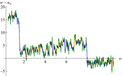
Fig. 1 shows one simulation, with the original trajectory which includes all noise in green. Smoothening it over time allows us to show predominantly forward movement in blue and backward movement in orange. We see that at this temperature backward movement is substantial.
The effective disorder is defined as
| (13) |
We have written subscripts to indicate that measurements depend on both and . Finally, the critical force is related to the area of the hysteresis loop as
| (14) |
Hysteresis is absent in equilibrium where and maximal at depinning.
I.3 Review of known results
Before we present our findings for the questions posed in the introduction, let us review what is known for a single perturbation.
I.3.1 Equilibrium fixed point
Subfigures (b) and (c): For , (b) and (c) comparison of the equilibrium (green, EM) to at (blue solid, DNS) and (orange solid, DNS). In dashed cyan/red, we show the combination (34). This correctly captures the amplitude, but a signal of anti-correlations remains. In the inset we show the difference , which quantifies the corrections due to non-equilibration.
The zero-temperature equilibrium fixed point can be measured by energy minimisation (EM) at fixed of
| (15) |
see appendix A for implementation details. The random potential is given by . For the random-field (RF) disorder relevant for Eq. (10), the model is known as the Sinai model, introduced in [20]. The effective force correlator reads (see [21], with corrections in [16])
| (16) | |||||
| (17) |
| (18) | ||||
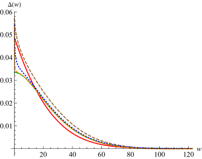
The roughness exponent is identified from Eq. (17) as . Fig. 2 shows in blue the analytical solution of Eqs. (16)-(18). In red and cyan are numerical simulations of Eq. (15) for uncorrelated forces, constant in an interval of size one, and unit variance, i.e. . Already for , the simulation has converged to the theory. The inset shows comparison to the model of OU forces defined in (10), which belongs to the same universality class.
At a finite temperature, thermal fluctuations smoothen the shocks and round the cusp in a boundary layer . This thermal rounding is shown in Fig. 3. The size of the boundary layer can be estimated from the FRG [16] (see appendix B)
| (19) | |||||
| (20) | |||||
| (21) |
The amplitude ensures normalisation, i.e. that the area under is preserved in the presence of thermal rounding. Since from (20) one sees that , the RHS of (20) is dimensionless. This defines the dimensionless temperature , scaling with its own exponent
| (22) |
is called the equilibrium energy exponent As we show in appendix B, an alternative expression for the boundary layer is given by
| (23) | |||||
| (24) | |||||
| (25) |
where is a diffusion kernel. A delicate question is what the dynamical exponent is in equilibrium. The observation that in both the free theory as well as at depinning suggests that this likely holds also in equilibrium. Finally, the pinning force in equilibrium.
I.3.2 Depinning fixed point
For depinning the effective disorder (4) is given by [22, 14]
| (26) | |||||
| (27) | |||||
| (28) |
The roughness exponent is ; the dynamical exponent is [14]. In the simulations, we can measure (26) at zero velocity, by moving the parabola from and waiting for the dynamics to cede. In an experiment, performed at finite , is rounded by the driving velocity [14]
| (29) |
By construction, and the integral of is independent of . At small , Eq. (29) can be approximated by
| (30) |
where is chosen s.t. .
II Results in the general situation
We now present our numerical results, mostly obtained by direct numerical simulation (DNS). First in section II.1 we check Eqs. (16)-(21) for equilibrium. In section II.2 we discuss several order parameters characterizing the crossover between equilibrium and depinning. Section II.3 shows that with the rescalings established so far, we can collapse all our data.
II.1 Thermal peak in the equilibrium regime
In Fig. 5 we show the results of numerical simulations of in the near-equilibrium regime. The presence of the thermal noise leads to a thermal peak (TP) at small . In absence of disorder it reads
| (32) | |||||
Here is the response function of the free theory. This is checked in Fig. 4(a).
Let us now turn back to the disordered case, at finite velocity and finite temperature . We make the ansatz
| (33) |
The first term is the relevant result for . The second term is the contribution (32) from the thermal noise. If the driving velocity is small enough for the dynamics to equilibrate, then we expect the third term to vanish, or at least to be small.
Figs. 4(b)-(c) show the combination
| (34) |
for (b) and (c). While correctly subtracts the thermal noise at , the remaining term is visible. In the inset, we show , i.e. the error we make in the approximation . We see that despite a difference of by a factor of ten, the rescaled combination at small depends little on . This estimates the boundary layer in our example to be .
II.2 Order parameters
II.2.1 The mean force as an order parameter
The measured pinning force
| (36) |
is maximal for depinning at temperature zero, and vanishes in equilibrium. It is a natural candidate for an order parameter. We define
| (37) |
which vanishes in equilibrium and is at depinning. The inset of Fig. 6 shows this force ratio for different and , for , and . Using that the dimensionless temperature is and velocity and temperature are related by Arrhenius’ law as , a natural ansatz for a scaling parameter is
| (38) |
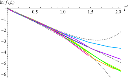
This collapses all curves on a single master curve, as shown in the main plot of Fig. 6. We can go one step further. To do so, let us plot the log of as a function of . We find on Fig. 7 an almost linear behaviour for an exponent , with slope . Thus
| (39) |
is a stretched exponential. Note that if the fit is attempted close to , one can also conclude on . If we restrict to 10 percent deviation, this allows for in the range . We expect the regime to be governed by the depinning fixed point, and by the equilibrium fixed point. The crossover regime should be best visible for .

II.2.2 The correlation length as an order parameter
In section II.2.1 we established the mean force as an order parameter between equilibrium and depinning. While this is the most robust quantity we found, there are other quantities one might use. The first is the correlation length , which decreases with temperature compared to its value at depinning. In all of the following, we will denote by the value at depinning, and by the finite-temperature value. If one considers zero-temperature depinning as a reference point, then at small temperatures
| (40) |
with , see Fig. 8.
II.2.3 The disorder amplitude as an order parameter
Assuming that
| (41) |
the amplitude at small should behave as
| (42) |
Our measurements presented in the inset of Fig. 9 are consistent with an exponent in the range .
II.2.4 The disorder integral as an order parameter
Both the correlation length as well as the amplitude are very sensitive to details of the rounding around the cusp. More robust is to consider the area under . The above relations above would imply that
| (43) |
Our data are consistent with an exponent in the range of to , favoring the upper end. The decrease of the area is shown in Fig. 9. The orange dashed lines are references for depinning (top) and equilibrium (bottom).
II.3 Scaling close to equilibrium and depinning
Let us next consider scaling close to equilibrium and depinning.
II.3.1 Scaling near equilibrium
For equilibrium
| (44) |
While this scaling holds for all at the zero-temperature fixed point, the scaling within the boundary layer is more subtle. Consider first the inset of Fig. 10. In black is shown the equilibrium fixed point for ; red/blue/purple show from top to bottom for , . In the main plot we perform a scaling collapse from onto . In blue dotted (I), we rescaled by only accounting for the difference in mass, i.e. with . One sees it clearly deviates. To obtain a full scaling collapse, one needs to also scale temperature with its corresponding dimension, i.e. with , leading to the blue-dashed curve (II). The remaining offset comes from the velocity which also scales with . Using that both in the free theory and at depinning, suggest a scaling of . A look at the size of the boundary layer of the thermal peak suggests that the driving velocity should be reduced by a factor of 2, which is approximately consistent with the above scaling.
II.3.2 Scaling near depinning
In Figs. 11 and 12 we show the whole crossover regime from depinning to equilibrium. The previous section studied the change in correlation length and area as an order parameter, but there is more we can say close to depinning. For this consider Fig. 11, at . In the inset we use the scaling relation (41) to collapse the curve for onto the one for . In particular, this implies that the shape is not affected by temperature. When comparing experimental data to theoretical predictions, this is important as scales are fixed using the correlation length. At larger this no longer holds true, and the shape changes. Another interesting feature can be identified at a larger driving velocity. Consider Fig. 12 for , where rounding due to a finite driving velocity is clearly present. As we now know that when approaching equilibrium a thermal peak forms, one would expect some interplay between the velocity boundary layer and the thermal peak. Fig. 12 shows that this is indeed the case. For large an apparent cusp seems to re-emerge. Its nature, however, is very different from the cusps of the depinning and equilibrium fixed points. There it is related to the existence of shocks and avalanches. Here, it is an artefact of the combined effect of the velocity boundary layer and the thermal peak forming on top. This regime corresponds to , which is far in the crossover regime of Fig. 6.
III Summary and discussion
In this work we addressed the long-standing question of the full crossover between depinning and equilibrium. Studying the force and the effective force correlator for a one-particle model, we characterized the phase diagram of finite velocity and finite temperature . This may serve as a reference point for experiments and simulations in dimensions . We showed that the mean force, divided by the mean force at depinning, is a robust order parameter, allowing one to quantify where one is in between depinning and equilibrium, and what one should expect for the force correlations.
Our results are directly applicable to the unzipping of a DNA hairpin [13]. This experiment has all the ingredients studied here: It has a finite temperature, it has random forces, and it has a confining potential whose minimum is slowly increasing at a driving velocity , allowing us to measure its force correlations. Earlier analysis [23] has suggested this experiment to be close to equilibrium. Interestingly, in this experiment the stiffness of the trap, ( in our notation) decreases when unzipping the DNA molecule,
| (45) |
where is the number of unzipped bases, itself proportional to the position of the confining potential , starting with for the completely closed molecule. Reminding that sets the renormalization scale, we see that the experiment runs the renormalization group for us!
Figure 13 shows a comparison of experimental data for two different masses to numerical simulations. For the largest mass, simulation parameters are chosen such as to agree with experimental data. Using the ratio of masses in the experiment, this then predicts the simulation parameters for the smaller mass. We see that simulation and experiment agree well. We report more on this experiment in [13].
We hope that this work serves as a reference where both the driving velocity and temperature are non-vanishing, and it is a priori not clear where in the phase diagram one is sitting. Looking at the measured critical force divided by its value at depinning allows one to identify where in the phase diagram an experiment is located. One can then asses and quantify all the features discussed here: Thermal rounding, the thermal peak and its broadening as a function of , as well as the scaling length in the direction. This should be useful in order to bring some order into these many-parameter systems.
Acknowledgements.
We thank A. Kolton and A. Rosso for sharing their experience, and P. Rissone, M. Rico-Pasto and F. Ritort for the experimental collaboration for DNA unzipping.Appendix A Numerical implementations
The number of samples is denoted by . In this work we use two numerical implementations:
- (i)
-
(ii)
Exact minimisation (EM). In the statics at temperature , the relevant quantities are computed using minimisation of the energy in Eq. (15). For a given disorder realisation , the minimum of the potential as a function of is
(46) At finite temperature, this is replaced by
(47) Using potential differences allows to better restrict the necessary range in . For RF disorder, as for OU forces, the (microscopic) potential is obtained by integrating the random forces,
(48) The effective force then becomes
(49)
Appendix B Boundary layer
At finite temperature, the unrescaled 1-loop FRG equation acquires an additional term,
| (50) | |||||
| (51) |
(In dimension , the integral simplifies to ). The fixed-point equation for the rescaled dimensionless disorder then takes the form
What is remarkable about Eq. (50) is that the RG flow conserves the integral , both at vanishing temperature and at . The reason is that the r.h.s. of Eq. (50) is a total derivative.

For the random-field solution in equilibrium, relevant for us, this also holds for the rescaled Eq. (B).
The finite-temperature solution in the standard boundary-layer form is [16]
| (53) | ||||
| (54) |
As the flow preserves the area, it is important to fix , s.t. the integrals on both sides coincide. This adds a non-trivial change in normalization which cannot be given in closed form. Another problem of the boundary layer is that given , one can reconstruct only for . Since the boundary layer is phenomenological and not exact, we propose a different approximation: namely, to obtain the finite- solution by convoluting the zero-temperature solution with an appropriately chosen diffusion kernel,
| (55) | |||||
| (56) |
A nice property of the convolution in Eq. (55) is that by construction it is area preserving, thus no additional normalization is necessary. While using the diffusion kernel is natural, given that Eq. (B) is the diffusion equation in absence of non-linear terms, what remains to be done is to fix the “diffusion time” . Given the properties of the diffusion kernel, this can analytically be done for
| (57) |
Demanding that agree yields
| (58) |
The leading-order term only depends on , while the subleading one contains . Higher-order terms depend on .
Appendix C Exact relation between microscopics and macroscopics
The FRG equation (50) predicts that the integral remains unrenormalised. Therefore the integral over the microscopic disorder equals the integral over the renormalized disorder , which we can rewrite through its scaling form (5) as
| (59) | |||||
Since , the combination is independent of for RF disorder which has . (Note that this also works in dimension , with in Eq. (59) replaced by , , and .) Solving for we find
| (60) |
For equilibrium RF disorder in (see section I.3.1), , and this reduces to
| (61) |
Eq. (59) has been verified experimentally in Ref. [13]. Here we perform a numerical test. For the simulations of section 2 microscopic forces are taken constant on an interval of size one, with variance 1. As a consequence, the microscopic disorder has integral . Numerical simulations of Eq. (15) confirm that this is preserved under RG: for , for and for . Using Eq. (61) this gives a prediction for the scale . This confirms for a single particle that, if the microscopic disorder is known, there are no unknown scales. Both as well as are predicted by the microscopic disorder.
References
- [1] H. Barkhausen, Zwei mit Hilfe der neuen Verstärker entdeckte Erscheinungen, Phys. Ztschr. 20 (1919) 401–403.
- [2] G. Durin, F. Bohn, M.A. Correa, R.L. Sommer, P. Le Doussal and K.J. Wiese, Quantitative scaling of magnetic avalanches, Phys. Rev. Lett. 117 (2016) 087201, arXiv:1601.01331.
- [3] P. Cizeau, S. Zapperi, G. Durin and H. Stanley, Dynamics of a Ferromagnetic Domain Wall and the Barkhausen Effect, Phys. Rev. Lett. 79 (1997) 4669–4672.
- [4] C. ter Burg, F. Bohn, F. Durin, R.L. Sommer and K.J. Wiese, Force correlations in disordered magnets, Phys. Rev. Lett. 129 (2022) 107205, arXiv:2109.01197.
- [5] P. Le Doussal, K.J. Wiese, S. Moulinet and E. Rolley, Height fluctuations of a contact line: A direct measurement of the renormalized disorder correlator, EPL 87 (2009) 56001, arXiv:0904.4156.
- [6] B. Gutenberg and C.F. Richter, Frequency of earthquakes in California, Bulletin of the Seismological Society of America 34 (1944) 185.
- [7] B. Gutenberg and C.F. Richter, Earthquake magnitude, intensity, energy, and acceleration, Bulletin of the Seismological Society of America 46 (1956) 105–145.
- [8] Kay Jorg Wiese, Mathilde Bercy, Lena Melkonyan and Thierry Bizebard, Universal force correlations in an rna-dna unzipping experiment, Physical Review Research 2 (2020).
- [9] P. Le Doussal and K.J. Wiese, How to measure Functional RG fixed-point functions for dynamics and at depinning, EPL 77 (2007) 66001, cond-mat/0610525.
- [10] A.A. Middleton, P. Le Doussal and K.J. Wiese, Measuring functional renormalization group fixed-point functions for pinned manifolds, Phys. Rev. Lett. 98 (2007) 155701, cond-mat/0606160.
- [11] A. Rosso, P. Le Doussal and K.J. Wiese, Numerical calculation of the functional renormalization group fixed-point functions at the depinning transition, Phys. Rev. B 75 (2007) 220201, cond-mat/0610821.
- [12] K.J. Wiese, M. Bercy, L. Melkonyan and T. Bizebard, Universal force correlations in an RNA-DNA unzipping experiment, Phys. Rev. Research 2 (2020) 043385, arXiv:1909.01319.
- [13] C.A. ter Burg, P. Rissone, M. Rico-Pasto, R. Ritort, K. Wiese Experimental test of Sinai’s model in DNA unzipping, arXiv:2210.00777v1.
- [14] C. ter Burg and K.J. Wiese, Mean-field theories for depinning and their experimental signatures, Phys. Rev. E 103 (2021) 052114, arXiv:2010.16372.
- [15] L. Balents and P. Le Doussal, Thermal fluctuations in pinned elastic systems: field theory of rare events and droplets, Ann. Phys. (NY) 315 (2005) 213–303, cond-mat/0408048.
- [16] K.J. Wiese, Theory and experiments for disordered elastic manifolds, depinning, avalanches, and sandpiles, Rep. Prog. Phys. 85 (2022) 086502 (133pp), arXiv:2102.01215.
- [17] B. Alessandro, C. Beatrice, G. Bertotti and A. Montorsi, Domain-wall dynamics and Barkhausen effect in metallic ferromagnetic materials. I. Theory, J. Appl. Phys. 68 (1990) 2901.
- [18] B. Alessandro, C. Beatrice, G. Bertotti and A. Montorsi, Domain-wall dynamics and Barkhausen effect in metallic ferromagnetic materials. II. Experiments, J. Appl. Phys. 68 (1990) 2908.
- [19] A.A. Middleton, Asymptotic uniqueness of the sliding state for charge-density waves, Phys. Rev. Lett. 68 (1992) 670–673.
- [20] Y.G. Sinai, The limiting behaviour of a one-dimensional random walk in a random environments, Theory Probab. Appl. 27 (1983) 256–268.
- [21] Pierre Le Doussal, Exact results and open questions in first principle functional rg, Annals of Physics 325 (2010) 49–150.
- [22] P. Le Doussal and K.J. Wiese, Driven particle in a random landscape: disorder correlator, avalanche distribution and extreme value statistics of records, Phys. Rev. E 79 (2009) 051105, arXiv:0808.3217.
- [23] J. M. Huguet, N. Forns and F. Ritort, Statistical properties of metastable intermediates in dna unzipping, Phys. Rev. Lett. 103 (2009) 248106.