Private Boosted Decision Trees via Smooth Re-Weighting

Abstract.

Protecting the privacy of people whose data is used by machine learning algorithms is important. Differential Privacy is the appropriate mathematical framework for formal guarantees of privacy, and boosted decision trees are a popular machine learning technique. So we propose and test a practical algorithm for boosting decision trees that guarantees differential privacy. Privacy is enforced because our booster never puts too much weight on any one example; this ensures that each individual’s data never influences a single tree ”too much.” Experiments show that this boosting algorithm can produce better model sparsity and accuracy than other differentially private ensemble classifiers.

1. Introduction

Boosted decision trees are a popular, widely deployed, and successful machine learning technique. Boosting constructs an ensemble of decision trees sequentially, by calling a decision tree base learner with sample weights that “concentrate attention” on training examples that are poorly classified by trees constructed so far Schapire and Freund (2012).

Differential Privacy (DP) is a mathematical definition of privacy which ensures that the distribution over hypotheses produced by a learning algorithm does not depend “too much” (quantified by $\epsilon$) on any one input example Dwork (2006). An adversary cannot even tell if a specific individual participated in a differentially private study or not (see Wood et al., 2018, section  IV.C.1).

Recent purely theoretical work used Smooth Boosting — algorithms that never concentrate too much sample weight on any one example — to give a simple and differentially private algorithm for learning large-margin half-spaces Bun et al. (2020). Their boosting algorithm is generic; it does not depend on any specific features of the weak learner beyond differential privacy.

1.1. Our contributions

Here, we demonstrate that the smooth boosting algorithm of Bun et al. (2020) is a practical and efficient differentially private classifier when paired with decision “stumps” — depth-1 trees. We compare on three classification tasks to DP logistic regression Chaudhuri et al. (2011), DP bagging Jordon et al. (2019), DP gradient boosting Li et al. (2020), and smooth boosting over our own “reference implementation” of DP decision trees. In all cases, smooth-boosted decision stumps improve on other algorithms in accuracy, model sparsity, or both in the high-privacy regime. This is surprising; in the non-private setting somewhat deeper trees (depth 3 - 7) generally improve accuracy. It seems that stumps better tolerate the amount of noise that must be added to enforce privacy for small samples. Since many applications of DP (e.g., US Census sample surveys, genetic data) require simple and accurate models for small datasets, we regard the high utility of smooth-boosted DP-Stumps in these settings as a pleasant surprise. In order to analyze the privacy of our algorithm, we introduce the notion of Weighted Exponential Mechanism and Weighted Return Noisy Max Mechanism based on the novel notion of robust sensitivity which we believe is of independent interest.

1.2. Related Work

Decision trees are one of the most popular classifiers; often used for their efficiency and interpretability. Since the NP-completeness result of Hyafil and Rivest (1976), there has been an extensive body of research devoted to designing heuristic algorithms for inducing decision trees. These algorithms are efficient and successful in practice Rokach and Maimon (2014). Notable examples are greedy procedures such as ID3, C4.5, and CART Quinlan (1986, 1993); Breiman et al. (1984). They iteratively “grow” a single tree by adding children to some leaf node of an existing tree according to a splitting criterion.

Differentially Private Decision Trees.

Many previous works explored differentially private algorithms for learning single decision trees. Authors in Blum et al. (2005) showed how a traditional non-private algorithm (ID3) could be modified to achieve differential privacy by adding noise to the splitting criterion. Friedman and Schuster (2010) empirically demonstrated the effectiveness of using the exponential mechanism to privately select splits for ID3 and C4.5.

Recent work modified the TopDown algorithm of Kearns and Mansour Kearns and Mansour (1996) to enforce differential privacy Wang et al. (2020). This is particularly interesting because TopDown is not a heuristic. Under a weak learning assumption — if the features considered for splitting have some advantage over random guessing — TopDown is guaranteed to learn a tree with low training error. Wang, Dick, and Balcan Wang et al. (2020) preserve this guarantee under differential privacy by appealing to the utility of the Laplace Mechanism. Here, we implement a simpler DP-TopDown algorithm — as the goal of our work is to test differentially private boosting, weaker tree induction is perferable.

Differentially Private Boosting.

Differentially private boosting is less well-studied because the iterative structure of boosting algorithms complicates the task of enforcing privacy while maintaining utility. In theory, Dwork et al. (2010) designed the first differentially private boosting algorithm. Later, Bun, Carmosino, and Sorrell Bun et al. (2020) offered a much simpler private algorithm based on the hard-core lemma of Barak et al. (2009). Both algorithms preserved privacy by using “smooth” distributions over the sample to limit the “attention” any one example receives from a base learner. Our LazyBB (Algorithm 1) is an implementation of the algorithm of Bun et al. (2020) over decison trees and stumps.

Boosting by reweighting updates an explicit distributions over the data, where the probability mass on an example reflects how difficult it is to classify. Gradient Boosting iteratively fits the residuals of the combined voting classifier — it alters the labels instead of explicit weights on each sample.

One very recent experimental work studies differentially private gradient tree boosting Li et al. (2020). Their base learner is an ensemble of greedily-constructed decision trees on disjoint subsets of the data, so that parallel composition may be used inside the base learner to save privacy. They deal with the “too much attention” problem by clipping the pseudo-residuals at each round, so that outliers do not compromise privacy by over-influencing the hypothesis at any round. They use composition to spread the privacy budget across each round of boosting.

Our algorithm is boosting by reweighting and uses much simpler base learners. Our update rule is just multiplicative weights, and we enforce privacy by projecting the resulting distribution over examples into the space of smooth distributions. Our algorithm remains accurate in the high-privacy ($\epsilon<1$) setting; Li et al. (2020) did not explore this regime.

2. Preliminaries

2.1. Distributions and Smoothness

To preserve privacy, we will never concentrate too much “attention” on a single example. This can be enforced by only using smooth distributions — where no example is allowed to have too much relative weight.

[$\kappa$-Smooth Distributions] A probability distribution $\mu$ on domain $X$ is $\kappa$-smooth if for each $x\in X$ we have $\mu(x)\leq\frac{1}{\kappa|X|}$, where $\kappa\in[0,1]$.

To maintain the invariant that we only call base learners on smooth distributions, we Bregman-project onto the space of high density measures. High density measures correspond to smooth probability distributions. Indeed, the measure $\mu$ over $X$ has density at least $\kappa$ if and only if the probability distribution $\frac{1}{|\mu|}\mu$ satisfies smoothness $\mu(x)\leq\frac{|\mu|}{\kappa|X|}$ for all $x\in X$ where $|\mu|=\sum_{x\in X}\mu(x)$ and density of $\mu$ is $|\mu|/|X|$.

[Bregman Projection] Let $\Gamma\subseteq\mathbb{R}^{|S|}$ be a non-empty closed convex set of measures over $S$. The Bregman projection of $\tilde{\mu}$ onto $\Gamma$ is defined as: $\Pi_{\Gamma}\tilde{\mu}=\arg\min_{\mu\in\Gamma}\operatorname{KL}(\mu\;\|\;\tilde{\mu}).$

The result of Bregman 1967 says Bregman projections do not badly “distort” KL-divergence. Moreover, when $\Gamma$ is the set of $\kappa$-dense measures we can compute $\Pi_{\Gamma}\tilde{\mu}$ for measure $\tilde{\mu}$ with $|\tilde{\mu}|<\kappa|X|$ Barak et al. (2009). Finally, we require the following notion of similarity.

[Statistical Distance] The statistical distance, a.k.a. total variation distance, between two distributions $\mu$ and $\nu$ on $\Omega$, denoted $\mathtt{d}(\mu,\nu)$, is defined as $\mathtt{d}(\mu,\nu)=\max_{S\subset\Omega}|\mu(S)-\nu(S)|.$ For finite sets $\Omega$, $\mathtt{d}(\mu,\nu)=\nicefrac{{1}}{{2}}\sum_{x\in\Omega}|\mu(x)-\nu(x)|$ e.g., see Proposition 4.2 in Levin and Peres (2017).

2.2. Learning

Throughout the paper we let $\mathcal{S}=\{(\mathbf{x}_{i},y_{i})\}^{n}$ where $\mathbf{x}_{i}=(x_{i1},\dots,x_{ir})$ and $y_{i}\in\{+1,-1\}$ denote a dataset where all features and labels are Boolean. Though our techniques readily extend to continuous-feature or multi-label learning, studying this restricted classification setting simplifies the presentation and experiments for this short paper.

[Weak Learner] Let $S\subset(\mathcal{X}\times\{\pm 1\})^{n}$ be a training set of size $n$. Let $\mu$ be a distribution over $[n]$. A weak learning algorithm with advantage $\gamma$ takes $(S,\mu)$ as input and outputs a function $h:\mathcal{X}\to\{\pm 1\}$ such that: $\Pr_{x\sim\mu}[h(x)=c(x)]\geq 1/2+\gamma$

[Margin] For binary classification, the margin (denoted $\sigma$) of an ensemble $H=h_{1},\dots,h_{\tau}$ consisting of $\tau$ hypotheses on an example $(x,y)$ is a number between $-\tau$ and $\tau$ that captures how “right” the classifier as a whole is $\sigma(H,x,y)=y\sum_{j=1}^{\tau}h(x).$

2.3. Differential Privacy

The definition of differential privacy relies on the notion of neighboring datasets. We say two datasets are neighboring if they differ in a single record. We write $D\sim D^{\prime}$ when two datasets $D$, $D^{\prime}$ are neighboring.

[$(\epsilon,\delta)$-Differential Privacy Dwork et al. (2006)] For $\epsilon,\delta\in\mathbb{R}_{+}$, we say that a randomized computation $M$ is $(\epsilon,\delta)$-differentially private if for any neighboring datasets $D\sim D^{\prime}$, and for any set of outcomes $S\subseteq\mathrm{range}(M)$,

$$\Pr[M(D)\in S]\leq\exp(\epsilon)\Pr[M(D^{\prime})\in S]+\delta.$$

When $\delta=0$, we say $M$ is $\epsilon$-differentially private.

Differentially private algorithms must be calibrated to the sensitivity of the function of interest with respect to small changes in the input dataset, defined formally as follows.

[Sensitivity] The sensitivity of a function $F\colon X\to\mathbb{R}^{k}$ is $\max_{D\sim D^{\prime}\in X}||F(D)-F(D^{\prime})||_{1}.$ A function with sensitivity $\Delta$ is called $\Delta$-sensitive.

Two privacy composition theorems, namely sequential composition and parallel composition, are widely used in the design of mechanisms.

Theorem 1 (Sequential Composition Bun and Steinke (2016); Dwork and Lei (2009); Dwork et al. (2010); McSherry and Talwar (2007)).

Suppose a set of privacy mechanisms $M=\{M_{1},\dots,M_{k}\}$ are sequentially performed on a dataset, and each $M_{i}$ is $(\epsilon_{i},\delta_{i})$-differentially private with $\epsilon_{i}\leq\epsilon_{0}$ and $\delta_{i}\leq\delta_{0}$ for every $1\leq i\leq k$. Then mechanism $M$ satisfies $(\epsilon,\delta)$-differential privacy where

• $\epsilon=k\epsilon_{0}$ and $\delta=k\delta_{0}$ (the basic composition), or

• $\epsilon=\sqrt{2k\ln{1/\delta^{\prime}}}\epsilon_{0}+k\epsilon_{0}(\mathrm{e}^{\epsilon_{0}}-1)$ and $\delta=\delta^{\prime}+k\delta_{0}$ for any $\delta^{\prime}>0$ (the advanced composition).

Theorem 2 (Parallel Composition McSherry (2010)).

Let $D_{1},\dots,D_{k}$ be a partition of the input domain and suppose $M_{1},\dots,M_{k}$ are mechanisms so that $M_{i}$ satisfies $\epsilon_{i}$-differential privacy. Then the mechanism $M(S)=(M_{1}(S\cap D_{1}),\dots,M_{k}(S\cap D_{k}))$ satisfies $(\max_{i}\epsilon_{i})$-differential privacy.

2.4. Differentially Private Learning

Given two neighboring datasets and almost the same distributions on them, privacy requires weak learners to output the same hypothesis with high probability. This idea was formalized for zero-concentrated differential privacy (zCDP) in Definition 18 of Bun et al. (2020). Below, we adapt it for the $(\epsilon,\delta)$-DP setting.

[DP Weak Learning] A weak learning algorithm $\mathtt{WkL}:S\times\mathcal{D}(S)\to\mathcal{H}$ is $(\epsilon,\delta,\zeta)$-differentially private if for all neighboring samples $S\sim S^{\prime}\in(\mathcal{X}^{n}\times\{\pm 1\})$ and all $H\subseteq\mathcal{H}$, and any pair of distributions $\hat{\mu},\hat{\mu}^{\prime}$ on $[n]$ with $\mathtt{d}(\hat{\mu},\hat{\mu}^{\prime})<\zeta$, we have:

$$\Pr[\mathtt{WKL}(S,\hat{\mu})\in H]\leq\exp(\epsilon)\Pr[\mathtt{WKL}(S^{\prime},\hat{\mu}^{\prime})\in H]+\delta.$$

Note that the notion of sensitivity for differentially private weak learners depends on the promised total variation distance $\zeta$. Hence, differentially private weak learners must be calibrated to the sensitivity of the function of interest with respect to small changes in the distribution on the dataset. For this purpose, we introduce robust sensitivity below. There is no analog of robust sensitivity in the zCDP setting of Bun et al. (2020), because their private weak learner for halfspaces did not require it — they exploited inherent “compatibility” between Gaussian noise added to preserve privacy and the geometry of large-margin halfspaces. We do not have this luxury in the $(\epsilon,\delta)$-DP setting, and so must reason directly about how the accuracy of each potential weak learner changes with the distribution over examples.

[Robust Sensitivity] The robust sensitivity of a function $F\colon(X,\mathsf{M})\to\mathbb{R}^{k}$ where $\mathsf{M}$ is the set of all distributions on $X$ is defined as

$$\max\limits_{\begin{subarray}{c}D\sim D^{\prime}\in X\\ \hat{\mu},\hat{\mu}^{\prime}\in\mathsf{M}:\mathtt{d}(\hat{\mu},\hat{\mu}^{\prime})<\zeta\end{subarray}}||F(D,\hat{\mu}(D))-F(D^{\prime},\hat{\mu}^{\prime}(D^{\prime}))||_{1}.$$

A function with robust sensitivity $\Delta_{\zeta}$ is called $\Delta_{\zeta}$ robustly sensitive.

The standard Exponential Mechanism McSherry and Talwar (2007) does not consider utility functions with an auxiliary weighting $\mu$. But for weak learning we only demand privacy (close output distributions) when both the dataset and measures are “close.” When both promises hold and $\mu$ is fixed, the Exponential Mechanism is indeed a differentially private weak learner; see the Appendix for a proof.

[Weighted Exponential Mechanism] Let $\eta>0$ and let $q_{D,\mu}\colon\mathcal{H}\to\mathbb{R}$ be a quality score. Then, the Weighted Exponential Mechanism ${WEM}({\eta,q_{D,\mu}})$ outputs $h\in\mathcal{H}$ with probability proportional to $\exp\left(\eta\cdot q_{D,\mu}(h)\right).$

Similar to the Exponential Mechanism one can prove privacy and utility guarantee for the Weighted Exponential Mechanism.

Theorem 3.

Suppose the quality score $q_{D,\mu}\colon\mathcal{H}\to\mathbb{R}$ has robust sensitivity $\Delta_{\zeta}$. Then, ${WEM}({\eta,q_{D,\mu}})$ is $(2\eta\Delta_{\zeta},0,\zeta)$-differentially private weak learner. Moreover, for every $\beta\in(0,1)$, ${WEM}({\eta,q_{D,\mu}})$ outputs $h\in\mathcal{H}$ so that

$$\Pr\left[q_{D,\mu}(h)\geq\max_{h^{\prime}\in\mathcal{H}}q_{D,\mu}(h^{\prime})-\ln\left({|\mathcal{H}|}/{\beta}\right)/\eta\right]\geq 1-\beta.$$

Another differentially private mechanism that we use is Weighted Return Noisy Max (WRNM). Let $f_{1},\dots,f_{k}$ be $k$ quality functions where each $f_{i}:S\times\mathcal{D}(S)\to\mathbb{R}$ maps datasets and distributions over them to real numbers. For a dataset $S$ and distribution $\mu$ over $S$, WRNM adds independently generated Laplace noise $Lap(1/\eta)$ to each $f_{i}$ and returns the index of the largest noisy function i.e. $i^{*}=\mathop{\mathrm{argmax}}\limits_{i}(f_{i}+Z_{i})$ where each $Z_{i}$ denotes a random variable drawn independently from the Laplace distribution with scale parameter $1/\eta$.

Theorem 4.

Suppose each $f_{i}$ has robust sensitivity at most $\Delta_{\zeta}$. Then WRNM is a $(2\eta\Delta_{\zeta},0,\zeta)$-differentially private weak learner.

3. Private Boosting

Our boosting algorithm, Algorithm 1, simply calculates the current margin of each example at each round, exponentially weights the sample accordingly, and then calls a private base learner with smoothed sample weights. The hypothesis returned by this base learner is added to the ensemble $H$, then the process repeats. Privacy follows from (advanced) composition and the definitions of differentially private weak learning. Utility (low training error) follows from regret bounds for lazy projected mirror descent and a reduction of boosting to zero-sum games. Theorem 5 formalizes these guarantees; for the proof, see Bun et al. (2020). Next, we discuss the role of each parameter.

Round Count $\tau$.  The number of base hypotheses. In the non-private setting, $\tau$ is like a regularization parameter — we increase it until just before overfitting is observed. In the private setting, there is an additional trade-off: more rounds could decrease training error until the amount of noise we must inject into the weak learner at each round (to preserve privacy) overwhelms progress.

Learning rate $\lambda$.  Exponential weighting is attenuated by a learning rate $\lambda$ to ensure that weights do not shift too dramatically between calls to the base learner. $\lambda$ appears negatively because the margin is negative when the ensemble is incorrect. Signs cancel to make the weight on an example larger when the committee is bad, as desired.

Smoothness $\kappa$.  Base learners attempt to maximize their probability of correctness over each intermediate distribution. Suppose the $t$-th distribution was a point mass on example $x_{i}$ — this would pose a serious threat to privacy, as hypothesis $h_{t}$ would only contain information about individual $x_{i}$! We ensure this never happens by invoking the weak learner only over $\kappa$-smooth distributions: each example has probability mass “capped” at $\frac{1}{\kappa n}$. For larger samples, we have smaller mass caps, and so can inject less noise to enforce privacy. Note that by setting $\kappa=1$, we force each intermediate distribution to be uniform, which would entirely negate the effects of boosting: reweighting would simply be impossible. Conversely, taking $\kappa\rightarrow 0$ will entirely remove the smoothness constraint.

Parameters: $\kappa\in(0,1)$, desired training error; $\lambda\in(0,1)$, learning rate; $\tau\in\mathbb{N}$ number of rounds

Input: $S\in X^{n}$, the sample;

  $H\leftarrow\emptyset$ and $\mu_{1}(i)\leftarrow\kappa~{}~{}\forall i\in[n]$ {Uniform bounded measure}

  for $t=1$ to $\tau$ do

     $\hat{\mu}_{t}\leftarrow$ Normalize $\mu_{t}$ to a distribution {Obtaining a $\kappa$-smooth distribution}

     $h_{t}\leftarrow\mathtt{WkL}(S,\hat{\mu}_{t})$

     $H\leftarrow H\cup\{h_{t}\}$

     $\sigma_{t}(i)\leftarrow y_{i}\sum_{j=1}^{t}h_{j}(x_{i})~{}~{}\forall i\in[n]$ {Normalized score of current majority vote}

     $\tilde{\mu}_{t+1}(i)\leftarrow\exp\left(-\lambda\sigma_{t}(i)\right)\kappa~{}~{}\forall i\in[n]$

     $\mu_{t+1}\leftarrow\Pi_{\Gamma}(\tilde{\mu}_{t+1})$ {Bregman project to a $\kappa$-dense measure}

  end for

  Output: $\hat{f}(x)=\operatorname{Maj}_{h_{j}\in H}\left[h_{j}(x)\right]$

Algorithm 1 LazyBB: Weighted Lazy-Bregman Boosting

Theorem 5 (Privacy & Utility of LazyBB).

Let $L$ be a $(\epsilon_{b},\delta_{b},(1/\kappa n))$-DP weak learner with advantage $\gamma$ and failure probability $\beta$ for concept class $\mathcal{H}$. Running LazyBB with $L$ for $\tau\geq\frac{16\log{(1/\kappa)}}{\gamma^{2}}$ rounds on a sample of size $n$ with $\lambda=\gamma/4$ guarantees:

Privacy:

LazyBB is $(\epsilon_{A},\delta_{A})$-DP, where $\epsilon_{A}=\sqrt{2\tau\cdot\ln(1/\delta^{\prime})}\cdot\epsilon_{b}+\tau\cdot\epsilon_{b}\cdot(\exp(\epsilon_{b})-1)$ and $\delta_{A}=\tau\cdot\delta_{b}+\delta^{\prime}$ for every $\delta^{\prime}>0$ (using advanced composition).

Utility:

With all but $(\tau\cdot\beta)$ probability, $H$ has at least $\gamma$-good normalized margin on a $(1-\kappa)$ fraction of $S$ i.e., $\Pr_{(x,y)\sim S}\Big{[}\nicefrac{{y}}{{\tau}}\sum_{j=1}^{\tau}h_{j}(x)\leq\gamma\Big{]}\leq\kappa.$

Weak Learner failure probability $\beta$ is critical to admit because whatever “noise” process a DP weak learner uses to ensure privacy may ruin utility on some round. So, we must union bound over this event in the training error guarantee.

4. Concrete Private Boosting

Here we specify concrete weak learners and give privacy guarantees for LazyBB combined with these weak learners.

4.1. Baseline: 1-Rules

To establish a baseline for performance of both private and non-private learning, we use the simplest possible hypothesis class: 1-Rules or “Decision Stumps” Iba and Langley (1992); Holte (1993). In the Boolean feature and classification setting, these are just constants or signed literals (e.g. $-x_{17}$) over the data domain.

$$\mathsf{1R}(\mathcal{S})=\{x_{i}\}_{i\in[d]}\cup\{-x_{i}\}_{i\in[d]}\cup\{+1,-1\}\quad\text{and}\quad$$

$$\mathrm{err}(\mathcal{S},\mu,h)=\sum\limits_{(\mathbf{x}_{i},y_{i})\in\mathcal{S}}\mu(i)\chi\{h(\mathbf{x}_{i})\neq y\}.$$

To learn a 1-Rule given a distribution over the training set, return the signed feature or constant with minimum weighted error. Naturally, we use the Weighted Exponential Mechanism with noise rate $\eta$ to privatize selection. This is simply the Generic Private Agnostic Learner of Kasiviswanathan et al. (2011), finessing the issue that “weighted error” is actually a set of utility functions (analysis in Appendix C). We denote the baseline and differentially private versions of this algorithm as 1R and DP-1R, respectively.

Theorem 6.

DP-1R is a $(4\eta\zeta,0,\zeta)$-DP weak learner.

Given a total privacy budget of $\epsilon$, we divide it uniformly across rounds of boosting. Then, by Theorem 5, we solve $\epsilon=4\tau\cdot\eta\cdot\zeta$ for $\eta$ to determine how much noise DP-1R must inject at each round. Note that privacy depends on the statistical distance $\zeta$ between distributions over neighboring datasets. LazyBB furnishes the promise that $\zeta\leq 1/\kappa n$. It is natural for $\zeta$ to depend on the number of samples: the larger the dataset, the easier it is to “hide” dependence on a single individual, and the less noise we can inject at each round. Overall:

Theorem 7.

LazyBB runs for $\tau$ rounds using DP-1R at noise rate $\eta=\frac{\epsilon\kappa n}{4\tau}$ is $\epsilon$-DP.

If a weak learning assumption holds — which for 1-Rules simplifies to “over every smooth distribution, at least one literal or constant has $\gamma$-advantage over random guessing” — then we will boost to a “good” margin. We can compute the advantage of DP-1R given this assumption.

Theorem 8.

Under a weak learning assumption with advantage $\gamma$, DP-1R, with probability at least $1-\beta$, is a weak learner with advantage at least $\gamma-\frac{1}{\eta}\ln{\frac{|\mathcal{H}|}{\beta}}$. That is, for any distribution $\mu$ over $\mathcal{S}$, we have

$$\sum\limits_{(\mathbf{x}_{i},y_{i})\in\mathcal{S}}\mu(i)\chi\{h_{out}(\mathbf{x}_{i})\neq y_{i}\}\leq\nicefrac{{1}}{{2}}-\big{(}\gamma-\nicefrac{{1}}{{\eta}}\ln{\nicefrac{{|\mathcal{H}|}}{{\beta}}}\big{)}$$

where $h_{out}$ is the output hypothesis of DP-1R.

4.2. TopDown Decision Trees

TopDown heuristics are a family of decision tree learning algorithms that are employed by widely used software packages such as C4.5, CART, and scikit-learn. We present a differentially private TopDown algorithm that is a modification of decision tree learning algorithms given by Kearns and Mansour Kearns and Mansour (1996). At a high level, TopDown induces decision trees by repeatedly splitting a leaf node in the tree built so far. On each iteration, the algorithm greedily finds the leaf and splitting function that maximally reduces an upper bound on the error of the tree. The selected leaf is replaced by an internal node labeled with the chosen splitting function, which partitions the data at the node into two new children leaves. Once the tree is built, the leaves of the tree are labeled by the label of the most common class that reaches the leaf. Algorithm 2, DP-TopDown, is a “reference implementation” of the differentially private version of this algorithm. DP-TopDown, instead of choosing the best leaf and splitting function, applies the Exponential Mechanism to noisily select a leaf and splitting function in the built tree so far. The Exponential Mechanism is applied on the set of all possible leaves and splitting functions in the current tree; this is computationally feasible in our Boolean-feature setting. Next we introduce necessary notation and discuss the privacy guarantee of our algorithm, and how it is used as a weak learner for our boosting algorithm.

DP TopDown Decision Tree.

Let $F$ denote a class of Boolean splitting functions with input domain $\mathcal{S}$. Each internal node is labeled by a splitting function $h:\mathcal{S}\to\{0,1\}$. These splitting functions route each example $x\in\mathcal{S}$ to exactly one leaf of the tree. That is, at each internal node if the splitting function $h(x)=0$ then $x$ is routed to the left subtree, and $x$ is routed to the right subree otherwise. Furthermore, let $G$ denote the splitting criterion. $G:[0,1]\to[0,1]$ is a concave function which is symmetric about $1/2$ and $G(1/2)=1$. Typical examples of splitting criterion function are Gini and Entropy. Algorithm 2 builds decision trees in which the internal nodes are labeled by functions in $F$, and the splitting criterion $G$ is used to determine which leaf should be split next, and which function $h\in F$ should be used for the split.

Let $T$ be a decision tree whose leaves are labeled by $\{0,1\}$ and $\mu$ be a distribution on $\mathcal{S}$. The weight of a leaf $\ell\in leaves(T)$ is defined to be the weighted fraction of data that reaches $\ell$ i.e., $w(\ell,\mu)=\Pr_{\mu}[x\text{ reaches }\ell]$. The weighted fraction of data with label $1$ at leaf $\ell$ is denoted by $q(\ell,\mu)$. Given these we define error of $T$ as follows.

$$\mathrm{err}(T,\mu)=\sum\limits_{\ell\in leaves(T)}w(\ell,\mu)\min\{q(\ell,\mu),1-q(\ell,\mu)\}$$

Noting that $G(q(\ell,\mu))\geq\min\{q(\ell,\mu),1-q(\ell,\mu)\}$, we have an upper bound for $\mathrm{err}(T,\mu)$.

$$\mathrm{err}(T,\mu)\leq\mathcal{G}(T,\mu)=\sum\limits_{\ell\in leaves(T)}w(\ell,\mu)G(q(\ell,\mu)).$$

For $\ell\in leaves(T)$ and $h\in F$ let $T(\ell,h)$ denote the tree obtained from $T$ by replacing $\ell$ by an internal node that splits subset of data that reaches $\ell$, say $\mathcal{S}_{\ell}$, into two children leaves $\ell_{0}$, $\ell_{1}$. Note that any data $x$ satisfying $h(x)=i$ goes to $\ell_{i}$. The quality of a pair $(\ell,h)$ is the improvment we achieve by splitting at $\ell$ according to $h$. Formally,

$$\mathrm{im}_{\ell,h,\mu}=\mathcal{G}(T,\mu)-\mathcal{G}(T(\ell,h),\mu)$$

At each iteration, Algorithm 2 chooses a pair $(\ell^{*},h^{*})$ according to the Exponential Mechanism with probability proportional to $\mathrm{im}_{\ell,h,\mu}$. By Theorem 3, the quality of the chosen pair $(\ell^{*},h^{*})$ is close to the optimal split with high probability.

0:  Data sample $\mathcal{S}$, distribution $\hat{\mu}$ over $\mathcal{S}$, number of internal nodes $t$, and $\eta>0$.

1:  $T\leftarrow$ the single-leaf tree.

2:  $\mathcal{C}\leftarrow leaves(T)\times F$

3:  while $T$ has fewer than $t$ internal node do

4:     $(\ell^{*},h^{*})\leftarrow$ select a candidate from $\mathcal{C}$ w.p. $\propto\exp(\eta\cdot\mathrm{im}_{\ell,h,\hat{\mu}})$

5:     $T\leftarrow T(\ell^{*},h^{*})$

6:     for each new pair $\ell\times h\in leaves(T)\times F$ do

7:        $\mathrm{im}_{\ell,h,\hat{\mu}}\leftarrow G(T,\hat{\mu})-G(T(\ell,h),\hat{\mu})$

8:        Add $\mathrm{im}_{\ell,h,\hat{\mu}}$ to $\mathcal{C}$

9:     end for

10:  end while

11:  Label leaves by majority label [WRNM with privacy budget $8t\cdot\eta\cdot\zeta$]

12:  Output: $T$

Algorithm 2 Differentially Private TopDown-DT

Theorem 9 (Privacy guarantee).

DP-TopDown, Algorithm 2, is a $(16t\cdot\eta\cdot\zeta,0,\zeta)$-DP weak learner.

As before, given a total privacy budget of $\epsilon$, we divide it uniformly across rounds of boosting. Then, by Theorem 5, we solve $\epsilon=16\tau\cdot t\cdot\eta\cdot\zeta$ for $\eta$ to determine how much noise DP-TopDown must inject at each round. LazyBB furnishes the promise that $\zeta\leq 1/\kappa n$. Overall:

Theorem 10.

LazyBB runs for $\tau$ rounds using DP-TopDown at noise rate $\eta=\frac{\epsilon\kappa n}{16\tau t}$ is $\epsilon$-DP.

5. Experiments

Here we compare our smooth boosting algorithm (LazyBB) over both decision trees and 1-Rules to: differentially private logistic regression using objective perturbation (DP-LR) Chaudhuri et al. (2011), Differentially Private Bagging (DP-Bag) Jordon et al. (2019), and Privacy-Preserving Gradient Boosting Decision Trees (DPBoost) Li et al. (2020). In our implementation we used the IBM differential privacy library (available under MIT licence) Holohan et al. (2019) for standard DP mechanisms and accounting, and scikit-learn (available under BSD licence) for infrastructure Pedregosa et al. (2011). These experiments show that smooth boosting of 1-Rules can yield improved model accuracy and sparsity under identical privacy constraints.

We experiment with three freely available real-world datasets. Adult (Available from UCI Machine Learning Repository) has 32,561 training examples, 16,282 test examples, and 162 features after dataset-oblivious one-hot coding — which incurs no privacy cost. The task is to predict if someone makes more than 50k US dollars per year from Census data. Our reported accuracies are holdout tests on the canonical test set associated with Adult. Cod-RNA (available from the LIBSVM website) has 59,535 training examples and 80 features after dataset-oblivious one-hot coding, and asks for detection of non-coding RNA. Mushroom (available from the LIBSVM website) has 8124 training examples and 117 features after one-hot coding, which asks to identify poisonous mushrooms. For Mushroom and CodRNA, we report cross-validated estimates of accuracy. All experiments were run on a 3.8 GHz 8-Core Intel Core i7 with 16GB of RAM consumer desktop computer.

Parameter Selection Without Assumptions.

WKL	Parameter
	$\tau$	$\lambda$	$\kappa$
OneRule	$5,9,15,19,25,29,$	$0.2,0.25,$	$0.2,0.25,$
	$39,49,65,75,99$	$\cdots,0.5$	$\cdots,0.5$
TopDown	$5,9,15,19,25,29,$	$0.35,0.4$	$0.25,0.3$
	$35,39,45,51$

Table 1. Parameters grid

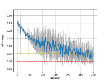
Figure 1. Advantage curve and margin histogram.

We select parameters for LazyBB and DP-LR entirely using grid-search and cross-validation (Table 1 for LazyBB) for each value of epsilon plotted i.e. $\epsilon\in(0.05,0.1,\cdots,0.5,1,3,5)$. Over the small datasets we use for experiments, the Weak Learner assumption does not hold for “long enough” to realize the training error guarantee of Theorem 5. For example, fixing $\kappa=1/2$ — seeking “good” margin on only half the training set — suppose we have a (1/20)-advantage Weak Learner. That is, at every round of boosting, each new hypothesis has accuracy at least 55% over the intermediate distribution. Under these conditions, Theorem 5 guarantees utility after approximately 4,000 rounds of boosting. Figure 1 plots advantage on the Adult dataset at each round of boosting with $\lambda=\gamma/4$ as required by Theorem 5, averaged over 10 runs of the boosting decision stumps with total privacy budget $\epsilon=1$. The weak learner assumption fails after only 250 rounds of boosting.

And yet, even when run with much faster learning rate $\lambda$, we see good accuracy from LazyBB — the assumption holds for small $\tau$, ensuring that DP-1R has advantage. So, Theorem 5 is much more pessimistic than is warranted. This is a know limitation of the analysis for any non-adaptive boosting algorithm Schapire and Freund (2012). In the non-private setting, we set $\lambda$ very slow and boost for “many” rounds, until decay in advantage triggers a stopping criterion. In the private setting (where non-adaptivity makes differential privacy easier to guarantee) running for “many” rounds is not feasible; noise added for privacy would saturate the model. These experiments motivate further theoretical investigation of boosting dynamics for non-adaptive algorithms, due to their utility in the privacy-preserving setting.

Low privacy regime
High privacy regime

Table 2. Learning Curves — Privacy vs. accuracy.

Results.

In Table 2 we plot the accuracy of each of the 5 methods above against privacy constraint $\epsilon$, along with two non-private baselines to both quantify the “cost of privacy” and ensure that the private learners are non-trivial. The strong non-private baseline is the implementation of Gradient Boosted Trees in sklearn, the weak non-private baseline is a single 1-Rule. It is important to note that for DP-Bag and DPBoost, we only compare our results for datasets and regimes that the corresponding hyperparameters are reported in the related works. Surprisingly, we found that LazyBB over 1-Rules and differentially private logistic regression were the best performing models — despite being the simplest algorithms to state, reason about, and run.

Sparsity, regularization, and interpretability.

Algorithms used for high-stakes decisions should be both well-audited and privacy-preserving. However, often there is a trade-off between privacy and interpretability Harder et al. (2020). Generally, noise injected to protect privacy harms interpretability. But our algorithms maintain accuracy under strong privacy constrains while admitting a high level of sparsity — which facilitates interpretability. Table 3 lists measurements across different levels of privacy. For an example of boosted one-rules at $\epsilon=0.4$ DP, see Table 4.

DP-LR — another simple algorithm with excellent performance — uses $L_{2}$ regularization to improve generalization. While $L_{2}$ regularization keeps total mass of weights relatively small, it generally assigns non-negligible weight to every feature. Hence, the resulting model becomes less interpretable as the dimension of data grows. On other hand, LazyBB with 1-Rules controls sparsity by the number of rounds of boosting. Just as with non-private non-adaptive boosting algorithms, we can see this as a greedy approximation to $L_{1}$ regularization of a linear model Rosset et al. (2004). Moreover, the final model can be interpreted as a simple integral weighted voting of features.

$\epsilon$	features count mean	features count std	% features
0.40	6.4	0.800	3.95%
0.50	12.8	0.400	7.90%
1.00	30.6	1.200	18.88%
3.00	72.8	2.481	44.93%
5.00	49.8	2.785	30.74%

Table 3. Statistics of number of features used by LazyBB with DP-1R across different levels of privacy on adult dataset. See the Appendix for the complete table.

votes	(feature, value)
3	marital-status : Married-civ-spouse
-2	capital-gain = 0
1	occupation : Exec-managerial
1	occupation : Prof-specialty
1	13 $\leq$ education-num $\leq$ 14.5
-1	age $\leq$ 17

Table 4. A $0.4$-DP model obtained by training LazyBB with DP-1R on adult dataset with $0.82$ accuracy.

Pessimistic Generalization Theory.

Empirically, LazyBB generalizes well. As with AdaBoost, we could try to explain this with large margins and Rademacher complexity, which applies to any voting classifier. So, we estimated the Rademacher complexity of 1-Rules over each dataset to predict test error. The bounds are far more pessimistic than the experiments; please see the Appendix for comparison tables. Intuitively, if LazyBB showed larger margins on the training data than on unseen data, this would constitute a membership inference attack — which is ruled out by differential privacy. This motivates theoretical investigation of new techniques to guarantee generalization of differentially private models trained on small samples.

6. Weighted Exponential Mechanism: Proof of Theorem 3

In this section we discuss the privacy guarantee of the Weighted Exponential Mechanism defined in Definition 2.4. Our proof follows the same steps as the standard Exponential Mechanism McSherry and Talwar (2007). Our goal is to prove, given two neighboring datasets and two similar distributions on them, the Weighted Exponential Mechanism outputs the same hypothesis with high probability.

In what follows let $M$ denote the Weighted Exponential Mechanism, and let $\mathcal{H}=\mathrm{Range}(M)$. Suppose $\mathcal{S},\mathcal{S}^{\prime}$ are two neighboring datasets of size $n$ and $\mu,\mu^{\prime}$ are distributions over $[n]$ such that $\mathtt{d}(\mu,\mu^{\prime})<\zeta$. Furthermore, let $q_{D,\mu}\colon\mathcal{H}\to\mathbb{R}$ be a quality score that has robust sensitivity $\Delta_{\zeta}$. That is, for every hypothesis $h\in\mathcal{H}$, we have

$$\max\limits_{\begin{subarray}{c}D\sim D^{\prime}\\ \mu,\mu^{\prime}:\mathtt{d}(\mu,\mu^{\prime})<\zeta\end{subarray}}|q_{D,\mu}(h)-q_{D^{\prime},\mu^{\prime}}(h)|\leq\Delta_{\zeta}.$$ (1)

We proceed to prove that for any $h\in\mathcal{H}$ the following holds

$$\Pr[M(S,\mu)=h]\leq\exp(2\eta\Delta_{\zeta})\Pr[M(S^{\prime},\mu^{\prime})=h].$$

Recall that $M$ outputs a hypothesis $h$ with probability proportional to $\exp(\eta\cdot q_{D,\mu})$ with $\eta=\frac{\epsilon}{2\Delta_{\zeta}}$. Let us expand the probabilities above,

$$\frac{\Pr[M(\mathcal{S},\mu)=h]}{\Pr[M(\mathcal{S}^{\prime},\mu^{\prime})=h]} =\frac{\exp{(\eta\cdot q_{\mathcal{S},\mu}(h))}}{\exp{(\eta\cdot q_{\mathcal{S}^{\prime},\mu^{\prime}}(h))}}$$

$$\times\frac{\sum\limits_{h\in\mathcal{H}}\exp{(\eta\cdot q_{\mathcal{S}^{\prime},\mu^{\prime}}(h))}}{\sum\limits_{h\in\mathcal{H}}\exp{(\eta\cdot q_{\mathcal{S},\mu}(h))}}.$$

Consider the first term, then

$$\frac{\exp{(\eta\cdot q_{\mathcal{S},\mu}(h))}}{\exp{(\eta\cdot q_{\mathcal{S}^{\prime},\mu^{\prime}}(h))}}=\exp{(\eta[q_{\mathcal{S},\mu}(h)-q_{\mathcal{S}^{\prime},\mu^{\prime}}(h)])}$$

$$\leq\exp{(\eta\cdot\Delta_{\zeta})}$$ (By (1))

Now consider the second term, then

$$\frac{\sum\limits_{h\in\mathcal{H}}\exp{(\eta\cdot q_{\mathcal{S}^{\prime},\mu^{\prime}}(h))}}{\sum\limits_{h\in\mathcal{H}}\exp{(\eta\cdot q_{\mathcal{S},\mu}(h))}}\leq\frac{\sum\limits_{h\in\mathcal{H}}\exp{(\eta\cdot[q_{\mathcal{S},\mu}(h)+\Delta_{\zeta}])}}{\sum\limits_{h\in\mathcal{H}}\exp{(\eta\cdot q_{\mathcal{S},\mu}(h))}}$$

$$=\frac{\exp{(\eta\Delta_{\zeta})}\sum\limits_{h\in\mathcal{H}}\exp{(\eta\cdot q_{\mathcal{S},\mu}(h))}}{\sum\limits_{h\in\mathcal{H}}\exp{(\eta\cdot q_{\mathcal{S},\mu}(h))}}$$

$$=\exp{(\eta\Delta_{\zeta})}$$

Hence, it follows that

$$\frac{\Pr[M(\mathcal{S},\mu)=h]}{\Pr[M(\mathcal{S}^{\prime},\mu^{\prime})=h]}\leq\exp{(\eta\Delta_{\zeta})}\cdot\exp{(\eta\Delta_{\zeta})}$$

$$=\exp{(2\eta\Delta_{\zeta})}$$

This implies that, for $\eta>0$, WEM is a $(2\eta\Delta_{\zeta},0,\zeta)$-differentially private weak learner. (Note that setting $\eta=\frac{2\epsilon}{2\Delta_{\zeta}}$ yields a $(\epsilon,0,\zeta)$-differentially private weak learner.)

We point out that the proof for the utility guarantee of Theorem 3 is identical to the proof of the utility guarantee in standard Exponential Mechanism McSherry and Talwar (2007).

7. Weighted Return Noisy Max: Proof of Theorem 4

In this section we discuss the privacy guarantee of the Weighted Return Noisy Max defined in Section 2.4. Our proof follows the same steps as the standard Return Noisy Max explained in Dwork and Roth (2014) with slight modification. Our goal is to prove, given two neighboring datasets and two similar distributions on them, the WRNM outputs the same hypothesis index.

Let $f_{1},\dots,f_{k}$ be $k$ quality functions where each $f_{i}:\mathcal{S}\times\mathcal{D}(S)\to\mathbb{R}$ maps datasets and distributions over them to real numbers. For a dataset $S$ and distribution $\mu$ over $S$, WRNM adds independently generated Laplace noise $Lap(1/\eta)$ to each $f_{i}$ and returns the index of the largest noisy function i.e. $i^{*}=\mathop{\mathrm{argmax}}\limits_{i}(f_{i}+Z_{i})$ where each $Z_{i}$ denotes a random variable drawn independently from the Laplace distribution with scale parameter $1/\eta$. In what follows let $M$ denote the WRNM.

Suppose $\mathcal{S},\mathcal{S}^{\prime}$ are two neighboring datasets of size $n$ and $\mu,\mu^{\prime}$ are distributions over $[n]$ such that $\mathtt{d}(\mu,\mu^{\prime})<\zeta$. Furthermore, suppose each $f_{i}$ has robust sensitivity at most $\Delta_{\zeta}$. That is, for every index $i\in\{1,\dots,k\}$, we have

$$\max\limits_{\begin{subarray}{c}D\sim D^{\prime}\\ \mu,\mu^{\prime}:\mathtt{d}(\mu,\mu^{\prime})<\zeta\end{subarray}}|f_{i}(\mathcal{S},\mu)-f_{i}(\mathcal{S}^{\prime},\mu^{\prime})|\leq\Delta_{\zeta}.$$ (2)

Fix any $i\in\{1,\dots,k\}$. We will bound the ratio of the probabilities that $i$ is selected by $M$ with inputs $\mathcal{S},\mathcal{S}^{\prime}$ and distributions $\mu,\mu^{\prime}$.

Fix $Z_{-i}=(Z_{1},\dots,Z_{i-1},Z_{i+1},\dots,Z_{k})$, where each $Z_{j}\in Z_{-i}$ is drawn from $Lap(1/\eta)$. We first argue that

$$\frac{\Pr[M(\mathcal{S},\mu)=i\mid Z_{-i}]}{\Pr[M(\mathcal{S}^{\prime},\mu^{\prime})=i\mid Z_{-i}]}\leq\mathrm{e}^{2\eta\cdot\Delta_{\zeta}}.$$

Define $Z^{*}$ to be the minimum $Z_{i}$ such that

$$f_{i}(\mathcal{S},\mu)+Z^{*}>f_{j}(\mathcal{S},\mu)+Z_{j}~{}~{}~{}\forall j\neq i$$

Note that, having fixed $Z_{-i}$, $M$ will output $i$ only if $Z_{i}\geq Z^{*}$. Recalling (2), for all $j\neq i$, we have the following,

$$f_{i}(\mathcal{S}^{\prime},\mu^{\prime})+Z^{*}+\Delta_{\zeta}\geq f_{i}(\mathcal{S},\mu)+Z^{*}>f_{j}(\mathcal{S},\mu)+Z_{j}$$

$$\geq f_{j}(\mathcal{S}^{\prime},\mu^{\prime})+Z_{j}-\Delta_{\zeta}$$

This implies that

$$f_{i}(\mathcal{S}^{\prime},\mu^{\prime})+Z^{*}+2\Delta_{\zeta}\geq f_{j}(\mathcal{S}^{\prime},\mu^{\prime})+Z_{j}$$

Now, for dataset $\mathcal{S}^{\prime}$, distribution $\mu^{\prime}$, and $Z_{-i}$, mechanism $M$ selects the $i$-th index if $Z_{i}$, drawn from $Lap(1/\eta)$, satisfies $Z_{i}\geq Z^{*}+2\Delta_{\zeta}$.

$$\Pr_{Z_{i}\sim Lap(1/\eta)}[M(\mathcal{S}^{\prime},\mu^{\prime})=i\mid Z_{-i}]$$

$$\geq\Pr_{Z_{i}\sim Lap(1/\eta)}[Z_{i}\geq Z^{*}+2\Delta_{\zeta}]$$

$$\geq\mathrm{e}^{-(2\eta\Delta_{\zeta})}\Pr_{Z_{i}\sim Lap(1/\eta)}[Z_{i}\geq Z^{*}]$$

$$=\mathrm{e}^{-(2\eta\Delta_{\zeta})}\Pr_{Z_{i}\sim Lap(1/\eta)}[M(\mathcal{S},\mu)=i\mid Z_{-i}]$$

Multiplying both sides by $\mathrm{e}^{(2\eta\Delta_{\zeta})}$ yields the desire bound.

$$\frac{\Pr_{Z_{i}\sim Lap(1/\eta)}[M(\mathcal{S},\mu)=i\mid Z_{-i}]}{\Pr_{Z_{i}\sim Lap(1/\eta)}[M(\mathcal{S}^{\prime},\mu^{\prime})=i\mid Z_{-i}]}\leq\mathrm{e}^{(2\eta\Delta_{\zeta})}$$

This implies that, for $\eta>0$, WRNM is a $(2\eta\Delta_{\zeta},0,\zeta)$-differentially private weak learner. (Note that setting $\eta=\frac{2\epsilon}{2\Delta_{\zeta}}$ yields a $(\epsilon,0,\zeta)$-differentially private weak learner.)

8. Weak Learner: DP 1-Rules

Throughout this section let $\mathcal{S}=\{(\mathbf{x}_{i},y_{i})\}^{n}$ where $\mathbf{x}_{i}=(x_{i1},\dots,x_{ir})$ denote a dataset, and let $\mu$ be a distribution over $[n]$. We will brute-force “1-Rules,” also known as Decision Stumps Iba and Langley (1992); Holte (1993). Here, these simply evaluate a single Boolean literal such as $\neg x_{17}$ — an input variable that may or may not be negated. We also admit the constants True and False as literals.

A brutally simple but surprisingly effective weak learner returns the literal with optimal weighted agreement to the labels. For any 1-Rule $h$ define $\mathrm{err}(\mathcal{S},\mu,h)$ to be:

$$\mathrm{err}(\mathcal{S},\mu,h)=\sum\limits_{(\mathbf{x}_{i},y_{i})\in\mathcal{S}}\mu(i)\chi\{h(\mathbf{x}_{i})\neq y\}.$$

For learning 1-Rules under DP constraints, the natural approach is to use the Exponential Mechanism to noisily select the best possible literal. There is a small type error: the standard Exponential Mechanism does not consider utility functions with an auxiliary weighting $\mu$. But for weak learning we only demand privacy (close output distributions) when both the dataset and measures are “close.” When both promises hold and $\mu$ is fixed, the Exponential Mechanism is indeed a differentially private 1-Rule learner. We show this formally below.

Let $\mathcal{S}\sim\mathcal{S}^{\prime}$ be any two neighboring datasets and set $I=\mathcal{S}\cap\mathcal{S}^{\prime}$. Then, for any two distributions $\mu,\mu^{\prime}$ over $[n]$, we have

$$\left|\mathrm{err}(\mathcal{S},\mu,T)-\mathrm{err}(\mathcal{S}^{\prime},\mu^{\prime},T)\right|$$

$$=\begin{multlined}\Bigg{|}\sum\limits_{(\mathbf{x}_{i},y_{i})\in\mathcal{S}}\mu(i)\chi\{T(\mathbf{x}_{i})\neq y\}\\ -\sum\limits_{(\mathbf{x}_{i},y_{i})\in\mathcal{S}^{\prime}}\mu^{\prime}(i)\chi\{T(\mathbf{x}_{i})\neq y\}\Bigg{|}\end{multlined}\Bigg{|}\sum\limits_{(\mathbf{x}_{i},y_{i})\in\mathcal{S}}\mu(i)\chi\{T(\mathbf{x}_{i})\neq y\}\\ -\sum\limits_{(\mathbf{x}_{i},y_{i})\in\mathcal{S}^{\prime}}\mu^{\prime}(i)\chi\{T(\mathbf{x}_{i})\neq y\}\Bigg{|}$$

$$=\begin{multlined}\Bigg{|}\sum\limits_{(\mathbf{x}_{i},y_{i})\in\mathcal{S}\cap\mathcal{S}^{\prime}}[\mu(i)-\mu^{\prime}(i)]\chi\{T(\mathbf{x}_{i})\neq y\}\\ +\sum\limits_{(\mathbf{x}_{i},y_{i})\in\mathcal{S}\triangle\mathcal{S}^{\prime}}[\mu(i)-\mu^{\prime}(i)]\chi\{T(\mathbf{x}_{i})\neq y\}\Bigg{|}\end{multlined}\Bigg{|}\sum\limits_{(\mathbf{x}_{i},y_{i})\in\mathcal{S}\cap\mathcal{S}^{\prime}}[\mu(i)-\mu^{\prime}(i)]\chi\{T(\mathbf{x}_{i})\neq y\}\\ +\sum\limits_{(\mathbf{x}_{i},y_{i})\in\mathcal{S}\triangle\mathcal{S}^{\prime}}[\mu(i)-\mu^{\prime}(i)]\chi\{T(\mathbf{x}_{i})\neq y\}\Bigg{|}$$

$$\leq\sum\limits_{(\mathbf{x}_{i},y_{i})\in\mathcal{S}\cap\mathcal{S}^{\prime}}|\mu(i)-\mu^{\prime}(i)|+\sum\limits_{(\mathbf{x}_{i},y_{i})\in\mathcal{S}\triangle\mathcal{S}^{\prime}}|\mu(i)-\mu^{\prime}(i)|$$

$$=\sum\limits_{i=1}^{n}|\mu(i)-\mu^{\prime}(i)|=2\mathtt{d}(\mu,\mu^{\prime}).$$

0:  Dataset $\mathcal{S}$, distribution $\mu$ over $[1,\dots,|\mathcal{S}|]$, and $\eta>0$.

1:  Let $\mathcal{H}$ be the set of all literals over $\mathcal{S}$ plus the constants True and False

2:  for $h\in\mathcal{H}$ do

3:     $q_{\mathcal{S},\mu}(h)\leftarrow-\mathrm{err}(\mathcal{S},\mu,h)$.

4:  end for

5:  $h_{out}\leftarrow$ select a hypothesis $h\in\mathcal{H}$ with probability proportional to $\exp{(\eta\cdot q_{\mathcal{S},\mu}(h))}$

6:  return $h_{out}$

Algorithm 3 Differentially Private 1-Rule Induction($\mathcal{S},\mu,\eta$)

Theorem 11.

Algorithm 3 is a $(4\eta\zeta,0,\zeta)$-differentially private weak learner.

Proof 8.1.

Suppose $\mathcal{S},\mathcal{S}^{\prime}$ are two neighboring datasets of size $n$ and $\mu,\mu^{\prime}$ are distributions over $[n]$ such that $\mathtt{d}(\mu,\mu^{\prime})<\zeta$. Observation 8 tells us that the quality score $q_{\mathcal{S},\mu}(h)=\mathrm{err}(\mathcal{S},\mu,h)$ has robust sensitivity $2\zeta$. Hence, by Theorem 3, we have that Algorithm 3 is a $(4\eta\zeta,0,\zeta)$-differentially private weak learner.

Theorem 12.

Let $h_{opt}$ denote the optimal hypothesis in $\mathcal{H}$. Then Algorithm 3, with probability at least $1-\beta$, returns $h_{out}\in\mathcal{H}$ such that

$$\mathrm{err}(h_{out})\leq\mathrm{err}(h_{opt})+\frac{1}{\eta}\ln{\frac{|\mathcal{H}|}{\beta}}.$$

Proof 8.2.

By Theorem 3, with probability at least $1-\beta$, we have

$$q_{\mathcal{S},\mu}(h_{out})\geq\max\limits_{h\in\mathcal{H}}q_{\mathcal{S},\mu}(h)-\frac{1}{\eta}\ln{\frac{|\mathcal{H}|}{\beta}}$$ (3)

Note that $q_{\mathcal{S},\mu}(h)=-\mathrm{err}(\mathcal{S},\mu,h)$ for all $h\in\mathcal{H}$ and $\max\limits_{h\in\mathcal{H}}q_{\mathcal{S},\mu}(h)=-\mathrm{err}(h_{opt})$. This gives us

$$-\mathrm{err}(h_{out})\geq-\mathrm{err}(h_{opt})-\frac{1}{\eta}\ln{\frac{|H|}{\beta}}\implies$$

$$\mathrm{err}(h_{out})\leq\mathrm{err}(h_{opt})+\frac{1}{\eta}\ln{\frac{|\mathcal{H}|}{\beta}}.$$

As we already discussed, in order to construct PAC learners by boosting weak learners we need weak learners that only beat random guessing on any distribution over the training set. Here, we wish to use Algorithm 3 as a weak learner. That is, we show that Algorithm 3 (with high probability) is better than random guessing. In what follows we have Theorem 8 and its proof.

Theorem 13.

Under a weak learner assumption with advantage $\gamma$, Algorithm 3, with probability at least $1-\beta$, is a weak learner with advantage at least $\gamma-\frac{1}{\eta}\ln{\frac{|\mathcal{H}|}{\beta}}$. That is, for any distribution $\mu$ over $\{1,\dots,|\mathcal{S}|\}$, we have

$$\sum\limits_{(\mathbf{x}_{i},y_{i})\in\mathcal{S}}\mu(i)\chi\{h_{out}(\mathbf{x}_{i})\neq y\}\leq 1/2-\left(\gamma-\frac{1}{\eta}\ln{\frac{|\mathcal{H}|}{\beta}}\right).$$

Proof 8.3.

By Theorem 12, Algorithm 3 with probability at least $1-\beta$ outputs a hypothesis $h_{out}$ such that

$$\mathrm{err}(h_{out})\leq\mathrm{err}(h_{opt})+\frac{1}{\eta}\ln{\frac{|\mathcal{H}|}{\beta}}.$$

Under a weak learner assumption, we assume that an optimal hypothesis $h_{opt}$ is at least as good as random guessing. That is $\mathrm{err}(h_{opt})<1/2-\gamma$. This yields the desired result.

9. Proof of Theorem 9

Here we consider splitting criterion to be the Gini criterion $G(q)=4q(1-q)$. Note that this function is symmetric about $1/2$ and $G(1/2)=1$. Throughout this section, $\mathcal{S}\sim\mathcal{S}^{\prime}$ are two neighboring datasets of size $n$ and $\mu,\mu^{\prime}$ are distributions over $[n]$ such that $\mathtt{d}(\mu,\mu^{\prime})<\zeta$. Observe that for a decision tree $T$ we have $|w(\ell,\mu)-w(\ell,\mu^{\prime})|\leq\zeta$ and $|q(\ell,\mu)-q(\ell,\mu^{\prime})|\leq\zeta$. Before proceeding to provide an upper bound on the sensitivity of $\mathrm{im}_{\ell,h,\mu}$, we prove some useful lemmas.

Lemma 14.

The following holds. 4—w(ℓ,μ)q(ℓ,μ)(1-q(ℓ,μ))- w(ℓ,μ’)q(ℓ,μ)(1-q(ℓ,μ’))— ≤54ζ

Proof 9.1.

As the Gini criterion $G(q)=4q(1-q)$ is symmetric about $1/2$, without loss of generality, we assume $q(\ell)\leq 1/2$. Furthermore, suppose $w(\ell,\mu)q(\ell,\mu)(1-q(\ell,\mu))$ is greater than $w(\ell,\mu^{\prime})q(\ell,\mu^{\prime})(1-q(\ell,\mu^{\prime}))$. The arguments for the other cases are analogous.

$$w(\ell,\mu)q(\ell,\mu)(1-q(\ell,\mu))-w(\ell,\mu^{\prime})q(\ell,\mu^{\prime})(1-q(\ell,\mu^{\prime}))$$

$$\leq w(\ell,\mu)q(\ell,\mu)(1-q(\ell,\mu))$$

$$\quad-w(\ell,\mu^{\prime})(q(\ell,\mu)-\zeta)(1-q(\ell,\mu)+\zeta)$$

$$=w(\ell,\mu)q(\ell,\mu)(1-q(\ell,\mu))$$

$$\quad-w(\ell,\mu^{\prime})q(\ell,\mu)(1-q(\ell,\mu)+\zeta)$$

$$\quad+w(\ell,\mu^{\prime})\zeta(1-q(\ell,\mu)+\zeta)$$

$$\leq w(\ell,\mu)q(\ell,\mu)(1-q(\ell,\mu))$$

$$\quad-w(\ell,\mu^{\prime})q(\ell,\mu)(1-q(\ell,\mu))+\zeta$$

$$\leq|w(\ell,\mu)-w(\ell,\mu^{\prime})|q(\ell,\mu)(1-q(\ell,\mu))+\zeta\leq\frac{5}{4}\zeta$$

Lemma 15.

For a decision tree $T$ and $(\ell,h)\in leaves(T)\times F$ we have

$$\Big{|}\mathrm{im}_{\ell,h,\mu}(\mathcal{S})-\mathrm{im}_{\ell,h,\mu^{\prime}}(\mathcal{S}^{\prime})\Big{|}\leq 4\zeta.$$

Proof 9.2.

For dataset $\mathcal{S}$ let $\mathcal{G}(T)=\sum\limits_{\ell\in leaves(T)}w(\ell)G(q(\ell))$. Recall the definition of $\mathrm{im_{\ell,h,\mu}}$,

$$\mathrm{im}_{\ell,h,\mu}(\mathcal{S}) =\mathcal{G}(T,\mu)-\mathcal{G}(T(\ell,h),\mu)$$

$$=w(\ell,\mu)G(q(\ell,\mu))-w(\ell_{0},\mu)G(q(\ell_{0},\mu))$$

$$-w(\ell_{1},\mu)G(q(\ell_{1},\mu))$$

Similarly, for dataset $\mathcal{S}^{\prime}$ let $\mathcal{G}(T,\mu^{\prime})=\sum\limits_{\ell\in leaves(T)}w(\ell,\mu^{\prime})G(q(\ell,\mu^{\prime}))$. Then we have

$$\mathrm{im}_{\ell,h,\mu^{\prime}}(\mathcal{S}^{\prime})=\mathcal{G}(T,\mu^{\prime})-\mathcal{G}(T(\ell,h),\mu^{\prime})$$

$$=w(\ell,\mu^{\prime})G(q(\ell,\mu^{\prime}))-w(\ell_{0},\mu^{\prime})G(q(\ell_{0},\mu^{\prime}))$$

$$\quad-w(\ell_{1},\mu^{\prime})G(q(\ell_{1},\mu^{\prime}))$$

Having these we can rewrite $\Big{|}\mathrm{im}_{\ell,h,\mu}(\mathcal{S})-\mathrm{im}_{\ell,h,\mu^{\prime}}(\mathcal{S}^{\prime})\Big{|}$ as follows,

$$\Big{|}\mathrm{im}_{\ell,h,\mu}(\mathcal{S})-\mathrm{im}_{\ell,h,\mu^{\prime}}(\mathcal{S}^{\prime})\Big{|}$$

$$=\Big{|}\mathcal{G}(T,\mu)-\mathcal{G}(T(\ell,h),\mu)-\mathcal{G}(T,\mu^{\prime})+\mathcal{G}(T(\ell,h),\mu^{\prime})\Big{|}$$

$$=\Bigg{|}w(\ell,\mu)G(q(\ell,\mu))-w(\ell_{0},\mu)G(q(\ell_{0},\mu))$$

$$\quad-w(\ell_{1},\mu)G(q(\ell_{1},\mu))-w(\ell,\mu^{\prime})G(q(\ell,\mu^{\prime}))$$

$$\quad+w(\ell_{0},\mu^{\prime})G(q(\ell_{0},\mu^{\prime}))+w(\ell_{1},\mu^{\prime})G(q(\ell_{1},\mu^{\prime}))\Bigg{|}$$

$$\leq\Big{|}w(\ell,\mu)G(q(\ell,\mu))-w(\ell,\mu^{\prime})G(q(\ell,\mu^{\prime}))\Big{|}$$

$$\quad+\Big{|}w(\ell_{0},\mu^{\prime})G(q(\ell_{0},\mu^{\prime}))-w(\ell_{0},\mu)G(q(\ell_{0},\mu))\Big{|}$$

$$\quad+\Big{|}w(\ell_{1},\mu^{\prime})G(q(\ell_{1},\mu^{\prime}))-w(\ell_{1},\mu)G(q(\ell_{1},\mu))\Big{|}$$

$$\leq 15/4\zeta\leq 4\zeta$$

where the last inequalities follow by Lemma 14.

Let us denote Algorithm 2 by $M$. Consider a fix decision tree $T$. We prove that, given $\mathcal{S}\sim\mathcal{S}^{\prime}$ and $\mu,\mu^{\prime}$, Algorithm 2 chooses the same leaf and split function with high probability.

Let $\mathcal{C}=leaves(T)\times F$ denote the set of possible split candidates. For each $(\ell,h)\in\mathcal{C}$, $\mathrm{im}_{\ell,h,\mu}(\mathcal{S})$ denotes the improvement gained in classification of dataset $\mathcal{S}$ by splitting $T$ at leaf $\ell$ according to split function $h$. Similarly, we have $\mathrm{im}_{\ell,h,\mu^{\prime}}(\mathcal{S}^{\prime})$. Provided that $\mathtt{d}(\mu,\mu^{\prime})\leq\zeta$, by Lemma 15, the robust sensitivity of quality score $\mathrm{im}_{\ell,h,\mu}$ is at most $4\zeta$. Similar to the proof of Theorem 3 it follows that

$$\frac{\Pr[M(\mathcal{S},\mu)=(\ell,h)]}{\Pr[M(\mathcal{S}^{\prime},\mu^{\prime})=(\ell,h)]}\leq\exp{(8\cdot\eta\cdot\zeta)}.$$

This means each selection procedure where DP-TopDown selects a leaf and a splitting function is $(8\cdot\eta\cdot\zeta,0,\zeta)$-differentially private. Using composition theorem for differentially private mechanisms, Theorem 1, yields privacy guarantee

$$\tilde{\epsilon}=8t\cdot\eta\cdot\zeta$$

for the construction of the internal nodes. We use $\tilde{\epsilon}$ for labeling the leaves using Laplace Mechanism. Since the leaves partition dataset, this preserves $\tilde{\epsilon}$-differential privacy by parallel composition of deferentially private mechanisms (Theorem 2). Overall, TopDown-DT is an $(16t\cdot\eta\cdot\zeta,0,\zeta)$-differentially private weak learner.

Remark 16.

Using advanced composition for differentially private mechanisms, Theorem 1, for every $\tilde{\delta}>0$ yields privacy guarantee

$$\tilde{\epsilon}_{\tilde{\delta}}=t(8\cdot\eta\cdot\zeta)^{2}+8\cdot\eta\cdot\zeta\sqrt{t\log(1/\tilde{\delta})}$$

for the construction of the internal nodes. We use $\tilde{\epsilon}_{\tilde{\delta}}$ for labeling the leaves using Laplace Mechanism. Since the leaves partition dataset, this preserves $\tilde{\epsilon}_{\tilde{\delta}}$-differential privacy by parallel composition of deferentially private mechanisms (Theorem 2). Overall, TopDown-DT is an $(2\tilde{\epsilon}_{\tilde{\delta}},\tilde{\delta},\zeta)$-differentially private weak learner.

10. Approximate Differential Privacy

Figures 2 and 3 compare the cross validation average accuracy on Adult dataset in the pure and approximate differential privacy regimes, for two different strategies of hyperparemeter selection: oblivious to $\epsilon$ (Figure 2), and $\epsilon$-dependent (Figure 3). This emphasizes the importance of tuning hyperparameters for each choice of $\epsilon$ separately. For approximate differential privacy, we consider the small constant value of $\delta=10^{-5}$, the same as that used by DP-Bag Jordon et al. (2019).

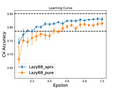
Figure 2. CV accuracy on Adult of $(\epsilon,\delta)$-DP LazyBB $(\kappa=1/4,~{}\lambda=1/4,~{}\tau=99)$ with DP-1R, $\delta\in\{0,10^{-5}\}$, varying $\epsilon$, vs. non-private baselines.

When we set hyperparameters identically for each $\epsilon$, using approximate differential privacy can allow significantly increased accuracy at each $\epsilon$. We found this to be the case especially for higher $\tau$; we select $\tau=99$ to illustrate. However, if we are allowed to separately optimize for each $\epsilon$, the significance of this advantage disappears. Though average accuracy clearly improves, it is not outside one standard deviation of average accuracy for pure differential privacy. It seems that boosted 1-Rules are too simple to distinguish between pure and approximate differential privacy constraints on this small dataset.

Figure 3. CV accuracy on Adult of $(\epsilon,\delta)$-DP LazyBB with DP-1R, $\delta\in\{0,10^{-5}\}$, varying $\epsilon$, vs. non-private baselines, with best model for each $\epsilon$ displayed.

Appendix A Sparsity statistics of the experiments

In Section 5, we discussed sparsity and interpretability of LazyBB with 1-Rules. Here we share the complete table of sparsity measurements for all the experiments. For each level of privacy, we use the hyper-parameter selected by cross-validation and repeated the experiment 5 times to obtain confidence bounds.

$\epsilon$	features count mean	features count std	% features
0.05	4.6	0.489	2.83%
0.10	4.8	0.400	2.96%
0.15	3.8	0.400	2.34%
0.20	3.6	1.019	2.22%
0.25	7.0	0.632	4.32%
0.30	13.8	1.166	8.51%
0.35	7.6	0.489	4.69%
0.40	6.4	0.800	3.95%
0.45	19.2	2.785	11.85%
0.50	12.8	0.400	7.90%
1.00	30.6	1.200	18.88%
3.00	72.8	2.481	44.93%
5.00	49.8	2.785	30.74%

Table 5. Sparsity measurements for Adult dataset.

$\epsilon$	features count mean	features count std	% features
0.05	6.0	0.632	7.50%
0.10	12.4	1.744	15.50%
0.15	19.6	1.625	24.50%
0.20	16.8	1.327	21.00%
0.25	11.2	0.748	14.00%
0.30	10.2	0.748	12.75%
0.35	26.4	1.356	33.00%
0.40	19.8	2.482	24.75%
0.45	34.4	1.497	43.00%
0.50	25.4	2.653	31.75%
1.00	54.2	3.187	67.75%
3.00	44.2	2.227	55.25%
5.00	32.0	2.098	40.00%

Table 6. Sparsity measurements for Cod-RNA dataset.

$\epsilon$	features count mean	features count std	% features
0.05	4.6	0.490	3.93%
0.10	7.2	1.166	6.15%
0.15	5.8	0.748	4.95%
0.20	8.6	1.497	7.35%
0.25	6.2	0.748	5.29%
0.30	5.6	0.490	4.78%
0.35	9.0	0.894	7.69%
0.40	9.8	1.166	8.37%
0.45	9.4	1.356	8.03%
0.50	11.8	1.720	10.08%
1.00	14.4	1.625	12.03%
3.00	28.8	2.926	24.61%
5.00	11.8	0.748	10.08%

Table 7. Sparsity measurements for Mushroom dataset.

Appendix B Hyperparameters

These are the hyperparemeters selected by cross-validation of boosted 1-Rules over each of our datasets. The privacy vs. accuracy curves use these settings for each value of $\epsilon$.

$\epsilon$	density	learning rate	no. estimators
0.05	0.50	0.50	5
0.10	0.45	0.50	5
0.15	0.50	0.40	5
0.20	0.50	0.30	5
0.25	0.35	0.50	9
0.30	0.40	0.40	19
0.35	0.30	0.45	9
0.40	0.35	0.50	9
0.45	0.40	0.45	25
0.50	0.35	0.50	15
1.00	0.35	0.45	39
3.00	0.35	0.45	99
5.00	0.35	0.45	75

Table 8. Hyperparameters selected by cross-validation for Adult dataset.

$\epsilon$	density	learning rate	no. estimators
0.05	0.50	0.50	9
0.10	0.50	0.35	19
0.15	0.50	0.50	29
0.20	0.40	0.50	25
0.25	0.50	0.45	25
0.30	0.50	0.45	25
0.35	0.45	0.35	49
0.40	0.45	0.45	39
0.45	0.50	0.40	65
0.50	0.45	0.50	49
1.00	0.40	0.50	99
3.00	0.30	0.40	99
5.00	0.35	0.40	99

Table 9. Hyperparameters selected by cross-validation for Cod-Rna dataset.

$\epsilon$	density	learning rate	no. estimators
0.05	0.45	0.50	5
0.10	0.50	0.40	9
0.15	0.50	0.45	9
0.20	0.50	0.40	15
0.25	0.30	0.40	9
0.30	0.35	0.50	9
0.35	0.40	0.35	15
0.40	0.45	0.40	19
0.45	0.35	0.20	19
0.50	0.45	0.25	25
1.00	0.25	0.30	29
3.00	0.20	0.20	75
5.00	0.20	0.50	29

Table 10. Hyperparameters selected by cross-validation for Mushroom dataset.

Appendix C Gap Between Theory and Experiments for Test Error

As discussed in section 5, there is a large gap between lower bounds predicted by large margin theory and Rademacher complexity, and the actual performance. The following table compares the best guaranteed lower bound derived by estimated Rademacher complexity and the test accuracy. The test accuracy of Adult dataset is obtained by evaluating the model on the test set, which was not touched during training. For Cod-RNA and Mushroom dataset there is no canonical test set available, so we report cross-validation accuracy.

Dataset	Rademacher Estimate of Test Accuracy	(CV) test accuracy
Adult	0.37	0.83
Cod-Rna	0.09	0.86
Mushroom	0.49	0.98

Table 11. Comparison between Rademacher estimates of generalization performance and experimental generalization performance for boosted 1-Rules, at $\epsilon=1$.

References

- Barak et al. (2009) B. Barak, M. Hardt, and S. Kale. The uniform hardcore lemma via approximate bregman projections. In C. Mathieu, editor, Proceedings of the Twentieth Annual ACM-SIAM Symposium on Discrete Algorithms, SODA 2009, New York, NY, USA, January 4-6, 2009, pages 1193–1200. SIAM, 2009. URL http://dl.acm.org/citation.cfm?id=1496770.1496899.
- Blum et al. (2005) A. Blum, C. Dwork, F. McSherry, and K. Nissim. Practical privacy: the sulq framework. In C. Li, editor, Proceedings of the Twenty-fourth ACM SIGACT-SIGMOD-SIGART Symposium on Principles of Database Systems, June 13-15, 2005, Baltimore, Maryland, USA, pages 128–138. ACM, 2005. 10.1145/1065167.1065184. URL https://doi.org/10.1145/1065167.1065184.
- Breiman et al. (1984) L. Breiman, J. H. Friedman, R. A. Olshen, and C. J. Stone. Classification and Regression Trees. Wadsworth, 1984. ISBN 0-534-98053-8.
- Bun and Steinke (2016) M. Bun and T. Steinke. Concentrated differential privacy: Simplifications, extensions, and lower bounds. In M. Hirt and A. D. Smith, editors, Theory of Cryptography - 14th International Conference, TCC 2016-B, Beijing, China, October 31 - November 3, 2016, Proceedings, Part I, volume 9985 of Lecture Notes in Computer Science, pages 635–658, 2016. 10.1007/978-3-662-53641-4_24. URL https://doi.org/10.1007/978-3-662-53641-4_24.
- Bun et al. (2020) M. Bun, M. L. Carmosino, and J. Sorrell. Efficient, noise-tolerant, and private learning via boosting. In J. D. Abernethy and S. Agarwal, editors, Conference on Learning Theory, COLT 2020, 9-12 July 2020, Virtual Event [Graz, Austria], volume 125 of Proceedings of Machine Learning Research, pages 1031–1077. PMLR, 2020. URL http://proceedings.mlr.press/v125/bun20a.html.
- Chaudhuri et al. (2011) K. Chaudhuri, C. Monteleoni, and A. D. Sarwate. Differentially private empirical risk minimization. J. Mach. Learn. Res., 12:1069–1109, 2011. URL http://dl.acm.org/citation.cfm?id=2021036.
- Dwork (2006) C. Dwork. Differential privacy. In M. Bugliesi, B. Preneel, V. Sassone, and I. Wegener, editors, Automata, Languages and Programming, 33rd International Colloquium, ICALP 2006, Venice, Italy, July 10-14, 2006, Proceedings, Part II, volume 4052 of Lecture Notes in Computer Science, pages 1–12. Springer, 2006. 10.1007/11787006_1. URL https://doi.org/10.1007/11787006_1.
- Dwork and Lei (2009) C. Dwork and J. Lei. Differential privacy and robust statistics. In M. Mitzenmacher, editor, Proceedings of the 41st Annual ACM Symposium on Theory of Computing, STOC 2009, Bethesda, MD, USA, May 31 - June 2, 2009, pages 371–380. ACM, 2009. 10.1145/1536414.1536466. URL https://doi.org/10.1145/1536414.1536466.
- Dwork and Roth (2014) C. Dwork and A. Roth. The algorithmic foundations of differential privacy. Foundations and Trends in Theoretical Computer Science, 9(3-4):211–407, 2014.
- Dwork et al. (2006) C. Dwork, K. Kenthapadi, F. McSherry, I. Mironov, and M. Naor. Our data, ourselves: Privacy via distributed noise generation. In S. Vaudenay, editor, Advances in Cryptology - EUROCRYPT 2006, 25th Annual International Conference on the Theory and Applications of Cryptographic Techniques, St. Petersburg, Russia, May 28 - June 1, 2006, Proceedings, volume 4004 of Lecture Notes in Computer Science, pages 486–503. Springer, 2006. 10.1007/11761679_29. URL https://doi.org/10.1007/11761679_29.
- Dwork et al. (2010) C. Dwork, G. N. Rothblum, and S. P. Vadhan. Boosting and differential privacy. In 51th Annual IEEE Symposium on Foundations of Computer Science, FOCS 2010, October 23-26, 2010, Las Vegas, Nevada, USA, pages 51–60. IEEE Computer Society, 2010. 10.1109/FOCS.2010.12. URL https://doi.org/10.1109/FOCS.2010.12.
- Friedman and Schuster (2010) A. Friedman and A. Schuster. Data mining with differential privacy. In B. Rao, B. Krishnapuram, A. Tomkins, and Q. Yang, editors, Proceedings of the 16th ACM SIGKDD International Conference on Knowledge Discovery and Data Mining, Washington, DC, USA, July 25-28, 2010, pages 493–502. ACM, 2010. 10.1145/1835804.1835868. URL https://doi.org/10.1145/1835804.1835868.
- Harder et al. (2020) F. Harder, M. Bauer, and M. Park. Interpretable and differentially private predictions. Proceedings of the AAAI Conference on Artificial Intelligence, 34:4083–4090, Apr. 2020. 10.1609/aaai.v34i04.5827. URL https://ojs.aaai.org/index.php/AAAI/article/view/5827.
- Holohan et al. (2019) N. Holohan, S. Braghin, P. M. Aonghusa, and K. Levacher. Diffprivlib: The IBM differential privacy library. CoRR, abs/1907.02444, 2019. URL http://arxiv.org/abs/1907.02444.
- Holte (1993) R. C. Holte. Very simple classification rules perform well on most commonly used datasets. Mach. Learn., 11:63–91, 1993. 10.1023/A:1022631118932. URL https://doi.org/10.1023/A:1022631118932.
- Hyafil and Rivest (1976) L. Hyafil and R. L. Rivest. Constructing optimal binary decision trees is np-complete. Inf. Process. Lett., 5(1):15–17, 1976. 10.1016/0020-0190(76)90095-8. URL https://doi.org/10.1016/0020-0190(76)90095-8.
- Iba and Langley (1992) W. Iba and P. Langley. Induction of one-level decision trees. In D. H. Sleeman and P. Edwards, editors, Proceedings of the Ninth International Workshop on Machine Learning (ML 1992), Aberdeen, Scotland, UK, July 1-3, 1992, pages 233–240. Morgan Kaufmann, 1992. 10.1016/b978-1-55860-247-2.50035-8. URL https://doi.org/10.1016/b978-1-55860-247-2.50035-8.
- Jordon et al. (2019) J. Jordon, J. Yoon, and M. van der Schaar. Differentially private bagging: Improved utility and cheaper privacy than subsample-and-aggregate. In Advances in Neural Information Processing Systems 32: Annual Conference on Neural Information Processing Systems 2019, NeurIPS 2019, December 8-14, 2019, Vancouver, BC, Canada, pages 4325–4334, 2019. URL https://proceedings.neurips.cc/paper/2019/hash/5dec707028b05bcbd3a1db5640f842c5-Abstract.html.
- Kasiviswanathan et al. (2011) S. P. Kasiviswanathan, H. K. Lee, K. Nissim, S. Raskhodnikova, and A. D. Smith. What can we learn privately? SIAM J. Comput., 40(3):793–826, 2011. 10.1137/090756090. URL https://doi.org/10.1137/090756090.
- Kearns and Mansour (1996) M. J. Kearns and Y. Mansour. On the boosting ability of top-down decision tree learning algorithms. In G. L. Miller, editor, Proceedings of the Twenty-Eighth Annual ACM Symposium on the Theory of Computing, Philadelphia, Pennsylvania, USA, May 22-24, 1996, pages 459–468. ACM, 1996. 10.1145/237814.237994. URL https://doi.org/10.1145/237814.237994.
- Levin and Peres (2017) D. A. Levin and Y. Peres. Markov chains and mixing times, volume 107. American Mathematical Soc., 2017.
- Li et al. (2020) Q. Li, Z. Wu, Z. Wen, and B. He. Privacy-preserving gradient boosting decision trees. In The Thirty-Fourth AAAI Conference on Artificial Intelligence, AAAI 2020, The Thirty-Second Innovative Applications of Artificial Intelligence Conference, IAAI 2020, The Tenth AAAI Symposium on Educational Advances in Artificial Intelligence, EAAI 2020, New York, NY, USA, February 7-12, 2020, pages 784–791. AAAI Press, 2020. URL https://aaai.org/ojs/index.php/AAAI/article/view/5422.
- McSherry (2010) F. McSherry. Privacy integrated queries: an extensible platform for privacy-preserving data analysis. Commun. ACM, 53(9):89–97, 2010. 10.1145/1810891.1810916. URL https://doi.org/10.1145/1810891.1810916.
- McSherry and Talwar (2007) F. McSherry and K. Talwar. Mechanism design via differential privacy. In 48th Annual IEEE Symposium on Foundations of Computer Science (FOCS 2007), October 20-23, 2007, Providence, RI, USA, Proceedings, pages 94–103. IEEE Computer Society, 2007. 10.1109/FOCS.2007.41. URL https://doi.org/10.1109/FOCS.2007.41.
- Pedregosa et al. (2011) F. Pedregosa, G. Varoquaux, A. Gramfort, V. Michel, B. Thirion, O. Grisel, M. Blondel, P. Prettenhofer, R. Weiss, V. Dubourg, J. Vanderplas, A. Passos, D. Cournapeau, M. Brucher, M. Perrot, and E. Duchesnay. Scikit-learn: Machine learning in Python. Journal of Machine Learning Research, 12:2825–2830, 2011.
- Quinlan (1986) J. R. Quinlan. Induction of decision trees. Mach. Learn., 1(1):81–106, 1986. 10.1023/A:1022643204877. URL https://doi.org/10.1023/A:1022643204877.
- Quinlan (1993) J. R. Quinlan. C4.5: Programs for Machine Learning. Morgan Kaufmann, 1993. ISBN 1-55860-238-0.
- Rokach and Maimon (2014) L. Rokach and O. Maimon. Data Mining with Decision Trees. WORLD SCIENTIFIC, 2nd edition, 2014. 10.1142/9097. URL https://www.worldscientific.com/doi/abs/10.1142/9097.
- Rosset et al. (2004) S. Rosset, J. Zhu, and T. Hastie. Boosting as a regularized path to a maximum margin classifier. J. Mach. Learn. Res., 5:941–973, 2004. URL http://jmlr.org/papers/volume5/rosset04a/rosset04a.pdf.
- Schapire and Freund (2012) R. E. Schapire and Y. Freund. Boosting: Foundations and Algorithms. The MIT Press, 2012. ISBN 0262017180.
- Wang et al. (2020) K. Wang, T. Dick, and M. Balcan. Scalable and provably accurate algorithms for differentially private distributed decision tree learning. CoRR, abs/2012.10602, 2020. URL https://arxiv.org/abs/2012.10602.
- Wood et al. (2018) A. Wood, M. Altman, A. Bembenek, M. Bun, M. Gaboardi, J. Honaker, K. Nissim, D. R. OBrien, T. Steinke, and S. Vadhan. Differential privacy: A primer for a non-technical audience. Vanderbilt Journal of Entertainment & Technology Law, 21(1):209–275, 2018.