Using Dynamic Binary Instrumentation to
Detect Failures in Robotics Software

Abstract

Autonomous and Robotics Systems are widespread, complex, and increasingly coming into contact with the public. Many of these systems are safety-critical, and it is vital to detect software errors to protect against harm.

We propose a family of novel techniques to detect unusual program executions and incorrect program behavior. We model execution behavior by collecting low-level signals at run time and using those signals to build machine learning models. These models can identify previously-unseen executions that are more likely to exhibit errors.

We describe a tractable approach for collecting dynamic binary runtime signals on ARSs, allowing the systems to absorb most of the overhead from dynamic instrumentation. The architecture of ARSs is particularly well-adapted to hiding the overhead from instrumentation.

We demonstrate the efficacy of these approaches on ArduPilot — a popular open-source autopilot software system — and Husky — an unmanned ground vehicle — in simulation. We instrument executions to gather data from which we build supervised machine learning models of executions and evaluate the accuracy of these models. We also analyze the amount of training data needed to develop models with various degrees of accuracy, measure the overhead added to executions that use the analysis tool, and analyze which runtime signals are most useful for detecting unusual behavior on the program under test. In addition, we analyze the effects of timing delays on the functional behavior of ARSs.

I Introduction

Autonomous and Robotics Systems (ARSs) are widespread, complex, and increasingly coming into contact with the public. Many of these systems are safety-critical, and it is vital to detect software errors to protect against harm [1, 2]. Significant challenges hamper efforts to ensure end-to-end safety in autonomous systems [3]. Such systems are often inaccessible and resource constrained (in terms of both power and computing resources), and typically make use of a mix of custom- and off-the-shelf components from a diversity of suppliers [4]. Use of proprietary components often means that source code is unavailable [5]. Similarly, it is typically difficult to adequately model certain system elements, especially continuous elements [6], for the purpose of formal verification. System correctness and safety thus requires a diverse array of assurance and analysis techniques, and those techniques typically cannot assume the availability of either source code or formal specifications for analysis.

However, robotics software also presents unique opportunities to leverage techniques that are not applicable or practical in standard software applications [5, 7]. In particular, we observe that, as parts of a real-time, distributed system, robotics system components often experience significant idle time waiting for events from other parts of the system or from the environment. This presents valuable unused capacity that can “hide” the overhead of tools that are impractical to use with CPU-, I/O-, or memory-bound software. We demonstrate some of this capacity experimentally.

With this opportunity in mind, our key insight is that Dynamic runtime characteristics can tell us about program behavior, from which we can build a machine-learning model of expected behavior. That is, by observing and measuring low-level execution signals such as number of machine instructions executed, we can effectively characterize program behavior over many executions. By combining these signals using machine learning, we can produce models that determine whether the current execution appears normal or anomalous, in terms of deviation from established patterns, [8]. These models can be used to predict whether new executions can be categorized as behaving as intended, or exhibiting errors. Our further insight is that the architecture of ARSs makes this approach tractable despite timing-sensitivity.

Marrying these two observations, in this paper, we present an approach we call for detecting errors in robotics systems. uses Dynamic Binary Instrumentation (DBI) to collect rich, low-level information about program behavior. We use machine learning to analyze and combine the signals into predictive models that identify whether an execution is nominal or anomalous.

At a high-level, DBI inserts code that analyzes a subject program while it executes. Although it is typically too heavy-weight an approach to be practical in many circumstances [5, 7], we find that robotics systems are well-suited to an approach that uses DBI appropriately, because they can absorb overhead in component idle time. We find this to be the case, even in cases when the timing of control loops has been tuned to avoid waste. Despite this opportunity, however, significant effort is required to still keep overhead tractable. Because they are real-time systems, robotics systems are sensitive to timing, sequencing, and deadline issues that can be affected by excessive instrumentation overhead.

We therefore develop a custom DBI tool we call SignalSeer using the Valgrind platform [9, 10] to efficiently collect selected runtime information that summarizes key characteristics of an execution’s behavior, such as the number of instructions executed or the maximum address of a memory load [11].

is applicable either at development- or run-time. At development time, in simulation or field testing, our techniques can detect unusual executions, providing the opportunity to repair any underlying faults in the software before deployment. Many errors in robotics software can be replicated in software simulation without full environmental replication [12, 13]. Discovering robotics faults early in simulation can reduce Quality Assurance (QA) costs as well as the cost of expensive field-test failures [14]. At run time, our techniques can detect unusual elements in executions before an error results in an outwardly-observable failure mode, providing the opportunity to stop the system or put it into a fail-safe mode. There are many use cases for alerts about unusual software behavior, intended or otherwise, including putting a critical system into a failsafe mode while a potential error is investigated [4], robustness testing [2, 15], and intrusion detection [16, 17, 18]. Additionally, is language-independent and operates at the binary execution level, without a need for source code, fitting the needs for analysis of many systems in the ARS domain.

Our work is complementary to previous work that has attempted to detect faulty program executions, some of which does so by establishing patterns of program behavior. Automated invariant detection techniques [8, 19, 20, 21, 22, 23] and statistical debugging techniques [24, 25, 26, 27] automatically identify properties that hold true over all correct executions of a program and identify bugs via violation of those invariants. However, such techniques typically require source code, can struggle to scale, or have other limitations which reduce their usefulness in complex autonomous systems. Formal verification of cyber-physical systems is powerful, but its practical application to entire real systems is limited. Models can include assumptions that do not necessarily hold true, have inadequate modeling of the physical world, and can require an extraordinary investment of time and human effort [6, 28, 29, 30, 31]. Related techniques are given a more complete treatment in Section VI.

We present as well-suited to robotics applications and test it on the ArduPilot software, which provides auto-pilot systems for various autonomous vehicles, as described in Section II-A. We evaluate it on indicative executions of ArduPilot, assessing the accuracy of the models’ output and evaluating training time and overhead. We show that is highly accurate at detecting executions that exhibit errors and detects those errors with minimal overhead. We further evaluate the extent to which overhead impacts observable robot execution.

The main contributions of this work are as follows:

• A tractable approach for using dynamic binary instrumentation as an analysis tool for robotics systems.

• An approach, , for using dynamic binary runtime signals as input to supervised machine learning techniques to detect unusual execution behavior.

• An evaluation of on simulations of the ArduPilot robotics software, to detect executions that exhibit unusual behavior.

• An evaluation of the amount of training data and overhead needed to use .

• An analysis of the dynamic binary runtime signals most useful for detecting unusual behavior in ArduPilot.

• An analysis of the effects of delays on the execution behavior of Husky, in support of the use of dynamic instrumentation as a tool for analyzing timing-critical systems.

II Background and Motivation

This section provides background for our work, including laying out details of the programs on which we evaluate our techniques: ArduPilot and Husky. It also walks through a motivating example, based on one of the experimental scenarios we evaluate for ArduPilot, and provides an introduction to Dynamic Binary Instrumentation (DBI).

II-A The Subject Systems

ArduPilot

We run the majority of our experiments on the ArduPilot system. This is an open-source project, written in C++, with autopilot systems that can be used with various types of autonomous vehicles. It runs a control loop architecture. ArduPilot is very popular with hobbyists, professionals, educators, and researchers and has approximately 678 thousand lines of code and over 50 thousand commits in its GitHub repository.

ArduPilot provides a rich ground on which to test robotics systems. It is sufficiently complex to be useful in the real-world. There is a wealth of information about bugs encountered in real world usage, both in the version-control history and in the academic literature [13]. We evaluate on ArduPilot in simulation, using the included software-in-the-loop simulator. We use a customized test harness that enables coordinated control over simulations.

For explanation and clarity, we present a simplified overview of relevant features of ArduPilot’s operation: ArduPilot executes startup commands to prepare the controller and start the autonomous vehicle. Then, if the system is in autopilot mode, the controller operates on a control loop. In practice, this means that the controller becomes ready to receive commands, one at a time, and executes them autonomously.

Husky

We evaluate the timing experiments on Husky.

The Husky unmanned ground vehicle by Clearpath Robotics is a real world robot with an extensive simulation infrastructure. It is rugged, designed to be deployed in uneven terrain, and it is capable of carrying and integrating with a variety of input sources (sensors) and actuators. Husky is popular among researchers for its straightforward design and real world usage history.

II-B Motivating Example

As a motivating example, we present a memory corruption bug in ArduPilot, specifically the ArduCopter software for autonomous control of airborne vehicles. The example we present here is based on a fault we seeded in early experiments with ArduCopter.

For each valid command received, the controller executes corresponding code, as defined in commands_logic.cpp. In this example, the code corresponding to a particular command — MAV_CMD_NAV_CONTINUE_AND_CHANGE_ALT — in commands_logic.cpp is seeded with a buffer overflow. This does not cause an externally-noticeable issue until the code corresponding to a different command — MAV_CMD_NAV_PAYLOAD_PLACE — attempts to read the data in the location that the overflow had written to.

At a low-level, looking at the pattern of memory writes can reveal the difference between the executions in which memory is corrupted and the executions in which it is not. For example, in the execution of the code corresponding to the command in which the memory is corrupted, there will be writes to memory addresses that are not usually written to in that part of the program. There may also be an unusually high number of memory writes. In addition, the difference may show up in other low-level indicators that we do not intuitively associate with buffer overflows.

uses machine learning techniques to look at all of the low level data collected by SignalSeer together. This gives us the benefit of not needing to know in advance which of the indicators may be relevant to any given bug.

In addition, monitoring low-level signals has the potential to detect this issue before there is an externally-visible problem by analyzing data collected after the buffer overflow is written but before the program gets to the code in which the corrupted memory is accessed. If we collect signals through the execution of the command MAV_CMD_NAV_CONTINUE_AND_CHANGE_ALT but analyze them before the execution of MAV_CMD_NAV_PAYLOAD_PLACE, the approach has the potential to detect the problem that has already been set up but has not yet caused any externally-observable effects. This flexibility can allow to detect errors before they manifest as user-observable crashes.

II-C Dynamic Binary Instrumentation

Dynamic Binary Instrumentation (DBI) works by analyzing a System Under Test (SUT) at execution time. The DBI analysis tool inserts code — instrumentation — that analyzes the SUT, to be run while the SUT runs. Because DBI works at runtime, it can encompass any code called by the subject program, whether it be within the original program, in a library, or elsewhere [10, 9, 32].

As a dynamic binary instrumentation framework, Valgrind allows tools based on the platform to record data about low-level events that take place during a program’s execution. Tools based on Valgrind can have significant overhead, although optimizations can reduce that overhead. For example, running the example tool, Lackey, and memory checking tool, Memcheck, that are distributed with Valgrind on a simple command in a basic Linux utility results in a 404x and 383x overhead, respectively, as measured by execution time. Our custom tool based on Valgrind incurs 186x overhead on this same command. The overhead for these tools on ArduPilot is significantly smaller, as discussed in Sections IV-D and IV-E, inspiring the use of DBI for robotics systems. We describe engineering considerations that make it possible to use a Valgrind tool on a robotics system in Section III-B.

III Approach

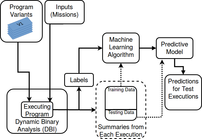
Figure 1: General Overview of the Supervised Learning Approach

In this section, we describe our approach for identifying software errors using supervised learning models built over low-level dynamic signals. We envision this technique — — to be used either at development time or during field testing. At development time, can be used on robot executions in simulation, to detect potential errors before deployment on real hardware. In deployed hardware during field testing, can be used to issue alerts regarding probable software errors, which can be addressed by putting the software or system into a fail safe mode while the problem is addressed.

We explain with reference to Figure 1, which lays out the architecture of the approach. We begin by generating a corpus of data that includes software executions that exhibit an error and executions that do not. Details about options for generating this corpus are in Section III-C. For the purpose of the experiments in this paper, we begin generating the corpus with with a base version of the SUT. From the base version, we generate mutant program variants using a systematic mutation approach. We also have a set of program inputs, which we can think of as defect-revealing inputs and non-defect-revealing inputs. As illustrated in Figure 1, each program variant is executed with each input.

We monitor these executions with a custom dynamic binary analysis (DBI) tool — SignalSeer— as described in Section III-A. The tool produces a summary of each execution, which consists of a set of counts and extremes of various events that occur at runtime. We call these pieces of data signals.

When each execution runs with a given input, we assign it a label of pass or fail, corresponding to whether the execution exhibited expected behavior. These labels are necessary as input to the supervised learning algorithms we use. We also use the labels to evaluate the success of our techniques. Using labeled data as input is a common technique, and labels for training data can be obtained in many ways.

We use the sets of signals as input to a supervised machine learning algorithm. This algorithm generates a predictive model. The predictive model takes, as input, test data — signals from executions that were not included in the data used to build the model. The model outputs a boolean prediction in the form of a 1 or 0 as to whether each of those sets of signals corresponds to an execution that exhibits an error.

III-A Collecting Signals with Dynamic Binary Instrumentation

To record low-level information about program executions, we developed a custom tool — SignalSeer— based on the Valgrind framework, version 3.14. As a DBI framework, Valgrind allows tools based on the platform to record data about low-level events that take place during a program’s execution. Examples of such low-level events are the execution of a single instruction or a single load from memory into a register.

We use DBI to collect signals that summarize the behavior of the execution monitored. The signals are chosen to be potentially informative while being easy to collect within the Valgrind framework and incurring very little calculation or data storage overhead at runtime. We discuss these choices in Section III-B. These counts result in a summary of each execution, consisting of a list of numbers, corresponding in order to the set of properties measured.

Our DBI tool outputs these summaries at intervals throughout the execution. Each signal is measured cumulatively from the beginning of the execution. By analyzing the summaries of signals at each interval, our technique can detect executions that exhibit defects that occur in the execution time covered by each interval. As discussed in Section II-B, unusual low-level behavior can occur well before an error is outwardly-visible.

We collect the same measurements for each summary, so the summary can be treated as a feature vector, suitable for input into machine learning algorithms. We aggregate the feature vectors over many executions into two-dimensional matrices, representing the overall data set.

In all, this customized tool outputs 26 signals. These signals include: counts of machine instructions executed, basic blocks entered and exited, load and store instructions executed, and events tracked internally by Valgrind; and minima, maxima, and ranges of addresses of machine instructions executed and data loaded and stored. It is possible to obtain accurate results with a subset of these signals, as discussed in Section IV-F. Our experiments use all 26 of these signals unless otherwise specifically mentioned.

III-B Minimizing Overhead in Dynamic Binary Instrumentation

One key difficulty in using a dynamic binary instrumentation approach with a timing-sensitive system is that the overhead of collecting the information changes the timing in the program execution. For example, ArduPilot has several timeout windows during which it expects certain events to happen; if they do not, the system aborts. We used several approaches in tool design to tractably reduce overhead:

Optimize to the basic block level whenever possible. Minimizing runtime interruptions is key to reducing instrumentation overhead. One established approach is to restrict interruptions to once per basic block, rather than every instruction. At the basic block level, it is possible to collect a summary of the events that occur within that block. However, not all information we wish to collect is available at the basic block level. For example, addresses that are computed at runtime may not be available. We, therefore, optimize instrumentation to the basic block level when all of the information we want is available at that level, such as when the block does not rely on any addresses computed at runtime. Otherwise, we instrument instructions within the block individually.

Eliminate excess data storage at instrumentation site. The amount of data associated with instrumentation (stored and retrieved at runtime) can drastically influence the overhead. We experimented with an approach that collected richer data by storing histograms of many data points. These included instruction addresses, memory addresses, and data values, along with more esoteric data; we used the histograms to calculate summary signals, such as the most frequent value. However, the memory usage and library calls involved in storage and updating the histograms slowed the instrumentation dramatically. Ultimately, simple tallies that involved a minimum of data storage and operations at runtime proved more tractable.

Avoid high-overhead Application Programming Interface (API) calls and computation at instrumentation sites. Because we must add many instrumentation sites, the overhead at each site must be minimal. Fortunately, not all low-level events are equally expensive (in time and data) for Valgrind to measure. For example, counts of information that require additional calls into the Valgrind API, such as some branch prediction information, are more expensive to collect than counts of information already available to the tool at an instrumentation site, such as the address of the current instruction. We restrict the events we measure to those that can be measured with a minimum of added overhead. For example, we do collect the address and type of each instruction. We do not collect data related to the order of memory events that would be useful if we were explicitly tracking memory exceptions.

Overall, instead of tracking high-overhead information, we take best advantage of each instrumentation site by collecting as much information as possible that is available with minimal calculation. To do this, we build SignalSeer on top of Valgrind’s Nullgrind tool, a tool designed to do nothing. We collect data on events tracked by Valgrind internally because those data are readily available. We keep a count of various types of instructions instrumented, even when those types of instructions are internal Valgrind bookkeeping instructions that do not correspond to machine instructions. We track these because it does not cost any additional overhead, and they may correspond to useful information.

III-C Corpus Generation

Using requires a corpus of labeled data for supervised learning, which we discuss in Section III-D. Generating this corpus of data requires a SUT that can be executed under DBI and a way of labeling each execution as exhibiting intended or unintended behavior. The corpus must contain at least some data corresponding to executions with intended behavior and some data corresponding to executions with unintended behavior. Examples from both classes are needed for the two-class supervised learning algorithms used as a part of .

There are many possible ways to generate a set of executions of the SUT that includes both well-behaved and misbehaving executions. Some SUT contain faults in their code as written and, when executed with an appropriate input, will exhibit errors. Another way to obtain executions that exhibit errors is to seed faults into the underlying program code. Again, with an appropriate input, the execution will exhibit an error. Ways to seed faults include mutating the programs using techniques common in mutation testing or seeding a known error into the code. One way to seed a realistic error is to use the edit history of a program’s source code to find a change that repaired a bug, then re-introduce the corresponding ‘buggy’ code into the SUT [33]. Note that obtaining faulty executions by seeding faults does not limit to only programs for which source code exists because faults can be seeded at any level, including in machine code. An additional way to obtain executions that exhibit errors is to include several versions from the version history of the same program, as long as those versions are sufficiently similar to one another to compare executions.

For our experiments, we generate the corpus by taking the base program as ArduPilot 3.6.7. We generate mutants using established techniques in mutation testing, with a primitive set of source code mutation operators used in prior studies [34]. We construct each mutant by applying a single mutation operator to a location in a core source file. We construct one such mutant for every combination of applicable location and mutation operator in several core source files. We use BugZoo [35] to create an ephemeral Docker container for each mutant under test. We execute each mutant with a suite of three inputs, which in the case of ArduPilot are known as missions, and discard data for any mutants that fail to compile and for any executions that crash immediately when executed. This results in 1778 execution traces. We then use a simple oracle to classify the traces as correct (pass) or erroneous (fail) based on the simulated physical location of the robot during the mission. Following this classification, we are left with 1658 correct and 120 erroneous traces. To avoid issues of class balance which can bias machine learning training, we balance all data by duplication of pseudo-randomly chosen data points in the minority class. We choose to balance by duplication because it does not reduce the size of the data set; our preliminary experiments show comparable results with balancing by deletion, when the data set is large enough. We balance the data separately for each model we build, and balance each fold separately for K-fold cross validation, to avoid the possibility of duplication resulting in the same summary appearing in the training corpus and test inputs.

III-D Supervised Learning

Supervised learning is a technique for developing machine learning models to classify data. We use two-class supervised learning, which means that the data falls into two categories. In this case, the categories are pass (0), which corresponds to executions that exhibit intended behavior, and fail (1), which corresponds to executions that exhibit unintended behavior. A supervised learning algorithm takes, as input, labeled data in the form of feature vectors — which in this case are the summaries output by our custom DBI tool SignalSeer— each of which has a corresponding 0 or 1, indicating the category to which the corresponding data belongs. That is, data that came from executions that were known to exhibit an error have the label 1, while the rest of the data came from executions that were not known to exhibit an error. We used a simple oracle of our own design to generate the labels, otherwise known as ground truth. This input data is known as training data. The labels for training data could come from the use of test cases, human observation of execution behavior, or other sources of knowledge of whether an execution is correct.

The supervised learning algorithm outputs a classifier. The classifier takes, as input, test data which consists of feature vectors – summaries – in the same form as those used to train the classifier but that were not used to train the classifier. The test data does not include labels. The classifier outputs predictions – determinations as to which class each data point belongs to. The term predictions is a term of art in machine learning that refers to the output of a classifier; it does not necessarily refer to future events. We assess the accuracy of the classifier by comparing the predictions to the known ground truth, which we obtain from our simple oracle. We discuss accuracy metrics in Section IV.

For supervised learning, we use use out-of-the box algorithms from Scikit Learn, version 0.15.2. Specifically, we use the Decision Tree classifier available from Scikit Learn. Based on an informal survey of the options available from Scikit Learn, we found that the Decision Tree classifier performs similarly to or better than other algorithms when used as a part of this technique, across a wide range of programs and data. We use the default parameters of the algorithm.

III-E Approach and Methodology for Timing Experiments

To evaluate the extent to which timing delays deform the observable execution of an ARS, we use a different set of experiments, in which we insert artificial timing delays in a controlled manner.

For a given robot, we establish a set of commands, called a mission. For the purposes of these experiments, each mission is represented as a series of destinations in three dimensional space (two dimensional space for robots that move in only two dimensions), with the final destination being a return to the first destination. We create a series of missions within a simulation environment for each robot.

The experiments consist of running two types of executions: nominal baseline executions in which the system is run without modifications and experimental executions in which the system is run with artificially-inserted timing delays.

Nominal Baseline Executions

To establish a nominal baseline — a baseline for how a robot behaves under normal conditions, without any artificially-inserted delays — we run each unmodified ARS repeatedly on each of its missions.

The executions to establish a nominal baseline serve several purposes in these experiments. First, the nominal executions establish a baseline for how often the unmodified ARS fails. ARSs often behave in a nondeterministic manner, even in simulation. There can be nominal (unmodified) executions that fail in significant ways, such as failing to reach one or more waypoints; getting “stuck” and discontinuing attempts to follow the mission (e.g., when the perception system cannot determine the robot’s location); software crashes; or liveness failures (e.g., hitting a timeout). The number of failures in the nominal, unmodified system establishes a point of comparison by which to measure the failure rate of the artificially-modified system. As a generalized approximate metric of these failures, we use the percent of executions in which the robot never reaches the final waypoint. This metric allows comparison between the failure rate in nominal executions and the failure rate in the modified system.

Second, the nominal executions establish a representative trajectory and other execution characteristics against which the characteristics of modified executions can be compared. Other potential characteristics of interest include the time taken for completion of the mission and the rate at which messages are sent on various topics.

Third, the nominal executions establish the range of variation in nominal trajectories and other execution characteristics. As mentioned above, there is significant nondeterminism in the observed behavior of simulated robots, even when unmodified. Establishing the range in the nominal executions provides a basis to tell when the modified, experimental executions are within the range of nominal behavior or outside of it.

Experimental Executions

For the experimental executions, we add controlled artificial delays to the execution of the ARS code. The experimental parameters include: the points within the program at which these delays are inserted, the number of insertion points, and the length of delays. The method of inserting delays is set out below.

Experimental executions are evaluated against the nominal baseline and against the set of waypoints that the simulated robot is directed to reach.

III-E1 Subject Systems

In addition to the ArduCopter ArduPilot system, which features heavily in the other experiments in this paper, we also evaluate on a Robot Operating System (ROS)-based system: Husky, to demonstrate the generalization of the timing absorption to other ARS.

III-E2 Method of Inserting Delays

This subsection explains how artificial delays are inserted for the experimental executions.

ArduCopter

For the ArduCopter experiments, the artificial delays are introduced by modifying source code in C++ and inserting sleep statements. We identify the program point before each return statement in all .cpp files in the ArduPilot/ArduCopter source code directory. Each of these program points was a possible location to insert a delay. The choice of whether to insert a delay at each point was determined probabilistically, with a weighted coin flip. Different modified versions of the code were created,  each of which had (a) a fixed coin flip weight and (b) fixed delay amount added at each delay location. The weights for the weighted coin flip ranged from 0.1 to 1.0, with 1.0 meaning a delay was inserted before every return statement, and the length of each delay ranged from 0.001953125 seconds to 8 seconds, with delay lengths chosen as powers of 2.

Husky

We conducted similar experiments on Husky, which is a system based in ROS. For the ROS experiments, the artificial delays are introduced at communications barriers on ROS topics, taking advantage of the architecture of ROS-based systems.

To give a simplified overview of the architecture of ROS-based systems as they relate to these inserted delays, these systems consist of various nodes that communicate with each other by sending messages over a bus, as shown in Figure 2.

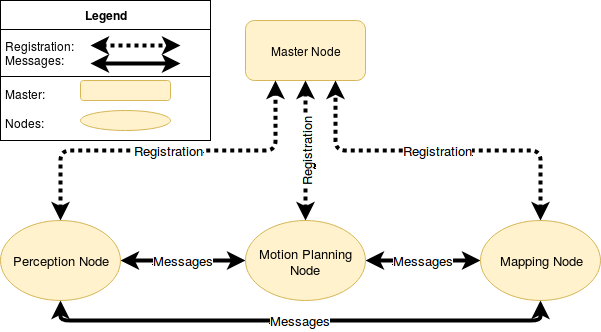
Figure 2: Simplified ROS Architecture

A publish-subscribe system determines which nodes receive which messages. A node can publish messages to a topic. To receive those messages, another node subscribes to the same topic. Generally, each topic only accepts messages of one type. ROS makes it easy to query a running system to find out configuration information such as (a) the topics in that system; (b) the type of messages published to each topic; (c) the node or nodes that publish to a given topic; and (d) the node or nodes that subscribe to the given topic. This information makes it easy to infer certain properties about the relationships among nodes and the purposes of particular messages. We use this information to choose the topics to which we add artificial delays. For example, in Husky, we run a set of experiments that delay each topic published by or subscribed to by the /move_base/ navigation node. We make this choice because navigation is a vital function, and we expect disruptions in navigation to have an effect on robot behavior. By contrast, we do not conduct experiments in which we delay the topics related to displaying logging messages, as we do not expect these delays to affect the robot’s functional behavior.

Having chosen a topic or topics to delay on a particular ROS system for a particular set of experiments, we insert delays on these topics by intercepting messages using topic renaming. ROS allows configuration of nodes such that topics can be renamed. For example, if Node A is originally designed to publish a topic named /a_very_good_topic, we can change the system’s configuration so that when published, the topic is known in the namespace as something else, such as /a_very_good_topic_intercepted. Because the topic now has a different name than other components in the system expect, the node or nodes that would have originally subscribed to the topic will not receive the messages published on the new topic. However, the delay infrastructure includes an additional node to be included with the ROS system. This node reads each message on a given topic, in this case /a_very_good_topic_intercepted. It then waits for the designated amount of time and then republishes the same message on the topic that was originally expected: /a_very_good_topic. The nodes that originally expected the messages on this topic from Node A now receive the same messages from the delay node.

Delays range in length from 0.00390625 seconds to 1 second, chosen as powers of two, and were inserted for every message in a topic. This range was chosen after a parameter sweep revealed that they result in a representative range of behaviors.

IV Evaluation

Using ArduPilot 3.6.7 as a case study system, we evaluate claims in two major areas: (A) Performance and accuracy, and (A) Effects of overhead. we ask the following research questions.

Performance and Accuracy

• RQ1: To what extent can accurately detect executions that exhibit errors?

• RQ2: How does the volume of training data used to build the model affect the accuracy of the model in detecting executions that exhibit errors?

• RQ3: To what extent can accurately detect executions that exhibit errors before reaching the end of the execution?

Effects of Overhead

• RQ4: How much overhead is introduced by DBI?

• RQ5: What effects do delays have on observable robot performance?

• RQ6: To what extent does feature reduction affect overhead and accuracy?

We run all experiments on an Ubuntu 16.04 virtual machine with 4 virtual cores and and 11GB RAM, running on a physical machine with an Intel(R) Xeon(R) E5620 CPU (2.40GHz).

We assess the performance of the models produced by with respect to their ability to correctly and generally label a set of traces. Given a set of test data, known labels, and the classifier’s predictions on the test data, the predictions can be evaluated into true and false positives and negatives (TP, FP, TN, and FN). Subsequent metrics include:

• Accuracy (Acc) The portion of samples whose predicted labels match the ground-truth labels: $(TP+TN)/(TP+FP+TN+FN)$.

• Precision (Prec) The ratio of returned labels that are correct: $TP/(TP+FP)$.

• Recall (Rec) The ratio of true labels that are returned: $TP/(TP+FN)$.

• F-Score (F) The harmonic mean of precision and recall, which guards against trivially maximizing precision or recall by predicting the labels to be all negative or all positive. Calculated as: $2*((Prec*Rec)/(Prec+Rec))$.

Unless otherwise stated, we use K-fold cross-validation, with K=10 for all sample sizes greater than or equal to 100. For smaller sample sizes, we use the largest K that ensures each fold has at least 10 points. We report the arithmetic mean across all folds.

IV-A RQ1: Error Detection

We answer RQ1: To what extent can accurately detect executions that exhibit errors?

Recall that our overall goal is to determine whether — an approach that combines dynamic-binary-instrumentation with machine-learning analysis — is useful in detecting behavior that exhibits defects in software. This question evaluates the overall suitability of this approach to detect errors in completed program executions. To answer this question, we take the approach described in Section III and evaluate it on the data for all executions in our corpus, as described in Section III-C. For this question, we use the cumulative signals recorded at the end of each execution.

We measure Accuracy, Precision, Recall, and F-Score, as described in Section III-D. We report the means across 10-fold cross-validation. For each metric, higher is better and means that the technique’s determinations are more accurate.

Table I shows results. We find that we can build a strong classifier that detects errors in complete ArduPilot executions. The precision is nearly perfect, which means that there are very few false positives. This classifier works across different defects and missions, supporting its generality.

TABLE I: Accuracy Metrics for Supervised Learning using Data at the End of Execution

Mean	Mean	Mean	Mean	Num.
Acc.	Prec.	Rec.	F-Score	Samples
0.95	0.99	0.90	0.94	1778

IV-A1 Using a Prior Release to Detect Errors on a Subsequent Release

We ask a related question: Can a model trained on executions of a prior release of the software under test identify errors in a subsequent release of the software?

We answer this question by training a model on a set of executions on ArduPilot version 3.6.6 and testing it on executions from version 3.6.7. The model trained on ArduPilot 3.6.6 uses 280 data points drawn from sampling 185 mutations across three missions. We do not use K-fold cross validation to assess the accuracy of these models because the training and test data are drawn from different data sets. We test on 1778 data points from the data set drawn from executions of ArduPilot 3.6.7. Results are in Table II.

TABLE II: Accuracy Metrics for Supervised Learning Trained on a Prior Version (ArduPilot 3.6.6) and Tested on a Subsequent Version (ArduPilot 3.6.7).

Mean	Mean	Mean	Mean	Num.	Num.
Acc.	Prec.	Rec.	F-Score	3.6.6	3.6.7
0.90	0.99	0.82	0.90	280	1778

By comparing the results for this experiment (Table II) with the the accuracy for the model trained and tested from the data drawn from the same set (Table I), we find that the accuracy metrics show that this model is highly accurate, and only slightly less accurate than a model trained and tested on data drawn from only one version of the software. Part of the decrease in accuracy may be attributable to the smaller number of data points used to train this model, rather than to the different version.

This results illustrates a promising use case for in the software development pipeline. While developing software, a model can be trained on executions from a prior release of the software. While developing subsequent versions, the model can be used to assess executions from the changed software for errors such as regressions. This approach should apply to many situations in which the software under development is similar to its prior release.

IV-B RQ2: Amount of Training Data and Accuracy

We answer RQ2: How does the volume of training data used to build the model affect the accuracy of the model in detecting executions that exhibit errors? Recall that our overall goal is to determine whether is useful in detecting software executions that exhibit errors. This question evaluates the subgoal of determining how much data is necessary to make useful predictions. To answer this question, we compute the analyses used to evaluate RQ1 in Section IV-A with varying amounts of data.

We show results for all accuracy metrics in Table III and graph results for the F-Score metric in Figure 3. Higher is better. The X-axis represents the total number of samples included for supervised learning. (The samples are split between training and testing samples for K-fold cross-validation.) While results for 200 and 300 are middling, F-Score quickly rises to 0.90 at 400 samples and stays above 0.80 at all sample sizes above 400. These results show that can obtain reasonable accuracy with comparatively few data points. Computing 400 data points would take approximately 1274.55 minutes or less than a day. The F-Score does not fall below 0.90 after 1500 data points. Computing 1500 data points would take approximately 4779.55 minutes or a little more than three days. Such training time could become part of the workflow for a development or testing procedure. This is especially the case because, as demonstrated in Section IV-A1, such a model does not need to be trained on an identical version of the software to be effective, so a model built on an earlier version of software can continue to be used for subsequent development.

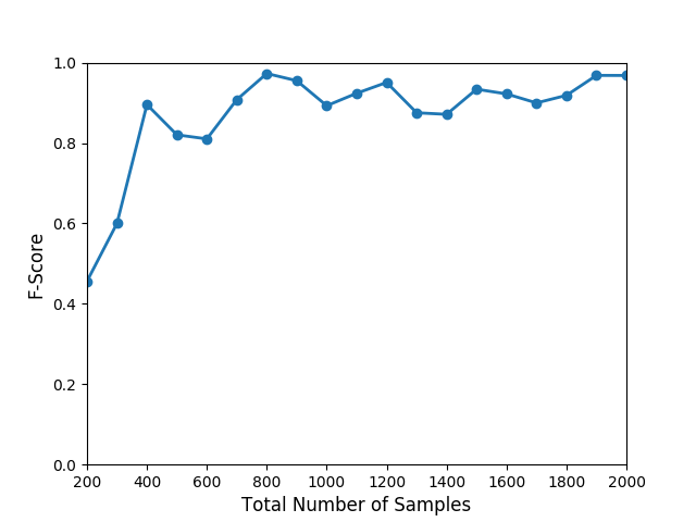
Figure 3: Supervised Learning with Varied Amounts of Data

TABLE III: Accuracy Metrics and Approximate Training Time for Varying Numbers of Data Points.

Num.	Mean	Mean	Mean	Mean	Data Gen.
Samples	Acc.	Prec.	Rec.	F-Score	Time (mins)
200	0.90	0.50	0.43	0.46	637.27
300	0.89	0.65	0.59	0.60	955.91
400	1.00	0.90	0.89	0.90	1274.55
500	0.94	0.89	0.78	0.82	1593.18
600	0.93	0.89	0.76	0.81	1911.82
700	0.92	0.98	0.86	0.91	2230.45
800	0.98	0.99	0.96	0.97	2549.09
900	0.96	0.99	0.93	0.96	2867.73
1000	0.91	0.99	0.84	0.89	3186.36
1100	0.94	0.99	0.89	0.92	3505.00
1200	0.96	0.99	0.92	0.95	3823.64
1300	0.89	0.98	0.80	0.88	4142.27
1400	0.90	0.99	0.82	0.87	4460.91
1500	0.94	0.98	0.90	0.93	4779.55
1600	0.93	0.99	0.88	0.92	5098.18
1700	0.92	0.99	0.85	0.90	5416.82
1800	0.93	0.99	0.86	0.92	5735.45
1900	0.97	0.99	0.95	0.97	6054.09
2000	0.97	0.99	0.95	0.97	6372.73

IV-C RQ3: Finding Errors Before the End of Execution

TABLE IV: Accuracy Metrics for Supervised Learning using Data at Intervals During Execution

Ins.	Mean	Mean	Mean	Mean	Num.
Exec.	Acc.	Prec.	Rec.	F-Score	Samples
10000	0.50	0.00	0.00	0.00	1778
20000	0.50	0.40	0.80	0.53	1778
30000	0.57	0.56	0.36	0.42	1778
40000	0.57	0.59	0.35	0.44	1778
50000	0.56	0.63	0.28	0.37	1778
60000	0.58	0.63	0.30	0.39	1778
70000	0.56	0.67	0.32	0.40	1778
80000	0.56	0.54	0.45	0.44	1778
90000	0.55	0.52	0.49	0.47	1778
100000	0.57	0.53	0.58	0.52	1778
110000	0.52	0.48	0.21	0.29	1778
120000	0.52	0.48	0.09	0.15	1708
130000	0.71	0.19	0.12	0.15	989

We answer RQ3: To what extent can accurately detect executions that exhibit errors before reaching the end of the execution?

Recall that our overall goal is to determine whether is useful in detecting software defects. This question evaluates the subgoal of determining how early in execution can find errors, only using data that is collected before the end of execution. In applications in the field, it is important to find defects before they manifest in observable crashes or other potentially-dangerous behaviors. This could correspond to a realistic situation in which we have training data from known good and bad executions, from which we trained a model, and we want to observe a new execution and put it in to failsafe mode if our technique classifies the data as corresponding to bad behavior.

To answer this question, we output summaries from our DBI tool every 10,000, instructions, on the same corpus as used for RQ1. We build predictive machine learning models at each interval, for the data from all executions that reached that interval. We chose 10,000 machine instructions as an interval after which to output execution summaries, to trade off between overhead and fidelity. It corresponds to approximately eleven seconds of execution.

We measure Accuracy, Precision, Recall, and F-Score, as described in Section III-D. We report the means across 10-fold cross-validation. For each metric, higher is better and means that the technique’s determinations are more accurate. Table IV shows results.

Before the end of execution, the maximum F-Score is 0.52, which does not reflect high predictive power. However, the poor performance may be due to our choice to output information at boundaries determined by the number of instructions executed. In Section IV-F and Table IX, we analyze the importance of various features to the predictive power of our models. The count of instructions analyzed and several counts that may be related, are highly predictive. Our choice to keep the number of instructions analyzed constant in computing each model before the end of execution may have inadvertently removed variation in the most predictive signals. This suggests that a similar approach may have a better chance of success by looking at more natural boundaries based on properties of the software.

IV-D RQ4: Overhead

We answer RQ4: How much overhead is introduced by DBI?

Recall that our overall goal is to determine whether is useful in detecting software executions that exhibit errors. This question evaluates the subgoal of determining the amount of overhead involved in making these predictions. Knowing the amount of overhead aids in determining whether the technique will be useful in various real-world situations.

To answer this question, we measure the overhead of SignalSeer tool on executions of ArduPilot. To compute the overhead, we ran ArduPilot with a representative input mission and mutation several times, with each of three variations on instrumentation: No instrumentation, Valgrind’s example Lackey tool, and our custom tool SignalSeer based on the Valgrind platform. We timed the seconds elapsed for each execution. We measured a 24% increase in execution time over no instrumentation when we instrumented ArduPilot with Lackey. However, to the resolution we measured, ArduPilot running with our custom instrumentation tool did not take longer to run than when running without instrumentation. Under these circumstances, the overhead of our custom tool is negligible.

Recall that running a similar test on a standard Linux utility produced overheads of: Lackey: 404x; Memcheck: 383x; and our custom tool: 186x. These numbers show that dynamic binary instrumentation can incur far less overhead, as measured by time, in robotics systems than in standard CPU- and I/O-bound programs.

IV-E RQ5: Effects of Delays on Robot Behavior

We answer RQ5: What effects do delays have on observable robot performance?

Recall that our overall goal is to determine whether is useful in detecting software executions that exhibit errors. This question evaluates the subgoal of evaluating the effects of overhead on the behavior of the robot. When overhead can be absorbed with little observable effect, is most useful. To do so, we evaluate the following sub-questions:

RQ5a:

To what extent do the presence of timing delays in robot systems have an effect on observable behavior as defined by a set of performance metrics?

RQ5b:

Under what circumstances do timing delays lead to system crashes?

As shown above, Autonomous and Robotics Systems (ARSs) are amenable to detection of faults by the use of low-level program monitoring. One primary concern about using these types of monitoring techniques is that the techniques can cause high overhead. Cyber-Physical Systems such as ARSs can be sensitive to overhead that interferes with the timing of events — a missed deadline or a sequence of messages received in an unexpected order can cause the system to fail. However, at the same time, these systems are particularly prone to variability in operating conditions because of their interaction with the real world and the unpredictable conditions therein. There are many situations in which the architectures of CPSs can absorb timing delays, when they take place during times when the system would otherwise be spent waiting for physical events or communication from other parts of the system.

This research question evaluates the nature and extent of the timing delays that ARSs can absorb. To do so, we conduct a series of experiments in simulation to gain a more precise understanding of the amount and nature of delays that these systems can absorb. The nominal executions examine the behavior of an unmodified simulated ARS while the executions with artificial delays examine the behavior of the same systems when message passing is delayed for various topics.

Timing Delay Metrics

To evaluate the effects of timing delays on observable robotics behavior, we use the following metrics, based in Euclidean distance, completeness, and timeliness.

• The Euclidean distance between the final position of the robot and the final waypoint or home point.

• The sum of closest Euclidean distances on the trajectory from each waypoint.

• The mean of the closest Euclidean distances on the trajectory from each waypoint.

• Whether the execution navigates to each waypoint and returns home.

• The amount of time before completion of the execution (either successful or unsuccessful).

IV-E1 Effects on Observable Behavior

RQ5a: To what extent do the presence of timing delays in robot systems have an effect on observable behavior as defined by a set of performance metrics? To evaluate RQ5a, we look at the metrics enumerated above.

The clearest and most obvious effects on observable execution are crashes, both software crashes and crashes in physical space. We evaluate these deviations separately in RQ5b (Section IV-E2).

Husky

Table V shows, for the nominal and artificially-deformed Husky executions, how much their Euclidean distance deviates from the waypoints the robot had been instructed to visit. Data for each mission is listed on its own line. For the purposes of this chart, we look at the trajectories of all experimental runs that reach all of the waypoints for a given mission. We take the robot’s minimum distance from each waypoint for each of these experimental executions. We then take the mean, over all of these experimental executions, of the minimum distance for each waypoint. The same information is provided for the nominal executions for comparison. Note that the experimental executions include varying amounts of delay and delays on different rostopics. We will explore the effects of different delay amounts and delays on different topics in Table VI.

Note that in Table V, the mean closest distance to the waypoint is always smaller in the nominal group (which is taken from unmodified executions) than in the experimental group (which is taken from executions with delays). This shows that Husky’s operation in simulation is sensitive to artificial delays. However, the mean closest distance for each waypoint in the experimental data is almost always within a reasonable tolerance — the robot gets reasonably close to its target. Furthermore, the missions and waypoints for which the distances are higher for the experimental runs are also the same missions and waypoints for which the distances are higher for the nominal runs. For example, for M1, the smallest mean distance from the waypoint is for W1 while the largest is for W5, in both the nominal and the experimental data. This implies that the delays enhance the existing effects of which waypoints Husky finds easier or difficult to navigate to. While the closest distance from the destination waypoint usually increases over subsequent waypoints, that is not always the case.

TABLE V: Husky: Mean Minimum Euclidean Distance from Waypoints in Meters for Nominal Executions and Experimental Executions

Mission	Distance from Waypoint						WP	WP
	W1	W2	W3	W4	W5	Final	Total	Mean
Nominal
M1	0.23	0.66	1.65	1.47	2.01	1.10	7.13	1.19
M2	0.08	0.18	0.25	0.15	0.30	0.41	1.37	0.23
M3	0.22	0.38	0.54	0.58	2.85	1.45	6.02	1.00
M4	0.52	1.91	1.78	2.28	1.02	1.92	9.44	1.57
M5	0.39	1.01	1.12	0.57	2.09	2.67	7.86	1.31
M6	0.25	0.31	0.70	0.27	0.76	1.44	3.71	0.62
M7	0.31	0.27	0.28	0.35	0.42	0.55	2.18	0.36
M8	0.28	0.45	0.23	0.98	0.68	0.95	3.57	0.60
M9	0.80	0.53	0.75	0.59	0.83	3.43	6.93	1.16
M10	0.07	0.07	0.08	0.66	1.09	1.91	3.89	0.65
Experimental
M1	1.00	1.20	3.56	2.92	3.61	1.89	14.19	2.37
M2	0.89	0.52	1.67	1.00	1.40	1.12	6.60	1.10
M3	1.85	2.38	2.25	2.34	5.04	3.48	17.34	2.89
M4	1.42	2.83	3.26	3.06	2.03	2.34	14.94	2.49
M5	1.86	2.01	2.48	1.72	3.56	3.73	15.36	2.56
M6	1.03	1.34	2.67	0.79	2.96	2.05	10.83	1.80
M7	1.61	0.86	1.15	1.73	2.21	1.69	9.24	1.54
M8	1.21	2.85	1.87	3.85	2.70	1.93	14.42	2.40
M9	1.41	0.87	1.32	1.07	1.25	3.10	9.02	1.50
M10	2.57	1.73	0.34	2.39	2.68	4.12	13.82	2.30

TABLE VI: Husky: Mean Minimum Euclidean Distance (in Meters) from Waypoints for Varied Delays on Mission 1, Topic /husky_velocity_controller/odom

Delay	Distance from Waypoint						WP	WP
(s)	W1	W2	W3	W4	W5	Final	Total	Mean
Mean
0.0	0.23	0.66	1.65	1.47	2.01	1.10	7.13	1.19
0.00390625	4.45	3.59	10.63	8.84	8.70	4.50	40.71	6.79
0.015625	4.44	3.58	10.61	8.83	8.75	4.51	40.72	6.79
0.0625	4.42	3.57	10.55	8.81	8.66	4.47	40.48	6.75
0.25	4.43	3.59	10.57	8.81	8.65	4.44	40.49	6.75
1.0	4.45	3.60	10.65	8.87	8.73	4.47	40.77	6.80
Standard Deviation
0.0	0.41	1.13	2.62	2.89	3.49	1.80	12.35	2.06
0.00390625	0.86	0.64	1.87	1.65	1.56	0.81	7.39	1.23
0.015625	0.90	0.67	1.88	1.61	1.39	0.77	7.21	1.20
0.0625	0.93	0.71	2.08	1.70	1.67	0.81	7.89	1.32
0.25	0.91	0.66	2.02	1.73	1.68	0.85	7.84	1.31
1.0	0.86	0.63	1.79	1.54	1.47	0.80	7.09	1.18

IV-E2 When Delays Cause Software Crashes

RQ5b: Under what circumstances do timing delays lead to system crashes?

To evaluate RQ5b, we look at several indicators of software crashes that can be observed from experiments. It is interesting to find out when timing causes a system crash because system crashes have different practical implications for recovery techniques than other failures, such as incorrect trajectories or delays. System crashes can lead to, for example, losing contact with the system or damage to the hardware. Under some circumstances, a system that has crashed without hardware damage can simply be restarted. It is important to separate system crashes from other successful executions so that we can exclude any trajectories and timing data that are invalid because of system crashes.

We establish a baseline of software crashes that occur in the nominal data set. Robotics systems are often nondeterministic and difficult to simulate and, therefore, even nominal executions can experience software crashes. We compare the rate of software crashes in nominal executions against the rate of software crashes under the experimental conditions.

The presence of a core dump file — such as would be produced when a segmentation fault occurs — indicates a system crash The absence of logs that would have normally been produced during a proper execution indicates a system crash. If the test harness exits abnormally, we classify that execution as a system crash.

Results

Table VII shows the percent of Husky executions that either crash or do not reach the end goal (within a tolerance of one meter). For the purposes of these results, we group all executions that do not reach the final goal within the established tolerance for any reason. Here, failure to reach the end goal within the established tolerance is a proxy for the execution having crashed. It is based on the assumption that a system crash will occur before the end of the designated mission and prevent the robot from reaching its goal. There is also an assumption that, if the robot has gone so badly wrong that it does not reach its goal within the established tolerance, it is functionally equivalent to crashing.

TABLE VII: Husky: Percent of Executions That Crash or Do Not Reach all Waypoints on Mission 1, With a Tolerance of One meter

Topic	Percent Failure by Delay Amount
	0.0	0.00390625	0.015625	0.0625	0.25	1.00
/gazebo/link_states	60.08	2.50	0.83	2.50	5.00	2.50
/husky_velocity_controller/cmd_vel	60.08	3.33	2.50	1.67	4.17	4.17
/husky_velocity_controller/odom	60.08	2.50	0.83	4.17	0.00	4.17
/imu/data	60.08	0.00	2.50	3.33	3.33	2.50
/imu/data/bias	60.08	1.67	1.67	3.33	1.67	0.83
/navsat/fix	60.08	3.33	1.67	3.33	3.33	0.00

TABLE VIII: Husky: Mean Time Taken (seconds) for Executions That Reach (P) and Do Not Reach (F) the Final Waypoint on Mission 1, With a Tolerance of One Meter

Topic	Delays (Seconds)
(abbreviated)	0.00390625		0.015625		0.0625		0.25		1.0
	P	F	P	F	P	F	P	F	P	F
/gazebo/link_states	27.45	33.81	28.14	33.62	26.97	33.84	27.91	33.67	27.13	33.69
/husky…/cmd_vel	27.03	33.77	27.82	33.72	27.74	33.58	27.39	33.76	27.35	33.71
/husky…/odom	27.36	33.77	26.49	33.59	27.42	33.65	n/a	33.61	27.23	33.88
/imu/data	n/a	33.67	27.59	33.70	27.60	33.69	27.32	33.85	27.06	33.70
/imu/data/bias	28.07	33.86	27.58	33.66	27.69	33.76	27.63	33.68	28.44	33.58
/navsat/fix	27.11	33.68	28.21	33.63	28.01	33.75	27.67	33.80	n/a	33.70

IV-F RQ6: Feature Importance and Overhead

We answer RQ6: To what extent does feature reduction affect overhead and accuracy?

Recall that our overall goal is to determine whether is useful in detecting software executions that exhibit errors. This question evaluates the subgoals of (1) determining the low-level signals that best contribute to making accurate determinations and (2) determining if limiting data collection to those most informative signals would reduce overhead in data collection while maintaining accuracy.

To determine which low-level signals have the most predictive power, we examine the properties of the classifiers we build to answer RQ1. The trained decision tree classifiers from Scikit Learn have a property – feature_importances – which, for each feature in the input data, returns a floating point number corresponding to that feature’s importance in the algorithm building the classifier. Because we use 10-fold cross validation in building and validating the model, we have a set of ten lists of feature importances. Each list contains 19 or 20 features with importance zero, which means they were not used in the classifier.

We summarize data on the features with a non-zero importance in computing the models for any of the ten folds in Table IX. StoreCount, WrTmpCount, and ExitCount are tallies of the number of instructions executed that Valgrind categorizes as Ist_Store, Ist_WrTmp, and Ist_Exit, respectively. InsCount is a tally of the total number of instructions executed. SBExit and SBEnter are tallies of how many times Valgrind records entry into and exit from a superblock, which Valgrind defines to be, ”a single entry, multiple exit, linear chunk of code.” MaxInsAddr is the highest address of a machine instruction executed. InsAddrDiff is the difference between the maximum instruction address and the lowest address of a machine instruction executed.

To compute accuracy, we re-run model creation for the question we ask in RQ1 using the original data but restricting the algorithm to only use the same five signals. Results are in Table X. As one can see by comparing this table, to Table I, the model built with only the five features is nearly as accurate as the model built using all 26. This result is not surprising given that the decision tree algorithm considered these five features most important when building its models. The result suggests that, once one determines which features are most useful for a particular category of program, instrumentation can be limited to collecting data for those features without significant loss of accuracy.

To compute overhead, we create a new custom Valgrind tool that only collects the five signals that are identified as most important. We time the execution of this new tool across eight mutations and three missions and compare the timing on these same mutations and missions for our original customized tool. We find that the tool with the reduced feature set does not consistently save time over the tool that collects all 26 features. In fact, the reduced feature tool often takes longer than running the full feature tool. The reduced feature tool takes longer in 7 cases, is about the same as the original tool in 7 cases, and saves time in the remaining 10 cases. On average the reduced feature tool took 0.8 seconds longer to run, with it taking 10 seconds longer in the worst case. This result is also not surprising given that all of the features had been collected within the context of an already optimized tool and the same basic instrumentation was necessary to collect the five features as the 26.

TABLE IX: Feature Importance across Ten Folds

Signal	Number of Folds	Mean Importance
StoreCount	10	0.4528
WrTmpCount	10	0.2721
InsCount	10	0.2178
SBExit	10	0.0374
ExitCount	10	0.0111
SBEnter	9	0.0093
InsAddrDiff	7	0.0004
MaxInsAddr	3	0.0002

TABLE X: Accuracy Metrics for Supervised Learning End of Execution Using only the Five Most Predictive Signals.

Mean	Mean	Mean	Mean	Num.
Acc.	Prec.	Rec.	F-Score	Samples
0.93	0.99	0.87	0.92	1778

V Discussion and Threats to Validity

This section discusses future directions and implications of the experiments presented here, along with threats to validity.

V-A Timing

The experiments on timing delays yield interesting possible future directions.

V-A1 Future Directions

There are several questions that arise directly from the work presented here.

Violations of Other Desired Properties

The work presented here looks at the extent to which artificial timing delays deform execution in robotics programs in simulation by looking at whether the software crashes and physically-observable properties, such as how far the robot is from the expected position in physical space and how long the robot takes to reach waypoints. However, there are other desired properties in robotics execution. For example, there are safety properties that robots should maintain during execution, such as that they should not crash into an obstacle or that they should not violate speed limits. In addition, robots should maintain liveness — they should not time out. It would be interesting to investigate the extent to which timing delays cause these properties to be violated.

Error Handling and Desired Corner Case Behavior

It would be further interesting to investigate to what extent timing delays cause robotics systems to enter into error-handling behavior. For example, many systems are designed with fail safe behavior, in which the robot is designed to shut down in a non-damaging state when the system encounters an unrecoverable error. Error handling for less severe faults may cause the robot to execute a recovery behavior, such as clearing its position and using its sensors to attempt to identify where it is with respect to its environment. Such a recovery behavior can occur even in nominal execution and is a normal part of providing resiliency and accounting for nondeterminism in normal robotics executions. However, timing delays may cause these behaviors to be more frequent (because the timing delays may cause errors).

Examination of Variation in Nominal Behavior

ARSs are noisy. There is considerable variation in their nominal behavior, especially when a perception system, an autopilot system, and obstacles are involved. This leads to considerable variation in paths taken by an unmodified system. The unmodified system sometimes fails to reach all waypoints or simply gets stuck. Additional work should examine the expected amount of variation in unmodified systems and the causes of that variation.

Varied Amounts of Timing Delays

The strategy for inserting timing delays in these experiments is relatively simple — a constant delay amount added to every message in the ROS experiments and a constant delay amount added before probabilistically selected return statements in the ArduPilot experiments. More targeted delay injections may reveal more precisely the circumstances under which overhead is absorbed versus produces observable behavior deviations.

V-A2 Discussion of Timing Amounts

Amount of Timing Delays as Compared to Expected Event Frequencies

When systems expect events to occur at a given frequency, such as when there is a control loop, a timing delay greater than the given frequency will almost certainly cause unintended behavior. This is reflected in these experiments, as the timing delays were chosen without regard to the various control loop and other expected frequencies in the underlying systems. A portion of the delays are smaller than the various expected frequencies, while a portion of them are larger. Smaller delays, when incurred multiple times in the same program region, can translate into larger delays. There is, however, redundancy and fault tolerance built into many ARSs. A delay greater than an expected event frequency may appear to be absorbed when the redundancy behaviors mask it.

Amount of Timing Delays as Compared to Instrumentation Delays

These timing delays are intended to mimic delays caused by instrumentation and monitoring. While the timing delays inserted are not chosen by exact measurement to make them congruent with monitoring delays, they mimic those delays in other ways. The timing delays caused by monitoring are very small and occur very frequently — at every machine instruction. The timing delays inserted in these experiments are generally larger, but they occur less frequently. They are intended as a rough approximation to explain the principle behind why monitoring delays can be absorbed. Extensions of these experiments could be used to designate practical tolerance levels for monitoring and translate those tolerance levels into actual monitoring tools that work within those boundaries.

V-B Taxonomy of Faults

We classify instances of incorrect software behavior with reference to earlier taxonomies. While, colloquially, the words, “bug,” “fault,” “error,” “failure,” and, “off-nominal,” refer to any software behavior that is unusual and unintended, other work has broken down the nature of unintended software behavior into a more precise taxonomy and dealt with the classification of these types of behaviors [36, 37, 38, 39, 40, 41, 42, 43, 44, 45]. As in Avizienis et al., a service failure occurs when when program’s behavior – or delivered service – differs from the correct [36] program behavior. Note that with complex robotics and autonomous systems, it is not always easy or, in fact, possible to determine the the exact constraints of the correct program behavior [1, 46]. These service failures are observed in their external manifestations as errors. The underlying cause of an error is called a fault [36]. In this sense, the experiments conducted for this paper analyze service failures that occur in executing software. These failures originate as faults in the underlying source code. Avizienis et al. further establish eight fault dimensions based on features such as objective and persistence. These fault dimensions are useful for classifying the nature of faults. We do not make claims about whether our technique is better at identifying faults depending on their classification.

V-C Threats to Validity

Supervised machine learning requires that a portion of the data have labels, so that it can be used for training. This requires an oracle for at least a portion of the test inputs, limiting the potential generalizability of the technique. However, we envision its applicability in a developer-support setting in contexts where programs are developed over long periods of time, such that certain regression tests have already been created with oracle outputs and can be used to support the creation of new test inputs via automated input generation. Our approach also generally assumes that unusual program behavior corresponds to unintended behavior, which may not always be the case, such as in corner cases or error handling code. Our technique may work best as part of a suite of anomaly detection approaches, or including human oversight.

Technically, all versions of each program must be compiled with the same compiler and compiler flags, within the same environment. A difference in compilation across versions of the same program will cause differences in the signals that can cause the machine learning techniques to pick up on the differences in compilation rather than the differences in intended versus unintended behavior. Similarly, the work assumes that the varied executions of the programs occur on the same machines, in what is relatively the same environment. Future work may allow signal normalization to reduce sensitivity to different compilation, machines, or environment.

As with any machine learning work, there is always a threat of overfitting: that the classifiers learn specific traits from the data that do not correspond to what we intend them to learn. This threat is amplified by the underlying unbalanced data set: there are many more executions that do not exhibit errors than executions that do. We take several steps to mitigate this threat, including balancing the data sets, and conducting K-fold cross validation, indicating that our models generalize. For certain errors, there may be simpler ways to identify anomalous behavior than by using our models, such as timing information. However, our technique is more general, in that it does not rely on bug-class-specific characteristics, and we demonstrate it on a variety of executions that exhibit errors, to substantiate generalizability.

There is a risk that our results may not generalize beyond the systems studied. The ArduPilot system has many interesting properties for the purposes of our study. It is a mature open source project and is widely used by both professional and hobbyist roboticists. However, it operates on a relatively-simple control loop design; systems with more complex architectures may have bugs that are less amenable to being replicated and tested in simulation and detected using these techniques. Addressing this risk motivates future work isolating portions of systems for observation.

Along the same lines, these experiments are limited to the input data provided, which includes relatively simple simulated environments and missions. More complex behaviors may not have been tested. Furthermore, the timing delay experiments did not test effects other than deviations in the observed three-dimensional position of the robot. It is possible that delays can affect other properties. However, this threat is mitigated by the idea that any major failures in robot execution are likely to affect three-dimensional position.

We conduct all experiments in simulation. While it is possible to gain many insights about robotics in simulation [13, 12], simulation may not accurately reflect some aspects of real hardware, such as the influence of overhead on timing. For example, real robotics hardware often has distributed computing resources which may not be accurately reflected in the centralized computing power available in simulation. A component with less computing power may encounter bottlenecks that are not seen in simulation. Simulation also has imperfect fidelity to real world situations [47]. However, this threat is mitigated by the fact that much of the monitoring and bug detection can also take place in simulation.

VI Related Work

Dynamic analysis

Several other dynamic analysis techniques do not require source code. Eisenberg et al. [48] introduce using dynamic analysis to trace program functionality to its location in binary or source code. However, as with many dynamic analysis tools, the implementation is limited to Java. Clearview extends invariant inference and violation work to Windows x86 binaries, without the need for source code or debugging information [23]. Clearview focuses on particular types of attacks, and is primarily designed to repair errors. We do not repair errors, but our technique is generic to a variety of bug or error types. The techniques are therefore best viewed as complementary to one another. Observation-based testing techniques [49] use instrumentation to support dynamic analysis on existing sets of program inputs [50].

Dynamic invariant detection techniques automatically identify properties that hold true over all correct executions of a program, and identify bugs via violation of those invariants. Well-known techniques include Daikon [19] and DIDUCE [21]. Such techniques typically require source code, can struggle to scale, or have other limitations which reduces their usefulness in complex autonomous systems. Statistical fault identification techniques use predicates and statistical methods to localize faults on a source level [24, 25, 26, 27].

General-purpose frameworks for writing and using instrumentation tools for dynamic binary analysis include Valgrind and Pin. Our technique is implemented in Valgrind but could generalize to other frameworks given appropriate engineering effort. Dynamic binary instrumentation does its work at runtime, allowing it to encompass any code called by the subject program, whether it be within the original program, in a library, or elsewhere [10, 9, 32]. However, these techniques often impose prohibitive runtime overhead; a key contribution of our approach is a set of engineering mechanisms for enabling their use in real-time robotics systems.

Intrusion Detection

Our approach shares conceptual similarities with techniques for intrusion detection, especially host-based intrusion detection  [16, 17]. Intrusion detection models typically monitor application interaction with the operating system, particularly in system calls, seeking abnormal patterns. Advances on these approaches have included formalizing the system models, reducing overhead, and incorporating timing as a factor in patterns [51]. To this end, companies have begun applying machine learning and artificial intelligence techniques in their threat-detection approaches [18], as we do in robotics systems.

Testing Autonomous Vehicles and Robotics

Testing autonomous vehicles and robotics systems presents problems unique to those domains; and significant challenges exist in ensuring the safety of autonomous vehicles in an end-to-end fashion [3]. Beschastnikh et al. outline the challenges and drawbacks to existing approaches to debugging distributed systems, such as robotics and autonomous vehicles [52]. Several approaches have addressed aspects of the problems in testing these systems. Sotiropoulos et al. motivate testing robotics in simulation and demonstrate the approach’s effectiveness in some domains [12]. Tuncali et al. define a robustness function for determining how far a system is from violating its parameters [53]. Notably, however, this approach relies on well-defined system requirements, which are absent in many systems. Timperley et al. categorize real bugs reported in the ArduPilot autonomous vehicle software as to whether they can be reproduced and/or detected in simulation [13]. Theissler uses anomaly detection on automotive data [54], focusing on faults in analog vehicle signals rather than program execution, as we do. Hutchison et al. outline a framework for robustness testing of robotics and autonomous systems, highlighting the differences from traditional software [2]. These unique challenges, and the lack of a single solution for safety, motivate our proposed technique for detecting errors in robotics systems.

A considerable body of work supports formal verification of cyber-physical systems to avoid faults. However, as Zheng et al. point out in their survey of literature and interviews with practitioners on verification and validation for cyber-physical systems, there are many gaps between the verification work and practical application to entire real systems [28, 29]. Regardless, these techniques are orthogonal to the empirical, dynamic techniques we present in this paper.

The Oracle Problem

One way to view our learned models are as oracles of intended program behavior. The oracle problem [55]—determining whether a program is behaving as intended—is a longstanding problem in software testing and a significant barrier to automated testing. Kanewala and Bieman [56] survey existing program testing techniques that attempt to substitute for an oracle. They highlight several approaches in the domain of computer graphics that make use of machine learning [57, 58]. While one might expect these approaches to be similar to those proposed in this work, this category of techniques focuses on using machine learning to validate program output, rather than ensuring its correct operation at all times. The distinction is key when applied to situations where properties such as safety must be maintained at all times.

VII Conclusions

In this work, we have demonstrated the capability of dynamic binary instrumentation, when combined with machine learning, to detect executions that display behavioral errors. This holds in the relatively noisy context of robotics software in simulation, an increasingly critical domain. As software without closely-defined expected behavior becomes more common, techniques such as these, that can draw conclusions about whether software is working without needing to know exactly what it is intended to do, increase in applicability. Our technique also has the benefit of not being bound by particular language constraints. It does not require access to source code, which is often unavailable in deployed contexts. Furthermore, the technique requires no semantic understanding of a program’s function to generate a model of the program’s behavior.

Additional work remains in extending this approach to demonstrate its broad applicability, especially to real, deployed scenarios. The approach holds particular promise for detecting errors early, well before they manifest in obvious crashes. More engineering work is required to construct tools that are practical to detect errors early, as well as a more generic approach that scales to larger systems.

Expanding the types of data collected and simplifying deployment of techniques like these in systems in-the-field motivates data sampling to reduce overhead. This may be supported by a detailed investigation of the trade offs between sampling frequency and predictive power, and also the number of additional signals that can be collected without increasing overhead via sampling. Additionally collecting more signals affords an opportunity to analyze which signals have the most predictive power and whether those signals are different for robotics software as opposed to other types of software.

We have demonstrated the utility of supervised machine learning models for predicting defective behavior based on low-level signals.

We have further demonstrated that timing delays can be absorbed into simulated robotics systems in varying amounts. These experiments support the observations that overhead caused by dynamic binary instrumentation does not cause as much runtime extension as one might expect based on overhead in traditional systems. In addition, because of inherent nondeterminism in the underlying SUT, the changes in behavior caused by delays are often within expected ranges of behavior under nominal circumstances. If instrumentation can be calibrated to avoid interfering with critical points in the software, it is a suitable tool for analyzing ARSs.

A next step would be to extend the work to make use of unsupervised learning and novelty-detection algorithms. These approaches would reduce the need for an oracle for the training data or the manual annotation burden. Such work would involve a deeper investigation of the mathematical properties of the data and methods that would be likely to distinguish them.

In sum, our techniques based in dynamic binary instrumentation and machine learning have broad potential applications. They have the advantages of being language-independent, not requiring source code, and requiring no semantic understanding of program behavior. They are effective for finding executions of real-world robotics software that exhibit errors, an important challenge in our increasingly-automated world.

D eborah S. Katz recieved the BA degree in Computer Science from Amherst College, Amherst, Massachusetts, the JD degree from the New York University School of Law, New York, New York, and the MS and PhD degrees from the Computer Science Department at Carnegie Mellon University, Pittsburgh, Pennsylvania. Dr. Katz is interested in techniques for enhancing software quality for autonomous and robotics systems. She currently works in research and development at Seegrid. Dr. Katz completed the work presented here while affiliated with Carnegie Mellon University.

C hristopher S. Timperley received the MEng and PhD degrees in Computer Science from the University of York, England. He is a systems scientist at the Institute for Software Research within the School of Computer Science at Carnegie Mellon University. Dr. Timperley is interested in developing methods for building, enhancing, and assuring software for autonomous and robotics systems. For more information, please visit http://www.christimperley.co.uk.

C laire Le Goues received the BA degree in Computer Science from Harvard University, Cambridge, Massachusetts, and the MS and PhD degrees from the University of Virginia, Charlottesville, Virginia. She is an associate professor with the School of Computer Science, Carnegie Mellon University, where she is primarily affiliated with the Institute for Software Research. She has been recognized by an NSF CAREER Award, the ICSE 2019 Most Influential Paper Award, and the 2020 ACM SIGSOFT Early Career Researcher Award. Dr. Le Goues is interested in constructing high-quality systems in the face of continuous software evolution, with a particular interest in automatic error repair. For more information, please visit http://www.cs.cmu.edu/~clegoues.

References

- [1] L. Fraade-Blanar, M. S. Blumenthal, J. M. Anderson, and N. Kalra, “Measuring automated vehicle safety: Forging a framework,” RAND Corporation, Tech. Rep., 2018. [Online]. Available: https://www.rand.org/pubs/research_reports/RR2662.html
- [2] C. Hutchison, M. Zizyte, P. E. Lanigan, D. Guttendorf, M. Wagner, C. Le Goues, and P. Koopman, “Robustness testing of autonomy software,” in International Conference on Software Engineering - Software Engineering in Practice, ser. ICSE-SEIP ’18, 2018, pp. 276–285.
- [3] P. Koopman and M. Wagner, “Autonomous vehicle safety: An interdisciplinary challenge,” IEEE Intelligent Transportation Systems Magazine, vol. 9, no. 1, pp. 90–96, 2017.
- [4] S. Forrest and W. Weimer, “The challenges of sensing and repairing software defects in autonomous systems,” Regents of the University of New Mexico, Tech. Rep., 2014.
- [5] E. Schulte, J. DiLorenzo, W. Weimer, and S. Forrest, “Automated repair of binary and assembly programs for cooperating embedded devices,” in Architectural Support for Programming Languages and Operating Systems, ser. ASPLOS ’13, 2013, pp. 317–328.
- [6] M. U. Sanwal and O. Hasan, “Formal verification of cyber-physical systems: Coping with continuous elements,” in Computational Science and Its Applications, ser. ICCSA ’13, 2013, pp. 358–371.
- [7] W. Cheng, Q. Zhao, B. Yu, and S. Hiroshige, “Tainttrace: Efficient flow tracing with dynamic binary rewriting,” in Computers and Communications, ser. ISCC ’06, 2006, pp. 749–754.
- [8] D. Engler, D. Y. Chen, S. Hallem, A. Chou, and B. Chelf, “Bugs as deviant behavior: A general approach to inferring errors in systems code,” in Symposium on Operating Systems Principles, ser. SOSP ’01, 2001, pp. 57–72.
- [9] N. Nethercote and J. Seward, “Valgrind: A framework for heavyweight dynamic binary instrumentation,” in Programming Language Design and Implementation, ser. PLDI ’07, 2007, pp. 89–100.
- [10] N. Nethercote, “Dynamic binary analysis and instrumentation,” University of Cambridge, Computer Laboratory, Tech. Rep. UCAM-CL-TR-606, 2004. [Online]. Available: https://www.cl.cam.ac.uk/techreports/UCAM-CL-TR-606.pdf
- [11] D. S. Katz, C. Hutchison, M. Zizyte, and C. Le Goues, “Detecting execution anomalies as an oracle for autonomy software robustness,” in International Conference on Robotics and Automation, ser. ICRA ’20, 2020, pp. 9367–9373.
- [12] T. Sotiropoulos, H. Waeselynck, and J. Guiochet, “Can robot navigation bugs be found in simulation? an exploratory study,” in Software Quality, Reliability and Security, ser. QRS ’17, 2017, pp. 150–159.
- [13] C. S. Timperley, A. Afzal, D. S. Katz, J. M. Hernandez, and C. Le Goues, “Crashing simulated planes is cheap: Can simulation detect robotics bugs early?” in International Conference on Software Testing, Validation, and Verification, ser. ICST ’18, 2018, pp. 331–342.
- [14] L. Williamson, “Presented as IBM Rational software analyzer: Beyond source code,” in Rational Software Developer Conference, ser. RSDC ’08, 2008.
- [15] N. P. Kropp, P. J. Koopman, and D. P. Siewiorek, “Automated robustness testing of off-the-shelf software components,” in Fault-Tolerant Computing, ser. FTCS ’98, June 1998, pp. 230–239.
- [16] D. E. Denning, “An intrusion-detection model,” IEEE Transactions on Software Engineering, vol. 13, no. 2, pp. 222–232, 1987.
- [17] D. Wagner and P. Soto, “Mimicry attacks on host-based intrusion detection systems,” in Conference on Computer and Communications Security, ser. CCS ’02, 2002, pp. 255–264.
- [18] C. Inc., “Cylance(R) prevention-first security with CylancePROTECT(R) and CylanceOPTICS(TM).” [Online]. Available: https://s7d2.scene7.com/is/content/cylance/prod/cylance-web/en-us/resources/knowledge-center/resource-library/briefs/CylanceOPTICS_Solution_Brief.pdf
- [19] M. D. Ernst, J. Cockrell, W. G. Griswold, and D. Notkin, “Dynamically discovering likely program invariants to support program evolution,” IEEE Transactions on Software Engineering, vol. 27, no. 2, pp. 99–123, 2001.
- [20] M. D. Ernst, J. H. Perkins, P. J. Guo, S. McCamant, C. Pacheco, M. S. Tschantz, and C. Xiao, “The Daikon system for dynamic detection of likely invariants,” Science of Computer Programming, vol. 69, pp. 35–45, 2007.
- [21] S. Hangal and M. S. Lam, “Tracking down software bugs using automatic anomaly detection,” in International Conference on Software Engineering, ser. ICSE ’02, 2002, pp. 291–301.
- [22] S. Hangal, N. Chandra, S. Narayanan, and S. Chakravorty, “IODINE: A tool to automatically infer dynamic invariants for hardware designs,” in Design Automation Conference, ser. DAC ’05, 2005, pp. 775–778.
- [23] J. H. Perkins, S. Kim, S. Larsen, S. Amarasinghe, J. Bachrach, M. Carbin, C. Pacheco, F. Sherwood, S. Sidiroglou, and G. Sullivan, “Automatically patching errors in deployed software,” in Symposium on Operating Systems Principles, ser. SOSP ’09, 2009, pp. 87–102.
- [24] A. X. Zheng, M. I. Jordan, B. Liblit, M. Naik, and A. Aiken, “Statistical debugging: Simultaneous identification of multiple bugs,” in International Conference on Machine Learning, ser. ICML ’06, 2006, pp. 1105–1112.
- [25] A. X. Zheng, M. I. Jordan, B. Liblit, and A. Aiken, “Statistical debugging of sampled programs,” in Neural Information Processing Systems, ser. NIPS ’04, 2004, pp. 603–610.
- [26] B. Liblit, M. Naik, A. X. Zheng, A. Aiken, and M. I. Jordan, “Scalable statistical bug isolation,” in Programming Language Design and Implementation, ser. PLDI ’05, 2005, pp. 15–26.
- [27] B. Liblit, A. Aiken, A. X. Zheng, and M. I. Jordan, “Bug isolation via remote program sampling,” in Programming Language Design and Implementation, ser. PLDI ’03, 2003, pp. 141–154.
- [28] X. Zheng and C. Julien, “Verification and validation in cyber physical systems: Research challenges and a way forward,” in Software Engineering for Smart Cyber-Physical Systems, 2015, pp. 15–18.
- [29] X. Zheng, C. Julien, M. Kim, and S. Khurshid, “Perceptions on the state of the art in verification and validation in cyber-physical systems,” IEEE Systems Journal, vol. 11, no. 4, pp. 2614–2627, Dec 2017.
- [30] G. Klein, J. Andronick, K. Elphinstone, G. Heiser, D. Cock, P. Derrin, D. Elkaduwe, K. Engelhardt, R. Kolanski, M. Norrish, T. Sewell, H. Tuch, and S. Winwood, “sel4: Formal verification of an operating-system kernel,” Communications of the ACM, vol. 53, no. 6, pp. 107–115, Jun 2010.
- [31] G. Klein, J. Andronick, K. Elphinstone, T. Murray, T. Sewell, R. Kolanski, and G. Heiser, “Comprehensive formal verification of an os microkernel,” ACM Transactions on Computer Systems, vol. 32, no. 1, pp. 2:1–2:70, Feb 2014.
- [32] C.-K. Luk, R. Cohn, R. Muth, H. Patil, A. Klauser, G. Lowney, S. Wallace, V. J. Reddi, and K. Hazelwood, “Pin: Building customized program analysis tools with dynamic instrumentation,” in Programming Language Design and Implementation, ser. PLDI ’05, 2005, pp. 190–200.
- [33] C. S. Timperley, S. Stepney, and C. Le Goues, “An investigation into the use of mutation analysis for automated program repair,” in Search Based Software Engineering, ser. SSBSE ’17, 2017, pp. 99–114.
- [34] Y. Chen, C. M. Poskitt, and J. Sun, “Learning from mutants: Using code mutation to learn and monitor invariants of a cyber-physical system,” in Symposium on Security and Privacy, ser. SP ’18, 2018, pp. 648–660.
- [35] C. S. Timperley, S. Stepney, and C. Le Goues, “Poster: Bugzoo: A platform for studying software bugs,” in International Conference on Software Engineering: Companion Proceedings, ser. ICSE Poster ’18, 2018, pp. 446–447.
- [36] A. Avizienis, J.-C. Laprie, B. Randell, and C. Landwehr, “Basic concepts and taxonomy of dependable and secure computing,” IEEE Transactions on Dependable and Secure Computing, vol. 1, no. 1, pp. 11–33, Jan 2004.
- [37] D. Cotroneo, M. Grottke, R. Natella, R. Pietrantuono, and K. S. Trivedi, “Fault triggers in open-source software: An experience report,” in International Symposium on Software Reliability Engineering, ser. ISSRE ’13, 2013, pp. 178–187.
- [38] S. K. Sahoo, J. Criswell, and V. Adve, “An empirical study of reported bugs in server software with implications for automated bug diagnosis,” in International Conference on Software Engineering, ser. ICSE ’10, 2010, pp. 485–494.
- [39] Z. Li, L. Tan, X. Wang, S. Lu, Y. Zhou, and C. Zhai, “Have things changed now?: An empirical study of bug characteristics in modern open source software,” in Architectural and System Support for Improving Software Dependability, ser. ASID ’06, 2006, pp. 25–33.
- [40] S. Lu, S. Park, E. Seo, and Y. Zhou, “Learning from mistakes: A comprehensive study on real world concurrency bug characteristics,” in Architectural Support for Programming Languages and Operating Systems, ser. ASPLOS ’08, 2008, pp. 329–339.
- [41] K. Henningsson and C. Wohlin, “Assuring fault classification agreement - an empirical evaluation,” in International Symposium on Empirical Software Engineering, ser. ISESE ’04, 2004, pp. 95–104.
- [42] S. A. Asadollah, H. Hansson, D. Sundmark, and S. Eldh, “Towards classification of concurrency bugs based on observable properties,” in Complex Faults and Failures in Large Software Systems, ser. COUFLESS ’15, 2015, pp. 41–47.
- [43] K. El Emam and I. Wieczorek, “The repeatability of code defect classifications,” in International Symposium on Software Reliability Engineering, ser. ISSRE ’98, 1998, pp. 322–333.
- [44] M. Grottke, A. P. Nikora, and K. S. Trivedi, “An empirical investigation of fault types in space mission system software,” in Dependable Systems Networks, ser. DSN ’10, 2010, pp. 447–456.
- [45] G. Steinbauer, “A survey about faults of robots used in robocup,” in RoboCup 2012: Robot Soccer World Cup XVI, X. Chen, P. Stone, L. E. Sucar, and T. van der Zant, Eds., Berlin, Heidelberg, 2013, pp. 344–355.
- [46] P. Koopman and M. Wagner, “Toward a framework for highly automated vehicle safety validation,” in WCX World Congress Experience, ser. WCX ’18. SAE International, 2018. [Online]. Available: https://doi.org/10.4271/2018-01-1071
- [47] A. Afzal, D. S. Katz, C. Le Goues, and C. S. Timperley, “A study on the challenges of using robotics simulators for testing,” arXiv preprint arXiv:2004.07368, 2020.
- [48] A. D. Eisenberg and K. De Volder, “Dynamic feature traces: Finding features in unfamiliar code,” in International Conference on Software Maintenance, ser. ICSM ’05, 2005, pp. 337–346.
- [49] W. Dickinson, D. Leon, and A. Podgurski, “Pursuing failure: The distribution of program failures in a profile space,” in Joint Meeting of the European Software Engineering Conference and the Symposium on The Foundations of Software Engineering, ser. ESEC/FSE ’01, 2001, pp. 246–255.
- [50] D. Leon, A. Podgurski, and L. J. White, “Multivariate visualization in observation-based testing,” in International Conference on Software Engineering, ser. ICSE ’00, 2000, pp. 116–125.
- [51] S. Lu and R. Lysecky, “Analysis of control flow events for timing-based runtime anomaly detection,” in Workshop on Embedded Systems Security, ser. WESS ’15, 2015, pp. 3:1–3:8.
- [52] I. Beschastnikh, P. Wang, Y. Brun, and M. D. Ernst, “Debugging distributed systems,” Queue, vol. 14, no. 2, pp. 91–110, 2016.
- [53] C. E. Tuncali, T. P. Pavlic, and G. Fainekos, “Utilizing S-TaLiRo as an automatic test generation framework for autonomous vehicles,” in Intelligent Transportation Systems, ser. ITSC ’16, 2016, pp. 1470–1475.
- [54] A. Theissler, “Detecting known and unknown faults in automotive systems using ensemble-based anomaly detection,” Knowledge-Based Systems, vol. 123, pp. 163–173, 2017.
- [55] E. T. Barr, M. Harman, P. Mcminn, M. Shahbaz, and S. Yoo, “The oracle problem in software testing : A survey,” IEEE Transactions on Software Engineering, vol. 41, no. 5, pp. 507–525, 2015.
- [56] U. Kanewala and J. M. Bieman, “Techniques for testing scientific programs without an oracle,” in Software Engineering for Computational Science and Engineering, ser. SE-CSE ’13, 2013, pp. 48–57.
- [57] K. Frounchi, L. C. Briand, L. Grady, Y. Labiche, and R. Subramanyan, “Automating image segmentation verification and validation by learning test oracles,” Information and Software Technology, vol. 53, no. 12, pp. 1337–1348, 2011.
- [58] W. Chan, S. Cheung, J. C. Ho, and T. Tse, “PAT: A pattern classification approach to automatic reference oracles for the testing of mesh simplification programs,” Journal of Systems and Software, vol. 82, no. 3, pp. 422–434, 2009.