Abstract

The line element of a class of solutions which match to the solution of Kerr on an oblate spheroid if the two functions $F(r)$ and $H(r)$ on which it depends satisfy certain matching conditions is presented. The non vanishing components of the Ricci tensor $R_{\mu\nu}$, the Ricci scalar $R$, the second order curvature invariant $K$, the eigenvalues of the Ricci tensor, the energy density $\mu$, the tangential pressure $P_{\perp}$, and the quantity $\mu+P_{\perp}$ are calculated. A function $F(r)$ is given for which $R$ and $K$ and therefore the solutions are regular. The function $H(r)$ should be such that the solution it gives satisfies at least the Weak Energy Conditions (WEC). Several $H(r)$ are given explicitly for which the resulting solutions satisfy the WEC and also the Strong Energy Conditions (SEC) and the graphs of their $\mu$, $P_{\perp}$ and $\mu+P_{\perp}$ for certain values of their parameters are presented. It is shown that all solutions of the class are anisotropic fluid solutions and that there are no perfect fluid solutions in the class.

1 Introduction

Soon after the discovery of the solution of Kerr [1] the problem of finding interior solutions to this solution became a major problem of the general theory of relativity. The efforts before 1978 are described in Ref [2]. According to this reference since all efforts were unsuccessful there appear an opinion, without however some proof, that the metric of Kerr may have no other source than a black hole. Later attempts are described in references [3]-[8] and most resent attempts in references [9]-[12].

To find regular interior solutions to the solution of Kerr, which satisfy at least the WEC, we consider the line element of Eq (1) which depends on two functions $F(r)$ and $H(r)$ and which for $F(r)=r^{2}$ and $H(r)=-2Mr$ differs from the lime element of the solution of Kerr in Boyer-Lindquist coordinates [13] in the coefficient of $dr^{2}$, since this coefficient has an extra factor $cos^{2}(1-r/k)$. The exemption is necessary because it was found recently that for the Kerr like black hole spacetimes the regularity is linked to a violation of the WEC around the core of the rotating black hole [14].

Starting from the line element of Eq (1) we calculate the non vanishing components of the Ricci tensor $R_{\mu\nu}$, the Ricci scalar $R$, the second order curvature invariant $K$, the eigenvalues of the Ricci tensor, the eigenvalue which corresponds to the timelike eigenvector of the Ricci tensor, the energy density $\mu$, the radial pressure $P_{r}$ and the tangential pressure $P_{\perp}$. For all solutions of the model we have the equation of state $\mu+P_{r}=0$. We calculate the normalized eigenvectors of the Ricci tensor and we prove that all solutions of the model are for arbitrary $F(r)$ and $H(r)$ anisotropic fluid solutions. Also we prove that perfect fluid solutions do not exist in the solutions of our model.

In a previous work [12] we presented many functions which at the matching surface $r=k$ satisfy the matching conditions of Eq (4). We take one of these functions as function $H(r)$ if it creates a solution which for some values of its parameters satisfies at least the WEC. Also we find with numerical computer calculations the range of values of its parameters for which this happens.

Having this in mind we find five solutions which satisfy the WEC and the SEC but not the Dominant Energy Conditions (DEC).Also we draw the graph of $\mu$ of $P_{\perp}$ and of $\mu+P_{\perp}$ of these solutions for certain values of their parameters.

2 The General Case

Consider the line element

$$d^{2}s=-(1+\frac{H(r)}{F(r)+a^{2}cos^{2}\theta})dt^{2}+\frac{2asin^{2}\theta H(r)}{F(r)+a^{2}cos^{2}\theta}dtd\phi+$$

$$\frac{cos^{2}(1-r/k)(F(r)+a^{2}cos^{2}\theta)}{F(r)+H(r)+a^{2}}dr^{2}+(F(r)+a^{2}cos^{2}\theta)d\theta^{2}+$$

$$sin^{2}\theta(F(r)+a^{2}-\frac{a^{2}sin^{2}\theta H(r)}{F(r)+a^{2}cos^{2}\theta})d\phi^{2}$$ (1)

where

$$F(r)=(1-sin(1-r/k))^{2}k^{2}$$ (2)

with $k$ a constant. This line element can be the line element of an interior solution to the solution of Kerr if certain matching conditions are satisfied. The Darmoise matching conditions on a surface $r=k$ are continuity of the first fundamental form and continuity of the extrinsic curvature (second fundamental form) on this surface. With interior solution the solution with the above line element and exterior solution the solution of Kerr since the function $F(r)$ satisfy the relations

$$F(k)=k^{2}\>\>\>\mbox{and}\>\>\>F^{\prime}(k)=2k$$ (3)

continuity of the first and the second fundamental forms with Kerr’s exterior solution in Boyer-Lindquist coordinates is obtained if the function $H(r)$ satisfies the relations

$$H(k)=-2Mk\>\>\>\mbox{and}\>\>\>H^{\prime}(k)=-2M$$ (4)

Also we find that if relations (4) are satisfied the interior metric (1) and the exterior Kerr metric as well as their derivatives in coordinates are continuous at the matching surface $r=k$, which means that we have matching according to the matching conditions of Lichnerowicz. The coordinates used are admissible. In the whole paper prime means derivative with respect to $r$. In Boyer-Lindquist coordinates the matching surface $r=k$ is an oblate spheroid [15].

We shall proceed in the calculations using the relation

$$\cos^{2}\left(1-\frac{r}{k}\right)=\frac{F^{\prime}(r)^{2}}{4F(r)}$$ (5)

to eliminate the $\cos^{2}(1-\frac{r}{k})$ from the line element of relation (1). Then the non-vanishing components of the Ricci tensor $R_{\mu\nu}$ the Ricci scalar $R$ and the second order curvature invariant $K=R_{\mu\nu\rho\sigma}R^{\mu\nu\rho\sigma}$ (Kretschmann scalar) as functions of $F(r),H(r)$ and $x$ defined by the relation

$$x=cos\theta$$ (6)

are

$$R_{tt}=\frac{1}{F^{\prime}(r)^{3}\left(a^{2}x^{2}+F(r)\right)^{3}}(2F(r)(a^{2}+F(r))F^{\prime}(r)H^{\prime\prime}(r)(a^{2}x^{2}+F(r))$$

$$+H(r)(-2F(r)F^{\prime\prime}(r)H^{\prime}(r)(a^{2}x^{2}+F(r))+2F(r)F^{\prime}(r)H^{\prime\prime}(r)(a^{2}x^{2}+$$

$$F(r))+F^{\prime}(r)^{2}H^{\prime}(r)(a^{2}x^{2}-F(r))+F^{\prime}(r)^{3}(F(r)-a^{2}(x^{2}-2)))+H^{\prime}(r)$$

$$(F^{\prime}(r)^{2}(a^{4}x^{2}+3a^{2}(x^{2}-1)F(r)-F(r)^{2})-2F(r)(a^{2}+F(r))F^{\prime\prime}(r)(a^{2}x^{2}$$

$$+F(r)))+H(r)^{2}F^{\prime}(r)^{3})$$ (7)

$$R_{t\phi}=\frac{1}{F^{\prime}(r)^{3}\left(a^{2}x^{2}+F(r)\right)^{3}}(2F(r)(a^{2}+F(r))F^{\prime}(r)H^{\prime\prime}(r)(a^{2}x^{2}+F(r))$$

$$+H(r)(-2F(r)F^{\prime\prime}(r)H^{\prime}(r)(a^{2}x^{2}+F(r))+2F(r)F^{\prime}(r)H^{\prime\prime}(r)(a^{2}x^{2}+$$

$$F(r))+F^{\prime}(r)^{2}H^{\prime}(r)(a^{2}x^{2}-F(r))+F^{\prime}(r)^{3}(F(r)-a^{2}(x^{2}-2)))+H^{\prime}(r)$$

$$(F^{\prime}(r)^{2}(a^{4}x^{2}+3a^{2}(x^{2}-1)F(r)-F(r)^{2})-2F(r)(a^{2}+F(r))F^{\prime\prime}(r)(a^{2}x^{2}$$

$$+F(r)))+H(r)^{2}F^{\prime}(r)^{3})$$ (8)

$$R_{rr}=\frac{1}{4F(r)F^{\prime}(r)(a^{2}+F(r)+H(r))(a^{2}x^{2}+F(r))}(-2F(r)F^{\prime}(r)H^{\prime\prime}(r)$$

$$(a^{2}x^{2}+F(r))+H^{\prime}(r)(2F(r)F^{\prime\prime}(r)(a^{2}x^{2}+F(r))+F^{\prime}(r)^{2}(F(r)-a^{2}x^{2}))$$

$$-H(r)F^{\prime}(r)^{3})$$ (9)

$$R_{\theta\theta}=\frac{H(r)F^{\prime}(r)-2F(r)H^{\prime}(r)}{F^{\prime}(r)\left(a^{2}x^{2}+F(r)\right)}$$ (10)

$$R_{\phi\phi}=\frac{1}{F^{\prime}(r)^{3}\left(a^{2}x^{2}+F(r)\right)^{3}}(x^{2}-1)(a^{2}\ (x^{2}-1)H(r)^{2}F^{\prime}(r)^{3}+H(r)$$

$$(-2a^{2}(x^{2}-1)F(r)F^{\prime\prime}(r)H^{\prime}(r)(a^{2}x^{2}+F(r))+2a^{2}(x^{2}-1)F(r)F^{\prime}(r)$$

$$H^{\prime\prime}(r)(a^{2}x^{2}+F(r))+a^{2}(x^{2}-1)F^{\prime}(r)^{2}H^{\prime}(r)(a^{2}x^{2}-F(r))+(a^{2}+$$

$$F(r))F^{\prime}(r)^{3}(a^{2}(x^{2}-2)-F(r)))+(a^{2}+F(r))(2a^{2}(x^{2}-1)F(r)F^{\prime}(r)$$

$$H^{\prime\prime}(r)(a^{2}x^{2}+F(r))+H^{\prime}(r)(F^{\prime}(r)^{2}(a^{4}x^{2}(x^{2}-1)-a^{2}(x^{2}-3)F(r)+$$

$$2F(r)^{2})-2a^{2}(x^{2}-1)F(r)F^{\prime\prime}(r)(a^{2}x^{2}+F(r)))))$$ (11)

$$R=\frac{-4F(r)F^{\prime}(r)H^{\prime\prime}(r)-2H^{\prime}(r)\left(F^{\prime}(r)^{2}-2F(r)F^{\prime\prime}(r)\right)}{F^{\prime}(r)^{3}\left(a^{2}x^{2}+F(r)\right)}$$ (12)

$$K=\frac{1}{F^{\prime}(r)^{6}\left(a^{2}x^{2}+F(r)\right)^{6}}4(2H(r)^{2}F^{\prime}(r)^{6}(7a^{4}x^{4}-34a^{2}x^{2}F(r)+$$

$$7F(r)^{2})+2H(r)F^{\prime}(r)^{3}(a^{2}x^{2}+F(r))(H^{\prime}(r)(2F(r)F^{\prime\prime}(r)(a^{2}x^{2}-3F(r))$$

$$(a^{2}x^{2}+F(r))+F^{\prime}(r)^{2}(-a^{4}x^{4}+34a^{2}x^{2}F(r)-13F(r)^{2}))-2F(r)F^{\prime}(r)$$

$$H^{\prime\prime}(r)(a^{2}x^{2}-3F(r))(a^{2}x^{2}+F(r)))+(a^{2}x^{2}+F(r))^{2}(4F(r)^{2}F^{\prime}(r)^{2}$$

$$H^{\prime\prime}(r)^{2}(a^{2}x^{2}+F(r))^{2}-4F(r)F^{\prime}(r)H^{\prime}(r)H^{\prime\prime}(r)(a^{2}x^{2}+F(r))(2F(r)$$

$$F^{\prime\prime}(r)(a^{2}x^{2}+F(r))+F^{\prime}(r)^{2}(3F(r)-a^{2}x^{2}))+H^{\prime}(r)^{2}(4F(r)^{2}F^{\prime\prime}(r)^{2}$$

$$(a^{2}x^{2}+F(r))^{2}+4F(r)F^{\prime}(r)^{2}F^{\prime\prime}(r)(a^{2}x^{2}+F(r))(3F(r)-a^{2}x^{2})+$$

$$F^{\prime}(r)^{4}(a^{4}x^{4}-18a^{2}x^{2}F(r)+13F(r)^{2}))))$$ (13)

The calculations of the above quantities and all calculations of the paper were done with a computer program of Bonanos [16]

From Eq (2) we find that $F(r)$ and $F^{\prime}(r)$ do not vanish in the interior region $0\leq r\leq k$ and therefore the invariants $R$ and $K$ of Eqs (12) and (13) are not singular in this region if $H(r)$, $H^{\prime}(r)$ and $H^{\prime\prime}(r)$ are not singular in this region. Therefore the solution is regular in the interior region if $H(r)$, $H^{\prime}(r)$ and $H^{\prime\prime}(r)$ are not singular in this region.

The eigenvalues $B_{1}$ and $B_{2}$ of the Ricci tensor $R_{\mu}^{\nu}$ are the following:

$$B_{1}=B_{r}=\frac{1}{F^{\prime}(r)^{3}\left(a^{2}x^{2}+F(r)\right)^{2}}(2F(r)F^{\prime\prime}(r)H^{\prime}(r)\left(a^{2}x^{2}+F(r)\right)$$

$$-2F(r)F^{\prime}(r)H^{\prime\prime}(r)\left(a^{2}x^{2}+F(r)\right)+F^{\prime}(r)^{2}H^{\prime}(r)\left(F(r)-a^{2}x^{2}\right)-H(r)$$

$$F^{\prime}(r)^{3})$$ (14)

$$B_{2}=B_{\theta}=\frac{H(r)F^{\prime}(r)-2F(r)H^{\prime}(r)}{F^{\prime}(r)\left(a^{2}x^{2}+F(r)\right)^{2}}$$ (15)

To find the eigenvalues $B_{t}$ and $B_{\phi}$ of the timelike eigenvector $(u_{t})^{\mu}$ and the spacelike eigenvector $(u_{\phi})^{\mu}$ of the Ricci tensor $R_{\mu}^{\nu}$ respectively we consider the eigenvalue equation $R_{\mu}^{\nu}(u_{i})^{\mu}=B_{i}(u_{i})^{\nu}$. Writing for the eigenvectors $(u_{i})^{\mu}$ , $i=t$ and $\phi$ which correspond to the eigenvalues $B_{t}$ and $B_{\phi}$

$$(u_{i})^{\mu}=\left(\begin{array}[]{c}b_{i}\\ 0\\ 0\\ c_{i}\end{array}\right)$$

we get the relations

$$(R_{t}^{t}-B_{i})b_{i}+R_{t}^{\phi}c_{i}=0\>\>\>and\>\>\>R_{\phi}^{t}b_{i}+(R_{\phi}^{\phi}-B_{i})c_{i}=0$$ (16)

Therefore we have

$$\frac{c_{i}}{b_{i}}=-\frac{R_{t}^{t}-B_{i}}{R_{t}^{\phi}}=-\frac{R_{\phi}^{t}}{R_{\phi}^{\phi}-B_{i}}$$ (17)

Then we get $(u_{i})_{\mu}(u_{i})^{\mu}=b_{i}^{2}V_{i}(r,x)$, where

$$V_{i}(r,x)=g_{tt}-2\frac{R_{\phi}^{t}}{R_{\phi}^{\phi}-B_{i}}g_{t\phi}+(\frac{R_{\phi}^{t}}{R_{\phi}^{\phi}-B_{i}})^{2}g_{\phi\phi}$$ (18)

If $V_{i}(r,x)$ is negative (positive) in the interior region $0\leq r\leq k$ the eigenvalue $B_{i}$ is eigenvalue of a timelike ( spacelike ) eigenvector $(u_{i})^{\mu}$. For the metric of Eq (1) with the $cos^{2}(1-r/k)$ replaced as in Eq (5) and arbitrary $F(r)$ and $H(r)$ we get

$$V_{1}(r,x)=-\frac{\left(a^{2}+F(r)+H(r)\right)\left(a^{2}x^{2}+F(r)\right)}{\left(a^{2}+F(r)\right)^{2}}$$ (19)

$$V_{2}(r,x)=\frac{F(r)+a^{2}x^{2}}{a^{2}(1-x^{2})}$$ (20)

For the $F(r)$ of Eq (2) we have $V_{2}(r,x)>0$ and we shall choose $a$ such that

$$a^{2}+F(r)+H(r)>0$$ (21)

in which case we have $V_{1}(r,x)<0$. Therefore we get

$$B_{t}=B_{1}=B_{r}$$ (22)

and

$$B_{\phi}=B_{2}=B_{\theta}$$ (23)

From relation (21) for $r=k$ and Eqs (3a) and (4a) we get

$$a^{2}+k^{2}-2Mk>0$$ (24)

which means that $k>M+(M^{2}-a^{2})^{1/2}$ or $k<M-(M^{2}-a^{2})^{1/2}$. Therefore the matching occurs outside the outer horizon or inside the inner horizon of the exterior solution of Kerr.

The energy density $\mu$, the radial pressure $P_{r}$, the tangential pressure $P_{\perp}=P_{\theta}=P_{\phi}$ and the quantities $\mu+P_{r}$ and $\mu+P_{\perp}$ are given by the expressions:

$$\mu=\frac{\frac{R}{2}-B_{t}}{8\pi}=\frac{kH^{\prime}(r)\left(\tan\left(1-\frac{r}{k}\right)-\sec\left(1-\frac{r}{k}\right)\right)+H(r)}{8\pi\left(a^{2}x^{2}+k^{2}\sin^{2}\left(1-\frac{r}{k}\right)-2k^{2}\sin\left(1-\frac{r}{k}\right)+k^{2}\right)^{2}}$$ (25)

$$P_{r}=\frac{B_{r}-\frac{R}{2}}{8\pi}=-\frac{kH^{\prime}(r)\left(\tan\left(1-\frac{r}{k}\right)-\sec\left(1-\frac{r}{k}\right)\right)+H(r)}{8\pi\left(a^{2}x^{2}+k^{2}\sin^{2}\left(1-\frac{r}{k}\right)-2k^{2}\sin\left(1-\frac{r}{k}\right)+k^{2}\right)^{2}}$$ (26)

$$P_{\perp}=\frac{B_{\phi}-\frac{R}{2}}{8\pi}=\frac{1}{16\pi k\ (a^{2}x^{2}+k^{2}(\sin(1-\frac{r}{k})-2)\sin(1-\frac{r}{k})+k^{2})^{2}}$$

$$(2kH(r)-\frac{1}{4}\sec^{3}(1-\frac{r}{k})(2kH^{\prime\prime}(r)\cos(1-\frac{r}{k})(-2a^{2}x^{2}+k^{2}(4\sin(1-\frac{r}{k})$$

$$+\cos(2-\frac{2r}{k}))-3k^{2})+H^{\prime}(r)(2(2a^{2}x^{2}+k^{2})\sin(1-\frac{r}{k})+2k^{2}(4-$$

$$(3\sin(1-\frac{r}{k}))\cos(2-\frac{2r}{k}))))$$ (27)

$$\mu+P_{r}=0$$ (28)

$$\mu+P_{\perp}=\frac{1}{64\pi k\left(a^{2}x^{2}+k^{2}\left(\sin\left(1-\frac{r}{k}\right)-2\right)\sin\left(1-\frac{r}{k}\right)+k^{2}\right)^{2}}$$

$$(-\sec^{3}(1-\frac{r}{k})(2kH^{\prime\prime}(r)\cos(1-\frac{r}{k})(-2a^{2}x^{2}+k^{2}(4\sin(1-\frac{r}{k})+$$

$$\cos(2-\frac{2r}{k}))-3k^{2})+H^{\prime}(r)((4a^{2}x^{2}+3k^{2})\sin(1-\frac{r}{k})+k^{2}(-5\sin(3-$$

$$\frac{3r}{k})+12\cos(2-\frac{2r}{k})+4))-16kH(r)\cos^{3}(1-\frac{r}{k})))$$ (29)

From Eqs (4), (25) and (26) we find that at the matching surface $r=k$ for all $H(r)$ we get $\mu=P_{r}=0$. This is a very important feature of our solutions.

Expression (28), which holds for all solutions of the paper, is the equation of state of these solutions. An equation of state of the form $\mu+P_{r}=0$ was introduced originally by Sakharov as an equation of state of a superdense fluid [17]. Gliner [18] argues that the meaning of a negative pressure is that the internal volume forces in the matter are not forces of repulsion but forces of attraction and also that an object with this equation of state might be formed in gravitational collapse. This equation arises in Grand Unified Theories at very high densities and it is used in the cosmological inflationary senario [19]. Also it is the equation of state in the de Sitter interior of the gravastar (gravitational vacuum star) model [20] [21].

We can show that the energy-momentum tensor $T_{\mu\nu}$ of the solutions with the line element of Eqs (1) and the $cos^{2}(1-r/k)$ replaced as in Eq (5) has for arbitrary $F(r)$ and $H(r)$ the form of the energy-momentum tensor of an anisotropic fluid solution. To do that we consider the normalized eigenvectors $(u_{\mu})_{\nu}$ $\mu,\nu=t,r,\theta,\phi$ of the Ricci tensor $R_{\mu}^{\nu}$, which are given by the relations

$$(u_{t})_{\mu}=\frac{\sqrt{a^{2}+F(r)+H(r)}}{\sqrt{a^{2}x^{2}+F(r)}}(-\delta_{\mu t}+a(1-x^{2})\delta_{\mu\phi})$$ (30)

$$(u_{r})_{\mu}=\sqrt{\frac{(a^{2}x^{2}+F(r)){F^{\prime}(r)}^{2}}{4F(r)(a^{2}+H(r)+F(r))}}\delta_{r\mu}$$ (31)

$$(u_{\theta})_{\mu}=\sqrt{a^{2}x^{2}+F(r)}\delta_{\theta\mu}$$ (32)

$$(u_{\phi})_{\mu}=\sqrt{\frac{1-x^{2}}{a^{2}x^{2}+F(r)}}(-a\delta_{t\mu}+(F(r)+a^{2})\delta_{\phi\mu})$$ (33)

From the expression for $g_{\mu\nu}$ which is obtained from relations (1) and (5) and the expressions for $R_{\mu\nu},\>R,\>\mu,\>P_{r},\>P_{\perp},\>\>(u_{t})_{\mu}$ and $(u_{r})_{\mu}$ given by Eqs (7)- (12), (25) - (27), (30) and (31) we find that the energy-momentum tensor $T_{\mu\nu}$ of all solutions obtained for arbitrary $F(r)$ and $H(r)$ is given by the relation

$$T_{\mu\nu}=\frac{1}{8\pi}(R_{\mu_{\nu}}-\frac{R}{2}g_{\mu\nu})=(\mu+P_{\bot})(u_{t})_{\mu}(u_{t})_{\nu}+P_{\bot}g_{\mu\nu}+(P_{r}-P_{\bot})(u_{r})_{\mu}(u_{r})_{\nu}$$ (34)

which is the energy-momentum tensor of an anisotropic fluid solution [22].

We shall examine if functions $H(r)$ exist for which the line element (1) is the line element of a perfect fluid solution. To do that we shall use the relation $B_{r}=B_{\theta}$ which holds for perfect fluid solutions. From this relation and Eqs (14) and (15) we get

$$2F(r)F^{\prime\prime}(r)H^{\prime}(r)\left(a^{2}x^{2}+F(r)\right)-2F(r)F^{\prime}(r)H^{\prime\prime}(r)\left(a^{2}x^{2}+F(r)\right)+$$

$$F^{\prime}(r)^{2}H^{\prime}(r)\left(3F(r)-a^{2}x^{2}\right)-2H(r)F^{\prime}(r)^{3}=0$$ (35)

from which we get from the vanishing of the coefficients of the powers of $x$

$$F(r)(2F(r)F^{\prime\prime}(r)H^{\prime}(r)-2F(r)F^{\prime}(r)H^{\prime\prime}(r)+3F^{\prime}(r)^{2}H^{\prime}(r))-2H(r)F^{\prime}(r)^{3}=0$$ (36)

$$-2F(r)F^{\prime\prime}(r)H^{\prime}(r)+2F(r)F^{\prime}(r)H^{\prime\prime}(r)+F^{\prime}(r)^{2}H^{\prime}(r)=0$$ (37)

Substituting in Eq (37) the $F(r)$ of expression (2), solving the resulting differential equation, and imposing on the solution $H(r)$ the matching conditions (4) we get

$$H(r)=-2kM\left(1-\sin\left(1-\frac{r}{k}\right)\right)=-2kM(F(r))^{1/2}$$ (38)

Since the expressions (2) and (38) of $F(r)$ and $H(r)$ respectively satisfy Eq (36) also, these expressions are the solution of the system of Eqs (36) and (37) which satisfies the matching conditions. But the solution with the line element of Eq (1) and the $F(r)$ and $H(r)$ of Eqs (2) and (38) respectively is the solution of Kerr.Therefore perfect fluid solutions we try to find do not exist.

All solutions we shall consider explicitly have the $F(r)$ of relation (2). To complete the solutions we must find the functions $H(r)$. These functions besides the relations (4) which they should satisfy they should give interior solutions which satisfy at least the WEC. In fact in the following Examples we shall find interior solutions whose $H(r)$ depend on a parameter $b$ and we shall determined the values of $b$ for which the resulting solutions satisfy the WEC and the SEC. The WEC are defined by the relations $\mu\geq 0$ and $\mu+P_{i}\geq 0$, $i=r,\theta,\phi$, the SEC by the relations $\mu+P_{i}\geq 0$ and $\mu+P_{r}+P_{\theta}+P_{\phi}\geq 0$ and the DEC by the relations $\mu\geq 0$ and $-\mu\leq P_{i}\leq\mu$. In the present case in which $\mu+P_{r}=0$, and $P_{\theta}=P_{\phi}=P_{\perp}$ the SEC are satisfied if

$$\mu+P_{\perp}\geq 0\>\>\>\mbox{and}\>\>\>P_{\perp}\geq 0$$ (39)

A large number of function $H(r)$ which satisfy the matching conditions (4) are given in Ref [12].

We shall present some Examples. The $H(r)$ of these examples satisfy relations (4)

3 Examples

3.1 Example 1

The solution with the $H(r)$ of Eq (40), which is given below

$$H(r)=-2Mk(r/k+b(1-r/k)^{2})$$ (40)

For the above $H(r)$ the expressions for $\mu$, $P_{\perp}$ and $\mu+P_{\perp}$ of Eqs (25), (27) and (29) in the variables $y$, $n$ and $u$ defined by the relations

$$y=r/k,\>\>n={2M}/k\>\>\mbox{and}\>\>u=a/k$$ (41)

are the following:

$$\mu=-\frac{1}{2\pi k^{2}\left(-2u^{2}x^{2}+4\sin(1-y)+\cos(2-2y)-3\right)^{2}}n(by^{2}-2by+$$

$$(2b(y-1)+1)\tan(1-y)+(-2b(y-1)-1)\sec(1-y)+b+y)$$ (42)

$$P_{\perp}=-\frac{1}{64\pi k^{2}\left(u^{2}x^{2}+\sin^{2}(1-y)-2\sin(1-y)+1\right)^{2}}n(\sec^{3}(1-y)(-4b$$

$$\cos(1-y)(-2u^{2}x^{2}+4\sin(1-y)+\cos(2-2y)-3)-(2b(y-1)+1)$$

$$(2\sin(1-y)(2u^{2}x^{2}-3\cos(2-2y)+1)+8\cos(2-2y)))+8(b(y-1)^{2}$$

$$+y))$$ (43)

$$\mu+P_{\perp}=-\frac{1}{64\pi k^{2}\left(u^{2}x^{2}+(\sin(1-y)-2)\sin(1-y)+1\right)^{2}}n\sec^{3}(1-y)$$

$$(-4b\cos(1-y)(-2u^{2}x^{2}+4\sin(1-y)+\cos(2-2y)-3)-(2b(y-1)$$

$$+1)(4u^{2}x^{2}\sin(1-y)-5\sin(3-3y)+3\sin(1-y)+12\cos(2-2y)+4)$$

$$+16(b(y-1)^{2}+y)\cos^{3}(1-y))$$ (44)

Using numerical computer calculations we find that in the interior region we have

$$\mu\geq 0,\>\>\>\>\>\>P_{\perp}\geq 0,\>\>\>\>\>\>\mu+P_{\perp}\geq 0\>\>\>\>\>\>\mbox{for}\>\>\>b\leq 0$$ (45)

Also with numerical computer calculations we find that there is no value of $b$ for which $\mu-P_{\perp}\geq 0$ in the whole interior region. Therefore the solution with the metric (1) and the $F(r)$ and $H(r)$ of Eqs (2) and (40) with $b\leq 0$ satisfies the WEC and the SEC but there is no value of $b$ for which the solution satisfies the DEC.

In addition the solution should satisfy the relation (21), which for the $F(r)$ and $H(r)$ of Eqs (2) and (40) respectively and the use of Eqs (41) becomes

$$u^{2}>n(y-b(1-y))^{2}-(1-\sin(1-y))^{2}$$ (46)

In Figures (1)-(3) we present the graphs of $k^{2}\mu$, $k^{2}P_{\perp}$ and $k^{2}(\mu+P_{\perp})$ of Eqs (42), (43) and(44) for $b=0$, $n=1$ and $u=0.8$ for which relation (46) is satisfied. With the help of a program [23] we can compute the minimum of these quantities for $0\leq y\leq 1$ and $0\leq x^{2}\leq 1$. We find the relations .

$Mink^{2}\mu=3.38947*10^{-18}\>\>\>at\>\>\>y=1,\>\>\>\mbox{and}\>\>\>x=0.979865$

$Mink^{2}P_{\perp}=0,\>\>\>at\>\>\>y=1,\>\>\>\mbox{and}\>\>\>x=9.15476*10^{-6}$

$Mink^{2}(\mu+P_{\perp})=0,\>\>\>at\>\>\>y=1,\>\>\>\mbox{and}\>\>\>x=4.10499*10^{-8}$

in agreement with relations (45), which verify that the solution indeed satisfies the WEC and the SEC.

From the expression for $\mu$ of this example we find that $\mu$ for constant $x$ is monotonically decreasing for $0\leq y\leq 1$ to the value $\mu=0$ at $y=1$. Also since $\mu+P_{r}=0$ the radial pressure $P_{r}$ is monotonically increasing to the value $P_{r}=0$ at $y=1$. The same thing happens to the examples which follow.

The line element of the solution is obtained from expression (1) with $F(r)$ and $H(r)$ given by relations (2) and (40) respectively. The line element for $b=0$, which implies $H(r)=-2Mr$, is the line element of the simplest solution of our class of solutions. Explicitly this line element is

$$d^{2}s=-(1-\frac{2Mr}{(1-sin(1-r/k))^{2}k^{2}+a^{2}cos^{2}\theta})dt^{2}$$

$$-\frac{4asin^{2}\theta Mr}{(1-sin(1-r/k))^{2}k^{2}+a^{2}cos^{2}\theta}dtd\phi$$

$$+\frac{cos^{2}(1-r/k)((1-sin(1-r/k))^{2}k^{2}+a^{2}cos^{2}\theta)}{(1-sin(1-r/k))^{2}k^{2}-2Mr+a^{2}}dr^{2}$$

$$+((1-sin(1-r/k))^{2}k^{2}+a^{2}cos^{2}\theta)d\theta^{2}+sin^{2}\theta((1-sin(1-r/k))^{2}k^{2}$$

$$+a^{2}+\frac{2a^{2}sin^{2}\theta Mr}{(1-sin(1-r/k))^{2}k^{2}+a^{2}cos^{2}\theta})d\phi^{2}$$ (47)

The above line element is obtained from the line element of the solution of Kerr if we multiply its coefficient of $d^{2}r$ by $cos^{2}(1-r/k)$ and replace its $r^{2}$ by $(1-sin(1-r/k))^{2}k^{2}$.

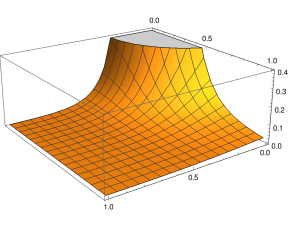
Figure 1: $k^{2}\mu$ of expression (42) for $(b=0,\>\>n=1,\>\>u=0.8\>)$

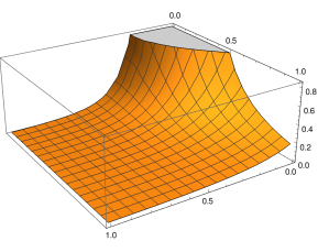
Figure 2: $k^{2}P_{\perp}$ of expression (43) for $(b=0,\>\>n=1,\>\>u=0.8\>)$

,

Figure 3: $k^{2}(\mu+P_{\perp})$ of expression (44) for $(b=0,\>\>n=1,\>\>u=0.8\>)$

3.2 Example 2

The solution with the $H(r)$ of Eq (48), which is given below

$$H(r)=-2Mk((1-b)e^{(r-k)/k}+br/k)$$ (48)

For the above $H(r)$ the expressions for $\mu$, $P_{\perp}$ and $\mu+P_{\perp}$ of Eqs (25), (27) and (29) in the variables $y$, $n$ and $u$ of Eqs (41) become

$$\mu=-\frac{1}{2\pi k^{2}\left(-2u^{2}x^{2}+4\sin(1-y)+\cos(2-2y)-3\right)^{2}}n(b(-e^{y-1})$$

$$+by+(b(-e^{y-1})+b+e^{y-1})\tan(1-y)+(b(e^{y-1}-1)-e^{y-1})$$

$$\sec(1-y)+e^{y-1})$$ (49)

$$P_{\perp}=-\frac{1}{64\pi k^{2}\left(u^{2}x^{2}+\sin^{2}(1-y)-2\sin(1-y)+1\right)^{2}}n(\sec^{3}(1-y)$$

$$(2(b-1)e^{y-1}\cos(1-y)(-2u^{2}x^{2}+4\sin(1-y)+\cos(2-2y)-3)+$$

$$(b(e^{y-1}-1)-e^{y-1})(2\sin(1-y)(2u^{2}x^{2}-3\cos(2-2y)+1)+$$

$$8\cos(2-2y))+8((1-b)e^{y-1}+by))$$ (50)

$$\mu+P_{\perp}=-\frac{1}{64\pi k^{2}\left(u^{2}x^{2}+(\sin(1-y)-2)\sin(1-y)+1\right)^{2}}n\sec^{3}(1-y)$$

$$(2(b-1)e^{y-1}\cos(1-y)(-2u^{2}x^{2}+4\sin(1-y)+\cos(2-2y)-3)-$$

$$(b(1-e^{y-1})+e^{y-1})(4u^{2}x^{2}\sin(1-y)-5\sin(3-3y)+3\sin(1-y)+$$

$$12\cos(2-2y)+4)+16((1-b)e^{y-1}+by)\cos^{3}(1-y))$$ (51)

Using numerical computer calculations we find that in the interior region $0\leq y\leq 1$ and $0\leq x^{2}\leq 1$ the following relations are satisfied:

$$\mu\geq 0,\>\>\>P_{\perp}\geq 0,\>\>\>\mu+P_{\perp}\geq 0\>\>\>\mbox{for}\>\>\>b\geq 1$$ (52)

Therefore the solution for $b\geq 1$ satisfies the WEC and the SEC. Also using numerical computer calculations we find that there is no value of $b$ for which $\mu-P_{\perp}\geq 0$ in the interior region. Therefore the solution does not satisfies the DEC.

According to our previous arguments the relation (21) should hold. For $F(r)$ and $H(r)$ given by Eqs (2) and (48) respectively and the use of Eqs (41) this relation becomes

$$u^{2}>n\left((1-b)e^{y-1}+by\right)-(1-\sin(1-y))^{2}$$ (53)

The graphs of $k^{2}\mu$, $k^{2}P_{\perp}$ and $k^{2}(\mu+P_{\perp})$ are presented in Figures (4), (5) and (6) for $b=2$, $n=1$ and $u=0.8$, which satisfy relation (53). With the help of a program [23] we can compute the minimum of these quantities for $0\leq y\leq 1$ and $0\leq x^{2}\leq 1$. We find the relations

$Mink^{2}\mu=0\>\>\>at\>\>\>y=1\>\>\>and\>\>\>x=3.38904*10^{-9}$

$Mink^{2}P_{\perp}=0.0121307,\>\>\>at\>\>\>y=1,\>\>\>and\>\>\>x=1$

$Mink^{2}(\mu+P_{\perp})=0.0121307,\>\>\>at\>\>\>y=1,\>\>\>and\>\>\>x=1$

in agreement with relations (52), which verify that the solution indeed satisfies the WEC and the SEC.

The line element of the solution is that of Eq (1) where $F(r)$ and $H(r)$ are given by Eqs (2) and (48) respectively.

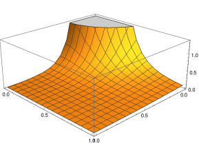
Figure 4: $k^{2}\mu$ of expression (49) for $(b=2,\>\>n=1,\>\>u=0.8\>)$

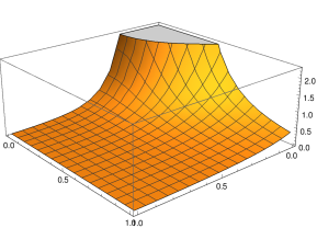
Figure 5: $k^{2}P_{\perp}$ of expression (50) for $(b=2,\>\>n=1,\>\>u=0.8\>)$

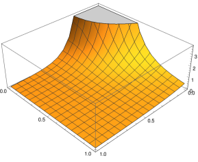
Figure 6: $k^{2}(\mu+P_{\perp})$ of expression (51) for $(b=2,\>\>n=1,\>\>u=0.8\>)$

3.3 Example 3

The solution with the $H(r)$ of Eq (54), which is given below

$$H(r)=-\frac{2M}{b}k^{1-b}\left((b-1)k^{b}+r^{b}\right)$$ (54)

For the above $H(r)$ the expressions for $\mu$, $P_{\perp}$ and $\mu+P_{\perp}$ of Eqs (25), (27) and (29) in the variables $y$, $n$ and $u$ of Eqs (41) become

$$\mu=-\frac{n(yt(y^{b}+b-1)+by^{b}\tan(1-y)-by^{b}\sec(1-y))}{2\pi bk^{2}y(-2u^{2}x^{2}+4\sin(1-y)+\cos(2-2y)-3)^{2}}$$ (55)

$$P_{\perp}=\frac{1}{32\pi k^{2}\left(u^{2}x^{2}+(\sin(1-y)-2)\sin(1-y)+1\right)^{2}}n(y^{b-2}\sec^{2}(1-y)$$

$$(-2bu^{2}x^{2}+4(b-1)\sin(1-y)+\cos(2-2y)(b-3y\tan(1-y)+$$

$$4y\sec(1-y)-1)-3b+2u^{2}x^{2}y\tan(1-y)+2u^{2}x^{2}+y\tan(1-y)+3)$$

$$-\frac{4(y^{b}+b-1)}{b})$$ (56)

$$\mu+P_{\perp}=-\frac{1}{64\pi k^{2}\left(u^{2}x^{2}+(\sin(1-y)-2)\sin(1-y)+1\right)^{2}}n\sec^{3}(1-y)$$

$$(-2(b-1)y^{b-2}\cos(1-y)(-2u^{2}x^{2}+4\sin(1-y)+\cos(2-2y)-3)-$$

$$y^{b-1}(4u^{2}x^{2}\sin(1-y)-5\sin(3-3y)+3\sin(1-y)+12\cos(2-2y)+4)$$

$$+\frac{16(y^{b}+b-1)\cos^{3}(1-y)}{b})$$ (57)

Using numerical computer calculations we find that in the interior region $0\leq y\leq 1$ and $0\leq x^{2}\leq 1$ the following relations are satisfied:

$$\mu\geq 0,\>\>\>P_{\perp}\geq 0,\>\>\>\mu+P_{\perp}\geq 0\>\>\>\mbox{for}\>\>\>0<b\leq 1$$ (58)

Therefore the solution for $0<b\leq 1$ satisfies the WEC and the SEC. Also using numerical computer calculations we find that there is no value of $b$ for which $\mu-P_{\perp}\geq 0$ in the interior region. Therefore the solution does not satisfies the DEC.

Also the relation (21) should hold. For $F(r)$ and $H(r)$ given by Eqs (2) and (54) respectively and the use of Eqs (41) this relation becomes

$$u^{2}>\frac{n}{b}\left(y^{b}+b-1\right)-(1-\sin(1-y))^{2}$$ (59)

The graphs of $k^{2}\mu$, $k^{2}P_{\perp}$ and $k^{2}(\mu+P_{\perp})$ are presented in Figures (7), (8) and (9) for $b=0.5$, $n=1$ and $u=0.8$, which satisfy relation (59). With the help of a program [23] we can compute the minimum of these quantities for $0\leq y\leq 1$ and $0\leq x^{2}\leq 1$. We find the relations

$Mink^{2}\mu=0\>\>\>at\>\>\>y=1\>\>\>and\>\>\>x=4.66932*10^{-8}$

$Mink^{2}P_{\perp}=0.00606536,\>\>\>at\>\>\>y=1,\>\>\>and\>\>\>x=1$

$Mink^{2}(\mu+P_{\perp})=0.00606536,\>\>\>at\>\>\>y=1,\>\>\>and\>\>\>x=1$

in agreement with relations (58), which verify that the solution indeed satisfies the WEC and the SEC.

The line element of the solution is that of Eq (1) where $F(r)$ and $H(r)$ are given by Eqs (2) and (54) respectively.

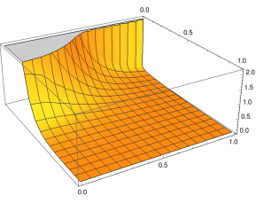
Figure 7: $k^{2}\mu$ of expression (55) for $(b=0.5,\>\>n=1,\>\>u=0.8\>)$

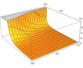
Figure 8: $k^{2}P_{\perp}$ of expression (56) for $(b=0.5,\>\>n=1,\>\>u=0.8\>)$

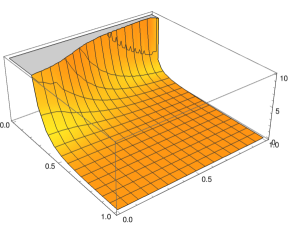
Figure 9: $k^{2}(\mu+P_{\perp})$ of expression (57) for $(b=0.5,\>\>n=1,\>\>u=0.8\>)$

3.4 Example 4

The solution with the $H(r)$ of Eq (60), which is given below

$$H(r)=-2M\left(bke^{\frac{r-k}{bk}}-bk+k\right)$$ (60)

For the above $H(r)$ the expressions for $\mu$, $P_{\perp}$ and $\mu+P_{\perp}$ of Eqs (25), (27) and (29) in the variables $y$, $n$ and $u$ of Eqs (41) become

$$\mu=\frac{n\left(b\left(-e^{\frac{y-1}{b}}\right)-e^{\frac{y-1}{b}}\tan(1-y)+e^{\frac{y-1}{b}}\sec(1-y)+b-1\right)}{8\pi k^{2}\left(u^{2}x^{2}+\sin^{2}(1-y)-2\sin(1-y)+1\right)^{2}}$$ (61)

$$P_{\perp}=\frac{1}{8\pi bk^{2}(-2u^{2}x^{2}+4\sin(1-y)+\cos(2-2y)-3)^{2}}n(\sec^{2}(1-y)$$

$$(b(2u^{2}x^{2}+1)\tan(1-y)+\cos(2-2y)(1-3b\tan(1-y))-2u^{2}x^{2}-3)$$

$$+4b(b(-e^{\frac{y-1}{b}})+b-1)+4b\cos(2-2y)\sec^{3}(1-y)+4\tan(1-y)$$

$$\sec(1-y))$$ (62)

$$\mu+P_{\perp}=\frac{1}{16\pi bk^{2}(-2u^{2}x^{2}+4\sin(1-y)+\cos(2-2y)-3)^{2}}n(e^{\frac{y-1}{b}}$$

$$\sec^{2}(1-y)(b(4u^{2}x^{2}+3)\tan(1-y)-4u^{2}x^{2}+2\cos(2-2y)-6)+16b$$

$$(b(-e^{\frac{y-1}{b}}+b-1)+8e^{\frac{y-1}{b}}\tan(1-y)\sec(1-y)+be^{\frac{y-1}{b}}\sec^{3}(1-y)(-5$$

$$\sin(3-3y)+12\cos(2-2y)+4))$$ (63)

With numerical computer calculations we find that in the interior region $0\leq y\leq 1$ and $0\leq x^{2}\leq 1$ the following relations are satisfied:

$$\mu\geq 0,\>\>\>P_{\perp}\geq 0,\>\>\>\mu+P_{\perp}\geq 0\>\>\>\mbox{for}\>\>\>b<0$$ (64)

Therefore the solution for $b<0$ satisfies the WEC and the SEC. Also with numerical computer calculations we find that there is no value of $b$ for which $\mu-P_{\perp}\geq 0$ in the interior region. Therefore the solution does not satisfies the DEC.

The relation (21), which should hold, becomes for $F(r)$ and $H(r)$ given by Eqs (2) and (60) respectively and the use of Eqs (41)

$$u^{2}>n\left(be^{\frac{y-1}{b}}-b+1\right)-((y-1)\sin+1)^{2}$$ (65)

The graphs of $k^{2}\mu$, $k^{2}P_{\perp}$ and $k^{2}(\mu+P_{\perp})$ are presented in Figures (10), (11) and (12) for $b=-1$, $n=1$ and $u=0.8$, which satisfy the above relation. With the help of a program [23] we can compute the minimum of these quantities for $0\leq y\leq 1$ and $0\leq x^{2}\leq 1$. We find the relations

$Mink^{2}\mu=0\>\>\>at\>\>\>y=1\>\>\>and\>\>\>x=2.36449*10^{-8}$

$Mink^{2}P_{\perp}=0.0121307,\>\>\>at\>\>\>y=1,\>\>\>and\>\>\>x=1$

$Mink^{2}(\mu+P_{\perp})=0.0121307,\>\>\>at\>\>\>y=1,\>\>\>and\>\>\>x=1$

in agreement with relations (64), which verify that the solution indeed satisfies the WEC and the SEC.

The line element of the solution is that of Eq (1) where $F(r)$ and $H(r)$ are given by Eqs (2) and (60) respectively.

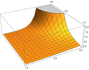
Figure 10: $k^{2}\mu$ of expression (61) for $(b=-1,\>\>n=1,\>\>u=0.8\>)$

Figure 11: $k^{2}P_{\perp}$ of expression (62) for $(b=-1,\>\>n=1,\>\>u=0.8\>)$

Figure 12: $k^{2}(\mu+P_{\perp})$ of expression (63) for $(b=-1,\>\>n=1,\>\>u=0.8\>)$

3.5 Example 5

The solution with the $H(r)$ of Eq (66), which is given below

$$H(r)=-\frac{2kM(br-k)}{(b-2)k+r}$$ (66)

For the above $H(r)$ the expressions for $\mu$, $P_{\perp}$ and $\mu+P_{\perp}$ of Eqs (25), (27) and (29) in the variables $y$, $n$ and $u$ of Eqs (41) become

$$\mu=-\frac{n}{2\pi k^{2}(b+y-2)^{2}(-2u^{2}x^{2}+4\sin(1-y)+\cos(2-2y)-3)^{2}}(b^{2}y+$$

$$by^{2}-2by+(b-1)^{2}\tan(1-y)+(b-1)^{2}(-\sec(1-y))-b-y+2)$$ (67)

$$P_{\perp}=\frac{n}{64\pi k^{2}(b+y-2)^{3}\left(u^{2}x^{2}+(\sin(1-y)-2)\sin(1-y)+1\right)^{2}}((b-1)^{2}$$

$$\sec^{3}(1-y)((b+y-2)(2\sin(1-y)(2u^{2}x^{2}-3\cos(2-2y)+1)+$$

$$8\cos(2-2y))-4\cos(1-y)(-2u^{2}x^{2}+4\sin(1-y)+\cos(2-2y)-3))+$$

$$8(b+y-2)^{2}(1-by))$$ (68)

$$\mu+P_{\perp}=\frac{n}{64\pi k^{2}(b+y-2)^{3}\left(u^{2}x^{2}+(\sin(1-y)-2)\sin(1-y)+1\right)^{2}}$$

$$\sec^{3}(1-y)-4(b-1)^{2}\cos(1-y)(-2u^{2}x^{2}+4\sin(1-y)+\cos(2-2y)$$

$$-3)+(b-1)^{2}(b+y-2)(4u^{2}x^{2}\sin(1-y)-5\sin(3-3y)+3\sin(1-y)$$

$$+12\cos(2-2y)+4)-16(b+y-2)^{2}(by-1)\cos^{3}(1-y))$$ (69)

With numerical computer calculations we find that in the interior region $0\leq y\leq 1$ and $0\leq x^{2}\leq 1$ the following relations are satisfied:

$$\mu\geq 0,\>\>\>P_{\perp}\geq 0,\>\>\>\mu+P_{\perp}\geq 0\>\>\>\mbox{for}\>\>\>b>2$$ (70)

which imply that the solution for $b>2$ satisfies the WEC and the SEC. Also with numerical computer calculations we find that there is no value of $b$ for which $\mu-P_{\perp}\geq 0$ in the interior region. Therefore the solution does not satisfies the DEC.

The relation (21), which should hold, becomes for $F(r)$ and $H(r)$ given by Eqs (2) and (66) respectively and the use of Eqs (41)

$$u^{2}>-\frac{n-bny}{b+y-2}-(1-\sin(1-y))^{2}$$ (71)

The graphs of $k^{2}\mu$, $k^{2}P_{\perp}$ and $k^{2}(\mu+P_{\perp})$ are presented in Figures (13), (14) and (15) for $b=3$, $n=1$ and $u=1.2$, which satisfy the above relation. With the help of a program [23] we can compute the minimum of these quantities for $0\leq y\leq 1$ and $0\leq x^{2}\leq 1$. We find the relations

$Mink^{2}\mu=0\>\>\>at\>\>\>y=1\>\>\>and\>\>\>x=8.62525*10^{-8}$

$Mink^{2}P_{\perp}=0.00815343,\>\>\>at\>\>\>y=1,\>\>\>and\>\>\>x=1$

$Mink^{2}(\mu+P_{\perp})=0.00815343,\>\>\>at\>\>\>y=1,\>\>\>and\>\>\>x=1$

in agreement with relations (70), which verify that the solution indeed satisfies the WEC and the SEC.

The line element of the solution is that of Eq (1) where $F(r)$ and $H(r)$ are given by Eqs (2) and (66) respectively.

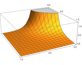
Figure 13: $k^{2}\mu$ of expression (67) for $(b=3,\>\>n=1,\>\>u=1.2\>)$

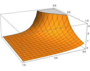
Figure 14: $k^{2}P_{\perp}$ of expression (68) for $(b=3,\>\>n=1,\>\>u=1.2\>)$

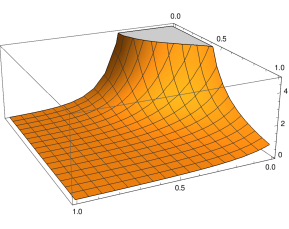
Figure 15: $k^{2}(\mu+P_{\perp})$ of expression (69) for $(b=3,\>\>n=1,\>\>u=1.2\>)$

References

- [1] Kerr R. P. Phys. Rev. Lett. 11, 237 (1963)
- [2] Krasinski A. Ann. Phys. 112, 22 (1978)
- [3] Des Mc Manus Class Quant. Grav. 8, 863 (1991)
- [4] Bicak J. and Ledvinka T. Phys. Rev. Lett. 71, 1669 (1993)
- [5] Pichon C. and Lynden-Bell D. Mon. Not. Roy. Astron. Soc. 280, 1007 (1996)
- [6] Viaggiu S. Int. J. Mod. Phys. D 15, 1441 (2006 )
- [7] Drake S. P. and Turolla R. Class. Quant. Grav. 14, 1883 (1997)
- [8] Kyriakopoulos E. Int. J. Mod. Phys. D 22, 1350051-1 (2013)
- [9] Hernandez-Pastora J. L. and Herrera L. Phys. Rev. D 95, 024003 (2017)
- [10] Herrera L. and Hernandez-Pastora J. L. Phys. Rev. D 96, 024048 (2017)
- [11] Ledvinka T. and Bicak J. Phys. Rev. D 99, 064046 (2019) arXiv : gr-gc /1903.01726v1.
- [12] Kyriakopoulos E. Interior Solutions to the Solution of Schwarzschild and to the Solution of Kerr (Lambert Academic Publishing, Beau Basin, 2021)
- [13] Boyer R. N. and Lindquist R. W. J. Math. Phys. 8, 265 (1967)
- [14] Torres R. and Fayos F. Gen. Rel. Grav. 49, 739 (2017)
- [15] Gurses M. and Gursey F. J. Math. Phys. 16, 2385 (1975)
- [16] Bonanos S: Riemannian Geometry and Tensor Calculus. In: Wolfram Research, Inc. Mathematica, Version 11.0, Champaign Il. (2016) www.inp.democritos.gr/ sbonano/RGTC/
- [17] Sakharov A. D. Sov. Phys. JETP 22, 241 (1966)
- [18] Gliner E. B. Sov. Phys. JETP 22, 378 (1966)
- [19] Ilic S. Kunz M. Liddle A. R. and Frieman J. A. Phys. Rev. D 81, 103502 (2010)
- [20] Mazur P. O. and Mottola E. Gravitational Condensate Stars: An Alternative to Black Holes (arXiv: gr-gc /0109035 )
- [21] Visser M. and Wiltshire D. L. Class. Quant. Grav. 21, 1135 (2004)
- [22] Herrera L. and Santos N. O. Phys. Rep. 286, 53 (1997)
- [23] To find global minima we use Wolfram’s programm [ NMinimize….] and [ NMaximize … ] for Numerical Nonlinear Global Optimization (Wolfram 2019).