Conditional Generative Model based Predicate-Aware Query Approximation

Abstract

The goal of Approximate Query Processing (AQP) is to provide very fast but “accurate enough” results for costly aggregate queries thereby improving user experience in interactive exploration of large datasets. Recently proposed Machine-Learning-based AQP techniques can provide very low latency as query execution only involves model inference as compared to traditional query processing on database clusters. However, with increase in the number of filtering predicates (WHERE clauses), the approximation error significantly increases for these methods. Analysts often use queries with a large number of predicates for insights discovery. Thus, maintaining low approximation error is important to prevent analysts from drawing misleading conclusions. In this paper, we propose Electra , a predicate-aware AQP system that can answer analytics-style queries with a large number of predicates with much smaller approximation errors. Electra uses a conditional generative model that learns the conditional distribution of the data and at run-time generates a small ($\approx$ 1000 rows) but representative sample, on which the query is executed to compute the approximate result. Our evaluations with four different baselines on three real-world datasets show that Electra provides lower AQP error for large number of predicates compared to baselines.

1 Introduction

Interactive exploration and visualization tools, such as Tableau, Microsoft Power BI, Qlik, Polaris (Stolte, Tang, and Hanrahan 2002), and Vizdom (Crotty et al. 2015) have gained popularity amongst data-analysts. One of the desirable properties of these tools is that the speed of interaction with the data, i.e., the queries and the corresponding visualizations must complete at “human speed”  (Crotty et al. 2016) or at “rates resonant with the pace of human thought” (Liu and Heer 2014).

To reduce the latency of such interactions, Approximate Query Processing (AQP) techniques that can provide fast but “accurate enough” results for queries with aggregates (AVG, SUM, COUNT) on numerical attributes on a large dataset, have recently gained popularity (Hilprecht et al. 2020; Thirumuruganathan et al. 2020; Ma and Triantafillou 2019). Prior AQP systems mainly relied on sampling-based methods. For example, BlinkDB (Agarwal et al. 2013) and recently proposed VerdictDB (Park et al. 2018b), first create uniform/stratified samples and store them. Then at run-time, they execute the queries against these stored samples thus reducing query latency. In order to reduce error for different set of queries — using different columns for filters and groupings — they need to create not one, but multiple sets of stratified samples of the same dataset. This results in a significant storage overhead. Recently, following the promising results (Mondal, Sheoran, and Mitra 2021; Mirhoseini et al. 2017; Kraska et al. 2018) of using Machine Learning (ML) to solve several systems problems, few ML-based AQP techniques have been proposed. These use either special data-structures (DeepDB (Hilprecht et al. 2020)) or simple generative models (VAE-AQP (Thirumuruganathan et al. 2020)) to answer queries with lower latency.

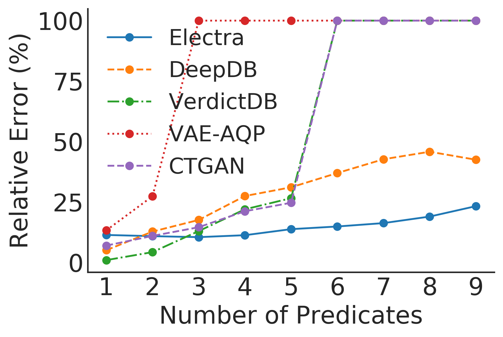
Figure 1: Median relative error vs. no. of predicates. Baselines have high error for important high-predicate queries.

However, a key drawback of these techniques is that as the number of predicates (i.e. WHERE conditions) in the query increases, the approximation error significantly increases (Fig. 1 for Flights dataset). Electra is our technique shown in blue. The importance of the queries containing such large number of predicates is disproportionally high. This is because, as expert analysts drill down for insights, they progressively use more and more predicates to filter the data to arrive at the desired subset and breakdowns where some interesting patterns might be present. Therefore, lowering the approximation error for such high-predicate queries can prevent wrong conclusions, after laborious dissection of data in search of insights. As shown in Fig. 1, all baselines fail to achieve this goal and therefore can be detrimental for complex insight discovery tasks.

In this paper, we present Electra, a predicate-aware AQP system that can answer analytics-style queries having a large number of predicates with much lower approximation errors compared to the state-of-the-art techniques. The key novelty of Electra comes from the use of a predicate-aware generative model for AQP and associated training methodology to capture accurate conditional distribution of the data even for highly selective queries. Electra then uses the conditional generative model (Sohn, Lee, and Yan 2015) to generate a few representative samples at runtime for providing an accurate enough answer.

The attributes (columns) in a tabular dataset can have categories (groups) that are rare. Moreover, when a large number of predicates are used to filter the data, the number of rows in the original data satisfying such conditions can be very small. If we cannot faithfully generate such rare categories with proper statistical characteristics, AQP results would either have large errors or even miss entire groups for queries using a GROUP BY. To overcome this problem, we propose a stratified masking strategy while training the CVAE and an associated modification of the CVAE loss-function to help it learn predicate-aware targeted generation of samples. Specifically, using this proposed masking strategy, we help the model to learn rare groups or categories in the data. Our empirical evaluations on real-world datasets show that, our stratified masking strategy helps Electra to learn the conditional distribution among different attributes, in a query-agnostic manner and can provide an average 12% improvement in accuracy (Fig. 8) compared to random masking strategy proposed by prior work (Ivanov, Figurnov, and Vetrov 2019) (albeit, not for AQP systems but for image generation). Our major contributions in this paper are:

• We propose a novel and low-error approximate query processing technique using predicate-aware generative models. Even for queries with a large number of predicates, our technique can provide effective answers by generating a few representative samples, at the client-side.

• We propose a novel stratified-masking technique that enables training the generative model to learn better conditional distribution and support predicate-aware AQP resulting in a significant performance improvement on low selectivity queries.

• We present the end-to-end design and implementation details of our AQP system called Electra. We present detailed evaluation and ablation study with real-world datasets and compare with state-of-the-art baselines. Our technique reduces AQP error by 36.6% on average compared to previously proposed generative-model-based AQP technique on production workloads.

2 Overview of Electra

Target Query Structure

The commonly used queries for interactive data exploration and visual analytics have the following structure:
SELECT $\Psi$, AGG($N$) as $\alpha$ FROM $T$ WHERE $\theta$ [GROUP BY $C$] [ORDER BY $\beta$]

Aggregate AGG (AVG, SUM etc.) is applied to a numerical attribute $N$, on rows satisfying predicate $\theta$. GROUP BY is optionally applied on categorical attributes $C$. One such query example is shown in Fig. 2(b). Here an analyst might be exploring what are the average checkout values made by users from a certain demographic (Age “Senior” using “iOS” and “Chrome” Browser) from an e-commerce site across different months. Insights like these helps organizations to understand trends, optimize website performance or to place effective advertisements. Electra can handle a much diverse set of queries including queries with multiple predicates by - breaking down the query into multiple queries; using inclusion-exclusion principle or converting the query’s predicates to Disjunctive Normal Form. For more details, please refer to the supplement section Query Handling.

Predicates: Predicates are condition expressions (e.g., WHERE) evaluating to a boolean value used to filter rows on which an aggregate function like AVG, SUM and COUNT is to be evaluated. A compound predicate consists of multiple (ANDs) or (ORs) of predicates.

Query Selectivity: The selectivity of a query with predicate $\pi$ is defined as $sel\left(\pi\right)\coloneqq\lvert{x\in T\colon\pi\left(x\right)=1}\rvert/\lvert{T}\rvert$. It indicates what fraction of rows passed the filtering criteria used in the predicates.

Design of Electra

Fig. 2(a) shows the major components of Electra (marked in green). At a high-level, it has primarily two components: an on-line AQP runtime at the client-side and, an offline server-side ETL (Extraction, Transformation, and Loading) component. The runtime component is responsible for answering the live queries from the user-interactions using the pre-trained ML-models. It pulls these models asynchronously from a repository (Model-DB) and caches them locally. Electra is designed to handle the most frequent-type of queries for exploratory data analytics (Refer § 2). Unsupported query-formats are redirected to a backend query-processor.

Fig. 2(b) shows more details of the runtime component. Electra first parses the query to extract individual predicates, GROUP BY attributes, and the aggregate function. If the aggregate is either a SUM or an AVG, Electra feeds the predicates and the GROUP BY information to its predicate-aware ML-model ( ) and generates a small number of representative samples. For queries with AVG as an aggregate, Electra can directly calculate the result by applying the query logic on these generated samples ( ). For SUM queries, Electra needs to calibrate the result using an appropriate scale-up or denormalizing factor. Electra calculates this factor by feeding the filtering predicates to a selectivity estimator ( ). For COUNT queries, Electra directly uses the selectivity estimator to calculate the query result.

The server-side ETL component ( in Fig. 2(a)) operates asynchronously. For a new dataset, it trains two types of models – a conditional generative model and a selectivity estimator model – and stores them into the Model-DB.

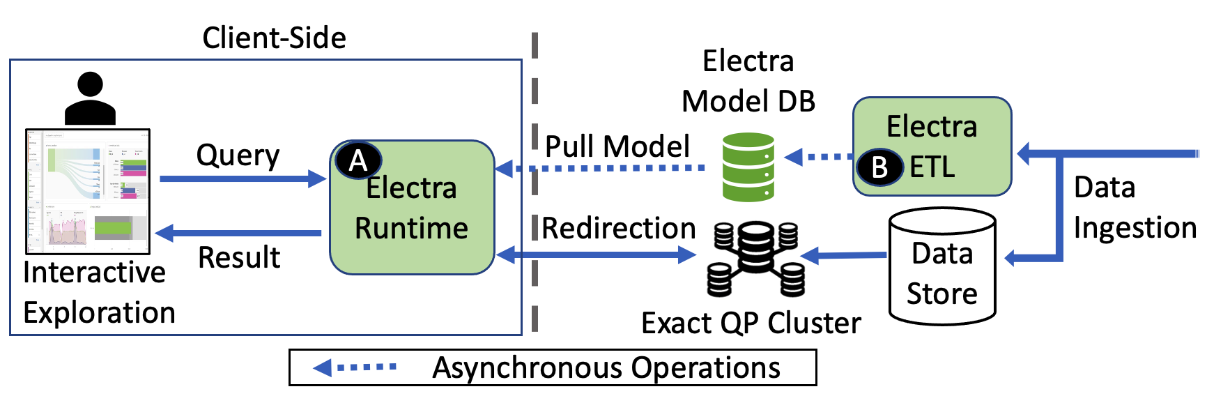
(a) Overall architecture of Electra

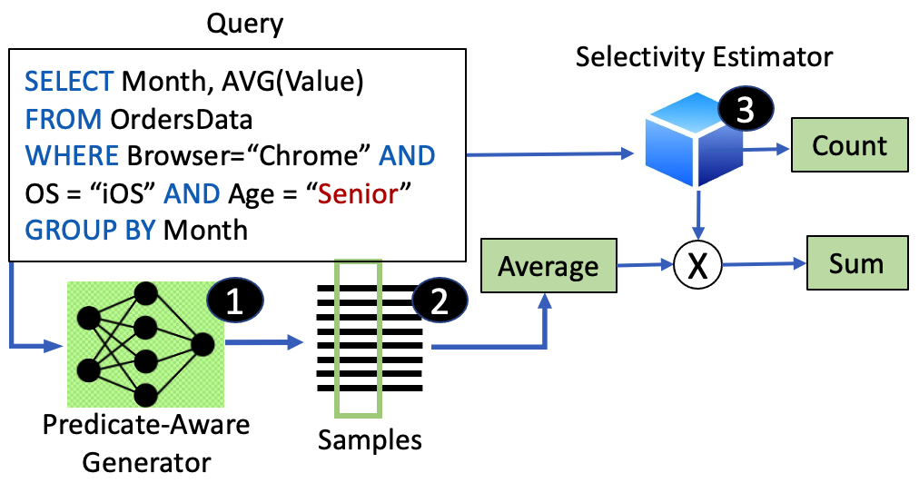
(b) Electra Runtime computations

Figure 2: Design of Electra

3 Conditional Sample Generation

In this section, we describe how Electra attempts to make conditional sample generation process accurate, even for queries with large number of predicates, so that the resulting approximation error on these samples becomes very small.

Problem Description

Let T be a relation with $K=|A|$ attributes where $A=A_{N}\cup A_{C}$. $A_{N}$ denotes the numerical attributes and $A_{C}$ denotes the categorical attributes. Our aim is to learn a model that can generate a predicate-aware representative sample of T at runtime. This problem can be divided into two sub-problems – first, learning the conditional distributions of the form $P(A_{n}|A_{c})$ where $A_{n}$ is a subset of $A_{N}$ and $A_{c}$ is a subset of $A_{C}$ and second, generating representative samples using the learned conditional distributions. With respect to the example query in Fig. 2(b), the attribute Value belongs to $A_{N}$. The attributes Browser, OS, Age and Month used in the predicates are categorical attributes and belongs to $A_{C}$.

Electra targets to support queries with arbitrary number of predicate combinations over the attributes $A_{C}$ using only a single model. This requires the learning technique to be query-agnostic (but yet, sample generation to be query-predicate specific).

Electra’s Model Design

We are the first to propose the use of Conditional Variational Auto-encoders (CVAE) (Sohn, Lee, and Yan 2015) along with a query-agnostic training methodology involving a novel masking strategy to reduce the AQP error.

Consider a $K$-dimensional vector $a$ with numerical and categorical values representing a row of data. Let $m\in{\{0,1\}}^{K}$ be a binary mask denoting the set of unobserved ($m_{i}=1$) and observed attributes ($m_{i}=0$). Applying this mask on the vector $a$ gives us $a_{m}=\{a_{i:m_{i}=1}\}$ as the set of unobserved attributes and $a_{1-m}=\{a_{i:m_{i}=0}\}$ as the set of observed attributes. Our goal is to model the conditional distribution of the unobserved $a_{m}$ given the mask $m$ and the observed attributes $a_{1-m}$ i.e. approximate the true distribution $p(a_{m}|a_{1-m},m)$.

Along with providing full support over the domain of $m$ (arbitrary conditions), we need to ensure that the samples that are generated represent rows from the original dataset. For example: given a set of observed attributes $a_{1-m}$ whose combination does not exist in the data, the model should not generate samples of data satisfying $a_{1-m}$ (since a false positive). To avoid this, we learn to generate complete $a$ (both $a_{m}$ and $a_{1-m}$) by learning the distribution $p(a|a_{1-m},m)$ instead of just learning $p(a_{m}|a_{1-m},m)$ and hence avoiding generating false positives.

Note that the generative models based on VAE(s) (Kingma and Welling 2014) allows us to generate random samples by generating latent vector $z$ and then sampling from posterior $p_{\theta}(x|z)$. But, we do not have any control on the data generation process. Conditional Variational Auto-encoder models (CVAE) (Sohn, Lee, and Yan 2015) counter this by conditioning the latent variable and data generation on a control variable. In terms of the table attributes $a$, the control variable $a_{1-m}$ and the mask $m$, the training objective for our model thus becomes:

$$\mathcal{L_{\text{{\sc Electra}}}}=-KL(q_{\phi}(z|a,m)||p_{\psi}(z|a_{1-m},m))+\\ \mathbb{E}_{z\sim q_{\phi}(z|a,m)}[log(p_{\theta}(a|z))]$$ (1)

The loss function is a combination of two terms: (1) KL-divergence of the posterior and the conditional distribution of the latent space i.e. how well is your conditional latent space generation and (2) Reconstruction error for the attributes i.e. how well is your actual sample generation.

The generative process of our model thus becomes: (1) generate latent vector conditioned on the mask and the observed attributes: $p_{\psi}(z|a_{1-m},m)$ and (2) generate sample vector $a$ from the latent variable $z$: $p_{\theta}(a|z)$, thus inducing the following distribution:

$$p_{\psi,\theta}(a|a_{1-m},m)=\mathbb{E}_{z\sim p_{\psi}(z|a_{1-m},m)}p_{\theta}(a|z)$$ (2)

Since $a_{m}$ and $a_{1-m}$ can be variable length vectors depending on $m$, inspired from (Ivanov, Figurnov, and Vetrov 2019), we consider $a_{m}=a\circ m$ i.e. the element-wise product of $a$ and $m$. Similarly, $a_{1-m}=a\circ(1-m)$.

In terms of a query, the observed attributes are the predicates present in the query. E.g. for the query in Fig. 2(b), for attributes $A$ = {Month, Value, Browser, OS, Age}, $m$ is $\{1,1,0,0,0\}$ and the observed attributes vector $a_{1-m}$ is {-, -, "Chrome", "iOS", "Senior"}.

Model Architecture:

Electra’s CVAE model consists of three networks - (1) Encoder: to approximate the true posterior distribution, (2) Prior: to approximate the conditional latent space distribution, and (3) Decoder: to generate synthetic samples based on the latent vector $z$. We use a Gaussian distribution over $z$ with parameters $(\mu_{\phi},\sigma_{\phi})$ and $(\mu_{\psi},\sigma_{\psi})$ for the encoder and prior network respectively. Fig. 3(a) shows the model architecture. All the three networks are used during training, whereas during runtime, only the prior and decoder networks are used. Fig. 3(b) shows the inputs to these networks during training, corresponding to our example dataset mentioned in Fig. 2(b). The input to the Prior network is masked using a novel masking strategy. Fig. 3(c) illustrates the runtime inputs to Electra’s generative model for our example query. It also illustrates the generated samples as obtained from the Decoder network, corresponding to the input query. After generation of such targeted samples that preserve the conditional distribution of the original data in the context of the query received at runtime, Electra simply executes the original query on this very small sample to calculate an answer.

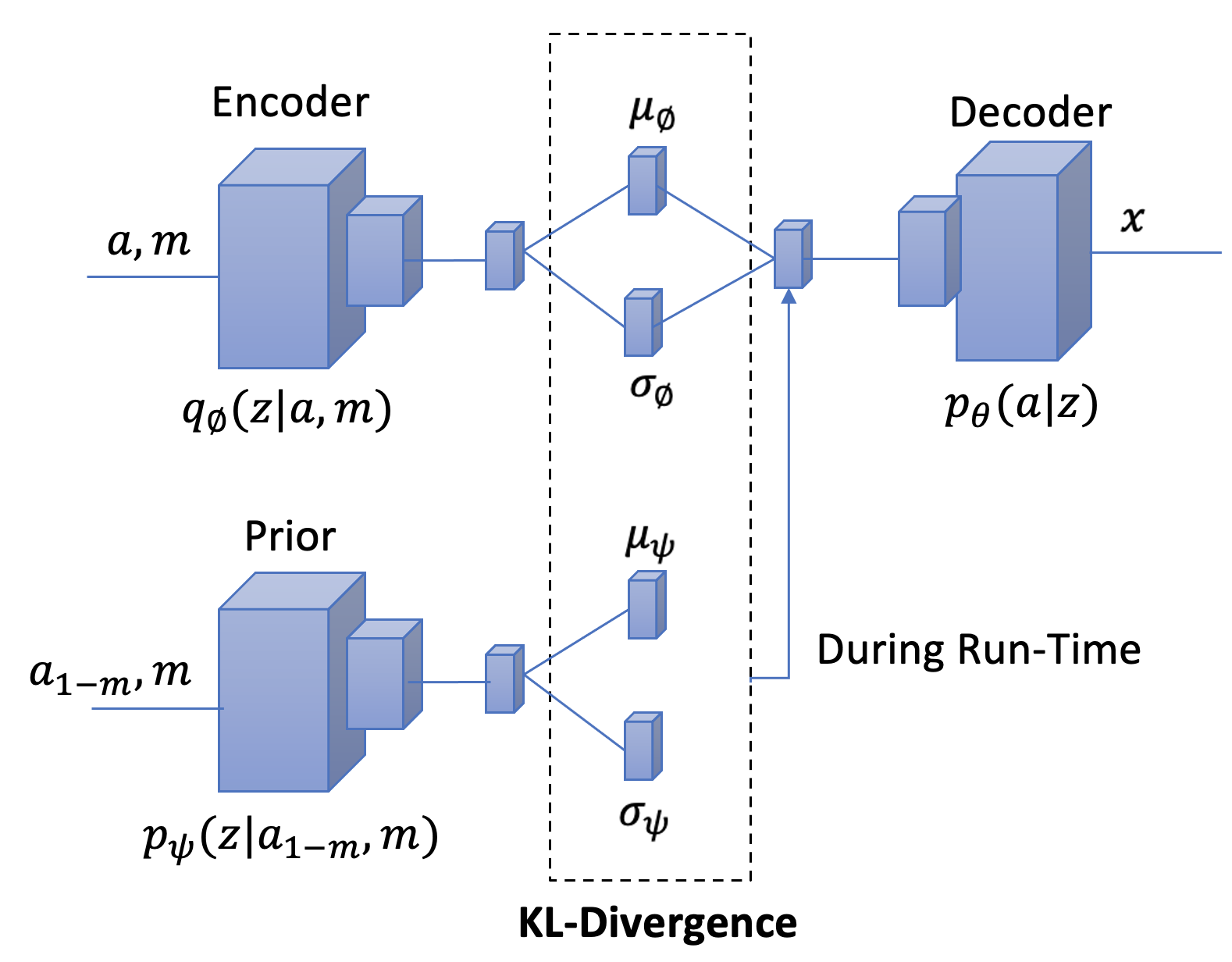
(a) Model architecture

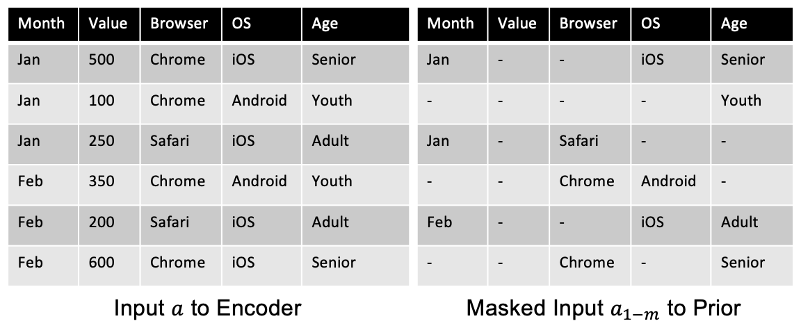
(b) Training inputs

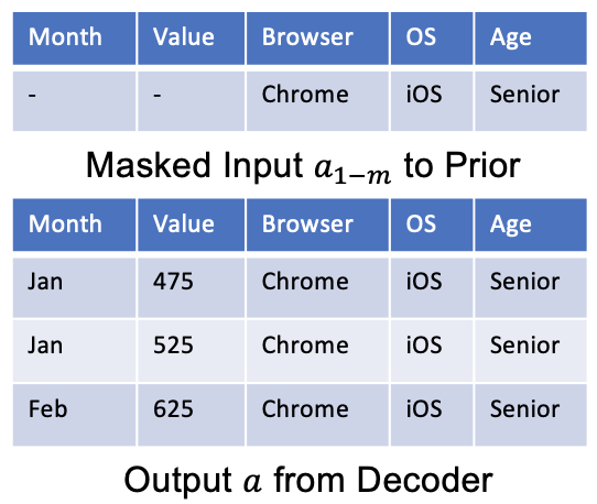
(c) Runtime inputs

Figure 3: Model architecture and inputs

Stratified Masking

The efficiency of learned conditional distributions depends on the set of masks $M=\{m\}$ used during the training. During each epoch, a mask $m_{b\times k}$ is generated for a batch of data. This mask is applied to the input data to generate the set of observed attributes, for which the samples are generated and the loss function evaluated. In case of $m={0}^{K}$ i.e. no masking and all the attributes are observed, the prior network would learn to generate latent vectors corresponding to all observed attributes. But at runtime, only a partial set of attributes are observed (as predicates) and hence it would lead to a poor performance. In case of $m={1}^{K}$ i.e. a masking rate of 100% and all the features are unobserved, the behavior would be similar to that of a VAE. Since the vector $a_{1-m}=\{\phi\}$, the conditioning of the latent vector would have no effect on the learning. Thus, again this would perform poorly on queries with predicates.

In order to counter these and make the training query-agnostic, a random masking strategy (Ivanov, Figurnov, and Vetrov 2019) can be used where a certain fraction of the rows are masked corresponding to each of the input features. However, such random masking does not provide any mechanism to help the model learn better the conditional distribution for rare groups to improve performance for queries with large number of predicates. There are more subtleties. By masking more number of rows for an attribute, the training helps the model to learn better the generation of representative values for that attribute. Whereas, by keeping more unmasked rows, the model can learn better conditional distribution conditioned on those attributes.

Input: Batch $\{B\}_{b\times k}$, Masking Factor $r$, Strata Size $S$

Output: Binary mask $m$ for the Input Batch $B$

1 $m\leftarrow{0}_{b\times k}$

2 $num\_cols\leftarrow numerical\_cols(k)$

3 $cat\_cols\leftarrow categorical\_cols(k)$

4 for $i$ in $num\_cols$ do

5       $\{m_{x,y}\}_{1,i}^{b,i}\leftarrow 1$

6      

7 end for

8for $i\in cat\_cols$ do

9       $values\leftarrow\{B_{x,y}\}_{1,i}^{b,i}$

10       $weights\leftarrow\{S_{i}[values_{x}]\}_{1}^{b}$

11       $batch\_indices\leftarrow random.sample(\{x\}_{1}^{b},r*b,weights)$

12       for $j\in batch\_indices$ do

13             $m_{j,i}\leftarrow 1$

14            

15       end for

16      

17 end for

return $m;$

Algorithm 1 Stratified Masking Strategy

Proposed masking strategy: With the above observation, Electra uses a novel masking strategy tailored for AQP. It consists of the following: (a) We completely mask the numerical attributes. (b) For the categorical attributes on which conditions can be used in the predicates, we use a stratified masking strategy. In the stratified masking we alter the random masking strategy based on the size of the strata (i.e. groups or categories) to disproportionately reduce the probability of masking for the rare groups. Thus, the ability of the model to learn better conditional distribution improves. We apply this masking strategy in a batch-wise manner during training. In the Evaluation section, we show (Fig. 8) that our masking strategy drastically reduces the approximation error compared to no-masking or random masking strategies.

Algorithm 1 describes the masking strategy where we input a batch of data $B$ of dimension $b\times k$: $b$ denotes the batch size and $k$ denotes the number of attributes. The numerical columns are completely masked. The strata size for each categorical column $i$ ($S_{i}$), contains for each value that the column $i$ can take, the fraction of rows in the data where the column takes this value. Using the $weights$ obtained from $S_{i}[value]$ as the sampling probability and $r$ as the masking factor, we sample $r*b$ rows and mask their column $i$. Masking factor $r$ controls the overall masking rate of the batch. A higher masking factor simulates queries with less observed attributes i.e. less number of predicates and a lower masking factor simulates queries with more observed attributes i.e. more number of predicates.

4 Implementation Details

Data Transformation. Electra applies a set of data pre-processing steps including label encoding for categorical attributes and mode-specific normalization for numerical attributes. For normalization, weights for the Gaussian mixture are calculated through a variational inference algorithm using sklearn’s BayesianGaussianMixture method. The parameters specified are the number of modes (identified earlier) and a maximum iteration of 1000. To avoid mixture components with close to zero weights, we limit the number of modes to less than or equal to 3.

Conditional Density Estimator. The conditional density estimator model is implemented in PyTorch. We build upon the code  provided by Ivanov et al. The density estimator is trained to minimize the combination of KL-divergence loss and reconstruction loss. To select a suitable set of hyperparameters, we performed a grid search. We varied the depth ($d$) of the prior and proposal networks in the range [2,4,6,8] and the latent dimension ($L$) in the range [32,64,128,256]. For Flights data we use $d=8$, $L=64$, for Housing $d=8$, $L=64$, and for Beijing PM2.5 we use $d=6$, $L=32$. Note that, the depth of the networks and the latent dimension contribute significantly to the model size. Hence, depending on the size constraints (if any), one can choose a simpler model. We used a masking factor ($r$) of 0.5. The model was trained with an Adam Optimizer with a learning rate of 0.0001 (larger learning rates gave unstable variational lower bound(s)).

Selectivity Estimator. We use Naru’s publicly available implementation . The model is trained with the ResMADE architecture with a batch size of 512, an initial warm-up of 10000 rounds, with 5 layers each of hidden dimension 256. In order to account for the impact of column ordering, we tried various different random orderings and chose the one with the best performance.

We provide more details about the pre-processing steps and training methodology in the supplement section: Implementation Details.

5 Evaluation

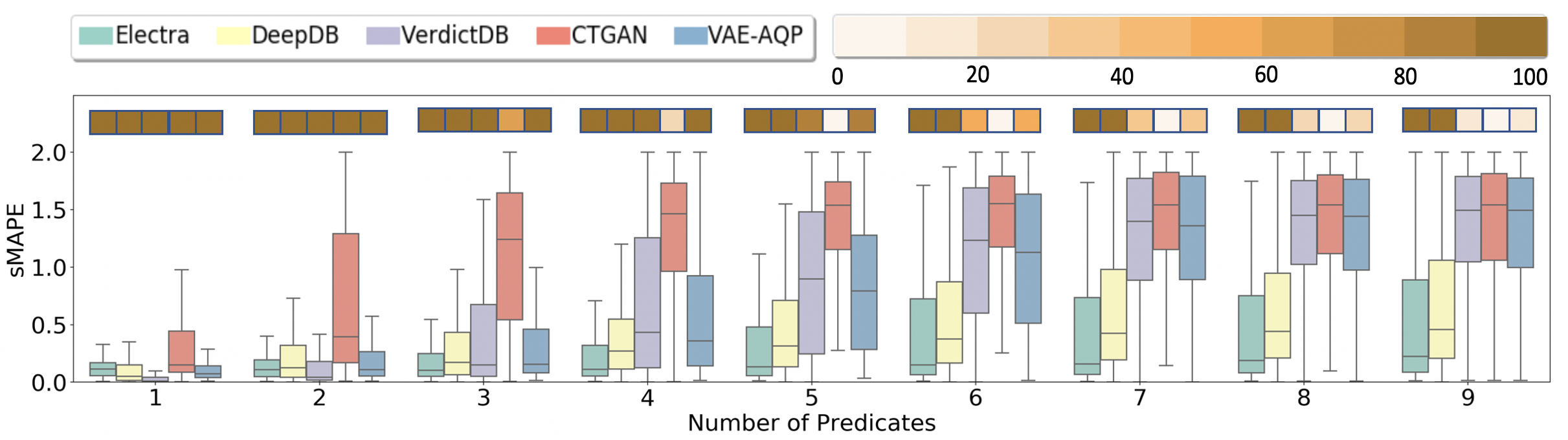
(a) Flights

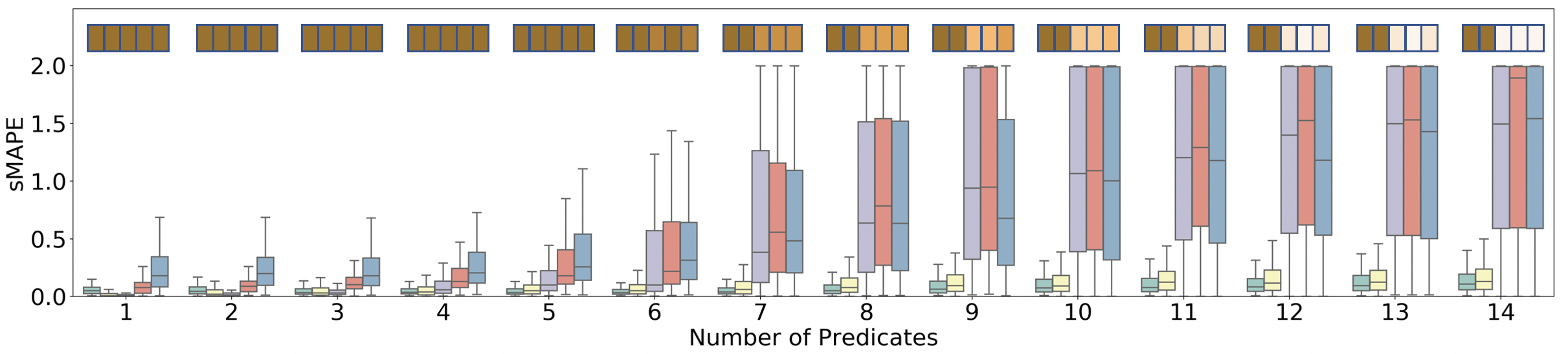
(b) Housing

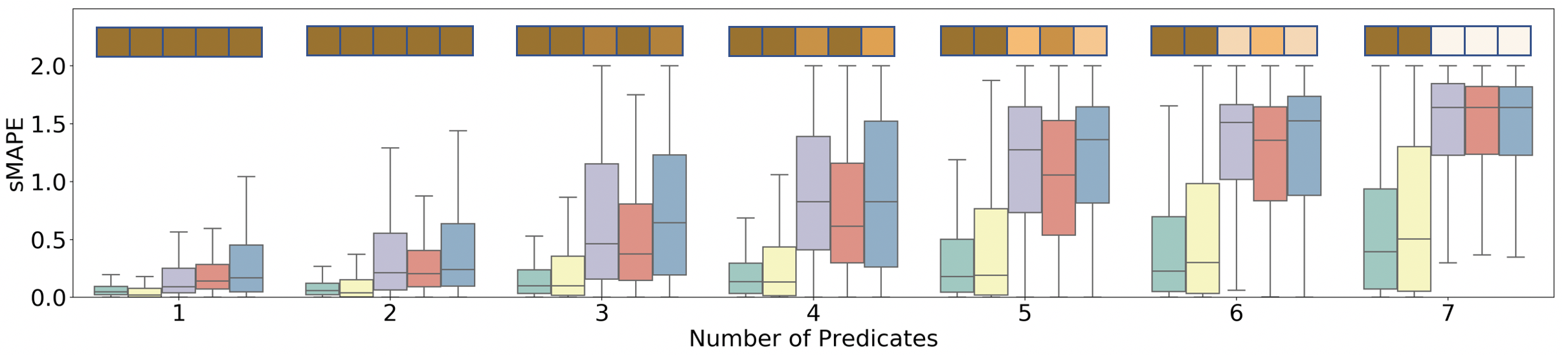
(c) Beijing PM2.5

Figure 4: AQP error vs. # predicates. Heat-map shows % of queries answered.

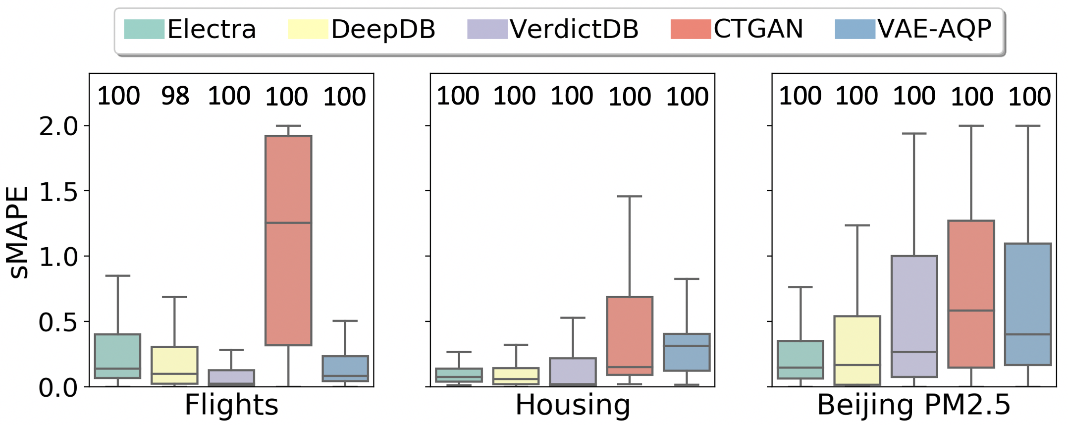
(d) AVG queries

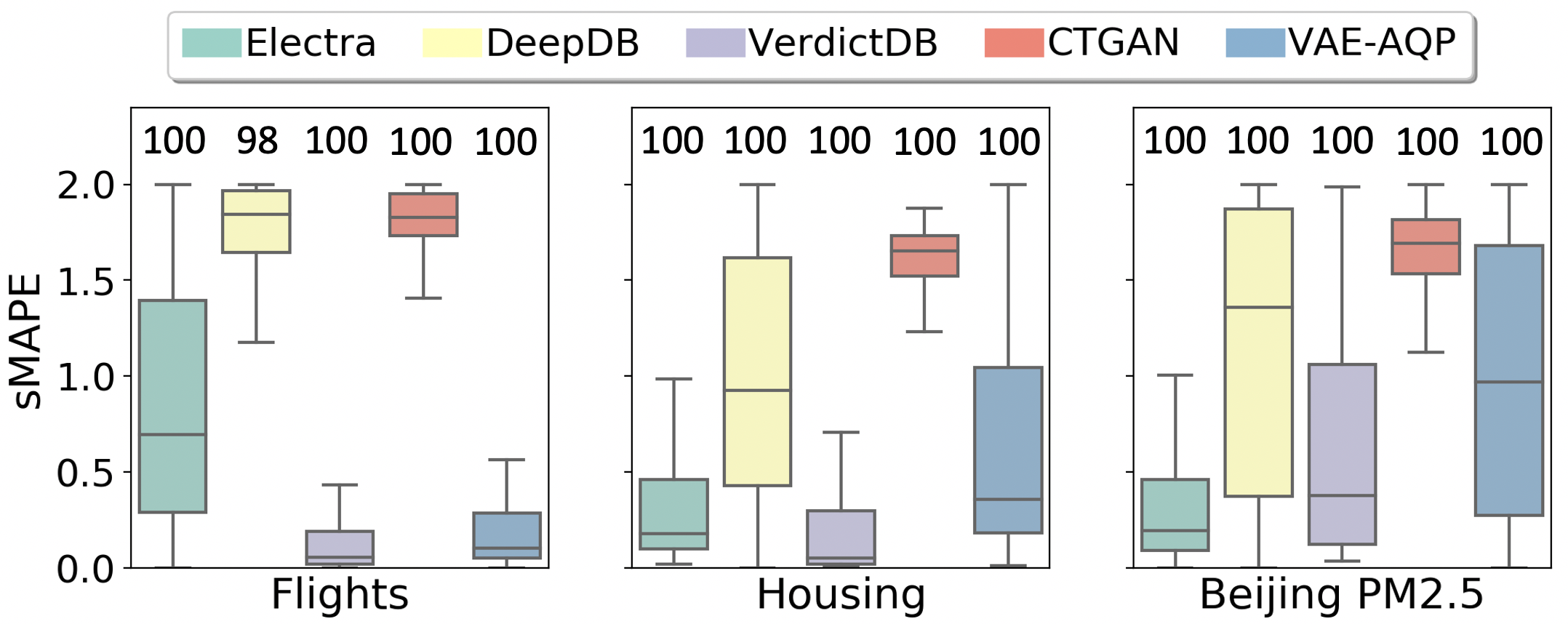
(e) SUM queries

Figure 5: AQP error vs. # predicates. number on top shows % of queries answered.

Dataset	Sample size
	500	1000	1500	2000
Flights	15.15	14.93	14.70	14.60
Housing	5.96	5.91	5.92	5.92
Beijing PM2.5	15.98	15.79	15.77	15.64

Table 1: Median R.E. vs. # samples generated

Experimental Environment

All the experiments were performed on a 32 core Intel(R) Xeon(R) CPU E5-2686 with 4 Tesla V100-SXM2 GPU(s).

Datasets: We use three real-world datasets: Flights (of Transportation Statistics 2019), Housing (Qiu 2018) and Beijing PM2.5 (Chen 2017). The Flights dataset consists of arrival and departure data (e.g. carrier, origin, destination, delay) for domestic flights in the USA. The Housing dataset consists of housing price records (e.g. price, area, rooms) obtained from a real-estate company. The Beijing PM2.5 dataset consists of hourly records of PM2.5 concentration. All these datasets have a combination of both categorical and numerical attributes. (Ref. Supplement Table 1).

Synthetic Query Workload: We create a synthetic workload to evaluate the impact of the number of predicates in the query. For each dataset, we generated queries with # of predicates ($k$) ranging from 1 to $|A_{C}|$. For a given $k$, we first randomly sample 100 combinations (with repetitions) from the set of all possible $k$-attribute selections. Then, for each of these selected $k$-attributes, we create the WHERE condition by assigning values based on a randomly chosen tuple from the dataset. Then, we use AVG as the aggregate function for each of the numerical attributes. The synthetic workload thus contains a total of $100*|A_{C}|*|A_{N}|$ queries.

Production Query Workload: We also evaluate Electra using real production queries from five Fortune 500 companies over a period of two months on a large data exploration platform. First, we select queries whose query structure is supported by Electra. We filter out the repeated queries. While we were able to extract the queries, we did not have access to the actual customer data corresponding to those queries. Hence, we use the following methodology to create an equivalent query set for our evaluation. We replace each predicate in the WHERE clause by a random categorical attribute and a random value corresponding to that attribute. All attributes that were used in GROUP BY were replaced by random categorical attributes from our evaluation datasets. Then, we generate two workloads, one with AVG and one with SUM as the aggregate function on a random numerical attribute. Thus, we preserve real characteristics of the use of predicates and the grouping logic in our modified workload. For details on the query selectivity, please refer to the supplement.

Baselines:

We evaluate against four recent baselines.

VAE-AQP (Thirumuruganathan et al. 2020) is a generative model-based technique that does not use any predicate information. The code was obtained from the authors. In our evaluations, we generated 100K samples from VAE-AQP for all 3 datasets. Note that this is well over the $1\%$ sampling rate specified by the VAE-AQP authors for these datasets.

CTGAN (Xu et al. 2019) is a conditional generative model. However, the CTGAN technique as described in the paper  (Xu et al. 2019) and the associated code (CTGAN code ), only support at most one condition for generation. Hence, when using CTGAN as a baseline in our evaluation, we randomly select one of the input predicates as the condition for generating the samples. We keep the generated sample size per query same as Electra.

DeepDB (Hilprecht et al. 2020) builds a relational sum-product-network (SPN) based on the input data. For any incoming query, it evaluates the query on the obtained SPN network. We keep the default parameters for DeepDB code obtained from (DeepDB code ).

VerdictDB (Park et al. 2018b) is a sampling-based approach that runs at the server-side. It extracts and stores samples (called SCRAMBLE) from the original data and uses it to answer the incoming queries. We keep the default parameters in the code obtained from (VerdictDB code ).

AQP Error Measures:

For a query $Q$, with an exact ground truth result $g$ and an approximate result $a$, we measure the approximation error by computing the Relative Error (R.E.).

Since R.E. is an unbounded measure and can become very large, we use a bounded measure called Symmetric Mean Absolute Percentage Error (sMAPE) to visualize the approximation errors. sMAPE lies between 0 and 2 and provides a better visualization compared to R.E..

$$\textit{sMAPE}(Q)=2*\frac{|g-a|}{|g|+|a|}$$

Performance w.r.t. Number of Predicates

Fig. 5 shows the distribution of approximation error (as sMAPE) w.r.t. the number of predicates in the synthetic workload queries. A lower approximation error is better. All the queries could not be successfully evaluated to produce an approximate result because the technique could not match for the used predicates either in the generated data (Electra, CTGAN, VAE-AQP) or in the available samples (VerdictDB) or in the stored metadata (DeepDB). The distribution of the AQP errors in the box-plots were calculated only over the queries that the corresponding technique could support. The heat-map colors over the box-plots show what percentages of the queries were supported by different techniques. A technique supporting large fraction of queries is better. It is worthwhile to note, only Electra and DeepDB could answer the queries with $90-100\%$ coverage across all the different predicate settings.

Note, the median approximation error is almost always the lowest for Electra (shown in green), as the number of predicates in the queries are increased. The other two generative baselines, CTGAN and VAE-AQP perform poorly in this aspect. DeepDB’s performance is great for median approximation comparison, but error at the tail is often quite large for DeepDB, compared to Electra. For one predicate, almost all the techniques can maintain very low AQP error (making any of those practically useful) and Electra often does not provide the lowest error in the relative terms. However, Electra is the overall best solution when we look at the whole spectrum of predicates.

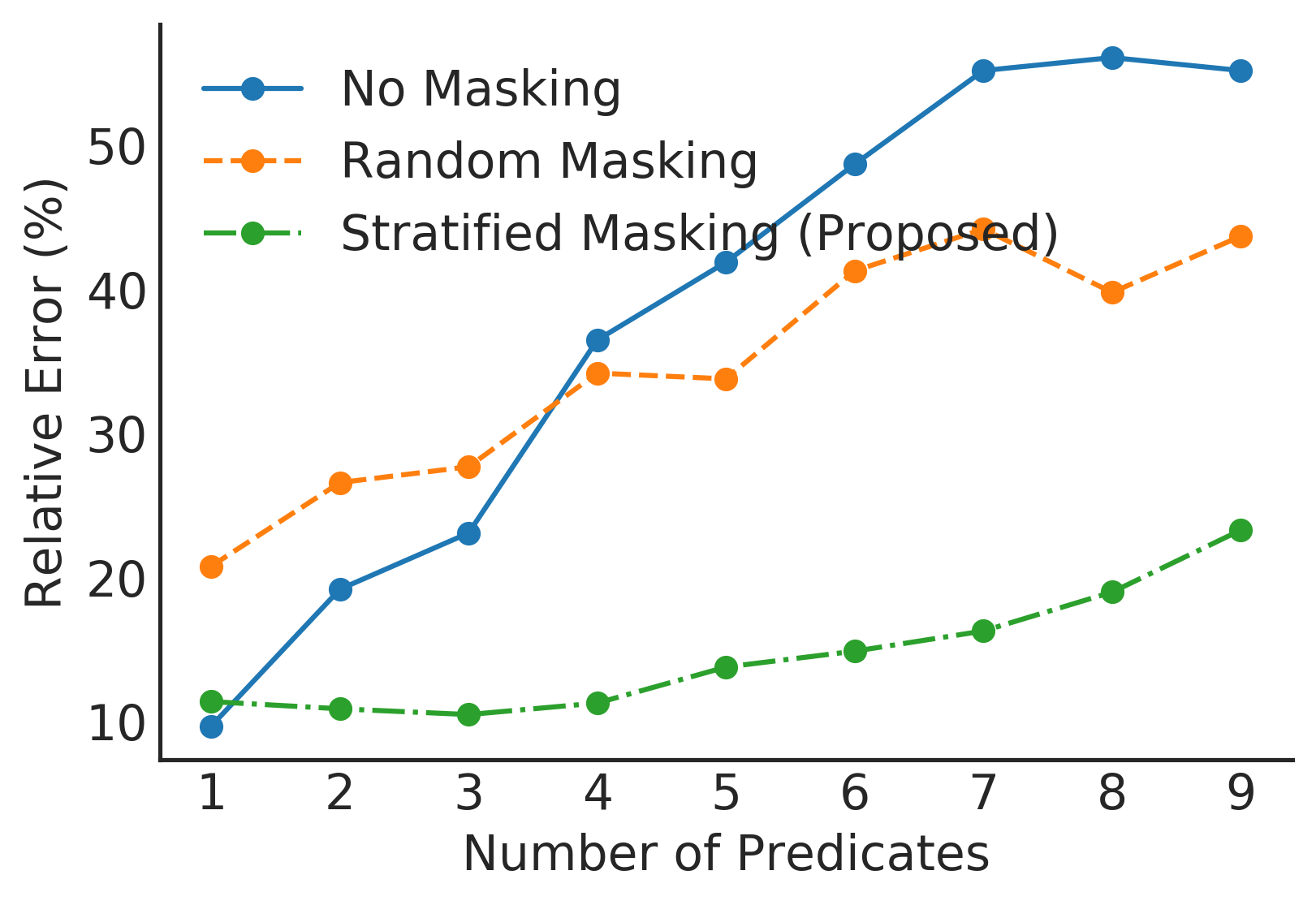
Figure 6: Masking strategy

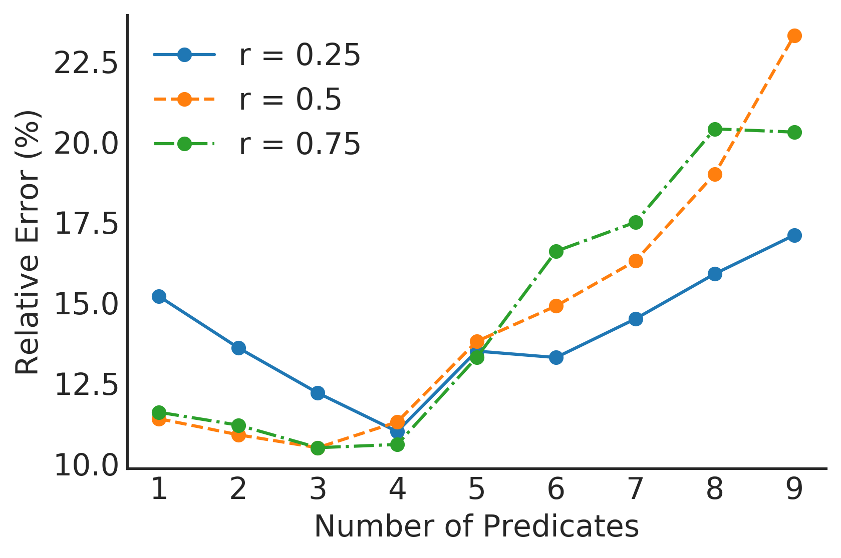
Figure 7: Masking factor

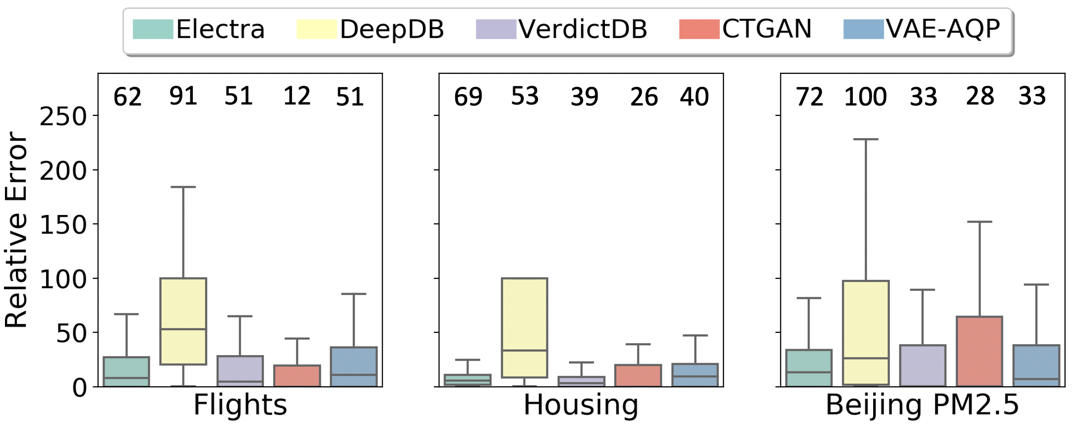
Figure 8: Error & bin-Completeness for GROUP BY queries

Performance on Production Workload

Fig. 5 shows the comparisons of the AQP error (as sMAPE) distribution for our production query workload for the three real-world datasets shown separately for AVG and SUM as the aggregate functions. For AVG as the aggregate function (Fig. 4(d)), Electra provides the lowest approximation error for both Housing and Beijing-PM-2.5 dataset. For Flights dataset, even though the median error is comparable to DeepDB, VerdictDB and VAE-AQP, the tail error is larger. Please note: since these plots were calculated over the production queries, 70% of the queries had two or fewer predicates. Thus, the benefit of Electra in handling large number of predicates is less visible. The percentages of queries that different techniques were able to successfully answer, are shown over the box-plots.

Performance on GROUP BY Queries

We evaluate Electra’s performance on GROUP BY queries using slight modification to our synthetic query workload by randomly choosing one of the attributes to be used for GROUP BY. We do not use any predicate on that attribute. Fig. 8 shows the AQP error over queries with all the different number of predicates. The error for each query was calculated as an average over the individual errors corresponding to each of the individual groups that were both present in the ground truth results and the approximate results. The error is computed as the average of the R.E. for each of the different groups corresponding to the GROUP BY column. Approximations might result in missing groups. We use bin-completeness measure as follows:

$$\textit{bin-completeness}=\frac{|G_{groups}\bigcap A_{groups}|}{|G_{groups}|}$$

$G_{groups}$ is the set of all the groups that appear in the ground truth and $A_{groups}$ is the set for the approximate result. This bin-completeness (§ 5) is an important measure for GROUP BY queries. Fig. 8 shows the bin-completeness numbers on top of the box plots. Higher is better. Both Electra and DeepDB can consistently provide much higher bin-completeness, compared to other baselines. However, the error for Electra is much better than DeepDB.

Design Components Analysis

Samples Generated per Query. Generating more representative samples by Electra can potentially improve accuracy, but at the cost of larger query latency and memory footprint. Table 1 shows the change in the R.E. for Electra as we increase the number of generated samples. Generating 1000 representative samples, from the learned conditional distribution, is good enough to achieve a low AQP error, and beyond that the improvement is not significant.

Impact of the Masking Strategy. Fig. 8 quantify the benefit of our proposed masking strategy for Flights dataset. We compare the proposed method with a No Masking strategy where only NaN input values, if any, are masked. We also compare with Random Masking strategy that uses a uniform random masking, irrespective of the column type (Ivanov, Figurnov, and Vetrov 2019). We observe that the proposed stratified masking strategy can significantly reduce the AQP error compared to the other two alternative, irrespective of the number of predicates used in the queries.

Masking factor. Fig. 8 shows the sensitivity of Electra corresponding to the masking factor, across the range of predicates for the Flights dataset. A masking factor of 0.5 would be the choice, if we want to optimize for queries with arbitrary number of predicates.

We provide more results, latency and memory profiling numbers for Electra along with discussion on future work in the supplement.

6 Related Work

Approximate Query Processing has a rich history with the use of sampling and sketching based approaches  (Chaudhuri, Ding, and Kandula 2017; Cormode 2011; Chaudhuri, Das, and Narasayya 2007). BlinkDB (Agarwal et al. 2013) uses offline sampling, but assumes it has access to historical queries to reduce or optimize for storage overhead. Related works used as baselines were described in § 5.

Representative Data Generation. With the advancement of deep-learning, multiple generative methods have been proposed, primarily using GAN(s) (Brock, Donahue, and Simonyan 2019) and VAE(s) (Ivanov, Figurnov, and Vetrov 2019). These techniques have been successful in producing realistic synthetic samples for images, auto-completing prompts for texts (Radford et al. 2019; Devlin et al. 2018), generating audio wavelets (Oord et al. 2016). Few works used GAN(s) (Xu et al. 2019; Park et al. 2018a) for tabular data generation either for providing data-privacy or to overcome imbalanced data problem.

Selectivity or Cardinality Estimation includes several classical methods with synopsis structures (e.g., histograms, sketches and wavelets) to provide approximate answers (Cormode et al. 2012). Recently, learned cardinality estimation methods have become common including using Deep Autoregressive models to learn density estimates of a joint data distribution  (Yang et al. 2019; Hasan et al. 2020; Yang et al. 2020), embedding and representation learning based cost and cardinality estimation  (Sun and Li 2019).

7 Conclusion

We presented a deep neural network based approximate query processing (AQP) system that can answer queries using a predicate-aware generative model at client-side, without processing the original data. Our technique learns the conditional distribution of data and generates targeted samples based on the conditions specified in the query. The key contributions of the paper are the use of conditional generative models for AQP and the techniques to reduce approximation error for queries with large number of predicates.

Appendix A Query Handling

Electra, like other recently proposed ML-based AQP techniques (Ma and Triantafillou 2019; Hilprecht et al. 2020; Thirumuruganathan et al. 2020) targets the most dominant query templates for exploratory data analytics. In Section “Target Query Structure”, we provided high-level characteristic of queries that Electra supports. Now we provide details about how exactly are these different classes of queries handled.

Conjunction predicates on categorical and discrete attributes: E.g. SELECT $\Psi$, AGG($A_{N_{i}}$) FROM $T$ WHERE $A_{C_{i}}=p$ AND $A_{C_{j}}=q$

A compound predicate composed of conjunctions (ANDs) in WHERE clauses is handled by using the specified predicate conditions on the discrete or categorical attributes as input to Electra’s conditional sample generator (masking other attributes) and then the query is executed on the generated samples to calculate the final answer.

Disjunction predicates on categorical and discrete attributes: E.g. SELECT $\Psi$, AGG($A_{N_{i}}$) FROM $T$ WHERE $A_{C_{i}}=p$ OR $A_{C_{i}}=q$

We support disjunctions (ORs) in WHERE conditions by decomposing it to multiple individual queries with each component of OR. We compute the AVG and COUNT of each individual query, and then use the COUNT as the weights to compute the overall AVG. For SUM, we directly compute the SUM of the individual queries.

If the OR conditions are on different variables, we use the principle of inclusion and exclusion to compute the required aggregate. For example, to compute $\pi$ = $(A_{C_{i}}=p$ OR $A_{C_{j}}=q)$, we will need to evaluate the queries, (1) $A_{C_{i}}=p$, (2) $A_{C_{j}}=q$ and (3) $(A_{C_{i}}=p$ AND $A_{C_{j}}=q)$, and then combine the results from these to obtain the result for the original query.

Note, Electra can handle any combinations of AND and OR conditions by converting it to Disjunctive Normal Form (i.e. converting it to a structure of [[.. AND ..] OR [.. AND ..]]) using Propositional Logic.

An IN (or ANY) condition can be similarly broken-down into multiple different predicates combined with OR and handled in the same manner.

Range predicates on continuous attributes: E.g. SELECT $\Psi$, AGG($A_{N_{i}}$) FROM $T$ WHERE $A_{N_{j}}$ BETWEEN $p$ AND $q$ . Electra is designed primarily for conditions on discrete or categorical attributes, which is the dominant usecase for exploratory data analytics. However, Electra can handle range queries on continuous attributes by converting it into discrete categories through discretization (or binning) for training. During sample generation, the range condition is converted into multiple OR-ed conditions, one for each discrete categories, and samples are generated and merged as discussed before. In the extreme case, Electra falls back to condition-less generation or only use the partial conditions (i.e. using only the discrete or categorical predicates) to first generate a broader range of samples and then apply the range predicates, specified on the continuous attributes, on those samples to further filter the samples before calculating the aggregate value.

Supporting GROUP BY: E.g. SELECT $\Psi$, AGG($A_{N_{i}}$) FROM $T$ WHERE $A_{C_{i}}=p$ GROUP BY $A_{C_{j}}$

Electra supports GROUP BY queries by decomposing it to multiple queries, one for each category of the categorical attribute on which the GROUP BY is done.

Different aggregates — AVG, SUM and COUNT: Electra answers the queries with AVG as the aggregate function by directly computing average on the samples generated in a predicate-aware manner from its generative model. Similarly, using the conditional selectivity estimation model, it can directly answer COUNT queries using the predicate as the input. To answer SUM queries, Electra first computes the average on the generated samples and then multiplies that with the selectivity estimate.

Supporting JOINs: Electra can support JOINs for predictable/popular joined datasets by first precomputing the JOIN-ed result table, then building the generative and selectivity estimation models on this resulting table. This approach is similar to other ML-based AQP techniques (Ma and Triantafillou 2019; Thirumuruganathan et al. 2020).

ORDER BY and LIMIT: Attributes that are used in ORDER BY can only be ones on which GROUP BY was applied or the attribute on which the aggregate was applied. Hence Electra can handle these queries without treating them specially. Low approximation error helps it mimic the ordering (and the set of records for LIMIT) as the fully accurate result.

Appendix B Implementation Details

In this section, we provide more details about the workload, datasets and the training methodology.

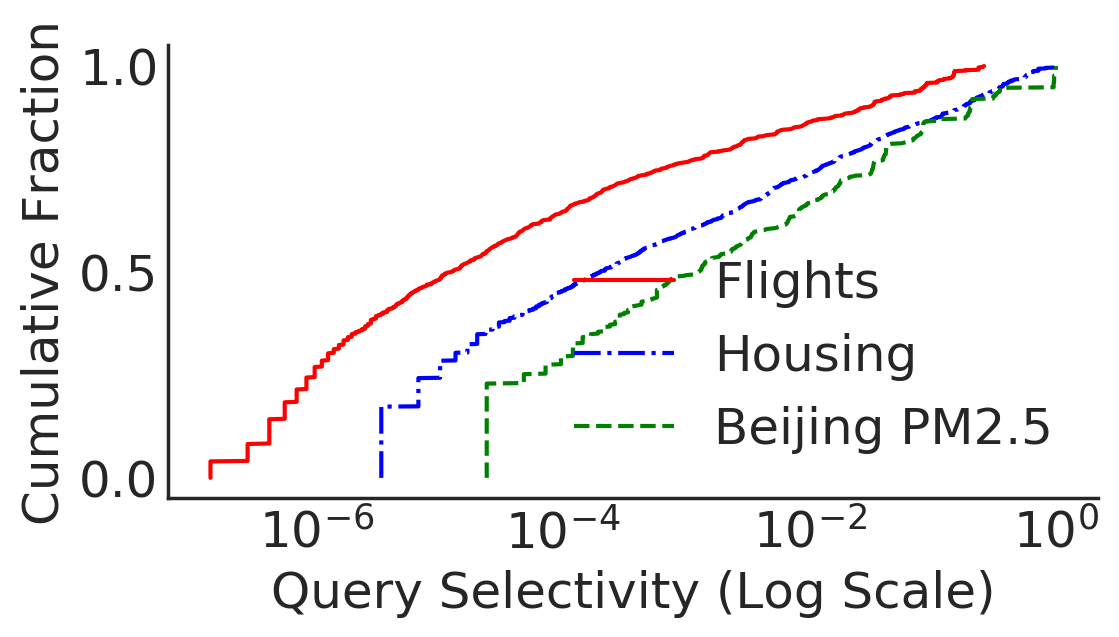
(a) Synthetic queries

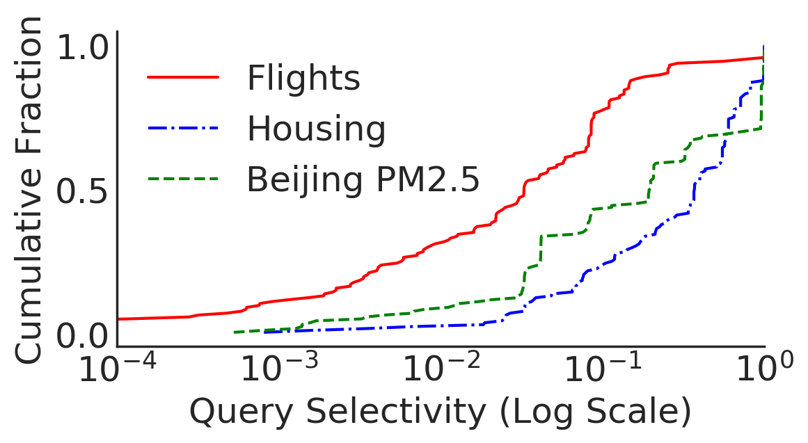
(b) Production queries

Figure 9: Workload selectivity characteristics

Dataset	# of Rows	# of Categorical	# of Numerical
Flights	7.26M	9	6
Housing	299K	14	4
Beijing PM2.5	43.8K	7	5

Table 2: Details of Real-World Datasets

Workload Characteristics

As described in the Section “Experimental Environment”, the synthetic query workload had the following SQL query template: SELECT AVG($n_{i}$) FROM T WHERE c1 = v1 AND … AND ck = vk Here $n_{i}$ is a numerical column, c1,…,ck are categorical columns and v1,…,vk are values taken by these categorical columns.

Fig. 9 shows how both the synthetic workload and production workload cover a wide range of query selectivity on the three real-world datasets.

Dataset Characteristics

The datasets described in the Section “Experimental Evaluation” had a mix of both categorical and numerical columns, ensuring that we train and evaluate Electra on diverse attribute sets making sure we learn to predict the values (of numerical attributes) while conditioning on predicates (categorical attributes). Table 2 describes the dataset statistics.

Training Methodology

Before training, we perform a set of pre-processing transformations on the dataset. We label encode the categorical attributes to convert the distinct categories to integer labels which are then used to create the one-hot vector. The unique values associated with a categorical attribute are stored and used for two purposes - first, during inference to transform the input query predicates to their encoded labels for input to the model and second, to identify the different groups while answering a GROUP BY query on these categorical attributes. For the numerical attributes, with multi-modal distribution we perform mode specific normalization. We use Kernel Density Estimation (KDE) with Scott’s (Scott 2015) bandwidth parameter selection to identify inflection points in the density estimates and then fit a Gaussian mixture. Numerical values are standard normalized using these obtained modes.

Appendix C Additional Experiments

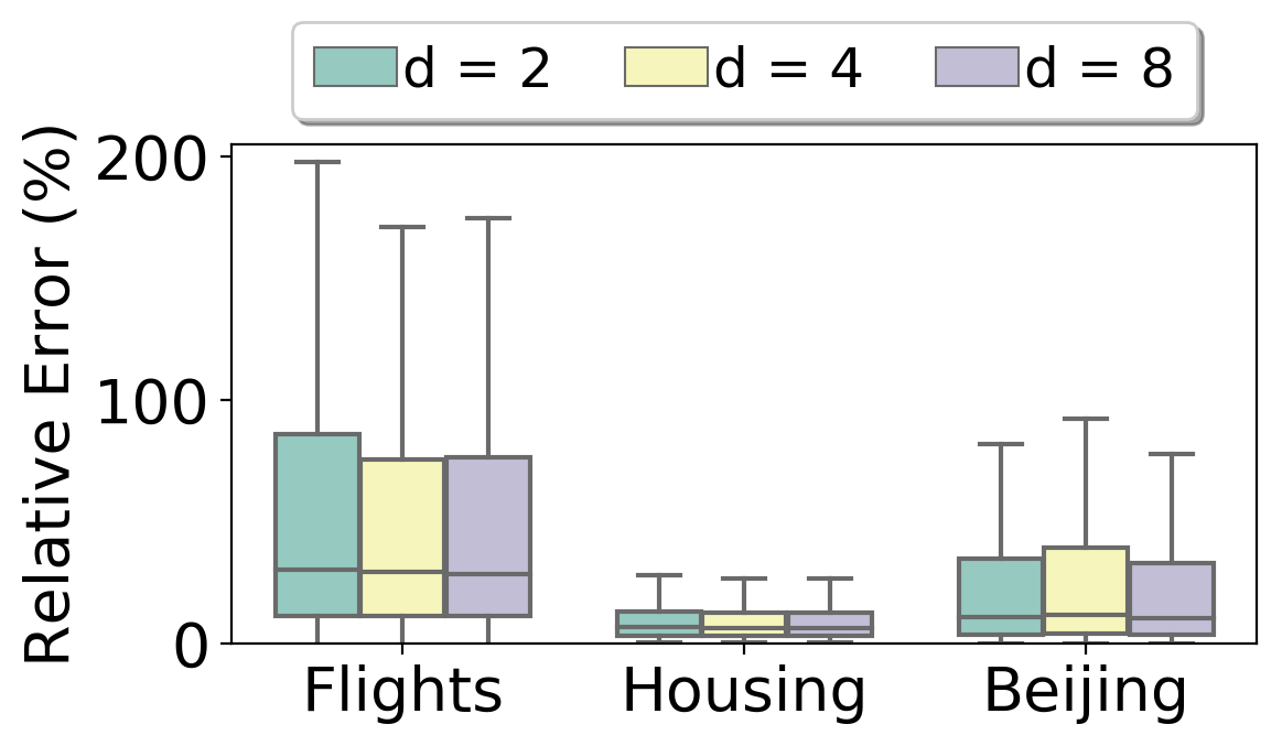
Figure 10: Network Depths

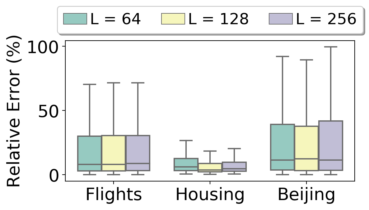
Figure 11: Latent Dimensions

Depth of Prior & Proposal Networks

In Fig. 11 we show the variations of AQP error, accumulated over all the queries with different number of predicates and for all three datasets. We set the depth ($d$) of both prior and proposal networks as 2, 4 and 8. While more depth and hence more complex network helps to achieve better accuracy, it can be observed it has a diminishing returns. More depth also increases the size of the model and requires longer time for the training to converge.

Latent Dimension

Latent dimension ($L$) was varied in Fig. 11 between 64, 128 and 256. While in theory a larger latent dimension would help to capture the conditional distribution at a finer resolution, we observed that 128 is the optimum value across all datasets.

Model Scalability

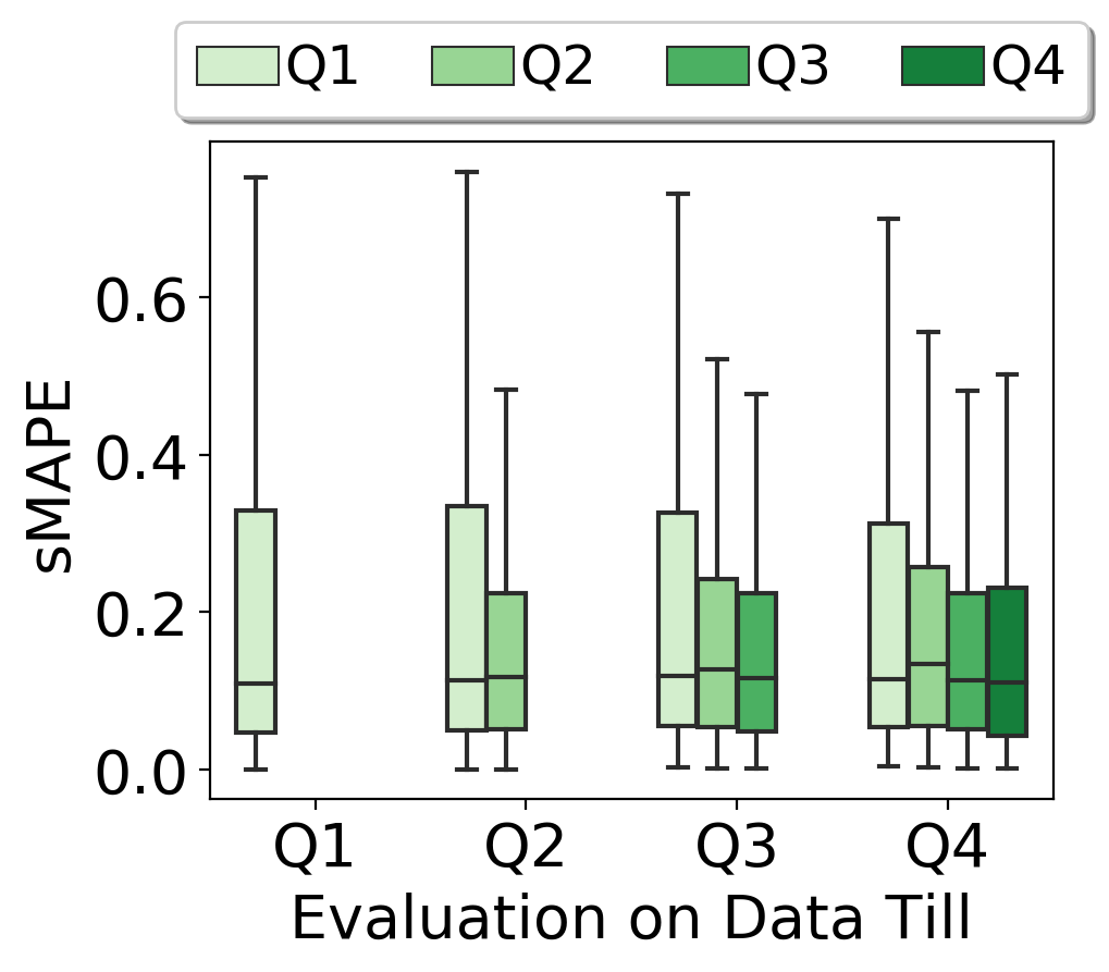
Figure 12: Performance of Electra with increase of data with new quarterly data ingestion for Flights dataset. We show how model trained on Q1 performs on data for Q1+Q2, Q1+Q2+Q3 and Q1+Q2+Q3+Q4, how model trained on Q1+Q2 performs on Q1+Q2+Q3 and Q1+Q2+Q3+Q4 and so on. Same model-size can keep the median error low with retraining, even when data size increases by 4 times.

Data	# Rows	mins/epoch	Model size
Q1	1.7M	3.19	15.08 MB
Q1-Q2	3.5M	6.18	15.08 MB
Q1-Q3	5.4M	8.56	15.08 MB
Q1-Q4	7.2M	11.41	15.08 MB

Table 3: Changes of data-size, re-training time and model-size.

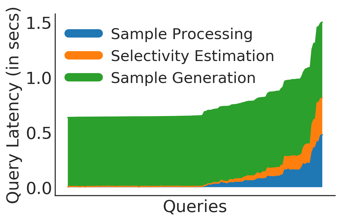
(a) Flights

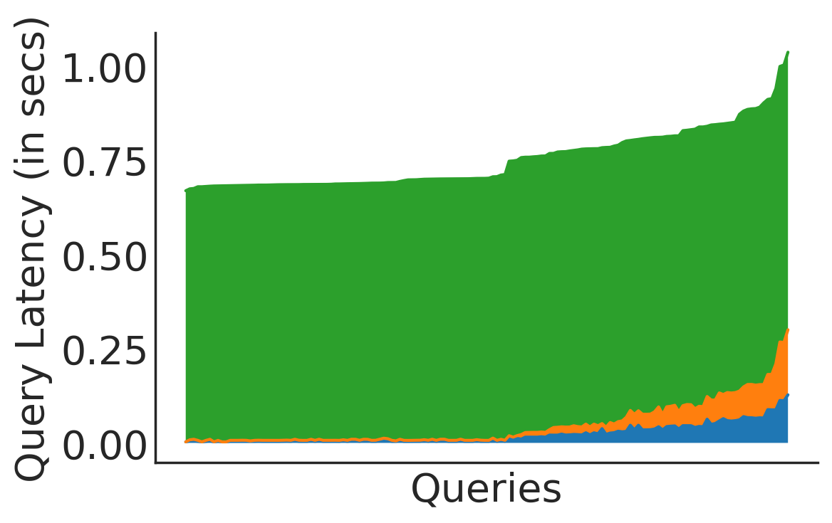
(b) Housing

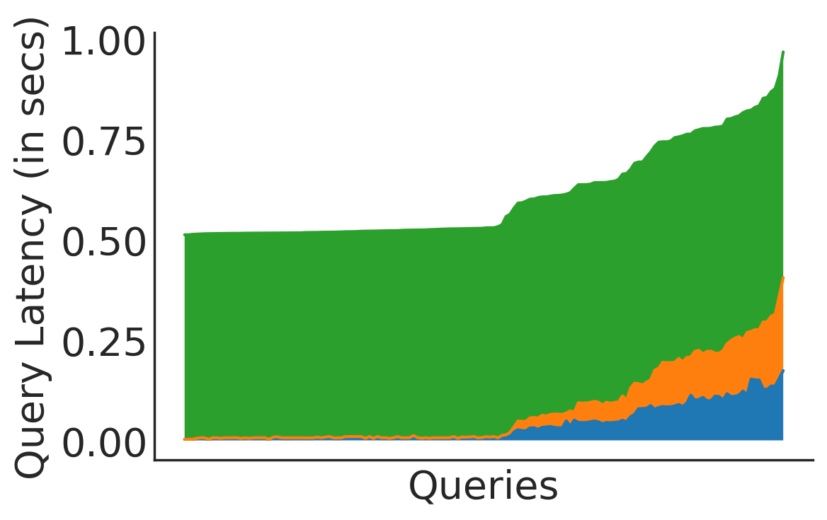
(c) Beijing PM 2.5

Figure 13: Query latency on production workload

In many real-world scenario, newly available data is periodically ingested to the system in batch and appended to the existing data on which analysts run queries to explore and find insights. In this section, we evaluate how the AQP error for Electra changes if we use the existing models to answer the queries that are targeted towards the whole of the newly appended data.

We do this using the Flights dataset and divide it into four quarters Q1-Q4 of 2019, using the already available Quarter column. Then we train Electra only with data till $Q_{i}$ where $i\in[1,4]$ and then evaluate using ground truth till $Q_{j}$ where $j\in[i,4]$. As shown in Fig. 12, we found Electra’s old models were able to keep the median AQP error low (with only some increase in the outliers), but the tail of the error-distributions increased when evaluated on the new data that is being progressively appended. Please note, in Fig. 12, the $Q_{i}$, $Q_{i}$ bars show that how much the AQP errors would reduce if Electra performs a retraining on the newly appended data. We can also see from the median latency plots, that retraining need not be performed for every data ingestion as the previously trained model can sustain low approximation error up to a mark and gradually increasing for additional fresh data ingestion. Needless to say, this observation is very much dependent on the characteristics of the actual data sources and Electra’s design has a module to specifically detect such shifts in the data distribution as part of its ETL logic for (re-)training.

In Table 3, we also show the variation in training time per epoch for different dataset sizes due to data ingestion. The models were trained for 50 epochs within which the VLB loss had converged. A similar convergence behavior was observed on other datasets. Note that the same model-size (15.08 MB) can bring down the error after retraining on data upto 4x large, while the training time per epoch linearly increases with the training data size. The model-size did not increase because hyperparameters of the architecture as well as the number of categories in the dataset did not change. In order to tame this for larger datasets, one can train on a sample of the original data depending on the time and resource availability.

Scalability of Electra model training phase can also be improved using parallel or distributed learning supported by all major deep-learning frameworks like Tensorflow and PyTorch. Other general distributed learning algorithms e.g., DownpourSGD, ADMM, EASGD, and GoSGD  can also be used to extend our approach for handling very large datasets. Electra can be trained even on a sampled data without much loss of accuracy. Finally, in case there are any attributes that are very frequently used, then original data can also be divided based on different categories of that attribute and multiple models, one corresponding to each part can be trained in parallel.

Query Latency and Memory Footprint

In this section we characterize Electra’s query processing latency, how different submodules contribute to that latency, along with its runtime memory footprint.

Latency: Figure 13(a),  13(b), 13(c) shows the end-to-end query latency for the production workload queries (sorted according to latency), also the time taken by different parts. Recall, Electra’s runtime workflow has 3 components: sample generation, sample processing and selectivity estimation. Sample processing involves calculating an average by executing the query on the initial 1000 samples generated. As discussed in § A, Electra decomposes a query into multiple subqueries for GROUP BYs and for OR, IN operators in WHERE conditions. Selectivity estimation is needed for both handling SUM as the aggregate, as well as for combining the results from multiple subqueries with appropriate weights. The queries towards the end are queries with large number of sub-queries increase, leading to higher latency. Particularly, true for Flights data where GROUP BY queries resulted in a larger number of subqueries due to columns with 50+ or even 360+ unique categories.

Dataset	Selectivity Estm.	Sample Gen.	Sample Processing
Flights	21.2	16.25	6.9
Housing	11.23	10.25	4.85
Beijing PM2.5	10.78	10.48	4.43

Table 4: Runtime Memory Usage (All numbers in MB).

Reducing Query Latency. Electra’s model size as well as inference latency can further be improved using post-training quantization techniques (Post-training Quantization ) available from deep-learning frameworks. We found that converting Electra’s model to ONNX format (ONNX ) (for running with Javascript, within a web-browser) can also significantly reduce its inference latency. Multiple sub-queries corresponding to disjunctions or GROUP BYs can potentially also be handled in parallel by different cores at the client-side to further reduce latency. A caching layer can be introduced at the client-side, to cache samples generated for frequently used combination of predicates latency improvements.

Memory Consumption. Peak runtime memory consumption was measured during the 3 stages of operation for Electra. using @profile decorator from python memory profiler (Memory Profiler ) module. From Table 4 it can be observed that peak memory was about 21.2 MB for Flights, 11.2 MB for Housing and 10.8 MB for Beijing PM 2.5. Across all datasets and memory peaks during selectivity estimation (S. E.) using Naru. Memory usage of Flights is higher because of some categories had large number of unique values that required higher one hot encoding dimension by Electra. Please note, that Electra can keep low runtime memory footprint, as it only generates a small number of sample on the fly to answer the queries and does not keep a large number of samples in memory.

Discussion: Please note, achieving the lowest latency is not our goal, rather lowering the approximation error for complex but critical queries is our goal, as long as the latency is still within the bounds of humans-speed for good user-experience. After talking to several experienced analysts, we understand $<1$ second latency, which we achieve for most of the queries (Fig. 13), is well within the bounds of human-speed for insight discovery use-cases. Having said that, we see significant scopes for improving latency by converting to special model formats (e.g. ONNX (ONNX.js )), using quantization (Post-training Quantization ) and parallelism across cores — including parallel inference between our CVAE and Naru models. None of these we have used in this paper. Quantization, pruning and other neural network compression techniques (Han, Mao, and Dally 2015) can also significantly reduce the model-size and hence the run-rime memory footprint. We leave it as a future work to characterize the approximation errors, latency and memory footprint for all ML-based AQP techniques, including Electra, when neural-network compression techniques and other forms of regularization are applied.

Appendix D Discussion and Future Work

We now discuss limitations of Electra and our future works.

Confidence Intervals (CI): We plan to focus on developing a CI calculation method for Electra. While providing an accurate CI is challenging for all AQP systems (Chaudhuri, Ding, and Kandula 2017). Some AQP systems (Agarwal et al. 2013; Hilprecht et al. 2020) provide a CI assuming a normal distribution for the predicted results. Electra might use a similar approach. But, we also plan to explore how bootstrapping (DiCiccio and Efron 1996) can be used to repeatedly sample the latent-space of our CVAE model to calculate a CI, which has never been done for a DNN-based generative model.

Additional Aggregates: Electra now supports AVG, SUM, COUNT aggregates over numerical columns. In the future, we plan to extend our technique to support to more type of aggregates such as MAX, MIN and COUNT DISTINCT. For COUNT DISTINCT, some promising approximation techniques are available using a combination of CountMin and HyperLogLog sketches (Ting 2019). We will investigate, how such techniques can be used at the client-side and integrated with Electra alongside or replacing Naru for cardinality estimation. Capturing MAX and MIN in a conditional generative model is a non-trivial problem. We will explore how to incorporate the concepts of extreme quantile estimation (Beirlant, Wet, and Goegebeur 2004) in the training process of our conditional generative model.

Incremental Retraining: As observed in Table 3, the retraining time of Electra scales linearly with size of data after fresh ingestion data batches. We observed that for very large datasets, Electra trained only on a small fraction of uniform samples (5-10%) can still answer queries with comparable relative error as the original data. If hints about important attributes in the queries are known a priori, such training can also be performed using a stratified sample. Such training over samples can significantly reduce the retraining-time when data-size keeps on growing. However, we plan to investigate how Electra’s model can be incrementally trained on the new data without catastrophic forgetting (Lee et al. 2017). Transfer learning (Zhuang et al. 2020) for generative or conditional generative models is also an untapped area, worth pursuing in this context.

No universal winner — Hybrid AQP System: Electra’s system design, as described in Section “Design of Electra ” allows the use of a server-side exact query processing mechanism for the query structures that Electra currently does not support (Ref. § A). However, a more intelligent design of a client-side hybrid AQP system should be investigated as well. The reason being, as observed from Figure 4 (AQP Error vs # of predicates), in the spectrum of queries with 1 to 9 (or more predicates), there is no universal winner. While DeepDB is the best-performing client-side technique for queries with 1-2 predicates, Electra is the best-performing technique for queries with more than 3 predicates. Similar to recently proposed mobile computer vision systems that keep multiple object classifiers or detectors to optimize for accuracy and latency for different video frames (Han et al. 2016), we can also explore how a hybrid ML-based AQP system can use different AQP models, depending on the query properties to optimize for accuracy and latency.

References

- Agarwal et al. (2013) Agarwal, S.; Mozafari, B.; Panda, A.; Milner, H.; Madden, S.; and Stoica, I. 2013. BlinkDB: Queries with Bounded Errors and Bounded Response Times on Very Large Data. In EuroSys.
- Beirlant, Wet, and Goegebeur (2004) Beirlant, J.; Wet, T. D.; and Goegebeur, Y. 2004. Nonparametric estimation of extreme conditional quantiles. Journal of statistical computation and simulation, 74(8): 567–580.
- Brock, Donahue, and Simonyan (2019) Brock, A.; Donahue, J.; and Simonyan, K. 2019. Large Scale GAN Training for High Fidelity Natural Image Synthesis. ArXiv, abs/1809.11096.
- Chaudhuri, Das, and Narasayya (2007) Chaudhuri, S.; Das, G.; and Narasayya, V. 2007. Optimized stratified sampling for approximate query processing. ACM Transactions on Database Systems.
- Chaudhuri, Ding, and Kandula (2017) Chaudhuri, S.; Ding, B.; and Kandula, S. 2017. Approximate Query Processing: No Silver Bullet. In SIGMOD.
- Chen (2017) Chen, S. X. 2017. UCI Machine Learning Repository.
- Cormode (2011) Cormode, G. 2011. Sketch techniques for approximate query processing. Foundations and Trends in Databases.
- Cormode et al. (2012) Cormode, G.; Garofalakis, M.; Haas, P. J.; and Jermaine, C. 2012. Synopses for Massive Data: Samples, Histograms, Wavelets, Sketches. Foundation and Trends in Databases.
- Crotty et al. (2015) Crotty, A.; Galakatos, A.; Zgraggen, E.; Binnig, C.; and Kraska, T. 2015. Vizdom: Interactive Analytics through Pen and Touch. Proc. VLDB Endow.
- Crotty et al. (2016) Crotty, A.; Galakatos, A.; Zgraggen, E.; Binnig, C.; and Kraska, T. 2016. The Case for Interactive Data Exploration Accelerators (IDEAs). In HILDA.
- (11) CTGAN code. 2019. CTGAN Github Repo. https://github.com/sdv-dev/CTGAN.
- (12) DeepDB code. 2020. DeepDB Github Repo. https://github.com/DataManagementLab/deepdb-public.
- Devlin et al. (2018) Devlin, J.; Chang, M.-W.; Lee, K.; and Toutanova, K. 2018. Bert: Pre-training of deep bidirectional transformers for language understanding. arXiv preprint arXiv:1810.04805.
- DiCiccio and Efron (1996) DiCiccio, T. J.; and Efron, B. 1996. Bootstrap confidence intervals. Statistical science, 11(3): 189–228.
- Han, Mao, and Dally (2015) Han, S.; Mao, H.; and Dally, W. J. 2015. Deep compression: Compressing deep neural networks with pruning, trained quantization and huffman coding. arXiv preprint arXiv:1510.00149.
- Han et al. (2016) Han, S.; Shen, H.; Philipose, M.; Agarwal, S.; Wolman, A.; and Krishnamurthy, A. 2016. Mcdnn: An approximation-based execution framework for deep stream processing under resource constraints. In Proceedings of the 14th Annual International Conference on Mobile Systems, Applications, and Services.
- Hasan et al. (2020) Hasan, S.; Thirumuruganathan, S.; Augustine, J.; Koudas, N.; and Das, G. 2020. Deep Learning Models for Selectivity Estimation of Multi-Attribute Queries. In SIGMOD.
- Hilprecht et al. (2020) Hilprecht, B.; Schmidt, A.; Kulessa, M.; Molina, A.; Kersting, K.; and Binnig, C. 2020. DeepDB: Learn from Data, Not from Queries! Proc. VLDB Endow.
- Ivanov, Figurnov, and Vetrov (2019) Ivanov, O.; Figurnov, M.; and Vetrov, D. 2019. Variational Autoencoder with Arbitrary Conditioning. In ICLR.
- Kingma and Welling (2014) Kingma, D. P.; and Welling, M. 2014. Auto-Encoding Variational Bayes. In ICLR.
- Kraska et al. (2018) Kraska, T.; Beutel, A.; Chi, E. H.; Dean, J.; and Polyzotis, N. 2018. The case for learned index structures. In SIGMOD.
- Lee et al. (2017) Lee, S.-W.; Kim, J.-H.; Jun, J.; Ha, J.-W.; and Zhang, B.-T. 2017. Overcoming catastrophic forgetting by incremental moment matching. arXiv preprint arXiv:1703.08475.
- Liu and Heer (2014) Liu, Z.; and Heer, J. 2014. The Effects of Interactive Latency on Exploratory Visual Analysis. IEEE Transactions on Visualization and Computer Graphics.
- Ma and Triantafillou (2019) Ma, Q.; and Triantafillou, P. 2019. DBEst: Revisiting Approximate Query Processing Engines with Machine Learning Models. In SIGMOD.
- (25) Memory Profiler. 2020. Python Memory Profiler. https://pypi.org/project/memory-profiler/.
- Mirhoseini et al. (2017) Mirhoseini, A.; Pham, H.; Le, Q. V.; Steiner, B.; Larsen, R.; Zhou, Y.; Kumar, N.; Norouzi, M.; Bengio, S.; and Dean, J. 2017. Device placement optimization with reinforcement learning. In ICML.
- Mondal, Sheoran, and Mitra (2021) Mondal, S. S.; Sheoran, N.; and Mitra, S. 2021. Scheduling of Time-Varying Workloads Using Reinforcement Learning. In AAAI Conference on Artificial Intelligence.
- of Transportation Statistics (2019) of Transportation Statistics, B. 2019. Carrier On-Time Performance.
- (29) ONNX. 2017. Open Neural Network Exchange. https://github.com/onnx/onnx.
- (30) ONNX.js. 2018. ONNX.js. https://github.com/microsoft/onnxjs.
- Oord et al. (2016) Oord, A. v. d.; Dieleman, S.; Zen, H.; Simonyan, K.; Vinyals, O.; Graves, A.; Kalchbrenner, N.; Senior, A.; and Kavukcuoglu, K. 2016. Wavenet: A generative model for raw audio. arXiv preprint arXiv:1609.03499.
- Park et al. (2018a) Park, N.; Mohammadi, M.; Gorde, K.; Jajodia, S.; Park, H.; and Kim, Y. 2018a. Data Synthesis Based on Generative Adversarial Networks. Proc. VLDB.
- Park et al. (2018b) Park, Y.; Mozafari, B.; Sorenson, J.; and Wang, J. 2018b. VerdictDB: Universalizing Approximate Query Processing. In SIGMOD.
- (34) Post-training Quantization. 2019. Tensorflow Post-training Quantization. https://www.tensorflow.org/lite/performance/post˙training˙quantization.
- Qiu (2018) Qiu, Q. 2018. Housing Price in Beijing. https://www.kaggle.com/ruiqurm/lianjia/version/2.
- Radford et al. (2019) Radford, A.; Wu, J.; Child, R.; Luan, D.; Amodei, D.; Sutskever, I.; et al. 2019. Language models are unsupervised multitask learners. OpenAI blog, 1(8): 9.
- Scott (2015) Scott, D. W. 2015. Multivariate Density Estimation. Wiley Series in Probability and Statistics. John Wiley & Sons, Inc.
- Sohn, Lee, and Yan (2015) Sohn, K.; Lee, H.; and Yan, X. 2015. Learning Structured Output Representation using Deep Conditional Generative Models. In Advances in Neural Information Processing Systems.
- Stolte, Tang, and Hanrahan (2002) Stolte, C.; Tang, D.; and Hanrahan, P. 2002. Polaris: A system for query, analysis, and visualization of multidimensional relational databases. IEEE Transactions on Visualization and Computer Graphics.
- Sun and Li (2019) Sun, J.; and Li, G. 2019. An end-to-end learning-based cost estimator. arXiv preprint arXiv:1906.02560.
- Thirumuruganathan et al. (2020) Thirumuruganathan, S.; Hasan, S.; Koudas, N.; and Das, G. 2020. Approximate Query Processing for Data Exploration using Deep Generative Models. In 36th IEEE ICDE.
- Ting (2019) Ting, D. 2019. Approximate distinct counts for billions of datasets. In SIGMOD.
- (43) VerdictDB code. 2018. Verdict Project. https://github.com/verdict-project/verdict.
- Xu et al. (2019) Xu, L.; Skoularidou, M.; Cuesta-Infante, A.; and Veeramachaneni, K. 2019. Modeling Tabular data using Conditional GAN. In Advances in Neural Information Processing Systems.
- Yang et al. (2020) Yang, Z.; Kamsetty, A.; Luan, S.; Liang, E.; Duan, Y.; Chen, X.; and Stoica, I. 2020. NeuroCard: One Cardinality Estimator for All Tables. Proc. VLDB Endow.
- Yang et al. (2019) Yang, Z.; Liang, E.; Kamsetty, A.; Wu, C.; Duan, Y.; Chen, X.; Abbeel, P.; Hellerstein, J. M.; Krishnan, S.; and Stoica, I. 2019. Deep Unsupervised Cardinality Estimation. Proc. VLDB Endow.
- Zhuang et al. (2020) Zhuang, F.; Qi, Z.; Duan, K.; Xi, D.; Zhu, Y.; Zhu, H.; Xiong, H.; and He, Q. 2020. A comprehensive survey on transfer learning. Proceedings of the IEEE, 109(1): 43–76.