An asymptotic approach to Borwein-type sign pattern theorems

Abstract.

The celebrated (First) Borwein Conjecture predicts that for all positive integers $n$ the sign pattern of the coefficients of the “Borwein polynomial”

$$(1-q)(1-q^{2})(1-q^{4})(1-q^{5})\cdots(1-q^{3n-2})(1-q^{3n-1})$$

is $+--+--\cdots$. It was proved by the first author in [Adv. Math. 394 (2022), Paper No. 108028]. In the present paper, we extract the essentials from the former paper and enhance them to a conceptual approach for the proof of “Borwein-like” sign pattern statements. In particular, we provide a new proof of the original (First) Borwein Conjecture, a proof of the Second Borwein Conjecture (predicting that the sign pattern of the square of the “Borwein polynomial” is also $+--+--\cdots$), and a partial proof of a “cubic” Borwein Conjecture due to the first author (predicting the same sign pattern for the cube of the “Borwein polynomial”). Many further applications are discussed.

1. Introduction

It was in 1993 at a workshop at Cornell University, when what became known as the Borwein Conjecture was born. (One of the authors was an intrigued witness of this event.) George Andrews delivered a two-part lecture on “AXIOM and the Borwein Conjecture”, in which he — first of all — stated three conjectures that had been communicated to him by Peter Borwein (the first of which became known as “the Borwein Conjecture”), and then reported the lines of attack that he had tried, all of which had failed to give a proof, stressing (quoting from [1], which contains Andrews’ findings in printed form) that “this is the sort of intriguing simply stated problem that devotees of the theory of partitions love.” Indeed, the statement of the first conjecture, dubbed the “First Borwein Conjecture” in [1], is the following.

Conjecture 1.1 (P. Borwein).

For all positive integers $n$, the sign pattern of the coefficients in the expansion of the polynomial $P_{n}(q)$ defined by

$$P_{n}(q):=(1-q)(1-q^{2})(1-q^{4})(1-q^{5})\cdots(1-q^{3n-2})(1-q^{3n-1})$$ (1.1)

is $+--+--+--\cdots$, with a coefficient $0$ being considered as both $+$ and $-$.

The Second Borwein Conjecture from [1] predicts the same sign behaviour of the coefficients for the square of the “Borwein polynomial”.

Conjecture 1.2 (P. Borwein).

For all positive integers $n$, the sign pattern of the coefficients in the expansion of the polynomial $P_{n}^{2}(q)$, where $P_{n}(q)$ is defined by (1.1), is $+--+--+--\cdots$, with the same convention concerning zero coefficients.

The Third Borwein Conjecture from [1] is an assertion on the sign behaviour of the coefficients of a polynomial similar to $P_{n}(q)$, where however the involved modulus is $5$ instead of $3$. We shall return to it at the end of this paper, see Conjecture 11.1 in Section 11.

Interestingly, the first author observed recently that a cubic version of the conjecture also appears to hold, which both Borwein and Andrews missed.

Conjecture 1.3 (C. Wang).

For all positive integers $n$, the sign pattern of the coefficients in the expansion of the polynomial $P_{n}^{3}(q)$, where $P_{n}(q)$ is defined by (1.1), is $+--+--+--\cdots$, with the same convention concerning zero coefficients as before.

These deceivingly simple conjectures intrigued many researchers after Andrews had introduced them to a larger audience — in particular the first one, Conjecture 1.1. Various approaches were tried — combinatorial, or using $q$-series techniques (cf. e.g. [1, 4, 5, 8, 11, 14, 17, 18, 19]) —, variations and generalisations were proposed (see [6, 8, 11, 14]) — most notably Bressoud’s conjecture in [8] — sometimes leading to proofs of related results. However, none of these attempts came anything close to progress concerning the original First Borwein Conjecture, Conjecture 1.1. It took almost 30 years until the first author succeeded in proving this conjecture in [16], using analytic means.

Starting point of the proof in [16] was explicit sum representations of the polynomials $A_{n}(q),B_{n}(q),C_{n}(q)$ in the decomposition of $P_{n}(q)$ given by

$$P_{n}(q)=A_{n}(q^{3})-qB_{n}(q^{3})-q^{2}C_{n}(q^{3}),$$ (1.2)

due to Andrews [1]. It should be noted that the First Borwein Conjecture, Conjecture 1.1, is equivalent to the statement that all coefficients of the polynomials $A_{n}(q),B_{n}(q),C_{n}(q)$ are non-negative. These coefficients were written in [16] in terms of the obvious Cauchy integrals. Subsequent saddle point approximations showed that for $n>7000$ the coefficient of $q^{m}$ in $A_{n}(q),B_{n}(q),C_{n}(q)$ is positive in the range $n<m<n^{2}-n$. The proof could then be completed by appealing to another result of Andrews [1] which gives non-negativity of the coefficients of $q^{m}$ in $A_{n}(q),B_{n}(q),C_{n}(q)$ for $m\leq n$ and $m\geq n^{2}-n$ “for free”, and by performing a computer check of the conjecture for $n\leq 7000$.

At this point, it must be mentioned that formulae analogous to Andrews’ formulae for the decomposition polynomials $A_{n}(q),B_{n}(q),C_{n}(q)$ are not available for the analogous decompositions of $P_{n}^{2}(q)$ or $P_{n}^{3}(q)$, or for the corresponding decomposition of the polynomial $S_{n}(q)$ in the Third Borwein Conjecture (Conjecture 11.1), and that it is unlikely that such formulae exist.

Thus, the article [16] left open the question whether it was just an isolated instance that this approach succeeded to prove the First Borwein Conjecture, or whether similar ideas could also lead to proofs of the Second and Third Borwein Conjecture, or of the new Conjecture 1.3. Admittedly, since the proof in [16] relied on Andrews’ sum representations for the decomposition polynomials $A_{n}(q),B_{n}(q),C_{n}(q)$ in an essential way, at the time it did not seem very realistic to expect that, with these ideas, one could go beyond the First Borwein Conjecture.

In the meantime, however, we realised that, instead of relying on Andrews’ sum representations for the decomposition polynomials, the saddle point approximation idea could be directly applied to $P_{n}(q)$ and its powers, and, when doing this, surprisingly the quantities that have to be approximated are very similar to those that were at stake in [16] (compare, for instance, the sum over $m$ at the beginning of the proof of Proposition 11.1 in [16] with (9.1) below, or [16, Lemma B.3] and Lemma A.10). There is a price to pay though: while in [16] the (dominant) saddle points were located on the real axis, with this new approach we have to deal with (dominant) saddle points located at complex points. This makes the estimations that have to be performed more delicate. On the positive side, it allows one to proceed in a more streamlined fashion — for example, here we do not have to deal with several different kinds of peaks along the integration contour, as opposed to [16] where an unbounded number of peaks of two different kinds had to be considered; here we encounter only two peaks that are (complex) conjugate to each other. Most importantly, it allows us to provide a uniform proof of the First and Second Borwein Conjecture, as well as a partial proof of the cubic conjecture, and altogether this is not longer than the proof of “just” the First Borwein Conjecture in [16].

In the next section, we provide an outline of our proof of Conjectures 1.1 and 1.2, and of “two thirds” of Conjecture 1.3. Very roughly, the approach that we put forward consists of the following steps:

1. show that the conjectures hold for the “first few” and the “last few” coefficients (see Part A in Section 2);

2. represent the coefficients by a contour integral (see Part B in Section 2);

3. divide the contour into two parts, the “peak part” (the part close to the dominant saddle points of the integrand) and the remaining part, the “tail part” (see Part C in Section 2);

4. for “large” $n$ (where “large” is made precise), bound the error made by approximating the “peak part” by a Gaußian integral (the “peak error”) (see Part D in Section 2);

5. for “large” $n$, bound the error contributed by the “tail part” (the “tail error”) (see Part D in Section 2);

6. verify the conjectures for “small” $n$ (see Part E in Section 2);

7. put everything together to complete the proofs (see Part E in Section 2).

The details are then filled in in the subsequent sections. More precisely, in Section 3 we explain how prior results of Andrews, of Kane, and of Borwein, Borwein and Garvan confirm the conjectures for the “first few” and the “last few” coefficients. Section 4 prepares some notation and preliminary material on log-derivatives of the “Borwein polynomial” $P_{n}(q)$ that is used ubiquitously in the subsequent sections. In Section 5, we make our choice of contour for the integral representation precise: it is a circle whose radius satisfies an equation, namely (5.1), that approximates the actual saddle point equation. Lemma 5.1 presents fundamental properties that this choice satisfies. In Section 6, we make precise how we divide the contour into the “peak part” and the “tail part”. Lemma 6.1 in that section presents first properties of this cutoff, to be used in the later parts of the paper. The fundamental inequality that is derived from this subdivision of the integral contour is the subject of Section 7. Namely, Lemma 7.1 provides a qualitative upper bound for the resulting approximation of the coefficients of $P_{n}^{\delta}(q)$, with $\delta\in\{1,2,3\}$, in terms of a peak error term and a tail error term. How to bound the peak error efficiently from above is shown in Section 8. This section contains in particular a fundamental result on the approximation of a (complex) function by a Gaußian integral that may be of independent interest for other applications; see Lemma 8.1. Subsequently, Section 9 is devoted to bound the tail error from above. Finally, in Section 10 we put everything together and complete the proofs of Conjectures 1.1 and 1.2, and of “two thirds” of Conjecture 1.3.

Without any doubt, several of the arguments that we need are quite technical. In the interest of not losing pace (too much) while guiding the reader through our proofs, we have “outsourced” some of the auxiliary results and have collected them in an appendix.

It must be emphasised though that a certain “level of technicality” is unavoidable since the approximations that we are carrying out here go with an intrinsic subtlety (already present in [16]) that is absent in most applications of the saddle point approximation technique: our goal is to show that the coefficients of $q^{m}$ in the “Borwein polynomial” $P_{n}(q)$ (respectively in its powers) obey a certain sign pattern, with $m$ running through a range that includes the asymptotic orders $O(n^{\omega})$, where $1\leq\omega\leq 2$. Consequently, our estimations must hold for that entire range, which makes it necessary to manage expressions that contain the radius $r$ of our contour that is solution of the approximate saddle point equation (5.1) without further specification of its asymptotic order, as for example in the definition of the cutoff in (6.1). The “best” that we can say about $r$ is its range as given in Lemma 5.1 (which again — necessarily — covers several different asymptotic orders in terms of $n$ at logarithmic scale).

The last section, Section 11, is devoted to a discussion of our approach and further applications. We start by explaining what is missing for the completion of the proof of Conjecture 1.3. We discuss the applicability of our methods for proving the Third Borwein Conjecture (see Conjecture 11.1), a conjecture of Ismail, Kim and Stanton vastly generalising the First Borwein Conjecture (see Conjecture 11.2), or related or similar conjectures, including some new ones that we present in this last section (in particular Conjectures 11.3 and 11.5). We also point out that the Bressoud Conjecture might as well be amenable to the ideas developed in this paper. Finally, we contemplate on the question whether the Borwein Conjecture(s) should be considered as combinatorial or analytic, a question which is evidently raised by our proof(s) (and other observations).

2. An outline of the proof

Here, we provide a brief outline of our proof of Conjectures 1.1 and 1.2, and of a part of Conjecture 1.3. From here on, we use the standard notation for $q$-shifted factorials,

$$(\alpha;q)_{n} =(1-\alpha)(1-\alpha q)\cdots(1-\alpha q^{n-1}),\text{ for }n\geq 1,$$

$$(\alpha;q)_{0} =1.$$

If $|q|<1$, or in the sense of formal power series in $q$, this definition also makes sense for $n=\infty$. Using this notation, the “Borwein polynomial” can be written as

$$P_{n}(q)=\frac{(q;q)_{3n}}{(q^{3};q^{3})_{n}}.$$

Furthermore, in the following we shall write $[q^{m}]P(q)$ for the coefficient of $q^{m}$ in the polynomial $P(q)$.

Our goal is to show that the sign pattern of the coefficients

$$[q^{m}]P_{n}^{\delta}(q),\quad m=0,1,2,\dots,$$

is $+--+--+--\cdots$, where $\delta$ is $1$, $2$, or $3$.

Our proof is composed of several parts.

A. The conjectures hold for the “first” $3n+1$ coefficients and the “last” $3n+1$ coefficients. We observe that the first few coefficients of $P_{n}^{\delta}(q)$ and $P_{\infty}^{\delta}(q)$, with $\delta\in\{1,2,3\}$, are identical. More precisely, we have

$$[q^{m}]P_{n}^{\delta}(q)=[q^{m}]P_{\infty}^{\delta}(q)$$ (2.1)

for $0\leq m\leq 3n$ and $\delta\in\{1,2,3\}$ (actually for all integers $\delta$). By a result of Andrews [1] this implies the sign pattern of the first $3n+1$ coefficients of $P_{n}(q)$ as predicted by Conjecture 1.1. Similarly, by a result of Kane [12], this implies the sign pattern of the first $3n+1$ coefficients of $P_{n}^{2}(q)$ as predicted by Conjecture 1.2. By using a result of Borwein, Borwein and Garvan [7], this also implies the sign pattern of the first $3n+1$ coefficients of $P_{n}^{3}(q)$ as predicted by Conjecture 1.3. See Section 3 for the details.

Combining the above observation with the fact that $P_{n}(q)$, and hence $P_{n}^{\delta}(q)$ for all $\delta$, is palindromic, it remains to show that the coefficients of $q^{m}$ in $P_{n}^{\delta}(q)$ for $3n\leq m\leq(\delta\deg P_{n})/2$ follow the sign pattern predicted by Conjectures 1.1–1.3.

B. Contour integral representation of the coefficients of $P_{n}^{\delta}(q)$. From now on, for convenience, we shall often use $Q_{n}(q)$ to denote $P_{n}^{\delta}(q)$, where $\delta$ is $1$, $2$, or $3$.

Using Cauchy’s integral formula, the coefficient $[q^{m}]Q_{n}(q)$ can be represented as the integral

$$\frac{1}{2\pi i}\int_{\Gamma}Q_{n}(q)\frac{dq}{q^{m+1}},$$

where $\Gamma$ is any contour about $0$ with winding number 1. We will choose $\Gamma$ as a circle centred at $0$ with radius $r$ for some $r\in\mathbb{R}^{+}$, so that the integral becomes

$$[q^{m}]Q_{n}(q)=\frac{r^{-m}}{2\pi}\int_{-\pi}^{\pi}Q_{n}\left(re^{i\theta}\right)e^{-im\theta}\,d\theta.$$ (2.2)

C. The saddle point approximation. The exact choice of $r$ is related to the saddle points of $q\mapsto|q^{-m}Q_{n}(q)|$, and we will elaborate on this in Section 5. The appropriate choice for $r$ is a value smaller than $1$ but close to $1$, see Lemma 5.1.

Figure 1 illustrates the typical behaviour of $\theta\mapsto|P_{n}\left(re^{i\theta}\right)|$ on the circle $\{z\in\mathbb{C}:|z|=r\}$. In particular, we can observe the following general features in the graph:

• the function has two peaks close to $\theta=2\pi/3$ and $\theta=-2\pi/3$;

• the function values outside small neighbourhoods of $\theta=2\pi/3$ and $\theta=-2\pi/3$ are very small compared to the peak value.

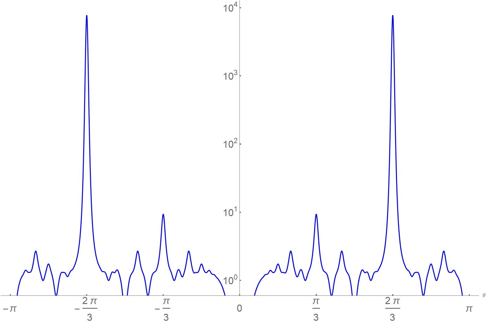
Figure 1. Modulus of $P_{81}(0.95e^{i\theta})$. The vertical axis has logarithmic scale.

Based on these heuristics, we choose a cutoff $\theta_{0}$ (to be determined in (6.1) in Section 6), and distinguish the following parts of the interval $[-\pi,\pi]$:

• The peak part $I_{\text{peak}}:=[-2\pi/3-\theta_{0},-2\pi/3+\theta_{0}]\cup[2\pi/3-\theta_{0},2\pi/3+\theta_{0}]$.

• The tail part $I_{\text{tail}}:=[-\pi,\pi]\setminus I_{\text{peak}}$.

Naturally, the integral (2.2) can be divided into two subintegrals corresponding to the two parts above.

We make the following observations concerning the subintegrals:

$\bullet$ The subintegral $\int_{I_{\text{peak}}}Q_{n}\left(re^{i\theta}\right)e^{-im\theta}\,d\theta$ can be approximated by a Gaußian integral. More specifically, if we define

$$g_{Q_{n}}(r)=\left.-\operatorname{Re}\frac{\partial^{2}}{\partial\theta^{2}}\log Q_{n}(re^{i\theta})\right|_{\theta=2\pi/3},$$ (2.3)

then we have

$$\int^{2\pi/3+\theta_{0}}_{2\pi/3-\theta_{0}}Q_{n}(re^{i\theta})e^{-im\theta}\,d\theta =e^{-2\pi mi/3}\int_{-\theta_{0}}^{\theta_{0}}Q_{n}(re^{i(\theta+2\pi/3)})e^{-im\theta}\,d\theta$$

$$\approx e^{-2\pi mi/3}Q_{n}(re^{2\pi i/3})\int_{-\theta_{0}}^{\theta_{0}}e^{-g_{Q_{n}}(r)\theta^{2}/2}\,d\theta$$

$$=e^{-2\pi mi/3}Q_{n}(re^{2\pi i/3})\frac{\sqrt{2\pi}}{\sqrt{g_{Q_{n}}(r)}}\operatorname{erf}\left(\frac{\theta_{0}\sqrt{g_{Q_{n}}(r)}}{\sqrt{2}}\right).$$ (2.4)

Here, “$\approx$” means “approximated by”. Since $Q_{n}(q)$ is a polynomial with real coefficients, we have $Q_{n}(\bar{z})=\overline{Q_{n}(z)}$. Therefore, an analogous approximation holds for the other interval of $I_{\text{peak}}$, that is, for the integral over $\theta$ in $[-2\pi/3-\theta_{0},-2\pi/3+\theta_{0}]$. The error made by these approximations is captured by the term $\epsilon_{0,Q_{n}}(m,r)$ defined below.

$\bullet$ The subintegral over $I_{\text{tail}}$ can be bounded above by

$$\left|\int_{I_{\text{tail}}}Q_{n}(re^{i\theta})e^{-im\theta}\,d\theta\right|\leq\left|Q_{n}(re^{2\pi i/3})\right|\int_{I_{\text{tail}}}\left|\frac{Q_{n}(re^{i\theta})}{Q_{n}(re^{2\pi i/3})}\right|\,d\theta.$$ (2.5)

The error of this approximation is captured by the term $\epsilon_{1,Q_{n}}(r)$ defined below.

D. Bounding the errors. Our next step is to estimate the error in the approximation (2.4) of the peak part, and to bound the tail part (2.5) of the integral. Accordingly, we define the error terms $\epsilon_{0,Q_{n}}(m,r)$ and $\epsilon_{1,Q_{n}}(r)$. Both are relative errors, namely relative to the modulus of the (presumably, at this point) dominating part

$$|Q_{n}(re^{2\pi i/3})|\frac{\sqrt{2\pi}}{\sqrt{g_{Q_{n}}(r)}}\operatorname{erf}\left(\frac{\theta_{0}\sqrt{g_{Q_{n}}(r)}}{\sqrt{2}}\right)$$

(cf. (2.4)). Namely, we define

$$\epsilon_{0,Q_{n}}(m,r)\\ :=2\left|\frac{\sqrt{g_{Q_{n}}(r)}}{\sqrt{2\pi}\operatorname{erf}\left({\theta_{0}\sqrt{g_{Q_{n}}(r)/2}}\right)}\int_{-\theta_{0}}^{\theta_{0}}\left(\frac{Q_{n}(re^{i(\theta+2\pi/3)})}{Q_{n}(re^{2\pi i/3})}e^{-im\theta}-e^{-g_{Q_{n}}(r)\theta^{2}/2}\right)\,d\theta\right|$$ (2.6)

and

$$\epsilon_{1,Q_{n}}(r):=\frac{\sqrt{g_{Q_{n}}(r)}}{\sqrt{2\pi}\operatorname{erf}\left({\theta_{0}\sqrt{g_{Q_{n}}(r)/2}}\right)}\int_{I_{\text{tail}}}\left|\frac{Q_{n}(re^{i\theta})}{Q_{n}(re^{2\pi i/3})}\right|\,d\theta.$$ (2.7)

In Lemma 7.1 in Section 7, we show that, with these error terms, the coefficient of $q^{m}$ in $Q_{n}(q)$ can be approximated by

$$\left|\frac{r^{m}\sqrt{2\pi g_{Q_{n}}(r)}}{\operatorname{erf}\left({\theta_{0}\sqrt{g_{Q_{n}}(r)/2}}\right)}\frac{1}{|Q_{n}(re^{2\pi i/3})|}[q^{m}]Q_{n}(q)-2\cos\left(\arg Q_{n}(re^{2\pi i/3})-2m\pi/3\right)\right|\\ \leq\epsilon_{0,Q_{n}}(m,r)+\epsilon_{1,Q_{n}}(r).$$ (2.8)

Therefore, there are two things to accomplish, the second required by the first:

1. Show that the error terms $\epsilon_{0,Q_{n}}(m,r)$ and $\epsilon_{1,Q_{n}}(r)$ are small enough to satisfy the inequality

   $$\epsilon_{0,Q_{n}}(m,r)+\epsilon_{1,Q_{n}}(r)<\left|2\cos\left(\arg Q_{n}(re^{2\pi i/3})-2m\pi/3\right)\right|.$$ (2.9)

2. Get a control on $\arg Q_{n}(re^{2\pi i/3})$ and show that it is less than $\frac{2\pi}{3}-\frac{\pi}{2}=\frac{\pi}{6}$ in absolute value.

Both together allow us to conclude that $[q^{m}]Q_{n}(q)$ has the same sign as the cosine term on the right-hand side of (2.9), that is, it is positive if $m\equiv 0$ (mod $3$) and negative otherwise, exactly as predicted by Conjectures 1.1–1.3.

The peak error $\epsilon_{0,Q_{n}}(m,r)$ is estimated in Section 8 (see Lemma 8.3), and Section 9 treats the tail error $\epsilon_{1,Q_{n}}(r)$ (see Lemma 9.5).

E. Concluding the proof. As explained in the preceding Part D, the tasks formulated in Items (1) and (2) above must be accomplished. Task (2) is taken care of in Lemma 10.1. By combining this with the obtained bounds on $\epsilon_{0,Q_{n}}(m,r)$ and $\epsilon_{1,Q_{n}}(r)$, Task (1) is carried out in the remaining parts of Section 10 for “large” $n$. In combination with suitable direct calculations for “small” $n$, this leads to full proofs of the First and Second Borwein Conjecture, and to a partial proof of the Cubic Borwein Conjecture, see Theorems 10.2, 10.3 and 10.5.

3. The infinite cases

In this section, we show that the first $3n+1$ coefficients of $P_{n}^{\delta}(q)$, where $\delta$ is $1$, $2$, or $3$, follow the sign pattern $+--+--+--\cdots$, by using the simple fact, observed before in (2.1), that they agree with the corresponding coefficients of $P_{\infty}^{\delta}(q)$, and by exploiting known properties of the expansions of $P_{\infty}^{\delta}(q)$.

Andrews [1, Eqs. (4.2)–(4.4)] showed that

$$P_{\infty}(q)=\frac{(q;q)_{\infty}}{(q^{3};q^{3})_{\infty}}=\frac{(q^{12},q^{15},q^{27};q^{27})_{\infty}-q(q^{6},q^{21},q^{27};q^{27})_{\infty}-q^{2}(q^{3},q^{24},q^{27};q^{27})_{\infty}}{(q^{3};q^{3})_{\infty}}.$$

Clearly, this implies that the sign pattern of the coefficients of $P_{\infty}(q)$ is $+--+--+--\cdots$.

Using the circle method, Kane [12] established the sign pattern $+--+--+--\cdots$ for the power series $(q;q)^{2}_{\infty}/(q^{3};q^{3})_{\infty}$, except for the coefficient of $q^{5}$ which is equal to $1$. A multiplication with the series $(q^{3};q^{3})_{\infty}^{-1}$ (which has positive coefficients) transforms this power series into $P_{\infty}^{2}(q)$, and in the process removes the mentioned outlier.

Finally, it follows from results of Borwein, Borwein and Garvan [7] that

$$\frac{(q;q)_{\infty}^{3}}{(q^{3};q^{3})_{\infty}}=\sum_{m,n\in\mathbb{Z}}q^{3(m^{2}+mn+n^{2})}-q\sum_{m,n\in\mathbb{Z}}q^{3(m^{2}+mn+n^{2}+m+n)},$$ (3.1)

where, as usual, $\mathbb{Z}$ denotes the set of integers. To be precise, from Items (ii) and (iii) of Lemma 2.1 in [7], one can derive the equation $b(q)=a(q^{3})-c(q^{3})$. Proposition 2.2 in [7] shows that $b(q)$ equals the left-hand side in (3.1), while the definitions of $a(q^{3})$ and $b(q^{3})$ from [7] are as stated on the right-hand side of (3.1). As before, multiplication of both sides of (3.1) by $(q^{3};q^{3})_{\infty}^{-2}$, which is a power series with non-negative coefficients, shows that the coefficients of $P_{n}^{3}(q)$ follow the sign pattern $+--+--+--\cdot$.

It should be noted however that (3.1) also implies that the coefficients of $q^{3m+2}$ in $P_{\infty}^{3}(q)$ are zero for all $m$. This observation, and its implications, will be discussed in more detail in Item (1) of Section 11.

4. The log-derivatives of the “Borwein polynomial” $P_{n}(q)$

In this section, we present some basic facts on derivatives of $\log P_{n}(re^{i\theta})$ with respect to $\theta$. These will be used ubiquitously in the subsequent sections.

By routine calculation, we see that the $j$-th derivative of $\log P_{n}(re^{i\theta})$, “centred” at $\theta=2\pi/3$, can be expressed as

$$\left(\frac{\partial}{\partial\theta}\right)^{j}\log P_{n}(re^{i\theta})=\frac{1}{2}i^{j}U_{j}(n,re^{i(\theta-2\pi/3)})+\frac{\sqrt{3}}{2}i^{j-1}V_{j}(n,re^{i(\theta-2\pi/3)}),$$ (4.1)

where

$$U_{j}(n,z):=\sum_{k=1}^{n}\left((3k-2)^{j}u_{j}(z^{3k-2})+(3k-1)^{j}u_{j}(z^{3k-1})\right),$$ (4.2)

$$V_{j}(n,z):=\sum_{k=1}^{n}\left((3k-2)^{j}v_{j}(z^{3k-2})-(3k-1)^{j}v_{j}(z^{3k-1})\right),$$ (4.3)

and the rational functions $u_{j}$ and $v_{j}$ are given by

$$u_{j}(z) :=\left(z\frac{d}{dz}\right)^{j-1}\frac{z(1+2z)}{1+z+z^{2}},$$ (4.4)

$$v_{j}(z) :=\left(z\frac{d}{dz}\right)^{j-1}\frac{z}{1+z+z^{2}}.$$ (4.5)

In particular, the first few of these functions are given by

$$u_{1}(z) =\frac{z(1+2z)}{1+z+z^{2}},$$

$$v_{1}(z) =\frac{z}{1+z+z^{2}},$$

$$u_{2}(z) =\frac{z(1+4z+z^{2})}{(1+z+z^{2})^{2}},$$

$$v_{2}(z) =\frac{z(1-z^{2})}{(1+z+z^{2})^{2}},$$

$$u_{3}(z) =\frac{z(1-z^{2})(1+7z+z^{2})}{(1+z+z^{2})^{3}},$$

$$v_{3}(z) =\frac{z(1-z-6z^{2}-z^{3}+z^{4})}{(1+z+z^{2})^{3}},$$

$$u_{4}(z) =\frac{z(1+12z-12z^{2}-56z^{3}-12z^{4}+12z^{5}+z^{6})}{(1+z+z^{2})^{4}},$$

$$v_{4}(z) =\frac{z(1-z^{2})(1-4z-21z^{2}-4z^{3}+z^{4})}{(1+z+z^{2})^{4}}.$$

We also define the sums

$$X_{j}(n,r):=\underset{3\nmid k}{\sum_{k=1}^{3n}}k^{j}r^{k}=\sum_{k=1}^{3n}k^{j}r^{k}-3^{j}\sum_{k=1}^{n}k^{j}(r^{3})^{k},$$ (4.6)

and denote the corresponding infinite sum by $X_{j}(\infty,r)$. It is easy to see that$(1-r^{3})^{j+1}X_{j}(n,r)$ is a polynomial in $n$, $r$ and $r^{n}$. Furthermore, $X_{j}(n,r)$ is increasing with respect to both $n$ and $r$. A collection of inequalities between various products of these sums is given in Lemma A.7. These inequalities are used in the estimations in Section 8.

5. Locating the dominant (approximate) saddle points

The results of Section 3, and the fact that the polynomial $P_{n}(q)$ is palindromic for all $n$, together show that it suffices to consider $[q^{m}]Q_{n}(q)$ for $m\in[3n,(\deg Q_{n})/2]$, where $Q_{n}$ is chosen as $P_{n}^{\delta}(q)$ for $\delta\in\{1,2,3\}$, as before. The purpose of this section is to describe our choice of the radius $r$ in (2.2).

Ideally, in line with standard practice in analytic combinatorics, the radius $r$ in the integral in (2.2) should be chosen such that the circle $\theta\mapsto re^{i\theta}$, $-\pi\leq\theta\leq\pi$, passes through the dominant saddle point(s) of the function $q\mapsto|q^{-m}Q_{n}(q)|$. If $Q_{n}(q)$ has non-negative coefficients, according to Pringsheim’s theorem, the dominant saddle point is located on the positive real axis, and the problem is equivalent to the minimisation of the quantity $r^{-m}Q_{n}(r)$.

In our case however, the dominant saddle points are located near the complex third roots of unity instead of on the positive real axis. In analogy to the process above, we choose the radius $r$ so that the quantity $r^{-m}\left|Q_{n}(re^{2\pi i/3})\right|$ is minimised. By taking a log-derivative, and substituting $Q_{n}=P_{n}^{\delta}(q)$, we obtain an equation in terms of $r$:

$$r\operatorname{Re}\left(\frac{d}{dr}\log P_{n}(re^{2\pi i/3})\right)=\frac{m}{\delta}.$$ (5.1)

It must be emphasised that the solution $r$ of this equation (it will indeed be shown in Lemma 5.1 below that there is a unique solution) depends on $n$ and $m$ (and $\delta$ of course). We will however most of the time suppress this dependency in the interest of better readability. Only occasionally, when we think that this is necessary, we will add an index that indicates the dependency (as for example in Lemmas 5.1 and 8.3, or in the proofs of Theorems 10.2, 10.3 and 10.5).

It turns out that, under the above restriction on $m$, the minimiser radius $r$ approaches $1$ as $n\to\infty$. These observations are proved in the following lemma. They are crucial in our estimations of the error terms $\epsilon_{i,Q_{n}}$, $i=0,1$.

Lemma 5.1.

For all integers $n\geq 1$ and $m\in(0,\delta\deg P_{n})$, with $\delta\in\{1,2,3\}$, the approximate saddle point equation (5.1) has a unique solution $r=r_{m,n}\in\mathbb{R}^{+}$. Moreover, if $3n\leq m\leq(\delta\deg P_{n})/2$, then we have $r_{0}<r\leq 1$, where

$$r_{0}=e^{-\sqrt{4\delta/27n}}.$$ (5.2)

Furthermore, as a function in $m$, the solution $r=r_{m,n}$ to (5.1) is increasing.

Proof.

We infer from (4.1) that the left-hand side of (5.1) can be written as

$$r\operatorname{Re}\left(\frac{d}{dr}\log P_{n}(re^{2\pi i/3})\right)=\frac{1}{2}\underset{3\nmid k}{\sum_{k=1}^{3n}}ku_{1}(r^{k}),$$ (5.3)

where $u_{1}(x)=x(1+2x)/(1+x+x^{2})$ is defined as in Section 4.

Therefore, Equation (5.1) is equivalent to

$$\underset{3\nmid k}{\sum_{k=1}^{3n}}ku_{1}(r^{k})=\frac{2m}{\delta}.$$ (5.4)

Note that

$$u_{1}^{\prime}(r)=\frac{1+4r+r^{2}}{(1+r+r^{2})^{2}}>0,$$ (5.5)

so $u_{1}$ is increasing. Moreover, we have the special values

$$u_{1}(0) =0, u_{1}(1) =1, \lim_{r\to+\infty}u_{1}(r) =2.$$ (5.6)

Along with the fact that

$$\deg P_{n}=\underset{3\nmid k}{\sum_{k=1}^{3n}}k,$$

these special values imply that the sum

$$\underset{3\nmid k}{\sum_{k=1}^{3n}}ku_{1}(r^{k})/2$$

tends to $0$, $(\deg P_{n})/2$, and $\deg P_{n}$ when $r\to 0,1,+\infty$, respectively. The existence and uniqueness of solution, as well as the upper bound $r\leq 1$, follow from the intermediate value theorem.

It remains to prove the lower bound on $r$. Since $u_{1}$ is increasing, it suffices to show that

$$\underset{3\nmid k}{\sum_{k=1}^{3n}}ku_{1}(r_{0}^{k})<\frac{6n}{\delta}.$$

Equation (A.1) in Lemma A.1 implies that

$$\underset{3\nmid k}{\sum_{k=1}^{3n}}ku_{1}(r_{0}^{k})<\frac{2}{\sqrt{3}}\underset{3\nmid k}{\sum_{k=1}^{3n}}kr_{0}^{k}<\frac{2}{\sqrt{3}}\underset{3\nmid k}{\sum_{k=1}^{\infty}}kr_{0}^{k}\\ =\frac{2}{\sqrt{3}}\frac{r_{0}(1+2r_{0}+2r_{0}^{3}+r_{0}^{4})}{(1-r_{0}^{3})^{2}}<\frac{8}{9}(-\log r_{0})^{-2}=\frac{6n}{\delta},$$

where the last inequality used the fact that the maximum of the function

$$r\mapsto\frac{2r(1+2r+2r^{3}+r^{4})(-\log r)^{2}}{\sqrt{3}(1-r^{3})^{2}}$$

on $[0,1]$ is approximately $0.881906<8/9$.

For the additional assertion at the end of the lemma, we recall from (5.5) that $u_{1}(r)$ is increasing in $r$. Therefore, by (5.4), if $m$ is increasing, so must be $r$. ∎

6. The choice of cutoff

Our choice of the cutoff $\theta_{0}$ announced in Part C of Section 2 is

$$\theta_{0}:=C_{0}\frac{1-r^{3}}{1-r^{3n}},$$ (6.1)

where the constant $C_{0}$ is chosen as $\frac{10}{81}$.

We give some immediate consequences of (5.2) and (6.1), to be used in the following two sections.

Lemma 6.1.

With $\mathbb{Z}^{+}$ denoting the set of positive integers, suppose that $n\in\mathbb{Z}^{+}$, $\delta\in\{1,2,3\}$, $t\geq 0$, and $r_{0}$ and $\theta_{0}$ are defined as in (5.2) and (6.1), respectively. Then the following results hold for $r\in(r_{0},1]$ and $\theta\in[-t\theta_{0},t\theta_{0}]$:

1. For $n\geq 4$, we have

   $$\frac{1-r_{0}^{3}}{1-r_{0}^{3n}}\leq-3\log r_{0},$$ (6.2)

   and consequently

   $$\left|\log re^{i\theta}\right|<(1+3tC_{0})(-\log r_{0})\leq\frac{2(1+3tC_{0})}{3\sqrt{n}}.$$ (6.3)

2. For $k\in[0,3n]$, the complex number $r^{k}e^{ik\theta}$ belongs to the region $S_{3tC_{0}}$, where $S_{\rho}$ is defined by

   $$S_{\rho}:=\left\{Re^{i\Theta}:0\leq R\leq 1\text{ \em and }|\Theta|\leq\rho\frac{-\log R}{1-R}\right\}$$ (6.4)

   for $\rho>0$.

3. Suppose $|\theta|\leq t\theta_{0}$ for some $t\geq 0$. For $r\in(r_{0},1]$ and $\ell\in\mathbb{Z}^{+}$, we have

   $$\sup_{k\in[0,3n]}\left|\log re^{i\theta}\right|^{\ell}k^{\ell}r^{k}\leq\ell^{\ell}(e^{-1}+3tC_{0})^{\ell}.$$ (6.5)

4. For $j\geq 0$, let $X_{j}(n,r)$ be defined as in (4.6). Then, for $n\geq 400$ and $r\in(r_{0},1]$, we have

   $$X_{0}(n,r) >0.95\sqrt{n},$$ (6.6)

   $$X_{1}(n,r) >1.35n,$$ (6.7)

   $$X_{3}(n,r) >16n^{2},$$ (6.8)

   $$X_{4}(n,r) >94n^{5/2}.$$ (6.9)

Proof.

(1) We have $-\log r_{0}=\sqrt{{4\delta}/{27n}}\leq\sqrt{{12}/{108}}=1/3$. Next we substitute $x:=-3\log r_{0}$ in the inequality $(1-e^{-x})/x\leq 1-e^{-1/x}$ (valid for $0\leq x\leq 1$) to obtain

$$\frac{1-r_{0}^{3}}{-3\log r_{0}}\leq 1-e^{\frac{1}{3\log r_{0}}}<1-e^{3n\log r_{0}}=1-r_{0}^{3n},$$

where the last inequality holds because $9n(\log r_{0})^{2}=4\delta/3>1$. The inequality (6.3) follows from

$$\left|\log re^{i\theta}\right|\leq-\log r+t\theta_{0}\leq-\log r_{0}+tC_{0}\frac{1-r_{0}^{3}}{1-r_{0}^{3n}}\leq(1+3tC_{0})(-\log r_{0}).$$

(2) The definition (6.1) implies that

$$k|\theta|\leq ktC_{0}\frac{1-r^{3}}{1-r^{3n}}\leq ktC_{0}\frac{-\log r^{3}}{1-r^{k}}=3tC_{0}\frac{-\log r^{k}}{1-r^{k}}.$$

(3) We first note that

$$\left(\sup_{k\in[0,3n]}k^{\ell}r^{k}\right)^{1/\ell}=\begin{cases}\frac{\ell}{e(-\log r)},&\mbox{if }r\leq e^{-\ell/(3n)},\\ 3nr^{3n/\ell},&\mbox{if }r>e^{-\ell/(3n)}.\end{cases}$$

On the other hand, we have $\left|\log re^{i\theta}\right|\leq-\log r+|\theta|\leq-\log r+t\theta_{0}$, and therefore

$$\left|\log re^{i\theta}\right|\left(\sup_{k\in[0,3n]}k^{\ell}r^{k}\right)^{1/\ell} \leq\frac{\ell}{e}+t\theta_{0}\begin{cases}\frac{\ell}{e(-\log r)},&\mbox{if }r\leq e^{-\ell/(3n)},\\ 3nr^{3n/\ell},&\mbox{if }r>e^{-\ell/(3n)},\end{cases}$$

$$=\frac{\ell}{e}+3\ell tC_{0}\begin{cases}\frac{(1-r^{3})}{e(-\log r^{3})(1-r^{3n})},&\mbox{if }r\leq e^{-\ell/(3n)},\\ \frac{n(1-r^{3})r^{3n/\ell}}{\ell(1-r^{3n})},&\mbox{if }r>e^{-\ell/(3n)},\end{cases}$$

$$\leq\frac{\ell}{e}+3\ell tC_{0}\begin{cases}\frac{1}{e(1-e^{-\ell})},&\mbox{if }r\leq e^{-\ell/(3n)},\\ \frac{r^{3n/\ell}(-\log r^{3n/\ell})}{1-r^{3n/\ell}},&\mbox{if }r>e^{-\ell/(3n)},\end{cases}$$

$$\leq\frac{\ell}{e}+3\ell tC_{0}\begin{cases}\frac{1}{e(1-e^{-\ell})},&\mbox{if }r\leq e^{-\ell/(3n)},\\ 1,&\mbox{if }r>e^{-\ell/(3n)},\end{cases}$$

$$\leq\frac{\ell}{e}+3\ell tC_{0}.$$

(4) We first note that, for all $j,n$ and $r\in[0,1]$, we have

$$X_{j}(\infty,r)-X_{j}(n,r)=\underset{3\nmid k}{\sum_{k=1}^{\infty}}r^{3n+k}(3n+k)^{j}<r^{3n}\underset{3\nmid k}{\sum_{k=1}^{\infty}}r^{k}(3nk+k)^{j}=r^{3n}(3n+1)^{j}X_{j}(\infty,r).$$

Thus,

$$X_{j}(n,r)>X_{j}(\infty,r)\left(1-(3n+1)^{j}r^{3n}\right).$$

The only place where $\delta$ figures in the inequalities (6.6)–(6.9) is in $r_{0}$, which, in its turn, determines the range for $r$, namely the interval $(r_{0},1]$. This interval is largest for $\delta=3$. Clearly, it suffices to consider that case. Hence, from here on we assume that $\delta=3$ and correspondingly $r_{0}=e^{-2/(3\sqrt{n})}$.

By the above considerations, we have

$$X_{j}(n,r) >X_{j}(n,r_{0})>X_{j}(\infty,r_{0})\left(1-(3n+1)^{j}r_{0}^{3n}\right)$$

$$=X_{j}(\infty,r_{0})\left(1-(3n+1)^{j}e^{-2\sqrt{n}}\right)$$

$$\geq\left(-3\log r_{0}\right)^{-j-1}\left(X_{j}(\infty,r_{0})(1-r_{0}^{3})^{j+1}\right)\left(1-(3n+1)^{j}e^{-2\sqrt{n}}\right)$$

$$\geq n^{(j+1)/2}2^{-j-1}\left(X_{j}(\infty,r_{0})(1-r_{0}^{3})^{j+1}\right)\left(1-(3n+1)^{j}e^{-2\sqrt{n}}\right).$$

Since $X_{j}(\infty,r_{0})(1-r_{0}^{3})^{j+1}$ is a polynomial in $r_{0}$ with non-negative coefficients (and therefore increasing with respect to $n$) and $(3n+1)^{j}e^{-2\sqrt{n}}$ is evidently decreasing with respect to $n$ whenever $n\geq j^{2}$, the inequalities (6.6)–(6.9) follow from evaluating the factor

$$2^{-j-1}\left(X_{j}(\infty,r_{0})(1-r_{0}^{3})^{j+1}\right)\left(1-(3n+1)^{j}e^{-2\sqrt{n}}\right)$$

at $n=400$ and $j=0,1,3,4$. ∎

7. The fundamental error inequality

In this section we prove the fundamental inequality, claimed in (2.8), that provides an upper bound for the approximation of the coefficient of $q^{m}$ in $Q_{n}(q)=P_{n}^{\delta}(q)$, where $\delta\in\{1,2,3\}$, in terms of the error terms $\epsilon_{0,Q_{n}}(m,r)$ and $\epsilon_{1,Q_{n}}(r)$ defined in (2.6) and (2.7).

Lemma 7.1.

With the notations from Section 2, we have

$$\left|\frac{r^{m}\sqrt{2\pi g_{Q_{n}}(r)}}{\operatorname{erf}\left({\theta_{0}\sqrt{g_{Q_{n}}(r)/2}}\right)}\frac{1}{|Q_{n}(re^{2\pi i/3})|}[q^{m}]Q_{n}(q)-2\cos\left(\arg Q_{n}(re^{2\pi i/3})-2m\pi/3\right)\right|\\ \leq\epsilon_{0,Q_{n}}(m,r)+\epsilon_{1,Q_{n}}(r).$$ (7.1)

Proof.

Denoting the argument of $Q_{n}(re^{2\pi i/3})$ temporarily by $\gamma$, from the integral representation (2.2) of the coefficient of $q^{m}$ in $Q_{n}(q)$ and the division of the integration interval $[-\pi,\pi]$ into $I_{\text{peak}}$ and $I_{\text{tail}}$ (see Part C in Section 2), we obtain

$$\frac{1}{|Q_{n}(re^{2\pi i/3})|}[q^{m}]Q_{n}(q)=e^{i\gamma}\frac{r^{-m}}{2\pi}\int_{-\pi}^{\pi}\frac{Q_{n}\left(re^{i\theta}\right)}{Q_{n}(re^{2\pi i/3})}e^{-im\theta}\,d\theta$$

$$=e^{i\gamma}\frac{r^{-m}}{2\pi}\left(\int_{2\pi/3-\theta_{0}}^{2\pi/3+\theta_{0}}\frac{Q_{n}\left(re^{i\theta}\right)}{Q_{n}(re^{2\pi i/3})}e^{-im\theta}\,d\theta+\int_{-2\pi/3-\theta_{0}}^{-2\pi/3+\theta_{0}}\frac{Q_{n}\left(re^{i\theta}\right)}{Q_{n}(re^{2\pi i/3})}e^{-im\theta}\,d\theta\right.$$

$$\kern 85.35826pt\left.+\int_{I_{\text{tail}}}\frac{Q_{n}\left(re^{i\theta}\right)}{Q_{n}(re^{2\pi i/3})}e^{-im\theta}\,d\theta\right)$$

$$=\frac{r^{-m}}{2\pi}\left(e^{i\gamma-2m\pi i/3}\int_{-\theta_{0}}^{\theta_{0}}\frac{Q_{n}\left(re^{i(\theta+2\pi/3)}\right)}{Q_{n}(re^{2\pi i/3})}e^{-im\theta}\,d\theta\right.$$

$$\kern 28.45274pt\left.+e^{i\gamma+2m\pi i/3-2i\gamma}\int_{-\theta_{0}}^{\theta_{0}}\frac{Q_{n}\left(re^{i(\theta-2\pi/3)}\right)}{Q_{n}(re^{-2\pi i/3})}e^{-im\theta}\,d\theta+e^{i\gamma}\int_{I_{\text{tail}}}\frac{Q_{n}\left(re^{i\theta}\right)}{Q_{n}(re^{2\pi i/3})}e^{-im\theta}\,d\theta\right),$$

where we used the earlier observed fact that $Q_{n}(\bar{z})=\overline{Q_{n}(z)}$ twice to obtain the last line. Using this relation and the definitions (2.6) and (2.7) of the error terms, we are led to the following estimation:

$$\left|\frac{r^{m}\sqrt{2\pi g_{Q_{n}}(r)}}{\operatorname{erf}\left({\theta_{0}\sqrt{g_{Q_{n}}(r)/2}}\right)}\frac{1}{|Q_{n}(re^{2\pi i/3})|}[q^{m}]Q_{n}(q)\right.$$

$$\kern 56.9055pt\left.-\frac{\sqrt{g_{Q_{n}}(r)}}{\sqrt{2\pi}\operatorname{erf}\left({\theta_{0}\sqrt{g_{Q_{n}}(r)/2}}\right)}\left(e^{i(\gamma-2m\pi/3)}+e^{-i(\gamma-2m\pi/3)}\right)\int_{-\theta_{0}}^{\theta_{0}}e^{-g_{Q_{n}}(r)\theta^{2}/2}\,d\theta\right|$$

$$\leq\left|\frac{\sqrt{g_{Q_{n}}(r)}}{\sqrt{2\pi}\operatorname{erf}\left({\theta_{0}\sqrt{g_{Q_{n}}(r)/2}}\right)}\int_{-\theta_{0}}^{\theta_{0}}\left(\frac{Q_{n}\left(re^{i(\theta+2\pi/3)}\right)}{Q_{n}(re^{2\pi i/3})}e^{-im\theta}-e^{-g_{Q_{n}}(r)\theta^{2}/2}\right)\,d\theta\right|$$

$$\kern 28.45274pt+\left|\frac{\sqrt{g_{Q_{n}}(r)}}{\sqrt{2\pi}\operatorname{erf}\left({\theta_{0}\sqrt{g_{Q_{n}}(r)/2}}\right)}\int_{-\theta_{0}}^{\theta_{0}}\left(\frac{Q_{n}\left(re^{i(\theta-2\pi/3)}\right)}{Q_{n}(re^{2\pi i/3})}e^{-im\theta}-e^{-g_{Q_{n}}(r)\theta^{2}/2}\right)\,d\theta\right|$$

$$\kern 28.45274pt+\left|\frac{\sqrt{g_{Q_{n}}(r)}}{\sqrt{2\pi}\operatorname{erf}\left({\theta_{0}\sqrt{g_{Q_{n}}(r)/2}}\right)}\int_{I_{\text{tail}}}\frac{Q_{n}\left(re^{i(\theta+2\pi/3)}\right)}{Q_{n}(re^{2\pi i/3})}e^{-im\theta}\,d\theta\right|$$

$$\leq\epsilon_{0,Q_{n}}(m,r)+\epsilon_{1,Q_{n}}(r).$$

By the definition of the Gauß error function, this turns out to be equivalent to (7.1). ∎

8. Bounding the peak error

The goal of the section is to provide a bound for the peak error term $\epsilon_{0,Q_{n}}(m,r)=\epsilon_{0,P_{n}^{\delta}}(m,r)$ (cf. (2.6)). We will derive it from a general bound on relative errors for the approximation of a (complex) function by a Gaußian, given in Lemma 8.1 below. To serve our purpose, we must apply this lemma to the function in (8.15). In order to be able to do this, we have to first provide bounds for the various constants, defined by the derivatives of the function, that appear in the lemma. This is done in Lemma 8.2. After these preparations, our bound for $\epsilon_{0,Q_{n}}(m,r)$ is presented, and proved, in Lemma 8.3.

Here is the announced general result about bounding relative errors of the approximation of a (complex) function by a Gaußian from above.

Lemma 8.1.

Suppose that $x_{0}>0$ and $f\in C^{4}([-x_{0},x_{0}];\mathbb{C})$ with $f(0)=0$. We define $f_{k}:=f^{(k)}(0)$ for $k=1,2$ as well as

$$f_{3}:=3\int^{1}_{0}(1-t)^{2}\sup_{|x|\leq tx_{0}}|f^{(3)}(x)|\,dt$$

and

$$f_{4}:=4\int^{1}_{0}(1-t)^{3}\sup_{|x|\leq tx_{0}}\left|f^{(4)}(x)\right|\,dt,$$

and we write $g=-\operatorname{Re}f_{2}$ for simplicity.

Suppose further that $f_{1}\in\mathbb{R}$, $g>0$, that $\mu_{3}:=\frac{x_{0}f_{3}}{3g}\in(0,1)$, and that$\mu_{4}:=\frac{x_{0}\sqrt{f_{4}}}{\sqrt{8g}}\in(0,1)$. Then we have

$$\left|\sqrt{\frac{g}{2\pi}}\int_{-x_{0}}^{x_{0}}\left(e^{f(x)}-e^{-gx^{2}/2}\right)\,dx\right|\leq\operatorname{erf}\left(x_{0}\sqrt{\frac{g}{2}}\right)\cosh(f_{1}x_{0})\\ \times\left(\frac{|\operatorname{Im}f_{2}|+f_{1}^{2}}{2g}+\frac{4f_{3}\beta_{1}(\mu_{3})}{9\sqrt{\pi}g^{3}}+\frac{f_{4}\beta_{3}(\mu_{4})}{3\sqrt{\pi}g^{2}}+\frac{4f_{1}f_{3}\beta_{2}(\mu_{3})}{3\sqrt{\pi}g^{2}}+\frac{\sqrt{2}f_{1}f_{4}\beta_{4}(\mu_{4})}{3\sqrt{\pi}g^{5/2}}\right),$$ (8.1)

where the functions $\beta_{i}$, $i=1,2,3,4$, are as defined in Lemma A.3.

Proof.

Let $R_{2}(x)=f(x)-f_{1}x-f_{2}x^{2}/2$ be the second order Taylor remainder term of $f(x)$ at $x=0$, and let $R_{e}(x)=(R_{2}(x)+R_{2}(-x))/2$. Taylor’s theorem (with the remainder in integral form) implies that

$$|R_{2}(x)|\leq\frac{f_{3}}{6}|x|^{3}\quad\text{and}\quad|R_{e}(x)|\leq\frac{f_{4}}{24}|x|^{4}.$$ (8.2)

We split the function $e^{f(x)}-e^{-gx^{2}/2}$ as follows:

$$e^{f(x)}-e^{-gx^{2}/2} =e^{-gx^{2}/2}(e^{f_{1}x+i\operatorname{Im}f_{2}x^{2}/2}-1)$$

$$\kern 56.9055pt+\cosh(f_{1}x)e^{f_{2}x^{2}/2}\left(e^{R_{2}(x)}-1\right)$$

$$\kern 56.9055pt+\sinh(f_{1}x)e^{f_{2}x^{2}/2}\left(e^{R_{2}(x)}-1\right).$$

Subsequently, we consider the integral of each term over $[-x_{0},x_{0}]$.

The integral of the first term is controlled by

$$\left|\int^{x_{0}}_{-x_{0}}e^{-gx^{2}/2}\left(e^{f_{1}x+i\operatorname{Im}f_{2}x^{2}/2}-1\right)\right|\,dx$$

$$\kern 56.9055pt=\left|\int^{x_{0}}_{0}e^{-gx^{2}/2}(e^{f_{1}x+i\operatorname{Im}f_{2}x^{2}/2}+e^{-f_{1}x+i\operatorname{Im}f_{2}x^{2}/2}-2)\right|\,dx$$

$$\kern 56.9055pt\leq\int^{x_{0}}_{0}e^{-gx^{2}/2}\left(\left|\left(e^{f_{1}x}+e^{-f_{1}x}\right)\left(e^{i\operatorname{Im}f_{2}x^{2}/2}-1\right)\right|+\left|e^{f_{1}x}+e^{-f_{1}x}-2\right|\right)\,dx$$

$$\kern 56.9055pt\leq\int^{x_{0}}_{0}e^{-gx^{2}/2}\left(2\cosh(f_{1}x_{0})|\operatorname{Im}f_{2}|\frac{x^{2}}{2}+\cosh(f_{1}x_{0})f_{1}^{2}x^{2}\right)\,dx$$

$$\kern 56.9055pt=\cosh(f_{1}x_{0})\left(|\operatorname{Im}f_{2}|+f_{1}^{2}\right)\int^{x_{0}}_{0}x^{2}e^{-gx^{2}/2}\,dx$$

$$\kern 56.9055pt<\frac{\cosh(f_{1}x_{0})(|\operatorname{Im}f_{2}|+f_{1}^{2})}{g}\sqrt{\frac{\pi}{2g}}\operatorname{erf}\left(x_{0}\sqrt{\frac{g}{2}}\right).$$

For the second term, we utilise (A.20), (8.2), (A.15) (with $u=g/2$ and $v=f_{3}/6$), and (A.17) (with $u=g/2$ and $v=f_{4}/24$) to conclude that

$$\left|\int^{x_{0}}_{-x_{0}}\cosh(f_{1}x)e^{f_{2}x^{2}/2}\left(e^{R_{2}(x)}-1\right)\,dx\right|$$

$$\kern 85.35826pt=\left|\int^{x_{0}}_{0}\cosh(f_{1}x)e^{f_{2}x^{2}/2}\left(e^{R_{2}(x)}+e^{R_{2}(-x)}-2\right)\,dx\right|$$

$$\kern 85.35826pt\leq\cosh(f_{1}x_{0})\int^{x_{0}}_{0}e^{-gx^{2}/2}\left|e^{R_{2}(x)}+e^{R_{2}(-x)}-2\right|\,dx$$

$$\kern 85.35826pt\leq 2\cosh(f_{1}x_{0})\int^{x_{0}}_{0}e^{-gx^{2}/2}\left(\cosh\left(\frac{f_{3}|x|^{3}}{6}\right)-1+\sinh\left(\frac{f_{4}|x|^{4}}{24}\right)\right)\,dx$$

$$\kern 85.35826pt\leq 2\cosh(f_{1}x_{0})\operatorname{erf}\left(x_{0}\sqrt{\frac{g}{2}}\right)\left(\frac{8\sqrt{2}f_{3}^{2}\beta_{1}(\mu_{3})}{36g^{7/2}}+\frac{4\sqrt{2}f_{4}\beta_{3}(\mu_{4})}{24g^{5/2}}\right).$$

For the third term, we utilise (A.19), (A.16) (with $u=g/2$ and $v=f_{3}/6$), and (A.18) (with $u=g/2$ and $v=f_{4}/24$) to conclude that

$$\left|\int^{x_{0}}_{-x_{0}}\sinh(f_{1}x)e^{f_{2}x^{2}/2}\left(e^{R_{2}(x)}-1\right)\,dx\right|$$

$$\kern 85.35826pt=\left|\int^{x_{0}}_{0}\sinh(f_{1}x)e^{f_{2}x^{2}/2}\left(e^{R_{2}(x)}-e^{R_{2}(-x)}\right)\,dx\right|$$

$$\kern 85.35826pt\leq\int^{x_{0}}_{0}\sinh(f_{1}x)e^{-gx^{2}/2}\left|e^{R_{2}(x)}-e^{R_{2}(-x)}\right|\,dx$$

$$\kern 85.35826pt\leq 2f_{1}\cosh(f_{1}x_{0})\int^{x_{0}}_{0}xe^{-gx^{2}/2}\left(\sinh\left(\frac{f_{3}|x|^{3}}{6}\right)+\sinh\left(\frac{f_{4}|x|^{4}}{24}\right)\right)\,dx$$

$$\kern 85.35826pt\leq 2f_{1}\cosh(f_{1}x_{0})\operatorname{erf}\left(x_{0}\sqrt{\frac{g}{2}}\right)\left(\frac{4\sqrt{2}f_{3}\beta_{2}(\mu_{3})}{6g^{5/2}}+\frac{8f_{4}\beta_{4}(\mu_{4})}{24g^{3}}\right).$$

Combining the above bounds, we get

$$\left|\sqrt{\frac{g}{2\pi}}\int_{-x_{0}}^{x_{0}}\left(e^{f(x)}-e^{-gx^{2}/2}\right)\,dx\right|\leq\cosh(f_{1}x_{0})\operatorname{erf}\left(x_{0}\sqrt{\frac{g}{2}}\right)\\ \times\left(\frac{|\operatorname{Im}f_{2}|+f_{1}^{2}}{2g}+\frac{4f_{3}\beta_{1}(\mu_{3})}{9\sqrt{\pi}g^{3}}+\frac{f_{4}\beta_{3}(\mu_{4})}{3\sqrt{\pi}g^{2}}+\frac{4f_{1}f_{3}\beta_{2}(\mu_{3})}{3\sqrt{\pi}g^{2}}+\frac{\sqrt{2}f_{1}f_{4}\beta_{4}(\mu_{4})}{3\sqrt{\pi}g^{5/2}}\right),$$

which is exactly the assertion of the lemma. ∎

As announced at the beginning of this section., our plan is to apply Lemma 8.1 to the function

$$x\mapsto\log\frac{e^{-imx}Q_{n}(re^{i(x+2\pi/3)})}{Q_{n}(re^{2\pi i/3})}$$

in order to get bounds on $\epsilon_{0,Q_{n}}(m,r)$. (The reader is reminded from Part B of the proof outline in Section 2 that $Q_{n}(q)=P_{n}^{\delta}(q)$ with $P_{n}(q)$ the “Borwein polynomial” from (1.1).) This application however requires upper and lower bounds for the various constants in Lemma 8.1, which we give next.

Lemma 8.2.

Suppose that $n\geq 400$, $m\in[3n,(\delta\deg P_{n})/2]$, and $r$ is the unique solution of the approximate saddle point equation (5.1) determined by $n$ and $m$. Let

$$f(\theta):=\delta\left(\log P_{n}(re^{i(\theta+2\pi/3)})-\log P_{n}(re^{2\pi i/3})-im\theta\right),$$

and let the constants $f_{j}$, $j=1,2,3,4$, be defined as in Lemma 8.1 with the bound $\theta_{0}$ chosen as in (6.1). Then we have the following inequalities for the constants $f_{j}$:

$$f_{1} <\frac{7}{40}\delta X_{0}(n,r),$$ (8.3)

$$\frac{1}{3}\delta X_{2}(n,r)\leq-\operatorname{Re}f_{2} <\frac{3}{5}\delta X_{2}(n,r),$$ (8.4)

$$|\operatorname{Im}f_{2}| <\frac{1}{3}\delta X_{1}(n,r),$$ (8.5)

$$f_{3} <\frac{2}{3}\delta X_{3}(n,r),$$ (8.6)

$$f_{4} <\frac{18}{25}\delta X_{4}(n,r),$$ (8.7)

with the quantities $X_{j}(n,r)$ defined in (4.6).

Proof.

Since all four constants are linear in $f$ and therefore proportional to $\delta$, we assume $\delta=1$ in subsequent arguments without loss of generality.

We first give expressions respectively preliminary upper bounds on these constants. For $f_{1}$, we have

$$f_{1} =\left(\frac{d}{d\theta}\log P_{n}(re^{i(\theta+2\pi/3)})\right)\bigg{|}_{\theta=0}-im$$

$$=\operatorname{Re}\left(\frac{d}{d\theta}\log P_{n}(re^{i(\theta+2\pi/3)})\right)\bigg{|}_{\theta=0}+i\operatorname{Re}\left(r\frac{d}{dr}\log P_{n}(re^{i(2\pi/3)})\right)-im$$

$$=\frac{\sqrt{3}}{2}V_{1}(n,r),$$ (8.8)

where we used (4.1) with $j=1$ and the approximate saddle point equation (5.1) to get the last line. Still using (4.1), we have

$$f_{2} =-\frac{1}{2}U_{2}(n,r)+\frac{\sqrt{3}i}{2}V_{2}(n,r),$$ (8.9)

$$f_{3} \leq 3\int^{1}_{0}(1-t)^{2}\sup_{|\theta|\leq t\theta_{0}}\left(\frac{1}{2}\left|U_{3}(n,re^{i\theta})\right|+\frac{\sqrt{3}}{2}\left|V_{3}(n,re^{i\theta})\right|\right),$$ (8.10)

$$f_{4} \leq 4\int^{1}_{0}(1-t)^{3}\sup_{|\theta|\leq t\theta_{0}}\left(\frac{1}{2}\left|U_{4}(n,re^{i\theta})\right|+\frac{\sqrt{3}}{2}\left|V_{4}(n,re^{i\theta})\right|\right).$$ (8.11)

Therefore the problem is reduced to proving upper and lower bounds for $U_{j}$ and $V_{j}$.

Upper and lower bounds for $U_{2}(n,r)$. The quantities $U_{j}$ are comparable to the corresponding $X_{j}$; indeed, by comparing (4.2) and (4.6) and using (A.1), we immediately obtain

$$\frac{2}{3}X_{2}(n,r)\leq U_{2}(n,r)<\frac{6}{5}X_{2}(n,r),$$

which translates into

$$\frac{1}{3}X_{2}(n,r)\leq-\operatorname{Re}f_{2}<\frac{3}{5}X_{2}(n,r),$$

establishing (8.4).

Upper bounds for $U_{3}(n,r)$ and $U_{4}(n,r)$. Upper bounds for $U_{3}$ and $U_{4}$ can also be obtained by the same comparison. In fact, for arbitrary $j$ we have

$$\sup_{|\theta|\leq t\theta_{0}}\left|U_{j}(n,re^{i\theta})\right| \leq X_{j}(n,r)\sup_{|\theta|<t\theta_{0}}\sup_{0\leq k\leq 3n}\left|\frac{u_{j}(r^{k}e^{ik\theta})}{r^{k}e^{ik\theta}}\right|$$

$$\leq X_{j}(n,r)\sup_{z\in S_{3tC_{0}}}\left|\frac{u_{j}(z)}{z}\right|,$$

where $S_{\rho}$ is defined in (6.4).

Remembering from (6.1) that $C_{0}=10/81$, we use Lemma A.1(2) to conclude that

$$3\int^{1}_{0}(1-t)^{2}\sup_{|\theta|\leq t\theta_{0}}|U_{3}(n,re^{i\theta})| \leq 3X_{3}(n,r)\int^{1}_{0}(1-t)^{2}\sup_{z\in S_{3tC_{0}}}\left|\frac{u_{3}(z)}{z}\right|$$

$$\leq\left(\frac{1}{8}\sup_{z\in S_{3C_{0}}}\left|\frac{u_{3}(z)}{z}\right|+\frac{7}{8}\sup_{z\in S_{3C_{0}/2}}\left|\frac{u_{3}(z)}{z}\right|\right)X_{3}(n,r)$$

$$\leq\left(\frac{1}{8}\times 1.44+\frac{7}{8}\times 1.3\right)X_{3}(n,r)=1.3175X_{3}(n,r),$$

and similarly

$$4\int^{1}_{0}(1-t)^{3}\sup_{|\theta|\leq t\theta_{0}}|U_{4}(n,re^{i\theta})| \leq 4X_{4}(n,r)\int^{1}_{0}(1-t)^{3}\sup_{z\in S_{3tC_{0}}}\left|\frac{u_{4}(z)}{z}\right|$$

$$\kern-10.0pt\leq\left(\frac{1}{16}\sup_{z\in S_{3C_{0}}}\left|\frac{u_{4}(z)}{z}\right|+\frac{15}{16}\sup_{z\in S_{3C_{0}/2}}\left|\frac{u_{4}(z)}{z}\right|\right)X_{4}(n,r)$$

$$\kern-10.0pt\leq\left(\frac{1}{16}\times 1.721+\frac{15}{16}\times 1.409\right)X_{4}(n,r)=1.4285X_{4}(n,r).$$

A preliminary upper bound for $V_{j}(n,r)$. As opposed to the $U_{j}$’s, the quantities $V_{j}$, as alternating sums, are expected to be much smaller than $X_{j}(n,r)$. Indeed, let $w_{j}(k,z):=k^{j}v_{j}(z^{k})$. Using Lemma A.5 for the function $w_{j}$, we see that

$$|V_{j}(n,z)| \leq\frac{1}{3}\left|w_{j}(3n,z)-w_{j}(0,z)\right|+\frac{2}{3}|w_{j}^{\prime\prime}(3n,z)-w_{j}^{\prime\prime}(0,z)|+\frac{11n}{96}\sup_{k\in[0,3n]}\left|w_{j}^{(4)}(k,z)\right|$$

$$=\frac{1}{3}\left|w_{j}(3n,z)\right|+\frac{2}{3}|w_{j}^{\prime\prime}(3n,z)|+\frac{11n}{96}\sup_{k\in[0,3n]}\left|w_{j}^{(4)}(k,z)\right|,$$ (8.12)

since direct calculations reveal that $w_{j}(0,z)=w_{j}^{\prime\prime}(0,z)=0$ for $j=1,2,3,4$.

In order to treat the derivatives of the functions $w_{j}$, we note that (4.1) implies that

$$\left(\frac{\partial}{\partial k}\right)^{\ell}v_{j}(z^{k})=(\log z)^{\ell}v_{j+\ell}(z^{k}),\quad\text{for }\ell\geq 0.$$ (8.13)

With this representation in mind, we proceed to give upper bounds for the right-hand side of (8.12) for $j=1,2,3,4$, by making frequent use of inequalities from Lemma A.1.

Upper bound for $V_{1}(n,r)$. By using (A.2) and subsequently (A.3), we have

$$\frac{w_{1}(3n,r)/3}{X_{0}(n,r)}=\frac{1-r^{3}}{(-\log r)(1+r)}\frac{r^{3n-1}(-\log r^{n})}{1-r^{9n}}\leq\frac{3}{2}\frac{r^{(3-1/400)n}(-\log r^{n})}{1-r^{9n}}<0.201$$

for the main term. Using (8.13) and (A.6), we get

$$|w_{1}^{\prime\prime}(3n,r)| =\frac{1}{3n}\left|2(\log r^{3n})v_{2}(r^{3n})+(\log r^{3n})^{2}v_{3}(r^{3n})\right|<\frac{1}{9n}$$

for the second derivative. On the other hand, using (8.13) and (A.7), we have

$$|w_{1}^{(4)}(k,r)| =|\log r|^{3}\,\left|4v_{4}(r^{k})+(\log r^{k})v_{5}(r^{k})\right|<\frac{9}{8}|\log r|^{3}$$

for the fourth derivative. Substitution of these bounds in (8.12) with $j=1$, if combined with (6.6) and the fact from Lemma 5.1 that $|\log r|<|\log r_{0}|\leq\frac{2}{3}$, then yields

$$|V_{1}(n,r)| \leq 0.201X_{0}(n,r)+\frac{2}{27n}+\frac{33n}{256}|\log r|^{3}$$

$$<\left(0.201+\frac{2}{27\times 0.95n^{3/2}}+\frac{11}{288\times 0.95n}\right)X_{0}(n,r)<0.202X_{0}(n,r).$$

Upper bound for $V_{2}(n,r)$. Similarly to above, using (A.21) in Lemma A.7, and subsequently (A.4) and (A.5), we obtain

$$\frac{w_{2}(3n,r)/3}{X_{1}(n,r)} \leq\frac{3(1-r^{3})^{2}}{(1+2r+2r^{3}+r^{4})(-\log r)^{2}}\frac{r^{3n-1}(1-r^{6n})(-\log r^{n})^{2}}{(1-r^{9n})(1-r^{3n/2})(1+r^{3n}+r^{6n})}$$

$$<\frac{9}{2}\frac{r^{(3-1/400)n}(1-r^{6n})(-\log r^{n})^{2}}{(1-r^{9n})(1-r^{3n/2})(1+r^{3n}+r^{6n})}<0.378$$

for the main term. Using (8.13) and (A.8), we get

$$|w_{2}^{\prime\prime}(3n,r)| =\left|2v_{2}(r^{3n})+2(\log r^{3n})v_{3}(r^{3n})+(\log r^{3n})^{2}v_{4}(r^{3n})\right|<0.21$$

for the second derivative. By (8.13) and (A.9), we infer

$$|w_{2}^{(4)}(k,r)| =|\log r|^{2}\,\left|12v_{4}(r^{k})+8(\log r^{k})v_{5}(r^{k})+(\log r^{k})^{2}v_{6}(r^{k})\right|<3.61|\log r|^{2}$$

for the fourth derivative. Substitution of these bounds in (8.12) with $j=2$, if combined with (6.7) and the earlier mentioned fact that $|\log r|<\frac{2}{3}$, then yields

$$V_{2}(n,r) \leq 0.378X_{1}(n,r)+0.14+0.42n|\log r|^{2}$$

$$<0.378X_{1}(n,r)+0.14+0.19<0.38X_{1}(n,r).$$

Upper bounds for $V_{3}(n,re^{i\theta})$ and $V_{4}(n,re^{i\theta})$. For these two quantities, instead of proving $V_{j}=O(X_{j-1})$ as above, we prove $V_{j}=o(X_{j})$ as $n\to\infty$. Observe that Lemma 6.1(2) and (8.13) imply that for $a=0,2,4$ we have

$$|w_{j}^{(a)}(k,re^{i\theta})|\leq r^{k}\sum_{\ell=0}^{a}\frac{a!}{\ell!}\binom{j}{a-\ell}k^{j-a+\ell}|\log re^{i\theta}|^{\ell}\sup_{z\in S_{3tC_{0}}}\left|\frac{v_{j+\ell}(z)}{z}\right|.$$

Therefore, by (6.5) and (8.12), we get

$$\sup_{|\theta|<t\theta_{0}}|V_{j}(n,re^{i\theta})|\leq\frac{1}{3}(3n)^{j}r^{3n}\sup_{z\in S_{3tC_{0}}}\left|\frac{v_{j}(z)}{z}\right|\\ +\frac{2}{3}(3n)^{j}r^{3n}\sum_{\ell=0}^{2}\frac{2}{\ell!}\binom{j}{2-\ell}\frac{|\log re^{i\theta}|^{\ell}}{(3n)^{2-\ell}}\sup_{z\in S_{3tC_{0}}}\left|\frac{v_{j+\ell}(z)}{z}\right|\\ +\frac{11n}{96}|\log re^{i\theta}|^{a-j}\sum_{\ell=0}^{4}\frac{24}{\ell!}\binom{j}{4-\ell}(j-a+\ell)^{j-a+\ell}(e^{-1}+3tC_{0})^{j-a+\ell}\sup_{z\in S_{3tC_{0}}}\left|\frac{v_{j+\ell}(z)}{z}\right|.$$

Here we put $t=1$ (thus raising the bound on the right-hand side since here $0\leq t\leq 1$). Substitution of the upper bounds from (6.3) (with $t=1$) and from Lemma A.1(2) leads to

$$\sup_{|\theta|<\theta_{0}}|V_{3}(n,re^{i\theta})| <(3n)^{3}r^{3n}\left(0.34+1.17n^{-1}+1.25n^{-3/2}+0.45n^{-2}\right)+45.1\sqrt{n}$$

$$\leq 0.344(3n)^{3}r^{3n}+45.1\sqrt{n},$$

$$\sup_{|\theta|<\theta_{0}}|V_{4}(n,re^{i\theta})| <(3n)^{4}r^{3n}\left(0.34+3.04n^{-1}+3.40n^{-3/2}+0.91n^{-2}\right)+1135n$$

$$\leq 0.349(3n)^{3}r^{3n}+1135n.$$

We now note that for $j\in\mathbb{Z}^{+}$ we have

$$\frac{X_{j}(n,r)}{(3n)^{j}r^{3n}}\geq\frac{X_{j}(n,1)}{(3n)^{j}}>\frac{2}{j+1}(n-1).$$

Hence, by also using (6.8) and (6.9), we have

$$\frac{\sup_{|\theta|<\theta_{0}}|V_{3}(n,re^{i\theta})|}{X_{3}(n,r)} <\frac{2\times 0.344}{n-1}+\frac{45.1}{16n^{3/2}}<\frac{5}{6n},$$

$$\frac{\sup_{|\theta|<\theta_{0}}|V_{4}(n,re^{i\theta})|}{X_{4}(n,r)} <\frac{5\times 0.349}{2(n-1)}+\frac{1135}{94n^{3/2}}<\frac{3}{2n}.$$

By combining all the bounds above and using them in (8.8)–(8.11), we obtain

$$f_{1} <\frac{\sqrt{3}}{2}0.202X_{0}(n,r)<\frac{7}{40}X_{0}(n,r),$$

$$|\operatorname{Im}f_{2}| <\frac{\sqrt{3}}{2}0.38X_{1}(n,r)<\frac{1}{3}X_{1}(n,r),$$

$$f_{3} <\left(\frac{1}{2}\times 1.3175+\frac{\sqrt{3}}{2}\times\frac{5}{6n}\right)X_{3}(n,r)<\frac{2}{3}X_{3}(n,r),$$

$$f_{4} <\left(\frac{1}{2}\times 1.4285+\frac{\sqrt{3}}{2}\times\frac{3}{2n}\right)X_{4}(n,r)<\frac{18}{25}X_{4}(n,r),$$

thereby establishing the remaining inequalities. ∎

We are now ready for presenting, and proving, our upper bound for the peak error term $\epsilon_{0,P_{n}^{\delta}}(m,r)$ as defined in (2.6).

Lemma 8.3.

Let $n\geq 400$ and $\delta\in\{1,2,3\}$. Furthermore, for $m\in[3n,\delta(\deg P_{n})/2]$, let $r=r_{n,m,\delta}$ be the solution of the approximate saddle point equation (5.1), and let $\theta_{0}$ be the cutoff as defined in (6.1). Then we have the following upper bound for the peak error term $\epsilon_{0,P_{n}^{\delta}}(m,r)$:

$${\epsilon_{0,P_{n}^{\delta}}(m,r)}<(146.2\delta^{-1}+6.46+0.124\delta)\frac{X_{1}(n,r)}{X_{2}(n,r)}+\frac{7.222}{\sqrt{\delta X_{2}(n,r)}},$$ (8.14)

where the $X_{j}(n,r)$ are as defined in (4.6) and $g_{Q_{n}}(r)$ is defined in (2.3). Moreover, the right-hand side of (8.14) is decreasing with respect to $r$.

Proof.

We apply Lemma 8.1 with $x_{0}=\theta_{0}$ to the function

$$x\mapsto\log\frac{e^{-imx}Q_{n}(re^{i(x+2\pi/3)})}{Q_{n}(re^{2\pi i/3})}.$$ (8.15)

This produces a bound for $\epsilon_{0,P_{n}^{\delta}}(m,r)$ in terms of the quantities $f_{1},f_{2},f_{3},f_{4},g$ and $\beta_{1}(\mu_{3}),\beta_{2}(\mu_{3}),\beta_{3}(\mu_{4}),\beta_{4}(\mu_{4})$. We now need to estimate the individual terms in (8.1) using the inequalities in Lemma 8.2 and Corollary A.8, and the estimates for the particular values in Lemma A.3. In order to justify the use of Lemma A.3, we have to verify that $\mu_{3}\leq 20/27$ and $\mu_{4}\leq 2/3$. Indeed, using (8.4), (8.6), and the observation that, by definition, $g=-\operatorname{Re}f_{2}$ and $X_{0}(n,r)=r(1+r)(1-r^{3n})/(1-r^{3})$, we have

$$\mu_{3}=\frac{\theta_{0}f_{3}}{3g}\leq\frac{2r(r+1)C_{0}X_{3}(n,r)}{3X_{0}(n,r)X_{2}(n,r)}\leq 6C_{0}=\frac{20}{27},$$

where we used (A.27). Similarly, using in addition (8.7), we get

$$\mu_{4}=\sqrt{\frac{\theta_{0}^{2}f_{4}}{8g}}\leq\sqrt{\frac{27C_{0}^{2}X_{4}(n,r)r^{2}(r+1)^{2}}{100X_{0}^{2}(n,r)X_{2}(n,r)}}\leq\frac{27}{5}C_{0}=\frac{2}{3},$$

where we used (A.28). Knowing these bounds, the application of Lemma 8.2 and Corollary A.8 in order to bound the individual terms in (8.1) with our choices of function $f$ and $x_{0}=\theta_{0}$ is now straightforwardly done in the same way as the above estimations for $\mu_{3}$ and $\mu_{4}$.

The monotonicity with respect to $r$ is proved by noticing that both $X_{2}$ and $X_{2}/X_{1}$ are increasing with respect to $r$; this is obvious for $X_{2}$, and we have

$$\frac{\partial}{\partial r}\frac{X_{2}(n,r)}{X_{1}(n,r)}=\frac{X_{3}(n,r)X_{1}(n,r)-X_{2}^{2}(n,r)}{rX_{1}^{2}(n,r)}\geq 0,$$

where the last inequality is a consequence of the Cauchy–Schwarz inequality. ∎

9. Bounding the tails

The goal of this section is to provide a bound for the tail error term $\epsilon_{1,Q_{n}}(r)=\epsilon_{1,P_{n}^{\delta}}(r)$. By the definition (2.7) of $\epsilon_{1,P_{n}^{\delta}}(r)$, what we need is upper bounds for $\left|\frac{P_{n}(re^{i\theta})}{P_{n}(re^{2\pi i/3})}\right|$. Phrased differently, the objective is to get good lower bounds for the quantity

$$-\log\left|\frac{P_{n}(re^{i\theta})}{P_{n}(re^{2\pi i/3})}\right| =-\underset{3\nmid k}{\sum_{k=1}^{3n}}\log\left|\frac{1-\left(re^{i\theta}\right)^{k}}{1-r^{k}e^{2\pi i/3}}\right|$$

$$=-\frac{1}{2}\underset{3\nmid k}{\sum_{k=1}^{3n}}\log\frac{1-2r^{k}\cos(k\theta)+r^{2k}}{1+r^{k}+r^{2k}}$$ (9.1)

in terms of $\theta$, $r$, and $n$. Depending on the ranges of these parameters, we shall in fact establish two different lower bounds, presented in Lemmas 9.2 and 9.4 below. Lemma 9.1 provides a preliminary estimate that is used in the proof of Lemma 9.2. After these preparations, our bound for $\epsilon_{1,P_{n}^{\delta}}(r)$ is stated, and proved, in Lemma 9.5.

In the following, we shall use two possible lower bounds for the summand in (9.1):

1. For $x\in[-1/3,1]$, we have $-\log(1-x)\geq x$. In this inequality, we replace $x$ by $\frac{r^{k}}{1+r^{k}+r^{2k}}(1+2\cos(k\theta))$ to obtain

   $$-\log\frac{1-2r^{k}\cos(k\theta)+r^{2k}}{1+r^{k}+r^{2k}}\geq\frac{r^{k}}{1+r^{k}+r^{2k}}(1+2\cos(k\theta)).$$ (9.2)

2. For $z\in\mathbb{C}$ with $|z|\leq 1$, we have $|1-z^{k}|\leq k|1-z|$. Use of this inequality for $z=re^{i\theta}$ implies that

   $$-\log\frac{1-2r^{k}\cos(k\theta)+r^{2k}}{1+r^{k}+r^{2k}}\geq\log(1+r^{k}+r^{2k})-\log(1-2r\cos\theta+r^{2})-2\log k.$$ (9.3)

Lemma 9.1.

For $r\in(0,1]$ and $\theta\in\mathbb{R}$, we have

$$-\log\left|\frac{P_{n}(re^{i\theta})}{P_{n}(re^{2\pi i/3})}\right|\geq\frac{1}{3}\sum_{k=1}^{n}r^{3k}\left(1-\cos 3k\theta\right)-\frac{0.8}{|1-re^{i\theta}|}.$$ (9.4)

Proof.

We use (9.2) to perform the following estimations:

$$-\log\left|\frac{P_{n}(re^{i\theta})}{P_{n}(re^{2\pi i/3})}\right|\geq\underset{3\nmid k}{\sum_{k=1}^{3n}}\frac{r^{k}}{1+r^{k}+r^{2k}}\left(\frac{1}{2}+\cos k\theta\right)$$

$$\kern 28.45274pt=\sum_{k=1}^{3n}\frac{r^{k}}{1+r^{k}+r^{2k}}\left(\frac{1}{2}+\cos k\theta\right)-\sum_{k=1}^{n}\frac{r^{3k}}{1+r^{3k}+r^{6k}}\left(\frac{1}{2}+\cos 3k\theta\right)$$

$$\kern 28.45274pt=\sum_{k=1}^{n}\frac{r^{3k}}{1+r^{3k}+r^{6k}}\left(1-\cos 3k\theta\right)+\sum_{k=1}^{3n}\frac{r^{k}\cos k\theta}{1+r^{k}+r^{2k}}$$

$$\kern 28.45274pt\quad+\frac{1}{2}\sum_{k=1}^{n}\left(\frac{r^{3k-2}}{1+r^{3k-2}+r^{6k-4}}+\frac{r^{3k-1}}{1+r^{3k-1}+r^{6k-2}}-\frac{2r^{3k}}{1+r^{3k}+r^{6k}}\right)$$

$$\kern 28.45274pt\geq\frac{1}{3}\sum_{k=1}^{n}r^{3k}\left(1-\cos 3k\theta\right)+\sum_{k=1}^{3n}\frac{r^{k}\cos k\theta}{1+r^{k}+r^{2k}},$$

where we used $1/(1+r^{3k}+r^{6k})\geq 1/3$ and the fact that the function $r^{k}/(1+r^{k}+r^{2k})$ is decreasing as a function in $k$. We apply Lemma A.9 with $\varphi=0$ to the last cosine sum to conclude that

$$\left|\sum_{k=1}^{3n}\frac{r^{k}\cos k\theta}{1+r^{k}+r^{2k}}\right| \leq\frac{1}{|1-re^{i\theta}|}\left((1-r)\sum_{k=1}^{3n}\frac{r^{k}}{1+r^{k}+r^{2k}}+2\frac{r^{3n+1}}{1+r^{3n}+r^{6n}}\right)$$

$$\leq\frac{1}{|1-re^{i\theta}|}\left((1-r)\int_{0}^{3n}\frac{r^{k}\,dk}{1+r^{k}+r^{2k}}+2\frac{r^{3n}}{1+r^{3n}+r^{6n}}\right)$$

$$=\frac{1}{|1-re^{i\theta}|}\left(\frac{1-r}{-\log r}\frac{2}{\sqrt{3}}\left(\frac{\pi}{3}-\arctan\frac{1+2r^{3n}}{\sqrt{3}}\right)+2\frac{r^{3n}}{1+r^{3n}+r^{6n}}\right)$$

$$<\frac{1}{|1-re^{i\theta}|}\left(\frac{2}{\sqrt{3}}\left(\frac{\pi}{3}-\arctan\frac{1+2r^{3n}}{\sqrt{3}}\right)+2\frac{r^{3n}}{1+r^{3n}+r^{6n}}\right).$$

In order to complete the proof, we determine the maximum value of the function

$$f(s):=\frac{2\pi}{3\sqrt{3}}-\frac{2}{\sqrt{3}}\arctan\frac{1+2s}{\sqrt{3}}+\frac{2s}{1+s+s^{2}}$$ (9.5)

on $[0,1]$. Since $f^{\prime}(s)=\frac{1-s-3s^{2}}{(1+s+s^{2})^{2}}$ is decreasing with respect to $s$, we see that the unique maximum point of $f$ is located at the unique zero of $f^{\prime}(s)$ in $[0,1]$, namely$s_{0}=(\sqrt{13}-1)/6$, giving a value of

$$f(s_{0})\approx 0.7937<0.8.\qed$$

In order to find a closed-form lower bound for the quantity $-\log\left|\frac{P_{n}(re^{i\theta})}{P_{n}(re^{2\pi i/3})}\right|$, we apply Lemma A.10 to the sum on the right-hand side of (9.4). In this manner, we obtain the following estimate.

Lemma 9.2.

If $\theta=2h\pi/3+\rho\frac{1-r^{3}}{1-r^{3n}}$ for some $h\in\mathbb{Z}$ and some $\rho\in\mathbb{R}$ such that $|\rho|\frac{1-r^{3}}{1-r^{3n}}\leq\pi/3$, then we have

$$-\log\left|\frac{P_{n}(re^{i\theta})}{P_{n}(re^{2\pi i/3})}\right|\geq-\frac{0.8}{|1-re^{i\theta}|}+\frac{r^{3}(1+r^{3})}{6}\frac{(1-r^{n/2})}{(1-r^{3})}\left(1-\sqrt{\frac{1}{1+18\rho^{2}}}\right).$$

Remark 9.3.

The slightly unusual looking scaling of the deviation of $\theta$ from $2h\pi/3$ above has its motivation in the desire of having the same scaling as in the definition of the cutoff $\theta_{0}$; cf. (6.1) (remember that $r$ depends on $n$ and $m$!).

Proof of Lemma 9.2.

Lemmas 9.1 and A.10 (with the substitutions $r\mapsto r^{3}$, $\theta\mapsto 3\theta$) imply the inequality

$$-\log\left|\frac{P_{n}(re^{i\theta})}{P_{n}(re^{2\pi i/3})}\right| \geq\frac{1}{3}\sum_{k=1}^{n}r^{3k}\left(1-\cos 3k\theta\right)-\frac{0.8}{|1-re^{i\theta}|}$$

$$\geq\frac{r^{3}}{3}\frac{1-r^{3n}}{1-r^{3}}\left(1-\sqrt{\frac{1}{1+4\kappa\tan^{2}(3\theta/2)}}\right)-\frac{0.8}{|1-re^{i\theta}|},$$

where

$$\kappa=\frac{(1+r^{3})(1-r^{3n})(1-r^{n/2})}{(1-r^{3})^{2}}.$$

We note that

$$\left|\tan\frac{3\theta}{2}\right|=\left|\tan\frac{3\rho}{2}\frac{1-r^{3}}{1-r^{3n}}\right|\geq\frac{3|\rho|}{2}\frac{1-r^{3}}{1-r^{3n}}$$

if $|\rho|\frac{1-r^{3}}{1-r^{3n}}\leq\pi/3$. We use this inequality to get rid of the tangent function:

$$1-\sqrt{\frac{1}{1+4\kappa\tan^{2}(3\theta/2)}}>1-\sqrt{\frac{1}{1+\kappa\frac{9(1-r^{3})^{2}}{(1-r^{3n})^{2}}\rho^{2}}}.$$

By making use of the inequality

$$1-\sqrt{\frac{1}{1+cx}}\geq c\left(1-\sqrt{\frac{1}{1+x}}\right)$$

for $0<c\leq 1$ and $x>0$, and by choosing

$$c=\frac{\kappa}{2}\frac{(1-r^{3})^{2}}{(1-r^{3n})^{2}}=\frac{(1+r^{3})}{2}\frac{(1-r^{n/2})}{(1-r^{3n})}\leq 1,$$

we arrive at the claimed result:

$$-\log\left|\frac{P_{n}(re^{i\theta})}{P_{n}(re^{2\pi i/3})}\right| \geq-\frac{0.8}{|1-re^{i\theta}|}+\frac{r^{3}(1+r^{3})}{6}\frac{(1-r^{n/2})}{(1-r^{3})}\left(1-\sqrt{\frac{1}{1+18\rho^{2}}}\right).\qed$$

Note that the lower bound in Lemma 9.2 ceases to be effective when $|1-re^{i\theta}|$ is small. For this case, we present an alternative bound.

Lemma 9.4.

If $|1-re^{i\theta}|<\frac{1}{3}$, then we have

$$-\log\left|\frac{P_{n}(re^{i\theta})}{P_{n}(re^{2\pi i/3})}\right|\geq\frac{1}{6}\frac{(r+r^{2})(1-r^{3n})}{1-r^{3}}-5.44.$$

Proof.

Making reference to the sum representation (9.1), we define a cutoff

$$k_{0}=\min\left\{\left\lfloor\frac{1}{3|1-re^{i\theta}|}\right\rfloor,n\right\}.$$

Note that the condition on $|1-re^{i\theta}|$ implies that $k_{0}\geq 1$.

The part of the sum on the right-hand side of (9.1) where $k<3k_{0}$ is treated by (9.3):

$$-\frac{1}{2}\underset{3\nmid k}{\sum_{k=1}^{3k_{0}}} \log\frac{1-2r^{k}\cos(k\theta)+r^{2k}}{1+r^{k}+r^{2k}}$$

$$\geq\frac{1}{2}\underset{3\nmid k}{\sum_{k=1}^{3k_{0}}}\left(\log(1+r^{k}+r^{2k})-\log(1-2r\cos\theta+r^{2})-2\log k\right)$$

$$=-k_{0}\log(1-2r\cos\theta+r^{2})-\log\frac{(3k)!}{3^{k}k!}+\frac{1}{2}\underset{3\nmid k}{\sum_{k=1}^{3k_{0}}}\log(1+r^{k}+r^{2k}).$$

Now we use the inequality $\frac{(3k)!}{3^{k}k!}<\sqrt{3}(3k/e)^{2k}$, and the convexity of $k\mapsto\log(1+r^{k}+r^{2k})$, and obtain

$$-{} \frac{1}{2}\underset{3\nmid k}{\sum_{k=1}^{3k_{0}}}\log\frac{1-2r^{k}\cos(k\theta)+r^{2k}}{1+r^{k}+r^{2k}}$$

$$>-k_{0}\log(1-2r\cos\theta+r^{2})-\frac{1}{2}\log 3-2k_{0}(\log(3k_{0})-1)+\frac{1}{2}\underset{3\nmid k}{\sum_{k=1}^{3k_{0}}}\log(1+r^{k}+r^{2k})$$

$$>-k_{0}\log(1-2r\cos\theta+r^{2})-\frac{1}{2}\log 3-2k_{0}(\log(3k_{0})-1)+k_{0}\log(1+r^{3k_{0}/2}+r^{3k_{0}})$$

$$=-2k_{0}\log(3k_{0}|1-re^{i\theta}|)+2k_{0}-\frac{1}{2}\log 3+k_{0}\log(1+r^{3k_{0}/2}+r^{3k_{0}})$$

$$\geq 2k_{0}-\frac{1}{2}\log 3+k_{0}\log(1+r^{3k_{0}/2}+r^{3k_{0}}),$$ (9.6)

where we used the definition of $k_{0}$ to get the last line.

For the part where $k>3k_{0}$, we use (9.2), split the sum according to the residue classes of $k$ modulo $3$, and apply Lemma A.9 to each subsum, to get

$$-\frac{1}{2}\underset{3\nmid k}{\sum_{k=3k_{0}+1}^{3n}}\log\frac{1-2r^{k}\cos(k\theta)+r^{2k}}{1+r^{k}+r^{2k}}\geq\frac{1}{2}\underset{3\nmid k}{\sum_{k=3k_{0}+1}^{3n}}\frac{r^{k}(1+2\cos(k\theta))}{1+r^{k}+r^{2k}}\\ \geq\left(\frac{1}{2}-\frac{1-r^{3}}{|1-r^{3}e^{3i\theta}|}\right)\underset{3\nmid k}{\sum_{k=3k_{0}+1}^{3n}}\frac{r^{k}}{1+r^{k}+r^{2k}}-\frac{4}{|1-r^{3}e^{3i\theta}|}\frac{r^{3n}}{1+r^{3n}+r^{6n}}.$$ (9.7)

We first observe that in the case where $k_{0}=n$ the estimate (9.6) provides the lower bound

$$2n-\frac{1}{2}\log 3\geq\frac{(r+r^{2})(1-r^{3n})}{1-r^{3}}-\frac{1}{2}\log 3>\frac{1}{6}\frac{(r+r^{2})(1-r^{3n})}{1-r^{3}}-5.44,$$

as desired.

Therefore, we assume $0<k_{0}<n$ from now on. By combining (9.6) and (9.7), we obtain

$$-\log\left|\frac{P_{n}(re^{i\theta})}{P_{n}(re^{2\pi i/3})}\right|\geq\left(\frac{1}{2}-\frac{1-r^{3}}{|1-r^{3}e^{3i\theta}|}\right)\underset{3\nmid k}{\sum_{k=3k_{0}}^{3n}}\frac{r^{k}}{1+r^{k}+r^{2k}}\\ +(2+\log(1+r^{3k_{0}/2}+r^{3k_{0}}))k_{0}-\frac{4}{|1-r^{3}e^{3i\theta}|}\frac{r^{3n}}{1+r^{3n}+r^{6n}}-\frac{1}{2}\log 3.$$ (9.8)

We split the right-hand side of (9.8) into several parts:

$$-\log\left|\frac{P_{n}(re^{i\theta})}{P_{n}(re^{2\pi i/3})}\right|\geq I_{1}+I_{2}+I_{3}+I_{4},$$

where

$$I_{1} =\frac{1}{2}\underset{3\nmid k}{\sum_{k=3k_{0}}^{3n}}\frac{r^{k}}{1+r^{k}+r^{2k}}+\frac{1}{3}k_{0},$$

$$I_{2} =-\frac{1-r^{3}}{|1-r^{3}e^{3i\theta}|}\underset{3\nmid k}{\sum_{k=3k_{0}+1}^{3n}}\frac{r^{k}}{1+r^{k}+r^{2k}},$$

$$I_{3} =k_{0}(\log(1+r^{3k_{0}/2}+r^{3k_{0}})-\log(1+r^{3n/2}+r^{3n})),$$

$$I_{4} =\left(\frac{5}{3}+\log(1+r^{3n/2}+r^{3n})\right)k_{0}-\frac{4}{|1-r^{3}e^{3i\theta}|}\frac{r^{3n}}{1+r^{3n}+r^{6n}}-\log\sqrt{3}.$$

For $I_{1}$ we have

$$I_{1}\geq\frac{1}{2}\underset{3\nmid k}{\sum_{k=1}^{3n}}\frac{r^{k}}{1+r^{k}+r^{2k}}\geq\frac{1}{2}\underset{3\nmid k}{\sum_{k=1}^{3n}}\frac{r^{k}}{3}=\frac{1}{6}\frac{(r+r^{2})(1-r^{3n})}{1-r^{3}}.$$

It should be noted that the right-hand side in this inequality is exactly the main term in the desired lower bound. Consequently, what we need to prove is $I_{2}+I_{3}+I_{4}\geq-5.44$.

From here on, we write $z=re^{i\theta}$ for simplicity of notation.

We first deal with $I_{4}$. By utilising the inequality

$$\left|\log(1+\sqrt{s}+s)-\frac{3s}{1+s+s^{2}}\right|\leq\frac{1}{10},\qquad 0\leq s\leq 1,$$

for $s=r^{3n}$, we infer that

$$I_{4}\geq\left(\frac{47}{30}+\frac{3r^{3n}}{1+r^{3n}+r^{6n}}\right)k_{0}-\frac{12(k_{0}+1)}{|1+z+z^{2}|}\frac{r^{3n}}{1+r^{3n}+r^{6n}}-\log\sqrt{3}.$$

Now we note that for $0<k_{0}<n$ we have

$$k_{0}=\left\lfloor\frac{1}{3|1-z|}\right\rfloor\geq\frac{1}{3|1-z|}-1.$$

We use this in the above estimate for $I_{4}$ to get

$$I_{4} \geq\frac{47}{30}\left(\frac{1}{3|1-z|}-1\right)+\frac{3r^{3n}\left(\frac{1}{3|1-z|}-1\right)}{1+r^{3n}+r^{6n}}$$

$$\kern 113.81102pt-\frac{12}{3|1-z|\cdot|1+z+z^{2}|}\frac{r^{3n}}{1+r^{3n}+r^{6n}}-\log\sqrt{3}$$

$$>\left(\frac{47}{30}-\left(\frac{12}{|1+z+z^{2}|}-3\right)\frac{r^{3n}}{1+r^{3n}+r^{6n}}\right)\frac{1}{3|1-z|}-\log\sqrt{3}-\frac{47}{30}-\frac{3r^{3n}}{1+r^{3n}+r^{6n}}$$

$$\geq\left(\frac{47}{30}-\left(\frac{12}{|1+z+z^{2}|}-3\right)\frac{1}{3}\right)\frac{1}{3|1-z|}-\log\sqrt{3}-\frac{77}{30}$$

$$=\left(\frac{77}{30}-\frac{4}{|1+z+z^{2}|}\right)\frac{1}{3|1-z|}-\log\sqrt{3}-\frac{77}{30}.$$

In order to bound $I_{2}$, we argue that

$$\underset{3\nmid k}{\sum_{k=3k_{0}+1}^{3n}}\frac{r^{k}}{1+r^{k}+r^{2k}} \leq\underset{3\nmid k}{\sum_{k=3k_{0}+1}^{3n}}r^{k}=\frac{(r+r^{2})(r^{3k_{0}}-r^{3n})}{1-r^{3}}\leq\frac{2(r^{3k_{0}}-r^{3n})}{1-r^{3}},$$

and consequently

$$I_{2} \geq-\frac{2}{|1-z^{3}|}(r^{3k_{0}}-r^{3n}).$$

Writing $h(x)=\frac{6}{|1+z+z^{2}|}x-\log(1+\sqrt{x}+x)$, we combine the above estimate for $I_{2}$ into one for $I_{2}+I_{3}$:

$$I_{2}+I_{3} \geq-\frac{2}{|1-z^{3}|}(r^{3k_{0}}-r^{3n})$$

$$\kern 56.9055pt+\left(\frac{1}{3|1-z|}-1\right)(\log(1+r^{3k_{0}/2}+r^{3k_{0}})-\log(1+r^{3n/2}+r^{3n}))$$

$$=-\left(h(r^{3k_{0}})-h(r^{3n})\right)\frac{1}{3|1-z|}-(\log(1+r^{3k_{0}/2}+r^{3k_{0}})-\log(1+r^{3n/2}+r^{3n}))$$

$$\geq-\left(h(r^{3k_{0}})-h(r^{3n})\right)\frac{1}{3|1-z|}-\log 3$$

$$\geq-\left(\max_{0\leq x\leq 1}h(x)-\min_{0\leq x\leq 1}h(x)\right)\frac{1}{3|1-z|}-\log 3.$$

Note that the function $h$ is convex with respect to $x$. Hence, the maximum of $h(x)$ is either $h(0)$ or $h(1)$. Since $|1+z+z^{2}|\leq 3$, we have $h(1)\geq 2-\log 3>0=h(0)$. Therefore,

$$\max_{0\leq x\leq 1}h(x)=h(1)=\frac{6}{|1+z+z^{2}|}-\log 3.$$

On the other hand, again using that $|1+z+z^{2}|\leq 3$, we have

$$\min_{0\leq x\leq 1}h(x)\geq\min_{0\leq x\leq 1}(2x-\log(1+\sqrt{x}+x))\approx-0.1496>-\frac{3}{20},$$

which in turn implies

$$I_{2}+I_{3}\geq-\left(\frac{6}{|1+z+z^{2}|}-\log 3+\frac{3}{20}\right)\frac{1}{3|1-z|}-\log 3.$$

Combining all the inequalities above, we obtain

$$I_{2}+I_{3}+I_{4} \geq\left(\frac{29}{12}+\log 3-\frac{10}{|1+z+z^{2}|}\right)\frac{1}{3|1-z|}-\frac{3}{2}\log 3-\frac{77}{30}.$$

We write $u=|1-z|$. By the assumptions of the lemma, we have $u\in[0,1/3]$. We claim that $|1+z+z^{2}|\geq 3-3u+u^{2}$ for $u\in[0,1/3]$. This can be proved by writing $1-z=ue^{i\varphi}$ for some $\varphi$, expressing $z$ in terms of $u$ and $\varphi$, and minimising $|1+z+z^{2}|$ with respect to $\varphi$. In addition, we point out that the function $u\mapsto\left(\frac{29}{12}+\log 3-\frac{10}{3-3u+u^{2}}\right)\frac{1}{3u}$ is decreasing with respect to $u$, and therefore

$$I_{2}+I_{3}+I_{4} \geq\left(\frac{29}{12}+\log 3-\frac{10}{3-3u+u^{2}}\right)\frac{1}{3u}-\frac{3}{2}\log 3-\frac{77}{30}$$

$$\geq\frac{29}{12}+\log 3-\frac{90}{19}-\frac{3}{2}\log 3-\frac{77}{30}$$

$$=-\frac{1857}{380}-\frac{1}{2}\log 3>-5.44,$$

as desired. ∎

We are now ready to provide, and prove, an explicit upper bound for the tail error term $\epsilon_{1,P}(n,r)$ as defined in (2.7).

Lemma 9.5.

Suppose that $n\in\mathbb{Z}^{+}$, and that $r_{0}$ is defined as in (5.2). Then, for $\delta\in\{1,2,3\}$ and $r\in(r_{0},1]$, we have

$$\epsilon_{1,P_{n}^{\delta}}(r)<\frac{\sqrt{54\delta}}{\sqrt{5\pi}}\left/\operatorname{erf}{\sqrt{\frac{40\delta(1-r^{3n})}{243(1-r^{3})}}}\right.\\ \times\left(4\left(\frac{1-r^{3n}}{1-r^{3}}\right)^{1/2}\int^{4}_{10/81}\exp\left(\frac{0.8\delta}{\sqrt{3}-(1+3\rho)(-\log r_{0})}-\delta\phi(n,r,\rho)\right)\,d\rho\right.\\ \left.{}+2\pi\left(\frac{1-r^{3n}}{1-r^{3}}\right)^{3/2}\exp(5.44\delta-\delta\phi(n,r,4))\right),$$ (9.9)

where

$$\phi(n,r,\rho):=\frac{r^{3}(1+r^{3})}{6}\left(1-\sqrt{\frac{1}{1+18\rho^{2}}}\right)\frac{(1-r^{n/2})}{(1-r^{3})}.$$

Moreover, for $n>546$, the right-hand side of (9.9) is decreasing with respect to $r$.

Proof.

Lemmas 9.2 and 9.4 imply that

$$-\log\left|\frac{P_{n}(re^{i\theta})}{P_{n}(re^{2\pi i/3})}\right| >-\frac{0.8}{|1-re^{i\theta}|}+\phi(n,r,|\rho|),$$

$$\kern 113.81102pt\text{ for }\theta=\pm\frac{2\pi i}{3}+\rho\frac{1-r^{3}}{1-r^{3n}}\text{ and }|1-re^{i\theta}|\geq\frac{1}{3},$$ (9.10)

$$-\log\left|\frac{P_{n}(re^{i\theta})}{P_{n}(re^{2\pi i/3})}\right| >-5.44+\phi(n,r,+\infty),\quad\text{ for }|1-re^{i\theta}|<\frac{1}{3}.$$ (9.11)

For $\theta:=\pm\frac{2\pi i}{3}+\rho\frac{1-r^{3}}{1-r^{3n}}$, we have

$$|1-re^{i\theta}| =\left|(1-e^{\pm 2\pi i/3})+(e^{\pm 2\pi i/3}-e^{i\theta})+(e^{i\theta}-re^{i\theta})\right|$$

$$\geq|1-e^{\pm 2\pi i/3}|-|e^{\pm 2\pi i/3}-e^{i\theta}|-|e^{i\theta}-re^{i\theta}|$$

$$\geq\sqrt{3}-|\rho|\frac{1-r^{3}}{1-r^{3n}}-(1-r)\geq\sqrt{3}-|\rho|\frac{1-r_{0}^{3}}{1-r_{0}^{3n}}-(1-r_{0})$$

$$\geq\sqrt{3}-(3|\rho|+1)(-\log r_{0}),$$ (9.12)

where we used that $r\in(r_{0},1]$ to get the next-to-last line, and (6.2) to obtain the last line.

Here, in order to estimate the integral in (2.7), we divide the tail part $I_{\text{tail}}$ into two disjoint subsets. Namely, we define

$$I_{\text{tail1}}:=\left\{\pm 2\pi/3+\rho\frac{1-r^{3}}{1-r^{3n}}:C_{0}<|\rho|<4\right\}$$

and the complementary subset $I_{\text{tail2}}:=I_{\text{tail}}\backslash I_{\text{tail1}}$. The set $I_{\text{tail1}}$ consists of four distinct intervals. By (9.10) and (9.12), the integral over these intervals can be estimated by

$$\int_{I_{\text{tail1}}}\left|\frac{Q_{n}(re^{i\theta})}{Q_{n}(re^{2\pi i/3})}\right|\,d\theta\\ <4\frac{1-r^{3}}{1-r^{3n}}\int^{4}_{C_{0}}\exp\left(\frac{0.8\delta}{\sqrt{3}-(1+3|\rho|)(-\log r_{0})}-\delta\phi(n,r,\rho)\right)\,d\rho.$$ (9.13)

For the remaining part of $I_{\text{tail}}$, $I_{\text{tail2}}:=I_{\text{tail}}\setminus I_{\text{tail1}}$, we note that the quantity

$$-\log\left|\frac{P_{n}(re^{i\theta})}{P_{n}(re^{2\pi i/3})}\right|$$

can be bounded below by either $-2.4+\phi(n,r,4)$ (if $|1-re^{i\theta}|\geq\frac{1}{3}$, using (9.10)) or $-5.44+\phi(n,r,+\infty)$ (if $|1-re^{i\theta}|<\frac{1}{3}$, using (9.11)), and a common lower bound for the two cases can be chosen as $-5.44+\phi(n,r,4)$. This implies that

$$\int_{I_{\text{tail2}}}\left|\frac{Q_{n}(re^{i\theta})}{Q_{n}(re^{2\pi i/3})}\right|\,d\theta<2\pi\exp(5.44\delta-\delta\phi(n,r,4)).$$ (9.14)

By combining the two bounds (9.13) and (9.14), we obtain the following upper bound for the integral in (2.7):

$$\int_{I_{\text{tail}}}\left|\frac{Q_{n}(re^{i\theta})}{Q_{n}(re^{2\pi i/3})}\right|\,d\theta\\ <4\frac{1-r^{3}}{1-r^{3n}}\int^{4}_{10/81}\exp\left(\frac{0.8\delta}{\sqrt{3}-(1+3|\rho|)(-\log r_{0})}-\delta\phi(n,r,\rho)\right)\,d\rho\\ +2\pi\exp(5.44\delta-\delta\phi(n,r,4)).$$

We recall that the definition (2.7) of ${\epsilon}_{1,Q_{n}}(r)$ contains the factor

$$\sqrt{g_{Q_{n}}(r)}\left/\operatorname{erf}\left({\theta_{0}\sqrt{g_{Q_{n}}(r)/2}}\right)\right.$$

in addition to the left-hand side of the above inequality. We note that, using the upper bound for $-\operatorname{Re}f_{2}$ in (8.4) and the inequality (A.26), we have

$$g_{P_{n}^{\delta}}(r)<\frac{108\delta}{5}\left(\frac{1-r^{3n}}{1-r^{3}}\right)^{3}.$$

Therefore, using the fact that $x/\operatorname{erf}x$ is increasing with respect to $x$ and recalling the definition of $\theta_{0}$ in (6.1), we obtain

$$\epsilon_{1,P_{n}^{\delta}}(r)<\frac{\sqrt{54\delta}}{\sqrt{5\pi}}\left/\operatorname{erf}\left({\sqrt{\frac{40\delta(1-r^{3n})}{243(1-r^{3})}}}\right)\right.\\ \times\left(4\left(\frac{1-r^{3n}}{1-r^{3}}\right)^{1/2}\int^{4}_{10/81}\exp\left(\frac{0.8\delta}{\sqrt{3}-(1+3\rho)(-\log r_{0})}-\delta\phi(n,r,\rho)\right)\,d\rho\right.\\ \left.+2\pi\left(\frac{1-r^{3n}}{1-r^{3}}\right)^{3/2}\exp(5.44\delta-\delta\phi(n,r,4))\right),$$

as desired.

It remains to show that the right-hand side of (9.9) is decreasing with respect to $r$. To this end, we first note that the factor $1/\operatorname{erf}\left({\sqrt{\frac{40\delta(1-r^{3n})}{243(1-r^{3})}}}\right)$ is decreasing with respect to $r$.

We claim that the other factor on the right-hand side of (9.9) is also decreasing with respect to $r$. To see this, let $r_{1},r_{2}\in[r_{0},1]$ such that $r_{1}<r_{2}$. We then use Lemma A.12 with $r$ replaced by $r^{3}$ and

$$\lambda=C\delta\frac{r_{1}^{3}(1+r_{1}^{3})}{6}\left(1-\sqrt{\frac{1}{1+18\rho^{2}}}\right),$$ (9.15)

to get

$$\frac{1-r_{2}^{3n}}{1-r_{2}^{3}}\exp\left(-C\delta\frac{r_{1}^{3}(1+r_{1}^{3})}{r_{2}^{3}(1+r_{2}^{3})}\phi(n,r_{2},\rho)\right)\leq\frac{1-r_{1}^{3n}}{1-r_{1}^{3}}\exp\left(-C\delta\phi(n,r_{1},\rho)\right),$$

provided

$$546\geq 6+\frac{36}{\lambda}.$$ (9.16)

(Recall that $n>546$ by assumption.)

Let us for the moment assume that the condition (9.16) is satisfied. Then, since $r_{2}^{3}(1+r_{2}^{3})>r_{1}^{3}(1+r_{1}^{3})$, we obtain

$$\frac{1-r_{2}^{3n}}{1-r_{2}^{3}}\exp\left(-C\delta\phi(n,r_{2},\rho)\right)\leq\frac{1-r_{1}^{3n}}{1-r_{1}^{3}}\exp\left(-C\delta\phi(n,r_{1},\rho)\right),$$ (9.17)

again provided (9.16) holds. It can be checked that, for $C=2$, the inequality (9.16) holds for $\frac{10}{81}\leq\rho\leq 4$. Therefore, setting $C=2$ in (9.17) and taking square roots of both sides, we obtain

$$\left(\frac{1-r_{2}^{3n}}{1-r_{2}^{3}}\right)^{1/2}\exp\left(-\delta\phi(n,r_{2},\rho)\right)\leq\left(\frac{1-r_{1}^{3n}}{1-r_{1}^{3}}\right)^{1/2}\exp\left(-\delta\phi(n,r_{1},\rho)\right),\\ \text{for }\frac{10}{81}\leq\rho\leq 4.$$ (9.18)

For $C=2/3$, the inequality (9.16) only holds for $\rho=4$. By doing these substitutions in (9.17) and raising both sides to the power $3/2$, we arrive at

$$\left(\frac{1-r_{2}^{3n}}{1-r_{2}^{3}}\right)^{3/2}\exp\left(-\delta\phi(n,r_{2},4)\right)\leq\left(\frac{1-r_{1}^{3n}}{1-r_{1}^{3}}\right)^{3/2}\exp\left(-\delta\phi(n,r_{1},4)\right).$$ (9.19)

The inequalities (9.18) and (9.19) together show that the second factor on the right-hand side of (9.9) is indeed also decreasing in $r$.

It remains to justify the use of Lemma A.12, that is, of the validity of the condition (9.16).

• We note that $n>546$ implies that

  $$r_{0}^{3}=\exp\left(-3\sqrt{\frac{4\delta}{27n}}\right)>\exp\left(-3\sqrt{\frac{12}{27\times 546}}\right)>\frac{11}{12},$$

  and consequently

  $$\frac{r_{1}^{3}(1+r_{1}^{3})}{6}\geq\frac{r_{0}^{3}(1+r_{0}^{3})}{6}>0.292.$$

• Therefore, with the choice $C=2$ and $10/81\leq\rho\leq 4$, the constant $\lambda$ in (9.15) is at least

  $$2\times 0.292\delta(1-(1+18(10/81)^{2})^{-1/2})>\delta/15.$$

  Hence, the condition (9.16) holds, which confirms (9.18). On the other hand, with the choice $C=2/3$ and $\rho=4$, the constant $\lambda$ in (9.15) is at least

  $$2/3\times 0.292\delta(1-(1+18\times 4^{2})^{-1/2})>\delta/6.$$

  Hence, again, the condition (9.16) is satisfied, confirming (9.19).

• The condition in Lemma A.12 on the range of $r$ is verified by noting that

  $$-\log r^{3}<\frac{\sqrt{\delta}}{9\sqrt{5}}<\frac{\sqrt{\delta}}{20}\leq\frac{\delta}{20}<\frac{8}{9}\lambda.\qed$$

10. Completion of the proofs

In this section, we combine the results of the two previous sections to prove the First and Second Borwein Conjecture and “two thirds” of the cubic Borwein conjecture. We begin by giving a result that allows us to control the argument of $P_{n}(re^{2\pi i/3})$. As mentioned in Part D of Section 2, this is needed for accomplishing Task (2) below (2.9).

Lemma 10.1.

For $n\in\mathbb{Z}^{+}$, $\arg P_{n}(re^{2\pi i/3})$ is increasing with respect to $r$. Moreover, for $r\in(0,1]$ and $n\in\mathbb{Z}^{+}$, we have $\arg P_{n}(re^{2\pi i/3})\in(-\pi/18,0]$.

Proof.

For $x\in\mathbb{R}$, define

$$f(r,x):=\arg(1-r^{x}e^{2\pi i/3})=-\arctan\frac{\sqrt{3}r^{x}}{r^{x}+2}.$$

By elementary manipulations, we have

$$\arg P_{n}(re^{2\pi i/3}) \equiv\sum_{k=1}^{n}\left(\arg(1-r^{3k-2}e^{2\pi i/3})+\arg(1-r^{3k-1}e^{-2\pi i/3})\right)\pmod{2\pi}$$

$$=\sum_{k=1}^{n}\left(\arg(1-r^{3k-2}e^{2\pi i/3})-\arg(1-r^{3k-1}e^{2\pi i/3})\right)$$

$$=-\sum_{k=1}^{n}\left(f(r,3k-1)-f(r,3k-2)\right).$$

We claim that $f(r,3k-1)-f(r,3k-2)$ is decreasing with respect to $r$, and that

$$\sum_{k=1}^{n}\left(f(r,3k-1)-f(r,3k-2)\right)\in[0,\pi/18).$$

In order to see this, we note that

$$\sum_{k=1}^{n}\left(f(r,3k-1)-f(r,3k-2)\right)=\sum_{k=1}^{n}\int^{3k-1}_{3k-2}f_{x}(r,x)\,dx,$$

where as usual $f_{x}(r,x)=\frac{\partial}{\partial x}f(r,x)$. Both the lower bound of $0$ and the monotonicity with respect to $r$ follow from the expression

$$f_{x}(r,x)=\frac{\sqrt{3}r^{x}(-\log r)}{2(1+r^{x}+r^{2x})}.$$

In order to prove the upper bound of $\pi/18$, we define $g(r,x):=\sum_{k\in\mathbb{Z}}f_{x}(r,3k+x)$ and claim that

$$\int^{2}_{1}g(r,x)\,dx\leq\frac{1}{3}\int^{3}_{0}g(r,x)\,dx.$$ (10.1)

If we assume the truth of this inequality for a moment, then, since $f_{x}$ is even with respect to $x$, we see that

$$\sum_{k=1}^{n}\left(f(r,3k-1)-f(r,3k-2)\right) <\frac{1}{2}\sum_{k\in\mathbb{Z}}\left(f(r,3k-1)-f(r,3k-2)\right)$$

$$\kern-4.0pt=\frac{1}{2}\int^{2}_{1}g(r,x)\,dx\leq\frac{1}{6}\int^{3}_{0}g(r,x)\,dx=\frac{1}{6}\int_{-\infty}^{\infty}f_{x}(r,x)\,dx$$

$$\kern-4.0pt=\frac{1}{6}f(r,x)\Big{|}^{+\infty}_{-\infty}=\pi/18,$$

as required.

Hence, it remains to verify (10.1). As a matter of fact, this inequality can be proved by a Fourier expansion of $g(r,x)$. To be precise, we define

$$g_{k}(r):=\int^{3}_{0}g(r,x)\cos(2\pi kx/3)\,dx=\int_{\mathbb{R}}f_{x}(r,x)\cos(2\pi kx/3)\,dx,$$

so that

$$g(r,x)=\frac{1}{3}g_{0}(r)+\frac{2}{3}\sum_{k=1}^{\infty}g_{k}(r)\cos(2k\pi x/3).$$

To get an explicit expression for $g_{k}(r)$, we note that, since $f_{x}(r,x)$ is even, we may express the Fourier coefficients as

$$g_{k}(r)=\int_{\mathbb{R}}f_{x}(r,x)\exp(2\pi kix/3)\,dx.$$

We integrate the function $f_{x}(r,x)\exp(2\pi kix/3)$ (clockwise) along a rectangular contour with corners located at $\pm M$ and $\pm M-2\pi i/(-\log r)$. In the limit as $M\to\infty$, the integral along the two vertical parts of the contour converges to zero, while the two parts of the integral along the horizontal parts of the contour are proportional to each other. More precisely, we may conclude that the integral along this rectangular contour, in the limit as $M\to\infty$, is equal to

$$\left(\exp\left(4k\pi^{2}/(-3\log r)\right)-1\right)\cdot g_{k}(r).$$

The integrand has exactly two poles inside this rectangle, namely at $x=-2\pi i/(-3\log r)$ and at $x=-4\pi i/(-3\log r)$, with residues equal to $i\exp(4k\pi^{2}/(-9\log r))$ and to $-i\exp(8k\pi^{2}/(-9\log r))$, respectively. Therefore we obtain that

$$g_{k}(r) =\frac{\pi}{1+2\cosh\left(\frac{4k\pi^{2}}{9(-\log r)}\right)}.$$

We are now in the position to accomplish a proof of (10.1) by employing the above facts:

$$\left(\frac{1}{3}\int^{3}_{0}-\int^{2}_{1}\right)g(r,x)\,dx =\frac{2}{3}\sum_{k=1}^{\infty}g_{k}(r)\left(\frac{1}{3}\int^{3}_{0}-\int^{2}_{1}\right)\cos(2k\pi x/3)\,dx$$

$$=\sum_{k=1}^{\infty}\frac{8(-1)^{k-1}g_{k}(r)\sin^{3}(k\pi/3)}{3k\pi}$$

$$=\frac{\sqrt{3}}{\pi}\left(g_{1}(r)-\frac{g_{2}(r)}{2}+\frac{g_{4}(r)}{4}-\frac{g_{5}(r)}{5}+\cdots\right)>0,$$

where the last inequality is due to the fact that $g_{k}(r)$ is decreasing with respect to $k$. ∎

With concrete bounds on $\arg P_{n}(re^{2\pi i/3})$ proven, all three pieces of the Borwein puzzle are now in place, and we can now present the announced proofs of the First and Second Borwein Conjecture, and of “two thirds” of the Cubic Borwein Conjecture.

We begin with the (in view of [16]: alternative) proof of the First Borwein Conjecture. In the arguments below, we always use $r_{m}$ to denote the solution of the approximate saddle point equation (5.4) (that depends on $n$, $m$, and $\delta$).

Theorem 10.2.

The First Borwein Conjecture, Conjecture 1.1, is true.

Proof.

We prove this claim by verifying (2.9) for “large” $n$, with the help of the various bounds and inequalities we have derived, and by a direct computation for “small” $n$, using the computer.

By Lemma 10.1, we have $\arg P_{n}(r_{m}e^{2\pi i/3})\in[-\pi/18,0]$. Hence, by Lemma A.13, we infer

$$\left|2\cos\left(\arg P_{n}(r_{m}e^{2\pi i/3})-2m\pi/3\right)\right|\geq 2\min\{1/2,\cos(7\pi/18)\}>0.684.$$ (10.2)

Furthermore, for $n\geq 5300$ and $m\in[3n,\deg P_{n}]$ (so that $r_{m}\in(r_{0},1]$ by Lemma 5.1), we use Lemma 8.3 and Lemma 9.5 to see that

$$\epsilon_{0,P_{n}}(m,r_{m})<0.407,\qquad\epsilon_{1,P_{n}}(r_{m})<0.275.$$ (10.3)

Comparing the bounds in (10.2) and (10.3), we see that (2.9) holds. Hence, by (2.8), the First Borwein Conjecture is true for $n\geq 5300$.

A full computer verification for $n\leq 7000$ of the First Borwein Conjecture has already been done, cf. [16, Sec. 13]. (But see also Remark 10.4 below.) This finishes the proof. ∎

Next we finish the proof of the Second Borwein Conjecture.

Theorem 10.3.

The Second Borwein Conjecture, Conjecture 1.2, is true.

Proof.

Again, we prove this claim by verifying (2.9) for “large” $n$ and a direct computation for “small” $n$.

By Lemma 10.1, we have $\arg P_{n}^{2}(r_{m}e^{2\pi i/3})\in[-\pi/9,0]$. Then, by Lemma A.13, we may conclude that

$$\left|2\cos\left(\arg P_{n}^{2}(r_{m}e^{2\pi i/3})-2m\pi/3\right)\right|\geq\left|2\cos\left(\pi/3-\arg P_{n}^{2}(r_{m}e^{2\pi i/3})\right)\right|.$$ (10.4)

In particular, we have

$$\left|2\cos\left(\arg P_{n}^{2}(r_{m}e^{2\pi i/3})-2m\pi/3\right)\right|\geq 2\cos(4\pi/9)>0.347.$$ (10.5)

Furthermore, for $n\geq 7000$ and $m\in[3n,(\deg P_{n}^{2})/2]$ (so that $r_{m}\in(r_{0},1]$ by Lemma 5.1), we use Lemma 8.3 and Lemma 9.5 to see that

$$\epsilon_{0,P_{n}^{2}}(m,r_{m})<0.262,\qquad\epsilon_{1,P_{n}^{2}}(r_{m})<0.079.$$ (10.6)

Comparing the bounds in (10.5) and (10.6), we see that (2.9) holds. Hence, by (2.8), the Second Borwein Conjecture is true for $n\geq 7000$.

We now discuss the range $546<n<7000$. Again referring to Lemma 10.1, the argument $\arg P_{n}(r_{m}e^{2\pi i/3})$ is increasing as a function in $r_{m}$. Consequently, the right-hand side of (10.4) is also increasing in $r_{m}$. On the other hand, we note that, according to Lemma 8.3 and Lemma 9.5, for $n>546$ the left-hand side of (2.9) with $\delta=2$ has an upper bound that is decreasing with respect to $r_{m}$. Therefore, for $n>546$, there exists $r^{*}=r^{*}(n)$ such that (2.9) with $\delta=2$ holds for $r\in[r^{*},1]$. For each specific $n$, $r^{*}(n)$ can be calculated by any method for the numerical approximation of zeroes of a function with sufficient accuracy. If we substitute $r^{*}(n)$ in (5.4) then we can compute a corresponding $m^{*}(n)$. Now (2.8) implies that, for $m\in[m^{*}(n),(\deg P_{n}^{2})/2]$, the coefficient $[q^{m}]P_{n}^{2}(q)$ has the predicted sign.

It turns out that $m^{*}(n)<25281$ in the region $546<n<7000$. Hence, it remains to calculate the first 25281 coefficients of $P_{n}^{2}(q)$ for $546<n<7000$, and all coefficients of $P_{n}^{2}(q)$ for $n\leq 546$. We programmed the corresponding calculations using C with the GMP library [10]. They took less than one day on a personal laptop computer. ∎

Remark 10.4.

A line of argument similar to the one in the preceding proof makes it possible to reduce the amount of calculation reported in the proof of Theorem 10.2 significantly. Namely, this line of argument shows that only a full calculation of the coefficients of $P_{n}(q)$ for $1\leq n\leq 546$, and a calculation of the coefficients $[q^{m}]P_{n}(q)$ for $m\in[0,34168]$ and $546<n<5300$ is needed. The corresponding calculations took about 4 hours on a personal laptop computer, as opposed to the computations reported in [16, Sec. 13] which took 2 days using a multiple-core cluster.

Finally, the theorem below says that “two thirds” of the Cubic Borwein Conjecture, Conjecture 1.3, are true.

Theorem 10.5.

The coefficient $[q^{m}]P_{n}^{3}(q)$ is positive if $3|m$, and is negative if $m\leq 3(\deg P_{n})/2$ and $m\equiv 1\pmod{3}$.

Remark 10.6.

While it may seem at first sight that the statement in Theorem 10.5 is just “one half” of Conjecture 1.3, it is indeed “two thirds” of that conjecture. To understand this, we should recall that $P_{n}(q)$ is palindromic, and therefore also $P_{n}^{3}(q)$. Consequently, Theorem 10.5 also implies that the coefficient $[q^{m}]P_{n}^{3}(q)$ is negative if $m\geq 3(\deg P_{n})/2$ and $m\equiv 2\pmod{3}$.

Proof of Theorem 10.5.

The proof and calculations are completely analogous to the ones of Theorems 10.2 and 10.3, with the key difference being that the constraint$m\equiv 0,1\pmod{3}$ implies that, again using Lemma A.13, a lower bound for$\left|2\cos\left(\arg P_{n}^{\delta}(r_{m}e^{2\pi i/3})-2m\pi/3\right)\right|$ is actually $1$. We calculate for $n\geq 3150$ that

$$\epsilon_{0,P_{n}^{3}}(m,r_{m})<0.335,\qquad\epsilon_{1,P_{n}^{3}}(r_{m}) <0.614,$$

and perform a full calculation of the coefficients of $P_{n}^{3}(q)$ for $1\leq n\leq 546$, as well as a calculation of the coefficients $[q^{m}]P_{n}^{3}(q)$ for $m\in[0,8864]$ for $546<n<3150$. Since we have $\sup_{546<n<3150}m^{*}(n)<8864$, this suffices for the proof. ∎

Remark 10.7.

The reason why we cannot prove Conjecture 1.3 for $m\equiv 2\pmod{3}$ with $m\leq 3(\deg P_{n})/2$ is that the right-hand side of (2.9) can get arbitrarily close to $0$ since, by Lemma 10.1, we can only conclude that $\arg P_{n}^{3}(r_{m}e^{2\pi i/3})\in[-\pi/6,0]$. We will elaborate on this in Item (1) of the next, and final, section.

11. Discussion and outlook

In this paper, we proved the First and Second Borwein Conjecture, and — partially — a Cubic Borwein Conjecture, by developing an asymptotic framework that allowed us to verify these conjectures for “large” $n$, meaning that in each case a specific $n_{0}$ of very modest size was given, and it was proved that the corresponding conjecture held for $n\geq n_{0}$. Together with a direct calculation for the remaining “small” $n$ using a computer, the proofs could be completed. We are convinced that this framework can be further enhanced and extended to a machinery that is capable of establishing the positivity/negativity of coefficients in more general products/quotients of $q$-shifted factorials. We discuss this perspective in this section.

We start our discussion by going back to the Cubic Borwein Conjecture, Conjecture 1.3, and work out what prevented us at this stage to come up with a full proof (see Item (1)). Indeed, that “failure” strongly points out one direction where our method needs refinement. Subsequently, we turn our attention to the Third Borwein Conjecture and other “Borwein-like” sign pattern conjectures that one finds in the literature, in particular a conjecture of Ismail, Kim and Stanton (see Item (2)). As we argue there, we have no doubt that our ideas that we presented here will lead to substantial progress, if not full proof, of these. Then we report on computer experiments that we performed that led us to discover new Borwein-type conjectures for the moduli 4 and 7 and make other intriguing observations concerning sign patterns in such polynomials (see Item (3)). Bressoud’s conjecture that was mentioned in the introduction is a vast generalisation of the First Borwein Conjecture. Although, from the outset, it does not seem that our method has anything to say about that conjecture, we show that Bressoud’s alternating sum expression can be converted into a double contour integral of a product of $q$-shifted factorials. Therefore our ideas do apply. Whether progress can be made in this way remains to be seen. We close this section by a discussion of the “nature” of the Borwein Conjectures, whether they should be considered as “combinatorial” or as “analytic”.

(1) Which are the obstacles to complete the proof of the Cubic Borwein Conjecture, Conjecture 1.3? It may have come somewhat unexpected that, with the machinery developed here, we proved “only” “two thirds” of Conjecture 1.3 and left non-positivity of the coefficients of $q^{3m+2}$ in $P_{n}^{3}(q)$, $0\leq m<(\deg P_{n})/2$, (and consequently also the non-positivity of the coefficients of $q^{3m+1}$ in $P_{n}^{3}(q)$, $(\deg P_{n})/2\leq m\leq\deg P_{n}$), open.

The main reason for this “failure”, as mentioned in Remark 10.7, is that the right-hand side of (2.9) can get arbitrarily close to $0$. Indeed, by applying Lemma A.5 to the function $x\mapsto f(r,x)$ defined in the proof of Lemma 10.1, we are able to obtain a much more accurate estimate for the argument of $P_{n}(re^{2\pi i/3})$, namely

$$\arg P_{n}(re^{2\pi i/3})=-\frac{\pi}{18}+\frac{1}{3}\arctan\frac{\sqrt{3}r^{3n}}{2+r^{3n}}+O(n^{-1}r^{3n}).$$ (11.1)

This implies that, for $\delta=3$ and $m\equiv 2\pmod{3}$, the right-hand side of (2.9) is equal to

$$2\cos\left(3\arg P_{n}(re^{2\pi i/3})+2\pi/3\right) =2\cos\left(\frac{\pi}{2}+\arctan\frac{\sqrt{3}r^{3n}}{2+r^{3n}}\right)+O(n^{-1}r^{3n})$$

$$=\frac{\sqrt{3}\,r^{3n}}{\sqrt{1+r^{3n}+r^{6n}}}+O(n^{-1}r^{3n}),$$

which, for values of $r=\exp(-\Theta(n^{-1/2}))$ near the cutoff $r_{0}$, is of the order$\exp(-\Theta(n^{1/2}))$. In comparison, the bound for the peak error term $\epsilon_{0,P_{n}^{\delta}}(m,r_{m})$ that results from Lemma 8.3 is of the order $O(n^{-1/2})$ for $r=\exp(-\Theta(n^{-1/2}))$. Therefore, in this regime for $r$, the inequality (2.9) does not hold in the $n\to\infty$ limit. Roughly speaking, this issue is caused by the addition of the two peak contributions in (2.2), which are complex conjugates of each other (cf. Part C in Section 2), but in this case happen to have real part very close to zero (approaching zero as $n\to\infty$), and therefore largely cancel each other. What this observation implies is that the peak contribution — and thus the coefficient of $P_{n}^{3}(q)$ itself — is “unusually” small in this case. This is also mirrored by the earlier observed fact (cf. the end of Section 3) that the coefficient $[q^{m}]P_{\infty}^{3}(q)$ is always zero if $m\equiv 2\pmod{3}$. So, again roughly speaking, what is at stake here is to determine the “next” term(s) in the asymptotic expansion of the peak part of the integral in order to allow for a more precise estimate of the error made by approximating the peak part by a Gaußian integral.

(2) What about other “Borwein-like” conjectures? As we said in the introduction, three Borwein Conjectures were reported in [1]: Conjectures 1.1 and 1.2, and the Third Borwein Conjecture, an analogue of the First Borwein Conjecture (Conjecture 1.1) in which the modulus 3 is replaced by 5.

Conjecture 11.1 (P. Borwein).

For all positive integers $n$, the sign pattern of the coefficients in the expansion of the polynomial $S_{n}(q)$ defined by

$$S_{n}(q):=\frac{(q;q)_{5n}}{(q^{5};q^{5})_{n}}$$

is $+----+----+----\cdots$, with the same convention concerning zero coefficients as in Conjectures 1.1 and 1.2.

It should be clear that the approach that we presented in this paper can also be applied to this conjecture, in adapted form. In order to show that the “first few” and the “last few” coefficients of $S_{n}(q)$ obey the predicted sign pattern (necessary for completing the analogue of Part A in Section 2), we would quote [1, Eq. (2.5)] with $p=5$,

$$\frac{(q;q)_{\infty}}{(q^{5};q^{5})_{\infty}}=\sum_{k=-2}^{2}(-1)^{k}q^{k(3k+1)/2}\frac{(q^{75};q^{75})_{\infty}\,(q^{40+15k};q^{75})_{\infty}\,(q^{35-15k};q^{75})_{\infty}}{(q^{5};q^{5})_{\infty}},$$ (11.2)

which Andrews derived by using Euler’s pentagonal number theorem and Jacobi’s triple product identity. For the contour integral representation of $[q^{m}]S_{n}(q)$ (the analogue of Part B in Section 2), we would again choose a circle of radius $r$, $0<r\leq 1$. Here, we would have to deal with four approximate saddle points (analogue of Part C in Section 2): $re^{\pm 2\pi i/5}$ and $re^{\pm 4\pi i/5}$, with $r$ being a solution of the obvious approximate saddle point equation analogous to (5.1). All these four approximate dominant saddle points would contribute peaks of the same asymptotic order to the contour integral. Clearly, the estimations in Sections 8 and 9 would have to be adapted accordingly. We expect however that this approach can prove that the coefficients $[q^{5m}]S_{n}(q)$, $[q^{5m+1}]S_{n}(q)$, $[q^{5m+2}]S_{n}(q)$ have the predicted signs for $n\leq m\leq\frac{1}{10}\deg(S_{n}(q))$. On the other hand, in the case of the coefficients $[q^{5m+3}]S_{n}(q)$ and $[q^{5m+4}]S_{n}(q)$ we would face the same difficulty as we do for the coefficients $[q^{3m+2}]P_{n}^{3}(q)$ as discussed above: from (11.2) we see that the coefficients $[q^{5m+3}]S_{\infty}(q)$ and $[q^{5m+4}]S_{\infty}(q)$ are all zero, and this indicates that the corresponding coefficients in $S_{n}(q)$ are relatively small, and therefore it will require much more accurate estimations in order to show that these coefficients are negative.

Ismail, Kim and Stanton [11, Conj. 1 in Sec. 7] generalised the First Borwein Conjecture, Conjecture 1.1, in a direction different from the earlier mentioned Bressoud Conjecture.

Conjecture 11.2 (Ismail, Kim and Stanton).

Let $a$ and $K$ be relatively prime positive integers, $1\leq a\leq K/2$, with $K$ being odd. Put

$$\prod_{i=0}^{n-1}(1-q^{a+iK})(1-q^{K-a+iK})=\sum_{m\geq 0}b_{m}q^{m}.$$

The sign of $b_{m}$ is determined by $m$ modulo $K$. More precisely, if $m\equiv\break\pm(2l+1)a$ (mod $K$) for some $l$ with $0\leq l<K/2$, then $b_{m}\leq 0$, otherwise $b_{m}\geq 0$.

Our approach is certainly tailored for an attack on this conjecture. As already pointed out in [11], the “infinite” case (the analogue of Part A) follows easily from the Jacobi triple product identity. For the contour integral representation of the coefficients we would again choose a circle, with approximate saddle points of the modulus of the integrand at $re^{\pm 2\pi ib/K}$, where $2ab\equiv 1$ mod $K$. The fact that this conjecture contains additional parameters — namely $K$ and $a$ — may be an obstacle for a full proof, in particular in the checking part (for small $n$) of our approach. A proof of Conjecture 11.2 for sufficiently large $n$ should however definitely be feasible.

It is reasonable to believe that, with the approach in this paper, the sign-pattern problem for a general polynomial of the form

$$Q_{n}(q):=\prod_{j}(q^{\alpha_{j}};q^{K})_{n}\,(q^{K-\alpha_{j}};q^{K})_{n}$$ (11.3)

can be reduced to an ”infinite case” analogous to what is proved in Section 3, and an inequality analogous to (2.9), where the error terms tend to zero uniformly as $n\to\infty$. Naturally, the sign pattern of the polynomial coefficients would be determined by analogues of the right-hand side of (2.9), which would turn out to be essentially a sum of the cosines of “arguments” over all dominant peaks. Analogous to (11.1), the arguments of these peak values can be well approximated as functions of the quantity $r^{Kn}$. Here, the $r$ is the solution of an approximate saddle point equation, which at the same time connects it to an index $m$, and thus to the coefficient of $q^{m}$ in the polynomial (11.3). Below we list a rough correspondence of the orders of magnitude of the quantities $r$ and $m$, which can in principle be obtained by arguments similar to those in Section 5:

Coefficients	$r$	$r^{Kn}$	$m$
near the cutoff	$\exp(-\Theta(n^{-1/2}))$	$\exp(-\Theta(n^{1/2}))$	$O(n)$
somewhere in the “interior”	$\exp(-\Theta(n^{-1}))$	$\Theta(1)$	$\Theta(n^{2})$
the central coefficient	$1$	$1$	$\frac{1}{2}(\deg Q_{n})=\Theta(n^{2})$

From the table above we can see that, as the index $m$ ranges from $\Theta(n)$ — where the coefficients of $Q_{n}(q)$ start to differ from $Q_{\infty}(q)$ — to $\Theta(n^{2})$ — where we find the central coefficient of $Q_{n}(q)$ —, the quantity $r^{Kn}$ is expected to take any values from $0$ to $1$. This allows us to predict the sign patterns for polynomials or power series of the form (11.3) by the following process:

Step 1. Identify the pair(s) of dominant peaks among $\varphi(K)/2$ candidates located near primitive $K$-th roots of unity, where $\varphi(\,.\,)$ denotes Euler’s totient function.

Step 2. For each pair of dominant peaks (say, located at arguments $\pm\theta$ where $0<\theta<\pi$), calculate the arguments of the function values at these places and approximate them by functions of $r^{Kn}$. Using Maclaurin summation techniques similar to Lemma A.5, we claim that each factor $(q^{\alpha_{j}},q^{K-\alpha_{j}};q^{K})_{n}$ in (11.3) contributes an amount of

$$-\frac{K-2\alpha_{j}}{K}\arctan\frac{(1-r^{Kn})\cot(\alpha_{j}\theta/2)}{1+r^{Kn}}+O(r^{Kn}n^{-1})$$ (11.4)

to the argument of $Q_{n}(re^{i\theta})$.

Step 3. Therefore, the analogue of the right-hand side of (2.9) would (approximately) be

$$\sum_{\ell}2\cos\left(-im\theta_{\ell}-\sum_{j}\frac{K-2\alpha_{j}}{K}\arctan\frac{(1-r^{Kn})\cot(\alpha_{j}\theta_{\ell}/2)}{1+r^{Kn}}\right),$$ (11.5)

where the outer sum is over all pairs of arguments $\pm\theta_{\ell}$ of dominant peaks, and the inner sum is over all factors in (11.3). By substituting different values for $r^{Kn}$ (remember that $r$ depends on $m$) and different residue classes of $m$ modulo $K$, we can read off the general behaviour of $[q^{m}]Q_{n}(q)$ from (11.5).

(3) More conjectures. We have performed extensive computer calculations in order to see whether, apart from the new Cubic Borwein Conjecture, Conjecture 1.3, there are more sign pattern phenomena in Borwein-type polynomials that have not been discovered yet. Our most striking findings are the following two conjectures. In the first of the two, we use the truth notation $\chi(\mathcal{A})=1$ if $\mathcal{A}$ is true and $\chi(\mathcal{A})=0$ otherwise.

Conjecture 11.3 (A modulus $4$ “Borwein Conjecture”).

Let $n$ be a positive integer and $\delta\in\{1,2,3\}$. Furthermore, consider the expansion of the polynomial

$$\frac{(q;q)_{4n}^{\delta}}{(q^{4};q^{4})_{n}^{\delta}}=\sum_{m=0}^{D}c_{m}^{(\delta)}(n)q^{m},$$

which has degree $D=6\delta n^{2}$. Then

$$c_{4m}^{(\delta)}(n)\geq 0\quad\text{and}\quad c_{4m+2}^{(\delta)}(n)\leq 0,\quad\text{for all~{}$m$ and $n$},$$ (11.6)

while

$$c_{4m+1}^{(\delta)}(n)\leq 0,\quad\text{for }\begin{cases}0\leq m\leq\frac{1}{8}(6\delta n^{2}-8),&\text{if $n$ is even,}\\ 0\leq m\leq\frac{1}{8}(6\delta n^{2}-8+2\delta),&\text{if $n$ is odd,}\end{cases}$$ (11.7)

and

$$c_{4m+3}^{(\delta)}(n)\geq 0,\quad\text{for }\begin{cases}0\leq m\leq\frac{1}{8}(6\delta n^{2}-8),&\text{if $n$ is even,}\\ 0\leq m\leq\frac{1}{8}(6\delta n^{2}-6\delta+8\chi(\delta=3)),&\text{if $n$ is odd,}\end{cases}$$ (11.8)

with the exception of two coefficients: for $\delta=1$ and $n=5$, we have $c_{71}^{(1)}(5)=-1$ and $c_{79}^{(1)}(5)=1$.

Remark 11.4.

Roughly speaking, what the above conjecture says is that all coefficients $c_{4m}^{(\delta)}(n)$ are non-negative, all coefficients $c_{4m+2}^{(\delta)}(n)$ are non-positive, the “first half” of the coefficients $c_{4m+1}^{(\delta)}(n)$ is non-positive, and the “first half” of the coefficients $c_{4m+3}^{(\delta)}(n)$ is non-negative (with the mentioned exceptions in the case where $n=5$). Since the polynomial $(q;q)_{4n}/(q^{4};q^{4})_{n}$ is palindromic for even $n$ and skew-palindromic for odd $n$, we have

$$c_{m}^{(\delta)}(n)=(-1)^{\delta n}c_{6\delta n^{2}-m}^{(\delta)}(n).$$

Consequently, the statements (11.7) and (11.8) imply that the coefficients $c_{4m+1}^{(\delta)}(n)$ are non-negative for $m$ outside the ranges given in (11.7) (with two exceptions for $n=5$), and similarly the coefficients $c_{4m+3}^{(\delta)}(n)$ are non-positive for $m$ outside the ranges given in (11.8).

Conjecture 11.5 (A modulus $7$ “Borwein Conjecture”).

For positive integers $n$, consider the expansion of the polynomial

$$\frac{(q;q)_{7n}}{(q^{7};q^{7})_{n}}=\sum_{m=0}^{21n^{2}}d_{m}(n)q^{m}.$$

Then

$$d_{7m}(n)\geq 0\quad\text{and}\quad d_{7m+1}(n),d_{7m+3}(n),d_{7m+4}(n),d_{7m+6}(n)\leq 0,\quad\text{for all~{}$m$ and $n$},$$ (11.9)

while

$$d_{7m+5}(n)\begin{cases}\geq 0,\quad\text{for }m\leq 3\alpha(n)n^{2},\\ \leq 0,\quad\text{for }m>3\alpha(n)n^{2},\end{cases}$$ (11.10)

where $\alpha(n)$ seems to stabilise around $0.302$.

Remark 11.6.

(1) Since the polynomial $(q;q)_{7n}/(q^{7};q^{7})_{n}$ is palindromic, the above conjecture makes also a prediction for the signs of the coefficients $d_{7m+2}(n)$.

(2) The existence and approximate position of the sign change for the coefficients of $q^{m}$ with $m\equiv 2,5~{}(\text{mod }7)$ predicted in (11.10) can in fact be explained by the general procedure for approaching proofs of sign patterns in the polynomial (11.3), here specialised to $K=7$ and $\alpha_{j}=j$ for $j=1,2,3$. As a matter of fact, the function $(q;q)_{7n}/(q^{7};q^{7})_{n}$ has three pairs of dominant peaks (of the same order of magnitude) located at $re^{\pm 2\pi i\ell/7}$ for $\ell=1,2,3$. We set $\alpha_{j}=j$, for $j=1,2,3$, and $\theta_{\ell}=2\pi i\ell/7$, for $\ell=1,2,3$, in (11.5) to conclude that, for $m\equiv 5~{}(\text{mod }7)$, the sum (11.5) evaluates to $2\sqrt{7}\cos(3\pi/7)$ for $r^{7n}=0$, and to $-1$ for $r^{7n}=1$. This indicates a sign change somewhere in the middle. More precisely, in this case we can pinpoint the zero of (11.5) as $r^{7n}\approx 0.6089$. For convenience, let us write $s_{0}:=0.6089$. The analogue of the approximate saddle point equation (5.1) for our situation here can be calculated as

$$\frac{1}{3}\underset{7\nmid k}{\sum_{{k=1}}^{7n}}k\frac{r^{k}-7r^{7k}+6r^{8k}}{(1-r^{k})(1-r^{7k})}=2m.$$

Therefore, for $r^{7n}=s_{0}$, making the substitution $k\mapsto 7nu$, we get

$$\lim_{n\to\infty}\frac{m}{21n^{2}} =\lim_{n\to\infty}\frac{7}{18(7n)^{2}}\left({\sum_{{k=1}}^{7n}}k\frac{r^{k}-7r^{7k}+6r^{8k}}{(1-r^{k})(1-r^{7k})}-{\sum_{{k=1}}^{n}}7k\frac{r^{7k}-7r^{49k}+6r^{56k}}{(1-r^{7k})(1-r^{49k})}\right)$$

$$=\frac{7}{18}\times\frac{6}{7}\int^{1}_{0}u\frac{s_{0}^{u}-7s_{0}^{7u}+6s_{0}^{8u}}{(1-s_{0}^{u})(1-s_{0}^{7u})}du\approx 0.30214,$$

which explains the occurrence of the constant $0.302$ in Conjecture 11.5.

Many similar conjectures could be proposed. For example, it seems that the coefficient of $q^{6m}$ in $(q;q)_{6n}/(q^{6};q^{6})_{n}$ is non-negative for all $m$, the coefficient of $q^{6m+3}$ in $(q;q)_{6n}/(q^{6};q^{6})_{n}$ is non-positive for all $m$, while, for large enough $n$, the other sequences of coefficients in congruence classes modulo 6 of the exponents of $q$ seem to satisfy sign patterns similar to the one in (11.10). Similarly, for $\delta\in\{2,3\}$, it seems that the coefficient of $q^{5m}$ in $(q;q)_{5n}^{\delta}/(q^{5};q^{5})_{n}^{\delta}$ is non-negative for all $m$, while, for large enough $n$, the other sequences of coefficients in congruence classes modulo 5 of the exponents of $q$ seem to also satisfy sign patterns similar to the one in (11.10).

(4) The Bressoud Conjecture. Inspired by sum representations of the decomposition polynomials $A_{n}(q),B_{n}(q),C_{n}(q)$ defined in (1.2) which Andrews found by the use of the $q$-binomial theorem (cf. [1, Eqs. (3.4)–(3.6)]), Bressoud [8, Conj. 6] came up with the following far-reaching generalisation of the First Borwein Conjecture. For the statement of Bressoud’s conjecture we need to introduce the usual $q$-binomial coefficients, defined by

$$\begin{bmatrix}A\\ B\end{bmatrix}_{q}:=\begin{cases}\displaystyle\frac{(q;q)_{A}}{(q;q)_{B}\,(q;q)_{A-B}},&\text{for }0\leq B\leq A,\\ 0,&\text{otherwise.}\end{cases}$$

Conjecture 11.7 (Bressoud).

Suppose that $M,N\in\mathbb{Z}^{+}$, $\alpha$ and $\beta$ are positive rational numbers, and $K$ is a positive integer such that $\alpha K$ and $\beta K$ are integers. If $1\leq\alpha+\beta\leq 2K+1$ (with strict inequalities if $K=2$) and $\beta-K\leq n-M\leq K-\alpha$, then the polynomial

$$\sum_{j=-\infty}^{\infty}(-1)^{j}q^{j(K(\alpha+\beta)j+K(\alpha-\beta))/2}\begin{bmatrix}{M+N}\\ {M+Kj}\end{bmatrix}_{q}$$ (11.11)

has non-negative coefficients.

Conjecture 1.1 turns out to be a special case of this conjecture for the choices $\alpha=5/3$, $\beta=4/3$ and $K=3$.

To this day, Bressoud’s conjecture has only been proved when $\alpha,\beta\in\mathbb{Z}$ (corresponding to a result of Andrews et al. [3] on partitions with restricted hook differences), and some sporadic parametric infinite families (see [4, 5, 17, 18]).

If one tries a direct attack on proving non-negativity of the coefficients of the polynomial (11.11) using contour integral methods (in the style of [16], where however different sum representations of $A_{n}(q),B_{n}(q),C_{n}(q)$ were used as starting point), then one would discover that a large amount of cancellation is going on in (11.11) which is impossible to control.

Instead, we could apply the $q$-binomial theorem [9, Ex. 1.2(vi)] to express the $q$-binomial coefficient as

$$\begin{bmatrix}A\\ B\end{bmatrix}_{q}=q^{-\binom{B}{2}}[z^{B}](-z;q)_{A}.$$

This leads to

$$\sum_{j=-\infty}^{\infty} (-1)^{j}q^{j(K(\alpha+\beta)j+K(\alpha-\beta))/2}\begin{bmatrix}{M+N}\\ {M+Kj}\end{bmatrix}_{q}$$

$$=\sum_{j=-\infty}^{\infty}[z^{M+Kj}](-1)^{j}q^{\frac{1}{2}j(K(\alpha+\beta)j+K(\alpha-\beta))-\binom{M+Kj}{2}}(-z;q)_{M+N}$$

$$=[z^{M}]q^{-\binom{M}{2}}(-z;q)_{M+N}\sum_{j=-\infty}^{\infty}(-1)^{j}q^{\frac{1}{2}(j^{2}K(\alpha+\beta-K)+jK(\alpha-\beta+1-M))}z^{-Kj}.$$ (11.12)

If we assume that $|q|<1$ and $\alpha+\beta>K$, then we may now apply the Jacobi triple product identity (cf. [9, Eq. (1.6.1)]),

$$\sum_{j=-\infty}^{\infty}(-1)^{j}q^{\binom{j}{2}}u^{j}=(q,u,q/u;q)_{\infty},$$ (11.13)

where $(\alpha_{1},\alpha_{2},\dots,\alpha_{s};q)_{\infty}$ is short for the product $\prod_{i=1}^{s}(\alpha_{i};q)_{\infty}$. As a consequence, we obtain

$$\sum_{j=-\infty}^{\infty}(-1)^{j}q^{j(K(\alpha+\beta)j+K(\alpha-\beta))/2}\begin{bmatrix}{M+N}\\ {M+Kj}\end{bmatrix}_{q}=[z^{M}]q^{-\binom{M}{2}}(-z;q)_{M+N}\\ \cdot(q^{K(\alpha+\beta-K)},z^{-K}q^{K(2\alpha-K+1-M)/2},z^{K}q^{K(2\beta-K-1+M)/2};q^{K(\alpha+\beta-K)})_{\infty}.$$

The coefficient of $q^{m}$ of the right-hand side can be represented as a double contour integral over $z$ and $q$ of a product of (finite and infinite) shifted $q$-factorials and is therefore — at least in principle — amenable to the ideas that we developed in this paper.

If $\alpha+\beta<K$, then we would assume $|q|>1$ and try an analogous approach. On the other hand, if $\alpha+\beta=K$, then the sum in (11.12) can be evaluated by summing a geometric series. Hence, again, we obtain an expression that can be converted into a double contour integral that is amenable to the ideas developed in this paper.

(5) Are the Borwein Conjectures combinatorial or analytic in nature? This question is somewhat on the provocative side. It seems that it has been commonly believed that the Borwein Conjecture(s) is (are) combinatorial in nature, in the sense that the most promising approaches for a proof are combinatorial, may it be by an injective argument, or by $q$-series manipulations, or by a combination of the two. However, we believe that by now considerable evidence has accumulated for the feeling that this might have been a misconception. On the superficial level, one must simply admit that, despite considerable effort, until now “combinatorial” attacks have not led to any progress on the Borwein Conjectures (but undeniably to further intriguing discoveries). By contrast, the first proof of the First Borwein Conjecture in [16] has been accomplished using analytic methods, as well as the proof in this paper. More substantially, several of the more recently discovered related or similar results and conjectures, such as Conjecture 11.5 (cf. in particular Remark 11.6(2)), the many conjectures by Bhatnagar and Schlosser in [6], or Kane’s result [12] that we used in Section 3 seem to indicate that “typically” such sign pattern results hold for “large” $n$, and in some cases — such as in the case of the Borwein Conjectures — they “accidentally” also hold for “small” $n$. This is not to say that we do not think that it is desirable to find a combinatorial proof of, say, the First Borwein Conjecture. On the contrary! However, one should be aware that such a proof would most likely not have anything to say about the Second Borwein Conjecture or the Cubic Borwein Conjecture, while, by our analytic approach, we could do the First and Second Borwein Conjecture (and large parts of the Cubic Borwein Conjecture) — so-to-speak — in one stroke. Obviously, the last word in this matter has not yet been spoken.

Appendix: auxiliary inequalities

Here we collect several auxiliary inequalities of very technical nature that we need in the main text. We put them here so as to not disturb the flow of arguments in the main text.

A.1. Bounds for certain rational functions in $s$ and $\log s$

In the lemma below, we collect various bounds for the auxiliary functions $u_{j}(z)$ and $v_{j}(z)$ from Section 4. They are used ubiquitously in Sections 5, 8, and 9.

Lemma A.1.

Suppose that $u_{j}(z)$ and $v_{j}(z)$, $j\in\mathbb{Z}^{+}$, are as defined in (4.4) and (4.5). Furthermore, for $\rho\in\mathbb{R}^{+}$, let the region $S_{\rho}$ be defined as in (6.4).

(1) For $s\in(0,1]$, we have the following inequalities:

$$\frac{u_{1}(s)}{s}\leq\frac{2}{\sqrt{3}},\quad\frac{2}{3}\leq\frac{u_{2}(s)}{s} <\frac{6}{5},$$ (A.1)

$$\frac{1-s^{3}}{(-\log s)(1+s)} \leq\frac{3}{2},$$ (A.2)

$$\frac{s^{3-1/400}(-\log s)}{1-s^{9}} <0.134,$$ (A.3)

$$\frac{(1-s^{3})^{2}}{(-\log s)^{2}(1+2s+2s^{3}+s^{4})} \leq\frac{3}{2},$$ (A.4)

$$\frac{s^{3-1/400}(1-s^{6})(-\log s)^{2}}{(1-s^{9})(1-s^{3/2})(1+s^{3}+s^{6})} <0.084,$$ (A.5)

$$\left|2(\log s)v_{2}(s)+(\log s)^{2}v_{3}(s)\right| <\frac{1}{3},$$ (A.6)

$$\left|4v_{4}(s)+(\log s)v_{5}(s)\right| <\frac{9}{8},$$ (A.7)

$$\left|2v_{2}(s)+2(\log s)v_{3}(s)+(\log s)^{2}v_{4}(s)\right| <0.21,$$ (A.8)

$$\left|12v_{4}(s)+8(\log s)v_{5}(s)+(\log s)^{2}v_{6}(s)\right| <3.7.$$ (A.9)

(2) We have upper bounds for $u_{j}(z)/z$ and $v_{j}(z)/z$ as given in the following table:

	$j=$	$3$	$4$	$5$	$6$	$7$	$8$
$z\in S_{5/27}$	$|u_{j}(z)/z|<$	$1.3$	$1.409$
$z\in S_{10/27}$	$|u_{j}(z)/z|<$	$1.44$	$1.721$
	$|v_{j}(z)/z|<$	$1.01$	$1.02$	$2.09$	$5.46$	$19.1$	$73$

Proof.

The inequalities (A.1) are inequalities for rational functions and therefore are straightforward to prove using standard methods from classical analysis (or by the use of CAD; see Footnote 8). For the inequalities (A.2)–(A.9), we apply a numerical approach (analogous to the one in the proof of Lemma A.3 below). Let $\operatorname{LHS}(s)$ denote the left-hand side of one such inequality. We choose $M=10^{6}$ equally spaced points in the interval $[0,1]$. Then we have

$$\sup_{s\in[0,1]}\operatorname{LHS}(s)\leq\sup_{0\leq m\leq M}\operatorname{LHS}\left(\frac{m}{M}\right)+\frac{1}{M}\sup_{s\in[0,1]}\left|\frac{d\operatorname{LHS}}{ds}(s)\right|.$$

The supremum of the derivative can easily be bounded since it is a rational function in $s$ and $\log s$ that has a finite value at $s=0$.

For the inequalities in Part (2) of the lemma, we also apply this numerical approach. This is indeed feasible since, by the maximum modulus principle, the maximum modulus of an analytic function on a compact domain (which, in our case, are the sets $S_{5/27}$ respectively $S_{10/27}$) is attained at the boundary of the domain. ∎

A.2. Bounds for certain truncated perturbed Gaußian integrals

The central result of this subsection is Lemma A.3 which provides estimates for the constants that appear in Lemma 8.1, and which are used in Lemma 8.3. A simple corollary of the lemma that is used in the proof of Lemma 8.1 is stated separately as Corollary A.4. The lemma below gives an estimate involving the lower incomplete gamma function that is needed in the proof of Lemma A.3.

Below, we will occasionally make use of the effective form of Stirling’s formula

$$\Gamma(x)=\left(\frac{x}{e}\right)^{x}\frac{(2\pi)^{1/2}}{x^{1/2}}e^{\sigma(x)},\qquad x>0,$$ (A.10)

where

$$0<\sigma(x)<\frac{1}{12x}.$$

Here, the left inequality follows from [2, Theoorem 1.6.3(i)], while the right inequality follows from [2, Theorem 1.4.2 with $m=1$].

Lemma A.2.

Let $\gamma(s,a):=\int^{a}_{0}e^{-x}x^{s-1}dx$ be the lower incomplete gamma function. Suppose that $c,d,\mu\in\mathbb{R}^{+}$ with $d>c$. Then we have

$$\sup_{w\in\mathbb{R}^{+}}w^{-c}\gamma(d,\mu w)\leq\frac{\mu^{c}\Gamma(d-c+1)}{c\sqrt{2\pi(d-c)}}.$$

Proof.

We note that the limit of $w^{-c}\gamma(d,\mu w)$ is $0$ for both $w\to 0^{+}$ (here we use that $d>c$) and $w\to+\infty$. This implies that the maximum value of $w^{-c}\gamma(d,\mu w)$ with $w\in\mathbb{R}^{+}$ occurs at a point where $\frac{d}{dw}(w^{-c}\gamma(d,\mu w))=0$. It is straightforward to see that this latter equation is equivalent to

$$\gamma(d,\mu w)=\frac{e^{-\mu w}(\mu w)^{d}}{c}.$$

Therefore, we have

$$\sup_{w\in\mathbb{R}^{+}}w^{-c}\gamma(d,\mu w)\leq\sup_{w\in\mathbb{R}^{+}}\frac{e^{-\mu w}w^{d-c}\mu^{d}}{c}.$$

Another differentiation shows that the supremum of the latter expression occurs at $w=(d-c)/\mu$, which gives a final bound of

$$\sup_{w\in\mathbb{R}^{+}}w^{-c}\gamma(d,\mu w)\leq\frac{\mu^{c}e^{-(d-c)}(d-c)^{d-c}}{c}<\frac{\mu^{c}\Gamma(d-c+1)}{c\sqrt{2\pi(d-c)}},$$

where, to get the last bound, we used the lower bound in (A.10). This is exactly what we wanted to prove. ∎

Lemma A.3.

There exist functions $\beta_{i}:(0,1)\to\mathbb{R}^{+}$ for $i=1,2,3,4$, defined by

$$\beta_{1}(\mu) :=\sup_{w>0}\frac{w^{3/2}}{\operatorname{erf}(\mu\sqrt{w})}\int^{\mu}_{0}e^{-wy^{2}}\left(\cosh(wy^{3})-1\right)\,dy,$$ (A.11)

$$\beta_{2}(\mu) :=\sup_{w>0}\frac{w^{3/2}}{\operatorname{erf}(\mu\sqrt{w})}\int^{\mu}_{0}ye^{-wy^{2}}\sinh(wy^{3})\,dy,$$ (A.12)

$$\beta_{3}(\mu) :=\sup_{w>0}\frac{w^{3/2}}{\operatorname{erf}(\mu\sqrt{w})}\int^{\mu}_{0}e^{-wy^{2}}\sinh(wy^{4})\,dy,$$ (A.13)

$$\beta_{4}(\mu) :=\sup_{w>0}\frac{w^{2}}{\operatorname{erf}(\mu\sqrt{w})}\int^{\mu}_{0}ye^{-wy^{2}}\sinh(wy^{4})\,dy.$$ (A.14)

Moreover, we have the following estimates for particular values:

$$\beta_{1}(20/27) <1.39, \beta_{2}(20/27) <1.14, \beta_{3}(2/3) <0.73, \beta_{4}(2/3) <1.15.$$

Proof.

We provide here only the proof concerning $\beta_{1}$. The proofs for the other three suprema are completely analogous.

We must first show that the supremum in (A.11) is always finite. Let

$$b_{1}(\mu,w):=\frac{w^{3/2}}{\operatorname{erf}(\mu\sqrt{w})}\int^{\mu}_{0}e^{-wy^{2}}\left(\cosh(wy^{3})-1\right)\,dy$$

abbreviate the function of which we want to take the supremum. We first note that the integrand in the above integral is bounded above by $\exp(-wy^{2}(1-y))$ and therefore also by 1. Hence,

$$b_{1}(\mu,w)\leq\frac{\mu w^{3/2}}{\operatorname{erf}(\mu\sqrt{w})}.$$

On the other hand, we perform a Taylor expansion of $\cosh(wx^{3})-1$, and define

$$u_{1}(k,\mu,w):=\frac{w^{3/2}}{(2k)!}\int^{\mu}_{0}e^{-wy^{2}}w^{2k}y^{6k}\,dy=\frac{\gamma(3k+1/2,\mu^{2}w)}{2(2k)!\,w^{k-1}},$$

so that

$$b_{1}(\mu,w) =\frac{1}{\operatorname{erf}(\mu\sqrt{w})}\sum_{k=1}^{\infty}u_{1}(k,\mu,w).$$

Now, Lemma A.2 implies that

$$u_{1}(k,\mu,w)<\frac{\mu^{2k-2}\Gamma(2k+5/2)}{2(2k)!\,(k-1)\sqrt{(4k+3)\pi}}<\frac{(k+1)}{(k-1)\sqrt{2\pi}}\mu^{2k-2},$$

where we used (A.10) to obtain the last inequality. On the other hand, we trivially have

$$u_{1}(k,\mu,w)<\frac{\Gamma(3k+1/2)}{2(2k)!w^{k-1}}.$$

Both bounds combined, we find

$$b_{1}(\mu,w)\leq\frac{1}{\operatorname{erf}(\mu\sqrt{w})}\min\left(\mu w^{3/2},\frac{\Gamma(7/2)}{4}+\frac{\Gamma(13/2)}{48w}+\frac{1}{\sqrt{2\pi}}\sum_{k=3}^{\infty}\frac{k+1}{k-1}\mu^{2k-2}\right).$$

This confirms the finiteness of the supremum in (A.11) and therefore the existence of the function $\beta_{1}$.

In order to determine the particular value $\beta_{1}(20/27)$ (at least approximately), we first dispose of large $w$ by providing an upper bound for $b_{1}(20/27,w)$ for $w>w_{0}:=80$. Indeed, in this regime we have $\mu\sqrt{w}>6$, and therefore

$$b_{1}(20/27,w)<\frac{1}{\operatorname{erf}6}\left(\frac{\Gamma(7/2)}{4}+\frac{\Gamma(13/2)}{48w_{0}}+\frac{1}{\sqrt{2\pi}}\sum_{k=3}^{\infty}\frac{k+1}{k-1}(20/27)^{2k-2}\right)<1.37.$$

We then determine the supremum of $b_{1}(20/27,w)$ over the interval $[0,w_{0}]$ by a routine calculation. Namely, to begin with, we provide a crude upper bound for the derivative $\frac{\partial b_{1}}{\partial w}(\mu,w)$ in this interval. To this end, we argue that the inequality $\operatorname{erf}(x)>x/(1+x)$ implies that

$$\frac{w^{3/2}}{\operatorname{erf}(\mu\sqrt{w})}<\frac{w(1+\mu\sqrt{w})}{\mu}$$

and

$$\left|\frac{\partial}{\partial w}\frac{w^{3/2}}{\operatorname{erf}(\mu\sqrt{w})}\right| =\left|\frac{3\sqrt{w}}{2\operatorname{erf}(\mu\sqrt{w})}-\frac{\mu we^{-\mu^{2}w}}{\sqrt{\pi}\operatorname{erf}^{2}(\mu\sqrt{w})}\right|$$

$$\leq\frac{3\sqrt{w}}{2\operatorname{erf}(\mu\sqrt{w})}+\frac{\mu we^{-\mu^{2}w}}{\sqrt{\pi}\operatorname{erf}^{2}(\mu\sqrt{w})}$$

$$<\frac{3(1+\mu\sqrt{w})}{2\mu}+\frac{(1+\mu\sqrt{w})^{2}}{\mu\sqrt{\pi}}<\frac{4(1+\mu\sqrt{w})^{2}}{\mu\sqrt{\pi}}.$$

On the other hand, for all $y\in[0,\mu]$ we have

$$e^{-wy^{2}}\left(\cosh(wy^{3})-1\right)<e^{-wy^{2}+wy^{3}}\leq 1,$$

and

$$\left|\frac{\partial}{\partial w}e^{-wy^{2}}\left(\cosh(wy^{3})-1\right)\right| =\left|y^{2}e^{-wy^{2}}(y\sinh(wy^{3})-\cosh(wy^{3})+1)\right|$$

$$<y^{2}e^{-wy^{2}+wy^{3}}\leq\mu^{2}.$$

Combining these inequalities, we obtain

$$\left|\frac{\partial b_{1}}{\partial w}(\mu,w)\right| \leq\left|\frac{w^{3/2}}{\operatorname{erf}(\mu\sqrt{w})}\int^{\mu}_{0}\frac{\partial}{\partial w}\left(e^{-wy^{2}}\left(\cosh(wy^{3})-1\right)\right)\,dy\right|$$

$$\kern 56.9055pt+\left|\left(\frac{\partial}{\partial w}\frac{w^{3/2}}{\operatorname{erf}(\mu\sqrt{w})}\right)\int^{\mu}_{0}e^{-wy^{2}}\left(\cosh(wy^{3})-1\right)\,dy\right|$$

$$\leq(\mu^{2})w(1+\mu\sqrt{w})+\frac{4(1+\mu\sqrt{w})^{2}}{\sqrt{\pi}}<\frac{6}{\sqrt{\pi}}w_{0}(1+\mu\sqrt{w_{0}})^{2}.$$

With this upper bound proven, we choose $M=10^{6}$ uniformly distributed points in the interval $[0,w_{0}]$, and argue that

$$\sup_{w\in[0,w_{0}]}b_{1}(20/27,w)\leq\sup_{0\leq m\leq M}b_{1}\left(20/27,\frac{m}{M}w_{0}\right)+\frac{w_{0}}{M}\sup_{w\in[0,w_{0}]}\left|\frac{\partial b_{1}}{\partial w}(20/27,w)\right|.$$

The result of this calculation turns out to be $1.3860<1.39$ (accurate to the last significant digit given), which finishes the proof. ∎

Corollary A.4.

For $u,v\in\mathbb{R}^{+}$ and $x_{0}\in[0,u/v]$, we have

$$\int^{x_{0}}_{0}e^{-ux^{2}}\left(\cosh(vx^{3})-1\right)\,dx\leq\beta_{1}\left(x_{0}\frac{v}{u}\right)\frac{v^{2}}{u^{7/2}}\operatorname{erf}(x_{0}\sqrt{u}),$$ (A.15)

$$\int^{x_{0}}_{0}xe^{-ux^{2}}\sinh(vx^{3})\,dx\leq\beta_{2}\left(x_{0}\frac{v}{u}\right)\frac{v}{u^{5/2}}\operatorname{erf}(x_{0}\sqrt{u}),$$ (A.16)

$$\int^{x_{0}}_{0}e^{-ux^{2}}\sinh(vx^{4})\,dx\leq\beta_{3}\left(x_{0}\sqrt{\frac{v}{u}}\right)\frac{v}{u^{5/2}}\operatorname{erf}(x_{0}\sqrt{u}),$$ (A.17)

$$\int^{x_{0}}_{0}xe^{-ux^{2}}\sinh(vx^{4})\,dx\leq\beta_{4}\left(x_{0}\sqrt{\frac{v}{u}}\right)\frac{v}{u^{3}}\operatorname{erf}(x_{0}\sqrt{u}).$$ (A.18)

Proof.

This follows immediately from Lemma A.3 by, on the one hand, performing the substitutions $y\to(v/u)x$ and $w\to u^{3}/v^{2}$ in (A.11) and (A.12), and performing the substitutions $y\to(\sqrt{v/u})x$ and $w\to u^{2}/v$ in (A.13) and (A.14). ∎

A.3. A Maclaurin summation estimate

The following upper bound for an alternating sum is crucial in the proof of Lemma 8.2, see (8.12).

Lemma A.5.

For $n\in\mathbb{Z}^{+}$ and $f\in C^{4}[0,3n]$, we have

$$\left|\sum_{k=1}^{n}\left(f(3k-2)-f(3k-1)\right)\right|\\ \leq\frac{1}{3}\left|f(3n)-f(0)\right|+\frac{2}{3}\left|f^{\prime\prime}(3n)-f^{\prime\prime}(0)\right|+\frac{11}{96}\sup_{x\in[0,3n]}|f^{(4)}(x)|.$$

Proof.

We use the offset Maclaurin summation formula (see, for example, [15, Theorem D.2.4]) to see that

$$\sum_{k=1}^{n}\left(f(3k-2)-f(3k-1)\right) =\sum_{k=1}^{4}\frac{3^{k-1}(B_{k}(2/3)-B_{k}(1/3))}{k!}\left(f^{(k-1)}(3n)-f^{(k-1)}(0)\right)$$

$$\kern 28.45274pt-\frac{9}{8}\int^{3n}_{0}f^{(4)}(x)\left(\bar{B}_{4}\left(\frac{2-x}{3}\right)-\bar{B}_{4}\left(\frac{1-x}{3}\right)\right)dx$$

$$=\frac{1}{3}\left(f(3n)-f(0)\right)-\frac{2}{3}\left(f^{\prime\prime}(3n)-f^{\prime\prime}(0)\right)$$

$$\kern 28.45274pt-\frac{9}{8}\int^{3n}_{0}f^{(4)}(x)\left(\bar{B}_{4}\left(\frac{2-x}{3}\right)-\bar{B}_{4}\left(\frac{1-x}{3}\right)\right)dx,$$

where the Bernoulli polynomials $B_{k}(u)$ are defined by

$$\sum_{k\geq 0}B_{k}(u)\frac{t^{k}}{k!}=\frac{te^{ut}}{e^{t}-1},$$

and $\bar{B}_{k}(u)=B_{k}\left(\{u\}\right)$, with $\{u\}$ denoting the fractional part of $u$ as usual, is the $k$-th periodic Bernoulli function. The lemma follows from the fact that

$$\int^{3n}_{0}\left|\bar{B}_{4}\left(\frac{2-x}{3}\right)-\bar{B}_{4}\left(\frac{1-x}{3}\right)\right|\,dx=\frac{11n}{108}.\qed$$

A.4. Estimates for sums and differences of exponentials

Here we record two elementary estimates for the difference respectively the sum of two exponentials that are used in the proof of Lemma 8.1.

Lemma A.6.

For $z,w\in\mathbb{C}$, we have the following inequalities:

$$\left|e^{z}-e^{w}\right| \leq 2\sinh\max(|z|,|w|)+2\sinh\frac{|z+w|}{2},$$ (A.19)

$$\left|e^{z}+e^{w}-2\right| \leq 2\cosh\max(|z|,|w|)-2+2\sinh\frac{|z+w|}{2}.$$ (A.20)

Proof.

Without loss of generality, we assume that $\operatorname{Re}(w-z)\leq 0$. By the triangle inequality, we have

$$\left|e^{z}-e^{w}\right| \leq\left|e^{z}-e^{-z}\right|+\left|e^{-z}-e^{w}\right|$$

$$\leq 2\sinh|z|+2\left|e^{(w-z)/2}\right|\sinh\frac{|z+w|}{2}$$

$$\leq 2\sinh\max(|z|,|w|)+2\sinh\frac{|z+w|}{2},$$

and

$$\left|e^{z}+e^{w}-2\right| \leq\left|e^{z}+e^{-z}-2\right|+\left|e^{-z}-e^{w}\right|$$

$$\leq 2\cosh|z|-2+2\left|e^{(w-z)/2}\right|\sinh\frac{|z+w|}{2}$$

$$\leq 2\cosh\max(|z|,|w|)-2+2\sinh\frac{|z+w|}{2}.\qed$$

A.5. Inequalities for the sums $X_{j}(n,r)$

The lemma below provides inequalities for various expressions involving the sums $X_{j}(n,r)$ defined in (4.6). These are used in the proof of Lemma 8.2 and for the proof of several particular bounds presented in Corollary A.8 below. In their turn, the bounds of the corollary are used in Lemmas 8.3 and 9.5.

Lemma A.7.

For $n\in\mathbb{Z}^{+}$ and $r\in(0,1]$, we have the following inequalities concerning the quantities $X_{j}(n,r)$:

1. $$X_{1}(n,r)\geq\frac{r(1+2r+2r^{3}+r^{4})(1-r^{3n})(1-r^{3n/2})}{(1-r^{3})^{2}}.$$ (A.21)

2. For $j=0,1,2,3$, we have

   $$\frac{X_{j+1}(n,r)}{X_{0}(n,r)X_{j}(n,r)}\leq\frac{X_{j+1}(\infty,r)}{X_{0}(\infty,r)X_{j}(\infty,r)}.$$ (A.22)

3. For $j=0,1,2$, we have

   $$\frac{X_{j}(n,r)X_{j+2}(n,r)}{X_{j+1}^{2}(n,r)}\leq\frac{X_{j}(\infty,r)X_{j+2}(\infty,r)}{X_{j+1}^{2}(\infty,r)}.$$ (A.23)

Proof.

(1) Inequality (A.21) can be proved by observing that

$$X_{1}(n,r)(1-r^{3})^{2} =r(1+2r+2r^{3}+r^{4})(1-r^{3n})-3nr^{3n+1}(1+r)(1-r^{3})$$

$$\geq r(1+2r+2r^{3}+r^{4})(1-r^{3n})-r^{3n/2+1}(3r^{3/2}+3r^{5/2})(1-r^{3n})$$

$$\geq r(1+2r+2r^{3}+r^{4})(1-r^{3n})-r^{3n/2+1}(1+2r+2r^{3}+r^{4})(1-r^{3n})$$

$$=r(1+2r+2r^{3}+r^{4})(1-r^{3n})(1-r^{3n/2}).$$

(2) To prove (A.22) and (A.23), we claim that the expressions

$$\frac{(1-r^{3})^{j+2}}{(1+r)r^{3n+3}}\left(X_{j+1}(\infty,r)X_{0}(n,r)X_{j}(n,r)-X_{j+1}(n,r)X_{0}(\infty,r)X_{j}(\infty,r)\right)$$

and

$$\frac{(1-r^{3})^{2j+4}}{3nr^{3n+4}}\left(X_{j}(\infty,r)X_{j+2}(\infty,r)X_{j+1}^{2}(n,r)-X_{j}(n,r)X_{j+2}(n,r)X_{j+1}^{2}(\infty,r)\right)$$

are actually polynomials in $r$ with non-negative coefficients. This claim can be routinely verified by explicitly calculating each coefficient of these expressions as piecewise polynomial function. As an illustrative example, we have

$$\frac{(1-r^{3})^{4}}{3nr^{3n+4}}\left(X_{0}(\infty,r)X_{2}(\infty,r)X_{1}^{2}(n,r)-X_{0}(n,r)X_{2}(n,r)X_{1}^{2}(\infty,r)\right)=(1+r)\sum_{m=0}^{3n+2}a_{m}r^{m},$$

where the coefficients are given by $a_{0}=3n$, $a_{1}=15n-2$, $a_{2}=24n-4$, $a_{3}=30n-18$, $a_{3n}=27n-18$, $a_{3n+1}=3n-4$, $a_{3n+2}=3n-2$, and

$$a_{m}=\begin{cases}3(2m-3)(3n-m)+9(m-2),&\mbox{if }m\equiv 0\pmod{3},\\ 3(3m-4)(3n-m)+9(m-2),&\mbox{if }m\equiv 1\pmod{3},\\ 3(3m-5)(3n-m)+18(m-2),&\mbox{if }m\equiv 2\pmod{3}.\end{cases}$$

for $4\leq m\leq 3n-1$. ∎

Corollary A.8.

For $n\geq 1$ and $r\in(0,1]$, we have

$$\frac{X_{0}^{2}(n,r)}{rX_{1}(n,r)} \leq\frac{4}{3},$$ (A.24)

$$\frac{rX_{2}(n,r)}{X_{0}(n,r)X_{1}(n,r)} \leq 3,$$ (A.25)

$$\frac{r^{2}X_{2}(n,r)}{X_{0}^{3}(n,r)} \leq\frac{9}{2},$$ (A.26)

$$\frac{rX_{3}(n,r)}{X_{0}(n,r)X_{2}(n,r)} \leq\frac{9}{2},$$ (A.27)

$$\frac{r^{2}X_{4}(n,r)}{X_{0}^{2}(n,r)X_{2}(n,r)} \leq 27,$$ (A.28)

$$\frac{X_{0}(n,r)X_{3}(n,r)}{X_{1}(n,r)X_{2}(n,r)} \leq 3,$$ (A.29)

$$\frac{X_{0}(n,r)X_{3}^{2}(n,r)}{X_{2}^{3}(n,r)} \leq\frac{9}{2},$$ (A.30)

$$\frac{X_{0}(n,r)X_{4}(n,r)}{X_{2}^{2}(n,r)} \leq 6,$$ (A.31)

where the $X_{j}(n,r)$ are defined in (4.6).

Proof.

To prove (A.24), we argue that

$$4rX_{1}(n,r)-3X_{0}^{2}(n,r)=r^{2}(1-r)(1+3r)\geq 0$$

for $n=1$, and make use of (A.21) to see that

$$\frac{X_{0}^{2}(n,r)}{rX_{1}(n,r)}\leq\frac{(1+r)^{2}(1+r^{3n/2})}{(1+2r+2r^{3}+r^{4})}\leq\frac{(1+r)^{2}(1+r^{3})}{(1+2r+2r^{3}+r^{4})}\leq\frac{4}{3}$$

for $n\geq 2$.

For the other seven inequalities, we invoke (A.22) for (A.25)–(A.28) and (A.23) for (A.29)–(A.31) to see that the left-hand side of all six inequalities does not exceed the corresponding $n\to\infty$ limit. The six limits in question are simple rational functions in $r$ and can be routinely shown to be bounded above by the right-hand side; as an example, for (A.26) we have

$$\frac{r^{2}X_{2}(n,r)}{X_{0}^{3}(n,r)}\leq\frac{r^{2}X_{2}(\infty,r)}{X_{0}^{3}(\infty,r)}=\frac{1+3r-3r^{2}+16r^{3}-3r^{4}+3r^{5}-r^{6}}{(1+r)^{2}},$$

and

$$9(1+r)^{2}-2(1+3r-3r^{2}+16r^{3}-3r^{4}+3r^{5}-r^{6})=(1-r)(7+19r+34r^{2}+2r^{3}+8r^{4}+2r^{5})\geq 0.\qed$$

A.6. Upper bounds for certain trigonometric sums

This subsection contains two auxiliary results, of different flavour, which provide upper bounds for the absolute value of certain trigonometric sums, the second more special than the first. Lemma A.9 is used in the proofs of Lemmas 9.1 and 9.4, while Lemma A.10 is used in the proof of Lemma 9.2. An auxiliary result that is needed in the proof of Lemma A.10 is stated separately in Lemma A.11.

Lemma A.9.

Suppose that $0<r\leq 1$ and $\theta,\varphi\in\mathbb{R}$. For all positive monotonically increasing sequences $\{u_{n}\}_{n\geq 0}$, and for all non-negative integers $a,b$ such that $a\leq b$, we have

$$\left|\sum_{k=a}^{b}u_{k}r^{k}\cos(k\theta+\varphi)\right|\leq\frac{1}{|1-re^{i\theta}|}\left((1-r)\sum_{k=a}^{b}u_{k}r^{k}+2r^{b+1}u_{b}\right).$$

Proof.

We write $z=re^{i\theta}$, and note that the sum $S_{a,b}:=\sum_{k=a}^{b}r^{k}\cos(k\theta+\varphi)$ can be bounded above by

$$\left|\sum_{k=a}^{b}r^{k}\cos(k\theta+\varphi)\right| \leq\left|\sum_{k=a}^{b}z^{k}\right|=\left|\frac{z^{a}-z^{b+1}}{1-z}\right|\leq\frac{r^{a}+r^{b+1}}{|1-z|}.$$

Therefore, we can use Abel’s lemma (summation by parts) to get

$$\left|\sum_{k=a}^{b}u_{k}r^{k}\cos(k\theta+\varphi)\right|\leq u_{a}|S_{a,b}|+(u_{a+1}-u_{a})|S_{a+1,b}|+\dots+(u_{b}-u_{b-1})|S_{b,b}|$$

$$\kern 20.0pt\leq\frac{1}{|1-z|}\left(u_{a}(r^{a}+r^{b+1})+(u_{a+1}-u_{a})(r^{a+1}+r^{b+1})+\dots+(u_{b}-u_{b-1})(r^{b}+r^{b+1})\right)$$

$$\kern 20.0pt=\frac{1}{|1-z|}\left((1-r)\sum_{k=a}^{b}u_{k}r^{k}+2r^{b+1}u_{b}\right).\qed$$

The following inequality improves Lemma B.4 from [16].

Lemma A.10.

For $r\in(0,1)$, $n\in\mathbb{Z}^{+}$, and $\theta\in[-\pi,\pi]$, we have

$$\sum_{k=1}^{n}r^{k-1}\cos k\theta\leq\frac{1-r^{n}}{1-r}\sqrt{\frac{1}{1+4\kappa\tan^{2}(\theta/2)}},$$ (A.32)

where

$$\kappa=\frac{(1+r)(1-r^{n})(1-r^{n/6})}{(1-r)^{2}}.$$

Proof.

Writing $\cos(k\theta)=\frac{1}{2}\left(e^{ik\theta}+e^{-ik\theta}\right)$, we see that the sum on the left-hand side can be evaluated as it is just the sum of two geometric series. After substitution of the result, it turns out that the claimed inequality is equivalent to

$$\frac{-r+\cos\theta+r^{n+1}\cos(n\theta)-r^{n}\cos(n\theta+\theta)}{1-2r\cos\theta+r^{2}}\leq\frac{1-r^{n}}{1-r}\sqrt{\frac{1}{1+4\kappa\tan^{2}(\theta/2)}}.$$ (A.33)

Without loss of generality we assume that $\theta\geq 0$. We prove (A.33) for all real $n\geq 1$ and $\theta\in[0,\pi]$. We divide the proof into two parts according to whether $\theta$ is larger than $\frac{\pi}{n+1}$ or not.

Part I. $\theta\leq\frac{\pi}{n+1}$. We construct Padé approximants as bounds for the various non-rational functions involved, with the goal of reducing the proof of the inequality to the proof of an inequality for a rational function. The reason is that inequalities for rational functions are easier to handle. In particular, they can be automatically proved by using Cylindrical Algebraic Decomposition (CAD), and this is what we are going to do in the end for the most intricate ones.

We let $t=\tan^{2}(\theta/2)$ so that $\cos\theta=\frac{1-t}{1+t}$. Using Lemma A.11 below, Lemma B.3 from [16], and elementary manipulations, we obtain

$$\cos(n\theta)=\frac{3+(3-5n^{2})t-n^{2}t^{2}}{(1+t)(3+n^{2}t)} \geq\frac{3-(5n^{2}-2)t}{3+(n^{2}+2)t},\quad\text{for all }\theta\in\mathbb{R},$$

$$\cos(n\theta)-\cos(n\theta+\theta) \leq\frac{6(2n+1)t}{3+(2n^{2}+2n+3)t},\quad\text{for all }\theta\in[0,\pi/n],$$

$$\frac{1}{\sqrt{1+4x}} \geq\frac{1}{1+2x},\quad\text{for all }x\geq 0.$$

With these inequalities in mind, it is sufficient to prove that

$$(1-r)\left(1-r^{n}\frac{3-(5n^{2}-2)t}{3+(n^{2}+2)t}\right)-1+\frac{1-t}{1+t}+r^{n}\frac{6(2n+1)t}{3+(2n^{2}+2n+3)t}\\ \leq\frac{1-r^{n}}{1-r}\left(1-2r\frac{1-t}{1+t}+r^{2}\right)\frac{1}{1+2\kappa t}.$$ (A.34)

The difference between the two sides of (A.34) can be written as

$$\frac{2t(9a_{0}+3a_{1}t+a_{2}t^{2}+\kappa(1-r)a_{3}t^{3})}{(1-r)^{2}(1+t)(3+(n^{2}+2)t)(3+(2n^{2}+2n+3)t)(1+2\kappa t)},$$ (A.35)

where

$$a_{0} =1+r-r^{n}\left(\left(1+n(1-r)\right)^{2}+r\right)-\kappa(1-r)^{2}(1-r^{n}),$$

$$a_{1} =2(n^{2}+n+3)a_{0}+3\kappa(1-r)(1+r-3r^{n}+r^{n+1})$$

$$\qquad+(n^{2}-1)(1+r-2r^{n+1})+(n+1)^{2}(2n+1)r^{n}(1-r)$$

$$\qquad-\kappa(1-r)\left((n^{2}-1)(1-r)(1+5r^{n})+12nr^{n}\right),$$

$$a_{2} =\sum_{j=0}^{4}a_{2j}n^{j},\text{with}$$

$$a_{20}=3(1-r^{n})(2+2r+\kappa(1-r)(3+7r)),$$

$$a_{21}=4(1+r-3r^{n}+r^{n+1})+2\kappa(1-r)(1+5r-25r^{n}-5r^{n+1})),$$

$$a_{22}=7+7r-12r^{n}+7r^{n+1}-9r^{n+2}+2\kappa(1-r)(1+8r-13r^{n}+10r^{n+1}),$$

$$a_{23}=2(1+r-6r^{n}+7r^{n+1}-3r^{n+2})-2\kappa(1-r)(1-r+11r^{n}-5r^{n+1}),$$

$$a_{24}=2(1+r-3r^{n}+4r^{n+1}-6r^{n+2})-2\kappa(1-r)^{2}(1+5r^{n}),$$

$$a_{3} =(1+r)(1-r^{n})(n^{2}+2)(2n^{2}+2n+3)$$

$$\qquad-6n^{2}r^{n}(1-r)(2n^{2}+2n+3)+4nr^{n}(n-2)(n^{2}+2).$$

In the following, we are going to prove non-negativity results for these coefficients.

(1) $a_{0}\geq 0$. We substitute the definition of $\kappa$ in (A.35). After some simplification, the inequality can be shown to be equivalent to

$$\frac{\left(1+n(1-r)\right)^{2}+r}{1+r}\leq\frac{1-(1-r^{n})^{2}(1-r^{n/6})}{r^{n}}.$$ (A.36)

In order to prove this, we first use the classical inequalities $1-r\leq(-\log r)$ and $\frac{1-r}{1+r}\leq(-\log r)/2$ to conclude that

$$\frac{\left(1+n(1-r)\right)^{2}+r}{1+r}\leq 1+(-\log r)n+(-\log r)^{2}\frac{n^{2}}{2}.$$

Note that the right-hand side is exactly the Taylor polynomial of

$$r^{-n}(1-(1-r^{n})^{2}(1-r^{n/6}))$$

of order $2$ at $n=0$. So, in order to prove (A.36), it suffices to show that its third derivative is non-negative. Indeed, this third derivative can be calculated as

$$\left(\frac{d}{dn}\right)^{3}\frac{(1-(1-r^{n})^{2}(1-r^{n/6}))}{r^{n}}\\ =\frac{(-\log r)^{3}r^{n/6}}{216}\left(125r^{-n}+2+216r^{5n/6}-343r^{n}\right)\geq 0.$$

(2) $a_{1}\geq 0$. We claim that

$$(n^{2}-1)(1+r-2r^{n+1})+(n+1)^{2}(2n+1)r^{n}(1-r)\\ \geq\kappa(1-r)^{2}(n^{2}-1)(1+5r^{n})+12n\kappa r^{n}(1-r).$$ (A.37)

By substituting the definition of $\kappa$ and using the inequality $1+5r^{n}\leq(1-r^{n})/(1-r^{n/6})$, we see that (A.37) is implied by

$$2n(n+1)(n+2)\geq\frac{1-r^{n}}{1-r}(1+r)\left(12n\frac{1-r^{n/6}}{1-r}-n^{2}+1\right).$$

This can be proved by noting that $n\geq(1-r^{n})/(1-r)$, and that

$$(1+r)\left(12n\frac{1-r^{n/6}}{1-r}-n^{2}+1\right) \leq\begin{cases}(1+r)\left(2n^{2}-n^{2}+1\right),&\mbox{if }n\geq 6,\\ 12n\frac{1-r^{n/6}}{1-\sqrt{r}}-n^{2}+1,&\mbox{if }n<6,\end{cases}$$

$$\leq\begin{cases}2n^{2}+2,&\mbox{if }n\geq 6,\\ 12n\max(1,n/3)-n^{2}+1,&\mbox{if }n<6,\end{cases}$$

$$<2(n+1)(n+2).$$

(3) $a_{2}\geq 0$. We prove that $a_{20}$, $a_{22}$, $a_{24}$, $(1-r^{1/6})a_{21}+(1-r^{n/6})a_{22}$ and$\sum_{j=0}^{4}(1-r^{1/6})^{4-j}(1-r^{n/6})^{j}a_{2j}$ are non-negative. All these expressions are rational functions in $r^{1/6}$ and $r^{n/6}$. In order to get these expressions ready for application of CAD, we replace each occurrence of $r^{n/6}$ by $X$, and each occurrence of $r^{1/6}$ by $Y$, say. In this manner, we obtain rational functions in $X$ and $Y$. (In order to illustrate this: a term $r^{n+2/3}$ would be replaced by $X^{6}Y^{2}$.) Now CAD can be applied under the constraints $0<X\leq Y<1$, and it yields the claimed result.

(4) $(1-r^{n/6})a_{2}+\kappa(1-r)(1-r^{1/6})a_{3}\geq 0$. The proof is completely analogous to the proof of $a_{2}\geq 0$ above: we write

$$(1-r^{n/6})a_{2}+\kappa(1-r)(1-r^{1/6})a_{3}=\sum_{j=0}^{4}n^{j}b_{j},$$

and verify by CAD that $b_{0},b_{2},b_{4},(1-r^{1/6})b_{1}+(1-r^{n/6})b_{2}$ and

$$\sum_{j=0}^{4}(1-r^{1/6})^{4-j}(1-r^{n/6})^{j}b_{j}$$

are non-negative.

With these non-negativity results proven, the inequality (A.34) follows from the fact that

$$t\leq\tan^{2}\left(\frac{\pi}{2n+2}\right)\leq\frac{1}{n}\leq\frac{1-r^{1/6}}{1-r^{n/6}}.$$

Part II. $\theta>\frac{\pi}{n+1}$. We apply the Cauchy–Schwarz inequality to the vectors$(r-\cos\theta,\sin\theta)$ and $(\cos n\theta,\sin n\theta)$. This yields

$$(r-\cos\theta)\cos n\theta+\sin\theta\sin n\theta\leq\sqrt{(r-\cos\theta)^{2}+\sin^{2}\theta}\cdot 1,$$

which is equivalent to

$$r\cos(n\theta)-\cos(n\theta+\theta)\leq\sqrt{1-2r\cos\theta+r^{2}}.$$ (A.38)

Equality in (A.38) holds if and only if the two vectors are proportional to each other, that is, if and only if

$$\frac{r-\cos\theta}{\sin\theta}=\frac{\cos n\theta}{\sin n\theta}=\cot n\theta.$$

We define the quantity

$$n_{0}(\theta,r)=\frac{1}{\theta}\left(\frac{\pi}{2}-\arctan\frac{r-\cos\theta}{\sin\theta}\right)\in\left[\frac{\pi-\theta}{2\theta},\frac{\pi-\theta}{\theta}\right].$$

From the above observation, it follows readily that we have equality in (A.38) for $n=n_{0}(\theta,r)$.

We now claim that the strengthened inequality

$$\frac{-r+\cos\theta+s\sqrt{1-2r\cos\theta+r^{2}}}{1-2r\cos\theta+r^{2}}\leq\frac{1-s}{1-r}\sqrt{\frac{1}{1+4\kappa^{*}\tan^{2}(\theta/2)}},$$ (A.39)

holds in the region

$$\left\{(r,s,\theta):r,s\in[0,1),\ 0\leq\theta<\pi,\ s\leq r^{\max(1,n_{0}(\theta,r))}\right\},$$

where $\kappa^{*}$ is defined by

$$\kappa^{*}:=\frac{(1+r)(1-s)(1-s^{1/6})}{(1-r)^{2}}.$$

If we assume the validity of this inequality, then the desired result follows by choosing $s=r^{n}$ in (A.39), and applying (A.38); we point out that, since $n_{0}(\theta,r)\leq\pi/\theta-1<n$, our desired value of $s=r^{n}$ indeed belongs to the region.

In order to prove (A.39), first note that the left-hand side of (A.39) is linear with respect to $s$. Furthermore, computation of the second derivative of the right-hand side shows that it is concave with respect to $s$. Therefore it suffices to prove (A.39) for the values of $s$ on the boundary — that is, for $s=0$ and $s=r^{\max(1,n_{0}(\theta,r))}$. We write $c:=\cos\theta$ for simplicity of notation.

(1) $s=0$. In this case, the inequality (A.39) reduces to

$$\frac{c-r}{1-2rc+r^{2}}\leq\sqrt{\frac{1}{(1-r)^{2}+4(1+r)\frac{1-c}{1+c}}}.$$

This inequality clearly holds if $c\leq r$. If $r<c\leq 1$, then we have

$$\frac{1}{(1-r)^{2}+4(1+r)\frac{1-c}{1+c}}-\frac{(c-r)^{2}}{(1-2cr+r^{2})^{2}}\\ =\frac{(1-c)^{2}(1+r)^{2}(1+3c-2r)}{(1-2cr+r^{2})^{2}((1-c)(1+r)(5-r)+2(c-r)(1-r))}\geq 0.$$

(2) $s=r$ and $n_{0}(\theta,r)\leq 1$. Elementary manipulations reveal that the inequality for $n_{0}$ is equivalent to $r\geq 2c$. Moreover, the equality $s=r$ implies that

$$\kappa=\frac{(1+r)(1-r^{1/6})}{1-r}\leq\frac{1+r}{1+\sqrt{r}}\leq 1.$$

So it suffices to prove that

$$\frac{c-r+r\sqrt{1-2rc+r^{2}}}{1-2rc+r^{2}}\leq\sqrt{\frac{1}{1+4\frac{1-c}{1+c}}}=\sqrt{\frac{1+c}{5-3c}}$$ (A.40)

holds for $r\in[0,1]$ and $c\in[-1,r/2]$. We argue that the left-hand side of (A.40) is increasing with respect to $r$ for $r\in[\max(0,2c),1]$ because of

$$\frac{\partial}{\partial r}\frac{c-r+r\sqrt{1-2rc+r^{2}}}{1-2rc+r^{2}}=\frac{(1-cr)\sqrt{1-2cr+r^{2}}-(1-c^{2}-(r-c)^{2})}{(1-2cr+r^{2})^{2}},$$

and that

$$(1-cr)^{2}(1-2cr+r^{2})-(1-c^{2}-(r-c)^{2})^{2}=(1-c^{2})(r-2c)(3r-2c-r^{3})\geq 0.$$

Therefore we have

$$\frac{c-r+r\sqrt{1-2rc+r^{2}}}{1-2rc+r^{2}}\leq\frac{1}{\sqrt{2-2c}}-\frac{1}{2}\leq\frac{1+c}{3}\leq\sqrt{\frac{1+c}{5-3c}},$$

as desired.

(3) $s=r^{n_{0}(\theta,r)}$ and $n_{0}(\theta,r)\geq 1$. We recall that (A.38) holds for $n=n_{0}(\theta,r)$. This means that (A.39) is equivalent to the special case of (A.33) where $n$ is replaced by $n_{0}(r,\theta)$. Since we have $n_{0}\leq\pi/\theta-1$ and therefore $\theta\leq\pi/(n_{0}+1)$, we invoke the result of the first part to conclude the proof. ∎

The following inequality proves that a Padé approximant of $\cos(n\theta)-\cos(n\theta+\theta)$ is a lower bound in a small interval around 0.

Lemma A.11.

For $n\geq 1$ and $\theta\in[-\pi/n,\pi/n]$, we have

$$\cos(n\theta)-\cos(n\theta+\theta)\leq\frac{6(2n+1)}{3\cot^{2}(\theta/2)+2n^{2}+2n+3}.$$ (A.41)

Proof.

Without loss of generality assume that $\theta\in[0,\pi/n]$. If $\theta>2\pi/(2n+1)$ then the left-hand side of (A.41) is negative and there is nothing to prove. Otherwise let $\phi:=(2n+1)\theta/2\in[0,\pi]$ and $m:=2n+1$. By elementary manipulations, we see that the inequality (A.41) is equivalent to

$$m\sin\frac{\phi}{m}\geq\left(1+\frac{m^{2}-1}{6}\sin^{2}\frac{\phi}{m}\right)\sin\phi.$$

We use the fact that $\sin^{2}({\phi}/{m})\leq(\phi/m)^{2}$ to observe that it suffices to prove

$$m\sin\frac{\phi}{m}\geq\left(1+\frac{m^{2}-1}{6m^{2}}\phi^{2}\right)\sin\phi.$$

This is evidently an equality if $m=1$. We claim that the difference between the two sides is increasing with respect to $m$. Indeed, we have

$$\frac{\partial}{\partial m}\left(m\sin\frac{\phi}{m}-\left(1+\frac{m^{2}-1}{6m^{2}}\phi^{2}\right)\sin\phi\right) =\sin\frac{\phi}{m}-\frac{\phi}{m}\cos\frac{\phi}{m}-\frac{\phi^{2}}{3m^{3}}\sin\phi$$

$$\geq\sin\frac{\phi}{m}-\frac{\phi}{m}\cos\frac{\phi}{m}-\frac{\phi^{2}}{3m^{2}}\sin\frac{\phi}{m}$$

$$=\frac{1}{3}\int^{\phi/m}_{0}t(\sin t-t\cos t)\,dt\geq 0.\qed$$

A.7. A decreasing function

The following technical lemma is of crucial importance in the proof of the monotonicity property in Lemma 9.5.

Lemma A.12.

For $\lambda>0$ and $n\geq 6+36/\lambda$, the function

$$\frac{1-r^{n}}{1-r}\exp\left(-\lambda\frac{1-r^{n/6}}{1-r}\right)$$

is decreasing with respect to $r$ in the interval $(\exp(-8\lambda/9),1)$.

Proof.

By taking logarithmic derivatives with respect to $r$, we see that it suffices to prove that

$$\frac{\partial}{\partial r}\log\frac{1-r^{n}}{1-r}\leq\lambda\frac{\partial}{\partial r}\frac{1-r^{n/6}}{1-r}.$$

For the left-hand side, we have

$$\frac{\partial}{\partial r}\log\frac{1-r^{n}}{1-r}\leq\frac{(1-r^{n}+r^{n}\log(r^{n}))}{(1-r)(1-r^{n})}$$

(which, after simplification, turns out to be equivalent to the obvious $-\log r^{-1}\geq 1-r^{-1}$), and for the right-hand side (without $\lambda$ and with $n$ replaced by $6n$)

$$\frac{\partial}{\partial r}\frac{1-r^{n}}{1-r}\geq\frac{(1-r^{n})(1-r^{(n-1)/2})}{(1-r)^{2}}$$

(which, after simplification, turns out to be equivalent to the easily derived inequality $n\leq r^{-(n-1)/2}+r^{-(n-3)/2}+\dots+r^{(n-1)/2}$). Therefore, it suffices to prove that

$$\frac{(1-r^{n}+r^{n}\log(r^{n}))}{(1-r)(1-r^{n})}\leq\lambda\frac{(1-r^{n/6})(1-r^{(n-6)/12})}{(1-r)^{2}},$$

or, equivalently,

$$\frac{(1-r^{n/6})(1-r^{(n-6)/12})(1-r^{n})}{(1-r^{n}+r^{n}\log(r^{n}))(1-r)}\geq\frac{1}{\lambda}.$$

We write $s:=r^{n-6}$. It is not difficult to show that the function $x\mapsto\frac{(1-x)(1-x^{1/6})}{1-x+x\log x}$ is decreasing for $x\in(0,1)$. Since $s=r^{n-6}\geq r^{n}$, this observation implies that

$$\frac{(1-r^{n/6})(1-r^{(n-6)/12})(1-r^{n})}{(1-r^{n}+r^{n}\log(r^{n}))(1-r)} \geq\frac{(1-s^{1/6})(1-s^{1/12})(1-s)}{(1-s+s\log s)(-\log r)}$$

$$=(n-6)\frac{(1-s^{1/6})(1-s^{1/12})(1-s)}{(1-s+s\log s)(-\log s)}.$$

Therefore it remains to prove that

$$\frac{(1-s^{1/6})(1-s^{1/12})(1-s)}{(1-s+s\log s)(-\log s)}\geq\frac{1}{\lambda(n-6)}$$ (A.42)

for $s\in(e^{-8\lambda/9},1)$. Let $h(s)$ denote the left-hand side of (A.42). The function $s\mapsto h(s)$, for $s\in(0,1)$, equals $0$ for $s\to 0^{+}$ (due to the term $-\log s$ in the denominator), it equals $1/36$ for $s\to 1^{-}$, it is increasing at the beginning, has a unique maximum at (numerically) $s=0.00003158\ldots=e^{-10.3629\dots}$ (with value $h(0.00003158\ldots)=0.0459021\dots$), and from there on is decreasing. Since, by assumption, we have $\lambda(n-6)\geq 36$, the inequality (A.42) will be satisfied on an interval of the form $[y,1]$, with $y$ depending on $\lambda$ and $n$.

We have $h(10^{-12})=0.0322464\ldots>\frac{1}{36}=0.02777\dots$. Since $10^{-12}$ is smaller than the place of the unique maximum of $h(s)$, this implies

$$h(s)\geq\frac{1}{36}\geq\frac{1}{\lambda(n-6)},\quad\quad\text{for }s\in(10^{-12},1).$$ (A.43)

In order to get an estimate for $y$, we observe that the function $s\mapsto h(s)(-\log s)$, that is,

$$s\mapsto\frac{(1-s^{1/6})(1-s^{1/12})(1-s)}{(1-s+s\log s)},$$

is decreasing for $s\in(0,1)$. Its value at $s=10^{-12}$ is $0.891\dots>\frac{8}{9}$. Therefore, we have

$$h(s)\geq\frac{8}{9}\frac{1}{(-\log s)},\quad\quad\text{for }s\in(0,10^{-12}).$$

If we now choose $y=e^{-\frac{8}{9}\lambda(n-6)}$, then we have

$$h(s)\geq\frac{8}{9}\frac{1}{(-\log s)}\geq\frac{1}{\lambda(n-6)},\quad\quad\text{for }s\in(y,10^{-12}).$$

Together with (A.43) and the fact that $n\geq 7$ by assumption, we have proven (A.42) and thus the lemma. ∎

A.8. A cosine inequality

The elementary cosine estimate below is needed in the proofs of Theorems 10.2, 10.3, and 10.5.

Lemma A.13.

For $x\in[-\pi/6,0]$ and all integers $m$, we have

$$\left|\cos\left(x-2m\pi/3\right)\right|\geq\begin{cases}\frac{1}{2},&\text{for }m\equiv 0,1~{}\text{\em(mod $3$)},\\ \left|\cos\left(\pi/3-x\right)\right|,&\text{for }m\equiv 2~{}\text{\em(mod $3$)}.\end{cases}$$ (A.44)

Proof.

We distinguish the congruence classes of $m$ modulo $3$. If $m\equiv 0$ (mod $3$), then we have

$$\left|\cos\left(x-2m\pi/3\right)\right|=\left|\cos\left(x\right)\right|.$$ (A.45)

The claim on the right-hand side of (A.45) is then straightforward to verify. The case where $m\equiv 1$ (mod $3$) can be treated similarly. On the other hand, for $m\equiv 2$ (mod $3$) we actually have

$$\left|\cos\left(x-2m\pi/3\right)\right|=\left|\cos\left(\pi/3-x\right)\right|.\qed$$

References

- [1] G. E. Andrews, On a conjecture of Peter Borwein, J. Symbolic Comput., 20 (1995), 487–501. Symbolic computation in combinatorics (Ithaca, NY, 1993).
- [2] G. E. Andrews, R. A. Askey and R. Roy, Special Functions, Encyclopedia of Math. And Its Applications, vol. 71, Cambridge University Press, Cambridge, 1999.
- [3] G. E. Andrews, R. J. Baxter, D. M. Bressoud, W. H. Burge, P. J. Forrester, and G. Viennot, Partitions with prescribed hook differences, European J. Combin., 8 (1987), 341–350.
- [4] A. Berkovich, Some new positive observations, Discrete Math., 343 (2020), Art. 112040, 8 pp.
- [5] A. Berkovich and S. O. Warnaar, Positivity preserving transformations for -binomial coefficients, Trans. Amer. Math. Soc., 357 (2005), 2291–2351.
- [6] G. Bhatnagar and M. J. Schlosser, A partial theta function Borwein conjecture, Ann. Comb., 23 (2019), 561–572.
- [7] J. M. Borwein, P. B. Borwein and F. G. Garvan, Some cubic modular identities of Ramanujan, Trans. Amer. Math. Soc., 343 (1994), 35–47.
- [8] D. M. Bressoud, The Borwein conjecture and partitions with prescribed hook differences, Electron. J. Combin., 3 (1996), Research Paper 4, 14 pp. The Foata Festschrift.
- [9] G. Gasper and M. Rahman, Basic Hypergeometric Series, Encyclopedia of Mathematics And Its Applications 35, Cambridge University Press, Cambridge, 1990.
- [10] T. Granlund and the GMP development team, GNU MP: The GNU Multiple Precision Arithmetic Library, 2002–2016. http://gmplib.org/.
- [11] M. E. H. Ismail, D. Kim, and D. Stanton, Lattice paths and positive trigonometric sums, Constr. Approx., 15 (1999), 69–81.
- [12] D. M. Kane, Resolution of a conjecture of Andrews and Lewis involving cranks of partitions, Proc. Amer. Math. Soc., 132 (2004), 2247–2256.
- [13] M. Kauers, How to use cylindrical algebraic decomposition, Sém. Lothar. Combin., 65 (2010/12), Art. B65a, 16 pp.
- [14] M. J. Schlosser and N. H. Zhou, On the infinite Borwein product raised to a positive real power, Ramanujan J., (2021), to appear.
- [15] A. Sidi, Practical Extrapolation Methods. Theory and Applications. Cambridge Monographs on Applied and Computational Mathematics, vol. 10. Cambridge University Press, Cambridge, 2003.
- [16] C. Wang, An analytic proof of the Borwein Conjecture, Adv. Math., 394 (2022), Paper No. 108028, 54 pp.
- [17] S. O. Warnaar, The generalized Borwein conjecture. I. The Burge transform, in -series with applications to combinatorics, number theory, and physics (Urbana, IL, 2000), vol. 291 of Contemp. Math., Amer. Math. Soc., Providence, RI, 2001, pp. 243–267.
- [18] , The generalized Borwein conjecture. II. Refined -trinomial coefficients, Discrete Math., 272 (2003), 215–258.
- [19] A. Zaharescu, Borwein’s conjecture on average over arithmetic progressions, Ramanujan J., 11 (2006), 95–102.