Convergence of genealogies through spinal decomposition with an application to population genetics

Abstract

Consider a branching Markov process with values in some general type space. Conditional on survival up to generation $N$, the genealogy of the extant population defines a random marked metric measure space, where individuals are marked by their type and pairwise distances are measured by the time to the most recent common ancestor. In the present manuscript, we devise a general method of moments to prove convergence of such genealogies in the Gromov-weak topology when $N\to\infty$.

Informally, the moment of order $k$ of the population is obtained by observing the genealogy of $k$ individuals chosen uniformly at random after size-biasing the population at time $N$ by its $k$-th factorial moment. We show that the sampled genealogy can be expressed in terms of a $k$-spine decomposition of the original branching process, and that convergence reduces to the convergence of the underlying $k$-spines.

As an illustration of our framework, we analyse the large-time behavior of a branching approximation of the biparental Wright–Fisher model with recombination. The model exhibits some interesting mathematical features. It starts in a supercritical state but is naturally driven to criticality. We show that the limiting behavior exhibits both critical and supercritical characteristics.

1 Introduction

A branching process with a self-organized criticality behavior.

The original motivation of the present article is the branching approximation of a classical model in population genetics. It can be formulated as a branching process in discrete time where each individual carries a subinterval of $(0,R)$, for some fixed parameter $R>0$. At generation $t=0$, the population is made of a single individual carrying the full interval $(0,R)$. At each subsequent generation, individuals reproduce independently and an individual carrying an interval $I$ with length $|I|$ gives birth to $K(I)$ children, where

$$K(I)\sim\mathrm{Poisson}\big{(}1+\tfrac{|I|}{N}\big{)},$$

and $N\geq R$ is another fixed parameter. Each of these $K(I)$ children inherits independently an interval which is either the full parental interval $I$, or a fragmented version of it. More precisely, with probability

$$r_{N}(I)=2\frac{|I|}{N}\big{(}1+o_{N}(1)\big{)}$$

we say that a recombination occurs: a random point is sampled uniformly on $I$ which breaks $I$ into two subintervals. The child inherits either the left or the right subinterval with equal probability. With probability $1-r_{N}$ no recombination occurs and the child inherits the full parental interval $I$. We refer to this process as the branching process with recombination.

One of the most interesting aspect of the present model is a self-organized criticality property. While the process is “locally” supercritical, since $\mathbb{E}[K(I)]>1$, intervals are broken via recombination and the process is naturally driven to criticality. Under the regime $N\gg R\gg 1$, we will prove that some features are reminiscent of a critical branching process (for instance, it satisfies a type of Yaglom’s law) but also bears similarities to supercritical branching processes. In particular, one striking feature is related to the genealogy of the process conditioned on survival at a large time horizon. In the natural time scale, the genealogy of the extant population is indistinguishable from the supercritical case, that is, it converges to a star tree. However, if we zoom in on the root by rescaling time in a logarithmic way, the genealogy converges to the celebrated Brownian Coalescent Point Process and becomes indistinguishable from a critical branching process.

From a biological standpoint, our process was first introduced in [3] and corresponds to a branching approximation of a more complicated model of population genetics, named the biparental Wright–Fisher model with recombination. The connection between the two models and their biological significance are discussed in greater details in Section 2.

Convergence of types and genealogy.

In order to analyse the previous model, we introduce a general framework and provide simple criteria for the convergence of random genealogies. Although the branching process that we consider is interesting in its own right, our study aims at giving a concrete illustration of a general approach that could presumably be relevant in many other settings.

It is quite common that individuals in a branching process are endowed with a “type”, which is heritable and can in turn influence the reproductive success of individuals. Let us denote by $E$ the set of types. For instance, in our work $E$ is the set of subintervals of $(0,R)$, for branching random walks $E=\mathbb{R}^{d}$ [44], or for multi-type Galton–Watson processes $E$ is often chosen as finite [1, Chapter 5]. In the absence of types or when the reproduction law does not depend on types (as for standard branching random walks in $\mathbb{R}^{d}$), the scaling limits of the tree structure and of the distribution of types have received quite a lot of attention [12, 39, 30]. In this particular setting, one can make use of an encoding of the tree as the excursion of a stochastic process, the so-called contour process, or height process. Convergence is then obtained by showing that the corresponding excursion converges.

When the reproduction law may depend on the types, some attempts to extend the excursion approach exist in the literature [40] but as far we know a systematic and amenable approach is still missing. In this work we follow a different approach, and extend the seminal work of [18] to prove convergence in the Gromov-weak topology. Proving convergence in distribution for this setting is very similar in spirit to the method of moments for real random variables, where one proves convergence in distribution by showing that all moments of the tree structure converge. In the context of trees and metric spaces, the moments of order $k$ are obtained by summing over all $k$-tuples of individuals at some generation, and considering a functional of the subtree spanned by these $k$ individuals. Informally, this amounts to picking $k$ individuals at random in a size biased population, and then proving convergence of the genealogy of the sample. One contribution of our work is that, analogously to the method of moments in the real setting, we only need to prove convergence of the moments with no need to identify the limit. This relies on a de Finetti-like representation of exchangeable coalescents that was developed in [17]. See Theorem 4 for our main convergence result.

Spinal decomposition of Markov branching processes.

To compute the moments of branching process, we make use of a second set of tools called spinal decompositions [31, 44, 22]. One of the main insight of the present manuscript lies in the observation that an ingenious random change of measure allows us to reduce the computation of a polynomial of order $k$ to a computation on a single tree with $k$ leaves, called the $k$-spine tree. Since this type of manipulation allows one to reduce a computation involving the whole tree to a computation involving only $k$ individuals, this type of results have been called many-to-few formula. While many-to-one formula have been extensively explored in the literature since the seminal work of Lyons, Pemantle, and Peres [31], spinal decompositions of higher order are more sparse. One formulation has been exposed in [22] (see also [24, 21, 4, 41]) where the $k$-spine is constructed from a system of branching particles evolving according to a prescribed Markov dynamics. While the main result in [22] could be in principle applied to our setting, the computation rapidly proved to be intractable. Another contribution of our work, that we want to emphasize, is a derivation of new general many-to-few formula that was better suited to our case. Let us describe it briefly here, and refer to Section 3 for a complete account.

The $k$-spine tree in our work is constructed iteratively as a coalescent point process (CPP in short). Starting from a single branch of length $N$, at each step a new branch is added to the right of the tree. Branch lengths are assumed to be i.i.d., and the procedure is stopped when the tree has $k$ leaves, see Figure 4. Given this tree, types need to be assigned to vertices of the $k$-spine tree. For $k=1$, the tree is made of a single branch, and the sequence of types observed from the root to the unique leaf is a Markov chain. This Markov chain is the usual sequence of types along the spine that arises in many versions of the many-to-one formula [7, 44]. It is obtained as the Doob harmonic transform of the offspring type, see Section 3.1. For a general $k$, the previous chain is duplicated independently at each branch point. The distribution of the resulting tree is connected to the original distribution of the branching process through a random change of measure $\Delta_{k}$ given in (3). The latter factor accounts for the fact that individuals located at the branch points are more likely to have a large offspring and a favorable type.

While our spinal decomposition result bears similarities with that in [22], our formulation allows for a more general distribution of the $k$-spine tree, which can be any discrete CPP. This additional degree of freedom proved very valuable in our application, where the introduction of a well-chosen ansatz for the genealogy of the process, see (17), simplified considerably earlier versions of our proofs. More generally, we believe that our approach is particularly amenable to the study of near-critical branching processes, since the scaling limit of their genealogy can also be described as a continuous CPP. Nevertheless, see [24, 21] for successful applications of the techniques in [22] to study the genealogy of a sample from a Galton–Watson tree.

Outline.

Overall, the contribution of our work is three-fold. We have 1) derived a new type of many-to-few formula based on a CPP tree, 2) combined it with the framework of the Gromov-weak topology to produce an effective way of studying the scaling limit of types and genealogies in branching processes, and 3) applied it to study a complex model from population genetics, the branching process with recombination.

The rest of our work is laid out as follows. Section 2 provides more details on the biological motivation of the branching process with recombination and a statement of our main results concerning this model. Those results will be proved using a general framework that will be developed in the subsequent sections.

In Section 3 we construct the $k$-spine tree and prove our spinal decomposition result. In Section 4, we show that the convergence of the genealogy of branching processes can be reduced to the convergence of the associated $k$-spines. This approach relies on a previous work [17] where we provide a de Finetti-like representation of ultrametric spaces that allows us to extend previous convergence criteria for the Gromov-weak topology.

In the last two sections, we apply the previous framework to the model at hand. In Section 5, we characterize the $1$-spine associated to the branching process with recombination, and prove our convergence results in Section 6.

2 Branching process with recombination

2.1 Biological motivation

In the context of this work, genetic recombination is the biological mechanism by which an individual can inherit a chromosome which is not a copy of one of its two parental chromosomes, but a mix of them. An idealized version of this mechanism is illustrated in Figure 1. Due to recombination, the alleles carried by an individual at different loci, that is, locations on the chromosome, are not necessarily transmitted together. At the level of the population, this creates a complex correlation between the gene frequencies at different loci which is hard to study mathematically.

Figure 1: When a recombination occurs, a point is chosen along the sequence, called the crossover point and represented by a dashed line. Two new chromosomes are formed by swapping the parts of the parental chromosomes on one side of the crossover point. The offspring inherits one of these two chromosomes.

When focusing on a finite number of loci it is possible to express the dynamics of these frequencies as a set of non-linear differential equations or stochastic differential equations [2, 36]. However, one needs to keep track of the frequencies of all possible combinations of alleles. As the number of such combinations grows exponentially fast with the number of loci, it leads to expressions that rapidly become cumbersome, providing little biological insight. Another very fruitful approach is to trace backward-in-time the set of potential ancestors of the population. This gives rise to a mathematical object named the ancestral recombination graph (ARG) [19], or see [13, Chapter 3]. However, the ARG is quite complicated both from a mathematical and a numerical point of view. Nevertheless, see [28] for some recent mathematical results, and [33, 32] for approximations of the ARG that have proved very successful in application.

In this work we consider a third approach to this question, which is to envision the chromosome as a continuous segment. At each reproduction event recombination can break this segment into several subintervals, a subset of which is transmitted to the offspring, as in Figure 1. The genetic contribution of an individual is now described by a collection of intervals, which are delimited by points called junctions. This point of view has long-standing history dating back to the work of Fisher [16], see for instance [23] and references therein. Let us discuss the specific model that we consider, and how the branching process with recombination approximates it.

2.2 Connection to the Wright–Fisher model

Consider a population of fixed size $N$ where individuals are endowed with a continuous chromosome represented by the interval $(0,R)$. At each generation, individuals pick independently two parents uniformly from the previous generation. Assume that these parents can be distinguished, so that there is a left and a right parent. Then, independently for each individual:

• with probability $1-R/N$, it inherits the chromosome of one of its two parents, say the left one;

• with probability $R/N$, a recombination occurs. A crossover point $U$ is sampled uniformly on $(0,R)$, and the offspring inherits the part of the chromosome to the left of $U$ from its left parent, and that to the right of $U$ from its right parent.

Suppose that at some focal generation, labeled generation $t=0$, each chromosome in the population is assigned a different color. Due to recombination, new chromosomes are formed that are mosaics of the initial colors. We are ultimately interested in describing the long-term distribution of these mosaics in the population. This is illustrated in Figure 2.

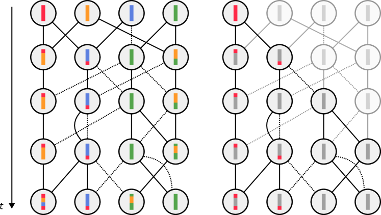
Figure 2: Illustration of the Wright–Fisher model with recombination. A line is drawn between each individual and its parents. It is dotted if no genetic material is inherited from this parent. The right panel focuses on the genetic material left by the red individual. Note that each individual only carries an interval before the first reproduction event involving two descendants of the focal ancestor.

In this work, we consider a simpler but related problem. Fix a focal ancestor, and say that its chromosome is red. We trace the individuals in the population that have inherited some genetic material from this focal ancestor, that is, the set of individuals that have some red on their chromosome as well as the location of the red color. To recover the branching approximation that we study, consider an individual in the population at some generation $t$ carrying a red interval $I$. Its offspring size distribution is

$$\mathrm{Binomial}\Big{(}N,\frac{2}{N}\big{(}1+o_{N}(1)\big{)}\Big{)}\xrightarrow[\>N\to\infty\>]{\>\>}\mathrm{Poisson}(2).$$

Each of these children has another parent in the population. As long as the number of individuals with a red piece of chromosome is small compared to $N$, this other parent does not have any red part on its chromosome.

Therefore, there are only four possible outcomes for each child:

• With probability $1-R/N$ no recombination occurs and

  • with probability $1/2$ it inherits $I$;

  • with probability $1/2$ the interval $I$ is lost.

• With probability $R/N$ a recombination occurs and

  • if $U\not\in I$ the interval $I$ is transmitted or lost with probability $1/2$;

  • if $U\in I$, the child inherits the subinterval of $I$ to the left or to the right of $U$ with probability $1/2$.

By combining the previous cases, we recover that the number of descendants that carry some red of an individual with red interval $I$ is approximately distributed as a $\mathrm{Poisson}\big{(}1+\tfrac{|I|}{N}\big{)}$ r.v., and that the probability of inheriting a fragmented interval is

$$r_{N}(I)=\frac{2|I|/N}{1+|I|{N}}.$$

This is the description of the branching process with recombination.

2.3 Limiting behavior

Let $\mathbf{P}_{R}$ denote the distribution of the branching process with recombination started from a single individual with interval $(0,R)$. The following asymptotic expression for the survival probability of this process was already derived in [3].

Proposition 1 ([3]).

Let $Z_{N}$ denote the population size at generation $N$ in the branching process with recombination. The limit

$$\lim_{N\to\infty}\frac{\mathbf{P}_{R}(Z_{N}>0)}{N}$$

exists. Moreover it fulfills

$$\lim_{R\to\infty}\lim_{N\to\infty}\frac{R\,\mathbf{P}_{R}(Z_{N}>0)}{N\log R}=1.$$

Let $T_{N}$ denote the set of individuals at generation $N$ in the branching process with recombination. For an individual $u\in T_{N}$, we denote by $I_{u}$ the interval that it carries. For $u,v\in T_{N}$, let $d_{T}(u,v)$ denote the genealogical distance between $u$ and $v$, that is, the number of generations that need to be traced backward in time before $u$ and $v$ find a common ancestor.

Our first result provides the joint limit of the interval lengths and of the genealogy of the population. To derive this limit, we will envision the population as a marked metric measure space and work with the marked Gromov-weak topology [10]. The definition of this topology is recalled in Section 4.1.

Let us consider the measure $\mu_{N}$ on $T_{N}\times\mathbb{R}_{+}$ defined as

$$\mu_{N}=\sum_{u\in T_{N}}\delta_{(u,|I_{u}|)}.$$

The triple $[T_{N},d_{T},\mu_{N}]$ is the marked metric measure space corresponding to the branching process with recombination. Let us finally define the rescaling

$$\forall x\in[0,1],\quad F_{R}(x)=\frac{\log\big{(}(R-1)x+1\big{)}}{\log R},\quad F^{-1}_{R}(x)=\frac{R^{x}-1}{R-1}$$ (1)

and define the rescaled distance as

$$\forall u,v\in T_{N},\quad\bar{d}_{N}^{R}=1-F_{R}\big{(}1-\tfrac{d_{T}(u,v)}{N}\big{)}$$

which is the distance obtained by rescaling time according to $F_{R}$.

Theorem 1.

Fix $t>0$. Conditional on survival at time $\lfloor Nt\rfloor$ the following limit holds in distribution for the marked Gromov-weak topology,

$$\lim_{R\to\infty}\lim_{N\to\infty}\Big{[}T_{\lfloor Nt\rfloor},\bar{d}_{\lfloor Nt\rfloor}^{R},\frac{\mu_{\lfloor Nt\rfloor}}{tN\log R}\Big{]}=\big{[}(0,Y),d_{P},\operatorname{Leb}\otimes\mathrm{Exp}(t)\big{]}$$

where $[(0,Y),d_{P}]$ is a Brownian coalescent point process, and $\mathrm{Exp}(t)$ is the exponential distribution with mean $1/t$.

A stronger version of this result is proved in Section 6.3. Let us now briefly discuss several consequences of the previous result.

Convergence of the empirical measure.

As mentioned in the introduction, the branching process at hand is naturally driven to criticality through recombination. Recall that if the offspring distribution of a (standard) critical branching processes has finite second moment, the celebrated Yaglom law states that conditional on survival up to time $Nt$, the rescaled population size $Z_{\lfloor Nt\rfloor}/N$ converges to an exponential random variable. In contrast, the convergence of $\frac{\mu_{\lfloor Nt\rfloor}}{tN\log R}$ entails that the rescaled population size at time $Nt$ converges to an exponential random variable, but the population size is of order $N\log R$ instead of $N$. In words, the local supercritical character of the process translates into an extra $\log R$ factor for the population size.

Secondly, the convergence of the random measure $\frac{\mu_{\lfloor Nt\rfloor}}{tN\log R}$ also implies that the length of the interval carried by a typical individual in the population is exponentially distributed with mean $1/t$. Since the limiting random measure is deterministic, the intervals carried by $k$ typical individuals in the populations are independent (propagation of chaos). Note that, although the length of the initial interval $R$ goes to infinity, the intervals at any finite time $t$ remain of finite length. This phenomenon is usually referred to as coming down from infinity. In our work, it originates from the existence of an entrance law at infinity for the spine, which turns out to be connected to the existence of such entrance laws for positive self-similar Markov processes with negative index of self-similarity [5, 6].

Convergence of the genealogy.

Let us first comment on the rescaling $F_{R}$. Although the expression of $F_{R}$ appears a bit daunting at first, it essentially boils down to first rescaling time by $N$ (as expected), and then measuring time from the origin in the log-scale. The first consequence is that the genealogy of the population in the natural scale (that is, if we only rescale time by $N$) converges to a star tree so that the genealogy becomes indistinguishable from the one of a supercritical branching process at the limit.

A second consequence of this result is that, after rescaling time according to $F_{R}$, the genealogy of the branching process with recombination converges to a limiting metric space named the Brownian coalescent point process (CPP). It is constructed out of a Poisson point process $P$ on $(0,\infty)\times(0,1)$ with intensity $\mathrm{d}t\otimes\frac{1}{x^{2}}\mathrm{d}x$. Let

$$\forall x\leq y,\quad d_{P}(x,y)=\sup\{z:(t,z)\in P,\,x\leq t\leq y\}.$$

The Brownian CPP is the random metric space $[(0,Y),d_{P}]$, where $Y$ is an exponential r.v. with mean $1$, independent of $P$, see Figure 3 for a graphical construction. It corresponds to the limit of the genealogy of a critical Galton–Watson process with finite variance [39].

Chromosomic distance.

The previous result provides a complete description of the interval lengths in the population, but does not provide any insight into their distribution over $(0,R)$. We will encode the latter information by picking a reference point belonging to each interval in the population and considering the usual distance on the real line between these points. More precisely, for each $u\in T_{N}$, pick a reference point $M_{u}$ uniformly on $I_{u}$. We define a new metric

$$\forall u,v\in T_{N},\qquad D_{N}(u,v)=|M_{u}-M_{v}|.$$

We will refer to the $D_{N}$ as the chromosomic distance.

The quadruple $[T_{N},d_{N},D_{N},\mu_{N}]$ can be seen as a random “bi-metric” measure space with marks. We can define a straightforward extension of the marked Gromov-weak topology for such objects, see the end of Section 4.1. The correct rescaling for $D_{N}$ is to set

$$\forall u,v\in T_{N},\quad\bar{D}_{N}^{R}=\frac{\log D_{N}\vee 2}{\log R}$$

In Section 6.3, we prove the following refinement of Theorem 1.

Theorem 2.

Fix $t>0$. Conditional on survival of the process at $\lfloor tN\rfloor$, the following limit holds in distribution for the marked Gromov-weak topology,

$$\lim_{R\to\infty}\lim_{N\to\infty}\Big{[}T_{\lfloor Nt\rfloor},\bar{d}_{\lfloor Nt\rfloor}^{R},\bar{D}_{\lfloor Nt\rfloor}^{R},\frac{\mu_{\lfloor tN\rfloor}}{tN\log R}\Big{]}=\big{[}(0,Y),d_{P},d_{P},\operatorname{Leb}\otimes\mathrm{Exp}(t)\big{]}$$

where $[(0,Y),d_{P}]$ is a Brownian coalescent point process, and $\mathrm{Exp}(t)$ is the exponential distribution with mean $1/t$.

It is important to note that, in the limit, the two metrics coincide. This result is quite interesting from a biological point of view. It shows that there is a correspondence between the genealogical distance between two individuals, and the chromosomic distance between the genetic material that they carry. Indeed, the latter two quantities are correlated: two individuals inherit intervals that are subsets of the interval carried by their most-recent common ancestor. If this ancestor is recent, its interval is smaller, and so is their chromosomic distance. Our result shows that, in the limit, the two distances become identical when considered on the right scale. This result is illustrated in Figure 3.

Figure 3: Top: simulation of a Brownian CPP. The black vertical lines represent to the atoms of $P$, and the corresponding tree is pictured in grey. Bottom: geometry of the blocks of ancestral material corresponding to the top CPP. Each block is represented by a black stripe. The correspondence between the blocks and the tree are shown for some blocks by grey segments joining the two. The distance between two consecutive stripes is the logarithm of their distance on the chromosome. Note that this induces a strong deformation of the intuitive linear scale.

Remark 1.

Define the point process

$$\vartheta=\sum_{x\geq 0}\operatorname{Leb}(\{y\in(0,Y):d_{P}(0,y)=x\})\delta_{x}$$

which corresponds to the CPP tree “viewed from the individual with the left-most interval”. Using elementary properties of Poisson point processes shows that $\vartheta$ can also be written as

$$\vartheta=\sum_{(x_{i},y_{i})\in\mathcal{P}}y_{i}\delta_{x_{i}}$$

where $\mathcal{P}$ is a Poisson point process on $(0,\infty)\times(0,\infty)$ with intensity $\frac{1}{x^{2}}e^{-x/y}\mathrm{d}x\mathrm{d}y$.

The same expression was obtained in [28, Theorem 1.5] to describe the set of loci that share the same ancestor as the left-most locus in the fixed haplotype of a Wright–Fisher model with recombination, under a limiting regime similar to ours. This connection is quite surprising. We are considering a branching approximation where all intervals belong to distinct individuals and its chromosome carries at most one block of ancestral genome, whereas in [28] all intervals belong to a single chromosome, which has reached fixation in the population.

3 The $k$-spine tree

3.1 The many-to-few formula

The objective of this first section is to introduce the $k$-spine tree and state our many-to-few formula, that relates the expression of the polynomials of a branching process to the $k$-spine tree. All the random variables introduced here are more formally defined in the forthcoming sections, where the proof of the many-to-few formula is carried out. A formal statement of our result requires some preliminary notation.

Assumption and notation.

Consider a Polish space $(E,d_{E})$, and a collection $(\Xi(x);\,x\in E)$ of random point measures on $E$. This collection can be used to construct a branching process with type space $E$, such that the atoms of a realization of $\Xi(x)$ provide the types of the children of an individual with type $x$. The distribution of the resulting branching process is denoted by $\mathbf{P}_{x}$.

Let $K(x)$ denote the number of atoms of $\Xi(x)$, and set

$$\pi(x,k)=\mathbb{P}(K(x)=k)$$

for the distribution of $K(x)$. The $n$-th factorial moment of $K(x)$ is denoted by $m_{n}(x)$, that is,

$$m_{k}(x)\coloneqq\mathbb{E}\Big{[}K(x)^{(n)}\Big{]},$$

$$m(x)\coloneqq m_{1}(x)=\mathbb{E}[K(x)],$$

where we have used the notation $k^{(n)}$ for the $n$-th descending factorial of $k$,

$$k^{(n)}=k(k-1)\dots(k-n+1).$$

Our results are more easily formulated under the assumption that, conditional on $K(x)$, the locations of the atoms are i.i.d. with distribution $p(x,\cdot)$. That is, we assume that

$$\Xi(x)=\sum_{i=1}^{K(x)}\delta_{\xi_{i}(x)}$$

where $(\xi_{i}(x);\,i\geq 1)$ is an i.i.d. sequence distributed as $p(x,\cdot)$ and is independent of $K(x)$. We make the further simplifying assumption that all distributions $p(x,\cdot)$ have a density w.r.t. some common measure $\Lambda$ on $E$. With a slight abuse of notation, the density of $p(x,\cdot)$ is denoted by $(p(x,y);\,y\in E)$.

Harmonic function.

We say that a map $h\colon E\to[0,\infty)$ is (positive) harmonic if

$$\forall x\in E,\quad h(x)=\mathbb{E}[\langle\Xi(x),h\rangle],$$

where we used the notation $\langle\mu,f\rangle=\int f\mathrm{d}\mu$, see for instance [7]. A harmonic function can be used to define a new probability kernel on $E$, defined as

$$\forall x,y\in E,\quad q(x,y)=\frac{m(x)h(y)p(x,y)}{h(x)}.$$ (2)

The fact that this is a probability measure follows from the harmonicity of $h$.

The $k$-spine tree.

We are now ready to define the $k$-spine tree. Let $\nu=(\nu_{n};\,n\in\{0,\dots,N-1\})$ be a probability distribution and let $(W_{1},\dots,W_{k-1})$ be i.i.d. random variables with distribution $\nu$. Define

$$\forall i\leq j,\quad d_{T}(i,j)=d_{T}(j,i)=\max\{N-W_{i},\dots,N-W_{j-1}\}.$$

There is a unique tree with $k$ leaves labeled by $\{1,\dots,k\}$ such that the tree distance between the leaves is $d_{T}$. We denote it by $S$ and call it the $\nu$-CPP tree. This tree is constructed inductively by grafting a branch of length $N-W_{i}$ on the tree constructed at step $i$, as illustrated in Figure 4.

We now assign marks on the tree such that along each branch of the tree, marks evolve according to a Markov chain with transition kernel $(q(x,y);\,x,y\in E)$ defined in (2). More formally construct a collection of processes $(X_{1},\dots,X_{k})$ such that

• the process $(X_{1}(n);\,n\geq 0)$ is a Markov chain with transition $(q(x,y);\,x,y\in E)$ started from $x$;

• conditional on $(X_{1},\dots,X_{i})$,

  $$\forall n\geq 0,\quad X_{i+1}(n)=\begin{cases}X_{i}(n)&\text{if $n<W_{i}$}\\ X^{\prime}(n-W_{i})&\text{if $n\geq W_{i}$}\end{cases}$$

  for some independent Markov chain $X^{\prime}$ with transition $(q(x,y);\,x,y\in E)$ started from $X_{i}(W_{i})$.

By thinking of $(X_{i}(n);\,n\geq 0)$ as giving the sequence of marks along the branch of $S$ starting from the root and going to the $i$-th leaf, we can assign to each vertex $u\in S$ a mark $Y_{u}$.

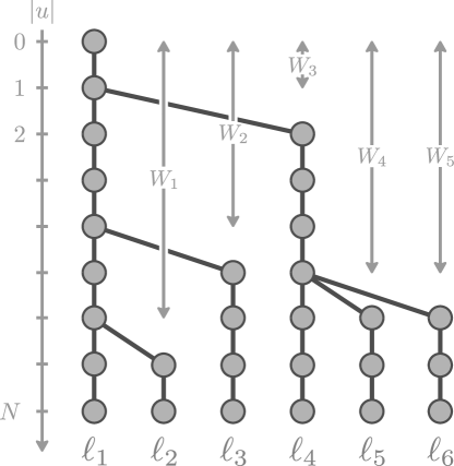
Figure 4: Illustration of the construction of a CPP tree. The vector $(W_{1},\dots,W_{k-1})$ branching times between successive leaves. In this example, this vector is $(6,4,1,5,5)$. The tree is recovered from these times by grafting for each $i$ a branch of length $N-W_{i}$ to the right-most vertex of the tree at generation $W_{i}$.

Definition 1.

The $k$-spine tree is the random marked tree $[S,(Y_{u};\,u\in S)]$ encoded by the variables $(W_{1},\dots,W_{k-1})$ and $(X_{1},\dots,X_{k})$. The distribution of the latter variables is denoted by $\mathbf{Q}^{k,N}_{x}$.

We are now ready to state our many-to-few formula. It can be described informally as follows. Suppose that the branching process with law $\mathbf{P}_{x}$ is biased by the $k$-th factorial moment of its size at generation $N$ and that $k$ individuals are chosen uniformly for that generation. Then the law of the subtree spanned by these individuals is $\mathbf{Q}^{k,N}_{x}$ biased by a random factor $\Delta_{k}$ that can be expressed as

$$\Delta_{k}=\prod_{\begin{subarray}{c}u\in S\\ d_{u}>1\end{subarray}}\Big{(}\frac{h(Y_{u})}{N\nu_{|u|}}\Big{)}^{d_{u}-1}\frac{m_{d_{u}}(Y_{u})}{d_{u}!\,m(Y_{u})^{d_{u}}}\cdot\prod_{i=1}^{k}\frac{1}{h(X_{i}(N))},$$ (3)

where $d_{u}$ denotes the degree of a vertex $u\in S$ and $Y_{u}$ its mark. Note that the left product in (3) has at most $k-1$ terms, which correspond to the branch points in $S$.

Lemma 1.

Assume that for every $x\in E$, the offspring number $K(x)$ is Poisson (for some given parameter $\lambda(x)>0$ that may depend on $x$). Then

$$\Delta_{k}=\prod_{\begin{subarray}{c}u\in S\\ d_{u}>1\end{subarray}}\Big{(}\frac{h(Y_{u})}{N\nu_{|u|}}\Big{)}^{d_{u}-1}\frac{1}{d_{u}!}\cdot\prod_{i=1}^{k}\frac{1}{h(X_{i}(N))}.$$

Proof.

This simply follows from the well known fact that the $k$-th factorial moment of a Poisson random variable with parameter $\lambda>0$ is $\lambda^{k}$. ∎

Finally, let $T_{N}$ denote the labels of the $N$-th generation of a branching process with distribution $\mathbf{P}_{x}$, for $u\in T_{N}$ let $X_{u}$ denote its type, and let $d_{T}$ denote the tree distance on $T_{N}$.

Proposition 2 (Many-to-few).

For any test function $\varphi$,

$$\mathbf{P}_{x}\Big{[}\sum_{\begin{subarray}{c}(v_{1},\dots,v_{k})\in T_{N}\\ v_{1}\neq\dots\neq v_{k}\end{subarray}}\varphi\big{(}d_{T}(v_{i},v_{j}),X_{v_{i}};\,i,j\leq k\big{)}\Big{]}\\ =h(x)N^{k-1}k!\,\mathbf{Q}^{k,N}_{x}\Big{[}\Delta_{k}\cdot\varphi\big{(}d_{T}(\sigma_{i},\sigma_{j}),X_{\sigma_{i}}(N);\,i,j\leq k\big{)}\Big{]}$$

where $\sigma$ is an independent uniform permutation of $\{1,\dots,k\}$.

Remark 2.

1. In our construction of the $k$-spine, the distribution of the tree is independent of the marking. The term $\Delta_{k}$ captures the interplay between the genealogy and the types as a function of the marking at “topological” points.

2. Compare Proposition 2 to the many-to-few formula in [22]. Both expressions relate the distribution of a $k$-sample from the branching process (l.h.s. of the equality) to that of a simpler $k$-spine tree (r.h.s. of the equality) at the expense of a bias term, here denoted by $\Delta_{k}$.

3. In [22], the $k$-spine tree only depends on the moments of the reproduction law. Our formulation has one extra degree of freedom, since the $k$-spine tree is constructed out of an a priori genealogy, the $\nu$-CPP tree.

4. In many situations, including the model at hand, the bias term in [22] becomes degenerate in the limit so that the distribution of the limiting genealogy is singular with respect to that of the original $k$-spine tree. For instance, for near-critical processes conditioned on survival at generation $N$, the first split time of the $k$-spine tree in [22, Section 8] remains of order $1$, whereas the most-recent common ancestor of the whole population is known to live at a time of order $N$. In contrast, one advantage of our approach is that $\nu$ can be well-chosen so that the bias $\Delta_{k}$ converges to a non-degenerate limit. This amounts to finding a good ansatz for the limiting genealogy. In our example this ansatz is given in (17), and the limit of the bias $\Delta_{k}$ is independent of the genealogy. This indicates that the limit of the genealogy does not depend on the types in the population.

The rest of the section is dedicated to the proof of the many-to-few formula. Our strategy to prove this result is to define a new tree with distribution $\bar{\mathbf{Q}}^{k,N}_{x}$ by grafting on the $k$-spine tree independent subtrees distributed as the original branching process. The many-to-few formula will then follow from the more precise spinal decomposition theorem, which states that $\bar{\mathbf{Q}}^{k,N}_{x}$ and $\mathbf{P}_{x}$ are connected through the random change of measure $\Delta_{k}$. It is proved in Section 3.4. The remaining sections provide a rigorous construction of the measures $\mathbf{P}_{x}$ and $\bar{\mathbf{Q}}_{x}^{k,N}$ and the proof of the spinal decomposition theorem.

3.2 Tree construction of the branching process

Let us recall some common notation on trees.

Trees.

Following the usual Ulam–Harris labeling convention, all trees will be encoded as subsets of

$$\mathscr{U}\coloneqq\{\varnothing\}\cup\bigcup_{n\geq 1}\mathbb{N}^{n}.$$

Let us consider an element $u=(u(1),\dots,u(n))\in\mathscr{U}$. We denote by $|u|=n$ its length, interpreted as the generation of $u$. Moreover, its $i$-th child is denoted by

$$ui\coloneqq(u,i)=(u(1),\dots,u(n),i),$$

and its ancestor in the previous generation as

$$\overleftarrow{u}\coloneqq(u(1),\dots,u(n-1)).$$

The set $\mathscr{U}$ is naturally endowed with a partial order $\preceq$, where $u\preceq v$ if $u$ is an ancestor of $v$, that is,

$$u\preceq v\iff\forall i\leq|u|,\;u(i)=v(i).$$

The most-recent common ancestor of $u$ and $v$ can then be defined as

$$u\wedge v\coloneqq\max\{w:w\preceq u\text{ and }w\preceq v\}.$$

In the tree interpretation of $\mathscr{U}$, we can define a metric $d_{T}$ corresponding to the graph distance as

$$\forall u,v\in\mathscr{U},\quad d_{T}(u,v)\coloneqq\operatorname{Card}\{w:u\wedge v\preceq w\prec u\}+\operatorname{Card}\{w:u\wedge v\preceq w\prec v\}.$$

Finally, as a consequence of the Ulam–Harris encoding, trees are planar in the sense that the children of each vertex are endowed with a total order. Accordingly let us denote by $\leq$ the lexicographical order on $\mathscr{U}$, which we will call the planar order. Note that $\leq$ extends $\preceq$.

A subset $\tau\subseteq\mathscr{U}$ is called a tree if

1. $\varnothing\in\tau$;

2. if, for some $j$, $uj\in\tau$, then $u\in\tau$;

3. for any $u\in\tau$, there exists $k_{u}\in\mathbb{N}$ such that

   $$ui\in\tau\iff i\leq k_{u},$$

   where $k_{u}$ is the number of children of $u$, also called the (out-)degree of $u$.

The set of all trees is denoted by $\Omega$. For a tree $\tau\in\Omega$, define its restriction to the $n$-th generation as

$$\tau_{n}=\{u\in\tau:|u|=n\}$$

and that to the first $n$ generations as

$$\tau_{[n]}=\{u\in\tau:|u|\leq n\}=\bigcup_{i=1}^{n}\tau_{i}.$$

Furthermore, let us denote by $\Omega_{n}$ the set of trees of height at most $n$, where the height of a tree is defined as the generation of the oldest individual in the tree.

Marked trees and definition of $\mathbf{P}_{x}$.

A marked tree is a tree $\tau\in\Omega$ with a collection $(x_{u};\,u\in\tau)$ of marks with values in $E$. Let us define a random marked tree $[T,(X_{u};\,u\in T)]$ inductively as follows, that corresponds to the branching process with offspring reproduction point processes $(\Xi(x);\,x\in E)$.

Start from a single individual $\varnothing$ with mark $X_{\varnothing}=x$. Conditional on the first $n$ generations $T_{[n]}$ and their marks $(X_{u};\,u\in T_{[n]})$, consider a collection of independent point processes $(\Xi_{u};\,u\in T_{n})$, where

$$\Xi_{u}\sim\Xi(X_{u}).$$

Let us write

$$\Xi_{u}=\sum_{i=1}^{K_{u}}\delta_{\xi_{ui}}$$

for the atoms of $\Xi_{u}$. Then define the next generation as

$$T_{[n+1]}=T_{[n]}\cup\{ui:u\in T_{n},i\leq K_{u}\},$$

with marks given by

$$\forall ui\in T_{n+1},\quad X_{ui}=\xi_{ui}.$$

Let $T=\cup_{n\geq 1}T_{n}$ be the whole tree, and define define $\mathbf{P}_{x}$ as the law of the random marked tree $[T,(X_{u};\,u\in T)]$ obtained through the previous procedure, and $\mathbf{P}^{N}_{x}$ the law of its restriction to the first $N$ generations.

3.3 Ultrametric trees

From now on, we consider a fixed, focal generation $N$. In this section we construct the measure $\bar{\mathbf{Q}}^{k,N}_{x}$ obtained by grafting some independent subtrees on the $k$-spine tree. This construction relies on the notion of (discrete) ultrametric trees.

Ultrametric trees.

A tree $\tau\in\Omega_{N}$ with height $N$ is called ultrametric if all of its leaves lie at height $N$, that is

$$\forall u\in\tau,\quad k_{u}=0\implies|u|=N.$$

The set of all ultrametric trees of height $N$ with $k$ leaves is denoted by $\mathbb{U}^{k,N}$. For $\tau\in\mathbb{U}^{k,N}$, let us denote by $(\ell_{1},\dots,\ell_{k})$ the leaves of $\tau$ in lexicographical order, that is, such that

$$\ell_{1}\leq\dots\leq\ell_{k}.$$

The previous description of an ultrametric tree as an element of $\Omega_{N}$ is not suitable to describe the large $N$ limit of the $k$-spine tree. To derive such a limit, we need to encode elements of $\mathbb{U}^{k,N}$ as a sequence $(g_{1},\dots,g_{k-1})$ giving the branch times between successive leaves in the tree. This construction is sometimes referred to as a coalescent point process (CPP) [39, 29].

More precisely, define the map

$$\Phi\colon\begin{cases}\mathbb{U}^{k,N}\to\{0,\dots,N-1\}^{k-1}\\ \tau\mapsto\big{(}|\ell_{1}\wedge\ell_{2}|,\dots,|\ell_{k-1}\wedge\ell_{k}|\big{)}.\end{cases}$$

The following straightforward result shows that the tree $\tau$ can be recovered from the vector of coalescence times $\Phi(\tau)$.

Lemma 2.

The map $\Phi$ is a bijection from the set of ultrametric trees $\mathbb{U}^{k,N}$ to the set of vectors $\{0,\dots,N-1\}^{k-1}$.

The $k$-spine tree.

Let $(W_{1},\dots,W_{k-1})$ and $(X_{1},\dots,X_{k})$ have distribution $\mathbf{Q}^{k,N}_{x}$. We formally define the $\nu$-CPP tree illustrated in Figure 4 as the random tree $S\coloneqq\Phi^{-1}(W_{1},\dots,W_{k-1})$. Note that the CPP tree associated to the uniform distribution is uniform on $\mathbb{U}^{k,N}$. The processes $(X_{1},\dots,X_{k})$ can now be used to construct a collection of marks $(Y_{u};\,u\in S)$ as follows. Each $u\in S$ is of the form

$$u=(\ell_{i}(1),\dots,\ell_{i}(n))$$

for some leaf $\ell_{i}$ and $n\leq N$. Define the mark of such a $u$ as

$$Y_{u}\coloneqq X_{i}(n).$$

(It is not hard to see that $Y_{u}$ is well-defined in that it does not depend on the choice of $\ell_{i}$ if $u$ is ancestral to several leaves.) The marked tree $[S,(Y_{u})]$ is the $k$-spine tree encoded by the r.v. $(W_{1},\dots,W_{k-1})$ and $(X_{1},\dots,X_{k})$.

Construction of $\bar{\mathbf{Q}}^{k,N}_{x}$.

Let $[S,(Y_{u})]$ be the $k$-spine tree constructed above. We attach to $S$ some subtrees distributed as $\mathbf{P}_{x}$ to define a larger marked tree $[T,(X_{u})]$. This yields a random tree with $k$ spines originated from the $k$ leaves of $S$ at generation $N$. The distribution of these random variables will be denoted by $\bar{\mathbf{Q}}^{k,N}_{x}$.

To construct $T$ from the spine, we first specify the number of subtrees that need to be attached to each vertex $u$ of the spine. We will distinguish the degree of a vertex in $S$ and that in the larger tree $T$. We denote by $d_{u}$ the number of children in $S$ of $u$. (The degree of $u$ in $T$ will be denoted by $k_{u}$ as previously.) We work conditional on $[S,(Y_{u})]$ and assume them to be fixed. Let $(K_{u};\,u\in S,|u|<N)$ be independent variables such that $K_{u}$ has the distribution of $K(Y_{u})$, biased by its $d_{u}$-th factorial moment. That is,

$$\mathbb{P}(K_{u}=k)=\frac{k^{(d_{u})}}{m_{d_{u}}(Y_{u})}\pi(Y_{u},k).$$ (4)

Among the $K_{u}$ children of $u$ in $T$, $d_{u}$ are distinguished as they correspond to the children of $u$ in $S$. Let $C_{u1}<\dots<C_{ud_{u}}$ be the labels of these distinguished children, and let us assume that they are uniformly chosen among the $\binom{K_{u}}{d_{u}}$ possibilities. We can now define the subtree corresponding to $S$ in the larger tree $T$ by an inductive relabelling of the nodes. For $u\in S$, define $\Psi(u)$ inductively as follows

$$\Psi(\varnothing)=\varnothing,\quad\Psi(ui)=\Psi(u)C_{ui},$$

with corresponding marks

$$X_{\Psi(u)}=Y_{u}.$$

Finally, let us attach the subtrees to $[S,(Y_{u})]$. For $u\in S$, consider a sequence $[T_{ui},(X_{ui,v};\,v);\,i\geq 1]$ of i.i.d. marked trees with the original distribution $\mathbf{P}_{X_{ui,\varnothing}}$, but with random initial mark $X_{ui,\varnothing}$ distributed as $p(Y_{u},\cdot)$. The final tree $T$ is defined as

$$T=\bigcup_{\begin{subarray}{c}u\in S\\ |u|<N\end{subarray}}\bigcup_{\begin{subarray}{c}i\in[K_{u}]\\ ui\notin\Psi(S)\end{subarray}}\Psi(u)iT_{ui},$$

and for $v\in T_{ui}$, the mark of $\Psi(u)iv$ is

$$X_{\Psi(u)iv}=X_{ui,v}.$$

Informally, for each of the $K_{u}-d_{u}$ children of $u$ that are not in $S$, we realize one step of the Markov chain with kernel $(p(x,y);\,x,y\in E)$ and then attach a whole subtree $T_{ui}$ to that child.

The resulting tree $T$ has $k$ distinguished leaves, $\Psi(\ell_{1}),\dots,\Psi(\ell_{k})$, corresponding to the $k$ leaves of $S$. Let us finally define

$$\forall i\leq k,\quad V_{i}=\Psi(\ell_{\sigma_{i}})$$

for an independent uniform permutation $\sigma$ of $\{1,\dots,k\}$. The distribution of the triple $[T_{[N]},(X_{u}),(V_{i})]$ is denoted by $\bar{\mathbf{Q}}^{k,N}_{x}$, where $T_{[N]}$ is the restriction of $T$ to the first $N$ generations.

3.4 The spinal decomposition theorem

Our final objective in this section is to connect $\mathbf{P}_{x}$ and $\bar{\mathbf{Q}}^{k,N}_{x}$ to derive our many-to-few formula. We assume $\nu_{n}>0$ for all $n\in\{0,\dots,N-1\}$. Recall the expression of $\Delta_{k}$ from (3). Our spinal decomposition theorem states that, if $\mathbf{P}_{x}$ is biased by the $k$-th factorial moment of its size at generation $N$ and $k$ uniformly chosen individuals $(V_{1},\dots,V_{k})$ are distinguished from that generation, the corresponding marked tree $[T_{N},(X_{u}),(V_{i})]$ is distributed as $\bar{\mathbf{Q}}^{k,N}_{x}$ biased by $\Delta_{k}$.

Theorem 3 (Spinal decomposition).

Consider a tree $\tau$ with height $N$ and $k$ distinct vertices $(v_{1},\dots,v_{k})\in\tau_{N}$. Let $h$ be a harmonic function for the branching process with law $(\mathbf{P}_{x};\,x\in E)$. Then, for any test function $\varphi$, we have

$$\mathbf{P}^{N}_{x}\Big{[}\mathbf{1}_{T=\tau}\varphi(X_{u};\,u\in\tau)\Big{]}=h(x)N^{k-1}k!\,\bar{\mathbf{Q}}^{k,N}_{x}\Big{[}\Delta_{k}\cdot\mathbf{1}_{T=\tau}\mathbf{1}_{V_{1}=v_{1},\dots,V_{k}=v_{k}}\varphi(X_{u};\,u\in\tau)\Big{]}.$$

Proof.

It is enough to prove the result for the uniform CPP by noting that $\prod_{u\in S}\frac{1}{N\nu_{u}}$ is the Radon–Nykodim derivative of the uniform CPP with respect to the $\nu$-CPP.

The natural state space for $\mathbf{P}^{N}_{x}$ is the space of all marked trees with height at most $N$, that is,

$$\bigcup_{\tau\in\Omega_{N}}\{\tau\}\times E^{\tau}.$$

Using that the offspring distribution on $E$ has a density w.r.t. some measure $\Lambda$, it is clear that $\mathbf{P}^{N}_{x}$ has a density w.r.t. a dominating measure defined as

$$\Lambda^{N}\Big{(}\bigcup_{\tau\in\Omega_{N}}\{\tau\}\times\prod_{u\in\tau}B_{u}\Big{)}=\sum_{\tau\in\Omega_{N}}\prod_{u\in\tau}\Lambda(B_{u})$$

which is given by

$$P_{x}^{N}(\tau,(x_{u}))=\prod_{\begin{subarray}{c}u\in\tau\\ |u|<n\end{subarray}}\pi(x_{u},k_{u})\prod_{i=1}^{k_{u}}p(x_{u},x_{ui})$$ (5)

where $k_{u}$ stands for the number of children of $u$.

Let $\mathbf{s}$ denote the subtree spanned by $(v_{1},\dots,v_{k})$, that is

$$\mathbf{s}=\bigcup_{i=1}^{k}\{w:w\preceq v_{i}\}.$$

We can decompose (5) into a product on $\mathbf{s}$ and on the subtrees attached to $\mathbf{s}$. The branching property shows that

$$P_{x}^{N}(\tau,(x_{u})) =\prod_{\begin{subarray}{c}u\in\mathbf{s}\\ |u|<N\end{subarray}}\pi(x_{u},k_{u})\bigg{[}\prod_{\begin{subarray}{c}i\in[k_{u}]\\ ui\notin\mathbf{s}\end{subarray}}p(x_{u},x_{ui})P_{x_{ui}}\big{(}\tau_{ui},(x_{uiv})_{v}\big{)}\times\prod_{\begin{subarray}{c}i\in[k_{u}]\\ ui\in\mathbf{s}\end{subarray}}p(x_{u},x_{ui})\bigg{]}$$

$$=\bigg{[}\prod_{\begin{subarray}{c}u\in\mathbf{s}\\ |u|<N\end{subarray}}\pi(x_{u},k_{u})\prod_{\begin{subarray}{c}i\in[k_{u}]\\ ui\notin\mathbf{s}\end{subarray}}p(x_{u},x_{ui})P_{x_{ui}}(\tau_{ui},(x_{uiv})_{v})\bigg{]}\prod_{u\in\mathbf{s}\setminus\{\varnothing\}}p(x_{\overleftarrow{u}},x_{u}).$$

For $u\in\mathbf{s}$, let $d_{u}$ denote the number of children of $u$ that belong to $\mathbf{s}$, that is,

$$d_{u}=\operatorname{Card}\{i:ui\in\mathbf{s}\}.$$

Let us make the following change in the previous equality

$$\pi(x_{u},k_{u})=\frac{1}{k_{u}^{(d_{u})}}\cdot\frac{k_{u}^{(d_{u})}\pi(x_{u},k_{u})}{m_{d_{u}}(x_{u})}\cdot m_{d_{u}}(x_{u}).$$

Let us also write the second term in the product as

$$\prod_{u\in\mathbf{s}\setminus\{\varnothing\}}p(x_{\overleftarrow{u}},x_{u}) =\prod_{u\in\mathbf{s}\setminus\{\varnothing\}}\frac{h(x_{u})m(x_{\overleftarrow{u}})p(x_{\overleftarrow{u}},x_{u})}{h(x_{\overleftarrow{u}})}\cdot\frac{h(x_{\overleftarrow{u}})}{m(x_{\overleftarrow{u}})h(x_{u})}$$

$$=\prod_{u\in\mathbf{s}\setminus\{\varnothing\}}q(x_{\overleftarrow{u}},x_{u})\cdot\prod_{\begin{subarray}{c}u\in\mathbf{s}\\ |u|<N\end{subarray}}\frac{h(x_{u})^{d_{u}-1}}{m(x_{u})^{d_{u}}}\cdot\prod_{i=1}^{k}\frac{1}{h(x_{v_{i}})}\cdot h(x_{\varnothing}).$$

Putting both expressions together, we obtain that

$$\frac{1}{h(x_{\varnothing})} P_{x}(\tau,(x_{u}))=\prod_{i=1}^{k}\frac{1}{h(x_{v_{i}})}\prod_{\begin{subarray}{c}u\in\mathbf{s}\\ d_{u}>1\end{subarray}}h(x_{u})^{d_{u}-1}\frac{m_{d_{u}}(x_{u})}{d_{u}!\,m(x_{u})^{d_{u}}}\times\prod_{u\in\mathbf{s}\setminus\{\varnothing\}}q(x_{\overleftarrow{u}},x_{u})$$

$$\times\prod_{\begin{subarray}{c}u\in\mathbf{s}\\ |u|<N\end{subarray}}\bigg{[}\frac{d_{u}!}{k_{u}^{(d_{u})}}\cdot\frac{k_{u}^{(d_{u})}\pi(x_{u},k_{u})}{m_{d_{u}}(x_{u})}\cdot\prod_{ui\notin\mathbf{s}}p(x_{u},x_{ui})P_{x_{ui}}\big{(}\tau_{ui},(x_{uiv})_{v}\big{)}\bigg{]}.$$

The result now follows upon identifying each term in this product. The first term is $\Delta_{k}$. The second term is the density of the marks $(x_{u};\,u\in\mathbf{s})$ along the $k$-spine. The last product is made of three terms. The first is the probability that the $d_{u}$ children of $u$ that belong to $\mathbf{s}$ have a given birth rank. The second is the probability that the final degree of $u$ is $k_{u}$ given that it has $d_{u}$ children in $\mathbf{s}$ (see (4)). The last is the density of the marked trees attached to $u$. The $N^{k-1}k!$ term in the statement of theorem is simply the probability of observing a given ultrametric tree and labeling of the leaves. ∎

Proof of Proposition 2.

Let $\tau$ be some fixed tree and $v_{1},\dots,v_{k}$ be distinct vertices at height $N$ of $\tau$. Using Theorem 3 yields

$$\mathbf{P}^{N}_{x}\Big{[}\mathbf{1}_{T=\tau}\varphi\big{(}d_{T}(v_{i},v_{j}),X_{v_{i}};\,i,j\leq k\big{)}\Big{]}\\ =h(x)N^{k-1}k!\,\bar{\mathbf{Q}}^{k,N}_{x}\Big{[}\Delta_{k}\cdot\mathbf{1}_{T=\tau}\mathbf{1}_{V_{1}=v_{1},\dots,V_{k}=v_{k}}\varphi\big{(}d_{T}(V_{i},V_{j}),Y_{V_{i}};\,i,j\leq k\big{)}\Big{]}.$$

Summing over all $(v_{1},\dots,v_{k})$ first, then over all $\tau$, and recalling that $V_{i}=\ell_{\sigma_{i}}$ for an independent uniform permutation $\sigma$ of $\{1,\dots,k\}$ proves the result. ∎

4 Convergence of marked branching processes

4.1 The marked Gromov-weak topology

Deriving the scaling limit of the genealogy and types in a branching process requires one to envision it as a random marked metric measure space. In this work we equip the set of all such spaces with the marked Gromov-weak topology [10]. This section is a brief remainder of the basic properties of this topology, a more thorough account can be found in [10, 18]. We do not restrict our attention to trees and try to follow as much as possible the notation in [10], so that some notation in this section might be inconsistent with the rest of the paper.

Let $(E,d_{E})$ be a fixed complete separable metric space, referred to as the mark space. In our application, $E=[0,\infty)$ is endowed with the usual distance on the real line. A marked metric measure space (mmm-space for short) is a triple $[X,d,\mu]$, where $(X,d)$ is a complete separable metric space, and $\mu$ is a finite measure on $X\times E$.

To define a topology on the set of mmm-spaces, for each $k\geq 1$ consider the map

$$R_{k}\colon\begin{cases}(X\times E)^{k}\to\mathbb{R}_{+}^{k^{2}}\times E^{k}\\ \big{(}(x_{i},u_{i});\,i\leq k\big{)}\mapsto\big{(}d(x_{i},x_{j}),u_{i};\,i,j\leq k\big{)}\end{cases}$$

that maps $k$ points in $X\times E$ to the matrix of pairwise distances and vector of marks. We denote by $\nu_{k,X}=\mu^{\otimes k}\circ R_{k}^{-1}$, the $k$-th marked distance matrix distribution of $[X,d,\mu]$, which is the pushforward of $\mu^{\otimes k}$ by the map $R_{k}$. (Note that $\mu$ is not necessarily a probability distribution.) For some $k\geq 1$ and some continuous bounded test function

$$\varphi\colon\mathbb{R}_{+}^{k^{2}}\times E^{k}\to\mathbb{R}$$

let us define a functional

$$\Phi\big{(}X,d,\mu\big{)}=\langle\nu_{k,X},\varphi\rangle.$$ (6)

Functionals of the previous form are called polynomials ($k$ is the degree or order of the polynomial), and the set of all polynomials, obtained by varying $k$ and $\varphi$, is denoted by $\Pi$.

Definition 2.

The marked Gromov-weak topology is the topology on mmm-spaces induced by $\Pi$. A random mmm-space is a r.v. with values in the set of (equivalence classes of) mmm-spaces, endowed with the Gromov-weak topology and the associated Borel $\sigma$-field.

Remark 3.

Formally, the marked Gromov-weak topology should be defined on equivalence classes of mmm-spaces, where two spaces belong to the same class if ​f there is a measure preserving isometry between the supports of their measures that also preserves marks, see [10, Definition 2.1]. This distinction has little consequences in practice so that we often omit it.

There is a unique equivalence class of all mmm-spaces with a null sampling measure, which acts as the null mmm-space and that we denote by $\mathbf{0}$. It follows from the definition of the Gromov-weak topology that a sequence of mmm-spaces $([X_{n},d_{n},\mu_{n}];\,n\geq 1)$ converges to $\mathbf{0}$ if ​f $\mu_{n}(X_{n}\times E)\to 0$. If $[X,d,\mu]$ is a random mmm-space, the expectation of a polynomial evaluated at $[X,d,\mu]$, namely $\mathbb{E}[\Phi(X,d,\mu)]$, is called a moment of $[X,d,\mu]$.

Remark 4 (Polar decomposition).

An mmm-space $[X,d,\mu]\neq\mathbf{0}$ can be seen as a pair $(\bar{\mu},[X,d,\hat{\mu}])$ where $\bar{\mu}=\mu(X\times E)$ is the total mass of $\mu$ and $\hat{\mu}=\mu/\bar{\mu}$ is the renormalized probability measure. This is the so-called polar decomposition of $[X,d,\mu]$ [9]. The space of all polar decompositions is naturally endowed with the product topology, where the space of all probability mmm-spaces is endowed with the more standard marked Gromov-weak topology restricted to probability mmm-spaces [10]. It is not hard to see that the map taking non-null mmm-spaces to their polar decompositions is an homeomorphism.

An important consequence of this remark is that the convergence in distribution of a sequence of mmm-spaces $[X_{n},d_{n},\mu_{n}]$ implies that of $[X_{n},d_{n},\hat{\mu}_{n}]$, provided that the limit mmm-space is a.s. non-null. In particular, for ultrametric spaces, it implies the convergence in distribution of the genealogy of $k$ individuals sampled from $[X_{n},d_{n},\mu_{n}]$ according to $\hat{\mu}_{n}$.

Many properties of the marked Gromov-weak topology are derived in [10] under the further assumption that $\mu$ is a probability measure. Relaxing this assumption to account for finite measures is quite straightforward but requires some caution, as the total mass of $\mu$ can now drift to zero or infinity. In particular, the following result shows that $\Pi$ forms a convergence determining class only when the limit satisfies a moment condition, which is a well-known criterion for a real variable to be identified by its moments, see for instance [14, Theorem 3.3.25]. This result was already stated for metric measure spaces without marks in [9, Lemma 2.7].

Proposition 3.

Suppose that $[X,d,\mu]$ is a random mmm-space verifying

$$\limsup_{p\to\infty}\frac{\mathbb{E}[\mu(X\times E)^{p}]^{1/p}}{p}<\infty.$$ (7)

Then, for a sequence $[X_{n},d_{n},\mu_{n}]$ of random mmm-spaces to converge in distribution for the marked Gromov-weak topology to $[X,d,\mu]$ it is sufficient that

$$\lim_{n\to\infty}\mathbb{E}\big{[}\Phi\big{(}X_{n},d_{n},\mu_{n}\big{)}\big{]}=\mathbb{E}\big{[}\Phi\big{(}X,d,\mu\big{)}\big{]}$$

for all $\Phi\in\Pi$.

Proof.

Let us prove this result carefully. Fix a polynomial $\Phi$ of degree $k$ associated to a non-negative continuous bounded functional $\varphi$. Recall the notation $\bar{\mu}_{n}$ for the total mass of $[X_{n},d_{n},\mu_{n}]$, which is a r.v. with values in $[0,\infty)$, and $\hat{\mu}_{n}=\mu_{n}/\bar{\mu}_{n}$. Introduce a new measure $M_{n}^{\Phi}$ on $[0,\infty)$ such that for any continuous bounded function $f\colon[0,\infty)\to\mathbb{R}$

$$\langle M_{n}^{\Phi},f\rangle=\mathbb{E}[f(\bar{\mu}_{n})\Phi(X_{n},d_{n},\mu_{n})].$$

The key observation is now that, applying Fubini’s theorem, $[X,d,\mu]\mapsto\bar{\mu}^{p}\Phi(X,d,\mu)$ is again a polynomial of the form (6) (of degree $p+k$). Therefore, our assumption entails that, for any integer $p\geq 0$,

$$\int_{0}^{\infty}x^{p}M_{n}^{\Phi}(\mathrm{d}x)=\mathbb{E}[\bar{\mu}_{n}^{p}\Phi(X_{n},d_{n},\mu_{n})]\xrightarrow[\>n\to\infty\>]{\>\>}\mathbb{E}[\bar{\mu}^{p}\Phi(X,d,\mu)]=\int_{0}^{\infty}x^{p}M^{\Phi}(\mathrm{d}x)$$

where we have defined $M^{\Phi}$ is a similar way to $M^{\Phi}_{n}$ using the limiting random variable $[X,d,\mu]$. Now, the usual method of moments on $[0,\infty)$, see for instance [14, Theorem 3.3.26], entails that for any continuous bounded function $f$

$$\mathbb{E}[f(\bar{\mu}_{n})\Phi(X_{n},d_{n},\mu_{n})]=\int_{0}^{\infty}f(x)M_{n}^{\Phi}(\mathrm{d}x)\xrightarrow[\>n\to\infty\>]{\>\>}\int_{0}^{\infty}f(x)M^{\Phi}(\mathrm{d}x)=\mathbb{E}[f(\bar{\mu})\Phi(X,d,\mu)].$$ (8)

We have used that $M^{\Phi}$ fulfills the moment growth condition of [14, Theorem 3.3.26] since

$$\int_{0}^{\infty}x^{p}M^{\Phi}(\mathrm{d}x)\leq\|\varphi\|_{\infty}\mathbb{E}[\mu(X\times E)^{p+k}]$$

and (7) holds. By taking linear combinations, (8) holds for any polynomials, not only non-negative ones.

Let $f\colon[0,\infty)\to\mathbb{R}$ be continuous bounded and have its support bounded away from $0$. Since $x\mapsto f(x)/x^{k}$ is continuous bounded, applying (8) to this map and using that $\Phi(X_{n},d_{n},\mu_{n})=\bar{\mu}_{n}^{k}\Phi(X_{n},d_{n},\hat{\mu}_{n})$ shows

$$\mathbb{E}[f(\bar{\mu}_{n})\Phi(X_{n},d_{n},\hat{\mu}_{n})]\xrightarrow[\>n\to\infty\>]{\>\>}\mathbb{E}[f(\bar{\mu})\Phi(X,d,\hat{\mu})].$$

Standard arguments show that the above convergence also holds for $f(x)=g(x)\mathbf{1}_{\{x\geq\varepsilon\}}$ for any continuous bounded $g$ and $\varepsilon>0$ such that $\mathbb{P}(\bar{\mu}=\varepsilon)=0$. Since [10, Theorem 5] ensures that polynomials are convergence determining on mmm-spaces with a probability sampling measure, we can use [15, Proposition 4.6, Chapter 3] to obtain that for any continuous bounded functional $F$ on the space of mmm-spaces,

$$\mathbb{E}[F(X_{n},d_{n},\mu_{n})\mathbf{1}_{\{\bar{\mu}_{n}\geq\varepsilon\}}]\xrightarrow[\>n\to\infty\>]{\>\>}\mathbb{E}[F(X,d,\mu)\mathbf{1}_{\{\bar{\mu}\geq\varepsilon\}}].$$ (9)

(Here we have applied the result to the polar decomposition of the mmm-space, and used that the polar decomposition defines an homeomorphism.)

To end the proof, we note that by Portmanteau’s theorem

$$\mathbb{P}(\bar{\mu}<\varepsilon)\leq\liminf_{n\to\infty}\mathbb{P}(\bar{\mu}_{n}<\varepsilon)\leq\limsup_{n\to\infty}\mathbb{P}(\bar{\mu}_{n}\leq\varepsilon)\leq\mathbb{P}(\bar{\mu}\leq\varepsilon).$$ (10)

Finally, we write

$$\mathbb{E}[F(X_{n},d_{n},\mu_{n})]=\mathbb{E}[F(X_{n},d_{n},\mu_{n})\mathbf{1}_{\{\bar{\mu}_{n}\geq\varepsilon\}}]+\mathbb{E}[F(X_{n},d_{n},\mu_{n})\mathbf{1}_{\{\bar{\mu}_{n}<\varepsilon\}}]$$

take a limit $n\to\infty$ first, then $\varepsilon\to 0$, and use (9) to estimate the first term and (10) to control the second one to obtain

$$\mathbb{E}[F(X_{n},d_{n},\mu_{n})]\xrightarrow[\>n\to\infty\>]{\>\>}\mathbb{E}[F(X,d,\mu)]$$

which is the desired result. ∎

Bi-metric measure spaces.

The branching process with recombination is naturally endowed with two metrics: the genealogical distance and the chromosomic distance. Therefore, for the purpose of this application only, let us say that $[X,d,D,\mu]$ is a marked bi-metric measure space if both $d$ and $D$ are metric that make $(X,d)$ and $(X,D)$ Polish spaces, and if $\mu$ is a finite measure on $X\times E$, where $X$ is endowed with the $\sigma$-field induced by reunion of the open balls of $d$ and $D$.

A polynomial of a marked bi-metric measure space is a functional of the form

$$\int_{(X\times E)^{k}}\varphi\big{(}d(x_{i},x_{j}),D(x_{i},x_{j}),u_{i};\,i,j\leq k\big{)}\mu^{\otimes k}(\mathrm{d}(x_{1},u_{1}),\dots,\mathrm{d}(x_{k},u_{k}))$$ (11)

for some $k$ and some $\varphi$. Accordingly we define the Gromov-weak topology for these spaces as the topology induced by the polynomials. It is straightforward to check that all the results stated for mmm-spaces carry on to marked bi-metric measure spaces, up to replacing the polynomials in (6) by that in (11).

4.2 Convergence of ultrametric spaces

Using Proposition 3 requires one to have prior knowledge of the limit $[X,d,\mu]$. A stronger version of this result would be that the convergence of each $(\mathbb{E}[\Phi(X_{n},d_{n},\mu_{n})];\,n\geq 1)$ implies the existence of a random mmm-space to which $(X_{n},d_{n},\mu_{n})$ converges in distribution (under a moment condition similar to (7)). Such a result cannot hold in the current formulation of the marked Gromov-weak topology. This is a consequence of the fact that some limits of distance matrix distributions cannot be expressed as the distance matrix distribution of a separable metric space, see for instance [18, Example 2.12 (ii)]. To overcome this issue, it is necessary to relax the separability assumption in the definition of an mmm-space.

Deriving a meaningful extension of the Gromov-weak topology to non-separable metric spaces is not a straightforward task, since it raises many measure theoretic difficulties. However, when restricting our attention to genealogies, as is the purpose of this work, the specific tree structure of these objects can be used to define such an extension. We follow the framework introduced in [17, Section 4], but see also [20]. The results contained in this section are not necessary for the analysis of the branching process with recombination and can be possibly skipped.

Definition 3 (Marked UMS, [17]).

A marked ultrametric measure space (marked UMS) is a collection $[U,d,\mathscr{U},\mu]$ where $\mathscr{U}$ is a $\sigma$-field and

1. The metric $d$ is $\mathscr{U}\otimes\mathscr{U}$-measurable and is an ultrametric:

   $$\forall x,y,z\in X,\quad d(x,y)\leq\max\{d(x,z),d(z,y)\}.$$

2. The $\sigma$-field $\mathscr{U}$ verifies:

   $$\sigma\big{(}B(x,t);\,x\in U,t>0\big{)}\subseteq\mathscr{U}\subseteq\mathscr{B}(U)$$

   where $B(x,t)$ is the open ball of radius $t$ and center $x$, and $\mathscr{B}(U)$ is the Borel $\sigma$-field associated to $(U,d)$;

3. The measure $\mu$ is a finite measure on $U\times E$, defined on the product $\sigma$-field $\mathscr{U}\otimes\mathscr{B}(E)$.

Remark 5.

While this definition might be surprising at first sight, note that if $(U,d)$ is separable and ultrametric, points (i) and (ii) of the definition are fulfilled when $\mathscr{U}$ is chosen to be the usual Borel $\sigma$-field. Therefore, a separable marked UMS in the sense of Definition 3 is an ultrametric mmm-space in the sense of Section 4.1. When no $\sigma$-field is prescribed, $\mathscr{U}$ is assumed to be the Borel $\sigma$-field. Using a naive definition of a marked UMS as a complete metric space with a finite measure on the corresponding Borel $\sigma$-field raises some deep measure theoretic issues related to the Banach–Ulam problem, that are avoided by Definition 3, see [17, Section 4] for a discussion.

Point (i) of the above definition ensures that each map $R_{k}$ is measurable, so that we can define the marked distance matrix distribution $\nu_{k,U}$ and the polynomials $\Phi(U,d,\mathscr{U},\mu)$ of a marked UMS $(U,d,\mathscr{U},\mu)$ as in the previous section. Analogously to mmm-spaces, we define the marked Gromov-weak topology on the set of marked UMS as the topology induced by the set of polynomials.

Remark 6.

Again, for the topology to be separated we need to work with equivalence classes of marked UMS. For non-separable spaces, the correct notion of equivalence is that of weak isometry provided in [17, Definition 4.11]. We do not make the distinction between marked UMS and their equivalence class in practice.

We can now state a stronger version of Proposition 3 for ultrametric spaces. In the statement of the theorem we will need a mild tightness conditions. For a marked UMS $[U,d,\mathscr{U},\mu]$, define the maps $r$ and $\pi_{E}$ as

$$\forall(x_{1},u_{1}),(x_{2},u_{2})\in U\times E,\quad r((x_{1},u_{1}),(x_{2},u_{2}))=d(x_{1},x_{2}),\quad\pi_{E}((x_{1},u_{1}))=u_{1}$$

and the corresponding pushforward measures

$$w_{U}=\mu^{\otimes 2}\circ r^{-1},\qquad m_{U}=\mu\circ\pi_{E}^{-1}.$$

If $[U,d,\mathscr{U},\mu]$ is random, these are random measures, and we denote their intensity measures by $\mathbb{E}[w_{U}]$ and $\mathbb{E}[m_{U}]$, which are deterministic measures on $\mathbb{R}_{+}$ and $E$ respectively.

Theorem 4.

Let $(U_{n},d_{n},\mathscr{U}_{n},\mu_{n})$ be a sequence of random marked UMS such that for any polynomial $\Phi\in\Pi$,

$$\lim_{n\to\infty}\mathbb{E}\big{[}\Phi\big{(}U_{n},d_{n},\mathscr{U}_{n},\mu_{n}\big{)}\big{]}$$

exists, and fulfill (compare with (7))

$$\limsup_{p\to\infty}\lim_{n\to\infty}\frac{\mathbb{E}[\mu_{n}(U_{n}\times E)^{p}]^{1/p}}{p}<\infty.$$ (12)

Suppose also that the sequences $(\mathbb{E}[w_{U_{n}}];\,n\geq 1)$ and $(\mathbb{E}[m_{U_{n}}];\,n\geq 1)$ are relatively compact, as measures on $\mathbb{R}_{+}$ and $E$. Then there exist a random marked UMS, $[U,d,\mathscr{U},\mu]$ such that $(U_{n},d_{n},\mathscr{U}_{n},\mu_{n})$ converges to that limit in the marked Gromov-weak topology. Moreover the limit is characterized by

$$\mathbb{E}\big{[}\Phi\big{(}U,d,\mathscr{U},\mu\big{)}\big{]}=\lim_{n\to\infty}\mathbb{E}\big{[}\Phi\big{(}U_{n},d_{n},\mathscr{U}_{n},\mu_{n}\big{)}\big{]}.$$

Remark 7.

The previous result suggests the following simple method to prove convergence in distribution in the (usual) sense of separable ultrametric mmm-spaces. First prove that the conditions of Theorem 4 are fulfilled, then check that the limiting marked UMS is a.s. separable. The two compactness conditions on $(\mathbb{E}[w_{U_{n}}])$ and $(\mathbb{E}[m_{U_{n}}])$ ensure, in combination with the convergence of the moments, that the sequence of mmm-spaces is tight. Compare this to checking, on top of the previous assumptions, the tightness criterion in [18, Theorem 2 (ii)] that ensures that no mass of the sampling measure is accumulating on isolated points. This condition is not needed here because we have enlarged the state space of mmm-spaces to include non-separable metric spaces.

The proof of the above result is based on a characterization of all exchangeable ultrametric matrices. We call a random pair $(d_{ij};\,i,j\geq 1)$ and $(Y_{i};\,i\geq 1)$ a marked exchangeable ultrametric matrix if

• each $Y_{i}$ has values in $E$;

• $(d_{ij};\,i,j\geq 1)$ is a.s. an ultrametric on $\mathbb{N}$;

• its distribution is invariant by the action of any permutation $\sigma$ of $\mathbb{N}$ with finite support:

  $$\big{(}(d_{\sigma_{i}\sigma_{j}};\,i,j\geq 1),(Y_{\sigma_{i}};\,i\geq 1)\big{)}\overset{\mathrm{(d)}}{=}\big{(}(d_{ij};\,i,j\geq 1),(Y_{i};\,i\geq 1)\big{)}.$$

A typical way to obtain such an ultrametric matrix is to consider an i.i.d. sample $(X_{i},Y_{i};\,i\geq 1)$ from a marked UMS $(U,d,\mathscr{U},\mu)$ with $\mu(U)=1$ a.s., and define

$$\forall i,j\geq 1,\quad d_{ij}=d(X_{i},X_{j}).$$ (13)

The next result shows that all exchangeable marked matrices are obtained in this way. It can be seen as a version of Kingman’s representation theorem of exchangeable partitions [26] for ultrametric matrices.

Theorem 5 ([17]).

Let $(d_{ij};\,i,j\geq 1)$ and $(Y_{i};\,i\geq 1)$ be an exchangeable marked ultrametric matrix. There exists a random marked probability UMS $[U,d,\mathscr{U},\mu]$ (that is, $\mu(U)=1$ a.s.) such that the exchangeable marked ultrametric matrix obtained by sampling from it as in (13) is distributed as $(d_{ij};\,i,j\geq 1)$ and $(Y_{i};\,i\geq 1)$. Moreover this marked UMS is unique in distribution.

Proof.

This result is a straightforward extension of [17, Theorem 1.8] that deals with the case without marks. To guide the reader, let us mention the crucial modification that need to be made. The proof relies on encoding some marginals of $(d_{ij};\,i,j\geq 1)$ as an exchangeable sequence of r.v. $(\xi^{(0)}_{i},\dots,\xi_{i}^{(p)};\,i\geq 1)$ in $[0,1]^{p}$ and using a de Finetti-type argument, see [17, Appendix B]. The same argument should be applied to the exchangeable sequence of r.v. $(\xi^{(0)}_{i},\dots,\xi^{(p)}_{i},Y_{i};\,i\geq 1,)$. ∎

Proof of Theorem 4.

We prove the result by a tightness and uniqueness argument. To prove tightness, we embed the space of marked UMS into a space of measures, using the marked distance matrices, and use known tightness arguments for random measures. More precisely, the map $\iota\colon[U,d,\mathscr{U},\mu]\mapsto(\nu_{k,U};\,k\geq 1)$ is an injection. This is a consequence of the uniqueness part of Theorem 5. For each $k\geq 1$, $\nu_{k,U}$ lives in the space of finite measures on $\mathbb{R}_{+}^{k^{2}}\times E^{k}$, which can be endowed with the weak topology. If the space of sequences $(\nu_{k,U};\,k\geq 1)$ is endowed with the product topology, it follows readily from the definition of the Gromov-weak topology that $\iota$ is a homeomorphism from the space of marked UMS to its image. We claim that the image of $\iota$ is closed in this product topology. If this is the case, the space of marked UMS is homeomorphic to a closed subset of the space of sequences of measures, and clearly,

$$\text{$(U_{n},d_{n},\mathscr{U}_{n},\mu_{n};\,n\geq 1)$ is tight}\iff\forall k\geq 1,\;\text{$(\nu_{k,U_{n}};\,n\geq 1)$ is tight},$$

where in the right-hand side each $\nu_{k,Un}$ is a random measure, and tightness is with respect to the weak topology. For the collection of random measures $(\nu_{k,U_{n}};\,n\geq 1)$ to be tight it is sufficient that the collection of intensity measures $(\mathbb{E}[\nu_{k,U_{n}}];\,n\geq 1)$ is relatively compact [8, Lemma 3.2.8]. For $y=((d_{ij}),u_{i};\,i,j\leq k)\in\mathbb{R}^{k^{2}}\times E^{k}$, let $p_{ij}(y)=d_{ij}$ and $p^{\prime}_{i}(y)=u_{i}$ be the projection maps. It is sufficient to show that the pushforward of $\mathbb{E}[\nu_{k,U_{n}}]$ through each projection is relatively compact. By definition, for a Borel set $A\subseteq\mathbb{R}_{+}$ and $i\neq j$, by exchangeability,

$$\big{(}\mathbb{E}[\nu_{k,U_{n}}]\circ p_{ij}^{-1}\big{)}(A)=\mathbb{E}\Big{[}\int_{(U_{n}\times E)^{k}}\mathbf{1}_{\{d_{n}(x_{i},x_{j})\in A\}}\,\mathrm{d}\mu_{n}^{\otimes k}((x_{i},u_{i})_{i})\Big{]}=\mathbb{E}\big{[}\bar{\mu}_{n}^{k-2}w_{U_{n}}(A)\big{]}.$$

The relative compactness of $(\mathbb{E}[\nu_{k,U_{n}}]\circ p_{ij}^{-1};\,n\geq 1)$ now follows from that of $(\mathbb{E}[w_{U_{n}}];\,n\geq 1)$ and from the uniform integrability of $\bar{\mu}_{n}^{k-2}$. In a similar way, for a Borel set $B\in E$,

$$\big{(}\mathbb{E}[\nu_{k,U_{n}}]\circ{p^{\prime}_{i}}^{-1}\big{)}(B)=\mathbb{E}\Big{[}\int_{(U_{n}\times E)^{k}}\mathbf{1}_{\{u_{i}\in B\}}\,\mathrm{d}\mu_{n}^{\otimes k}((x_{i},u_{i})_{i})\Big{]}=\mathbb{E}\big{[}\bar{\mu}_{n}^{k-1}m_{U_{n}}(A)\big{]}.$$

The desired compactness follows form that of $(\mathbb{E}[m_{U_{n}}];\,n\geq 1)$ and from the uniform integrability of $\bar{\mu}_{n}^{k-1}$.

We now go back to our claim that the image of $\iota$ is closed. For each $k,n\geq 1$, let $\nu_{k,n}$ be the $k$-th marked distance matrix distribution of some marked UMS $[U_{n},d_{n},\mathscr{U}_{n},\mu_{n}]$, and assume that it converges as $n\to\infty$ to some $\nu_{k}$. We need to show that the limiting sequence of distance matrices can be obtained by sampling from a marked UMS. We can assume without loss of generality that $\nu_{k}\neq 0$. Let $\hat{\nu}_{k}$ be the probability measure obtained by renormalizing $\nu_{k}$, and define similarly $\hat{\nu}_{k,n}$. Since the projection of $\hat{\nu}_{k+1,n}$ on $\mathbb{R}_{+}^{k^{2}}\times E^{k}$ is equal to $\hat{\nu}_{k,n}$, the same property holds for $\hat{\nu}_{k+1}$ and $\hat{\nu}_{k}$. Using Kolmogorov’s extension theorem, we can extend consistently the measures $(\hat{\nu}_{k};\,k\geq 1)$ to a measure $\hat{\nu}_{\infty}$ on $\mathbb{R}_{+}^{\mathbb{N}\times\mathbb{N}}\times E^{\mathbb{N}}$ whose projections on finite-dimensional spaces are given by the measures $(\hat{\nu}_{k};\,k\geq 1)$. Quite clearly, $\hat{\nu}_{\infty}$ is the law of a marked exchangeable ultrametric matrix. (Exchangeability and almost sure ultrametricity hold for a fixed $n$, and pass to the limit.) Theorem 5 shows that we can find a marked UMS $[U,d,\mathscr{U},\hat{\mu}]$ whose $k$-th marked distance matrix distribution is $\hat{\nu}_{k}$. Denote by $\bar{\mu}$ the limit of the total mass of $\nu_{1,n}$, and by $\mu=\bar{\mu}\hat{\mu}$. The $k$-th marked distance matrix distribution of the marked UMS $[U,d,\mathscr{U},\mu]$ is $\bar{\mu}^{k}\hat{\nu}_{k}=\nu_{k}$. This proves the claim.

Finally, we prove uniqueness. Let $[U,d,\mathscr{U},\mu]$ and $[U^{\prime},d^{\prime},\mathscr{U}^{\prime},\mu^{\prime}]$ be two random marked UMS, that are limits in distribution of a subsequence of $([U_{n},d_{n},\mathscr{U}_{n},\mu_{n}];\,n\geq 1)$. We want to show that they have the same distribution. For any polynomial $\Phi\in\Pi$, since $\Phi$ is continuous and $(\Phi(U_{n},d_{n},\mathscr{U}_{n},\mu_{n});\,n\geq 1)$ is uniformly integrable (it has uniformly bounded moments of all orders), the moments of the two limiting marked UMS coincide and verify (12), namely,

$$\lim_{n\to\infty}\mathbb{E}\big{[}\Phi\big{(}U_{n},d_{n},\mathscr{U}_{n},\mu_{n}\big{)}\big{]}=\mathbb{E}\big{[}\Phi\big{(}U,d,\mathscr{U},\mu\big{)}\big{]}=\mathbb{E}\big{[}\Phi\big{(}U^{\prime},d^{\prime},\mathscr{U}^{\prime},\mu^{\prime}\big{)}\big{]}.$$

Introducing the same measure $M^{\Phi}$ as in the proof of Proposition 3, the method of moments on $\mathbb{R}_{+}$ shows that, for any continuous bounded $f\colon\mathbb{R}_{+}\to\mathbb{R}$ and any polynomial $\Phi$,

$$\mathbb{E}\big{[}f(\bar{\mu})\Phi\big{(}U,d,\mathscr{U},\mu\big{)}\big{]}=\mathbb{E}\big{[}f(\bar{\mu}^{\prime})\Phi\big{(}U^{\prime},d^{\prime},\mathscr{U}^{\prime},\mu^{\prime}\big{)}\big{]}$$

so that if $f(0)=0$, we have

$$\mathbb{E}\big{[}f(\bar{\mu})\Phi\big{(}U,d,\mathscr{U},\hat{\mu}\big{)}\big{]}=\mathbb{E}\big{[}f(\bar{\mu}^{\prime})\Phi\big{(}U^{\prime},d^{\prime},\mathscr{U}^{\prime},\hat{\mu}^{\prime}\big{)}\big{]}.$$ (14)

On the event $\{\bar{\mu}>0\}$, let $(d_{ij},Y_{i};\,i,j\geq 1)$ be the marked exchangeable ultrametric matrix obtained from an i.i.d. sample from $[U,d,\mathscr{U},\hat{\mu}]$, and define $(d^{\prime}_{ij},Y^{\prime}_{i};\,i,j\geq 1)$ similarly from $[U^{\prime},d^{\prime},\mathscr{U}^{\prime},\hat{\mu}^{\prime}]$. The identity (14) can be written as

$$\mathbb{E}\big{[}f(\bar{\mu})\varphi\big{(}d_{ij},Y_{i};\,i,j\leq k\big{)}\big{]}=\mathbb{E}\big{[}f(\bar{\mu}^{\prime})\varphi\big{(}d^{\prime}_{ij},Y^{\prime}_{i};\,i,j\leq k\big{)}\big{]}.$$

This equation shows that $\bar{\mu}$ and $\bar{\mu}^{\prime}$ have the same distribution, and for $\bar{\mu}$-a.e. $x$, the law of $(d_{ij},Y_{i};\,i,j\leq k)$ conditional on $\bar{\mu}=x$ is the same as that of $(d^{\prime}_{ij},Y^{\prime}_{i};\,i,j\leq k)$ conditional on $\bar{\mu}^{\prime}=x$. The uniqueness part of Theorem 5 shows that the law of $[U,d,\mathscr{U},\hat{\mu}]$ conditional on $\bar{\mu}=x$ is the same as that of $[U^{\prime},d^{\prime},\mathscr{U}^{\prime},\hat{\mu}^{\prime}]$ conditional on $\bar{\mu}^{\prime}$. Combining this with the fact that $\bar{\mu}$ and $\bar{\mu}^{\prime}$ have the same distribution and that the polar decomposition is a homeomorphism proves that the two marked UMS have the same distribution. ∎

4.3 Moments of some continuous trees

In this section we compute the moments of some usual random tree models, namely CPP trees and $\Lambda$-coalescents, to illustrate the type of expression that can arise for the limiting mmm-space of Proposition 3.

Continuous coalescent point processes.

Coalescent point process trees are a class of continuous random trees that correspond to the scaling limit of the genealogy of various branching processes [11, 27, 39]. Of particular interest is the Brownian CPP described in Section 2.3 that corresponds to the scaling limit of critical Galton–Watson processes, and also corresponds to the limit of the rescaled genealogy of the branching process with recombination.

Consider a Poisson point process $P$ on $[0,\infty)\times(0,\infty)$, with intensity $\mathrm{d}t\otimes\nu(\mathrm{d}x)$. We make the further assumptions that

$$\forall x>0,\quad\nu([x,\infty))<\infty,\qquad\nu((0,\infty))=\infty.$$

For some $x_{0}>0$, let $Y$ denote the first atom of $P$ whose second coordinate exceeds $x_{0}$, that is,

$$Y=\inf\{t\geq 0:(t,x)\in P,\;x>x_{0}\}.$$

The CPP tree at height $x_{0}$ associated to $\nu$ is the random metric measure space $[(0,Y),d_{P},\operatorname{Leb}]$ with

$$\forall x\leq y,\quad d_{P}(x,y)=\sup\{z:(t,z)\in P,\;x\leq z\leq y\}.$$

Proposition 4.

Let $[(0,Y),d_{P},\operatorname{Leb}]$ be the CPP tree at height $x_{0}$ associated to the measure $\nu$. Then for any continuous bounded function $\varphi$ with associated polynomial $\Phi$, we have

$$\mathbb{E}\big{[}\Phi\big{(}(0,Y),d_{P},\operatorname{Leb}\big{)}\big{]}=\frac{k!}{\nu((x_{0},\infty))^{k}}\mathbb{E}\big{[}\varphi\big{(}H_{\sigma_{i},\sigma_{j}};\,i,j\leq k\big{)}\big{]}$$

where for $i<j$,

$$H_{i,j}=H_{j,i}=\max\{H_{i},\dots,H_{j-1}\},$$

the r.v. $(H_{1},\dots,H_{k-1})$ are i.i.d. with c.d.f.

$$\forall x\in[0,x_{0}],\quad\mathbb{P}(H_{1}\leq x)=\frac{\nu((x_{0},\infty))}{\nu((x,\infty))},$$

and $\sigma$ is an independent uniform permutation of $\{1,\dots,k\}$.

Proof.

According to (6), we need to study the distance of $k$ variables sampled uniformly from $[0,Y]$, after having biased $([0,Y],d_{P},\operatorname{Leb})$ by the $k$-th moment of its mass.

Since $Y$ is independent of the restriction of $P$ to $[0,\infty)\times[0,x_{0}]$, the distribution of $([0,Y],d_{P},\operatorname{Leb})$ biased by the $k$-th moment of $Y$ is simply that of $([0,Z],d_{P},\operatorname{Leb})$, where $Z$ is distributed as $Y$, biased by its $k$-th moment. Let us use the notation $\theta\coloneqq\nu((x_{0},\infty))$. It is well known that $Z$ follows a $\mathrm{Gamma}(\theta,k+1)$ distribution, that is, $Z$ has density

$$\theta^{k+1}\frac{x^{k}}{k!}e^{-\theta x}\mathrm{d}x.$$

Conditional $Z$, let $(U_{1},\dots,U_{k})$ be i.i.d. uniform variables on $[0,Z]$, and denote by $(U^{*}_{1},\dots,U^{*}_{k})$ their order statistics. Let us also denote $U^{*}_{0}=0$ and $U^{*}_{k+1}=Z$. It is standard that

$$(U^{*}_{1}-U^{*}_{0},U^{*}_{2}-U^{*}_{1},\dots,U^{*}_{k+1}-U^{*}_{k})$$

are independent exponential variables with mean $1/\theta$. Define

$$\forall i\leq k,\quad H_{i}=d_{P}(U^{*}_{i},U^{*}_{i+1}).$$

As the restriction of $P$ to $[0,\infty)\times[0,x_{0}]$ is independent of the vector $(U^{*}_{0},\dots,U^{*}_{k+1})$, $(H_{0},\dots,H_{k})$ are i.i.d. and distributed as

$$\max\{x:(t,x)\in P,\,t\leq Y\}.$$

The following direct computation shows that this has the required distribution,

$$\mathbb{P}(H_{1}\leq x)=\mathbb{P}(P([0,Y]\times(x,x_{0}])=0) =\int_{0}^{\infty}\theta e^{-\theta t}\exp\Big{(}-t\nu((x,x_{0}])\Big{)}\mathrm{d}t$$

$$=\frac{\theta}{\theta+\nu((x,x_{0}])}=\frac{\nu((x_{0},\infty))}{\nu((x,\infty))}.$$

It is clear from the definition of $d_{P}$ that for $i<j$,

$$d_{P}(U^{*}_{i},U^{*}_{j})=\max\{H_{i},\dots,H_{j-1}\}.$$

Therefore, if $\sigma$ denotes the unique permutation of $[k]$ such that $U_{i}=U^{*}_{\sigma_{i}}$,

$$\mathbb{E}\Big{[}\int_{[0,Y]^{k}}\varphi\big{(}d_{P}(x_{i},x_{j});\,i,j\leq k\big{)}\mathrm{d}x_{1}\dots\mathrm{d}x_{k}\Big{]} =\mathbb{E}\big{[}Y^{k}\big{]}\mathbb{E}\big{[}\varphi\big{(}d_{P}(U_{i},U_{j});\,i,j\leq k\big{)}\big{]}$$

$$=\frac{k!}{\theta^{k}}\mathbb{E}\big{[}\varphi\big{(}d_{P}(U_{i},U_{j});\,i,j\leq k\big{)}\big{]}$$

$$=\frac{k!}{\theta^{k}}\mathbb{E}\big{[}\varphi\big{(}H_{\sigma_{i},\sigma_{j}};\,i,j\leq k\big{)}\big{]}.\qed$$

In this work, the scaling limit of the genealogy is given by the Brownian CPP, which is the CPP with height $1$ associated to the measure

$$\nu(\mathrm{d}x)=\frac{1}{x^{2}}\mathrm{d}x.$$

Corollary 1.

The moments of the Brownian CPP are given by

$$\mathbb{E}\big{[}\Phi\big{(}(0,Y),d_{P},\operatorname{Leb}\big{)}\big{]}=k!\,\mathbb{E}\big{[}\varphi\big{(}H_{\sigma_{i},\sigma_{j}};\,i,j\leq k\big{)}\big{]}$$

where for $i<j$,

$$H_{i,j}=H_{j,i}=\max\{H_{i},\dots,H_{j-1}\},$$

the r.v. $(H_{1},\dots,H_{k-1})$ are i.i.d. uniform on $(0,1)$, and $\sigma$ is an independent uniform permutation of $\{1,\dots,k\}$.

Proof.

A direct computation shows that

$$\nu((1,\infty))=1,\qquad\frac{\nu((1,\infty))}{\nu((x,\infty))}=x$$

so that the variables $H_{i}$ in Proposition 4 are uniform on $[0,1]$. ∎

Metric measure spaces with independent types.

In our model and in many other settings, the types in the population become independent of the genealogy in the limit of large population size. Typically, this situation arises when the time between the ancestors of two typical individuals in the population is large, so that the dynamics of the types along the lineages has time to reach some form of equilibrium and to forget about its starting point (the type of the ancestor).

For a mmm-space $[X,d,\mu]$, the independence between the types and the genealogy corresponds to having a product sampling measure of the form $\mu=\mu_{X}\otimes\mu_{E}$, where $\mu_{X}$ is a measure on $X$, and $\mu_{E}$ a probability measure on the type space $E$. The moments of such product mmm-spaces are easily expressed in terms of the (unmarked) metric measure space $[X,d,\mu_{X}]$.

Proposition 5.

Let $[X,d,\mu]$ be a random mmm-space with a sampling measure of the form $\mu=\mu_{X}\otimes\mu_{E}$, where $\mu_{E}$ is a deterministic probability measure on $E$. Then, for any polynomial $\Phi\in\Pi$, we have

$$\mathbb{E}\big{[}\Phi\big{(}X,d,\mu\big{)}\big{]}=\mathbb{E}\Big{[}\int_{X^{k}}\varphi\big{(}d(x_{i},x_{j}),Y_{i};\,i,j\leq k\big{)}\mu_{X}^{\otimes k}(\mathrm{d}x_{1},\dots,\mathrm{d}x_{k})\Big{]}$$

where $(Y_{1},\dots,Y_{k})$ are i.i.d., distributed as $\mu_{E}$, and independent of $[X,d,\mu_{X}]$.

Proof.

By definition of a polynomial and applying Fubini’s theorem for a.s. all realizations of the random measure,

$$\mathbb{E}\big{[}\Phi\big{(}X,d,\mu\big{)}\big{]} =\mathbb{E}\Big{[}\int_{(X\times E)^{k}}\varphi\big{(}d(x_{i},x_{j}),u_{i};\,i,j\leq k\big{)}(\mu_{X}\otimes\mu_{E})^{\otimes k}(\mathrm{d}(x_{1},u_{1}),\dots,\mathrm{d}(x_{k},u_{k}))\Big{]}$$

$$=\mathbb{E}\Big{[}\int_{E^{k}}\int_{X^{k}}\varphi\big{(}d(x_{i},x_{j}),u_{i};\,i,j\leq k\big{)}\mu_{X}^{\otimes k}(\mathrm{d}x_{1},\dots,\mathrm{d}x_{k})\mu_{E}^{\otimes k}(\mathrm{d}u_{1},\dots,\mathrm{d}u_{k})\Big{]}$$

$$=\mathbb{E}\Big{[}\int_{X^{k}}\varphi\big{(}d(x_{i},x_{j}),Y_{i};\,i,j\leq k\big{)}\mu_{X}^{\otimes k}(\mathrm{d}x_{1},\dots,\mathrm{d}x_{k})\Big{]}.$$

∎

$\Lambda$-coalescents.

A $\Lambda$-coalescent is a process with values in the partitions of $\mathbb{N}$ such that for any $n$, its restriction to $\{1,\dots,n\}$ is a Markov process with the following transitions. When the process has $b$ blocks, any $k$ blocks merge at rate $\lambda_{b,k}$ where

$$\lambda_{b,k}=\int_{0}^{1}x^{k-2}(1-x)^{b-k}\Lambda(\mathrm{d}x)$$

for some finite measure $\Lambda$. These processes were introduced in [38, 42], and provide the limit of the genealogy of several celebrated population models with fixed population size [34, 43].

A $\Lambda$-coalescent can be seen as a random ultrametric space on $\mathbb{N}$. It is possible to take an appropriate completion of this space to define an ultrametric $d_{\Lambda}$ on $(0,1)$ that encodes the metric structure of the coalescent, see [18, Section 4] for the separable case, and [17, Section 3] for the general case. More precisely, there exists a random ultrametric $d_{\Lambda}$ such that if $(V_{i};\,i\geq 1)$ is an independent sequence of i.i.d. uniform r.v. on $(0,1)$, and $\Pi_{t}$ is the partition defined through the equivalence relation

$$i\sim_{\Pi_{t}}j\iff d_{\Lambda}(V_{i},V_{j})\leq t,$$

then $(\Pi_{t};\,t\geq 0)$ is distributed as a $\Lambda$-coalescent. In particular, this leads to the following expression for the moments of the metric measure space $[(0,1),d_{\Lambda},\operatorname{Leb}]$.

Proposition 6.

Let $[(0,1),d_{\Lambda},\operatorname{Leb}]$ be a $\Lambda$-coalescent tree. Then

$$\mathbb{E}\big{[}\Phi\big{(}(0,1),d_{\Lambda},\operatorname{Leb}\big{)}\big{]}=\mathbb{E}\big{[}\varphi\big{(}d_{ij};\,i,j\leq k\big{)}\big{]}$$

where

$$\forall i,j\leq k,\quad d_{ij}=\inf\{t\geq 0:i\sim_{\Pi_{t}}j\}$$

for a realization $(\Pi_{t};\,t\geq 0)$ of a $\Lambda$-coalescent.

4.4 Relating spine convergence to Gromov-weak convergence

Let $[T,(X_{u})]$ be the random marked tree with distribution $\mathbf{P}_{x}$ constructed in Section 3.2, and let $Z_{N}=|T_{N}|$ denote the population size at generation $N$. Recall that $T$ can be endowed with the graph distance $d_{T}$, and that $T_{N}$ denotes the $N$-th generation of the process. The metric $d_{T}$ restricted to $T_{N}$ encodes the genealogy of the population, and has the simple expression

$$\forall u,v\in T_{N},\quad d_{T}(u,v)=N-|u\wedge v|.$$

Define the mark measure on $T_{N}\times E$ as

$$\mu_{N}=\sum_{u\in T_{N}}\delta_{(u,X_{u})}.$$

The triple $[T_{N},d_{T},\mu_{N}]$ is the mmm-space associated to the branching process $[T,(X_{u})]$. The polynomial of degree $k$ corresponding to a functional $\varphi$ can be written as

$$\Phi\big{(}T_{N},d_{T},\mu_{N}\big{)}=\sum_{(v_{1},\dots,v_{k})\in T_{N}}\varphi\big{(}d_{T}(v_{i},v_{j}),X_{v_{i}};\,i,j\leq k)\big{)}.$$

The aim of this section is to provide a general convergence criterion for a rescaling of the sequence of mmm-spaces $[T_{N},d_{T},\mu_{N};\,N\geq 1]$ that only involves computation on the $k$-spine tree. For each $N\geq 1$, consider a rescaling parameter $\alpha_{N}$ for the population size, $\beta_{N}\colon E\to E$ for the mark space, and $\gamma_{N}\colon\mathbb{R}_{+}\to\mathbb{R}_{+}$ for the genealogical distances. We assume that $\gamma_{N}$ is increasing so that $\gamma_{N}\circ d_{T}$ is also an ultrametric, and that $\alpha_{N}\to\infty$.

Theorem 6.

Suppose that for any $k\geq 1$ and any continuous bounded function $\varphi$, the sequence

$$\frac{N^{k-1}}{\alpha_{N}^{k}\mathbf{P}^{N}_{x}(Z_{N}>0)}\mathbf{Q}_{x}^{k,N}\Big{[}\Delta_{k}\cdot\varphi\big{(}\gamma_{N}\circ d_{T}(i,j),\beta_{N}\circ X_{i}(N));\,i,j\leq k\big{)}\Big{]}$$ (15)

converges and that the limit fulfills (12). Then there exists a random marked UMS $[U,d,\mathscr{U},\mu]$ such that conditional on $Z_{N}>0$,

$$\lim_{N\to\infty}\Big{[}T_{N},\gamma_{N}(d_{T}),\frac{\mu\circ\beta_{N}^{-1}}{\alpha_{N}}\Big{]}=[U,d,\mathscr{U},\mu]$$

holds in distribution for the marked Gromov-weak topology.

Proof.

According to Theorem 4 it is sufficient to prove that the following moments converge,

$$M_{N}\coloneqq\frac{\mathbf{P}^{N}_{x}(Z_{N}>0)^{-1}}{\alpha_{N}^{k}}\mathbf{P}^{N}_{x}\Big{[}\sum_{(u_{1},\dots,u_{k})\in T_{N}}\varphi\big{(}\gamma_{N}\circ d_{T}(u_{i},u_{j}),\beta_{N}(X_{u_{i}});\,i,j\leq k\big{)}\Big{]}.$$

Let us denote by

$$\widetilde{M}_{N}\coloneqq\frac{\mathbf{P}^{N}_{x}(Z_{N}>0)^{-1}}{\alpha_{N}^{k}}\mathbf{P}^{N}_{x}\Big{[}\sum_{\begin{subarray}{c}(u_{1},\dots,u_{k})\in T_{N}\\ u_{1}\neq\dots\neq u_{k}\end{subarray}}\varphi\big{(}\gamma_{N}\circ d_{T}(u_{i},u_{j}),\beta_{N}(X_{u_{i}});\,i,j\leq k\big{)}\Big{]}.$$

By the many-to-few formula, Proposition 2,

$$\widetilde{M}_{N}=\frac{k!\,N^{k-1}}{\alpha_{N}^{k}\mathbf{P}^{N}(Z_{N}>0)}\mathbf{Q}_{x}^{k,N}\Big{[}\Delta_{k}\cdot\varphi\big{(}\gamma_{N}\circ d_{T}(\sigma_{i},\sigma_{j}),\beta_{N}\circ X_{\sigma_{i}}(N);\,i,j\leq k\big{)}\Big{]}$$

for an independent uniform permutation $\sigma$ of $[k]$. Taking $\varphi\equiv 1$, the assumption of the result readily implies that

$$\mathbf{P}^{N}_{x}\big{[}Z_{N}^{k}\>\big{|}\>Z_{N}>0\big{]}=O_{N}(\alpha_{N}^{k}).$$

Therefore, since

$$|M_{N}-\widetilde{M}_{N}|=O_{N}\Big{(}\mathbf{P}^{N}_{x}\Big{[}\frac{Z_{N}^{k-1}}{\alpha_{N}^{k}}\>\Big{|}\>Z_{N}>0\Big{]}\Big{)}\xrightarrow[\>N\to\infty\>]{\>\>}0,$$

the convergence of each $M_{N}$ follows from that of $\widetilde{M}_{N}$ and the result is proved. ∎

4.5 Convergence of the $k$-spine

Theorem 6 shows that convergence of the branching process in the Gromov-weak topology can be deduced from the convergence of some functionals of the $k$-spine tree. We now provide a general convergence result for the $k$-spine tree that will be used to compute the limit of (15) for the branching process with recombination.

We work under the measure $\mathbf{Q}^{k,N}_{x}$ and define

$$W^{N}_{i}=\frac{W_{i}}{N},\qquad\forall t\geq 0,\quad X^{N}_{i}(t)=X_{i}\big{(}\lfloor Nt\rfloor\big{)}.$$

Since our work involves working under various measures, for a sequence $(P_{n};\,n\geq 1)$ of probability measures and a sequence $(Y_{n};\,n\geq 1)$ of r.v., we will use the notation

$$Y_{n}\xrightarrow[\>n\to\infty\>]{\>P_{n}\>}Y$$

to mean that the distribution of $Y_{n}$, under the measure $P_{n}$, converges to the distribution of $Y$.

Assumption 1 (A1).

1. There exists a limiting r.v. $W$ such that

   $$W^{N}_{1}\xrightarrow[\>N\to\infty\>]{\>\mathbf{Q}^{1,N}_{x}\>}W.$$

2. There exists a limiting Feller process $X$ such that, if $X^{N}_{1}(0)\to X(0)$,

   $$X^{N}_{1}\xrightarrow[\>N\to\infty\>]{\>\mathbf{Q}^{1,N}_{x}\>}X$$

   in the Skorohod topology.

There exist equivalent formulations of the second point involving generators or semigroups, see for instance [25, Theorem 19.28]. In the next result, we use the notation

$$[f;t;g]\colon t\mapsto\begin{cases}f(s)&\text{if $s<t$}\\ g(s-t)&\text{if $s\geq t$}\end{cases}$$

for the concatenation of $f$ and $g$ at time $t$.

Proposition 7.

Suppose that (A1) holds. Then

$$\big{(}(W^{N}_{1},\dots,W^{N}_{k-1}),(X^{N}_{1},\dots,X^{N}_{k})\big{)}\xrightarrow[\>n\to\infty\>]{\>\mathbf{Q}^{k,N}_{x}\>}\big{(}(W_{1},\dots,W_{k-1}),(X_{1},\dots,X_{k})\big{)}.$$

where,

• the r.v. $(W_{1},\dots,W_{k-1})$ are i.i.d. copies of the limiting r.v. $W$;

• $X_{1}$ is distributed as $X$ started from $x$ and is independent of $(W_{1},\dots,W_{k-1})$;

• for each $i$, conditional on $(W_{1},\dots,W_{k-1})$ and $(X_{1},\dots,X_{i})$,

  $$X_{i+1}=[X_{i};W_{i};X^{\prime}]$$

  where $(X^{\prime}(t);\,t\geq 0)$ is distributed as $X$ started from $X_{i}(W_{i})$.

Proof.

Let us work inductively, and assume that the convergence holds for some $k\geq 1$. Let $\widetilde{X}^{N}_{k+1}$ be distributed as $X$, started from $X^{N}_{k}(W^{N}_{k})$.

Obviously, $W^{N}_{k}$ converges to $W_{k}$, a copy of $W$ independent of $(W_{1},\dots,W_{k-1})$ and of $(X_{1},\dots,X_{k})$. Then it follows from the fact that $X$ has no fixed time discontinuity that $X^{N}_{k}(W^{N}_{k})$ converges to $X_{k}(W_{k})$. Using the assumption (A1), this entails that $\widetilde{X}^{N}_{k+1}$ converges to a limiting process $\widetilde{X}_{k+1}$, which is distributed as $X$ started from $X_{k}(W_{k})$.

Recalling that, by definition of the discrete spine under $\mathbf{Q}^{k,N}_{x}$,

$$X^{N}_{k+1}=[X^{N}_{k};W^{N}_{k};\widetilde{X}^{N}_{k+1}],$$

the claim is a consequence of the a.s. continuity of the concatenation map, which is proved in Lemma 6. ∎

5 The recombination spine

We now focus on the branching process with recombination. In this first section we derive the properties of its $1$-spine.

Using the formalism of the previous section, the branching process with recombination can be constructed as a random marked tree, where the mark space is the set of intervals of $\mathbb{R}$. According to the description of the branching process with recombination, an individual with mark $I=[a,b]$ gives birth to $K(I)$ children, with

$$K(I)\sim\mathrm{Poisson}\big{(}1+\tfrac{|I|}{N}\big{)}.$$

Then, each newborn experiences a recombination event with probability

$$r_{N}(I)\coloneqq\frac{2|I|/N}{1+|I|/N}.$$

In the case of a recombination, the offspring inherits the interval $[a,U]$ or $[U,b]$ with equal probability, where $U$ is uniformly distributed over $I$. As in the previous section, we denote by $\Xi(I)$ the offspring point process of a mother with interval $I$. The objective of this section is to compute and characterize the distribution $\mathbf{Q}^{1,N}_{I}$ of the intervals along the $1$-spine and its large $N$ limit $\mathbf{Q}^{1}_{I}$.

The $h$-transformed mark process.

Defining $\mathbf{Q}^{1,N}_{I}$ first requires one to find an adequate harmonic function for the branching process. In the branching process with recombination, a simple calculation shows that the length of the intervals is harmonic.

Lemma 3.

The function $h\colon I\mapsto|I|$ is harmonic for the family of point processes $(\Xi(I))$.

Let us now compute the distribution $\mathbf{Q}^{1,N}_{I}$ of the $h$-transformed process. According to (2), under $\mathbf{Q}^{1,N}_{I}$, the probability of experiencing no recombination in one time-step when carrying interval $I$ is

$$\Big{(}1+\frac{|I|}{N}\Big{)}\big{(}1-r_{N}(I)\big{)}=1-\frac{|I|}{N}.$$

When experiencing a recombination event, according to (2) the resulting interval is biased by $h$, that is, biased by its length. This leads to the following description of the distribution of the intervals along the spine.

Definition 4.

The distribution $\mathbf{Q}^{1,N}_{I}$ of the intervals along the $1$-spine in the branching process with recombination is that of the discrete-time Markov chain $(I(n);\,n\geq 0)$ verifying $I(0)=I$, and conditional on $I(n)=[a,b]$,

$$I(n+1)=\begin{dcases}[a,b]&\text{with probability $1-\frac{b-a}{N}$}\\ [a,a+U^{*}]&\text{with probability $\frac{b-a}{2N}$}\\ [b-U^{*},b]&\text{with probability $\frac{b-a}{2N}$}\end{dcases}$$

where $U^{*}$ has the size-biased uniform distribution on $[0,b-a]$. For convenience, $\mathbf{Q}^{1,N}_{R}$ refers to $\mathbf{Q}^{1,N}_{[0,R]}$.

Large $N$ convergence of the spine.

As in the previous section, let $I^{N}$ denote the rescaled process

$$\forall t\geq 0,\quad I^{N}(t)=I\big{(}\lfloor Nt\rfloor\big{)}.$$

We show that its large $N$ limit is given by the following process.

Definition 5.

Let $\mathbf{Q}^{1}_{I}$ denote the distribution of the continuous-time Markov process $(I(t);\,t\geq 0)$ started from $I$ and such that jumps:

• from $[a,b]$ to $[a,a+U^{*}]$ at rate $(b-a)/2$;

• from $[a,b]$ to $[b-U^{*},b]$ at rate $(b-a)/2$.

Again, $\mathbf{Q}^{1}_{R}$ corresponds to $\mathbf{Q}^{1}_{[0,R]}$.

Proposition 8.

The process $(I^{N}(t);\,t\geq 0)$ under $\mathbf{Q}^{1,N}_{I}$ converges in distribution for the Skorohod topology to $(I(t);\,t\geq 0)$ under $\mathbf{Q}^{1}_{I}$.

Proof.

The two processes $(I^{N}(t);\,t\geq 0)$ and $(I(t);\,t\geq 0)$ visit the same sequence of states, in distribution. Therefore, convergence in the Skorohod topology amounts to convergence of the jump times. Started from $[a,b]$, the time before the first jump of $(I^{N}(t);\,t\geq 0)$ is distributed as $T^{N}/N$, where $T^{N}$ is geometrically distributed with success probability $(b-a)/N$. It is clear that $T^{N}/N$ converges in distribution to an exponentially distributed variable with mean $1/(b-a)$. Applying this convergence to the successive jump times of $(I^{N}(t);\,t\geq 0)$ readily proves the result. ∎

5.1 Poisson construction of $\mathbf{Q}^{1}_{R}$

We are interested in the large $R$ properties of the spine. In this section, we prove that the spine has a unique entrance law at infinity, which can be constructed from a homogeneous Poisson point process. This construction will also provide a coupling for the distribution of $(I(t);\,t\geq 0)$ started from any initial condition.

First, for an interval $I=[a,b]$, it will be convenient to use the notation

$$\lambda+\mu I=[\lambda+\mu a,\lambda+\mu b]$$

for any reals $\lambda,\mu$.

Consider a homogeneous Poisson point process $P$ on $[0,\infty)\times\mathbb{R}$. For any $t\geq 0$, consider the point process $P_{t}$ on $\mathbb{R}$ of atoms of $P$ with time coordinate in $[0,t]$ defined as

$$\forall A,\quad P_{t}(A)=P([0,t]\times A).$$

The atoms of $P_{t}(A)$ split the real line into infinitely many subintervals. We are interested in the subinterval covering the origin. More precisely, let $(x_{i};\,i\in\mathbb{Z})$ be the atoms of $P_{t}$, labeled in such a way that

$$\ldots<x_{-1}<x_{0}<0<x_{1}<\ldots$$

and define $I_{P}(t)=[x_{0},x_{1}]$.

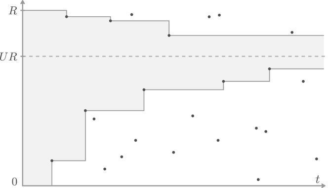
Figure 5: Illustration of the Poisson construction of $\mathbf{Q}^{1}_{R}$. Atoms of $P$ are represented with dark circles. At each time $t$, the vertical slice of the shaded region gives $I_{R}(t)$.

The following proposition shows that $(I_{P}(t);\,t\geq 0)$ corresponds to the distribution of $(I(t);\,t\geq 0)$, started from infinity.

Proposition 9.

Let $M$ be uniformly distributed on $[0,1]$ and independent of $P$. Then, for any $R\geq 0$, the process $(I_{R}(t);\,t\geq 0)$ defined as

$$\forall t\geq 0,\quad I_{R}(t)=MR+I_{P}(t)\cap[-MR,(1-M)R]$$

has distribution $\mathbf{Q}^{1}_{R}$. Moreover, for any $t$, $M$ is uniformly distributed on $I_{R}(t)$.

The proposition will follow from the next simple result.

Lemma 4.

Let $U$ and $V$ be independent uniform r.v. on $[0,1]$. Define the interval

$$I=\begin{cases}[0,U]&\text{if $V\leq U$},\\ [U,1]&\text{if $V>U$}\end{cases}$$

Then $|I|$ is independent of the event $\{V\leq U\}$, $|I|$ is a size-biased uniform r.v. on $[0,1]$, and $V$ is uniformly distributed on $I$.

Proof.

Let $A=\{V\leq U\}$ and $\bar{A}=\{V>U\}$. For any test function $\varphi$ and $\psi$, we can directly compute

$$\mathbb{P}(\varphi(V)\psi(|I|)\mathbf{1}_{A})=\int_{0}^{1}\int_{0}^{u}\varphi(v)\psi(u)\mathrm{d}v\mathrm{d}u=\mathbb{P}(A)\int_{0}^{1}2u\psi(u)\frac{1}{u}\int_{0}^{u}\varphi(v)\mathrm{d}v\mathrm{d}u$$

and

$$\mathbb{P}(\varphi(V)\psi(|I|)\mathbf{1}_{\bar{A}}) =\int_{0}^{1}\int_{u}^{1}\varphi(v)\psi(1-u)\mathrm{d}v\mathrm{d}u$$

$$=\mathbb{P}(\bar{A})\int_{0}^{1}2(1-u)\psi(1-u)\frac{1}{1-u}\int_{u}^{1}\varphi(v)\mathrm{d}v\mathrm{d}u.$$

∎

Proof of Proposition 9.

It is clear that $I_{R}(0)=[0,R]$. Let us consider the sequence of jumps times $(T_{i};\,i\geq 0)$ of $I_{R}$. By definition of the process, $T_{i+1}$ is the smallest time after $T_{i}$ such that there exists $X_{i+1}$ with $(T_{i+1},X_{i+1})\in P$ and $X_{i+1}\in I_{R}(T_{i})$. Then, if $I_{R}(T_{i})=[a,b]$,

$$I_{R}(T_{i+1})=[a,X_{i+1}]\mathbf{1}_{\{UR\leq X_{i+1}\}}+[X_{i+1},b]\mathbf{1}_{\{X_{i+1}<UR\}}$$

By the properties of homogeneous Poisson processes, $T_{i+1}-T_{i}$ is exponentially distributed with parameter $|I_{R}(T_{i})|$, and $X_{i+1}$ is uniformly distributed over $I_{R}(T_{i})$.

Using that $UR$ is uniformly distributed over $[0,R]$, a straightforward induction using Lemma 4 proves that for any $i$, $UR$ is uniformly distributed on $I_{R}(T_{i})$, and that $|I_{R}(T_{i+1})|$ is a size-biased r.v. uniform on $I_{R}(T_{i})$. This corresponds to the description of the transition mechanism of $(I(t);\,t\geq 0)$ under $\mathbf{Q}^{1}_{R}$ and proves the result. ∎

Define

$$\forall t\geq 0,\quad X(t)=|I(t)|,\quad X_{P}(t)=|I_{P}(t)|.$$

The coupling provided by the previous representation can be used to study the behavior of $(X(t);\,t\geq 0)$ as $R\to\infty$.

Corollary 2.

As $R\to\infty$, the process $(X(t);\,t\geq 0)$ under $\mathbf{Q}^{1}_{R}$ converges in distribution to $(X_{P}(t);\,t\geq 0)$ for the topology of uniform convergence on every set $[\varepsilon,\infty)$, $\varepsilon>0$. For any $t>0$, $X_{P}(t)$ follows a $\mathrm{Gamma}(2,t)$ distribution, that is

$$X_{P}(t)\sim t^{2}xe^{-tx}\mathrm{d}x.$$

Proof.

By the Poisson construction, if $X_{R}(t)\coloneqq|I_{R}(t)|$, then $(X_{R}(t);\,t\geq 0)$ is distributed as $(X(t);\,t\geq 0)$ under $\mathbf{Q}^{1}_{R}$. It is straightforward to see that for any $\varepsilon>0$, for large enough $R$ we have $X_{R}(t)=X_{P}(t)$ for any $t\geq\varepsilon$, proving the convergence part of the result.

By well-known properties of Poisson point processes, $P_{t}$ is a homogeneous Poisson point process with rate $t$. Moreover both the first positive and negative atom of $P_{t}$ follow an exponential distribution with parameter $t$, and are independent. This proves that $X_{P}(t)$ is gamma distributed with the right parameters. ∎

5.2 Self-similarity

From the transition mechanism of $(I(t);\,t\geq 0)$, we see that $(X(t);\,t\geq 0)$ is also a Markov process. Under $\mathbf{Q}^{1}_{R}$ it starts from $R$ and, conditional on $X(t)$, it jumps at rate $X(t)$ to $X(t)U^{*}$, where $U^{*}$ is a size-biased uniform r.v. on $[0,1]$. As the jump rate of $(X(t);\,t\geq 0)$ at time $t$ is $X(t)$, the process $(X(t);\,t\geq 0)$ is self-similar with index $-1$, in the sense that for any constant $c>0$, the following identity in law holds

$$(cX(ct);\,t\geq 0)\text{ under $\mathbf{Q}^{1}_{R}$ }\overset{(\mathrm{d})}{=}(X(t);\,t\geq 0)\text{ under $\mathbf{Q}^{1}_{cR}$}.$$

Positive Markov processes fulfilling the previous property are called positive self-similar Markov processes (pssMp), see [37] for an introductory exposition.

Remark 8.

In this work we will not make use of this connection with pssMp since all computations can be carried out directly from the Poisson construction. However this link could be used to generalize our results to a larger class of branching processes on the intervals, with more general fragmentation rules for the offspring distribution.

5.3 Convergence of the rescaled spine

Recall the definition of $F_{R}$ and $F_{R}^{-1}$ from (1). The following result provides the limit of the spine after rescaling time according to $F_{R}^{-1}$.

Proposition 10.

Let $0<u_{1}<\dots<u_{n}\leq 1$. Then

$$\big{(}F^{-1}_{R}(u_{1})X\circ F_{R}^{-1}(u_{1}),\dots,F^{-1}_{R}(u_{n})X\circ F_{R}^{-1}(u_{n})\big{)}\xrightarrow[\>R\to\infty\>]{\>\mathbf{Q}^{1}_{R}\>}(\gamma_{1},\cdots,\gamma_{n})$$

where the $\gamma_{i}$’s are independent Gamma r.v.’s with parameter $(2,1)$.

Proof.

We show the result by induction on $n$. Recall that $X(F^{-1}_{R}(u))$ has the same distribution as $Y_{1}\wedge RU+Y_{2}\wedge R(1-U)$ where $Y_{1}$, $Y_{2}$ are independent and exponentially distributed with mean $1/F^{-1}_{R}(u)$ and $U$ is uniform on $[0,1]$. For every $u\in(0,1]$, $1/F^{-1}_{R}(u)\sim R^{1-u}=o(R)$ so that $Y_{1}\wedge RU+Y_{2}\wedge R(1-U)=Y_{1}+Y_{2}$ with a probability going to $1$. This establishes the result at stage $1$.

Let us now assume that the property is satisfied at stage $n$. Conditional on the process $X$ up to time $F_{R}^{-1}(u_{n})$, the Markov property implies that the spine at $F^{-1}_{R}(u_{n+1})$ is distributed as $Y_{1}\wedge R_{n}U+Y_{2}\wedge R_{n}(1-U)$ where $R_{n}=X(F_{R}^{-1}(u_{n}))$, and $Y_{1}$, $Y_{2}$ are independent and exponentially distributed with mean $\big{(}F^{-1}_{R}(u_{n+1})-F^{-1}_{R}(u_{n})\big{)}^{-1}$. Since we have

$$\frac{1}{F^{-1}_{R}(u_{n+1})-F^{-1}_{R}(u_{n})}\sim\frac{1}{F^{-1}_{R}(u_{n+1})}=o\Big{(}\frac{1}{F^{-1}_{R}(u_{n})}\Big{)}=o(R_{n}),$$

as in the case $n=1$, this implies that $F^{-1}_{R}(X(u_{n+1}))$ is converging to an independent $\gamma_{n+1}$ random variable. ∎

6 The recombination $k$-spine tree

In the previous section we have characterized the large $N$, large $R$ behavior of the process giving the marks along a single spine. We now provide a similar characterization for the $k$-spine tree. We start with the following definition.

Definition 6.

Let us denote by $\mathbf{Q}^{k}_{I}$ the law of some r.v. $(I_{1},\dots,I_{k})$ and $(W_{1},\dots,W_{k-1})$ such that:

• $(W_{1},\dots,W_{k-1})$ are i.i.d. r.v.’s on $[0,1]$ with c.d.f. $F_{R}$;

• $I_{1}$ has distribution $\mathbf{Q}^{1}_{I}$ and is independent of $(W_{1},\dots,W_{k-1})$;

• $I_{i+1}=[I_{i};W_{i};I^{\prime}]$, where conditional on $(W_{1},\dots,W_{i})$ and $(I_{1},\dots,I_{i})$, $I^{\prime}$ has distribution $\mathbf{Q}^{1}_{I_{i}(W_{i})}$.

We also use the shorter notation $\mathbf{Q}^{k}_{R}$ for $\mathbf{Q}^{k}_{[0,R]}$.

6.1 Convergence of the tree

According to Proposition 10, it is natural to rescale time using $F_{R}$ as follows.

Definition 7.

We consider the rescaled $k$-spine measure as

$$\mathcal{Q}^{k}_{R}=\mathbf{Q}^{k}_{R}\circ F_{R}^{-1},$$

in the sense that under $\mathcal{Q}^{k}_{R}$

• The branch times are distributed as $(F_{R}(W_{1}),\dots,F_{R}(W_{k-1}))$;

• The spatial processes are distributed $(I_{1}\circ F_{R}^{-1},\dots,I_{k}\circ F_{R}^{-1})$;

where $(W_{1},\dots,W_{k-1})$ and $(I_{1},\dots,I_{k})$ are distributed respectively as the branch times and the spatial processes under $\mathbf{Q}^{k}_{R}$.

The following result is a straightforward extension of Proposition 10.

Proposition 11.

Under the rescaled $k$-spine measure $\mathcal{Q}_{R}^{k}$:

1. The branch times $(W_{1},\dots,W_{k-1})$ are distributed as i.i.d. uniform random variables on $[0,1]$.

2. Conditional on the $W_{i}$’s

   $$\Big{(}\big{(}F_{R}^{-1}(W_{1})X_{1}(W_{1}),\dots,F^{-1}_{R}(W_{k-1})X_{k-1}(W_{k-1})\big{)},\big{(}X_{1}(1),\dots,X_{k}(1)\big{)}\Big{)}\\ \xrightarrow[\>R\to\infty\>]{\>\mathcal{Q}_{R}^{k}\>}\big{(}(\gamma_{1},\dots,\gamma_{k-1}),(\bar{\gamma}_{1},\dots,\bar{\gamma}_{k})\big{)}$$

   where the $\gamma_{i}$’s and $\bar{\gamma}_{i}$’s are independent Gamma r.v.’s with parameter $(1,2)$.

Proof.

The proof goes along the same line the one of Proposition 10 and is left to the interested reader. ∎

6.2 Convergence of the chromosomic distance

In this section, we prove that the genealogical distance and the rescaled chromosomic distance coincide in the large $R$ limit under $\mathcal{Q}^{k}_{R}$. For $i<j$, set

$$W_{i,j}=W_{j,i}=\min\{W_{i},\dots,W_{j-1}\}$$

to be the time at which branches $i$ and $j$ split. Define

$$\forall i,j\leq k,\quad d(i,j)=1-W_{i,j},$$

which is the genealogical distance between the leaves of the $k$-spine tree.

Conditional on $(I_{1},\dots,I_{k})$ and $(W_{1},\dots,W_{k-1})$, let $M_{i}$ be uniformly distributed on $I_{i}(1)$. We define

$$\forall i,j\leq k,\quad D(i,j)=|M_{i}-M_{j}|$$

which is the chromosomic distance between the leaves. For later purpose, we also introduce the corresponding rescaled distance,

$$\forall i,j\leq k,\quad\bar{d}_{R}(i,j)=1-F_{R}(W_{i,j}),\quad\bar{D}_{R}(i,j)=\frac{\log D(i,j)\vee 2}{\log R}.$$ (16)

The next result provides an interesting relation between the genealogy of the branching process and the “geography” along the chromosome. Namely, on a logarithmic scale, the distance between two segments on the chromosome is directly related to the genealogy of the two segments.

Lemma 5.

We have

$$\forall i,j\leq k,\quad\frac{\log D(i,j)}{d(i,j)\log R}\xrightarrow[\>R\to\infty\>]{\>\mathcal{Q}_{R}^{k}\>}1.$$

Proof.

Let us work under $\mathbf{Q}^{k}_{R}$ and let $i<j$. By construction of the $k$-spine, conditional on $I_{i}(W_{i,j})$, $(I_{i}(t+W_{i,j});\,t\geq 0)$ and $(I_{j}(t+W_{i,j});\,t\geq 0)$ are independent and distributed as $\mathbf{Q}^{1}_{I_{i}(W_{i,j})}$. We know from the Poisson construction that, conditional on $I_{i}(W_{i,j})$, $M_{i}$ and $M_{j}$ are independent uniform variables on that interval. Therefore,

$$\frac{|M_{i}-M_{j}|}{X_{i}(W_{i,j})}$$

is a $\mathrm{Beta}(1,2)$ r.v. Write

$$\log D_{i,j}=\log|M_{i}-M_{j}|=\log\frac{|M_{i}-M_{j}|}{X_{i}(W_{i,j})}+\log W_{i,j}X_{i}(W_{i,j})-\log W_{i,j}.$$

From the previous point and Proposition 10,

$$\frac{1}{\log R}\log\frac{|M_{i}-M_{j}|}{X_{i}(W_{i,j})}+\frac{\log W_{i,j}X_{i}(W_{i,j})}{\log R}\xrightarrow[\>R\to\infty\>]{\>\mathbf{Q}^{k}_{R}\>}0.$$

Moreover

$$\frac{\log W_{i,j}}{\log R}=(F_{R}(W_{i,j})-1)(1+o_{R}(1))$$

so that

$$\frac{\log D_{i,j}}{(1-F_{R}(W_{i,j}))\log R}\xrightarrow[\>R\to\infty\>]{\>\mathbf{Q}^{k}_{R}\>}1.$$

The result follows by noting that the r.v. on the left-hand side has the same distribution under $\mathbf{Q}^{k}_{R}$ as

$$\frac{\log D_{i,j}}{d_{i,j}\log R}$$

under $\mathcal{Q}^{k}_{R}$. ∎

6.3 Proof of the main result

We can now proceed to the proof of our main result.

Proof of Theorem 2.

In order to ease the exposition, we only prove the result for $t=1$, but the proof is easily adapted for general $t>0$.

Recall that $\mathbf{Q}^{1,N}_{R}$ denotes the distribution of the $1$-spine provided in Definition 5. Let $\mathbf{Q}^{k,N}_{R}$ be the corresponding $k$-spine distribution, with i.i.d. branch times $(W_{1},\dots,W_{k-1})$ such that

$$W_{i}\overset{\mathrm{(d)}}{=}\lfloor WN\rfloor,\qquad\forall u\leq 1,\quad\mathbb{P}(W\leq u)=F_{R}(u).$$ (17)

for the function $F_{R}$ defined in (1).

Set

$$\forall i,j\leq k,\quad\bar{d}^{N}_{R}(i,j)=1-F_{R}(W^{N}_{i,j}),\quad\bar{D}^{N}_{R}(i,j)=\frac{\log|M_{i}-M_{j}|\vee 2}{\log R},$$

where the $M_{i}$ are uniformly distributed on the $I_{i}(N)$. In order to use Theorem 6, we need to compute the limit of

$$\mathbf{Q}^{k,N}_{R}\Big{[}\Delta_{k}\cdot\varphi\big{(}\bar{d}^{N}_{R}(i,j),\bar{D}^{N}_{R}(i,j),X^{N}_{i}(1);\,i,j\leq k\big{)}\Big{]}$$

where for the branching process with recombination,

$$\Delta_{k}=\prod_{u\in S}\frac{1}{d_{u}!}\prod_{i=1}^{k-1}\frac{X_{i}^{N}(W^{N}_{i})}{\delta_{N}F_{R}(W_{i}^{N})}\prod_{i=1}^{k}\frac{1}{X^{N}_{i}(1)}$$

with

$$\forall x\geq 0,\quad\delta_{N}F_{R}(x)=N\big{(}{F_{R}(x+\tfrac{1}{N})-F_{R}(x)}\big{)}.$$

According to Proposition 8, under $\mathbf{Q}^{1,N}_{R}$ the process $I^{N}$ converges to the limiting process with distribution $\mathbf{Q}^{1}_{R}$ introduced in Definition 5. Therefore, Proposition 7 proves that

$$\big{(}(I^{N}_{1},\dots,I^{N}_{k}),(W^{N}_{1},\dots,W^{N}_{k-1})\big{)}\xrightarrow[\>N\to\infty\>]{\>\mathbf{Q}^{k,N}_{R}\>}\big{(}(I_{1},\dots,I_{k}),(W_{1},\dots,W_{k-1})\big{)}$$

where the limiting variables have distribution $\mathbf{Q}^{k}_{R}$. Since the variables $(W_{1},\dots,W_{k-1})$ are a.s. distinct under $\mathbf{Q}^{k}_{R}$, it entails that

$$\prod_{u\in S}\frac{1}{d_{u}!}\xrightarrow[\>N\to\infty\>]{\>\mathbf{Q}^{k,N}_{R}\>}\frac{1}{2^{k-1}}.$$

Corollary 3 provides enough uniform integrability to conclude that

$$\lim_{N\to\infty} \mathbf{Q}^{k,N}_{R}\Big{[}\prod_{u\in S}\frac{1}{d_{u}!}\prod_{i=1}^{k-1}\frac{X_{i}^{N}(W^{N}_{i})}{\delta_{N}F_{R}(W_{i}^{N})}\prod_{i=1}^{k}\frac{1}{X^{N}_{i}(1)}\cdot\varphi\big{(}\bar{d}^{N}_{R}(i,j),\bar{D}^{N}_{R}(i,j),X^{N}_{i}(1);\,i,j\leq k\big{)}\Big{]}$$

$$=\frac{1}{2^{k-1}}\mathbf{Q}^{k}_{R}\Big{[}\prod_{i=1}^{k-1}\frac{X_{i}(W_{i})}{F_{R}^{\prime}(W_{i})}\prod_{i=1}^{k}\frac{1}{X_{i}(1)}\cdot\varphi\big{(}\bar{d}_{R}(i,j),\bar{D}_{R}(i,j),X_{i}(1);\,i,j\leq k\big{)}\Big{]}$$

$$=\frac{1}{2^{k-1}}{\cal Q}^{k}_{R}\Big{[}\prod_{i=1}^{k-1}X_{i}(W_{i})(F^{-1}_{R})^{\prime}(W_{i})\prod_{i=1}^{k}\frac{1}{X_{i}(1)}\cdot\varphi\big{(}d(i,j),\bar{D}_{R}(i,j),X_{i}(1);\,i,j\leq k\big{)}\Big{]}$$

where the last line follows by rescaling time according to (1) and the distances are defined in (16). The first observation is that, a.s.,

$$\frac{1}{\log R}\frac{(F_{R}^{-1})^{\prime}(W_{i})}{F_{R}^{-1}(W_{i})}=\frac{R^{W_{i}}}{R^{W_{i}}-1}\longrightarrow 1.$$

The second observation is that conditional on $(W_{1},\dots,W_{k-1})$, according to Proposition 11,

$$\big{(}(F^{-1}_{R}(W_{i})X_{i}(W_{i});\,i\leq k-1),(X_{i}(1);\,i\leq k)\big{)}\xrightarrow[\>R\to\infty\>]{\>\mathcal{Q}^{k}_{R}\>}\big{(}(\gamma_{1},\dots,\gamma_{k-1}),(\bar{\gamma}_{1},\dots,\bar{\gamma}_{k})\big{)}$$

where the limiting r.v. are $\mathrm{Gamma}(2,1)$ distributed and independent. Let $\beta\in(1,2)$ and define

$$\forall u\in[0,1],\quad\Phi(u)=\frac{1}{\log R\,F_{R}^{\prime}(u)}=u+\frac{1}{R-1}$$

By reverting the previous change of variable

$$\mathcal{Q}^{k}_{R}\Big{[}\prod_{i=1}^{k-1}\Big{(}\frac{(F^{-1}_{R})^{\prime}(W_{i})X_{i}(W_{i})}{\log R}\Big{)}^{\beta}\prod_{i=1}^{k}\frac{1}{X_{i}(1)^{\beta}}\Big{]}=\mathbf{Q}^{k}_{R}\Big{[}\prod_{i=1}^{k-1}\big{(}X_{i}(W_{i})\Phi(W_{i})\big{)}^{\beta}\prod_{i=1}^{k}\frac{1}{X_{i}(1)^{\beta}}\Big{]}.$$

By Corollary 3, the r.h.s. is uniformly bounded in $R$. This provides enough uniform integrability to get

$$\lim_{R\to\infty}\Big{(}\frac{1}{2\log R}\Big{)}^{k-1}\mathcal{Q}^{k}_{R}\Big{[} \prod_{i=1}^{k-1}X_{i}(W_{i})(F_{R}^{-1})^{\prime}(W_{i})\prod_{i=1}^{k}\frac{1}{X_{i}(1)}\cdot\varphi\big{(}d(i,j),\bar{D}_{R}(i,j),X_{i}(1);\,i,j\leq k\big{)}\Big{]}$$

$$=\mathbb{E}\Big{[}\prod_{i=1}^{k}\frac{1}{\gamma_{i}}\cdot\varphi\big{(}1-W_{i,j},1-W_{i,j},\gamma_{i};\,i,j\leq k\big{)}\Big{]}$$

$$=\mathbb{E}\Big{[}\varphi\big{(}1-W_{i,j},1-W_{i,j},Y_{i};\,i,j\leq k\big{)}\Big{]}$$

where $\gamma_{i}$ are i.i.d. $\mathrm{Gamma}(2,1)$ r.v., $Y_{i}$ are i.i.d. standard exponential random variable, and we have used Lemma 5 for the convergence of the distances.

We can now apply Theorem 6 with

$$\alpha_{N}=\frac{1}{N\log R},\qquad\beta_{N}(x)=x,\qquad\gamma_{N}(t)=1-F_{R}\big{(}1-\tfrac{t}{N}\big{)}.$$

Recall that $Z_{N}$ denotes the population size and that from Proposition 1

$$\lim_{N\to\infty}N\mathbf{P}_{R}(Z_{N}>0)$$

exists and that

$$\lim_{R\to\infty}\lim_{N\to\infty}\frac{N\log R}{R}\mathbf{P}_{R}(Z_{N}>0)=1.$$

Therefore,

$$\lim_{N\to\infty}\frac{k!N^{k-1}R}{(N\log R)^{k}\mathbf{P}_{R}(Z_{N}>0)}\mathbf{Q}^{k,N}_{R}\Big{[}\Delta_{k}\cdot\varphi\big{(}\bar{d}^{N}_{R}(i,j),\bar{D}^{N}_{R}(i,j),X_{i}^{N}(1);\,i,j\leq k\big{)}\Big{]}$$

exists and we have

$$\lim_{R\to\infty} \lim_{N\to\infty}\frac{k!N^{k-1}R}{(N\log R)^{k}\mathbf{P}_{R}(|T_{N}|>0)}\mathbf{Q}^{k,N}_{R}\Big{[}\Delta_{k}\cdot\varphi\big{(}\bar{d}^{N}_{R}(i,j),\bar{D}^{N}_{R}(i,j),X_{i}^{N}(1);\,i,j\leq k\big{)}\Big{]}$$

$$=\lim_{R\to\infty}\lim_{N\to\infty}\frac{k!}{(\log R)^{k-1}}\mathbf{Q}^{k,N}_{R}\Big{[}\Delta_{k}\cdot\varphi\big{(}\bar{d}^{N}_{R}(i,j),\bar{D}^{N}_{R}(i,j),X_{i}^{N}(1);\,i,j\leq k\big{)}\Big{]}$$

$$=k!\,\mathbb{E}\Big{[}\varphi\big{(}1-W_{i,j},1-W_{i,j},Y_{i};\,i,j\leq k\big{)}\Big{]}$$

Applying Theorem 6 for the large $N$ limit, then Proposition 3 for the large $R$ limit, and finally Proposition 5 and Proposition 4 for the polynomials of the Brownian CPP with independent marks proves the result. Note that since the total mass of the Brownian CPP is exponentially distributed, it fulfills the moment condition (7). For the large $N$ limit, the size of the branching process with recombination is stochastically dominated by a Galton–Watson process with $\mathrm{Poisson}(1+R/N)$ offspring distribution. The size of this process, conditional on survival at time $N$ and rescaled by $N$, is well-known to converge to an exponential distribution, see for instance [35, Theorem 2.1]. This readily shows that (12) is also fulfilled by the large $N$ limit, for each fixed $R$. ∎

Remark 9.

In the above proof we have made use of Theorem 4 to identify the large $N$ limit of the genealogy. It is possible to prove the result without relying on our extension of the Gromov-weak topology by constructing the branching process with recombination by superimposing on a Galton–Watson tree with $\mathrm{Poisson}(1+R/N)$ offspring distribution a process along the branches describing the recombination events as in [3]. The large $N$ limit could then be expressed by means of the superprocess limit associated to that branching model.

Acknowledgements.

We greatly thank Amaury Lambert for initiating this project, for very helpful discussions, and for his interest in this work.

Appendix A Appendix

A.1 Continuity of the concatenation map

For two càdlàg functions $x$ and $y$ and a positive real $r$, recall that

$$[x;r;y]\colon t\mapsto\begin{cases}x(t)&\text{if $t<r$}\\ y(t-r)&\text{if $t\geq r$}\end{cases}$$

denotes the concatenation of $x$ and $y$ at time $r$.

Lemma 6.

Suppose that we have two sequences of càdlàg functions $(x_{n})$ and $(y_{n})$ that converge to $x$ and $y$ respectively in the Skorohod topology. Moreover, suppose that $(r_{n})$ converges to $r>0$, and that $x$ is continuous at $r$. Then

$$[x_{n};r_{n};y_{n}]\longrightarrow[x;r;y].$$

Proof.

Recall that a sequence $(z_{n})$ converges to some $z$ in the Skorohod topology if ​f for each $T\geq 0$, we can find a sequence of continuous increasing maps $\lambda_{n}$ such that

$$\lim_{n\to\infty}\sup_{t\leq T}|\lambda_{n}(t)-t|=0$$ (18)

and

$$\lim_{n\to\infty}\sup_{t\leq T}|z_{n}\circ\lambda_{n}(t)-z(t)|=0,$$ (19)

see for instance [15, Proposition 5.3].

Fix $T>r$, and let $(\lambda_{n})$ and $(\mu_{n})$ fulfill (18) and $\eqref{eq:sk2}$ with $(z_{n})$ replaced by $(x_{n})$ and $(y_{n})$ respectively. For $\varepsilon>0$, let $\delta$ be such that

$$|t-r|<\delta\implies|x(t)-x(r)|<\varepsilon.$$

Using that

$$\lambda_{n}(r-\delta)\to r-\delta,\quad\lambda_{n}(r+\delta)\to r+\delta,\quad r_{n}\to r$$

we know that for $n$ large enough $\lambda_{n}(r-\delta)<r_{n}<\lambda_{n}(r+\delta)$. Define

$$\forall t\geq 0,\quad\lambda^{\prime}_{n}(t)=\begin{dcases}\lambda_{n}(t)&\text{if $t\leq r-\delta$}\\ \lambda_{n}(r-\delta)+\big{(}t-(r-\delta)\big{)}\frac{r_{n}-\lambda_{n}(r-\delta)}{\delta}&\text{if $r-\delta<t\leq r$}\\ \lambda_{n}(r+\delta)+\big{(}t-(r+\delta)\big{)}\frac{\lambda_{n}(r+\delta)-r_{n}}{\delta}&\text{if $r<t\leq r+\delta$}\\ \lambda_{n}(t)&\text{if $t\geq r+\delta$}\end{dcases}$$

which is continuous, increasing, and is designed so that $\lambda^{\prime}_{n}(r)=r_{n}$ and coincides with $\lambda_{n}$ outside of $(r-\delta,r+\delta)$. Now,

$$\sup_{(r-\delta,r+\delta)}|x_{n}\circ\lambda^{\prime}_{n}(t)-x(t)| \leq\sup_{(r-\delta,r+\delta)}|x_{n}\circ\lambda^{\prime}_{n}(t)-x(r)|+\sup_{(r-\delta,r+\delta)}|x(r)-x(t)|$$

$$\leq\sup_{(r-\delta,r+\delta)}|x_{n}\circ\lambda_{n}(t)-x(r)|+\varepsilon$$

$$\leq\sup_{(r-\delta,r+\delta)}|x_{n}\circ\lambda_{n}(t)-x(t)|+2\varepsilon.$$

Therefore, up to modifying $\lambda_{n}$ in this way and extracting a subsequence, we can always assume that, in addition to (18) and (19), we have $\lambda_{n}(r)=r_{n}$.

Let us now denote

$$z_{n}=[x_{n};r_{n};y_{n}],\quad z=[x;r;y]$$

and define

$$\forall t\geq 0,\quad\nu_{n}(t)=\begin{cases}\lambda_{n}(t)&\text{if $t<r$}\\ \mu_{n}(t-r)+r_{n}&\text{if $t\geq r$}\end{cases}$$

to be the concatenation of the two increasing maps. Clearly $(\nu_{n})$ fulfills (18), and using that $\nu_{n}(t)<r_{n}$ if ​f $t<r$, we obtain

$$z_{n}\circ\nu_{n}(t)=\begin{cases}x_{n}\circ\lambda_{n}(t)&\text{if $t<r$}\\ y_{n}\circ\mu_{n}(t-r)&\text{if $t\geq r$}\end{cases}$$

from which it follows that

$$\sup_{t\leq T}|z_{n}\circ\nu_{n}(t)-z(t)|\leq\sup_{t\leq T}|x_{n}\circ\lambda_{n}(t)-x(t)|+\sup_{t\leq T}|y_{n}\circ\mu_{n}(t)-y(t)|$$

proving the result. ∎

A.2 Uniform integrability results

The aim of this technical section is to prove the uniform integrability of the inverse of the $k$-spine.

Lemma 7.

For any $\alpha<1$ and $t>0$, there exists a constant $C$ such that

$$\forall R>0,\,s\leq t,\quad\mathbf{Q}^{1}_{R}\Big{[}\frac{1}{X(s)^{1+\alpha}}\Big{]}\leq C\Big{(}\frac{1}{R^{1+\alpha}}+1\Big{)}.$$

There also exists a constant $C^{\prime}$ such that for $N$ sufficiently large

$$\forall R>0,\,s\leq t,\quad\mathbf{Q}^{1,N}_{R}\Big{[}\frac{1}{X^{N}(s)^{1+\alpha}}\Big{]}\leq C^{\prime}\Big{(}\frac{1}{R^{1+\alpha}}+1\Big{)}.$$

Proof.

As $X^{N}$ and $X$ are non-increasing, we have

$$\mathbf{Q}^{1}_{R}\Big{[}\frac{1}{X(s)^{1+\alpha}}\Big{]}\leq\mathbf{Q}^{1}_{R}\Big{[}\frac{1}{X(t)^{1+\alpha}}\Big{]}$$

and

$$\mathbf{Q}^{1,N}_{R}\Big{[}\frac{1}{X^{N}(s)^{1+\alpha}}\Big{]}\leq\mathbf{Q}^{1,N}_{R}\Big{[}\frac{1}{X^{N}(t)^{1+\alpha}}\Big{]}.$$

It is a direct consequence of the Poisson construction that $X(t)$ under $\mathbf{Q}^{1}_{R}$ is stochastically dominated by $X(t)$ under $\mathbf{Q}^{1}_{R^{\prime}}$ if $R\leq R^{\prime}$. Therefore

$$\forall R\geq 1,\quad\mathbf{Q}^{1}_{R}\Big{[}\frac{1}{X(t)^{1+\alpha}}\Big{]}\leq\mathbf{Q}^{1}_{1}\Big{[}\frac{1}{X(t)^{1+\alpha}}\Big{]}.$$

Moreover, by self-similarity,

$$\forall R\leq 1,\quad\mathbf{Q}^{1}_{R}\Big{[}\frac{1}{X(t)^{1+\alpha}}\Big{]}=\frac{1}{R^{1+\alpha}}\mathbf{Q}^{1}_{1}\Big{[}\frac{1}{X(Rt)^{1+\alpha}}\Big{]}\leq\frac{1}{R^{1+\alpha}}\mathbf{Q}^{1}_{1}\Big{[}\frac{1}{X(t)^{1+\alpha}}\Big{]}.$$

Together, these two identities yields that

$$\forall R>0,\quad\mathbf{Q}^{1}_{R}\Big{[}\frac{1}{X(t)^{1+\alpha}}\Big{]}\leq\mathbf{Q}^{1}_{1}\Big{[}\frac{1}{X(t)^{1+\alpha}}\Big{]}\Big{(}\frac{1}{R^{1+\alpha}}+1\Big{)}.$$

The first part of the result is proved provided that

$$\mathbf{Q}^{1}_{1}\Big{[}\frac{1}{X(t)^{1+\alpha}}\Big{]}<\infty.$$

Recalling that $X(t)$ has the same distribution as $Y_{1}\wedge U+Y_{2}\wedge(1-U)$ where $Y_{1}$ and $Y_{2}$ are exponentially distributed with mean $1/t$ and $U$ uniformly distributed on $[0,1]$, a direct computation shows that

$$\mathbf{Q}^{1}_{1}\Big{[}\frac{1}{X(t)^{1+\alpha}}\Big{]}\leq\mathbb{E}\Big{[}\Big{(}\frac{1}{Y_{1}+Y_{2}}\Big{)}^{1+\alpha}\Big{]}+2\mathbb{E}\Big{[}\Big{(}\frac{1}{Y_{1}+U}\Big{)}^{1+\alpha}\Big{]}+1<\infty.$$

The second part of the result follows from the fact that, for any $c>1$, for large enough $N$,

$$\forall R>0,\quad X^{N}(t)\text{ under $\mathbf{Q}^{1,N}_{R}$}\quad\overset{\mathrm{(d)}}{\geq}\quad X(ct)\text{ under $\mathbf{Q}^{1}_{R}$}.$$

To see this note that $X^{N}$ and $X$ visit the same sequence of states in distribution. Thus stochastic domination follows if $(X(ct);\,t\geq 0)$ jumps faster than $(X^{N}(t);\,t\geq 0)$. Started from $\rho$, the process $X^{N}$ jumps after a time $T^{N}/N$ whereas $X$ jumps after a time $T$ with

$$T^{N}\sim\mathrm{Geometric}\Big{(}\frac{\rho}{N}\Big{)},\qquad T_{\rho}\sim\mathrm{Exponential}(\rho).$$

A direct computation shows that, provided $1-\exp(-c\rho/N)\leq\rho/N$, $T/c$ is stochastically dominated by $T^{N}/N$. The latter condition clearly holds for all $\rho\leq R$ for large enough $N$. ∎

We now apply the previous estimate inductively to the $k$-spine, first to be able to take the large $N$ limit, then to take the large $R$ limit. Recall the notation $X^{N}_{i}$ for the rescaled marks along branch $i$ and the notation $W^{N}_{i}$ for the rescaled $i$-th branch time, and the notation

$$\forall u\in[0,1],\quad\Phi(u)=u+\frac{1}{R-1}.$$

Corollary 3.

For any $R>1,k\geq 1$, and $\beta\in(1,2)$,

$$\sup_{R>1}\mathbf{Q}^{k}_{R}\Big{[}\prod_{i=1}^{k-1}(\Phi(W_{i})X_{i}(W_{i}))^{\beta}\prod_{i=1}^{k}\Big{(}\frac{1}{X_{i}(1)}\Big{)}^{\beta}\Big{]}<\infty.$$

Further,

$$\sup_{N>1}\mathbf{Q}^{k,N}_{R}\Big{[}\prod_{i=1}^{k-1}\Big{(}\frac{X_{i}(W^{N}_{i})}{\delta_{N}F_{R}(W_{i}^{N})}\Big{)}^{\beta}\prod_{i=1}^{k}\frac{1}{X^{N}_{i}(1)^{\beta}}\Big{]}<\infty.$$

Proof.

We only prove the result in the continuum setting. The discrete case can be proved along the same lines. Applying the Markov property to $X_{k+1}$ at time $W_{k}$ and using Lemma 7 yields

$$\mathbf{Q}^{k+1}_{R}\Big{[} \prod_{i=1}^{k}\big{(}\Phi(W_{i})X_{i}(W_{i})\big{)}^{\beta}\prod_{i=1}^{k+1}\Big{(}\frac{1}{X_{i}(1)}\Big{)}^{\beta}\Big{]}$$

$$=\mathbf{Q}^{k+1}_{R}\Big{[}\prod_{i=1}^{k}\big{(}\Phi(W_{i})X_{i}(W_{i})\big{)}^{\beta}\prod_{i=1}^{k}\frac{1}{X_{i}(1)^{\beta}}\mathbf{Q}_{X_{k}(W_{k})}^{1}\Big{[}\frac{1}{X(1-{W_{k}})^{\beta}}\Big{]}\Big{]}$$

$$\leq\mathbf{Q}^{k+1}_{R}\Big{[}\prod_{i=1}^{k}\big{(}\Phi(W_{i})X_{i}(W_{i})\big{)}^{\beta}\prod_{i=1}^{k}\frac{1}{X_{i}(1)^{\beta}}C\Big{(}\frac{1}{X_{k}(W_{k})^{\beta}}+1\Big{)}\Big{]}$$

$$\leq\begin{multlined}2^{\beta}C\mathbf{Q}^{k}_{R}\Big{[}\prod_{i=1}^{k-1}\big{(}\Phi(W_{i})X_{i}(W_{i})\big{)}^{\beta}\prod_{i=1}^{k}\frac{1}{X_{i}(1)^{\beta}}\Big{]}\\ +C\mathbf{Q}^{k}_{R}\Big{[}\big{(}\Phi(W_{k})X_{k}(W_{k})\big{)}^{\beta}\prod_{i=1}^{k-1}\big{(}\Phi(W_{i})X_{i}(W_{i})\big{)}^{\beta}\prod_{i=1}^{k}\frac{1}{X_{i}(1)^{\beta}}\Big{]}\end{multlined}2^{\beta}C\mathbf{Q}^{k}_{R}\Big{[}\prod_{i=1}^{k-1}\big{(}\Phi(W_{i})X_{i}(W_{i})\big{)}^{\beta}\prod_{i=1}^{k}\frac{1}{X_{i}(1)^{\beta}}\Big{]}\\ +C\mathbf{Q}^{k}_{R}\Big{[}\big{(}\Phi(W_{k})X_{k}(W_{k})\big{)}^{\beta}\prod_{i=1}^{k-1}\big{(}\Phi(W_{i})X_{i}(W_{i})\big{)}^{\beta}\prod_{i=1}^{k}\frac{1}{X_{i}(1)^{\beta}}\Big{]}$$

where in the last inequality, we used the fact that $\Phi(u)\leq 2$ for every $u\in[0,1]$. Let $p,q\geq 0$ such that $\frac{1}{p}+\frac{1}{q}=1$ and take $q$ close enough to $1$ such that $q\beta\in(1,2)$. By Hölder’s inequality, the second term on the r.h.s. is bounded from above by

$$\bigg{(}\mathbf{Q}^{k}_{R}\Big{[}\prod_{i=1}^{k-1}\big{(}\Phi(W_{i})X_{i}(W_{i})\big{)}^{q\beta}\prod_{i=1}^{k}\frac{1}{X_{i}(1)^{q\beta}}\Big{]}\bigg{)}^{1/q}\bigg{(}\mathbf{Q}^{k}_{R}\Big{[}\big{(}\Phi(W_{1})X_{1}(W_{1})\big{)}^{p\beta}\big{]}\bigg{)}^{1/p}$$

Further,

$$\mathbf{Q}^{k}_{R}\Big{[}\big{(}\Phi(W_{1})X_{1}(W_{1})\big{)}^{p\beta}\big{]} \leq 2^{p\beta-1}\mathbf{Q}^{k}_{R}\Big{[}\big{(}W_{1}X_{1}(W_{1})\big{)}^{p\beta}\Big{]}+2^{p\beta-1}\mathbf{Q}^{k}_{R}\Big{[}\Big{(}\frac{X_{1}(W_{1})}{R-1}\Big{)}^{p\beta}\Big{]}$$

$$\leq 2^{p\beta-1}\mathbf{Q}^{k}_{\infty}\Big{[}\big{(}W_{1}X_{1}(W_{1})\big{)}^{p\beta}\Big{]}+2^{p\beta-1}\Big{(}\frac{R}{R-1}\Big{)}^{p\beta}$$

Finally, $W_{1}X_{1}(W_{1})$ is a $\mathrm{Gamma}(2,1)$ r.v. under $\mathbf{Q}^{k}_{\infty}$. The result follows by a straightforward induction since the case $k=1$ was proved in Lemma 7. ∎

References

- [1] Krishna B. Athreya and Peter E. Ney. Branching Processes. Grundlehren der mathematischen Wissenschaften. Springer-Verlag Berlin Heidelberg, 1972.
- [2] Ellen Baake and Inke Herms. Single-crossover dynamics: Finite versus infinite populations. Bulletin of Mathematical Biology, 70:603–624, 2008.
- [3] Stuart J. E. Baird, Nicholas H. Barton, and Alison M. Etheridge. The distribution of surviving blocks of an ancestral genome. Theoretical Population Biology, 64:451–471, 2003.
- [4] Vincent Bansaye, Jean-François Delmas, Laurence Marsalle, and Viet Chi Tran. Limit theorems for Markov processes indexed by continuous time Galton-Watson trees. The Annals of Applied Probability, 21:2263–2314, 2011.
- [5] Jean Bertoin and Maria-Emilia Caballero. Entrance from for increasing semi-stable Markov processes. Bernoulli, 8:195–205, 2002.
- [6] Jean Bertoin and Marc Yor. The entrance laws of self-similar Markov processes and exponential functionals of lévy processes. Potential Analysis, 17:389–400, 2002.
- [7] John D Biggins and Andreas E. Kyprianou. Measure change in multitype branching. Advances in Applied Probability, 36:544–581, 2004.
- [8] Donald A. Dawson. Measure-Valued Markov Processes. Lecture Notes in Mathematics. Springer, Berlin, Heidelberg, 1993.
- [9] Andrej Depperschmidt and Andreas Greven. Tree-valued Feller diffusion. arXiv 1904.02044, 2019.
- [10] Andrej Depperschmidt, Andreas Greven, and Peter Pfaffelhuber. Marked metric measure spaces. Electronic Communications in Probability, 16:174–188, 2011.
- [11] Jean-Jil Duchamps and Amaury Lambert. Mutations on a random binary tree with measured boundary. The Annals of Applied Probability, 28:2141–2187, 2018.
- [12] Thomas Duquesne and Jean-François Le Gall. Random Trees, Lévy Processes and Spatial Branching Processes. Astérisque, 2002.
- [13] Richard Durrett. Probability Models for DNA Sequence Evolution. Probability and its Applications. Springer, New York, NY, second edition, 2008.
- [14] Richard Durrett. Probability: Theory and Examples. Cambridge Series in Statistical and Probabilistic Mathematics. Cambridge University Press, fifth edition, 2019.
- [15] Stewart N. Ethier and Thomas G. Kurtz. Markov Processes: Characterization and Convergence. Wiley Series in Probability and Statistics. John Wiley & Sons, Inc., 1986.
- [16] Ronald A. Fisher. A fuller theory of “junctions” in inbreeding. Heredity, 8:187–197, 1954.
- [17] Félix Foutel-Rodier, Amaury Lambert, and Emmanuel Schertzer. Exchangeable coalescents, ultrametric spaces, nested interval-partitions: A unifying approach. The Annals of Applied Probability, 31:2046–2090, 2021.
- [18] Andreas Greven, Peter Pfaffelhuber, and Anita Winter. Convergence in distribution of random metric measure spaces (-coalescent measure trees). Probability Theory and Related Fields, 145:285–322, 2009.
- [19] Robert C. Griffiths and Paul Marjoram. An ancestral recombination graph. In Progress in population genetics and human evolution, pages 257–270. Springer, 1997.
- [20] Stephan Gufler. A representation for exchangeable coalescent trees and generalized tree-valued Fleming-Viot processes. Electronic Journal of Probability, 23:42 pp., 2018.
- [21] Simon C. Harris, Samuel G. G. Johnston, and Matthew I. Roberts. The coalescent structure of continuous-time Galton–Watson trees. The Annals of Applied Probability, 30:1368–1414, 2020.
- [22] Simon C. Harris and Matthew I. Roberts. The many-to-few lemma and multiple spines. Annales de l’Institut Henri Poincaré, Probabilités et Statistiques, 53:226–242, 2017.
- [23] Thijs Janzen and Verónica Miró Pina. Estimating the time since admixture from phased and unphased molecular data. Molecular Ecology Resources, 2021.
- [24] Samuel G. G. Johnston. The genealogy of Galton-Watson trees. Electronic Journal of Probability, 24:35 pp., 2019.
- [25] Olav Kallenberg. Foundations of Modern Probability. Probability and its Applications. Springer-Verlag New York, second edition, 2002.
- [26] John F. C. Kingman. The representation of partition structures. Journal of the London Mathematical Society, 18:374–380, 1978.
- [27] Amaury Lambert. The contour of splitting trees is a Lévy process. The Annals of Probability, 38:348–395, 2010.
- [28] Amaury Lambert, Verónica Miró Pina, and Emmanuel Schertzer. Chromosome painting: How recombination mixes ancestral colors. The Annals of Applied Probability, 31:826–864, 2021.
- [29] Amaury Lambert and Lea Popovic. The coalescent point process of branching trees. The Annals of Applied Probability, 23:99–144, 2013.
- [30] Jean-François Le Gall. Brownian excursions, trees and measure-valued branching processes. The Annals of Probability, 19:1399–1439, 1991.
- [31] Russell Lyons, Robin Pemantle, and Yuval Peres. Conceptual proofs of criteria for mean behavior of branching processes. The Annals of Probability, 23:1125–1138, 1995.
- [32] Paul Marjoram and Jeff D. Wall. Fast “coalescent” simulation. BMC Genetics, 7:16, 2006.
- [33] Gilean A. T. McVean and Niall J. Cardin. Approximating the coalescent with recombination. Philosophical Transactions of the Royal Society B: Biological Sciences, 360:1387–1393, 2005.
- [34] Martin Möhle and Serik Sagitov. A classification of coalescent processes for haploid exchangeable population models. The Annals of Probability, 29:1547–1562, 2001.
- [35] Neil O’Connell. The genealogy of branching processes and the age of our most recent common ancestor. Advances in Applied Probability, 27:418–442, 1995.
- [36] Tomoko Ohta and Motoo Kimura. Linkage disequilibrium due to random genetic drift. Genetical Research, 13:47–55, 1969.
- [37] Juan Carlos Pardo and Víctor Rivero. Self-similar Markov processes. Boletín de la Sociedad Matemática Mexicana: Tercera Serie, 19:201–235, 2013.
- [38] Jim Pitman. Coalescents with multiple collisions. The Annals of Probability, 27:1870–1902, 1999.
- [39] Lea Popovic. Asymptotic genealogy of a critical branching process. The Annals of Applied Probability, 14:2120–2148, 2004.
- [40] Lea Popovic and Mariolys Rivas. The coalescent point process of multi-type branching trees. Stochastic Processes and their Applications, 124:4120–4148, 2014.
- [41] Yan-Xia Ren, Renming Song, and Zhenyao Sun. A 2-spine decomposition of the critical Galton-Watson tree and a probabilistic proof of Yaglom’s theorem. Electronic Communications in Probability, 23:1–12, 2018.
- [42] Serik Sagitov. The general coalescent with asynchronous mergers of ancestral lines. Journal of Applied Probability, 36:1116–1125, 1999.
- [43] Jason Schweinsberg. Coalescent processes obtained from supercritical Galton–Watson processes. Stochastic Processes and their Applications, 106:107–139, 2003.
- [44] Zhan Shi. Branching Random walks, volume 2151 of Lecture Notes in Mathematics. Springer, Cham, 2015.