Bounding Training Data Reconstruction in Private (Deep) Learning

Abstract

Differential privacy is widely accepted as the de facto method for preventing data leakage in ML, and conventional wisdom suggests that it offers strong protection against privacy attacks. However, existing semantic guarantees for DP focus on membership inference, which may overestimate the adversary’s capabilities and is not applicable when membership status itself is non-sensitive. In this paper, we derive semantic guarantees for DP mechanisms against training data reconstruction attacks under a formal threat model. We show that two distinct privacy accounting methods—Rényi differential privacy and Fisher information leakage—both offer strong semantic protection against data reconstruction attacks.

1 Introduction

Machine learning models are known to memorize their training data. This vulnerability can be exploited by an adversary to compromise the privacy of participants in the training dataset when given access to the trained model and/or its prediction interface (Fredrikson et al., 2014, 2015; Shokri et al., 2017; Carlini et al., 2019). By far the most accepted mitigation measure against such privacy leakage is differential privacy (DP; Dwork et al. (2014)), which upper bounds the information contained in the learner’s output about its training data via statistical divergences. However, such a differential guarantee is often hard to interpret, and it is unclear how much privacy leakage can be tolerated for a particular application (Jayaraman & Evans, 2019).

Recent studies have derived semantic guarantees for differential privacy, that is, how does the private mechanism limit an attacker’s ability to extract private information from the trained model? For example, Yeom et al. (2018) showed that a differentially private learner can reduce the success rate of a membership inference attack to close to that of a random coin flip. Semantic guarantees serve as more interpretable translations of the DP guarantee and provide reassurance of protection against privacy attacks. However, existing semantic guarantees focus on protection of membership status, which has several limitations: 1. There are many scenarios where membership status itself is not sensitive but the actual data value is, e.g., census data and location data. 2. It only bounds the leakage of the binary value of membership status as opposed to how much information can be extracted. 3. Membership inference is empirically much easier than powerful attacks such as training data reconstruction (Carlini et al., 2019; Zhang et al., 2020; Balle et al., 2022), and hence it may be possible to provide a strong semantic guarantee against data reconstruction attacks even when membership status cannot be protected.

In this work, we focus on deriving semantic guarantees against data reconstruction attacks (DRA), where the adversary’s goal is to reconstruct instances from the training dataset. Under mild assumptions, we show that if the learning algorithm is $(2,\epsilon)$-Rényi differentially private, then the expected mean squared error (MSE) of an adversary’s estimate for the private training data can be lower bounded by $\Theta(1/(e^{\epsilon}-1))$. When $\epsilon$ is small, this bound suggests that the adversary’s estimate incurs a high MSE and is thus unreliable, in turn guaranteeing protection against DRAs.

Furthermore, we show that a recently proposed privacy framework called Fisher information leakage (FIL; Hannun et al. (2021)) can be used to give tighter semantic guarantees for common private learning algorithms such as output perturbation (Chaudhuri et al., 2011) and private SGD (Song et al., 2013; Abadi et al., 2016). Importantly, FIL gives a per-sample estimate of privacy leakage for every individual in the training set, and we empirically show that this per-sample estimate is highly correlated with the sample’s vulnerability to data reconstruction attacks. Finally, FIL accounting gives theoretical support for the observation that existing private learning algorithms do not leak much information about the vast majority of its training samples despite having a high privacy parameter.

2 Background

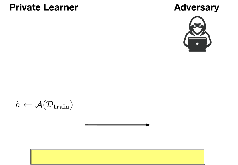
(a) Membership inference attack game

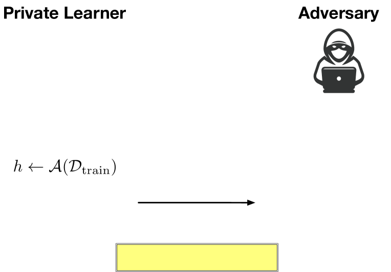
(b) Data reconstruction attack game

Figure 1: Comparison of membership inference attacks (MIAs) and data reconstruction attacks (DRAs). Both attacks are formalized in terms of an attack game between a private learner and an adversary, and the metric of success is given in terms of advantage (Adv; higher is better) for MIA, and mean squared error (MSE; lower is better) for DRA.

Data reconstruction attacks.

Machine learning algorithms often require the model to memorize parts of its training data (Feldman, 2020), enabling adversaries to extract samples from the training dataset when given access to the trained model. Such data reconstruction attacks (DRAs) have been carried out in realistic scenarios against face recognition models (Fredrikson et al., 2015; Zhang et al., 2020) and neural language models (Carlini et al., 2019, 2021), and constitute significant privacy risks for ML models trained on sensitive data.

Differential privacy.

The de facto standard for data privacy in ML is differential privacy (DP), which asserts that for adjacent datasets $\mathcal{D}$ and $\mathcal{D}^{\prime}$ that differ in a single training sample, a model trained on $\mathcal{D}$ is almost statistically indistinguishable from a model trained on $\mathcal{D}^{\prime}$, hence individual samples cannot be reliably inferred. Indistinguishability is measured using a statistical divergence $D$, and a (randomized) learning algorithm $\mathcal{A}$ is differentially private if for any pair of adjacent datasets $\mathcal{D}$ and $\mathcal{D}^{\prime}$, we have $D(\mathcal{A}(\mathcal{D})~{}||~{}\mathcal{A}(\mathcal{D}^{\prime}))\leq\epsilon$ for some fixed privacy parameter $\epsilon>0$. The most common choice for the statistical divergence $D$ is the max divergence:

$$D_{\infty}(P~{}||~{}Q)=\sup_{x\in\mathrm{supp}(Q)}\log\frac{P(x)}{Q(x)},$$

which bounds information leakage in the worst case and is the canonical choice for $\epsilon$-differential privacy (Dwork et al., 2014). The weaker notion of $(\epsilon,\delta)$-DP uses the so-called “hockey-stick” divergence (Polyanskiy et al., 2010), which allows the max divergence bound to fail with probability at most $\delta>0$ (Balle & Wang, 2018). Another generalization uses the Rényi divergence of order $\alpha$ (Rényi, 1961):

$$D_{\alpha}(P~{}||~{}Q)=\frac{1}{\alpha-1}\log\mathbb{E}_{x\sim Q}\left[\left(\frac{P(x)}{Q(x)}\right)^{\alpha}\right]$$

for $\alpha\in(1,\infty)$, and a learning algorithm $\mathcal{A}$ is said to be $(\alpha,\epsilon)$-Rényi differentially private (RDP; Mironov (2017)) if it is DP with respect to the $D_{\alpha}$ divergence. Notably, an $(\alpha,\epsilon)$-RDP mechanism is also $(\epsilon+\log(1/\delta)/(\alpha-1),\delta)$-DP for any $0<\delta<1$ (Mironov, 2017), and RDP is the method of choice for composing multiple mechanisms such as in private SGD (Song et al., 2013; Abadi et al., 2016). More optimal conversions between DP and RDP have been derived by Asoodeh et al. (2021).

Semantic guarantees for differential privacy.

One challenge in applying differential privacy to ML is the selection of the privacy parameter $\epsilon$. For all statistical divergences, the distributions $\mathcal{A}(\mathcal{D})$ and $\mathcal{A}(\mathcal{D}^{\prime})$ are identical when $D(\mathcal{A}(\mathcal{D})~{}||~{}\mathcal{A}(\mathcal{D}^{\prime}))=0$, hence a DP algorithm $\mathcal{A}$ leaks no information about any individual when $\epsilon=0$. However, it is not well-understood at what level of $\epsilon>0$ does the privacy guarantee fail to provide any meaningful protection against attacks (Jayaraman & Evans, 2019).

Several works partially addressed this problem by giving semantic guarantees for DP against membership inference attacks (MIAs; Shokri et al. (2017); Yeom et al. (2018); Salem et al. (2018)). In MIAs, the adversary’s goal is to infer whether a given sample $\mathbf{z}$ participated in the training set $\mathcal{D}$ of a trained model. Formally, the attack can be modeled as a game between a learner and an adversary (see 1(a)), where the membership of a sample is determined by a random bit $b$ and the adversary aims to output a prediction $\hat{b}$ of $b$. The adversary’s metric of success is given by the advantage of the attack, which measures the difference between true and false positive rates of the prediction: $\texttt{Adv}=\mathbb{P}(\hat{b}=0~{}|~{}b=0)-\mathbb{P}(\hat{b}=1~{}|~{}b=0)$. Humphries et al. (2020) showed that if $\mathcal{A}$ is $\epsilon$-DP, then $\texttt{Adv}\leq(e^{\epsilon}-1)/(e^{\epsilon}+1)$. Hence if $\epsilon$ is small, then the adversary cannot perform significantly better than random guessing. For instance, if $\epsilon=0.1$ then the probability of correctly predicting the membership of a sample is at most $(\texttt{Adv}+1)/2\approx 53\%$, which is negligibly better than a random coin flip. Yeom et al. (2018) and Erlingsson et al. (2019) derived similar results.

3 Formalizing Data Reconstruction Attacks

Motivation.

Semantic guarantees for MIA can be useful for interpreting the protection of DP and selecting the privacy parameter $\epsilon$, but several issues remain:

1. Membership status is often not sensitive, but the underlying data value is. For example, a user’s mobile device location can expose the user to unauthorized tracking, but its presence on the network is benign. In these scenarios, it is more meaningful to upper bound how much information can an adversary recover about a training sample.

2. Models trained on complex real-world datasets cannot achieve a low $\epsilon$ while maintaining high utility. Tramèr & Boneh (2020) evaluated different private learning algorithms for training convolutional networks on the MNIST dataset, and showed that practically all current private learning algorithms require $\epsilon\geq 2$ in order to attain a reasonable level of test accuracy. At this $\epsilon$, the attacker’s probability of correcting predicting membership becomes $>88\%$.

3. Data reconstruction is empirically much harder than MIA (Balle et al., 2022), hence it may be possible to derive meaningful guarantees against DRAs even when the membership inference bound becomes vacuous.

Threat model.

Motivated by these shortcomings, we focus on formalizing data reconstruction attacks and deriving semantic guarantees against DRAs for private learning algorithms. 1(b) defines the DRA game, which is a slight modification of the MIA game in 1(a). Let $\mathcal{Z}$ be the data space, and suppose that the learner receives samples $\mathcal{D}\in\mathcal{Z}^{n-1}$ and $\mathbf{z}\in\mathcal{Z}$. Let $\mathcal{D}_{\text{train}}=\mathcal{D}\cup\{\mathbf{z}\}$ be the training dataset, for which the randomized learner outputs a model $h\leftarrow\mathcal{A}(\mathcal{D}_{\text{train}})$ after training on $\mathcal{D}_{\text{train}}$. The adversary receives $h$ and $\mathcal{D}$ and runs the attack algorithm to obtain a reconstruction $\hat{\mathbf{z}}$ of the sample $\mathbf{z}$.

We highlight two major differences between the DRA game and the MIA game: 1. The attack target $\mathbf{z}$ is unknown to the adversary. This change reflects the fact that the adversary’s goal is to reconstruct $\mathbf{z}$ given access to the trained model $h$, rather than infer the membership status of $\mathbf{z}$. 2. The metric of success is $\texttt{MSE}=\mathbb{E}_{h}[\|\hat{\mathbf{z}}-\mathbf{z}\|_{2}^{2}/d]$, where $d$ is the data dimensionality. In other words, the adversary aims to achieve a low reconstruction MSE in expectation over the randomness of the learning algorithm $\mathcal{A}$. Using MSE implicitly assumes that the underlying data is continuous and that the squared difference in $\hat{\mathbf{z}}-\mathbf{z}$ reflects semantic differences. While DRA motivates different metrics of success, we opt to measure MSE in our formulation.

4 Error Bound From RDP

In this section, we show that any RDP learner implies a lower bound on the MSE of a reconstruction attack. Our crucial insight is to view the data reconstruction attack as a parameter estimation problem for the adversary: The sample $\mathbf{z}$ induces a distribution over the space of models through the learning algorithm $\mathcal{A}$. If we treat $\mathbf{z}$ as the parameter of the distribution $\mathcal{A}(\mathcal{D}_{\text{train}})$, we can then utilize statistical estimation theory to lower bound the estimation error of $\mathbf{z}$ when given a single sample from the distribution $\mathcal{A}(\mathcal{D}_{\text{train}})$.

Our main tool for proving this lower bound is the Hammersley-Chapman-Robbins bound (HCRB; Chapman & Robbins (1951)), which we state and prove in Appendix A. Theorem 1 below gives our MSE lower bound for RDP learning algorithms. Proof is given in Appendix B.

Theorem 1.

Let $\mathbf{z}\in\mathcal{Z}\subseteq\mathbb{R}^{d}$ be a sample in the data space $\mathcal{Z}$, and let Att be a reconstruction attack that outputs $\hat{\mathbf{z}}(h)$ upon observing the trained model $h\leftarrow\mathcal{A}(\mathcal{D}_{\text{train}})$, with expectation $\mu(\mathbf{z})=\mathbb{E}_{\mathcal{A}(\mathcal{D}_{\text{train}})}[\hat{\mathbf{z}}(h)]$. If $\mathcal{A}$ is a $(2,\epsilon)$-RDP learning algorithm then:

$$\small\mathbb{E}\left[\|\hat{\mathbf{z}}(h)-\mathbf{z}\|_{2}^{2}/d\right]\geq\underbrace{\frac{\sum_{i=1}^{d}\gamma_{i}^{2}\mathrm{diam}_{i}(\mathcal{Z})^{2}/4d}{e^{\epsilon}-1}}_{\text{variance}}+\underbrace{\frac{\|\mu(\mathbf{z})-\mathbf{z}\|_{2}^{2}}{d}}_{\text{squared bias}},$$

where $\gamma_{i}=\inf_{\mathbf{z}\in\mathcal{Z}}|\partial\mu(\mathbf{z})_{i}/\partial\mathbf{z}_{i}|$ and

$$\mathrm{diam}_{i}(\mathcal{Z})=\sup_{\mathbf{z},\mathbf{z}^{\prime}\in\mathcal{Z}:\mathbf{z}_{j}=\mathbf{z}^{\prime}_{j}\forall j\neq i}|\mathbf{z}_{i}-\mathbf{z}^{\prime}_{i}|$$

is the diameter of $\mathcal{Z}$ in the $i$-th dimension. In particular, if $\hat{\mathbf{z}}(h)$ is unbiased then:

$$\mathbb{E}[\|\hat{\mathbf{z}}(h)-\mathbf{z}\|_{2}^{2}/d]\geq\frac{\sum_{i=1}^{d}\mathrm{diam}_{i}(\mathcal{Z})^{2}/4d}{e^{\epsilon}-1}.$$

Observations.

The semantic guarantee in Theorem 1 has several noteworthy features:

1. There is an explicit bias-variance trade-off for the adversary. The adversary can control its bias-variance trade-off to optimize for MSE, with the trade-off factor determined by $\gamma_{i}$ and $\epsilon$. In essence, $\gamma_{i}$ measures how quickly the adversary’s estimate $\hat{\mathbf{z}}(h)$ changes with respect to $\mathbf{z}$, and the lower bound degrades gracefully with respect to this sensitivity.

2. The variance term is controlled by the privacy parameter $\epsilon$. When $\epsilon=0$, all attacks have infinite variance, which reflects the fact that the adversary can only perform random guessing. As $\epsilon$ increases, the variance term decreases, hence the reconstruction attack can accurately estimate the underlying sample $\mathbf{z}$.

3. The DRA bound can be meaningful even when MIA bounds may not be. Suppose the input space is $\mathcal{Z}=[0,100]$, then $\mathrm{diam}_{1}(\mathcal{Z})=100$. At $\epsilon=2$, the unbiased bound evaluates to $10^{4}/(4(e^{\epsilon}-1))\approx 391$, which means the adversary’s estimate has standard deviation $\approx 19$, i.e., the adversary cannot be certain of their reconstruction up to $\pm 19$. This can be a very meaningful guarantee when the data is only semantically sensitive within a small range, e.g., age.

4. The bound also applies to $\epsilon$-DP. Rényi divergence is non-decreasing in its order $\alpha$ (Sason & Verdú, 2016), i.e., $D_{\alpha}(P~{}||~{}Q)\leq D_{\beta}(P~{}||~{}Q)$ whenever $\alpha\leq\beta$, hence any $\epsilon$-DP mechanism satisfies Theorem 1 as well. Alternative, we can leverage tighter and more general conversions for $(\epsilon,\delta)$-DP (Asoodeh et al., 2021).

Tightness.

The tightness of Theorem 1 has a significant dependence on $\mathrm{diam}_{i}(\mathcal{Z})$. Suppose that $\mathcal{Z}=[0,M]$ for some $M>0$, so $\mathrm{diam}_{1}(\mathcal{Z})=M$. Let $\mathcal{A}(\mathcal{D}_{\text{train}})=z+\mathcal{N}(0,\sigma^{2})$ for any $z\in\mathcal{Z}$, and let $\hat{z}(h)=h$ so that $\hat{z}$ is an unbiased estimator of $z$ with $\mathbb{E}[(\hat{z}(h)-z)^{2}]=\sigma^{2}$. It can be verified that $\mathcal{A}$ satisfies $(2,\epsilon)$-RDP with $\epsilon=M^{2}/\sigma^{2}$, so Theorem 1 gives:

$$\mathbb{E}[(\hat{z}(h)-z)^{2}]\geq\frac{M^{2}}{4(e^{M^{2}/\sigma^{2}}-1)}.$$

As $M\rightarrow 0$, we have that:

$$\lim_{M\rightarrow 0}\frac{M^{2}}{4(e^{M^{2}/\sigma^{2}}-1)}=\lim_{M\rightarrow 0}\frac{2M}{\frac{8M}{\sigma^{2}}e^{M^{2}/\sigma^{2}}}=\sigma^{2}/4,$$

so the bound is tight up to a constant factor. However, it is also clear that this bound converges to $0$ as $M\rightarrow\infty$, hence it can be arbitrarily loose in the worst case. We will show that Fisher information leakage—an alternative measure of privacy loss—can address this worst-case looseness.

5 Error Bound From FIL

Fisher information leakage (FIL; Hannun et al. (2021)) is a recently proposed framework for privacy accounting that is directly inspired by the parameter estimation view of statistical privacy. We show that FIL can be naturally adapted to give a tighter MSE lower bound compared to Theorem 1.

Fisher information leakage.

Fisher information is a statistical measure of information about an underlying parameter from an observable random variable. Suppose that the learning algorithm $\mathcal{A}$ produces a model $h\leftarrow\mathcal{A}(\mathcal{D}_{\text{train}})$ after training on $\mathcal{D}_{\text{train}}=\mathcal{D}\cup\{\mathbf{z}\}$. The Fisher information matrix (FIM) of $h$ about the sample $\mathbf{z}$ is given by:

$$\mathcal{I}_{h}(\mathbf{z})=-\mathbb{E}_{h}\left[\nabla_{\zeta}^{2}\log p_{\mathcal{A}}(h|\zeta)|_{\zeta=\mathbf{z}}\right],$$

where $p_{\mathcal{A}}(h|\zeta)$ denotes the density of $h$ induced by the learning algorithm $\mathcal{A}$ when $\mathbf{z}=\zeta$. For example, if $\mathcal{A}$ trains a linear regressor on $\mathcal{D}_{\text{train}}$ with output perturbation (Chaudhuri et al., 2011), then $p_{\mathcal{A}}(h|\zeta)|_{\zeta=\mathbf{z}}$ is the density function of $\mathcal{N}(\mathbf{w}^{*},\sigma^{2}I_{d})$, with $\mathbf{w}^{*}$ being the unique minimizer of the linear regression objective. Finally, FIL is defined as the spectral norm of the FIM: $\eta^{2}=\|\mathcal{I}_{h}(\mathbf{z})\|_{2}$.

Relationship to differential privacy.

There are close connections between FIL and the statistical divergences used to define DP. Fisher information measures the sensitivity of the density function $p_{\mathcal{A}}(h|\zeta)|_{\zeta=\mathbf{z}}$ with respect to the sample $\mathbf{z}$. If FIL is zero, then the released model $h$ reveals no information about the sample $\mathbf{z}$ since $\mathbf{z}$ does not affect the (log) density of $h$. On the other hand, if FIL is large, then the (log) density of $h$ is very sensitive to change in $\mathbf{z}$, hence revealing a lot of information about $\mathbf{z}$.

It is noteworthy that DP is motivated by a similar reasoning. The divergence bound $D(\mathcal{A}(\mathcal{D}_{\text{train}})~{}||~{}\mathcal{A}(\mathcal{D}_{\text{train}}^{\prime}))$ asserts that the sensitivity of $\mathcal{A}$ to a single sample difference between $\mathcal{D}_{\text{train}}$ and $\mathcal{D}_{\text{train}}^{\prime}$ is small, hence $h$ reveals very little information about any sample in $\mathcal{D}_{\text{train}}$. In fact, it can be shown that Fisher information is the limit of chi-squared divergence (Polyanskiy, 2020): For any $\mathbf{u}\in\mathbb{R}^{d}$,

$$\mathbf{u}^{\top}\mathcal{I}_{h}(\mathbf{z})\mathbf{u}=\lim_{\Delta\rightarrow 0}\chi^{2}(\mathcal{A}(\mathcal{D}\cup\{\mathbf{z}\})~{}||~{}\mathcal{A}(\mathcal{D}\cup\{\mathbf{z}+\Delta\mathbf{u}\})).$$

Since FIL is the spectral norm of $\mathcal{I}_{h}(\mathbf{z})$, it upper bounds the chi-squared divergence between $\mathcal{A}(\mathcal{D}\cup\{\mathbf{z}\})$ and $\mathcal{A}(\mathcal{D}\cup\{\mathbf{z}^{\prime}\})$ as $\mathbf{z}^{\prime}\rightarrow\mathbf{z}$ from any direction. Crucially, this analysis is data-dependent and specific to each $\mathbf{z}\in\mathcal{D}_{\text{train}}$, while preserving the desirable properties of DP such as post-processing inequality (Hannun et al., 2021), composition and subsampling (subsection 6.1).

Cramér-Rao bound.

FIL can be used to lower bound the MSE of DRAs via the Cramér-Rao bound (CRB; Kay (1993))—a well-known result for analyzing the efficiency of estimators (see Appendix A for statement). We adapt the Cramér-Rao bound to prove a similar MSE lower bound as in Theorem 1. Proof is given in Appendix B.

Theorem 2.

Assume the setup of Theorem 1, and additionally that the log density function $\log p_{\mathcal{A}}(h|\zeta)$ satisfies the regularity conditions in Theorem A.2. Then:

$$\mathbb{E}[\|\hat{\mathbf{z}}(h)-\mathbf{z}\|_{2}^{2}/d]\geq$$

$$\quad\quad\underbrace{\frac{\mathrm{Tr}(J_{\mu}(\mathbf{z})\mathcal{I}_{h}(\mathbf{z})^{-1}J_{\mu}(\mathbf{z})^{\top})}{d}}_{\text{variance}}+\underbrace{\frac{\|\mu(\mathbf{z})-\mathbf{z}\|_{2}^{2}}{d}}_{\text{squared bias}}.$$

In particular, if $\hat{\mathbf{z}}(h)$ is unbiased then:

$$\mathbb{E}[\|\hat{\mathbf{z}}(h)-\mathbf{z}\|_{2}^{2}/d]\geq d/\mathrm{Tr}(\mathcal{I}_{h}(\mathbf{z}))\geq 1/\eta^{2}.$$

The bound in Theorem 2 has a similar explicit bias-variance trade-off as that of Theorem 1: The Jacobian $J_{\mu}(\mathbf{z})$ measures how sensitive the estimator $\hat{\mathbf{z}}(h)$ is to $\mathbf{z}$, which interacts with the FIM in the variance term. Notably, the bound for unbiased estimator decays quadratically with respect to the privacy parameter $\eta$ as opposed to exponentially in Theorem 1. We show in section 7 that this scaling also results in tighter MSE lower bounds in practice, yielding a better privacy-utility trade-off for the same private mechanism.

6 Private SGD with FIL Accounting

Private SGD with Gaussian gradient perturbation (Song et al., 2013; Abadi et al., 2016) is a common technique for training DP models, especially neural networks. In this section, we extend FIL accounting to the setting of private SGD by showing analogues of composition and subsampling bounds for FIL. This enables the use of Theorem 2 to derive tighter per-sample estimates of vulnerability to data reconstruction attacks for private SGD learners.

6.1 FIL Accounting for Composition and Subsampling

FIL for a single gradient step.

At time step $t\geq 1$, let $\mathcal{B}_{t}\subseteq\mathcal{D}_{\text{train}}$ be a batch of samples from $\mathcal{D}_{\text{train}}$, and let $\mathbf{w}_{t-1}$ be the model parameters before update. Denote by $\ell(\mathbf{z};\mathbf{w}_{t-1})$ the loss of the model at a sample $\mathbf{z}\in\mathcal{B}_{t}$. Private SGD computes the update (Abadi et al., 2016):

$$\mathbf{g}_{t}(\mathbf{z}) \leftarrow\nabla_{\mathbf{w}}\ell(\mathbf{z};\mathbf{w})|_{\mathbf{w}=\mathbf{w}_{t-1}}\quad\forall\mathbf{z}\in\mathcal{B}_{t}$$

$$\tilde{\mathbf{g}}_{t}(\mathbf{z}) \leftarrow\mathbf{g}_{t}(\mathbf{z})/\max(1,\|\mathbf{g}_{t}(\mathbf{z})\|_{2}/C)$$

$$\bar{\mathbf{g}}_{t} \leftarrow\frac{1}{|\mathcal{B}_{t}|}\left(\sum_{\mathbf{z}\in\mathcal{B}_{t}}\tilde{\mathbf{g}}_{t}(\mathbf{z})+\mathcal{N}(\mathbf{0},\sigma^{2}C^{2}\mathbf{I})\right)$$

$$\mathbf{w}_{t} \leftarrow\mathbf{w}_{t-1}-\rho\bar{\mathbf{g}}_{t}$$

where $\mathbf{I}$ is the identity matrix, $C>0$ is the per-sample clipping norm, $\sigma>0$ is the noise multiplier, and $\rho>0$ is the learning rate. Privacy is preserved using the Gaussian mechanism (Dwork et al., 2014) by adding $\mathcal{N}(\mathbf{0},\sigma^{2}C^{2}\mathbf{I})$ to the aggregate (clipped) gradient $\sum_{\mathbf{z}\in\mathcal{B}_{t}}\tilde{\mathbf{g}}_{t}(\mathbf{z})$. Hannun et al. (2021) showed that the Gaussian mechanism also satisfies FIL privacy, where the FIM is given by:

$$\mathcal{I}_{\bar{\mathbf{g}}_{t}}(\mathbf{z})=\left.\frac{1}{\sigma^{2}}\nabla_{\zeta}\tilde{\mathbf{g}}_{t}(\zeta)^{\top}\nabla_{\zeta}\tilde{\mathbf{g}}_{t}(\zeta)\right|_{\zeta=\mathbf{z}}$$ (1)

for any $\mathbf{z}\in\mathcal{D}_{\text{train}}$. In particular, if $\mathbf{z}\notin\mathcal{B}_{t}$ then $\mathcal{I}_{\bar{\mathbf{g}}_{t}}(\mathbf{z})=0$. The quantity $\nabla_{\zeta}\tilde{\mathbf{g}}_{t}(\zeta)$ is a second-order derivative of the clipped gradient $\tilde{\mathbf{g}}_{t}(\zeta)$, which is computable using popular automatic differentiation packages such as PyTorch (Paszke et al., 2019; Horace He, 2021) and JAX (Bradbury et al., 2018). We will discuss computational aspects of FIL for private SGD in subsection 6.2.

Composition of FIL across multiple gradient steps.

We first consider a simple case for composition where the batches are fixed. Theorem 3 shows that in order to compute the FIM for the final model $h$, it suffices to compute the per-step FIM $\mathcal{I}_{\bar{\mathbf{g}}_{t}}$ and take their sum.

Theorem 3.

Let $\mathbf{w}_{0}$ be the model’s initial parameters, which is drawn independently of $\mathcal{D}_{\text{train}}$. Let $T$ be the total number of iterations of SGD and let $\mathcal{B}_{1},\ldots,\mathcal{B}_{T}$ be a fixed sequence of batches from $\mathcal{D}_{\text{train}}$. Then:

$$\mathcal{I}_{h}(\mathbf{z})\preceq\mathbb{E}_{\mathbf{w}_{0},\bar{\mathbf{g}}_{1},\ldots,\bar{\mathbf{g}}_{T}}\left[\sum_{t=1}^{T}\mathcal{I}_{\bar{\mathbf{g}}_{t}}(\mathbf{z}|\mathbf{w}_{0},\bar{\mathbf{g}}_{1},\ldots,\bar{\mathbf{g}}_{t-1})\right],$$

where $U\preceq V$ means that $V-U$ is positive semi-definite.

Theorem 3 has the following important practical implication: For each realization of $\mathbf{w}_{0},\bar{\mathbf{g}}_{1},\ldots,\bar{\mathbf{g}}_{T}$ (i.e., a single training run), the realized FIM for that run can be computed by summing the per-step FIMs $\mathcal{I}_{\bar{\mathbf{g}}_{t}}$ conditioned on the realized model parameter $\mathbf{w}_{t-1}$ for $t=1,\ldots,T$. This gives an unbiased estimate of an upper bound for $\mathcal{I}_{h}(\mathbf{z})$ via Monte-Carlo, and we can obtain a more accurate upper bound by repeating the training run multiple times and averaging.

Subsampling.

Privacy amplification by subsampling (Kasiviswanathan et al., 2011) is a powerful technique for reducing privacy leakage by randomizing the batches in private SGD: we draw each $\mathcal{B}_{t}$ uniformly from the set of all $B$-subsets of $\mathcal{D}_{\text{train}}$, where $B$ is the batch size. The following theorem shows that private SGD with FIL accounting also enjoys a subsampling amplification bound similar to DP (Abadi et al., 2016) and RDP (Wang et al., 2019; Mironov et al., 2019); the proof is given in Appendix B.

Theorem 4.

Let $\hat{\mathbf{g}}_{t}$ be the perturbed gradient at time step $t$ where the batch $\mathcal{B}_{t}$ is drawn by sampling a subset of size $B$ from $\mathcal{D}_{\text{train}}$ uniformly at random, and let $q=B/|\mathcal{D}_{\text{train}}|$ be the sampling ratio. Then:

$$\mathcal{I}_{\bar{\mathbf{g}}_{t}}(\mathbf{z})\preceq\mathbb{E}_{\mathcal{B}_{t}}[\mathcal{I}_{\bar{\mathbf{g}}_{t}}(\mathbf{z}|\mathcal{B}_{t})].$$ (2)

Furthermore, if the gradient perturbation mechanism is also $\epsilon$-DP, then:

$$\mathcal{I}_{\bar{\mathbf{g}}_{t}}(\mathbf{z})\preceq\frac{q}{q+(1-q)e^{-\epsilon}}\mathbb{E}_{\mathcal{B}_{t}}[\mathcal{I}_{\bar{\mathbf{g}}_{t}}(\mathbf{z}|\mathcal{B}_{t})].$$ (3)

Accounting algorithm.

We can combine Theorem 3 and Theorem 4 to give the full FIL accounting equation for subsampled private SGD:

$$\mathcal{I}_{h}(\mathbf{z})\preceq\mathbb{E}_{\mathbf{w}_{0},\mathcal{B}_{1},\ldots,\mathcal{B}_{T},\bar{\mathbf{g}}_{1},\ldots,\bar{\mathbf{g}}_{T}}\left[\kappa\sum_{t=1}^{T}\mathcal{I}_{\bar{\mathbf{g}}_{t}}(\mathbf{z})\right],$$ (4)

where $\kappa$ is either $1$ or $q/(q+(1-q)e^{-\epsilon})$ depending on which bound in Theorem 4 is used. That is, we perform Monte-Carlo estimation of the FIM by randomizing the initial parameter vector $\mathbf{w}_{0}$ and batches $\mathcal{B}_{1},\ldots,\mathcal{B}_{T}$, and summing up the per-step FIMs. Note that Equation 3 in Theorem 4 depends on the DP privacy parameter $\epsilon$ of the gradient perturbation mechanism. It is well-known that the Gaussian mechanism satisfies $(\epsilon,\delta)$-DP where $\delta>0$ and $\epsilon=2\sqrt{2\log(1.25/\delta)}/\sigma$ (Dwork et al., 2014). Thus, when applying Theorem 4 to private SGD with Gaussian gradient perturbation, there is an arbitrarily small but non-zero probability $\delta$ that the tighter bound in Equation 3 fails, and one must fall back to the simple bound in Equation 2. In practice, we set $\delta$ so that the total failure probability across all iterations $t=1,\ldots,T$ is at most $1/|\mathcal{D}_{\text{train}}|$.

Algorithm 1 FIL computation for private SGD.

1:  Input: Dataset $\mathcal{D}_{\text{train}}$, learning rate $\rho>0$, noise multiplier $\sigma>0$, norm clip threshold $C>0$, failure probability $\delta>0$.

2:  Initialize model parameters $\mathbf{w}_{0}$ independently of $\mathcal{D}_{\text{train}}$.

3:  Initialize FIL accountant $\mathcal{I}(\mathbf{z})=0$ for all $\mathbf{z}\in\mathcal{D}_{\text{train}}$.

4:  $\epsilon\leftarrow 1.115\cdot 2\sqrt{2\log(1.25/\delta)}/\sigma,\;\kappa\leftarrow\frac{q}{q+(1-q)e^{-\epsilon}}$

5:  for $t\leftarrow 1$ to $T$ do

6:     Sample batch $\mathcal{B}_{t}$ uniformly at random from $\mathcal{D}_{\text{train}}$ without replacement.

7:     for $\mathbf{z}\in\mathcal{B}_{t}$ do

8:        $\mathbf{g}_{t}(\mathbf{z})\leftarrow\nabla_{\mathbf{w}}\ell(\mathbf{z};\mathbf{w})|_{\mathbf{w}=\mathbf{w}_{t}}$

9:        $\tilde{\mathbf{g}}_{t}(\mathbf{z})\leftarrow\mathbf{g}_{t}(\mathbf{z})/(\mathrm{GELU}(\|\mathbf{g}_{t}(\mathbf{z})\|_{2}/C-1)+1)$

10:        $\mathcal{I}(\mathbf{z})\leftarrow\mathcal{I}(\mathbf{z})+\left.\frac{\kappa}{\sigma^{2}}\nabla_{\zeta}\tilde{\mathbf{g}}_{t}(\zeta)^{\top}\nabla_{\zeta}\tilde{\mathbf{g}}_{t}(\zeta)\right|_{\zeta=\mathbf{z}}$

11:     end for

12:     $\bar{\mathbf{g}}_{t}\leftarrow\frac{1}{|\mathcal{B}_{t}|}\left(\sum_{\mathbf{z}\in\mathcal{B}_{t}}\tilde{\mathbf{g}}_{t}(\mathbf{z})+\mathcal{N}(\mathbf{0},\sigma^{2}C^{2}\mathbf{I})\right)$

13:     $\mathbf{w}_{t}\leftarrow\mathbf{w}_{t-1}-\rho\bar{\mathbf{g}}_{t}$

14:  end for

15:  Return: Fisher information upper bound $\{\mathcal{I}(\mathbf{z})\}_{\mathbf{z}\in\mathcal{D}_{\text{train}}}$.

6.2 Computing FIL

Handling non-differentiability.

The core quantity in FIL accounting is the per-step FIM of the gradient in Equation 1, which involves computing a second-order derivative $\nabla_{\zeta}\tilde{\mathbf{g}}_{t}(\zeta)$ whose existence depends on the loss $\ell(\mathbf{z};\mathbf{w})$ being differentiable everywhere in both $\mathbf{z}$ and $\mathbf{w}$. This is not always the case since: 1. The network may have non-differentiable activation functions such as ReLU; and 2. The gradient norm clip operator requires computing $\max(1,\|\mathbf{g}_{t}(\mathbf{z})\|_{2}/C)$, which is also non-differentiable.

We address the first problem by replacing ReLU with the $\tanh$ activation function, which is smooth and has been recently found to be more suitable for private SGD training (Papernot et al., 2020). The second problem can be addressed using the GELU function (Hendrycks & Gimpel, 2016), which is a smooth approximation to $\max(0,z)$. In particular, we replace the $\max(1,z)$ function with $\mathrm{GELU}(z-1)+1$.

Algorithm 1 summarizes the FIL computation with this modified norm clip operator in pseudo-code. We substitute hard gradient norm clipping using GELU in line 9. It can be verified that gradient norm clipping using GELU introduces a small multiplicative overhead in the clipping threshold: $\|\tilde{\mathbf{g}}_{t}(\mathbf{z})\|_{2}\leq 1.115C$ if $\tilde{\mathbf{g}}_{t}(\mathbf{z})=\mathbf{g}_{t}(\mathbf{z})/(\mathrm{GELU}(\|\mathbf{g}_{t}(\mathbf{z})\|_{2}/C-1)+1)$.

Improving computational efficiency.

Computation of the second-order derivative $\nabla_{\zeta}\tilde{\mathbf{g}}_{t}(\zeta)$ can be done in JAX (Bradbury et al., 2018) using the jacrev operator. However, the dimensionality of the derivative $\nabla_{\zeta}\tilde{\mathbf{g}}_{t}(\zeta)$ is $p\times d$, where $p$ is the number of model parameters and $d$ is the data dimensionality, which can be too costly to store in memory. Fortunately, the bound for unbiased estimator in Theorem 2 only requires computing either the trace or the spectral norm of $\mathcal{I}_{\bar{\mathbf{g}}_{t}}(\mathbf{z})$, which does not require instantiating the full second-order derivative $\nabla_{\zeta}\tilde{\mathbf{g}}_{t}(\zeta)$. For instance,

$$\mathrm{Tr}(\mathcal{I}_{\bar{\mathbf{g}}_{t}}(\mathbf{z}))=\sum_{i=1}^{d}\mathbf{e}_{i}^{\top}\mathcal{I}_{\bar{\mathbf{g}}_{t}}(\mathbf{z})\mathbf{e}_{i}=\sum_{i=1}^{d}\frac{\|\nabla_{\zeta}\tilde{\mathbf{g}}_{t}(\zeta)\mathbf{e}_{i}|_{\zeta=\mathbf{z}}\|_{2}^{2}}{\sigma^{2}},$$ (5)

which can be computed using only Jacobian-vector products (jvp in JAX) without constructing the full Jacobian matrix. This can be done in Algorithm 1 by modifying Line 10 accordingly. Furthermore, we can obtain an unbiased estimate of $\mathrm{Tr}(\mathcal{I}_{\bar{\mathbf{g}}_{t}}(\mathbf{z}))$ by sampling the coordinates $i=1,\ldots,d$ in Equation 5 stochastically. Doing so gives a Monte-Carlo estimate of $\mathrm{Tr}(\mathcal{I}_{h}(\mathbf{z}))$ using Equation 4 since trace is a linear operator. Similarly, we can compute the spectral norm using JVP via power iteration.

7 Experiments

We evaluate our MSE lower bounds in Theorem 1 and Theorem 2 for unbiased estimators and show that RDP and FIL both provide meaningful semantic guarantees against DRAs. In addition, we evaluate the informed adversary attack (Balle et al., 2022) against privately trained models and show that a sample’s vulnerability to this reconstruction attack is closely captured by the FIL lower bound. Code to reproduce our results is available at https://github.com/facebookresearch/bounding_data_reconstruction.

7.1 Linear Logistic Regression

We first consider linear logistic regression for binary MNIST (LeCun et al., 1998) classification of digits $0$ vs. $1$. The training set contains $n=12,665$ samples. Each sample $\mathbf{z}=(\mathbf{x},y)$ consists of an input image $\mathbf{x}\in[0,1]^{784}$ and a label $y\in\{0,1\}$. Since the value of $y$ is discrete, we treat the label as public and only seek to prevent reconstruction of the image $\mathbf{x}$.

Privacy accounting.

The linear logistic regressor is trained privately using output perturbation (Chaudhuri et al., 2011) by adding Gaussian noise $\mathcal{N}(0,\sigma^{2}\mathbf{I})$ to the non-private model. For a given L2 regularization parameter $\lambda>0$ and noise parameter $\sigma>0$, it can be shown that output perturbation satisfies $(2,\epsilon)$-RDP with $\epsilon=4/(n\lambda\sigma)^{2}$. For FIL accounting, we follow Hannun et al. (2021) and compute the full Fisher information matrix $\mathcal{I}_{h}(\mathbf{z})$, then take the average diagonal value $\bar{\eta}^{2}:=\mathrm{Tr}(\mathcal{I}_{h}(\mathbf{z}))/d$ in order to apply Theorem 2. The final estimate is computed as an average across 10 runs. We refer to this quantity as the diagonal Fisher information loss (dFIL).

Result.

We train the model with $\lambda=10^{-2}$ and $\sigma=10^{-2}$, achieving a near-perfect test accuracy of $99.95\%$ and $(2,\epsilon)$-RDP with $\epsilon=2.49$. Figure 2 shows the RDP lower bound in Theorem 1 and the histogram of per-sample dFIL lower bounds in Theorem 2. Since the data space is $[0,1]^{784}$, we have that $\mathrm{diam}_{i}(\mathcal{Z})=1$ for all $i$, so the RDP bound reduces to $\texttt{MSE}\geq 1/(4(e^{\epsilon}-1))$, while the dFIL bound is $\texttt{MSE}\geq 1/\bar{\eta}^{2}$. The plot shows that the RDP bound is $\approx 0.02$, while all the per-sample dFIL bounds are $>1$. Since $\texttt{MSE}\leq 1$ can be achieved by simply guessing any value within $[0,1]^{784}$, we regard the vertical line of $\texttt{MSE}=1$ as perfect privacy. Hence the dFIL predicts that all training samples are safe from reconstruction attacks. Moreover, there is an extremely wide range of values for the per-sample dFIL bounds. We show in the following experiment that these values are highly indicative of how susceptible the sample is to an actual data reconstruction attack.

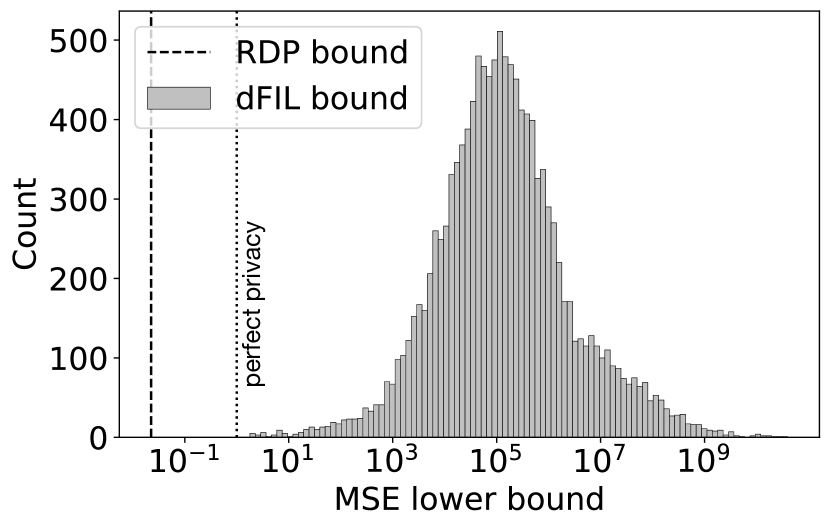
Figure 2: Plot showing the RDP lower bound and histogram of the per-sample FIL lower bound for the MNIST 0 vs. 1 classifier. The vertical line at $\texttt{MSE}=1$ represents the perfect privacy threshold, which is the MSE attainable by a random guessing adversary.

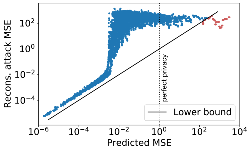
Figure 3: Scatter plot of the MSE lower bound from FIL (x-axis) and the MSE realized by the GLM attack (y-axis; Balle et al. (2022)). The MSE lower bound predicted by Theorem 2 is highly indicative of the sample’s vulnerability to the GLM attack.

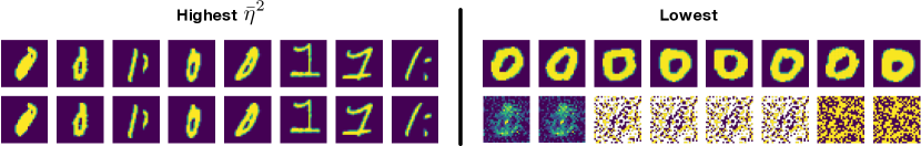
Figure 4: Training samples (top row) and their reconstructions (bottom row) by the GLM attack. Samples are sorted in decreasing order of the dFIL $\bar{\eta}^{2}$. Samples with high dFIL can be reconstructed perfectly, while ones with low dFIL are protected against the GLM attack.

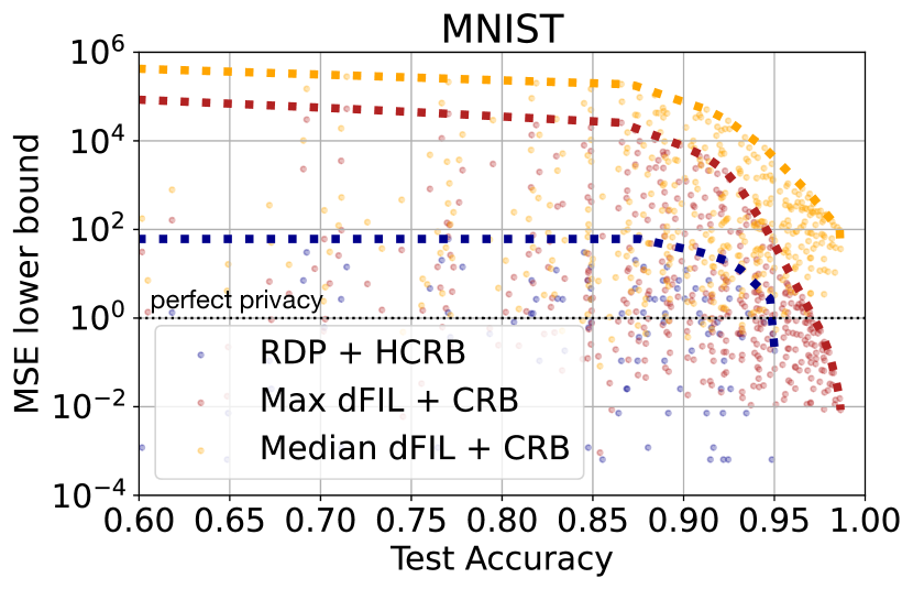
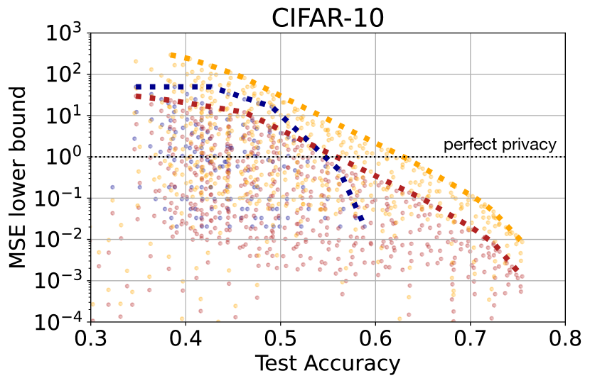
Figure 5: Comparison of MSE lower bounds from RDP and FIL. Dashed line shows the optimal privacy-utility trade-off across all searched hyperparameters. The maximum dFIL across the dataset gives a better MSE lower bound compared to the RDP bound in most settings.

7.2 Lower Bounding Reconstruction Attack

Balle et al. (2022) proposed a strong data reconstruction attack against generalized linear models (GLMs). We strengthen the attack by providing the label $y$ of the target sample $\mathbf{z}=(\mathbf{x},y)$ to the adversary in addition to all other samples in $\mathcal{D}_{\text{train}}$. To evaluate the GLM attack, we train a private model using output perturbation with $\lambda=10^{-2}$ and $\sigma=10^{-5}$, and apply the GLM attack to reconstruct each sample in the training set. We repeat this process $10,000$ times and compute the expected MSE across the trials. The noise parameter $\sigma$ is intentionally set to be very small to enable data reconstruction on some vulnerable samples. Under this setting, the model is $(2,\epsilon)$-RDP with $\epsilon=2.5\times 10^{6}$, which is too large to provide any meaningful privacy guarantee.

Result.

Figure 3 shows the scatter plot of MSE lower bounds predicted by the dFIL bound (x-axis) vs. the realized expected MSE of the GLM attack (y-axis). The solid line shows the cut-off for the dFIL lower bound, hence all points should be above the solid line if the dFIL bound holds. We see that this is indeed the case for the majority of samples: lower predicted MSE corresponds to lower realized MSE, and there is a close correlation between the two values especially at the lower end. We observe that some samples (highlighted in red) violate the dFIL lower bound. One explanation is that the GLM attack incurs a high bias when the sample is hard to reconstruct, hence the unbiased bound in Theorem 2 fails to hold for those samples. Nevertheless, we see that for all samples with $\texttt{MSE}\leq 1$ (to the left of the perfect privacy line), the dFIL bound does provide a meaningful semantic guarantee against the GLM attack.

Reconstructed samples.

Figure 4 shows selected training samples (top row) and their reconstructions (bottom row). Samples are sorted in decreasing order of dFIL $\bar{\eta}^{2}$ and only the top- and bottom-8 are shown. For samples with the highest dFIL (i.e., lowest MSE bounds), the GLM attack successfully reconstructs the sample, while the attack fails for samples with the lowest dFIL.

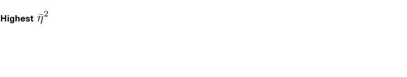
Figure 6: CIFAR-10 training samples with the highest and lowest dFIL values $\bar{\eta}$.

7.3 Neural Networks

Finally, we compare MSE lower bounds for RDP and FIL accounting for the private SGD learner. We train two distinct convolutional networks on the full 10-digit MNIST (LeCun et al., 1998) dataset and the CIFAR-10 (Krizhevsky et al., 2009) dataset. The learner has several hyperparameters, and we exhaustively evaluate on all hyperparameter settings via grid search; see Appendix C for details. Similar to the experiment in subsection 7.1, we treat the label as public and compute MSE bounds for reconstructing the input $\mathbf{x}$.

Privacy accounting.

For RDP accounting, we apply the subsampling bound in Mironov et al. (2019). For FIL accounting we use Algorithm 1, and estimate $\mathrm{Tr}(\mathcal{I}_{\tilde{\mathbf{g}}_{t}}(\mathbf{z}))$ by sampling $50$ coordinates randomly every iteration (see Equation 5). Failure probability for the subsampling bound in Equation 3 is set to $\delta<10^{-5}$. Each training run is repeated $10$ times to give a Monte-Carlo estimate for dFIL.

Result.

Figure 5 shows the MSE lower bounds from RDP and dFIL on MNIST (left) and CIFAR-10 (right). Each point in the scatter plot corresponds to a single hyperparameter configuration, where we show the test accuracy on the x-axis and the MSE lower bound on the y-axis. In addition, we show the Pareto frontier using the dashed line, which indicates the optimal privacy-utility trade-off found by the grid search. In both plots, the RDP bound (shown in blue) gives a meaningful MSE lower bound, where the model can attain a reasonable accuracy ($95\%$ for MNIST and $55\%$ for CIFAR-10) before crossing the perfect privacy threshold.

The dFIL bound paints a more optimistic picture: For the same private mechanism, the maximum dFIL across the training set (shown in red) combined with Theorem 2 gives an MSE lower bound that is orders of magnitude higher than the RDP bound at higher accuracies. On MNIST, the model can attain $97\%$ test accuracy before crossing the perfect privacy threshold. On CIFAR-10, although the dFIL bound crosses the perfect privacy threshold at approximately the same accuracy as the RDP bound, the bound deteriorates much more gradually, giving a non-negligible privacy guarantee of $\texttt{MSE}\geq 0.1$ at test accuracy $64\%$. Moreover, the median dFIL (shown in orange) indicates that even at high levels of accuracy, the median MSE lower bound across the dataset remains relatively high, hence most training samples are still safe from reconstruction attacks.

CIFAR-10 samples.

Figure 6 shows CIFAR-10 training samples with the highest and lowest privacy leakage according to dFIL ($\bar{\eta}$; shown above each image) for a ConvNet model trained privately with $T=5000,\sigma=0.5,\rho=0.1$ and $C=1$. Qualitatively, samples with low privacy leakage (bottom row) are typical images for their class and are easy to recognize, while samples with high privacy leakage (top row) are difficult to classify correctly even for humans.

8 Discussion

We presented a formal framework for analyzing data reconstruction attacks, and proved two novel lower bounds on the MSE of reconstructions for private learners using RDP and FIL accounting. Our work also extended FIL accounting to private SGD, and we showed that the resulting MSE lower bounds drastically improve upon those derived from RDP. We hope that future research can build upon our work to develop more comprehensive analytical tools for evaluating the privacy risks of learning algorithms.

Concurrent work by Balle et al. (2022) offered a Bayesian approach to bounding reconstruction attacks. Their formulation lower bounds the reconstruction error of an adversary in terms of the error of an adversary with only access to the data distribution prior and the DP parameter $\epsilon$. In contrast, our bounds characterize the prior of an adversary in terms of sensitivity of their estimate to the training data, with a priorless adversary being unbiased and hence the most sensitive. Interestingly, the Bayesian extension (Van Trees, 2004) of the Cramér-Rao bound used in our result offers a similar interpretation as Balle et al. (2022), and we hope to unite these two interpretations in future work.

Limitations.

Our work presents several opportunities for further improvement.

1. The RDP bound only applies natively for order $\alpha=2$. To extend it to general order $\alpha$, one promising direction is to use minimax bounds (Rigollet & Hütter, 2015) to establish a relationship between parameter estimation and hypothesis testing, which enables the use of general DP accountants to derive MSE lower bounds for DRAs.

2. Computing the FIM requires evaluating a second-order derivative, which is much more expensive (in terms of both compute and memory) to derive than simpler quantities such as Rényi divergence. Improvements in this aspect can enable the use of the FIL accountant in larger models.

3. We empirically evaluated both the RDP and FIL lower bounds only for unbiased adversaries. In practice, data reconstruction attacks can leverage informative priors such as the smoothness prior for images, and hence are unlikely to be truly unbiased. Further investigation into MSE lower bounds for biased estimators can enable more robust semantic guarantees against data reconstruction attacks.

Appendix A Cramér-Rao and Hammersley-Chapman-Robbins Bounds

Below, we state the Cramér-Rao Bound (CRB) and the Hammersley-Chapman-Robbins Bound (HCRB)—two cornerstone results in statistics that we leverage for proving our main results.

Theorem A.1 (Hammersley-Chapman-Robbins Bound).

Let $\theta\in\Theta\subseteq\mathbb{R}^{d}$ be a parameter vector and let $U$ be a random variable whose density function $p(\mathbf{u};\theta)$ is parameterized by $\theta$ and is positive for all $\mathbf{u}\in\mathbb{R}^{p}$ and $\theta\in\Theta$. Let $\hat{\theta}(U)$ be an estimator of $\theta$ whose expectation is $\mu(\theta):=\mathbb{E}_{U\sim p(\mathbf{u};\theta)}[\hat{\theta}(U)]$. Then for any $i\in\{1,\ldots,d\}$ and $\Delta\in\mathbb{R}$, we have that:

$$\operatorname{Var}\left(\hat{\theta}(U)_{i}\right)\geq\frac{\quad(\mu(\theta+\Delta\mathbf{e}_{i})_{i}-\mu(\theta)_{i})^{2}}{\chi^{2}(p(\mathbf{u};\theta+\Delta\mathbf{e}_{i})~{}||~{}p(\mathbf{u};\theta))},$$

where $\mathbf{e}_{i}$ is the standard basis vector with $i$th coordinate equal to 1, and $\chi^{2}(P~{}||~{}Q)=\mathbb{E}_{Q}[(P/Q-1)^{2}]$ is the chi-squared divergence between $P$ and $Q$.

Proof.

First note that

$$\mu(\theta+\Delta\mathbf{e}_{i})-\mu(\theta) =\mathbb{E}_{U\sim p(\mathbf{u};\theta+\Delta\mathbf{e}_{i})}[\hat{\theta}(U)-\mu(\theta)]-\mathbb{E}_{U\sim p(\mathbf{u};\theta)}[\hat{\theta}(U)-\mu(\theta)]$$

$$=\mathbb{E}_{U\sim p(\mathbf{u};\theta)}\left[(\hat{\theta}(U)-\mu(\theta))\frac{p(\mathbf{u};\theta+\Delta\mathbf{e}_{i})-p(\mathbf{u};\theta)}{p(\mathbf{u};\theta)}\right].$$

Squaring and applying Cauchy-Schwarz gives

$$(\mu(\theta+\Delta\mathbf{e}_{i})_{i}-\mu(\theta)_{i})^{2} \leq\mathbb{E}_{U\sim p(\mathbf{u};\theta)}\left[(\hat{\theta}(U)_{i}-\mu(\theta)_{i})^{2}\right]\mathbb{E}_{U\sim p(\mathbf{u};\theta)}\left[\left(\frac{p(\mathbf{u};\theta+\Delta\mathbf{e}_{i})-p(\mathbf{u};\theta)}{p(\mathbf{u};\theta)}\right)^{2}\right]$$

$$=\operatorname{Var}(\hat{\theta}(U)_{i})\chi^{2}(p(\mathbf{u};\theta+\Delta\mathbf{e}_{i})~{}||~{}p(\mathbf{u};\theta)),$$

as desired. ∎

Theorem A.2 (Cramér-Rao Bound).

Assume the setup of Theorem A.1, and additionally that the log density function $\log p(\mathbf{u};\theta)$ is twice differentiable and satisfies the following regularity condition: $\mathbb{E}[\partial\log p(\mathbf{u};\theta)/\partial\theta]=0$ for all $\theta$. Let $\mathcal{I}_{U}(\theta)$ be the Fisher information matrix of $U$ for the parameter vector $\theta$. Then the estimator $\hat{\theta}(U)$ satisfies:

$$\operatorname{Var}\left(\hat{\theta}(U)\right)\succeq J_{\mu}(\theta)\mathcal{I}_{U}(\theta)^{-1}J_{\mu}(\theta)^{\top},$$

where $J_{\mu}(\theta)$ is the Jacobian of $\mu$ with respect to $\theta$.

Appendix B Proofs

We present proofs of theoretical results from the main text.

Theorem 1.

Let $\mathbf{z}\in\mathcal{Z}\subseteq\mathbb{R}^{d}$ be a sample in the data space $\mathcal{Z}$, and let Att be a reconstruction attack that outputs $\hat{\mathbf{z}}(h)$ upon observing the trained model $h\leftarrow\mathcal{A}(\mathcal{D}_{\text{train}})$, with expectation $\mu(\mathbf{z})=\mathbb{E}_{\mathcal{A}(\mathcal{D}_{\text{train}})}[\hat{\mathbf{z}}(h)]$. If $\mathcal{A}$ is a $(2,\epsilon)$-RDP learning algorithm then:

$$\mathbb{E}\left[\|\hat{\mathbf{z}}(h)-\mathbf{z}\|_{2}^{2}/d\right]\geq\underbrace{\frac{\sum_{i=1}^{d}\gamma_{i}^{2}\mathrm{diam}_{i}(\mathcal{Z})^{2}/4d}{e^{\epsilon}-1}}_{\text{variance}}+\underbrace{\frac{\|\mu(\mathbf{z})-\mathbf{z}\|_{2}^{2}}{d}}_{\text{squared bias}},$$

where $\gamma_{i}=\inf_{\mathbf{z}\in\mathcal{Z}}|\partial\mu(\mathbf{z})_{i}/\partial\mathbf{z}_{i}|$ and

$$\mathrm{diam}_{i}(\mathcal{Z})=\sup_{\mathbf{z},\mathbf{z}^{\prime}\in\mathcal{Z}:\mathbf{z}_{j}=\mathbf{z}^{\prime}_{j}\forall j\neq i}|\mathbf{z}_{i}-\mathbf{z}^{\prime}_{i}|$$

is the diameter of $\mathcal{Z}$ in the $i$-th dimension. In particular, if $\hat{\mathbf{z}}(h)$ is unbiased then:

$$\mathbb{E}[\|\hat{\mathbf{z}}(h)-\mathbf{z}\|_{2}^{2}/d]\geq\frac{\sum_{i=1}^{d}\mathrm{diam}_{i}(\mathcal{Z})^{2}/4d}{e^{\epsilon}-1}.$$

Proof.

Let $p(h;\mathbf{z}^{\prime})$ be the density of $h\leftarrow\mathcal{A}(\mathcal{D}_{\text{train}})$ when $\mathcal{D}_{\text{train}}=\mathcal{D}\cup\{\mathbf{z}^{\prime}\}$. We first invoke the well-known identity $D_{2}(P~{}||~{}Q)=\log(1+\chi^{2}(P~{}||~{}Q))$, hence if $\mathcal{A}$ is $(2,\epsilon)$-RDP then $\chi^{2}(p(h;\mathbf{z}+\Delta\mathbf{e}_{i})~{}||~{}p(h;\mathbf{z}))\leq e^{\epsilon}-1$. For each $i=1,\ldots,d$, we can apply bias-variance decomposition to get $(\hat{\mathbf{z}}(h)_{i}-\mathbf{z}_{i})^{2}=\operatorname{Var}(\hat{\mathbf{z}}(h)_{i})+(\mu(\mathbf{z})_{i}-\mathbf{z}_{i})^{2}$. Applying Theorem A.1 to the variance term gives:

$$\operatorname{Var}(\hat{\mathbf{z}}(h)_{i}) \geq(\mu(\mathbf{z}+\Delta\mathbf{e}_{i})_{i}-\mu(\mathbf{z})_{i})^{2}/\chi^{2}(p(h;\mathbf{z}+\Delta\mathbf{e}_{i})~{}||~{}p(h;\mathbf{z}))$$

$$\geq(\mu(\mathbf{z}+\Delta\mathbf{e}_{i})_{i}-\mu(\mathbf{z})_{i})^{2}/(e^{\epsilon}-1)$$

$$\geq\gamma_{i}^{2}\Delta^{2}/(e^{\epsilon}-1),$$

where the last inequality follows from the mean value theorem. Since this holds for any $\Delta$, we can maximize over $\{\Delta\in\mathbb{R}:\mathbf{z}+\Delta\mathbf{e}_{i}\in\mathcal{Z}\}$, which gives $\operatorname{Var}(\hat{\mathbf{z}}(h)_{i})\geq\gamma_{i}^{2}\mathrm{diam}_{i}(\mathcal{Z})^{2}/4(e^{\epsilon}-1)$. Summing over $i=1,\ldots,d$ gives the desired bound. If $\hat{\mathbf{z}}(h)$ is unbiased then $\mu(\mathbf{z})=\mathbf{z}$ and $\gamma_{i}=1$ for all $i$, thus $\mathbb{E}[\|\hat{\mathbf{z}}(h)-\mathbf{z}\|_{2}^{2}/d]\geq\frac{\sum_{i=1}^{d}\mathrm{diam}_{i}(\mathcal{Z})^{2}/4d}{e^{\epsilon}-1}$. ∎

Theorem 2.

Assume the setup of Theorem 1, and additionally that the log density function $\log p_{\mathcal{A}}(h|\zeta)$ satisfies the conditions in Theorem A.2. Then:

$$\mathbb{E}[\|\hat{\mathbf{z}}(h)-\mathbf{z}\|_{2}^{2}/d]\geq\underbrace{\frac{\mathrm{Tr}(J_{\mu}(\mathbf{z})\mathcal{I}_{h}(\mathbf{z})^{-1}J_{\mu}(\mathbf{z})^{\top})}{d}}_{\text{variance}}+\underbrace{\frac{\|\mu(\mathbf{z})-\mathbf{z}\|_{2}^{2}}{d}}_{\text{squared bias}}.$$

In particular, if $\hat{\mathbf{z}}(h)$ is unbiased then:

$$\mathbb{E}[\|\hat{\mathbf{z}}(h)-\mathbf{z}\|_{2}^{2}/d]\geq d/\mathrm{Tr}(\mathcal{I}_{h}(\mathbf{z}))\geq 1/\eta^{2}.$$

Proof.

The general bound for biased estimators follows directly from Theorem A.2 and bias-variance decomposition of MSE. For the unbiased estimator bound, note that the Jacobian $J_{\mu}(\mathbf{z})=I_{d}$, so

$$\mathbb{E}[\|\hat{\mathbf{z}}(h)-\mathbf{z}\|_{2}^{2}/d]\geq\mathrm{Tr}(\mathcal{I}_{h}(\mathbf{z})^{-1})/d\geq d^{2}\mathrm{Tr}(\mathcal{I}_{h}(\mathbf{z}))^{-1}/d=d/\mathrm{Tr}(\mathcal{I}_{h}(\mathbf{z})),$$

where the second inequality follows from Cauchy-Schwarz. Finally, $\mathrm{Tr}(\mathcal{I}_{h}(\mathbf{z}))=\sum_{i=1}^{d}\mathbf{e}_{i}^{\top}\mathcal{I}_{h}(\mathbf{z})\mathbf{e}_{i}\leq\sum_{i=1}^{d}\eta^{2}\|\mathbf{e}_{i}\|_{2}^{2}=d\eta^{2}$, and the result follows. ∎

Theorem 3.

Let $\mathbf{w}_{0}$ be the model’s initial parameters, which is drawn independently of $\mathcal{D}_{\text{train}}$. Let $T$ be the total number of iterations of SGD and let $\mathcal{B}_{1},\ldots,\mathcal{B}_{T}$ be a fixed sequence of batches from $\mathcal{D}_{\text{train}}$. Then:

$$\mathcal{I}_{\mathbf{w}_{0},\bar{\mathbf{g}}_{1},\ldots,\bar{\mathbf{g}}_{T}}(\mathbf{z})\preceq\mathbb{E}_{\mathbf{w}_{0},\bar{\mathbf{g}}_{1},\ldots,\bar{\mathbf{g}}_{T}}\left[\sum_{t=1}^{T}\mathcal{I}_{\bar{\mathbf{g}}_{t}}(\mathbf{z}|\mathbf{w}_{0},\bar{\mathbf{g}}_{1},\ldots,\bar{\mathbf{g}}_{t-1})\right],$$

where $U\preceq V$ means that $V-U$ is positive semi-definite.

Proof.

First note that the final model $h\leftarrow\mathcal{A}(\mathcal{D}_{\text{train}})$ is a deterministic function of only the initial parameters $\mathbf{w}_{0}$ and the observed gradients $\bar{\mathbf{g}}_{1},\ldots,\bar{\mathbf{g}}_{T}$ without any other access to $\mathbf{z}$, hence by the post-processing inequality for Fisher information (Zamir, 1998), we get $\mathcal{I}_{h}(\mathbf{z})\preceq\mathcal{I}_{\mathbf{w}_{0},\bar{\mathbf{g}}_{1},\ldots,\bar{\mathbf{g}}_{T}}(\mathbf{z})$. To bound $\mathcal{I}_{\mathbf{w}_{0},\bar{\mathbf{g}}_{1},\ldots,\bar{\mathbf{g}}_{T}}(\mathbf{z})$ for any $\mathbf{z}\in\mathcal{D}_{\text{train}}$, we apply the chain rule for Fisher information (Zamir, 1998):

$$\mathcal{I}_{\mathbf{w}_{0},\bar{\mathbf{g}}_{1},\ldots,\bar{\mathbf{g}}_{T}}(\mathbf{z}) =\mathcal{I}_{\mathbf{w}_{0}}(\mathbf{z})+\mathbb{E}_{\mathbf{w}_{0},\bar{\mathbf{g}}_{1},\ldots,\bar{\mathbf{g}}_{T}}\left[\sum_{t=1}^{T}\mathcal{I}_{\bar{\mathbf{g}}_{t}}(\mathbf{z}|\mathbf{w}_{0},\bar{\mathbf{g}}_{1},\ldots,\bar{\mathbf{g}}_{t-1})\right]$$

$$=\mathbb{E}_{\mathbf{w}_{0},\bar{\mathbf{g}}_{1},\ldots,\bar{\mathbf{g}}_{T}}\left[\sum_{t=1}^{T}\mathcal{I}_{\bar{\mathbf{g}}_{t}}(\mathbf{z}|\mathbf{w}_{0},\bar{\mathbf{g}}_{1},\ldots,\bar{\mathbf{g}}_{t-1})\right],$$

where $\mathcal{I}_{\mathbf{w}_{0}}(\mathbf{z})=0$ since $\mathbf{w}_{0}$ is independent of the training data. The quantity $\mathcal{I}_{\bar{\mathbf{g}}_{t}}(\mathbf{z}|\mathbf{w}_{0},\bar{\mathbf{g}}_{1},\ldots,\bar{\mathbf{g}}_{t-1})$ represents the conditional Fisher information, which depends on the current model parameter $\mathbf{w}_{t-1}$ through $\mathbf{w}_{0},\bar{\mathbf{g}}_{1},\ldots,\bar{\mathbf{g}}_{t-1}$. ∎

Theorem 4.

Let $\hat{\mathbf{g}}_{t}$ be the perturbed gradient at time step $t$ where the batch $\mathcal{B}_{t}$ is drawn by sampling a subset of size $B$ from $\mathcal{D}_{\text{train}}$ uniformly randomly, and let $q=B/|\mathcal{D}_{\text{train}}|$ be the sampling ratio. Then:

$$\mathcal{I}_{\bar{\mathbf{g}}_{t}}(\mathbf{z})\preceq\mathbb{E}_{\mathcal{B}_{t}}[\mathcal{I}_{\bar{\mathbf{g}}_{t}}(\mathbf{z}|\mathcal{B}_{t})].$$

Furthermore, if the gradient perturbation mechanism is also $\epsilon$-DP, then:

$$\mathcal{I}_{\bar{\mathbf{g}}_{t}}(\mathbf{z})\preceq\frac{q}{q+(1-q)e^{-\epsilon}}\mathbb{E}_{\mathcal{B}_{t}}[\mathcal{I}_{\bar{\mathbf{g}}_{t}}(\mathbf{z}|\mathcal{B}_{t})].$$

Proof.

The first bound follows from convexity of Fisher information. Let $\mathcal{B}_{t}^{1}$ and $\mathcal{B}_{t}^{2}$ be two batches and let $p_{1},p_{2}$ be the density functions of the perturbed batch gradient $\bar{\mathbf{g}}_{t}$ corresponding to the two batches. For any $\lambda\in(0,1)$, let $\mathcal{I}_{\bar{\mathbf{g}}_{t}}(\mathbf{z})$ be the FIM for the mixture distribution with $\mathbb{P}(\mathcal{B}_{t}^{1})=\lambda$ and $\mathbb{P}(\mathcal{B}_{t}^{2})=1-\lambda$. We will show that:

$$\mathcal{I}_{\bar{\mathbf{g}}_{t}}(\mathbf{z})\preceq\lambda\mathcal{I}_{\bar{\mathbf{g}}_{t}}(\mathbf{z}|\mathcal{B}_{t}^{1})+(1-\lambda)\mathcal{I}_{\bar{\mathbf{g}}_{t}}(\mathbf{z}|\mathcal{B}_{t}^{2}).$$ (6)

For any $\mathbf{u}\in\mathbb{R}^{p}$, observe that:

$$\mathbf{u}^{\top}\mathcal{I}_{\bar{\mathbf{g}}_{t}}(\mathbf{z}|\mathcal{B}_{t}^{1})\mathbf{u} =\int_{\bar{\mathbf{g}}_{t}}\mathbf{u}^{\top}\left[\left.\nabla_{\zeta}\log p_{1}(\bar{\mathbf{g}}_{t}|\zeta)\nabla_{\zeta}\log p_{1}(\bar{\mathbf{g}}_{t}|\zeta)^{\top}\right|_{\zeta=\mathbf{z}}\right]\mathbf{u}\>p_{1}(\bar{\mathbf{g}}_{t}|\zeta)\;d\bar{\mathbf{g}}_{t}$$

$$=\int_{\bar{\mathbf{g}}_{t}}\mathbf{u}^{\top}\left[\left.\nabla_{\zeta}p_{1}(\bar{\mathbf{g}}_{t}|\zeta)\nabla_{\zeta}p_{1}(\bar{\mathbf{g}}_{t}|\zeta)^{\top}\right|_{\zeta=\mathbf{z}}\right]\mathbf{u}/p_{1}(\bar{\mathbf{g}}_{t}|\zeta)\;d\bar{\mathbf{g}}_{t}$$

$$=\int_{\bar{\mathbf{g}}_{t}}[p_{1,\mathbf{u}}^{\prime}(\bar{\mathbf{g}}_{t}|\zeta)|_{\zeta=\mathbf{z}}]^{2}/p_{1}(\bar{\mathbf{g}}_{t}|\mathbf{z})d\bar{\mathbf{g}}_{t},$$ (7)

where $p_{1,\mathbf{u}}^{\prime}(\bar{\mathbf{g}}_{t}|\zeta)$ denotes the directional derivative of $p_{1}(\bar{\mathbf{g}}_{t}|\zeta)$ in the direction $\mathbf{u}$. A similar identity holds for $\mathcal{I}_{\bar{\mathbf{g}}_{t}}(\mathbf{z}|\mathcal{B}_{t}^{2})$ and $\mathcal{I}_{\bar{\mathbf{g}}_{t}}(\mathbf{z})$. For any $\bar{\mathbf{g}}_{t}\in\mathbb{R}^{p}$, Equation 7 in (Cohen, 1968) shows that

$$\frac{[\lambda p_{1,\mathbf{u}}^{\prime}(\bar{\mathbf{g}}_{t}|\zeta)+(1-\lambda)p_{2,\mathbf{u}}^{\prime}(\bar{\mathbf{g}}_{t}|\zeta)]^{2}}{\lambda p_{1}(\bar{\mathbf{g}}_{t}|\zeta)+(1-\lambda)p_{2}(\bar{\mathbf{g}}_{t}|\zeta)}\leq\lambda\frac{[p_{1,\mathbf{u}}^{\prime}(\bar{\mathbf{g}}_{t}|\zeta)]^{2}}{p_{1}(\bar{\mathbf{g}}_{t}|\zeta)}+(1-\lambda)\frac{[p_{2,\mathbf{u}}^{\prime}(\bar{\mathbf{g}}_{t}|\zeta)]^{2}}{p_{2}(\bar{\mathbf{g}}_{t}|\zeta)},$$

which follows by expanding the square and simple algebraic manipulations. Integrating over $\bar{\mathbf{g}}_{t}$ gives that $\mathbf{u}^{\top}\mathcal{I}_{\bar{\mathbf{g}}_{t}}(\mathbf{z})\mathbf{u}\leq\lambda\mathbf{u}^{\top}\mathcal{I}_{\bar{\mathbf{g}}_{t}}(\mathbf{z}|\mathcal{B}_{t}^{1})\mathbf{u}+(1-\lambda)\mathbf{u}^{\top}\mathcal{I}_{\bar{\mathbf{g}}_{t}}(\mathbf{z}|\mathcal{B}_{t}^{2})\mathbf{u}$, from which we obtain the desired result since $\mathbf{u}$ was arbitrary. Now consider the uniform distribution over $B$-subsets of $\mathcal{D}_{\text{train}}$, i.e., $\mathbb{P}(\mathcal{B}_{t})=1/{n\choose B}$ for all $\mathcal{B}_{t}\subseteq\mathcal{D}_{\text{train}},|\mathcal{B}_{t}|=B$. The distribution of $\bar{\mathbf{g}}_{t}$ is a mixture of ${n\choose B}$ distributions corresponding to each possible $\mathcal{B}_{t}$. Applying Equation 6 recursively gives the first bound.

For the second bound, denote by $p_{\mathcal{B}_{t}}$ the density function of the noisy gradient when the batch is $\mathcal{B}_{t}$, and by $p_{\mathcal{B}_{t},\mathbf{u}}^{\prime}$ its directional derivative in the direction $\mathbf{u}$. Then by Equation 7:

$$\mathbf{u}^{\top}\mathcal{I}_{\bar{\mathbf{g}}_{t}}(\mathbf{z})\mathbf{u} =\frac{\left[\sum_{\mathcal{B}_{t}\subseteq\mathcal{D}_{\text{train}}:|\mathcal{B}_{t}|=B}p_{\mathcal{B}_{t},\mathbf{u}}^{\prime}(\bar{\mathbf{g}}_{t}|\zeta)/{n\choose B}\right]^{2}}{\sum_{\mathcal{B}_{t}\subseteq\mathcal{D}_{\text{train}}:|\mathcal{B}_{t}|=B}p_{\mathcal{B}_{t}}(\bar{\mathbf{g}}_{t}|\zeta)/{n\choose B}}$$

$$=\frac{\left[q\sum_{\mathcal{B}_{t}\subseteq\mathcal{D}_{\text{train}}:|\mathcal{B}_{t}|=B,\mathbf{z}\in\mathcal{B}_{t}}p_{\mathcal{B}_{t},\mathbf{u}}^{\prime}(\bar{\mathbf{g}}_{t}|\zeta)/{n-1\choose B-1}\right]^{2}}{\sum_{\mathcal{B}_{t}\subseteq\mathcal{D}_{\text{train}}:|\mathcal{B}_{t}|=B}p_{\mathcal{B}_{t}}(\bar{\mathbf{g}}_{t}|\zeta)/{n\choose B}}$$

$$=\frac{q^{2}\left[\sum_{\mathcal{B}_{t}\subseteq\mathcal{D}_{\text{train}}:|\mathcal{B}_{t}|=B,\mathbf{z}\in\mathcal{B}_{t}}p_{\mathcal{B}_{t},\mathbf{u}}^{\prime}(\bar{\mathbf{g}}_{t}|\zeta)/{n-1\choose B-1}\right]^{2}}{\sum_{\mathcal{B}_{t}\subseteq\mathcal{D}_{\text{train}}:|\mathcal{B}_{t}|=B,\mathbf{z}\in\mathcal{B}_{t}}p_{\mathcal{B}_{t}}(\bar{\mathbf{g}}_{t}|\zeta)/{n-1\choose B-1}}\frac{\sum_{\mathcal{B}_{t}\subseteq\mathcal{D}_{\text{train}}:|\mathcal{B}_{t}|=B,\mathbf{z}\in\mathcal{B}_{t}}p_{\mathcal{B}_{t}}(\bar{\mathbf{g}}_{t}|\zeta)/{n-1\choose B-1}}{\sum_{\mathcal{B}_{t}\subseteq\mathcal{D}_{\text{train}}:|\mathcal{B}_{t}|=B}p_{\mathcal{B}_{t}}(\bar{\mathbf{g}}_{t}|\zeta)/{n\choose B}}.$$ (8)

In the second term, for any $\mathcal{B}_{t}$ not containing $\mathbf{z}$, let $\mathcal{B}_{t}^{(j)}$ be $\mathcal{B}_{t}$ with its $j$-th element replaced by $\mathbf{z}$ for $j=1,\ldots,B$. Since $\mathcal{B}_{t}$ and $\mathcal{B}_{t}^{(j)}$ differ in a single element, by the DP assumption we have that $e^{-\epsilon}p_{\mathcal{B}_{t}^{(j)}}(\bar{\mathbf{g}}_{t}|\zeta)\leq p_{\mathcal{B}_{t}}(\bar{\mathbf{g}}_{t}|\zeta)$ for all $j$, hence $e^{-\epsilon}\sum_{j=1}^{B}p_{\mathcal{B}_{t}^{(j)}}(\bar{\mathbf{g}}_{t}|\zeta)/B\leq p_{\mathcal{B}_{t}}(\bar{\mathbf{g}}_{t}|\zeta)$, giving:

$$\sum_{\mathcal{B}_{t}\subseteq\mathcal{D}_{\text{train}}:|\mathcal{B}_{t}|=B}p_{\mathcal{B}_{t}}(\bar{\mathbf{g}}_{t}|\zeta)/{n\choose B} =\left[\sum_{\mathcal{B}_{t}\subseteq\mathcal{D}_{\text{train}}:|\mathcal{B}_{t}|=B,\mathbf{z}\in\mathcal{B}_{t}}p_{\mathcal{B}_{t}}(\bar{\mathbf{g}}_{t}|\zeta)+\sum_{\mathcal{B}_{t}\subseteq\mathcal{D}_{\text{train}}:|\mathcal{B}_{t}|=B,\mathbf{z}\notin\mathcal{B}_{t}}p_{\mathcal{B}_{t}}(\bar{\mathbf{g}}_{t}|\zeta)\right]/{n\choose B}$$

$$\geq\left[\sum_{\mathcal{B}_{t}\subseteq\mathcal{D}_{\text{train}}:|\mathcal{B}_{t}|=B,\mathbf{z}\in\mathcal{B}_{t}}p_{\mathcal{B}_{t}}(\bar{\mathbf{g}}_{t}|\zeta)+\sum_{\mathcal{B}_{t}\subseteq\mathcal{D}_{\text{train}}:|\mathcal{B}_{t}|=B,\mathbf{z}\notin\mathcal{B}_{t}}\sum_{j=1}^{B}e^{-\epsilon}p_{\mathcal{B}_{t}^{(j)}}(\bar{\mathbf{g}}_{t}|\zeta)/B\right]/{n\choose B}$$

$$\stackrel{{\scriptstyle(*)}}{{=}}\left[\sum_{\mathcal{B}_{t}\subseteq\mathcal{D}_{\text{train}}:|\mathcal{B}_{t}|=B,\mathbf{z}\in\mathcal{B}_{t}}p_{\mathcal{B}_{t}}(\bar{\mathbf{g}}_{t}|\zeta)+\frac{n-B}{B}e^{-\epsilon}\sum_{\mathcal{B}_{t}\subseteq\mathcal{D}_{\text{train}}:|\mathcal{B}_{t}|=B,\mathbf{z}\in\mathcal{B}_{t}}\sum_{j=1}^{B}p_{\mathcal{B}_{t}}(\bar{\mathbf{g}}_{t}|\zeta)\right]/{n\choose B}$$

$$=\left(\frac{B}{n}+\frac{n-B}{n}e^{-\epsilon}\right)\left(\sum_{\mathcal{B}_{t}\subseteq\mathcal{D}_{\text{train}}:|\mathcal{B}_{t}|=B,\mathbf{z}\in\mathcal{B}_{t}}p_{\mathcal{B}_{t}}(\bar{\mathbf{g}}_{t}|\zeta)/{n-1\choose B-1}\right)$$

$$=(q+(1-q)e^{-\epsilon})\left(\sum_{\mathcal{B}_{t}\subseteq\mathcal{D}_{\text{train}}:|\mathcal{B}_{t}|=B,\mathbf{z}\in\mathcal{B}_{t}}p_{\mathcal{B}_{t}}(\bar{\mathbf{g}}_{t}|\zeta)/{n-1\choose B-1}\right),$$

where $(*)$ uses the fact that each $\mathcal{B}_{t}$ containing $\mathbf{z}$ appears in exactly $n-B$ of the $\mathcal{B}_{t}^{(j)}$’s. Substituting this bound into the second term in Equation 8 gives an upper bound of $1/(q+(1-q)e^{-\epsilon})$, hence:

$$\mathbf{u}^{\top}\mathcal{I}_{\bar{\mathbf{g}}_{t}}(\mathbf{z})\mathbf{u} \leq\int_{\bar{\mathbf{g}}_{t}}\frac{q^{2}}{q+(1-q)e^{-\epsilon}}\frac{\left[\sum_{\mathcal{B}_{t}\subseteq\mathcal{D}_{\text{train}}:|\mathcal{B}_{t}|=B,\mathbf{z}\in\mathcal{B}_{t}}p_{\mathcal{B}_{t},\mathbf{u}}^{\prime}(\bar{\mathbf{g}}_{t}|\zeta)/{n-1\choose B-1}\right]^{2}}{\sum_{\mathcal{B}_{t}\subseteq\mathcal{D}_{\text{train}}:|\mathcal{B}_{t}|=B,\mathbf{z}\in\mathcal{B}_{t}}p_{\mathcal{B}_{t}}(\bar{\mathbf{g}}_{t}|\zeta)/{n-1\choose B-1}}d\bar{\mathbf{g}}_{t}$$

$$=\frac{q^{2}}{q+(1-q)e^{-\epsilon}}\mathbf{u}^{\top}\mathcal{I}_{\bar{\mathbf{g}}_{t}}(\mathbf{z}|\mathbf{z}\in\mathcal{B}_{t})\mathbf{u}.$$

Since this holds for any $\mathbf{u}\in\mathbb{R}^{p}$, we get that $\mathcal{I}_{\bar{\mathbf{g}}_{t}}(\mathbf{z})\preceq\frac{q^{2}}{q+(1-q)e^{-\epsilon}}\mathcal{I}_{\bar{\mathbf{g}}_{t}}(\mathbf{z}|\mathbf{z}\in\mathcal{B}_{t})$. Finally, assuming that the gradient of a sample is independent of other elements in the batch, we have that by the convexity of Fisher information (Equation 6):

$$q\mathcal{I}_{\bar{\mathbf{g}}_{t}}(\mathbf{z}|\mathbf{z}\in\mathcal{B}_{t})\preceq q\mathbb{E}_{\mathcal{B}_{t}}[\mathcal{I}_{\bar{\mathbf{g}}_{t}}(\mathbf{z}|\mathcal{B}_{t})|\mathbf{z}\in\mathcal{B}_{t}]=\mathbb{E}_{\mathcal{B}_{t}}[\mathcal{I}_{\bar{\mathbf{g}}_{t}}(\mathbf{z}|\mathcal{B}_{t})|\mathbf{z}\in\mathcal{B}_{t}]\mathbb{P}(\mathbf{z}\in\mathcal{B}_{t})=\mathbb{E}_{\mathcal{B}_{t}}[\mathcal{I}_{\bar{\mathbf{g}}_{t}}(\mathbf{z}|\mathcal{B}_{t})],$$

so $\mathcal{I}_{\bar{\mathbf{g}}_{t}}(\mathbf{z})\preceq\frac{q}{q+(1-q)e^{-\epsilon}}\mathbb{E}_{\mathcal{B}_{t}}[\mathcal{I}_{\bar{\mathbf{g}}_{t}}(\mathbf{z}|\mathcal{B}_{t})]$. ∎

Appendix C Additional Details

Model architectures.

In subsection 7.3, we trained two small ConvNets on the MNIST and CIFAR-10 datasets. We adapted the model architectures from (Papernot et al., 2020), using $\tanh$ activation functions and changing all max pooling to average pooling so that the loss is a smooth function of the input. For completeness, we give the exact architecture details in Table 2 and Table 2.

Layer	Parameters
Convolution $+\tanh$	16 filters of $8\times 8$, stride 2, padding 2
Average pooling	$2\times 2$, stride 1
Convolution $+\tanh$	32 filters of $4\times 4$, stride 2, padding 0
Average pooling	$2\times 2$, stride 1
Fully connected $+\tanh$	32 units
Fully connected $+\tanh$	10 units

Table 1: Architecture for MNIST model.

Layer	Parameters
(Convolution $+\tanh$)$\times 2$	32 filters of $3\times 3$, stride 1, padding 1
Average pooling	$2\times 2$, stride 2
(Convolution $+\tanh$)$\times 2$	64 filters of $3\times 3$, stride 1, padding 1
Average pooling	$2\times 2$, stride 2
(Convolution $+\tanh$)$\times 2$	128 filters of $3\times 3$, stride 1, padding 1
Average pooling	$2\times 2$, stride 2
Fully connected $+\tanh$	128 units
Fully connected $+\tanh$	10 units

Table 2: Architecture for CIFAR-10 model.

Hyperparameters.

Private SGD has several hyperparameters, and we exhaustively test all setting combinations to produce the scatter plots in Figure 5. Table 4 and Table 4 give the choice of values that we considered for each hyperparameter.

Hyperparameter	Values
Batch size	$600$
Momentum	$0.5$
# Iterations $T$	$1000,2000,3000,5000$
Noise multiplier $\sigma$	$0.2,0.5,1,2,5,10$
Step size $\rho$	$0.01,0.03,0.1$
Gradient norm clip $C$	$1,2,4,8,16,32$

Table 3: Hyperparameters for MNIST model.

Hyperparameter	Values
Batch size	$200$
Momentum	$0.5$
# Iterations $T$	$12500,18750,25000,31250,37500$
Noise multiplier $\sigma$	$0.1,0.2,0.5,1,2$
Step size $\rho$	$0.01,0.03,0.1$
Gradient norm clip $C$	$0.1,0.25,0.5,1,2,4,8,16$

Table 4: Hyperparameters for CIFAR-10 model.

References

• Abadi et al. (2016) Abadi, M., Chu, A., Goodfellow, I., McMahan, H. B., Mironov, I., Talwar, K., and Zhang, L. Deep learning with differential privacy. In Proceedings of the 2016 ACM SIGSAC conference on computer and communications security, pp.  308–318, 2016.
• Asoodeh et al. (2021) Asoodeh, S., Liao, J., Calmon, F. P., Kosut, O., and Sankar, L. Three variants of differential privacy: Lossless conversion and applications. IEEE Journal on Selected Areas in Information Theory, 2(1):208–222, 2021.
• Balle & Wang (2018) Balle, B. and Wang, Y.-X. Improving the gaussian mechanism for differential privacy: Analytical calibration and optimal denoising. In International Conference on Machine Learning, pp. 394–403. PMLR, 2018.
• Balle et al. (2022) Balle, B., Cherubin, G., and Hayes, J. Reconstructing training data with informed adversaries. arXiv preprint arXiv:2201.04845, 2022.
• Bradbury et al. (2018) Bradbury, J., Frostig, R., Hawkins, P., Johnson, M. J., Leary, C., Maclaurin, D., Necula, G., Paszke, A., VanderPlas, J., Wanderman-Milne, S., and Zhang, Q. JAX: composable transformations of Python+NumPy programs, 2018. URL http://github.com/google/jax.
• Carlini et al. (2019) Carlini, N., Liu, C., Erlingsson, Ú., Kos, J., and Song, D. The secret sharer: Evaluating and testing unintended memorization in neural networks. In 28th $\{$USENIX$\}$ Security Symposium ($\{$USENIX$\}$ Security 19), pp.  267–284, 2019.
• Carlini et al. (2021) Carlini, N., Tramer, F., Wallace, E., Jagielski, M., Herbert-Voss, A., Lee, K., Roberts, A., Brown, T., Song, D., Erlingsson, U., et al. Extracting training data from large language models. In 30th $\{$USENIX$\}$ Security Symposium ($\{$USENIX$\}$ Security 21), pp.  2633–2650, 2021.
• Chapman & Robbins (1951) Chapman, D. G. and Robbins, H. Minimum variance estimation without regularity assumptions. The Annals of Mathematical Statistics, pp.  581–586, 1951.
• Chaudhuri et al. (2011) Chaudhuri, K., Monteleoni, C., and Sarwate, A. D. Differentially private empirical risk minimization. Journal of Machine Learning Research, 12(3), 2011.
• Cohen (1968) Cohen, M. The fisher information and convexity (corresp.). IEEE Transactions on Information Theory, 14(4):591–592, 1968.
• Dwork et al. (2014) Dwork, C., Roth, A., et al. The algorithmic foundations of differential privacy. Found. Trends Theor. Comput. Sci., 9(3-4):211–407, 2014.
• Erlingsson et al. (2019) Erlingsson, Ú., Mironov, I., Raghunathan, A., and Song, S. That which we call private. arXiv preprint arXiv:1908.03566, 2019.
• Feldman (2020) Feldman, V. Does learning require memorization? a short tale about a long tail. In Proceedings of the 52nd Annual ACM SIGACT Symposium on Theory of Computing, pp.  954–959, 2020.
• Fredrikson et al. (2014) Fredrikson, M., Lantz, E., Jha, S., Lin, S., Page, D., and Ristenpart, T. Privacy in pharmacogenetics: An end-to-end case study of personalized warfarin dosing. In 23rd $\{$USENIX$\}$ Security Symposium ($\{$USENIX$\}$ Security 14), pp.  17–32, 2014.
• Fredrikson et al. (2015) Fredrikson, M., Jha, S., and Ristenpart, T. Model inversion attacks that exploit confidence information and basic countermeasures. In Proceedings of the 22nd ACM SIGSAC conference on computer and communications security, pp.  1322–1333, 2015.
• Hannun et al. (2021) Hannun, A., Guo, C., and van der Maaten, L. Measuring data leakage in machine-learning models with fisher information. arXiv preprint arXiv:2102.11673, 2021.
• Hendrycks & Gimpel (2016) Hendrycks, D. and Gimpel, K. Gaussian error linear units (gelus). arXiv preprint arXiv:1606.08415, 2016.
• Horace He (2021) Horace He, R. Z. functorch: Jax-like composable function transforms for pytorch. https://github.com/pytorch/functorch, 2021.
• Humphries et al. (2020) Humphries, T., Rafuse, M., Tulloch, L., Oya, S., Goldberg, I., Hengartner, U., and Kerschbaum, F. Differentially private learning does not bound membership inference. arXiv preprint arXiv:2010.12112, 2020.
• Jayaraman & Evans (2019) Jayaraman, B. and Evans, D. Evaluating differentially private machine learning in practice. In 28th $\{$USENIX$\}$ Security Symposium ($\{$USENIX$\}$ Security 19), pp.  1895–1912, 2019.
• Kasiviswanathan et al. (2011) Kasiviswanathan, S. P., Lee, H. K., Nissim, K., Raskhodnikova, S., and Smith, A. What can we learn privately? SIAM Journal on Computing, 40(3):793–826, 2011.
• Kay (1993) Kay, S. M. Fundamentals of statistical signal processing: estimation theory. Prentice-Hall, Inc., 1993.
• Krizhevsky et al. (2009) Krizhevsky, A., Hinton, G., et al. Learning multiple layers of features from tiny images. 2009.
• LeCun et al. (1998) LeCun, Y., Bottou, L., Bengio, Y., and Haffner, P. Gradient-based learning applied to document recognition. Proceedings of the IEEE, 86(11):2278–2324, 1998.
• Mironov (2017) Mironov, I. Rényi differential privacy. In 2017 IEEE 30th Computer Security Foundations Symposium (CSF), pp.  263–275. IEEE, 2017.
• Mironov et al. (2019) Mironov, I., Talwar, K., and Zhang, L. R$\backslash$’enyi differential privacy of the sampled gaussian mechanism. arXiv preprint arXiv:1908.10530, 2019.
• Papernot et al. (2020) Papernot, N., Thakurta, A., Song, S., Chien, S., and Erlingsson, U. Tempered sigmoid activations for deep learning with differential privacy. arXiv preprint arXiv:2007.14191, 2020.
• Paszke et al. (2019) Paszke, A., Gross, S., Massa, F., Lerer, A., Bradbury, J., Chanan, G., Killeen, T., Lin, Z., Gimelshein, N., Antiga, L., et al. Pytorch: An imperative style, high-performance deep learning library. Advances in neural information processing systems, 32:8026–8037, 2019.
• Polyanskiy (2020) Polyanskiy, Y. Information theoretic methods in statistics and computer science, 2020. URL http://people.lids.mit.edu/yp/homepage/sdpi_course.html.
• Polyanskiy et al. (2010) Polyanskiy, Y., Poor, H. V., and Verdú, S. Channel coding rate in the finite blocklength regime. IEEE Transactions on Information Theory, 56(5):2307–2359, 2010.
• Rényi (1961) Rényi, A. On measures of entropy and information. In Proceedings of the Fourth Berkeley Symposium on Mathematical Statistics and Probability, Volume 1: Contributions to the Theory of Statistics, pp.  547–561. University of California Press, 1961.
• Rigollet & Hütter (2015) Rigollet, P. and Hütter, J.-C. High dimensional statistics. Lecture notes for course 18S997, 813:814, 2015.
• Salem et al. (2018) Salem, A., Zhang, Y., Humbert, M., Berrang, P., Fritz, M., and Backes, M. Ml-leaks: Model and data independent membership inference attacks and defenses on machine learning models. arXiv preprint arXiv:1806.01246, 2018.
• Sason & Verdú (2016) Sason, I. and Verdú, S. $f$-divergence inequalities. IEEE Transactions on Information Theory, 62(11):5973–6006, 2016.
• Shokri et al. (2017) Shokri, R., Stronati, M., Song, C., and Shmatikov, V. Membership inference attacks against machine learning models. In 2017 IEEE Symposium on Security and Privacy (SP), pp. 3–18. IEEE, 2017.
• Song et al. (2013) Song, S., Chaudhuri, K., and Sarwate, A. D. Stochastic gradient descent with differentially private updates. In 2013 IEEE Global Conference on Signal and Information Processing, pp.  245–248. IEEE, 2013.
• Tramèr & Boneh (2020) Tramèr, F. and Boneh, D. Differentially private learning needs better features (or much more data). arXiv preprint arXiv:2011.11660, 2020.
• Van Trees (2004) Van Trees, H. L. Detection, estimation, and modulation theory, part I: detection, estimation, and linear modulation theory. John Wiley & Sons, 2004.
• Wang et al. (2019) Wang, Y.-X., Balle, B., and Kasiviswanathan, S. P. Subsampled rényi differential privacy and analytical moments accountant. In The 22nd International Conference on Artificial Intelligence and Statistics, pp.  1226–1235. PMLR, 2019.
• Yeom et al. (2018) Yeom, S., Giacomelli, I., Fredrikson, M., and Jha, S. Privacy risk in machine learning: Analyzing the connection to overfitting. In 2018 IEEE 31st Computer Security Foundations Symposium (CSF), pp.  268–282. IEEE, 2018.
• Zamir (1998) Zamir, R. A proof of the fisher information inequality via a data processing argument. IEEE Transactions on Information Theory, 44(3):1246–1250, 1998.
• Zhang et al. (2020) Zhang, Y., Jia, R., Pei, H., Wang, W., Li, B., and Song, D. The secret revealer: Generative model-inversion attacks against deep neural networks. In Proceedings of the IEEE/CVF Conference on Computer Vision and Pattern Recognition, pp.  253–261, 2020.