Accelerated numerical algorithms for steady states of Gross-Pitaevskii equations coupled with microwaves

Abstract. We present two accelerated numerical algorithms for single-component and binary Gross-Pitaevskii (GP) equations coupled with microwaves (electromagnetic fields) in steady state. One is based on a normalized gradient flow formulation, called the ASGF method, while the other on a perturbed, projected conjugate gradient approach for the nonlinear constrained optimization, called the PPNCG method. The coupled GP equations are nonlocal in space, describing pseudo-spinor Bose-Einstein condensates (BECs) interacting with an electromagnetic field. Our interest in this study is to develop efficient, iterative numerical methods for steady symmetric and central vortex states of the nonlocal GP equation systems. In the algorithms, the GP equations are discretized by a Legendre-Galerkin spectral method in a polar coordinate in two-dimensional (2D) space. The new algorithms are shown to outperform the existing ones through a host of benchmark examples, among which the PPNCG method performs the best. Additional numerical simulations of the central vortex states are provided to demonstrate the usefulness and efficiency of the new algorithms.

Keywords:  Gross–Pitaevskii equations, Bose–Einstein condensates, magnetic field, symmetric and vortex steady state, winding number.

1 Introduction

The centrepiece of studies on BECs lies in the study of quantized vortices, which are building blocks of quantum turbulence [29, 62, 42, 60, 61, 46, 59, 50, 43]. In addition to creating traps and optical lattices [2, 40, 41], various optical patterns associated with quantum vortices have potential applications in the field of quantum data processing [54, 5]. In this study, we explore accelerated numerical algorithms for computing 2D steady vortices in a binary atomic BEC interacting with a (electromagnetic) microwave field.

BECs at temperature T much lower than the critical condensation temperature $T_{c}$ are usually well modelled by a nonlinear Schrödinger equation (NLSE) for the macroscopic wave function known as the Gross-Pitaevskii (GP) equation [11, 10, 31, 45]. One of the fundamental issues in the study of the equation is to study the equation’s steady states of certain properties, for instance the ground state and excited states. The ground state is usually defined as the minimizer of the energy functional under the normalization constraint for the wave function.

The steady state solution whose corresponding energy is larger than that of the ground state is usually called an excited state. Among the exited states, there are some vortex steady states of winding number (or topological charge) $S>0$ (which will be defined precisely in the text). In BECs in a rotational frame with an angular velocity, self-trapped vortex annuli (VA) with large values of winding number S (giant VA) not only are a subject of fundamental interest in quantum physics, but are also sought for various applications, such as quantum information processing and storage [58, 54, 5]. To study these states and their properties, an important prerequisite is to find an efficient and accurate solver for the central vortex states, that is, the first ground state of the corresponding Hamiltonian with the vortex in the rotational center [48, 56].

In the last two decades, there have been a plethora of numerical methods developed to compute ground states of BECs, including normalized gradient flow methods based on the Hamiltonian (the energy) of the GP equation [13, 12, 30, 16, 66, 7, 71, 6, 3, 18, 27, 47, 21, 73], and methods for the nonlinear eigenvalue problem (see e.g., [23, 28, 24, 67, 35, 72] and references therein) based on time-independent GP equation as well as constrained optimization techniques [22, 15, 32, 33, 8, 64, 69, 34]. The normalized gradient flow strategy is considered from the PDE perspective, leading to numerical algorithms for a dissipative system. Among these methods, the gradient flow with discrete normalization (GFDN) method (also known as the imaginary time evolution method) [13, 12, 30], the continuous normalized gradient flow (CNGF) method [16, 13, 66] are two main approaches. Some error estimates [38] and numerical observations [12] noted that GFDN method can converge to a spurious ground state solution with errors depending on the time step size. As an improvement, the GFDN method with imposed explicit Lagrange multiplier terms (GFLM) [47], which can be viewed as a special temporal discretization for the CNGF method, is proposed to mitigate the situation. The constrained optimization approaches for the nonlinear eigenvalue problem include the finite element method directly minimizing the energy functional [15], the Sobolev gradient method [33], the regularized Newton method [69], the Riemannian optimization method [34, 64], the preconditioned, nonlinear conjugate gradient (PNCG) method [8], and so on. For computing symmetric and central vortex states in BECs, a generalized-Laguerre–Hermite pseudospectral method without truncating the computational domain [14] is also proposed. In [17], symmetric and central vortex states in rotating BECs are numerically investigated.

Notice that most Hamiltonians in interacting boson systems like BECs are quite involved, in which the energy functional is non-convex so that the energy landscape presents multiple local shallower minima. In this case, the global uniqueness of the ground state or central vortex state solution is very difficult to obtain numerically. Under the circumstance, the gradient flow strategy, which is essentially the steepest descent method, may be inadequate. It is known that gradient flows have optimal worst-case complexity for convergence to stationary points, but are strongly attracted to local minima. To mitigate this, one resorts to the accelerated momentum-based methods by adding the inertia back to the gradient flow as follows:

$$\left\{\begin{array}[]{l}\ddot{\phi}_{S}(t)+\alpha_{1}(t)\dot{\phi}_{S}(t)+\alpha_{2}(t)\nabla E(\phi_{S}(t))=0,\\ \phi_{S}(0)=\phi_{S}^{0},\quad\dot{\phi}_{S}(0)=\dot{\phi}_{S}^{0}.\end{array}\right.$$ (3)

The Polyak’s heavy ball method [9, 20, 70] and Nesterov’s accelerated gradient descent method [52, 51, 19, 68] are two good examples. With the addition of inertia, the total energy of the system is augmented with the so-called kinetic energy so that one can derive a ”global” strategy for the numerical computation of the local minima of $E(\phi_{S})$ (See Fig. 1). In this way, the total energy exhibits global decay (non-oscillatory) in time while the Hamiltonian of GP equation may exhibit under-damped oscillations around the equilibrium, creating opportunities to hop over low barriers to reach lower energy levels. The steady state solution of the augmented system is completely determined by its initial position and velocity. Then, one can play with the initial velocity $\dot{\phi}_{S}^{0}$ to reach asymptotically different critical points (local minima). Decades of empirical experience suggests that momentum methods are capable of exploring multiple local minima, which gives them advantages over purely dissipative gradient flows. Moreover, recent theoretical results have demonstrated that momentum methods can escape saddle points faster than standard gradient descent methods [44, 53], providing further evidence of their value in nonconvex optimization.

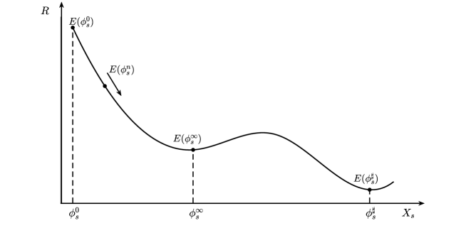
Figure 1: The accelerated momentum-based strategy.

The gradient descent approach is rooted in the dissipative PDE theory, where the energy functional as the free energy of the gradient flow model decays along a ”smooth” path or trajectory. In practical numerical implementations, for various treatments of $\nabla E(\Phi_{S}(t))$ in Eq. (3), $\nabla E(\Phi_{S}(t))$ may depend on state $\Phi_{S}(t)$ approximated at different time levels. As the result, the gradient-flow equations discretized with respect to pseudotime t may no longer be in the form of a discrete gradient flow of the energy functional. So, the resulting methods typically do not preserve the gradient-flow structure at the discrete level. This indicates that the structure-preserving strategy for the gradient flow discretization is not important for developing iterative numerical schemes for the minimization. Another potential drawback of such an approach is that solutions of the gradient flow model are in general critical points of the free energy, but are not necessarily minima (i.e., they can be saddle points). From this observation, we notice that preserving the gradient flow structure is secondary in designing an iterative optimization algorithm for the free energy. Several algorithms for the constrained optimization on Riemannian manifolds have been developed, in which constrained analogues of gradient, conjugate gradient and Newton’s algorithms are derived [1, 37]. These provide alternative approaches for us to follow in this study. Motivated by these developments, we will employ a perturbed, preconditioned, nonlinear conjugate gradient method (PPNCG) on the manifold $\mathcal{S}$ that guarantees the $L_{2}$ norm constraint for the solution of the nonlocal GP equation.

We note that vortex steady states of the coupled GP model often exhibit fine spatial structures, imposing strong requirements on the spatial discretization of the PDE system. To retain the required spatial resolution near the fine structures, we adopt the highly accurate Legendre-Galerkin spectral method [57] to discretize the PDE system in space. In time, we develop two strategies, one is in the accelerated momentum method, called ASGF method, and the other in the projected conjugate gradient method, called PPNCG method. The ASGF strategy hinges on a stabilizer corresponding to a nonlocal inertia ”regularization” of the over-damped normalized gradient flow model. This momentum-based method mitigates the strong local-minima attractive nature of the over-damped gradient flow to facilitate convergence to global minima. In the PPNCG method, we implement a perturbation strategy in the projected conjugate gradient method to avoid saddle points during minimization of the nonconvex Hamiltonian effectively. The algorithms resulted from both approaches are compared with the existing GFLM method extensively. The numerical results show that new methods perform better than the GFLM method while the PPNCG method outperforms the ASGF method, providing two efficient numerical solvers for solving the steady, coupled, nonlocal GP equations. It is worth noting that the new algorithms not only work well for the nonlocal GP systems, but also efficient for the simpler local GP equations.

In addition to the algorithms we present in this paper, we also devised other algorithms based on several selected high order time discretizations of the spatially, semi-discretized gradient flow systems. These algorithms include algorithms derived from applying second order time discretization, explicit and implicit 4th order Runge-Kutta discretization. None of the resulting iterative schemes outperforms the ASGF algorithm we present in this paper. This indicates that higher order temporal schemes applied to the normalized gradient flow does not necessarily yield better iterative schemes for steady states of the GP equations.

The rest of this paper is organized as follows. In §2, we present two new algorithms for a simplified GP model in the case of single-component BECs, detailing the temporal and spatial discretization strategies, and compare the new methods with the existing GFLM method. In §3, we extend the methods to the coupled GP model for binary BECs interacting with microwaves and compare their performance when computing symmetric and central vortex states. Finally, we draw the conclusion in §4.

2 Numerical methods for the single-component nonlocal GP equation

We consider the dimensionless 2D self-trapped single-component nonlocal GP equation in the weak microwave detuning limit [55, 65] without the external potential:

$$i\frac{\partial\psi}{\partial t}=\left[-\frac{1}{2}\triangle-\beta|\psi|^{2}-\breve{H}|\psi|^{2}\right]\psi,\quad{\bf x}\in\mathbb{R}^{2},$$ (4)

subject to constraint

$$\int_{\mathbb{R}^{2}}|\psi({\bf x})|^{2}d{\bf x}=1,$$ (5)

where the magnetic field $\breve{H}$ satisfies the following Poisson equation:

$$-\triangle\breve{H}=\gamma|\psi|^{2}\quad{\bf x}\in\mathbb{R}^{2}.$$ (6)

We identify the Hamiltonian of the conservative system as follows:

$$E(\psi)=\int_{\mathbb{R}^{2}}\bigg{[}\frac{1}{2}|\nabla\psi|^{2}-\frac{\beta}{2}|\psi({\bf x})|^{4}-\frac{\breve{H}}{2}|\psi({\bf x})|^{4}\bigg{]}d{\bf x}.$$ (7)

To find the symmetric and central vortex steady state solution of (7), we seek the following solution ansatz in polar coordinate $(r,\theta)$:

$$\psi({\bf x})=e^{-iS\theta}\phi_{S}(r),$$ (8)

where $S\in\mathbb{Z}$ is called the winding number and $\phi_{S}(r)$ is a real-valued function of $r=\sqrt{x^{2}+y^{2}}$. Since the laplace operator is rotational invariant and function $|\psi({\bf x})|$ is radially symmetric, it follows from (6) that magnetic field $\breve{H}$ is radially symmetric, its governing Poisson equation reduces to

$$-\frac{1}{r}\frac{d}{dr}\big{(}r\frac{dH}{dr}\big{)}=\gamma|\phi_{S}|^{2},\quad r\in[0,\infty),$$ (9)

in the polar coordinate $(r,\theta)$. When $S=0$, the solution is call a symmetric state; while $S>0$, it is called a central vortex state. For this type of solutions, Hamiltonian (7) reduces to the following functional parameterized by winding number S:

$$E(\phi_{S})=\pi\int_{0}^{\infty}\bigg{[}\left(\left(\phi_{S}^{\prime}\right)^{2}+\frac{S^{2}}{r^{2}}\phi_{S}^{2}\right)-\beta\phi_{S}^{4}-H\phi_{S}^{2}\bigg{]}\ rdr,$$ (10)

subject to constraint

$$2\pi\int_{0}^{\infty}\phi_{S}^{2}(r)\ rdr=1.$$ (11)

Our objective in this study is to solve for $\Phi_{S}(r)$ from the nonlocal GP equation. We consider solution $\phi_{S}(r)$ in the following function space:

$$X_{S}(\mathbb{R^{+}}):=H^{1}_{S}(\mathbb{R^{+}})\cap L^{4}_{S}(\mathbb{R^{+}})\cap L^{2}_{log,S}(\mathbb{R^{+}}),$$ (12)

whose various norms are defined as follows:

$$\|u\|_{L^{m}_{S}(\mathbb{R^{+}})}:=\big{(}2\pi\int_{0}^{+\infty}|u(r)|^{m}rdr\big{)}^{1/m},\quad m>0,$$

$$|u|_{H^{1}_{S}(\mathbb{R^{+}})}:=\bigg{(}2\pi\int_{0}^{+\infty}\big{(}|u^{\prime}(r)|^{2}+\frac{S^{2}}{r^{2}}|u(r)|^{2}\big{)}rdr\bigg{)}^{1/2},$$

$$\|u\|_{H^{1}_{S}(\mathbb{R^{+}})}:=\bigg{(}2\pi\int_{0}^{+\infty}\big{(}|u^{\prime}(r)|^{2}+(\frac{S^{2}}{r^{2}}+1)|u(r)|^{2}\big{)}rdr\bigg{)}^{1/2},$$

and

$$\|u\|_{L^{2}_{log,S}(\mathbb{R^{+}})}:=\big{(}2\pi\int_{0}^{+\infty}\ln(1+r)|u(r)|^{2}rdr\big{)}^{1/2}.$$

For a given $S$, we denote the symmetric state $\phi_{S}(r)$ at $S=0$ as $\phi_{S}^{s}$ and central vortex state when $S>0$ as $\phi_{S}^{c}$, respectively, both of which minimize $E(\phi_{S})$ at respective values of $S$ confined to manifold

$$\mathcal{S}_{1}:=\left\{\phi_{S}\ \big{|}\ \|\phi_{S}\|_{L^{2}(\mathbb{R}^{+})}^{2}=2\pi\int_{0}^{\infty}\phi_{S}^{2}(r)\ rdr=1,E(\phi_{S})<\infty\right\}.$$ (13)

The Euler-Lagrange equation when minimizing (10) over (11) is given by

$$\mu\phi_{S} =\frac{1}{2}\frac{\delta E(\phi_{S})}{\delta\phi_{S}}=-\frac{1}{2}\triangle_{r,S}\phi_{S}-\beta\phi_{S}^{2}\phi_{S}-H\phi_{S},$$ (14)

where

$$\triangle_{r,S}\triangleq\partial_{r}^{2}+\frac{1}{r}\partial_{r}-\frac{S^{2}}{r^{2}},$$ (15)

and $\mu$ serves as a Lagrange multiplier or nonlinear eigenvalue, which is given by constant

$$\mu(\phi_{S})=2\pi\int_{0}^{\infty}\bigg{[}\frac{1}{2}\left(\left(\phi_{S}^{\prime}\right)^{2}+\frac{S^{2}}{r^{2}}\phi_{S}^{2}\right)-\beta\phi_{S}^{4}-H\phi_{S}^{2}\bigg{]}\ rdr,$$ (16)

following (11).

Lemma 2.1.

(see [65]) There exists a symmetric state $(S=0)$ and a central vortex state $(S>0)$ of (10) when $\beta<\beta_{b}^{1}$, where $\beta_{b}^{1}$ is listed in Table 1.

$\mathrm{S}$	0	1	2	3	4	5	6	7
$\beta_{b}^{1}$	5.85	24.16	44.88	66.21	87.75	109.38	131.06	152.76
$\mathrm{S}$	8	9	10	11	12	13	14	15
$\beta_{b}^{1}$	174.47	196.20	217.94	239.68	261.42	283.17	304.92	326.67

Table 1: $\beta_{b}^{1}$ vs $S$.

When $\beta>\beta_{b}^{1}$, there does not exist any symmetric or central vortex state.

By Agmon’s Theorem (see [4]), it is easy to deduce that

$$\phi_{S}(r)=o(e^{-\alpha r})\quad\text{as $r\rightarrow\infty$ for every $\alpha>0$.}$$ (17)

Hence it’s reasonable to truncate the full domain $\mathbb{R}^{+}$ to the finite domain $U\triangleq[0,R]$ when solving the Euler-Lagrange equation numerically, where $R$ is a sufficiently large positive number. The boundary condition of the solution is given by $\phi_{S}(R)=0$, together with either $\phi_{S}(0)=0$ for $S>0$ or $\frac{d}{dr}\phi_{S}(0)=0$ for $S=0$.

Remark 2.1.

We note that pole condition $\frac{d}{dr}\phi_{S}(0)=0$ for $S=0$, derived from the parity argument is, however, not part of the essential pole condition for (14) [25, 39, 57]. Although in most cases there is no harm to impose this extra pole condition, we choose not to do so in our spectral representation since its implementation is more complicated and it may fail to give accurate results in some extreme (but still legitimate) cases.

In this case, Eq. (9) for the magnetic field $H$ reduces to

$$-\frac{1}{r}\frac{d}{dr}\big{(}r\frac{dH}{dr}\big{)}=\gamma|\phi_{S}|^{2},\quad r\in[0,R],$$ (18)

subject to a Robin boundary condition at $r=R$ [49, 65]:

$$\frac{dH}{dr}\bigg{|}_{r=R}=\frac{H(R)}{Rln(R)}.$$ (19)

Next, we present the first numerical method for solving the constrained minimization problem, called the accelerated, stabilizer-based normalized gradient flow method with Lagrange multipliers (ASGF).

2.1 Accelerated, stabilized normalized gradient flow (ASGF) method

We treat the minimization problem for the steady state over manifold $\mathcal{S}_{1}$ as a steady state solution of a gradient flow with the Hamiltonian as the free energy of the relaxation dynamics defined in the manifold, i.e.,

$$\partial_{t}\phi_{S}=-\frac{1}{2}\frac{\delta E}{\delta\phi_{S}},\quad\phi_{S}\in\mathcal{S}_{1},$$ (20)

where $\phi_{S}({\bf x},t)$ is treated as a pseudo-time (t) dependent function. We divide time interval $[0,\infty)$, using time step $\tau>0$, into $[t_{n},t_{n+1}]$, where $t_{n}=n\tau$ for $n=0,1,\cdots,\infty$. To deal with the confinement in the manifold, a simple projection step is implemented at the end of each interval. This method is known as the gradient flow with discrete normalization (GFDN) method [13], in which the corresponding PDE and the end-point projection are given as follows

$$\begin{split}&\partial_{t}\phi_{S}=-\frac{1}{2}\frac{\delta E(\phi_{S})}{\delta\phi_{S}}=\frac{1}{2}\triangle_{r,S}\phi_{S}+\big{(}\beta\phi_{S}^{2}+H\big{)}\phi_{S},\quad t_{n}<t<t_{n+1},\quad n\geq 0,\\ &\phi_{S}\left(r,t_{n+1}\right)\triangleq\phi_{S}\left(r,t_{n+1}^{+}\right)=\frac{\phi_{S}\left(r,t_{n+1}^{-}\right)}{\left\|\phi_{S}\left(r,t_{n+1}^{-}\right)\right\|_{L^{2}(\mathbb{R}^{+})}},\quad n\geq 0,\\ &\phi_{S}\left(r,0\right)=\phi_{S}^{0}(r),\quad\text{with}\quad\|\phi_{S}^{0}\|^{2}_{L^{2}(\mathbb{R}^{+})}=1,\end{split}$$ (21)

where $\phi_{S}\left(r,t_{n}^{\pm}\right)=\lim_{t\rightarrow t_{n}^{\pm}}\phi_{S}\left(r,t\right)$, and $\phi_{S}^{0}(r)$ is an initial guess for the symmetric or central vortex state solution.

GFDN (21) can be viewed as the first-order splitting method for the following continuous normalized gradient flow (CNGF) method [13]:

$$\begin{split}&\partial_{t}\phi_{S}=\frac{1}{2}\triangle_{r,S}\phi_{S}+\big{(}\beta\phi_{S}^{2}+H\big{)}\phi_{S}+\mu_{\phi_{S}}(t)\phi_{S},\quad t_{n}<t<t_{n+1},\quad n\geq 0,\\ &\phi_{S}\left(r,0\right)=\phi_{S}^{0}(r),\quad\text{with}\quad\|\phi_{S}^{0}\|^{2}_{L^{2}(\mathbb{R}^{+})}=1,\end{split}$$ (22)

where

$$\mu_{\phi_{S}}(t)=\frac{2\pi}{\left\|\phi_{S}\left(\cdot,t\right)\right\|_{L^{2}(\mathbb{R}^{+})}^{2}}\int_{0}^{\infty}\bigg{[}\frac{1}{2}\left(\left(\phi_{S}^{\prime}\right)^{2}+\frac{S^{2}}{r^{2}}\phi_{S}^{2}\right)-\beta\phi_{S}^{4}-H\phi_{S}^{2}\bigg{]}\ rdr.$$ (23)

It is proved that CNGF (22) is normalization-conservative and energy-diminishing [13].

To improve the GFDN approach to avoiding converging to a ”wrong” steady state solution [47] and to using a global strategy for the numerical computation of the local minima, we devise the following accelerated, stabilizer-based normalized gradient flow algorithm with Lagrange multipliers (ASGF) to compute the symmetric and central vortex state numerically. We add a nonlocal inertia term and modify the relaxation time in the GFDN model in (21) as follows

$$\begin{split}&\bigg{(}\alpha_{0}+\big{(}\alpha_{1}-\alpha_{2}\triangle_{r,S}\big{)}\partial_{t}\bigg{)}\partial_{t}\phi_{S}=\frac{1}{2}\triangle_{r,S}\phi_{S}+\big{(}\beta\phi_{S}^{2}+H\big{)}\phi_{S}+\mu_{\phi_{S}}(t_{n})\phi_{S}(r,t_{n}),\quad t_{n}<t<t_{n+1},\quad n\geq 0,\\ &\phi_{S}\left(r,t_{n+1}\right)\triangleq\phi_{S}\left(r,t_{n+1}^{+}\right)=\frac{\phi_{S}\left(r,t_{n+1}^{-}\right)}{\left\|\phi_{S}\left(r,t_{n+1}^{-}\right)\right\|_{L^{2}(\mathbb{R}^{+})}},\quad n\geq 0,\\ &\phi_{S}\left(r,0\right)=\phi_{S}^{0}(r),\quad\text{with}\quad\|\phi_{S}^{0}\|^{2}_{L^{2}(\mathbb{R}^{+})}=1,\end{split}$$ (24)

where the inertia

$$\alpha_{0}+\big{(}\alpha_{1}-\alpha_{2}\triangle_{r,S}\big{)}\partial_{t},\quad\alpha_{0},\alpha_{1},\alpha_{2}\geq 0,$$ (25)

serves as a stabilizer, and

$$\mu_{\phi_{S}}(t_{n})=\mu\big{(}\phi_{S}(\cdot,t_{n})\big{)}=2\pi\int_{0}^{\infty}\bigg{[}\frac{1}{2}\left(\left(\phi_{S}^{\prime}(r,t_{n})\right)^{2}+\frac{S^{2}}{r^{2}}\phi_{S}^{2}(r,t_{n})\right)-\beta\phi_{S}^{4}(r,t_{n})-H(r,t_{n})\phi_{S}^{2}(r,t_{n})\bigg{]}\ rdr.$$ (26)

Remark 2.2.

When $\alpha_{0}=1,\alpha_{1}=\alpha_{2}=0$, this is exactly the GFLM method used in [47]. Considering the following continuous Fourier wave in the polar coordinate

$$\phi_{S}(r,\theta,t)=e^{i(k_{x}\cdot rcos\theta+k_{y}\cdot rsin\theta+\omega t)},\quad\vec{k}=(k_{x},k_{y})^{T},$$ (27)

and plugging it into the linear part $\bigg{(}\alpha_{0}+\big{(}\alpha_{1}-\alpha_{2}\triangle_{r,\theta}\big{)}\partial_{t}\bigg{)}\partial_{t}\phi_{S}=\frac{1}{2}\triangle_{r,\theta}\phi_{S}$, where $\triangle_{r,\theta}\triangleq\partial_{r}^{2}+\frac{1}{r}\partial_{r}+\frac{1}{r^{2}}\partial_{\theta}^{2}$, we have

$$\omega=\frac{i\alpha_{0}\pm\sqrt{-\alpha_{0}^{2}+2|\vec{k}|^{2}\cdot\big{(}\alpha_{1}+\alpha_{2}|\vec{k}|^{2}\big{)}}}{2\big{(}\alpha_{1}+\alpha_{2}|\vec{k}|^{2}\big{)}},$$ (28)

from which we can see a smaller value of $\alpha_{0}$ combined with larger values of $\alpha_{1}$ and $\alpha_{2}$ leads to weakened damping of oscillations of the inertia-augmented system.

Denote $\dot{\phi}_{S}\triangleq\partial_{t}\phi_{S}$. Eq. (24) can be rewritten as the following gradient flow system

$$\begin{split}&\partial_{t}\phi_{S}=\dot{\phi}_{S},\\ &\bigg{(}\alpha_{0}+\big{(}\alpha_{1}-\alpha_{2}\triangle_{r,S}\big{)}\partial_{t}\bigg{)}\dot{\phi}_{S}=\frac{1}{2}\triangle_{r,S}\phi_{S}+\big{(}\beta\phi_{S}^{2}+H\big{)}\phi_{S}+\mu_{\phi_{S}}(t_{n})\phi_{S}(r,t_{n}),\\ &\phi_{S}\left(r,t_{n+1}\right)\triangleq\phi_{S}\left(r,t_{n+1}^{+}\right)=\frac{\phi_{S}\left(r,t_{n+1}^{-}\right)}{\left\|\phi_{S}\left(r,t_{n+1}^{-}\right)\right\|_{L^{2}(\mathbb{R}^{+})}},\quad n\geq 0,\\ &\phi_{S}\left(r,0\right)=\phi_{S}^{0}(r),\quad\text{with}\quad\|\phi_{S}^{0}\|^{2}_{L^{2}(\mathbb{R}^{+})}=1,\quad\text{and}\quad\dot{\phi}_{S}\left(r,0\right)=\dot{\phi}_{S}^{0}(r).\end{split}$$ (29)

2.1.1 Spatial discretization

We map $[0,R]$ into $[-1,1]$ using transformation $r=\frac{R}{2}(x+1)$, where $x\in I\triangleq[-1,1]$ and denote $u(x)=\phi_{S}(\frac{R}{2}(x+1))$, $v(x)=\dot{\phi}_{S}(\frac{R}{2}(x+1))$, and $\tilde{H}(x)=H(r)$. We use the Legendre-Galerkin method in $x\in[-1,1]$. Then, (29) is rewritten into the following for $x\in[-1,1]$:

$$\begin{split}&\partial_{t}u=v,\quad t_{n}<t<t_{n+1},\quad n\geq 0,\\ &\bigg{(}\alpha_{0}+\big{(}\alpha_{1}-\frac{4\alpha_{2}}{R^{2}}\triangle_{x,S}\big{)}\partial_{t}\bigg{)}v=\frac{2}{R^{2}}\triangle_{x,S}u+\big{(}\beta u^{2}+\tilde{H}\big{)}u+\mu\big{(}u(t_{n})\big{)}u(t_{n}),\quad t_{n}<t<t_{n+1},\quad n\geq 0,\\ &u(x,t_{n+1})\triangleq\frac{u(x,t^{+}_{n+1})}{\|u(x,t^{+}_{n+1})\|_{L^{2}(I)}},\quad n\geq 0,\\ &u^{0}(x)=\phi_{S}^{0}(r),\quad v^{0}(x)=\dot{\phi}_{S}^{0}(r),\end{split}$$ (30)

where $\|f\|^{2}_{L^{2}(I)}=\frac{\pi R^{2}}{2}\int_{-1}^{1}f^{2}(x)(x+1)dx$, and

$$\triangle_{x,S}\triangleq\partial_{x}^{2}+\frac{1}{x+1}\partial_{x}-\frac{S^{2}}{(x+1)^{2}}.$$ (31)

Now, chemical potential $\mu$ at time $t=t_{n}$ is rewritten into

$$\mu(u(t_{n}))= \pi\int_{-1}^{1}\bigg{[}\big{(}\partial_{x}u(t_{n})\big{)}^{2}+\frac{S^{2}}{(x+1)^{2}}u^{2}(t_{n})-\frac{R^{2}}{2}\big{(}\beta u^{2}(t_{n})+\tilde{H}(t_{n})\big{)}u^{2}(t_{n})\bigg{]}\ (x+1)dx$$ (32)

Given an integer N, we choose $P_{N}$ from the space of polynomials of degree less than or equal to N, and define

$$X_{N}(S)=\{u\in P_{N}:u(\pm 1)=0\}\quad\text{for}\quad S\neq 0,\quad X_{N}(0)=\{u\in P_{N}:u(1)=0\}.$$ (33)

Then, we consider the following Legendre-Galerkin approximation to Eq. (30), where the weight function (x+1) is the Jacobian of the polar transformation. We search for $(u_{N},v_{N})\in X_{N}(S)$ such that

$$\begin{split}&\int_{I}\partial_{t}u_{N}\cdot\omega(x+1)dx=\int_{I}v_{N}\cdot\omega(x+1)dx,\quad t_{n}<t<t_{n+1},\quad n\geq 0,\\ &\bigg{(}\alpha_{0}+\big{(}\alpha_{1}-\frac{4\alpha_{2}}{R^{2}}\triangle_{x,S}\big{)}\partial_{t}\bigg{)}v_{N}\cdot\omega(x+1)dx\\ &=\int_{I}\frac{2}{R^{2}}\triangle_{x,S}u_{N}\cdot\omega(x+1)dx+\int_{I}I_{N}g(u)\cdot\omega(x+1)dx+\mu(u_{N}(t_{n}))\int_{I}u_{N}(t_{n})\cdot\omega(x+1)dx,\\ &t_{n}<t<t_{n+1},\quad n\geq 0,\\ &u_{N}(t_{n+1})\triangleq\frac{u_{N}(t^{+}_{n+1})}{\|u_{N}(t^{+}_{n+1})\|_{L^{2}(I)}},\quad n\geq 0,\quad\forall\omega\in X_{N}(S),\end{split}$$ (34)

where $g(u)=\big{(}\beta u^{2}+\tilde{H}\big{)}u$ and $I_{N}f$ is the interpolation of $f$ in $\mathbb{P}_{N}$ at Legendre-Gauss-Lobotta collocation points.

To make the solution satisfying the boundary condition when $S\neq 0$, we construct the following function space:

$$X_{N}(S)=span\{\chi_{i}(x)=L_{i}(x)-L_{i+2}(x),\quad i=0,\cdots,N-2\},$$ (35)

where $L_{i}(x)$ is the $i$ th degree Legendre polynomial. We define

$$\begin{split}&a_{ij}=\int_{I}\chi_{j}^{\prime}\chi_{i}^{\prime}(x+1)dx,\quad A=\left(a_{ij}\right)_{i,j=0,1,\ldots,N-2},\\ &b_{ij}=\int_{I}\frac{1}{x+1}\chi_{j}\chi_{i}dx,\quad B=\left(B_{ij}\right)_{i,j=0,1,\ldots,N-2},\\ &c_{ij}=\int_{I}\chi_{j}\chi_{i}(x+1)dx,\quad C=\left(C_{ij}\right)_{i,j=0,1,\ldots,N-2},\\ &u_{N}=\sum_{i=0}^{N-2}\hat{u}_{i}\chi_{i}(x),\quad\vec{\hat{u}}=(\hat{u}_{0},\cdots,\hat{u}_{N-2})^{T},\\ &v_{N}=\sum_{i=0}^{N-2}\hat{v}_{i}\chi_{i}(x),\quad\vec{\hat{v}}=(\hat{v}_{0},\cdots,\hat{v}_{N-2})^{T}\\ &\big{(}I_{N}g(u)\big{)}(x)=\sum_{i=0}^{N-2}\hat{g}_{i}\chi_{i}(x),\quad\vec{\hat{g}}=(\hat{g}_{0},\cdots,\hat{g}_{N-2})^{T}.\end{split}$$ (36)

The following results follow from the orthogonality of the Legendre polynomials.

Lemma 2.2.

Matrix A and B are symmetric, tri-diagonal and given by

$$a_{ij}=\left\{\begin{array}[]{ll}2i+4,&j=i+1,\\ 4i+6,&j=i,\end{array}\quad b_{ij}=\left\{\begin{array}[]{ll}-\frac{2}{i+2},&j=i+1,\\ \frac{2(2i+3)}{(i+1)(i+2)},&j=i.\end{array}\right.\right.$$ (41)

Matrix C is symmetric and seven-diagonal with

$$c_{ij}=\left\{\begin{array}[]{ll}-\frac{2(i+3)}{(2i+5)(2i+7)},&j=i+3,\\ -\frac{2}{2i+5},&j=i+2,\\ \frac{2}{(2i+1)(2i+5)}+\frac{2(i+3)}{(2i+5)(2i+7)},&j=i+1,\\ \frac{2}{2i+1}+\frac{2}{2i+5},&j=i.\end{array}\right.$$ (46)

Eq. (34) with $\omega=\chi_{i}(x)$ reduces to

$$\begin{split}&\partial_{t}\vec{\hat{u}}=\vec{\hat{v}},\quad t_{n}<t<t_{n+1},\quad n\geq 0,\\ &\big{[}(\alpha_{0}+\alpha_{1}\partial_{t})C+\frac{4\alpha_{2}}{R^{2}}(A+S^{2}B)\partial_{t}\big{]}\vec{\hat{v}}=-\frac{2}{R^{2}}(A+S^{2}B)\vec{\hat{u}}+C\big{(}\vec{\hat{g}}+\mu(u_{N}^{n})\vec{\hat{u}}^{n}\big{)},\quad t_{n}<t<t_{n+1},\quad n\geq 0,\\ &u_{N}(t_{n+1})\triangleq\frac{u_{N}(t^{+}_{n+1})}{\|u_{N}(t^{+}_{n+1})\|_{L^{2}(I)}},\quad n\geq 0,\end{split}$$ (47)

In the case when $S=0$, we construct the following function space:

$$X_{N}(0)=span\{\chi_{i}(x)=L_{i}(x)-L_{i+1}(x),\quad i=0,\cdots,N-1\}.$$ (48)

Defining

$$\begin{split}&a_{ij}=\int_{I}\chi_{j}^{\prime}\chi_{i}^{\prime}(x+1)dx,\quad A=\left(a_{ij}\right)_{i,j=0,1,\ldots,N-1},\\ &c_{ij}=\int_{I}\chi_{j}\chi_{i}(x+1)dx,\quad C=\left(C_{ij}\right)_{i,j=0,1,\ldots,N-1},\\ &u_{N}=\sum_{i=0}^{N-1}\hat{u}_{i}\chi_{i}(x),\quad\vec{\hat{u}}=(\hat{u}_{0},\cdots,\hat{u}_{N-1})^{T},\\ &v_{N}=\sum_{i=0}^{N-1}\hat{v}_{i}\chi_{i}(x),\quad\vec{\hat{v}}=(\hat{v}_{0},\cdots,\hat{v}_{N-1})^{T},\\ &\big{(}I_{N}g(u)\big{)}(x)=\sum_{i=0}^{N-1}\hat{g}_{i}\chi_{i}(x),\quad\vec{\hat{g}}=(\hat{g}_{0},\cdots,\hat{g}_{N-1})^{T},\end{split}$$ (49)

one obtains the following results.

Lemma 2.3.

Matrix A is diagonal with

$$a_{ii}=2i+2.$$ (50)

Matrix C is symmetric and penta-diagonal with

$$c_{ij}=\left\{\begin{array}[]{ll}-\frac{2(i+2)}{(2i+3)(2i+5)},&j=i+2,\\ \frac{4}{(2i+1)(2i+3)(2i+5)},&j=i+1,\\ \frac{4(i+1)}{(2i+1)(2i+3)},&j=i.\end{array}\right.$$ (54)

Then, eq. (34) with $\omega=\chi_{i}(x)$ reduces to

$$\begin{split}&\partial_{t}\vec{\hat{u}}=\vec{\hat{v}},\quad t_{n}<t<t_{n+1},\quad n\geq 0,\\ &\big{[}(\alpha_{0}+\alpha_{1}\partial_{t})C+\frac{4\alpha_{2}}{R^{2}}A\partial_{t}\big{]}\vec{\hat{v}}=-\frac{2}{R^{2}}A\vec{\hat{u}}+C\big{(}\vec{\hat{g}}+\mu(u_{N}^{n})\vec{\hat{u}}^{n}\big{)},\quad t_{n}<t<t_{n+1},\quad n\geq 0,\\ &u_{N}(t_{n+1})\triangleq\frac{u_{N}(t^{+}_{n+1})}{\|u_{N}(t^{+}_{n+1})\|_{L^{2}(I)}},\quad n\geq 0.\end{split}$$ (55)

In the following, we address the issue of solving the transformed magnetic field $\tilde{H}$ equation by applying the Legendre-Galerkin method. In the transformed coordinate, eq. (18) with the boundary conditions is rewritten into

$$\begin{split}-\frac{4}{R^{2}}\big{(}\frac{d^{2}\tilde{H}}{dx^{2}}+\frac{1}{x+1}\frac{d\tilde{H}}{dx}\big{)}&=\gamma u^{2},\quad x\in[-1,1],\\ \frac{d\tilde{H}}{dx}\bigg{|}_{x=-1}&=0,\quad\frac{d\tilde{H}}{dx}\bigg{|}_{x=1}=\frac{\tilde{H}(1)}{2lnR}.\end{split}$$ (56)

We seek an approximation of $\tilde{H}$ in space

$$Y_{N}=\left\{\tilde{H}\in\mathbb{P}_{N}:\frac{d\tilde{H}}{dx}\bigg{|}_{x=-1}=0,\quad\frac{d\tilde{H}}{dx}\bigg{|}_{x=1}-\frac{\tilde{H}(1)}{2ln(R)}=0\right\}.$$ (57)

We define basis functions as follows

$$\zeta_{i}(x)=L_{i}(x)+a_{i}L_{i+1}(x)+b_{i}L_{i+2}(x),\quad i=0,1,\cdots,N-1,$$ (58)

where $a_{i}$ and $b_{i}$ are such that $\zeta_{i}(x)$ satisfies the boundary conditions of the function in $Y_{N}$.

Solving the linear algebra equations, we obtain

$$a_{i}=\frac{2i+3}{(i+2)^{2}\big{(}lnR(i+1)(i+3)-1\big{)}},\quad b_{i}=\frac{(i+1)^{2}}{(i+2)^{2}}\cdot\frac{lnR\cdot i(i+2)-1}{1-lnR(i+1)(i+3)},\quad i=0,1,\cdots,N-1.$$ (59)

The Legendre-Galerkin approximation to eq. (56) is equivalent to finding $\tilde{H}_{N}=\sum_{j=0}^{N-2}\hat{\tilde{H}}_{j}\zeta_{j}(x)\in Y_{N}$ such that

$$-\frac{4}{R^{2}}\sum_{j=0}^{N-2}\int_{-1}^{1}\big{(}\frac{d^{2}\zeta_{j}}{dx^{2}}+\frac{1}{x+1}\frac{d\zeta_{j}}{dx}\big{)}\zeta_{i}(x)(x+1)dx\hat{\tilde{H}}_{j}=\int_{-1}^{1}I_{N}(\gamma u^{2})\zeta_{i}(x)(x+1)dx.$$ (60)

Let

$$h_{i,j}=\int_{-1}^{1}\big{(}\frac{d^{2}\zeta_{j}}{dx^{2}}+\frac{1}{x+1}\frac{d\zeta_{j}}{dx}\big{)}\ \zeta_{i}(x)(x+1)dx,\quad H_{P}=\left(h_{ij}\right)_{i,j=0,1,\ldots,N-1}.$$ (61)

We have the following lemma.

Lemma 2.4.

Matrix $H_{P}$ is symmetric and tri-diagonal with

$$h_{ij}=\left\{\begin{array}[]{ll}2(i+4)a_{i},&j=i+1\\ 2(i+1)a_{i}+2(2i+3)b_{i}+2(i+2)a_{i}b_{i},&j=i\end{array}\right.$$ (64)

In the spectral representation of solutions, we define

$$\begin{split}&u_{N}^{n}=\sum_{i=0}^{N_{1}}\hat{u}_{i}^{n}\chi_{i}(x),\quad\vec{\hat{u}}^{n}=(\hat{u}_{0}^{n},\cdots,\hat{u}_{N_{1}}^{n})^{T},\quad u_{N}^{*}=\sum_{i=0}^{N_{1}}\hat{u}_{i}^{*}\chi_{i}(x),\quad\vec{\hat{u}}^{*}=(\hat{u}_{0}^{*},\cdots,\hat{u}_{N_{1}}^{*})^{T},\\ &v_{N}^{n}=\sum_{i=0}^{N_{1}}\hat{v}_{i}^{n}\chi_{i}(x),\quad\vec{\hat{v}}^{n}=(\hat{v}_{0}^{n},\cdots,\hat{v}_{N_{1}}^{n})^{T},\quad v_{N}^{*}=\sum_{i=0}^{N_{1}}\hat{v}_{i}^{*}\chi_{i}(x),\quad\vec{\hat{v}}^{*}=(\hat{v}_{0}^{*},\cdots,\hat{v}_{N_{1}}^{*})^{T},\\ &\big{(}I_{N}g(u^{n})\big{)}(x)=\sum_{i=0}^{N1}\hat{g}_{i}^{n}\chi_{i}(x),\quad\vec{\hat{g}}^{n}=(\hat{g}_{0}^{n},\cdots,\hat{g}_{N1}^{n})^{T},\\ &\text{with}\ N1=N-2\ \text{when}\ S\neq 0,\quad N1=N-1\ \text{when}\ S=0.\end{split}$$ (65)

2.1.2 Temporal discretization

After the Legendre-Galerkin approximation in space, we present two time-discredized schemes below. We use backward and forward mixed Euler scheme to discretize ODE system (47) for $S>0$ or (55) for $S=0$ in time to arrive at the first ASGF algorithm.

Algorithm 2.3 ($ASGF-I$).

Given initial data $u^{0},v^{0}$, compute the spectral coefficients $\vec{\hat{u}}^{0},\vec{\hat{v}}^{0}$. For $n>0$, compute $\vec{\hat{u}}^{n},\vec{\hat{v}}^{n}$ via

$$\begin{split}&\frac{\vec{\hat{u}}^{*}-\vec{\hat{u}}^{n}}{\triangle t}=\vec{\hat{v}}^{*},\quad t_{n}<t<t_{n+1},\quad n\geq 0,\\ &\alpha_{0}C\vec{\hat{v}}^{*}+\big{(}\alpha_{1}C+\frac{4\alpha_{2}}{R^{2}}(A+S^{2}B)\big{)}\frac{\vec{\hat{v}}^{*}-\vec{\hat{v}}^{n}}{\triangle t}=\big{(}-\frac{2}{R^{2}}(A+S^{2}B)-\alpha C\big{)}\vec{\hat{u}}^{*}+C\big{(}\alpha\vec{\hat{u}}^{n}+\vec{\hat{g}}^{n}+\mu(u_{N}^{n})\vec{\hat{u}}^{n}\big{)},\\ &\quad t_{n}<t<t_{n+1},\quad n\geq 0,\\ &u_{N}^{n+1}=\frac{u_{N}^{*}}{\|u_{N}^{*}\|_{L^{2}(I)}},\quad n\geq 0,\quad\forall S\geq 0,\end{split}$$ (66)

where $\alpha=max\{-\frac{1}{2}\big{(}\beta|u^{n}|^{2}+\tilde{H}^{n}+\mu(u^{n})\big{)},0\}$ is a chosen stabilization parameter such that the time step can be as large as possible;

until the $L_{2}$-norm of the residue is less than tolerance $\epsilon$.

In order to preserve the gradient-flow structure at the discrete level, different u-dependent terms on the right-hand side in the second expression of (47) and (55) should be approximated at the same time level, i.e., explicit treatment. Hence, we use the combined backward Euler method on the first equation of (47) or (55) and the forward Euler method on the second equation, we end up with the second scheme as follows.

Algorithm 2.4 ($ASGF-II$).

Given initial data $u^{0},v^{0}$, compute the spectral coefficients $\vec{\hat{u}}^{0},\vec{\hat{v}}^{0}$. For $n>0$, compute $\vec{\hat{u}}^{n},\vec{\hat{v}}^{n}$ via

$$\begin{split}&\frac{\vec{\hat{u}}^{*}-\vec{\hat{u}}^{n}}{\triangle t}=\vec{\hat{v}}^{*},\quad t_{n}<t<t_{n+1},\quad n\geq 0,\\ &\alpha_{0}C\vec{\hat{v}}^{*}+\big{(}\alpha_{1}C+\frac{4\alpha_{2}}{R^{2}}(A+S^{2}B)\big{)}\frac{\vec{\hat{v}}^{*}-\vec{\hat{v}}^{n}}{\triangle t}=-\frac{2}{R^{2}}(A+S^{2}B)\vec{\hat{u}}^{n}+C\big{(}\vec{\hat{g}}^{n}+\mu(u_{N}^{n})\vec{\hat{u}}^{n}\big{)},\\ &\quad t_{n}<t<t_{n+1},\quad n\geq 0,\\ &u_{N}^{n+1}=\frac{u_{N}^{*}}{\|u_{N}^{*}\|_{L^{2}(I)}},\quad n\geq 0,\quad\forall S\geq 0;\end{split}$$ (67)

until the $L_{2}$-norm of the residue is less than tolerance $\epsilon$.

Note that both schemes are first order in time. Next, we compare the new numerical schemes $ASGF-I$, $ASGF-II$ with the existing GFLM method, which is the special case of the above two schemes with $\alpha_{0}=1,\alpha_{1}=\alpha_{2}=0$, when solving central vortex state solutions.

2.1.3 Numerical results of the single-component GP model

The initial condition for the iterative scheme is chosen as $\phi_{S}^{0}(r)=\frac{1}{\sqrt{\pi S!}}r^{S}e^{-r^{2}/2}$ and $\dot{\phi}_{S}^{0}=0$. The stopping criterion for the time marching is that the $L^{2}$-norm of residue of the Euler–Lagrange equation (16) is less than given tolerance $\varepsilon=10^{-10}$. We take $S=2$, $\beta=30$, $\gamma=\pi$, $U=[0,20]$ with the dimension of the discrete Legendre space $N_{l}=200$. The performance of two methods with a few selected time step $\tau$ are tabulated in Table 2, where $E_{c}$ and $\mu_{c}$ are the energy and chemical potential at the central vortex state solution, respectively, and #$iter$ is the number of iterations (or time marching steps) used in computing the steady state. The time evolution of relative energy $E(\phi_{S}(\cdot,t))-E_{c}$ (in logarithmic scale) by the use of the two numerical schemes for computing the central vortex state solutions are shown in Figure 2.

From the numerical results obtained using the $ASGF-I$ scheme in Tab. 2 and Fig. 2, we observe that the computational time of the GFLM method, corresponding to $\alpha_{0}=1,\alpha_{1}=\alpha_{2}=0$, is much longer (about six times) than that of the ASGF method for the same time step, demonstrating that the $ASGF-I$ scheme is more efficient. Hence, $\alpha_{0}+\big{(}\alpha_{1}-\alpha_{2}\triangle_{r,S}\big{)}\partial_{t}$ indeed speeds up convergence to the steady state of the normalized gradient flow solution. Likewise, the $ASGF-II$ scheme outperforms the GFLM scheme considerably as well thanks to stabilizer $\alpha_{0}+\big{(}\alpha_{1}-\alpha_{2}\triangle_{r,S}\big{)}\partial_{t}$ again. We thus conclude that both ASGF schemes have better convergence properties than the GFLM scheme.

Scheme	$\tau$	$\alpha_{0}$	$\alpha_{1}$	$\alpha_{2}$	$\mathrm{CPU}(\mathrm{s})$	$E_{c}$	$\mu_{c}$	#$iter$
ASGF-I		1	0	0	323.5	0.4666956706	0.5688732593	32431
	0.01	0.0001	0.001	0.01	74.8	0.4666956706	0.5688732599	7199
		0.0001	0.001	0.005	50.1	0.4666956706	0.5688732599	4785
		1	0	0	37.5	0.4666956706	0.5688732593	3487
	0.1	0.001	0.01	0.05	7.8	0.4666956706	0.5688732599	711
		0.01	0.01	0.05	5.2	0.4666956706	0.5688732599	475
		1	0	0	6.60	0.4666956706	0.5688732594	590
	1	0.01	1	0.5	2.3	0.4666956706	0.5688732600	213
		0.03	1.2	0.5	1.9	0.4666956706	0.5688732600	168
ASGF-II		1	0	0	-	-	-	-
	0.01	1E-5	0.001	0.002	139.1	0.4666956706	0.5688732599	13448
		1E-6	0.001	0.0015	118.9	0.4666956706	0.5688732599	10889
		1	0	0	-	-	-	-
	0.1	0.001	0.01	0.05	88.9	0.4666956706	0.5688732598	8376
		0.0015	0.01	0.02	30.3	0.4666956706	0.5688732596	2873
		1	0	0	-	-	-	-
	1	0.015	1.2	0.8	21.2	0.4666956706	0.5688732596	2007
		0.015	1.1	0.5	18.5	0.4666956706	0.5688732600	1642

Table 2: Performance of the ASGF-I scheme and the II scheme when computing the central vortex state solution of a nonlocal single component GP model. The ASGF-I scheme outperforms the II scheme, and both are better than the GFLM scheme.

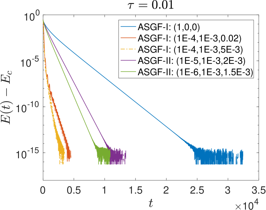
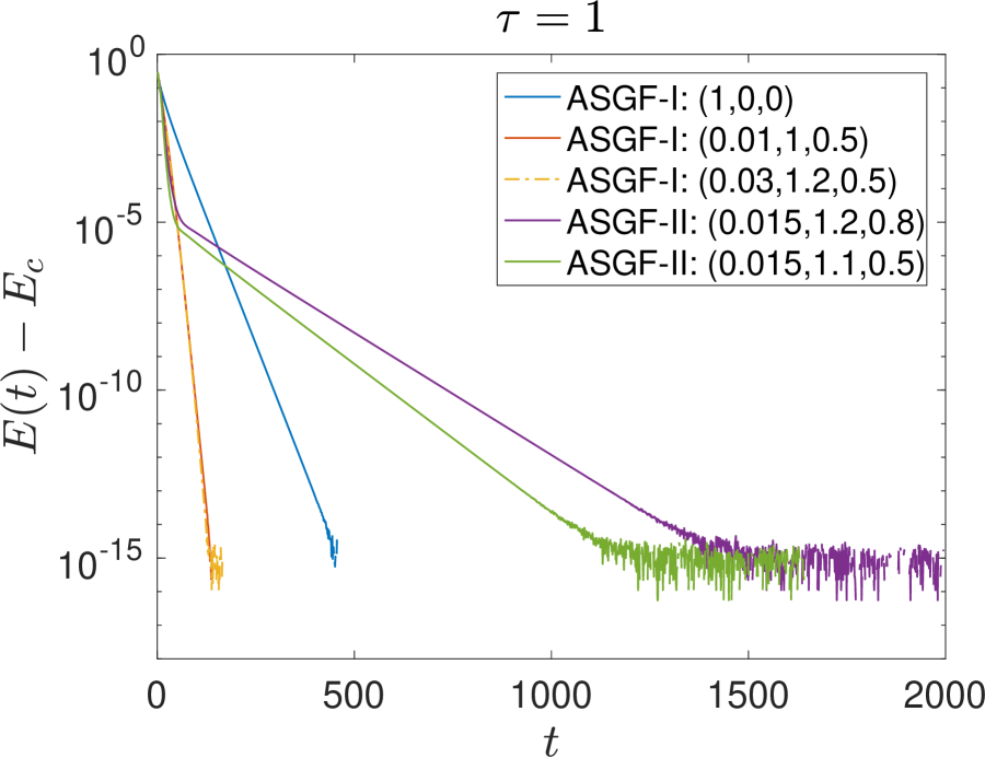
Figure 2: Time evolution of relative energy $E(\phi_{S}(\cdot,t))-E_{c}$ (in logarithmic scale) by different numerical schemes when computing the central vortex state solution. Left: $\tau=0.01$; Right: $\tau=1$. The triplet, for example $(1,0,0)$, in the inset represents $\alpha_{0}=1,\alpha_{1}=0,\alpha_{2}=0$, respectively.

Remark 2.5.

We have conducted additional numerical simulations for the rotating GP equation in a separate study, such as the logarithmic Schrödinger equation with the angular momentum, and noted the superior performance of the ASGF approach than that of GFLM. In fact, the GFLM scheme can only converge if time step $\triangle t$ is less than or equal to $\mathcal{O}(10^{-3})$ while the steady states can be reached with the ASGF scheme even at $\triangle t\thicksim\mathcal{O}(1)$.

2.2 Perturbed preconditioned nonlinear conjugate gradient (PPNCG) method

Here, we present a projection method which preserves the gradient-flow structure of (10) at the discrete level while implicitly accounting for the presence of the unit-norm constraint (11). The projected, preconditioned conjugate gradient method (PCG) for the minimization of $E(\phi_{S})$ on $\mathcal{S}_{1}$ is built on the update given by

$$\begin{split}\tilde{\phi_{S}}^{n+1}=\phi_{S}^{n}-\alpha_{n}P^{n}r^{n},\quad\phi_{S}^{n+1}=\frac{\tilde{\phi_{S}}^{n+1}}{\|\tilde{\phi_{S}}^{n+1}\|_{L^{2}(\mathbb{R}^{+})}},\end{split}$$ (68)

where

$$P^{n}:=\bigg{(}\pi\int_{0}^{\infty}\left(\left((\phi_{S}^{n})^{\prime}\right)^{2}+\frac{S^{2}}{r^{2}}(\phi_{S}^{n})^{2}\right)\ rdr-\frac{1}{2}\triangle_{r,S}\bigg{)}^{-1}$$ (69)

is the symmetric positive definite preconditioner, and

$$r^{n}:=-\frac{1}{2}\triangle_{r,S}\phi_{S}^{n}-\big{(}\beta(\phi_{S}^{n})^{2}+H^{n}\big{)}\phi_{S}^{n}-\mu_{n}\phi_{S}^{n}$$ (70)

is the residue.

We reformulate this update formula as follows

$$\phi_{S}^{n+1}=cos(\theta_{n})\phi_{S}^{n}+sin(\theta_{n})\frac{p^{n}}{\|p^{n}\|_{L^{2}(\mathbb{R}^{+})}},\quad p^{n}=d^{n}-\langle d^{n},\phi_{S}^{n}\rangle\phi_{S}^{n},$$ (71)

where $d^{n}=-P^{n}r^{n}+\beta_{n}d^{n-1}$ is the search direction, $\langle\cdot,\cdot\rangle$ is the $L^{2}(\mathbb{R}^{+})$ inner product and $\beta_{n}$ is the ”momentum” term chosen to enforce the conjugacy of search directions $d_{k},\ k=1,\cdots,n$. Either one of the following expressions

$$\begin{split}\beta_{n}=\beta_{n}^{FR}:=\frac{\langle r^{n},P^{n}r^{n}\rangle}{\langle r^{n-1},P^{n-1}r^{n-1}\rangle},\quad\text{(Fletcher–Reeves)},\\ \beta_{n}=\beta_{n}^{FR}:=max\left\{\frac{\langle r^{n}-r^{n-1},P^{n}r^{n}\rangle}{\langle r^{n-1},P^{n-1}r^{n-1}\rangle},0\right\},\quad\text{(Polak–Ribi\'{e}re))}\end{split}$$ (72)

can be used to update $\beta_{n}$. We note that equation (68) and (71) are equivalent when $\theta_{n}$ or $\alpha_{n}$ is small enough, with a one-to-one correspondence between $\theta_{n}$ and $\alpha_{n}$. In practice, $\theta_{n}$ may not be small, then a general line-minimization approach such as Brent’s algorithm should be adapted.

Expanding $\phi_{S}^{n+1}$ up to second-order in $\theta_{n}$, we obtain

$$\phi_{S}^{n+1}=\left(1-\frac{\theta_{n}^{2}}{2}\right)\phi_{S}^{n}+\theta_{n}\frac{p^{n}}{\left\|p^{n}\right\|}+\mathcal{O}\left(\theta_{n}^{3}\right)$$ (73)

and therefore

$$E\left(\phi_{S}^{n+1}\right)=E\left(\phi_{S}^{n}\right)+\frac{\theta_{n}}{\left\|p^{n}\right\|}\left\langle\nabla E\left(\phi_{S}^{n}\right),p^{n}\right\rangle+\frac{1}{2}\frac{\theta_{n}^{2}}{\left\|p^{n}\right\|^{2}}\left[\nabla^{2}E\left(\phi_{S}^{n}\right)\left[p^{n},p^{n}\right]-2\mu(\phi_{S}^{n})\left\|p^{n}\right\|^{2}\right]+\mathcal{O}\left(\theta_{n}^{3}\right).$$ (74)

Minimizing the above functional with respect to $\theta_{n}$ yields

$$\theta_{n}^{\mathrm{opt}}=\frac{-\left\langle\nabla E\left(\phi^{n}\right),p^{n}\right\rangle\left\|p^{n}\right\|}{\nabla^{2}E\left(\phi^{n}\right)\left[p^{n},p^{n}\right]-2\mu(\phi_{S}^{n})\left\|p_{n}\right\|^{2}}.$$ (75)

It’s known that the gradient descent method can be exponentially slow in the presence of saddle points [36]. Due to non-convexity of energy functional (10), its critical points may be an approximate saddle point instead of a local minimum. Then an appropriate procedure should be put in place to escape from the saddle point. We use the following perturbed preconditioned nonlinear conjugate gradient method (PPNCG) to find the minimum of the Hamiltonian confined in manifold $\mathcal{S}_{1}$ [8, 63].

Algorithm 2.6 (PPNCG ).

Initiate $\phi_{S}^{0}\in\mathcal{S}_{1}$ and use the steepest descent method in the first step.

$\mu_{0}=\mu(\phi_{S}^{0})$,

$r^{0}=-\frac{1}{2}\triangle_{r,S}\phi_{S}^{0}-\big{(}\beta(\phi_{S}^{0})^{2}+H^{0}\big{)}\phi_{S}^{0}-\mu_{0}\phi_{S}^{0}$,

$d^{0}=-P^{0}r^{0}$, $p^{0}=d^{0}-\langle d^{0},\phi_{S}^{0}\rangle\phi_{S}^{0}$,

$\theta_{0}=argmin_{\theta}E\big{(}cos(\theta)\phi_{S}^{0}+sin(\theta)\frac{p^{0}}{\|p^{0}\|_{L^{2}(\mathbb{R}^{+})}}\big{)}$,

$\phi_{S}^{1}=cos(\theta_{0})\phi_{S}^{0}+sin(\theta_{0})\frac{p^{0}}{\|p^{0}\|_{L^{2}(\mathbb{R}^{+})}}$,

Set $n=1,\|r^{1}\|=\|r^{0}\|$;

while $\|r^{n}\|\geq\varepsilon$ do

   Use the projected conjugate gradient method in this loop.

   $\mu_{n}=\mu(\phi_{S}^{n})$,

   $r^{n}=-\frac{1}{2}\triangle_{r,S}\phi_{S}^{n}-\big{(}\beta(\phi_{S}^{n})^{2}+H\big{)}\phi_{S}^{n}-\mu_{n}\phi_{S}^{n}$,

   $\beta_{n}=max\left\{\frac{\langle r^{n}-r^{n-1},P^{n}r^{n}\rangle}{\langle r^{n-1},P^{n-1}r^{n-1}\rangle},0\right\}$,

   $d^{n}=-P^{n}r^{n}+\beta_{n}d^{n-1}$,

   $p^{n}=d^{n}-\langle d^{n},\phi_{S}^{n}\rangle\phi_{S}^{n}$,

   $\theta_{n}=argmin_{\theta}E\big{(}cos(\theta)\phi_{S}^{n}+sin(\theta)\frac{p^{n}}{\|p^{n}\|_{L^{2}(\mathbb{R}^{+})}}\big{)}$,

   $\phi_{S}^{n+1}=cos(\theta_{n})\phi_{S}^{n}+sin(\theta_{n})\frac{p^{n}}{\|p^{n}\|_{L^{2}(\mathbb{R}^{+})}}$,

   $n=n+1$;

end while

Denote the above numerical solution by $\phi_{S}^{\star}$, perturb $\phi_{S}^{\star}$ by adding an appropriate level of noise in its tangent space and map it back to the manifold, denoted as $\phi_{S}^{\star,0}$, put the perturbed numerical solution $\phi_{S}^{\star,0}$ into above loop and run a few (about 7) iterations.

if the value of the energy functional decreases then

   it indicates that the numerical solution escapes from the approximate saddle point;

else

   if the value does not decrease then

      it is accepted as an approximate minimum.

   end if

end if

2.2.1 Numerical results of the single-component GP model

We compare the computational time and the number of iterations with a few selected values of $S$ and $\beta$ between the ASGF-I and PPNCG method when computing the symmetric state and central vortex state solution.

The initial condition is chosen as $\phi_{S}^{0}(r)=\frac{1}{\sqrt{\pi S!}}r^{S}e^{-r^{2}/2}$ and the initial velocity $\dot{\phi}_{S}^{0}=10\times\phi_{S}^{0}(r)$, time step $\tau=1$, $\alpha_{0}=0.01,\alpha_{1}=1,\alpha_{2}=0.2$ for ASGF-I. The stopping criterion for time marching is that the $L^{2}$-norm of residue of the Euler–Lagrange equation (16) is less than the given tolerance $\varepsilon=10^{-10}$. We take $R=18$ for $S=0$, $R=20$ for $S=2$, $R=30$ for $S=5$ and $R=35$ for $S=8$ with the dimension of the approximate solution space $N_{l}=10R$. The performance of the two methods are shown in Table 3, from which we see clearly that the PPNCG method is much better than the ASGF-I method.

S			0			2			5			8
$\beta$		0	3	4.5	0	30	40	0	50	80	0	100	140
ASGF-I	CPU(s)	1.61	1.48	2.12	2.12	2.48	10.25	12.33	12.99	64.32	24.51	110.72	447.98
	#$iter$	205	191	272	201	236	985	245	258	1303	274	1148	5104
PPNCG	CPU(s)	0.36	0.40	0.39	0.56	0.65	0.68	2.70	3.85	6.06	6.55	13.59	22.44
	#$iter$	28	32	31	30	39	40	40	56	77	46	95	158

Table 3: Performance comparison between the ASGF-I method and the PPNCG method in the total computational time and the number of iterations with respect to various values of $S$ and $\beta$.

3 Numerical methods for the coupled binary GP model

In this section, we extend the methods developed in §2 to the coupled binary GP model when computing the symmetric state and central vortex state solution. The coupled Gross-Pitaevskii equation with wave function $\Psi=(\psi_{\uparrow},\psi_{\downarrow})^{T}$ in a dimensionless 2D domain is given by

$$\begin{split}i\frac{\partial\psi_{\uparrow}}{\partial t}&=\big{[}-\frac{1}{2}\nabla^{2}+V_{\uparrow}({\bf x})-\eta-\beta|\psi_{\downarrow}|^{2}\big{]}\psi_{\uparrow}-\breve{H}\psi_{\downarrow},\\ i\frac{\partial\psi_{\downarrow}}{\partial t}&=\big{[}-\frac{1}{2}\nabla^{2}+V_{\downarrow}({\bf x})+\eta-\beta|\psi_{\uparrow}|^{2}\big{]}\psi_{\downarrow}-\overline{\breve{H}}\psi_{\uparrow},\end{split}$$ (76)

where $\overline{f}$ represents the conjugate of $f$, $\eta$ is the dimensionless detuning parameter, $\beta$ is the dimensionless contact interaction parameter, $V_{j}({\bf x})\ (j=1,2)$ are the external potentials, the magnetic field $\breve{H}$ satisfies

$$-\triangle\breve{H}=\gamma\psi_{\uparrow}({\bf x})\overline{\psi_{\downarrow}({\bf x})}.$$ (77)

If we use the fundamental solution of the 2D Poisson equation, $\breve{H}$ can be expressed explicitly by

$$\breve{H}=H_{0}+\breve{H_{1}}=H_{0}-\frac{\gamma}{2\pi}\int_{\mathbb{R}^{2}}\ln\left(\left|{\bf x}-{\bf x}^{\prime}\right|\right)\psi_{\uparrow}\left({\bf x}^{\prime}\right)\overline{\psi_{\downarrow}\left({\bf x}^{\prime}\right)}d{\bf x}^{\prime},$$ (78)

where $H_{0}$ is a background magnetic field and $\Delta H_{0}=0$.

The Hamiltonian of the conservative system is identified as

$$E(\Psi)= \int_{\mathbb{R}^{2}}\bigg{[}\sum_{j=\uparrow,\downarrow}\big{(}\frac{1}{2}|\nabla\psi_{j}|^{2}+V_{j}|\psi_{j}|^{2}\big{)}-\eta\big{(}|\psi_{\uparrow}|^{2}-|\psi_{\downarrow}|^{2}\big{)}-\beta|\psi_{\uparrow}|^{2}|\psi_{\downarrow}|^{2}$$

$$-2H_{0}Re{(\psi_{\uparrow}\overline{\psi_{\downarrow}})}-\frac{1}{\gamma}|\nabla\breve{H_{1}}|^{2}\bigg{]}d{\bf x}.$$ (79)

In the following, we assume external potentials $V_{1}=V_{\uparrow}$ and $V_{2}=V_{\downarrow}$ are radially symmetric, and we limit our search for the steady state of (3) to the central vortex form in polar coordinates $(r,\theta)$ as follows

$$\psi_{\uparrow}({\bf x})=e^{-iS\theta}\phi_{1}(r),\quad\psi_{\downarrow}({\bf x})=e^{-iS\theta}\phi_{2}(r),$$ (80)

where S is the winding number and $\Phi_{S}:=(\phi_{1},\phi_{2})^{T}$ is a real-valued radial wave function vector. The radial steady magnetic field $\breve{H}_{1}$ can then be expressed as:

$$-\frac{1}{r}\frac{d}{dr}\big{(}r\frac{dH_{1}}{dr}\big{)}=\gamma\phi_{1}\phi_{2},\quad r\in[0,\infty),$$ (81)

The corresponding energy functional (3) with the radially symmetric solution reduces to the following, parameterized by winding number S:

$$E(\Phi_{S})= 2\pi\int_{0}^{\infty}\big{[}\sum_{j=1,2}\frac{1}{2}\left(\left(\phi_{j}^{\prime}\right)^{2}+\frac{S^{2}}{r^{2}}\phi_{j}^{2}\right)+\sum_{j=1,2}V_{j}\phi_{j}^{2}$$

$$-\eta\big{(}\phi_{1}^{2}-\phi_{2}^{2}\big{)}-\beta\phi_{1}^{2}\phi_{2}^{2}-(2H_{0}+H_{1})\phi_{1}\phi_{2}\big{]}rdr,$$ (82)

subject to constraint

$$2\pi\int_{0}^{\infty}\big{(}\phi_{1}^{2}(r)+\phi_{2}^{2}(r)\big{)}\ rdr=1.$$ (83)

For a given winding number $S$, we denote the symmetric state as $\Phi_{S}^{s}$ at $S=0$ and central vortex state as $\Phi_{S}^{c}$ at $S>0$, respectively, which minimizes $E(\Phi_{S})$ in manifold

$$\mathcal{S}_{2}:=\left\{\Phi_{S}=\left(\phi_{1},\phi_{2}\right)^{T}\ \big{|}\ \|\Phi_{S}\|_{L^{2}(\mathbb{R}^{+})}^{2}=2\pi\int_{0}^{\infty}\big{(}\phi_{1}^{2}(r)+\phi_{2}^{2}(r)\big{)}\ rdr=1,E(\Phi_{S})<\infty\right\}.$$ (84)

One deduces the corresponding Euler-Lagrange equations of the constrained minimization problem as follows

$$\begin{split}\mu\phi_{1}&=-\frac{1}{2}\triangle_{r,S}\phi_{1}+\bigg{[}V_{1}-\eta-\beta\phi_{2}^{2}\bigg{]}\phi_{1}-\big{(}H_{0}+H_{1}\big{)}\phi_{2},\\ \mu\phi_{2}&=-\frac{1}{2}\triangle_{r,S}\phi_{2}+\bigg{[}V_{2}+\eta-\beta\phi_{1}^{2}\bigg{]}\phi_{2}-\big{(}H_{0}+H_{1}\big{)}\phi_{1}.\end{split}$$ (85)

The corresponding Lagrange multiplier or eigenvalue (chemical potential) is given by

$$\mu(\Phi_{S})= 2\pi\int_{0}^{\infty}\bigg{[}\sum_{j=1,2}\frac{1}{2}\left(\left(\phi_{j}^{\prime}\right)^{2}+\frac{S^{2}}{r^{2}}\phi_{j}^{2}\right)+\sum_{j=1,2}V_{j}\phi_{j}^{2}-\eta\big{(}\phi_{1}^{2}-\phi_{2}^{2}\big{)}-2\beta\phi_{1}^{2}\phi_{2}^{2}-2(H_{0}+H_{1})\phi_{1}\phi_{2}\bigg{]}\ rdr.$$ (86)

We search for steady state solutions in the function space defined by

$$X_{S}^{2}(\mathbb{R^{+}}):=H^{1}_{S}(\mathbb{R^{+}})\cap L^{4}_{S}(\mathbb{R^{+}})\cap L^{2}_{V}(\mathbb{R}^{+})\cap L_{log,S}^{2}(\mathbb{R}^{+}),$$ (87)

where $L^{2}_{V}(\mathbb{R}^{+}):=\left\{\Phi_{S}\bigg{|}\int_{0}^{\infty}(V_{1}(r)\phi_{1}^{2}(r)+V_{2}(r)\phi_{2}^{2}(r))rdr<\infty\right\}$, and $\lim\limits_{r\rightarrow+\infty}V_{j}(r)=+\infty(j=1,2)$.

Lemma 3.1.

(see [65]) In Hilbert space $X_{S}^{2}(\mathbb{R}^{+})$ and for any given $S\geq 0$, there exists a symmetric or central vortex steady state $\Phi_{S}=(\phi_{1},\phi_{2})^{T}$ of (3) when $\beta\leq\beta_{b}$ and $V_{j}(r)\geq\frac{\gamma}{8\pi}r^{2},j=1,2$, where $\beta_{b}$ is defined in Table 4. When $\beta>2\beta_{b}$, there does not exist any symmetric or central vortex steady state.

S	0	1	2	3	4	5	6	7
$\beta_{b}$	11.70	48.31	89.75	132.42	175.50	218.76	262.11	305.51
S	8	9	10	11	12	13	14	15
$\beta_{b}$	348.94	392.40	435.87	479.35	522.84	566.33	609.83	653.34

Table 4: $\beta_{b}$ vs S

3.1 ASGF method

The normalized gradient flow model for computing the symmetric and central vortex state of the nonlocal binary GP model reads as follows. Given the time sequence $t_{n}=n\tau$ for $n=0,1,2,\cdots$, for $t\in[t_{n},t_{n+1})(n\geq 0)$, one solves the following gradient flow model in time:

$$\begin{split}&\bigg{(}\alpha_{01}+\big{(}\alpha_{11}-\alpha_{21}\triangle_{r,S}\big{)}\partial_{t}\bigg{)}\partial_{t}\phi_{1}=\frac{1}{2}\triangle_{r,S}\phi_{1}-g_{1}+\mu(\Phi_{S}(t_{n}))\phi_{1}(r,t_{n}),\quad t_{n}<t<t_{n+1},\quad n\geq 0,\\ &\bigg{(}\alpha_{02}+\big{(}\alpha_{12}-\alpha_{22}\triangle_{r,S}\big{)}\partial_{t}\bigg{)}\partial_{t}\phi_{2}=\frac{1}{2}\triangle_{r,S}\phi_{2}-g_{2}+\mu(\Phi_{S}(t_{n}))\phi_{2}(r,t_{n}),\quad t_{n}<t<t_{n+1},\quad n\geq 0,\\ &\Phi_{S}\left(r,t_{n+1}\right)\triangleq\Phi_{S}\left(r,t_{n+1}^{+}\right)=\frac{\Phi_{S}\left(r,t_{n+1}^{-}\right)}{\left\|\Phi_{S}\left(r,t_{n+1}^{-}\right)\right\|_{L^{2}(\mathbb{R}^{+})}},\quad n\geq 0,\\ &\Phi_{S}\left(r,0\right)=\Phi_{S}^{0}(r),\quad\text{with}\quad\|\Phi_{S}^{0}\|^{2}_{L^{2}(\mathbb{R}^{+})}=1,\quad\dot{\Phi}_{S}\left(r,0\right)=\dot{\Phi}_{S}^{0}(r),\end{split}$$ (88)

where

$$\begin{split}g_{1}\triangleq\big{(}V_{1}-\eta-\beta\phi_{2}^{2}\big{)}\phi_{1}-\big{(}H_{0}+H_{1}\big{)}\phi_{2},\\ g_{2}\triangleq\big{(}V_{2}+\eta-\beta\phi_{1}^{2}\big{)}\phi_{2}-\big{(}H_{0}+H_{1}\big{)}\phi_{1}.\end{split}$$ (89)

Define $\dot{\phi}_{i}\triangleq\partial_{t}\phi_{i},\quad i=1,2$. Then the above system (88) can be rewritten into:

$$\begin{split}&\partial_{t}\phi_{1}=\dot{\phi}_{1},\\ &\bigg{(}\alpha_{01}+\big{(}\alpha_{11}-\alpha_{21}\triangle_{r,S}\big{)}\partial_{t}\bigg{)}\dot{\phi}_{1}=\frac{1}{2}\triangle_{r,S}\phi_{1}-g_{1}+\mu(\Phi_{S}(t_{n}))\phi_{1}(r,t_{n}),\quad t_{n}<t<t_{n+1},\quad n\geq 0,\\ &\partial_{t}\phi_{2}=\dot{\phi}_{2},\\ &\bigg{(}\alpha_{02}+\big{(}\alpha_{12}-\alpha_{22}\triangle_{r,S}\big{)}\partial_{t}\bigg{)}\dot{\phi}_{2}=\frac{1}{2}\triangle_{r,S}\phi_{2}-g_{2}+\mu(\Phi_{S}(t_{n}))\phi_{2}(r,t_{n}),\quad t_{n}<t<t_{n+1},\quad n\geq 0,\\ &\Phi_{S}\left(r,t_{n+1}\right)\triangleq\Phi_{S}\left(r,t_{n+1}^{+}\right)=\frac{\Phi_{S}\left(r,t_{n+1}^{-}\right)}{\left\|\Phi_{S}\left(r,t_{n+1}^{-}\right)\right\|_{L^{2}(\mathbb{R}^{+})}},\quad n\geq 0,\\ &\Phi_{S}\left(r,0\right)=\Phi_{S}^{0}(r),\quad\text{with}\quad\|\Phi_{S}^{0}\|^{2}_{L^{2}(\mathbb{R}^{+})}=1,\quad\dot{\Phi}_{S}\left(r,0\right)=\dot{\Phi}_{S}^{0}(r).\end{split}$$ (90)

In $\mathbb{R}^{+}$ with confining potential $V_{i}(r)(i.e.,lim_{r\rightarrow+\infty}V_{i}(r)=+\infty,i=1,2)$, we note that the symmetric and central vortex state solution decays exponentially fast as $r\rightarrow+\infty$ [26]. Hence, the unbounded domain $\mathbb{R}^{+}$ can be truncated into a sufficient large bounded interval $U=[0,R]$ when one solves for the steady state solution. We use the following coordinate transformation $r=\frac{R}{2}(x+1)$ to transform the equation into one defined in $x\in I\triangleq[-1,1]$ by setting $u_{i}(x)=\phi_{i}(\frac{R}{2}(x+1))$, $v_{i}(x)=\dot{\phi}_{i}(\frac{R}{2}(x+1)),i=1,2$, and $\tilde{H}_{1}(x)=H_{1}(r)$. The transformed equation system is given by

$$\begin{split}&\partial_{t}u_{1}=v_{1},\quad t_{n}<t<t_{n+1},\quad n\geq 0,\\ &\bigg{(}\alpha_{01}+\big{(}\alpha_{11}-\frac{4\alpha_{21}}{R^{2}}\triangle_{x,S}\big{)}\partial_{t}\bigg{)}v_{1}=\frac{2}{R^{2}}\triangle_{x,S}u_{1}-\tilde{g}_{1}+\mu(\Phi_{S}(t_{n}))u_{1}(t_{n}),\quad t_{n}<t<t_{n+1},\quad n\geq 0,\\ &\partial_{t}u_{2}=v_{2},\quad t_{n}<t<t_{n+1},\quad n\geq 0,\\ &\bigg{(}\alpha_{02}+\big{(}\alpha_{12}-\frac{4\alpha_{22}}{R^{2}}\triangle_{x,S}\big{)}\partial_{t}\bigg{)}v_{2}=\frac{2}{R^{2}}\triangle_{x,S}u_{2}-\tilde{g}_{2}+\mu(\Phi_{S}(t_{n}))u_{2}(t_{n}),\quad t_{n}<t<t_{n+1},\quad n\geq 0,\\ &\stackrel{{\scriptstyle\raisebox{-2.0pt}[0.0pt][0.0pt]{\small$\rightharpoonup$}}}{{u}}(t_{n+1})\triangleq\frac{\stackrel{{\scriptstyle\raisebox{-2.0pt}[0.0pt][0.0pt]{\small$\rightharpoonup$}}}{{u}}(t^{+}_{n+1})}{\|\stackrel{{\scriptstyle\raisebox{-2.0pt}[0.0pt][0.0pt]{\small$\rightharpoonup$}}}{{u}}(t^{+}_{n+1})\|_{L^{2}(I)}},\quad n\geq 0,\\ &\stackrel{{\scriptstyle\raisebox{-2.0pt}[0.0pt][0.0pt]{\small$\rightharpoonup$}}}{{u}}(x,0)=\Phi_{S}^{0}(r),\quad\text{with}\quad\|\stackrel{{\scriptstyle\raisebox{-2.0pt}[0.0pt][0.0pt]{\small$\rightharpoonup$}}}{{u}}^{0}\|^{2}_{L^{2}(I)}=1,\quad\stackrel{{\scriptstyle\raisebox{-2.0pt}[0.0pt][0.0pt]{\small$\rightharpoonup$}}}{{v}}(x,0)=\dot{\Phi}_{S}^{0}(r),\end{split}$$ (91)

where

$$\begin{split}\tilde{g}_{1}\triangleq\big{(}\tilde{V_{1}}-\eta-\beta u_{2}^{2}\big{)}u_{1}-\big{(}H_{0}+\tilde{H}_{1}\big{)}u_{2},\\ \tilde{g}_{2}\triangleq\big{(}\tilde{V_{2}}+\eta-\beta u_{1}^{2}\big{)}u_{2}+\big{(}H_{0}+\tilde{H}_{1}\big{)}u_{1},\end{split}$$ (92)

and $\|\stackrel{{\scriptstyle\raisebox{-2.0pt}[0.0pt][0.0pt]{\small$\rightharpoonup$}}}{{u}}(t^{+}_{n+1})\|^{2}_{L^{2}(I)}\triangleq\|u_{1}(t^{+}_{n+1})\|^{2}_{L^{2}(I)}+\|u_{2}(t^{+}_{n+1})\|^{2}_{L^{2}(I)}$. The chemical potential $\mu$ at time $t=t_{n}$ can be rewritten as

$$\mu(\Phi_{S}(t_{n}))= \sum_{i=1,2}\pi\int_{-1}^{1}\bigg{(}\big{(}\partial_{x}u_{i}(t_{n})\big{)}^{2}+\frac{S^{2}}{(x+1)^{2}}u_{i}^{2}(t_{n})\bigg{)}\ (x+1)dx$$

$$+\frac{\pi R^{2}}{2}\int_{-1}^{1}\bigg{(}\big{(}\tilde{V_{1}}-\eta-\beta u_{2}^{2}(t_{n})\big{)}u_{1}(t_{n})+\big{(}H_{0}+\tilde{H}_{1}(t_{n})\big{)}u_{2}(t_{n})\bigg{)}u_{1}(t_{n})\ (x+1)dx$$

$$+\frac{\pi R^{2}}{2}\int_{-1}^{1}\bigg{(}\big{(}\tilde{V_{2}}+\eta-\beta u_{1}(t_{n})^{2}\big{)}u_{2}(t_{n})+\big{(}H_{0}+\tilde{H}_{1}(t_{n})\big{)}u_{1}(t_{n})\bigg{)}u_{2}(t_{n})\ (x+1)dx.$$ (93)

Following the development for ASGF-I, we obtain the following decoupled discrete schemes.

Algorithm 3.1.

Given initial data $u_{i}^{0},v_{i}^{0}$, $i=1,2$, compute the spectral coefficients $\vec{\hat{u_{i}}}^{0},\vec{\hat{v_{i}}}^{0}$. For $n>0$, compute $\vec{\hat{u_{i}}}^{n},\vec{\hat{v_{i}}}^{n}$ via

$$\begin{split}&\frac{\vec{\hat{u}}_{1}^{*}-\vec{\hat{u}}_{1}^{n}}{\triangle t}=\vec{\hat{v}}_{1}^{*},\quad t_{n}<t<t_{n+1},\quad n\geq 0,\\ &\alpha_{01}C\vec{\hat{v}}_{1}^{*}+\big{(}\alpha_{11}C+\frac{4\alpha_{21}}{R^{2}}(A+S^{2}B)\big{)}\frac{\vec{\hat{v}}_{1}^{*}-\vec{\hat{v}}_{1}^{n}}{\triangle t}=\big{(}-\frac{2}{R^{2}}(A+S^{2}B)-\alpha_{1}C\big{)}\vec{\hat{u}}_{1}^{*}+C\big{(}\alpha_{1}\vec{\hat{u}}_{1}^{n}+\vec{\hat{g}}_{1}^{n}+\mu(u_{N}^{n})\vec{\hat{u}}_{1}^{n}\big{)},\\ &\frac{\vec{\hat{u}}_{2}^{*}-\vec{\hat{u}}_{2}^{n}}{\triangle t}=\vec{\hat{v}}_{2}^{*},\quad t_{n}<t<t_{n+1},\quad n\geq 0,\\ &\alpha_{02}C\vec{\hat{v}}_{2}^{*}+\big{(}\alpha_{12}C+\frac{4\alpha_{22}}{R^{2}}(A+S^{2}B)\big{)}\frac{\vec{\hat{v}}_{2}^{*}-\vec{\hat{v}}_{2}^{n}}{\triangle t}=\big{(}-\frac{2}{R^{2}}(A+S^{2}B)-\alpha_{2}C\big{)}\vec{\hat{u}}_{2}^{*}+C\big{(}\alpha_{2}\vec{\hat{u}}_{2}^{n}+\vec{\hat{g}}_{2}^{n}+\mu(u_{N}^{n})\vec{\hat{u}}_{2}^{n}\big{)},\\ &\quad t_{n}<t<t_{n+1},\quad n\geq 0,\\ &\stackrel{{\scriptstyle\raisebox{-2.0pt}[0.0pt][0.0pt]{\small$\rightharpoonup$}}}{{u}}_{N}^{n+1}=\frac{\stackrel{{\scriptstyle\raisebox{-2.0pt}[0.0pt][0.0pt]{\small$\rightharpoonup$}}}{{u}}_{N}^{*}}{\|\stackrel{{\scriptstyle\raisebox{-2.0pt}[0.0pt][0.0pt]{\small$\rightharpoonup$}}}{{u}}_{N}^{*}\|_{L^{2}(I)}},\quad n\geq 0,\quad\forall S\geq 0,\end{split}$$ (94)

where $\alpha_{1}=max\{\frac{1}{2}\big{(}\tilde{V_{1}}-\eta-\beta(u^{n}_{2})^{2}+|H_{0}+\tilde{H}_{1}^{n}|-\mu(u^{n})\big{)},0\}$ and $\alpha_{2}=max\{\frac{1}{2}\big{(}\tilde{V_{2}}+\eta-\beta(u^{n}_{1})^{2}+|H_{0}+\tilde{H}_{1}^{n}|-\mu(u^{n})\big{)},0\}$ are chosen stabilization parameters such that the time step can be as large as possible;

until the $L_{2}$-norm of the residue is less than tolerance $\epsilon$.

3.2 PPNCG method

Analogous to the development of numerical schemes for the single-component GP equation, we arrive at the PPNCG method for the binary GP system. The update in this method is defined by

$$\begin{split}\tilde{\Phi_{S}}^{n+1}&=\Phi_{S}^{n}-\alpha_{n}\ diag\left(P^{n},P^{n}\right)\ \stackrel{{\scriptstyle\raisebox{-2.0pt}[0.0pt][0.0pt]{\small$\rightharpoonup$}}}{{r}}^{n},\\ \Phi_{S}^{n+1}&=\frac{\tilde{\Phi_{S}}^{n+1}}{\|\tilde{\Phi_{S}}^{n+1}\|_{L^{2}(\mathbb{R}^{+})}},\end{split}$$ (95)

where

$$P^{n}:=\left(\pi\int_{0}^{\infty}\left(\left((\phi_{1}^{n})^{\prime}\right)^{2}+\frac{S^{2}}{r^{2}}(\phi_{1}^{n})^{2}+\left((\phi_{2}^{n})^{\prime}\right)^{2}+\frac{S^{2}}{r^{2}}(\phi_{2}^{n})^{2}\right)\ rdr-\frac{1}{2}\triangle_{r,S}\right)^{-1}$$ (96)

is the symmetric positive definite preconditioner, and

$$\stackrel{{\scriptstyle\raisebox{-2.0pt}[0.0pt][0.0pt]{\small$\rightharpoonup$}}}{{r}}^{n}=\left(\begin{array}[]{c}r_{1}^{n}\\ r_{2}^{n}\end{array}\right)\triangleq\left(\begin{array}[]{c}-\frac{1}{2}\triangle_{r,S}\phi_{1}^{n}+\bigg{[}V_{1}-\eta-\beta(\phi_{2}^{n})^{2}\bigg{]}\phi_{1}^{n}-\big{(}H_{0}+H_{1}^{n}\big{)}\phi_{2}^{n}-\mu^{n}\phi_{1}^{n}\\ -\frac{1}{2}\triangle_{r,S}\phi_{2}^{n}+\bigg{[}V_{2}+\eta-\beta(\phi_{1}^{n})^{2}\bigg{]}\phi_{2}^{n}-\big{(}H_{0}+H_{1}^{n}\big{)}\phi_{1}^{n}-\mu^{n}\phi_{2}^{n}\end{array}\right)$$ (101)

is the residue.

We reformulate this formula as follows

$$\Phi_{S}^{n+1}=cos(\theta_{n})\Phi_{S}^{n}+sin(\theta_{n})\frac{\stackrel{{\scriptstyle\raisebox{-2.0pt}[0.0pt][0.0pt]{\small$\rightharpoonup$}}}{{p}}^{n}}{\|\stackrel{{\scriptstyle\raisebox{-2.0pt}[0.0pt][0.0pt]{\small$\rightharpoonup$}}}{{p}}^{n}\|_{L^{2}(\mathbb{R}^{+})}},$$ (102)

with

$$\stackrel{{\scriptstyle\raisebox{-2.0pt}[0.0pt][0.0pt]{\small$\rightharpoonup$}}}{{p}}^{n}=\stackrel{{\scriptstyle\raisebox{-2.0pt}[0.0pt][0.0pt]{\small$\rightharpoonup$}}}{{d}}^{n}-\ \langle\stackrel{{\scriptstyle\raisebox{-2.0pt}[0.0pt][0.0pt]{\small$\rightharpoonup$}}}{{d}}^{n},\Phi_{S}^{n}\rangle\Phi_{S}^{n},$$ (103)

where $\stackrel{{\scriptstyle\raisebox{-2.0pt}[0.0pt][0.0pt]{\small$\rightharpoonup$}}}{{d}}^{n}=-diag\left(P^{n},P^{n}\right)\stackrel{{\scriptstyle\raisebox{-2.0pt}[0.0pt][0.0pt]{\small$\rightharpoonup$}}}{{r}}^{n}+\beta_{n}\stackrel{{\scriptstyle\raisebox{-2.0pt}[0.0pt][0.0pt]{\small$\rightharpoonup$}}}{{d}}^{n-1}$ is the search direction. Expanding $\Phi_{S}^{n+1}$ up to second-order in $\theta_{n}$, we obtain

$$\Phi_{S}^{n+1}=\left(1-\frac{\theta_{n}^{2}}{2}\right)\Phi_{S}^{n}+\theta_{n}\frac{\stackrel{{\scriptstyle\raisebox{-2.0pt}[0.0pt][0.0pt]{\small$\rightharpoonup$}}}{{p}}^{n}}{\|\stackrel{{\scriptstyle\raisebox{-2.0pt}[0.0pt][0.0pt]{\small$\rightharpoonup$}}}{{p}}^{n}\|_{L^{2}(\mathbb{R}^{+})}}+\mathcal{O}\left(\theta_{n}^{3}\right)$$ (104)

and

$$E\left(\Phi_{S}^{n+1}\right)=E\left(\Phi_{S}^{n}\right)+\frac{2\theta_{n}}{\|\stackrel{{\scriptstyle\raisebox{-2.0pt}[0.0pt][0.0pt]{\small$\rightharpoonup$}}}{{p}}^{n}\|}\left\langle\stackrel{{\scriptstyle\raisebox{-2.0pt}[0.0pt][0.0pt]{\small$\rightharpoonup$}}}{{r}}^{n},\stackrel{{\scriptstyle\raisebox{-2.0pt}[0.0pt][0.0pt]{\small$\rightharpoonup$}}}{{p}}^{n}\right\rangle+\frac{\theta_{n}^{2}}{\|\stackrel{{\scriptstyle\raisebox{-2.0pt}[0.0pt][0.0pt]{\small$\rightharpoonup$}}}{{p}}^{n}\|^{2}}\left[\frac{1}{2}\nabla^{2}E\left(\Phi_{S}^{n}\right)[\stackrel{{\scriptstyle\raisebox{-2.0pt}[0.0pt][0.0pt]{\small$\rightharpoonup$}}}{{p}}^{n},\stackrel{{\scriptstyle\raisebox{-2.0pt}[0.0pt][0.0pt]{\small$\rightharpoonup$}}}{{p}}^{n}]-\mu^{n}\|\stackrel{{\scriptstyle\raisebox{-2.0pt}[0.0pt][0.0pt]{\small$\rightharpoonup$}}}{{p}}^{n}\|^{2}\right]+\mathcal{O}\left(\theta_{n}^{3}\right).$$ (105)

Minimizing (105) with respect to $\theta_{n}$ yields

$$\theta_{n}=-\frac{\|\stackrel{{\scriptstyle\raisebox{-2.0pt}[0.0pt][0.0pt]{\small$\rightharpoonup$}}}{{p}}^{n}\|\cdot\left\langle\stackrel{{\scriptstyle\raisebox{-2.0pt}[0.0pt][0.0pt]{\small$\rightharpoonup$}}}{{r}}^{n},\stackrel{{\scriptstyle\raisebox{-2.0pt}[0.0pt][0.0pt]{\small$\rightharpoonup$}}}{{p}}^{n}\right\rangle}{\frac{1}{2}\nabla^{2}E\left(\Phi_{S}^{n}\right)[\stackrel{{\scriptstyle\raisebox{-2.0pt}[0.0pt][0.0pt]{\small$\rightharpoonup$}}}{{p}}^{n},\stackrel{{\scriptstyle\raisebox{-2.0pt}[0.0pt][0.0pt]{\small$\rightharpoonup$}}}{{p}}^{n}]-\mu^{n}\|\stackrel{{\scriptstyle\raisebox{-2.0pt}[0.0pt][0.0pt]{\small$\rightharpoonup$}}}{{p}}^{n}\|^{2}}.$$ (106)

The algorithm is a straight-forward extension of the PPNCG method for the single-component GP equation model, which we will not repeat here.

3.3 Numerical results of the binary GP model

We first benchmark the ASGF method against the GFLM method for the binary GP model and then compare the ASGF method with the PPNCG method. Finally, we present some steady state solutions computed using the PPNCG for some selected model parameters.

Example 3.1. We compare the $ASGF-I$ method with the GFLM method (i.e., using $\alpha_{0}=1,\alpha_{1}=\alpha_{2}=0$ in the ASGF-I scheme) when computing the central vortex state solution. The initial datum is chosen as $\Phi_{S}^{0}(r)=(\sqrt{\alpha}\Phi^{0}(r),\sqrt{1-\alpha}\Phi^{0}(r))^{T}$, where $\Phi^{0}(r)=\frac{1}{\sqrt{\pi S!}}r^{S}e^{-r^{2}/2}$ and $\dot{\Phi_{S}}^{0}=0$. The stopping criterion in time marching is that the $L^{2}$-norm of residue of the Euler–Lagrange equation (85) is less than tolerance $\varepsilon=10^{-10}$. We take $\eta=10$, $\gamma=\pi$, $\alpha=0.5$, $H_{0}=5$, $U=[0,16]$ and $V_{1}(r)=V_{2}(r)=\frac{r^{2}}{2}+25sin^{2}(\frac{\pi r}{4})$ with the dimension of the discrete Legendre space $N_{l}=200$. The performance of the schemes with $S=3$, $\beta=60$ and with $S=7$, $\beta=100$, using different time steps $\tau$, is shown in Table 6 and Table 6, respectively, where $E_{c}$ and $\mu_{c}$ are the energy and chemical potential of the central vortex state solution, and #$iter$ is the number of iterations.

From the numerical results, we observe that the computational time of the GFLM method at $\alpha_{0}=1,\alpha_{1}=\alpha_{2}=0$ is much longer than that of the ASGF method at the same time step. Hence, the stabilizer $\alpha_{0}+\big{(}\alpha_{1}-\alpha_{2}\triangle_{r,S}\big{)}\partial_{t}$ indeed speeds up the computation to a quite large extent. The results show that the ASGF method is more efficient than the GFLM method.

$\tau$	$\alpha_{0}$	$\alpha_{1}$	$\alpha_{2}$	$\mathrm{CPU}(\mathrm{s})$	$E_{c}$	$\mu_{c}$	#$iter$
	1	0	0	15.61	-0.5052747150	-0.5983534336	804
0.01	1E-6	1E-4	1E-4	5.89	-0.5052747150	-0.5983534336	311
	0	0.01	0	5.37	-0.5052747150	-0.5983534336	276
	1	0	0	7.05	-0.5052747150	-0.5983534336	364
0.1	1E-5	1	0	5.27	-0.5052747150	-0.5983534336	276
	1E-5	1.25	0.035	4.86	-0.5052747150	-0.5983534336	247
	1	0	0	6.22	-0.5052747150	-0.5983534336	320
1	1E-3	200	3	4.45	-0.5052747150	-0.5983534336	234
	1E-3	150	3	4.18	-0.5052747150	-0.5983534336	223

Table 5: Performance of ASGF-I scheme when computing the central vortex state solution with respect to different time step $\tau$ at $S=3,\beta=60$.

$\tau$	$\alpha_{0}$	$\alpha_{1}$	$\alpha_{2}$	$\mathrm{CPU}(\mathrm{s})$	$E_{c}$	$\mu_{c}$	#$iter$
	1	0	0	14.10	0.7572177467	0.5477025939	798
0.01	1E-7	1.5E-5	1E-4	5.65	0.7572177467	0.5477025939	312
	1E-6	1E-4	5E-4	5.24	0.7572177467	0.5477025939	296
	1	0	0	6.80	0.7572177467	0.5477025939	364
0.1	5E-5	1.5E-4	0.05	5.29	0.7572177467	0.5477025939	302
	1E-4	1.5E-3	0.05	5.22	0.7572177467	0.5477025939	297
	1	0	0	6.21	0.7572177467	0.5477025939	320
1	1E-3	1	5	5.18	0.7572177467	0.5477025939	298
	8E-3	1.25	5	5.13	0.7572177467	0.5477025939	296

Table 6: Performance of ASGF-I scheme when computing the central vortex state solution with respect to different time step $\tau$ at $S=7,\beta=100$.

Example 3.2. In this example, we compare the total computational time and the number of iterations with respect to different values of $S$ and $\beta$ between ASGF-I and the PPNCG method when computing the symmetric state and central vortex state solution. The initial datum is chosen as $\Phi_{S}^{0}(r)=(\sqrt{\alpha}\Phi^{0}(r),\sqrt{1-\alpha}\Phi^{0}(r))^{T}$, where $\Phi^{0}(r)=\frac{1}{\sqrt{\pi S!}}r^{S}e^{-r^{2}/2}$ and the initial velocity $\dot{\phi_{S}}^{0}=100\times\phi_{S}^{0}(r)$, $\eta=50$, $\gamma=\pi$, $\alpha=0.5$, $H_{0}=50$, $U=[0,16]$ with the dimension of the discrete Legendre space $N_{l}=160$ and $V_{1}(r)=V_{2}(r)=\frac{r^{2}}{2}+25sin^{2}(\frac{\pi r}{4})$, time step $\tau=1$, $\alpha_{0i}=0.001,\alpha_{1i}=1,\alpha_{2i}=5\ (i=1,2)$ for ASGF-I. The stopping criterion is that the $L^{2}$-norm of residue of the Euler–Lagrange equation (85) is less than tolerance $\varepsilon=5\times 10^{-10}$. We take $S=0,3,12,15$, respectively. The performance of the two methods is shown in Tab. 7. The time evolution of the relative energy $E(\Phi_{S}(\textperiodcentered,t))-E_{c}$ (in logarithmic scale) by different numerical schemes when computing the vortex steady state solution is depicted in Fig. 3. From Tab. 7 and Fig. 3, we see that the ASGF method outperforms the GFLM method while the PPNCG method is much better than the ASGF-I method.

S			0			5			10			15
$\beta$		0	5	12	0	100	220	0	200	450	0	300	650
ASGF-I	CPU(s)	3.62	2.99	3.41	4.70	4.94	5.80	4.62	5.77	9.03	4.22	4.10	15.43
	#$iter$	357	295	342	443	490	570	455	567	904	418	609	1534
PPNCG	CPU(s)	1.98	2.03	2.32	2.17	2.36	2.58	1.77	2.05	2.36	1.43	1.60	2.13
	#$iter$	133	138	157	144	155	163	114	134	160	94	104	143

Table 7: Performance comparison between the ASGF-I method and the PPNCG method in the total computational time and the number of iterations with respect to selected values of $S$ and $\beta$.

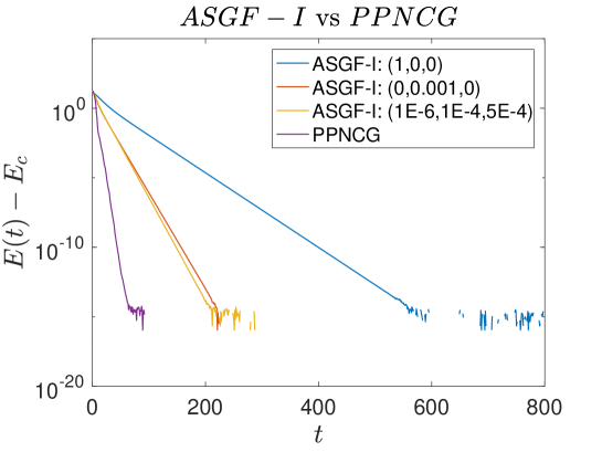
Figure 3: Time evolution of relative energy $E(\Phi_{S}(\textperiodcentered,t))-E_{c}$ (in logarithmic scale) by different numerical schemes when computing the vortex steady state solution. The triplet, for example $(1,0,0)$ in the inset, represents $\alpha_{0i}=1,\alpha_{1i}=0,\alpha_{2i}=0\ (i=1,2)$. The PPNCG method outperforms all others.

Example 3.3. Finally, We apply the PPNCG method to obtain some numerical solutions of the binary GP model. We choose initial datum $\Phi_{S}^{0}(r)=(\sqrt{\alpha}\Phi^{0}(r),\sqrt{1-\alpha}\Phi^{0}(r))^{T}$, where $\Phi^{0}(r)=\frac{1}{\sqrt{\pi S!}}r^{S}e^{-r^{2}/2}$, $\eta=0$, $H_{0}=10$, $\alpha=0.8$, $\gamma=5\pi$, and $V_{1}(r)=V_{2}(r)=\frac{\gamma}{8\pi}r^{2}$. We use the same stopping criterion as alluded to early. In Fig. 4, we depict numerical results of symmetric states $\Phi_{S}^{s}$ and vortex steady states $\Phi_{S}^{c}$ with some selected values of $S$ and $\beta$. In Fig. 5 and 6, we show changes of mass in each component ($N(\phi_{j})=\|\phi_{j}\|^{2},j=1,2$), energy $E_{c}:=E(\Phi_{S}^{c})$, and chemical potential $\mu_{c}:=\mu(\Phi_{S}^{c})$of the vortex steady states with respect to different microwave detuning parameter $\eta$ and background magnetic field $H_{0}$.

From Fig. 4, we observe that (i). as the strength of interaction $\beta$ increases, the radius of vortex annuli in the ground state decreases; (ii). as winding number $S$ increases, the concentrated (peak) density increases as well. The results show that $\eta$ is nearly proportional to the mass difference between two states. Whenever $\eta=0$, $N(\phi_{1})\equiv N(\phi_{2})$. When $|\eta|>>1$, one of the two components of vortex steady states dominates and becomes the only possible state in the limit. From Fig. 6, we observe that there is only one state when $H_{0}=0$ for some small $\beta$ or large $|\eta|$. However, there are two states when $H_{0}\neq 0$. $S=0$ is exactly the one that makes the energy the smallest in comparison with $S\neq 0$, which implies the ground state is spherically symmetric in the general case.

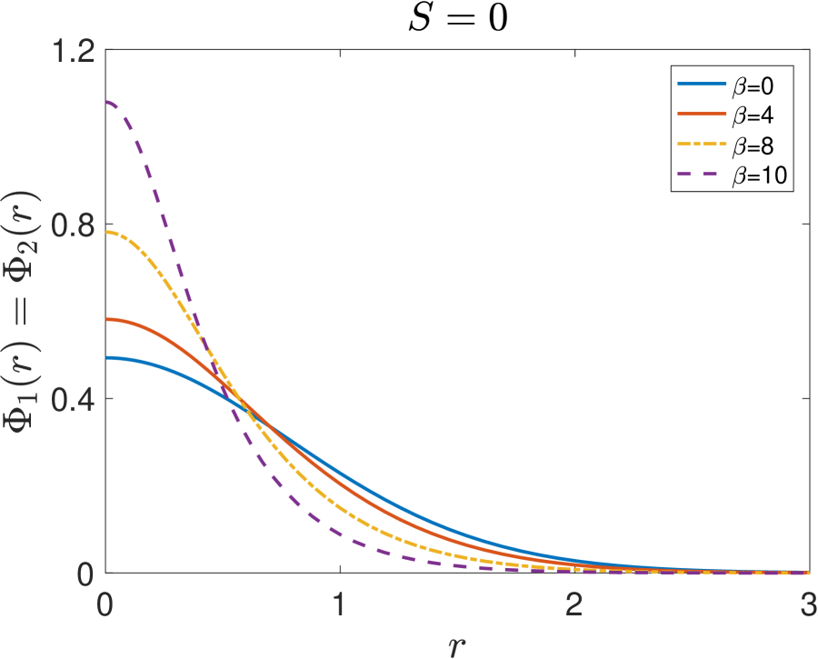
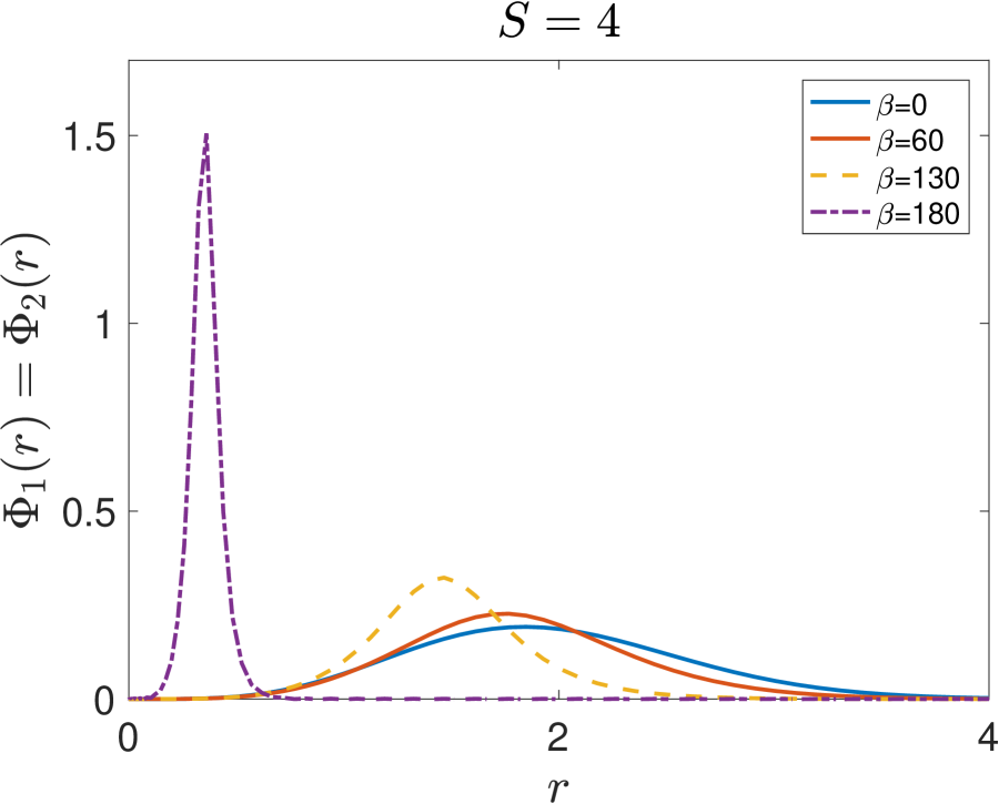
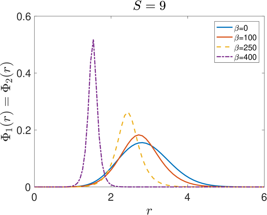
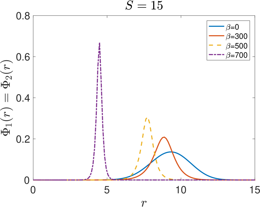
Figure 4: The annular wave function. The radially dependent wave function is depicted with respect to winding number S=0,4,9,15, respectively. As $\beta$ increases, the radius of the ring expands.

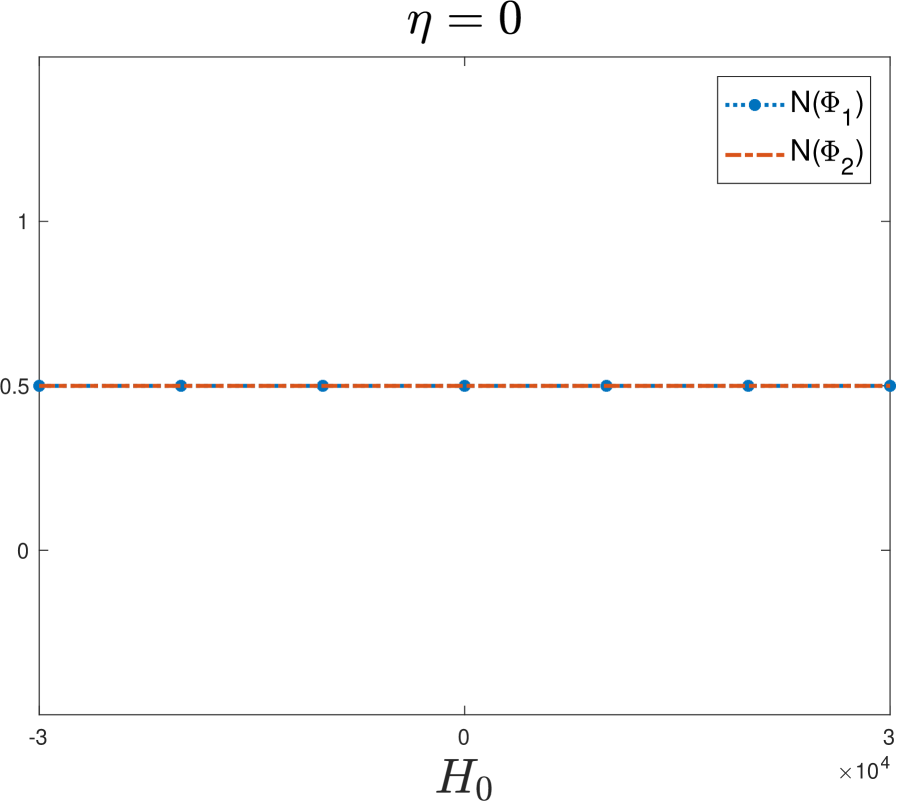
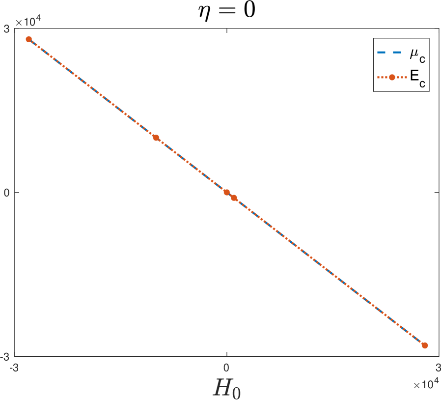
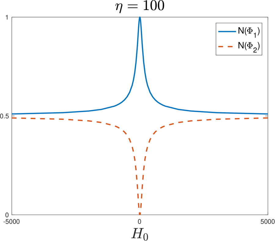
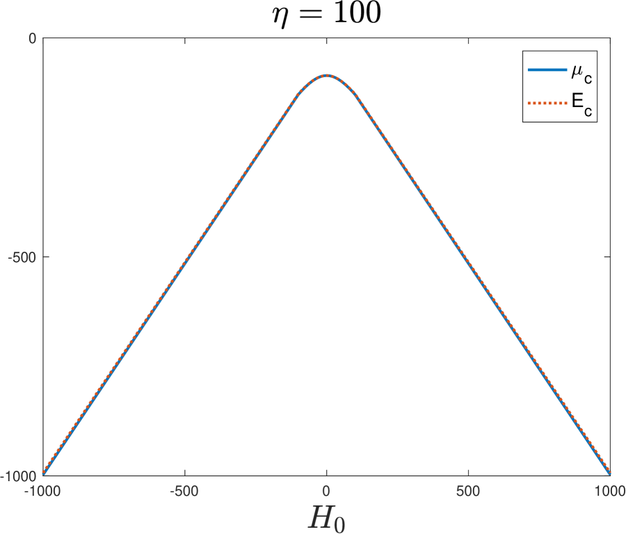
Figure 5: Mass of each component $N(\phi_{j})=\|\phi_{j}\|^{2},j=1,2$, energy $E_{c}$ and chemical potential $\mu_{c}$ in vortex steady states. Variation of mass, energy and chemical potential with respect to $H_{0}$ at $S=13$ and $\beta=300$ when $\eta=0$ (Upper) and when $\eta=100$ (Lower). The role of the microwave detuning number $\eta$ dominate the mass difference between two states.

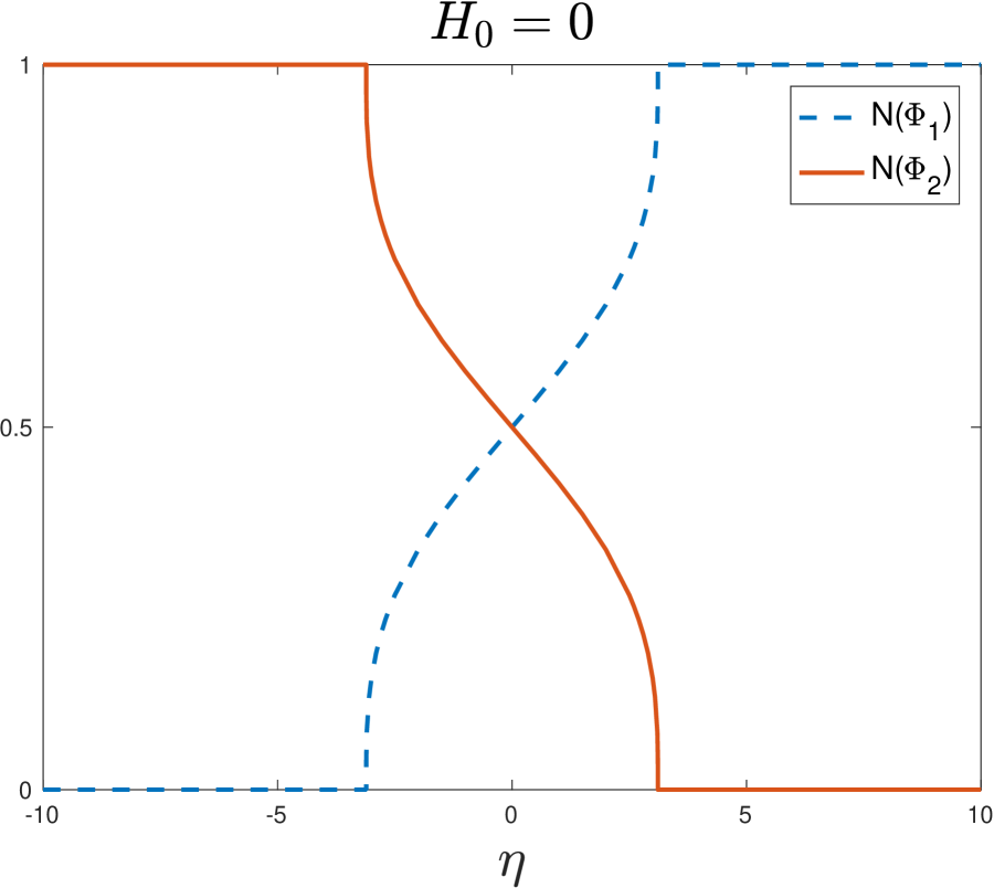
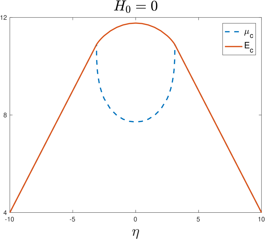
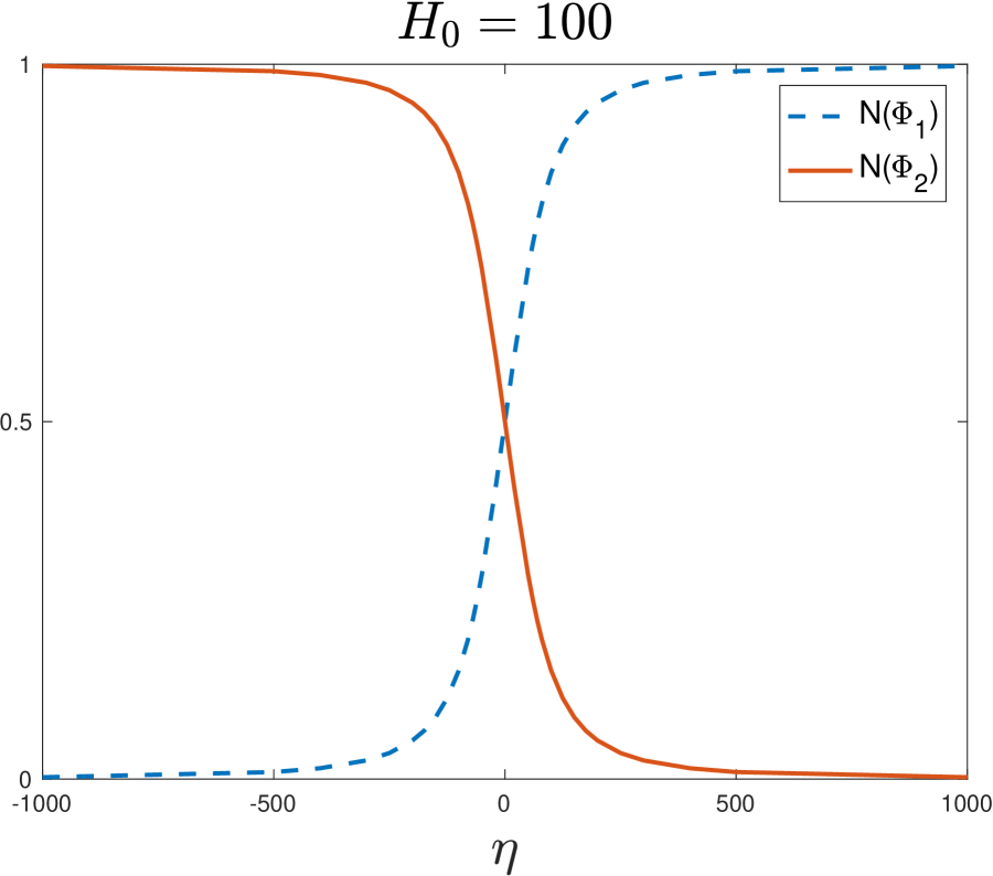
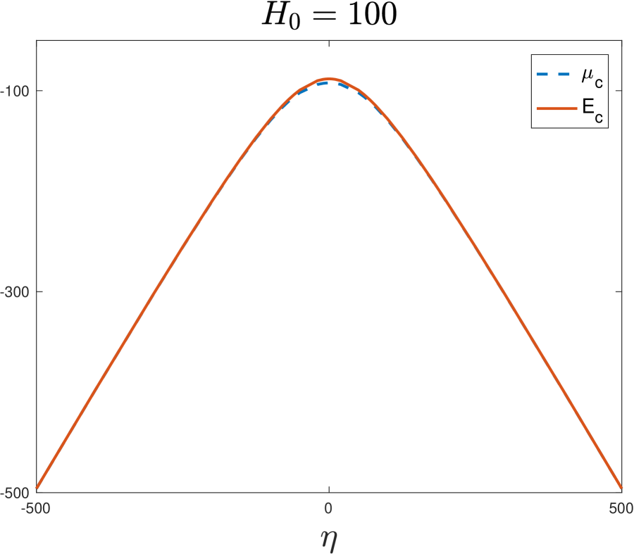
Figure 6: Mass of each component $N(\phi_{j})=\|\phi_{j}\|^{2},j=1,2$, energy $E_{c}$ and chemical potential $\mu_{c}$ in vortex steady states. Variation of mass, energy and chemical potential with respect to $\eta$ at $S=13$ and $\beta=300$ when $H_{0}=0$ (Upper) and when $H_{0}=100$ (Lower). The role of the background magnetic field $H_{0}$ is to smooth the mass and chemical potential curve at the transition values so that the other component is not absolutely absent at large $\eta$ and small $\beta$.

4 Conclusion

We have developed two constrained minimization algorithms for two steady GP equations coupled with magnetic field, equivalent to two nonlocal GP systems, based on the normalized gradient flow model and the perturbed, projected conjugate gradient approach, respectively. These methods are firstly presented using the single component GP model, and later extended to the binary GP model. Detailed comparisons among the new algorithms and the existing GFLM method when computing symmetric and central vortex state solutions of the GP models are conducted in 2D space. The comparative study shows that the ASGF method is significantly better than the GFLM method, while the PPNCG scheme outperforms the ASGF scheme in all the cases investigated. These new methods can be readily extended to other GP equation systems with different external potentials or without the magnetic field coupling, adding additional, efficient computational tools for GP systems.

References

[1]
P.-A. Absil, R. Mahony, and R. Sepulchre.
Optimization Algorithms on Matrix Manifolds.
Princeton University Press, 2009.
[2]
C.S. Adams, M. Sigel, and J. Mlynek.
Atom optics.
Phys. Rep., 240(3):143–210, 1994.
[3]
S.K. Adhikari.
Numerical solution of the two-dimensional Gross–Pitaevskii
equation for trapped interacting atoms.
Phys. Lett. A, 265(1):91–96, 2000.
[4]
S. Agmon.
Lectures on exponential decay of solutions of second-order
elliptic equations: Bounds on Eigenfunctions of N-Body Schrodinger
Operations.Princeton University Press, 2014.
[5]
M.F. Andersen, C. Ryu, P. Cladé, V. Natarajan, A. Vaziri, K. Helmerson, and
W.D. Phillips.
Quantized Rotation of Atoms from Photons with Orbital Angular
Momentum.
Phys. Rev. Lett., 97:170406, 2006.
[6]
X. Antoine and R. Duboscq.
Robust and efficient preconditioned Krylov spectral solvers for
computing the ground states of fast rotating and strongly interacting
Bose–Einstein condensates.
J. Comput. Phys., 258:509–523, 2014.
[7]
X. Antoine and R. Duboscq.
Modeling and Computation of Bose-Einstein Condensates:
Stationary States, Nucleation, Dynamics, Stochasticity, pages 49–145.
Springer International Publishing, Cham, 2015.
[8]
X. Antoine, A. Levitt, and Q. Tang.
Efficient spectral computation of the stationary states of rotating
Bose–Einstein condensates by preconditioned nonlinear conjugate gradient
methods.
J. Comput. Phys., 343:92–109, 2017.
[9]
H. Attouch, X. Goudou, and P. Redont.
The heavy ball with friction method. I. The continuous dynamical
system: global exploration of the local minima of a real-valued function by
asymptotic analysis of a dissipative dynamical system.
Commun. Contemp. Math., 2(1):1–34, 2000.
[10]
W. Bao and Y. Cai.
Mathematical theory and numerical methods for Bose-Einstein
condensation.
Kinet. Relat. Models, 6(1):1–135, 2013.
[11]
W. Bao and Y. Cai.
Mathematical models and numerical methods for Spinor Bose-Einstein
condensates.
Commun. Comput. Phys., 24(4):899–965, 2018.
[12]
W. Bao, I-L. Chern, and F.Y. Lim.
Efficient and spectrally accurate numerical methods for computing
ground and first excited states in Bose–Einstein condensates.
J. Comput. Phys., 219(2):836–854, 2006.
[13]
W. Bao and Q. Du.
Computing the ground state solution of Bose-Einstein condensates by
a normalized gradient flow.
SIAM J. Sci. Comput., 25:1674–1697, 2004.
[14]
W. Bao and J. Shen.
A generalized-Laguerre–Hermite pseudospectral method for computing
symmetric and central vortex states in Bose–Einstein condensates.
J. Comput. Phys., 227(23):9778–9793, 2008.
[15]
W. Bao and W Tang.
Ground-state solution of Bose–Einstein condensate by directly
minimizing the energy functional.
J. Comput. Phys., 187(1):230–254, 2003.
[16]
W. Bao and H. Wang.
A mass and magnetization conservative and energy-diminishing
numerical method for computing ground state of spin-1 Bose-Einstein
condensates.
SIAM J. Numer. Anal., 45(5):2177–2200, 2007.
[17]
W. Bao, H. Wang, and P.A. Markowich.
Ground, symmetric and central vortex states in rotating
Bose-Einstein condensates.
Commun. Math. Sci., 3(1):57–88, 2005.
[18]
D. Baye and J.M. Sparenberg.
Resolution of the Gross–Pitaevskii equation with the
imaginary-time method on a Lagrange mesh.
Phys. Rev. E, 82(5), 2010.
[19]
M. Betancourt, M.I. Jordan, and A.C. Wilson.
On symplectic optimization.
arXiv preprint arXiv:1802.03653, 2018.
[20]
E. Bostan, M. Soltanolkotabi, D. Ren, and L. Waller.
Accelerated Wirtinger Flow for Multiplexed Fourier Ptychographic
Microscopy.
2018 25th IEEE International Conference on Image Processing
(ICIP), pages 3823–3827, 2018.
[21]
Y. Cai and W. Liu.
Efficient and accurate gradient flow methods for computing ground
states of spinor Bose-Einstein condensates.
J. Comput. Phys., 433:110183, 22, 2021.
[22]
M. Caliari, A. Ostermann, S. Rainer, and M. Thalhammer.
A minimisation approach for computing the ground state of
Gross–Pitaevskii systems.
J. Comput. Phys., 228(2):349–360, 2009.
[23]
E. Cancés, R. Chakir, and Y. Maday.
Numerical analysis of nonlinear eigenvalue problems.
J. Sci. Comput., 45(1-3):90–117, 2010.
[24]
E. Cancés and N. Mourad.
A numerical study of the extended Kohn-Sham ground states of
atoms.
Commun. Appl. Math. Comput. Sci., 13(2):139–188, 2018.
[25]
C. Canuto, M.Y. Hussaini, A. Quarteroni, and T.A. Zang.
Spectral Methods in Fluid Dynamicss.
Springer-Verlag, Berlin, New York, 1987.
[27]
M.M. Cerimele, M.L. Chiofalo, F. Pistella, S. Succi, and M.P. Tos.
Numerical solution of the Gross–Pitaevskii equation using an
explicit finite-difference scheme: an application to trapped Bose–Einstein
condensates.
Phys. Rev. E, 62(1):1382–1389, 2000.
[28]
J.-H. Chen, I.-L. Chern, and W Wang.
Exploring ground states and excited states of spin-1 Bose–Einstein
condensates by continuation methods.
J. Comput. Phys., 230(6):2222–2236, 2011.
[29]
P. M. Chesler, A. M. García-García, and H. Liu.
Defect Formation beyond Kibble-Zurek Mechanism and Holography.
Phys. Rev. X, 5:021015, May 2015.
[30]
M.L. Chiofalo, S. Succi, and M.P. Tosi.
Ground state of trapped interacting Bose-Einstein condensates by an
explicit imaginary-time algorithm.
Phys. Rev. E, 62:7438–7444, Nov 2000.
[31]
F. Dalfovo, S. Giorgini, L.P. Pitaevskii, and S. Stringari.
Theory of Bose-Einstein condensation in trapped gases.
Rev. Mod. Phys., 71:463–512, Apr 1999.
[32]
I. Danaila and F. Hecht.
A finite element method with mesh adaptivity for computing vortex
states in fast-rotating Bose–Einstein condensates.
J. Comput. Phys., 229(19):6946–6960, 2010.
[33]
I. Danaila and P. Kazemi.
A new Sobolev gradient method for direct minimization of the
Gross-Pitaevskii energy with rotation.
SIAM J. Sci. Comput., 32(5):2447–2467, 2010.
[34]
I. Danaila and B. Protas.
Computation of ground states of the Gross-Pitaevskii functional
via Riemannian optimization.
SIAM J. Sci. Comput., 39(6):B1102–B1129, 2017.
[35]
C.M. Dion and E. Cancès.
Ground state of the time-independent Gross–Pitaevskii equation.
Comput. Phys. Commun., 177(10):787–798, 2007.
[36]
S.S. Du, C. Jin, J.D. Lee, M.I. Jordan, A. Singh, and B. Poczos.
Gradient descent can take exponential time to escape saddle points.
In Advances in Neural Information Processing Systems, page
1067–1077, 2017.
[37]
A. Edelman, T.A. Arias, and S.T. Smith.
The geometry of algorithms with orthogonality constraints.
SIAM J. Matrix Anal. Appl., 20:303–353, 1998.
[38]
E. Faou and T. Jézéquel.
Convergence of a normalized gradient algorithm for computing ground
states.
IMA J. Numer. Anal., 38:360–376, 2018.
[39]
B. Fornberg.
A pseudospectral approach for polar and spherical geometries.
SIAM J. Sci. Comput., 16:1071–1081, 1995.
[40]
S. Giorgini, L.P. Pitaevskii, and S. Stringari.
Theory of ultracold atomic Fermi gases.
Rev. Mod. Phys., 80:1215–1274, Oct 2008.
[41]
G. Grynberg and C. Robilliard.
Cold atoms in dissipative optical lattices.
Phys. Rep., 355(5):335–451, 2001.
[42]
Z. Hadzibabic, P. Krüger, M. Cheneau, B. Battelier, and J Dalibard.
Berezinskii–Kosterlitz–Thouless crossover in a trapped atomic
gas.
Nature, 441:1118–1121, 2006.
[43]
E.A.L. Henn, J.A. Seman, G. Roati, K.M.F. Magalhães, and V.S. Bagnato.
Emergence of Turbulence in an Oscillating Bose-Einstein Condensate.
Phys. Rev. Lett., 103:045301, Jul 2009.
[44]
C. Jin, P. Netrapalli, and M.I. Jordan.
Accelerated gradient descent escapes saddle points faster than
gradient descent.
in Proc. COLT’18, 2018.
[45]
Y. Kawaguchi and M. Ueda.
Spinor Bose–Einstein condensates.
Phys. Rep., 520(5):253–381, 2012.
[46]
W. Kwon, G. Moon, S. Seo, and Y. Shin.
Critical velocity for vortex shedding in a Bose-Einstein
condensate.
Phys. Rev. A, 91:053615, May 2015.
[47]
W. Liu and Y. Cai.
Normalized gradient flow with Lagrange multiplier for computing
ground states of Bose-Einstein condensates.
SIAM J. Sci. Comput., 43(1):B219–B242, 2021.
[48]
K.W. Madison, F. Chevy, W. Wohlleben, and J. Dalibard.
Vortex formation in a stirred Bose–Einstein condesate.
Phys. Rev. Lett., 84:806–809, 2000.
[49]
N.J. Mauser and Y. Zhang.
Exact Artificial Boundary Condition for the Poisson Equation in the
Simulation of the 2D Schrödinger-Poisson System.
Commun. Comput. Phys., 3:764–780, 2014.
[50]
T.W. Neely, A.S. Bradley, E.C. Samson, S.J. Rooney, E.M. Wright, K.J.H. Law,
R. Carretero-González, P.G. Kevrekidis, M.J. Davis, and B.P. Anderson.
Characteristics of Two-Dimensional Quantum Turbulence in a
Compressible Superfluid.
Phys. Rev. Lett., 111:235301, Dec 2013.
[51]
Y. Nesterov.
A method of solving a convex programming problem with convergence
rate .
in Doklady AN SSSR (translated as Soviet Mathematics Doklady),
269:543–547, 1983.
[52]
Y. Nesterov.
Lectures on Convex Optimization.
Springer, 2018.
[53]
M. O’Neill and S. J. Wright.
Behavior of accelerated gradient methods near critical points of
nonconvex functions.
Math. Program., page 1–25, 2017.
[54]
R. Pugatch, M. Shuker, O. Firstenberg, A. Ron, and N. Davidson.
Topological Stability of Stored Optical Vortices.
Phys. Rev. Lett., 98:203601, May 2007.
[55]
J. Qin, G. Dong, and B.A. Malomed.
Stable giant vortex annuli in microwave-coupled atomic condensates.
Phys. Rev. A, 94(5), 2016.
[56]
D.S. Rokhsar.
Vortex stability and persistent currents in trapped Bose-gas.
Phys. Rev. Lett., 79:2164–2167, 1997.
[57]
J. Shen.
Efficient spectral-Galerkin methods III. Polar and cylindrical
geometries.
SIAM J. Sci. Comput., 1997.
[58]
M. Shuker, O. Firstenberg, R. Pugatch, A. Ron, and N. Davidson.
Storing Images in Warm Atomic Vapor.
Phys. Rev. Lett., 100:223601, Jun 2008.
[59]
T. Simula, M. J. Davis, and K. Helmerson.
Emergence of Order from Turbulence in an Isolated Planar
Superfluid.
Phys. Rev. Lett., 113:165302, Oct 2014.
[60]
T.P. Simula and P.B. Blakie.
Thermal Activation of Vortex-Antivortex Pairs in
Quasi-Two-Dimensional Bose-Einstein Condensates.
Phys. Rev. Lett., 96:020404, Jan 2006.
[61]
G.W. Stagg, A.J. Allen, N.G. Parker, and C.F. Barenghi.
Generation and decay of two-dimensional quantum turbulence in a
trapped Bose-Einstein condensate.
Phys. Rev. A, 91:013612, Jan 2015.
[62]
S.-W. Su, S.-C. Gou, A. Bradley, O. Fialko, and J. Brand.
Kibble-Zurek Scaling and its Breakdown for Spontaneous Generation of
Josephson Vortices in Bose-Einstein Condensates.
Phys. Rev. Lett., 110:215302, May 2013.
[63]
Y. Sun, N. Flammarion, and M. Fazel.
Escaping from saddle points on Riemannian manifolds.
arXiv:1906.07355, 2019.
[64]
T. Tian, Y. Cai, X. Wu, and Z. Wen.
Ground states of spin- Bose-Einstein condensates.
SIAM J. Sci. Comput., 42(4):B983–B1013, 2020.
[65]
D. Wang, Y. Cai, and Q. Wang.
Central vortex steady states and dynamics of Bose–Einstein
condensates interacting with a microwave field.
Physica D, 419:132852, 2021.
[66]
H. Wang.
A projection gradient method for computing ground state of spin-2
Bose–Einstein condensates.
J. Comput. Phys, 274:473–488, 2014.
[67]
Y.-S. Wang, B.-W. Jeng, and C.-S. Chien.
A Two-Parameter Continuation Method for Rotating Two-Component
Bose-Einstein Condensates in Optical Lattices.
Commun. Comput. Phys., 13(2):442–460, 2013.
[68]
A. Wibisono, A.C. Wilson, and M.I. Jordan.
A variational perspective on accelerated methods in optimization.
in Proc. Natl. Acad. Sci. U.S.A., 2016.
[69]
X. Wu, Z. Wen, and W. Bao.
A regularized Newton method for computing ground states of
Bose-Einstein condensates.
J. Sci. Comput., 73(1):303–329, 2017.
[70]
R. Xu, M. Soltanolkotabi, J.P. Haldar, W. Unglaub, J. Zusman, A.F. Levi, and
R.M. Leahy.
Accelerated Wirtinger flow: A fast algorithm for ptychography.
arXiv preprint arXiv:1806.05546, 2018.
[71]
R. Zeng and Y. Zhang.
Efficiently computing vortex lattices in rapid rotating
Bose–Einstein condensates.
Comput. Phys. Commun., 180(6):854–860, 2009.
[72]
N. Zhang, F. Xu, and H. Xie.
An efficient multigrid method for ground state solution of
Bose-Einstein condensates.
Int. J. Numer. Anal. Model., 16(5):789–803, 2019.
[73]
Q. Zhuang and J. Shen.
Efficient SAV approach for imaginary time gradient flows with
applications to one- and multi-component Bose-Einstein Condensates.
J. Comput. Phys., 396:72–88, 2019.