VarRCWA: An Adaptive High-Order Rigorous Coupled Wave Analysis Method

Abstract

Semi-analytical methods, such as rigorous coupled wave analysis, have been pivotal for numerical analysis of photonic structures. In comparison to other methods, they offer much faster computation, especially for structures with constant cross-sectional shapes (such as metasurface units). However, when the cross-sectional shape varies even mildly (such as a taper), existing semi-analytical methods suffer from high computational cost. We show that the existing methods can be viewed as a zeroth-order approximation with respect to the structure’s cross-sectional variation. We instead derive a high-order perturbative expansion with respect to the cross-sectional variation. Based on this expansion, we propose a new semi-analytical method that is fast to compute even in presence of large cross-sectional shape variation. Furthermore, we design an algorithm that automatically discretizes the structure in a way that achieves a user specified accuracy level while at the same time reducing the computational cost.

1 Introduction

Numerical simulation is a fundamental tool for understanding photonic structures. Among many popular methods, semi-analytical methods, such as rigorous coupled wave analysis (RCWA) [moharam1981rigorous], have been widely used for analyzing such devices as metasurfaces [divitt2019ultrafast], gratings [mohamad2020fast] and waveguides [zhu2020inverse]. In comparison to other methods, such as finite-difference time-domain (FDTD) methods, semi-analytical methods often have much lower computational cost.

This advantage stems from how semi-analytical methods discretize Maxwell’s equations. In contrast to other approaches (e.g., FDTD methods) that discretize the spatial domain fully (i.e., in all three dimensions) [yee1966numerical], semi-analytical methods discretize the spatial domain partially (e.g., in only $x$- and $y$-dimension but not $z$-dimension). This is possible because many photonic structures have a primary light propagation direction (referred in this paper as $z$-direction; see Fig. 2). In some cases, along the light propagation direction, the structure’s cross-sectional shape stays unchanged (e.g., a metasurface unit). Therefore, we do not have to discretize the structure along $z$-direction; instead, light propagation in the structure can be viewed as superposition of individual propagating modes experiencing phase shifts. This is the fundamental view that enables semi-analytical methods to reduce computational cost (see 2.1).

However, this view becomes unsound for many photonic structures wherein along the primary light propagation direction, the structure’s cross section varies [piggott2015inverse, miller2020large]. A common example is photonic waveguides (such as a taper; see Fig. 1-a). To simulate these photonic structures using semi-analytical methods, one has to further discretize the structure along $z$-direction into a series of thin sections [liu2012s4, jing2013analysis] (see Fig. 1-b). In each section, the cross-sectional shape is assumed unchanged, and thereby a semi-analytical method can be used to simulate that section. Yet, this approach requires a large number of sections, which in turn devastate the computational advantage of semi-analytical methods. Apart from the computational cost, it is often unclear how many discrete sections are needed to achieve certain accuracy. In practice, one has to rely on trail and error to choose a proper resolution for sufficient accuracy. Oftentimes, to obtain satisfactory results, multiple runs of the simulation method (each with a different resolution) are needed.

In this work, we overcome these limitations. Our method requires no trial and error, thus much easier to use: provided a photonic structure and a user-specified accuracy level (i.e., a real number), our method automatically decides how to discretize the structure in $z$-direction, aiming to reduce the overall computational cost while achieving the desired accuracy. To obtain simulation results of user-specified accuracy, only one run is needed.

To this end, our core development is twofold: 1) We show that the conventional semi-analytical methods (such as RCWA) are merely zeroth-order approximation with respect to the structure’s cross-sectional variation. Through a novel change of variable, we propose a high-order semi-analytical method, which allows the structure’s cross section to vary over $z$-direction, without discretizing it into thin sections. 2) Leveraging this high-order method, we introduce an algorithm that automatically and adaptively discretizes the structure to achieve a user specified accuracy level. For regions where the cross section varies rapidly in $z$-direction, our algorithm will slice the structure in fine resolution to ensure simulation accuracy; for regions with little cross-sectional variance, it will discretize them coarsely to save computational cost.

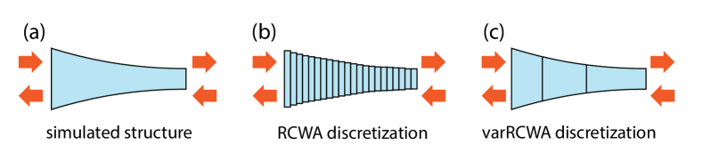
Figure 1: Discretization in conventional and our method. Provided a photonic structure with varying cross-sectional shape (a), conventional semi-analytical methods (such as RCWA) must discretize the structure along the wave propagation direction into many thin sections (b), leading to expensive computation. (c) Our method discretizes the structure adaptively into a much smaller number of sections, thanks to the use of higher-order perturbative expansions. The arrows indicate the incoming and outgoing direction of light waves.

We use our method to analyze various photonic structures, and compare it with conventional semi-analytical methods (such as RCWA). We show that our method, as a higher-order approach, indeed converges faster. As a result, to obtain the same level of accuracy, our method requires much less computational time and no resolution tuning at all.

2 Method

We now present our core development. To understand the rationale behind our development, we start by briefly reviewing the limitations of widely used semi-analytical methods.

2.1 Established Semi-analytical Methods and Their Limitations

Semi-analytical methods discretize the spatial domain of Maxwell’s equations in $x$- and $y$-directions but not in $z$-direction. In frequency domain, Maxwell’s equations become into

$$\frac{\partial\boldsymbol{e}}{\partial z}=\frac{j}{k_{0}}\boldsymbol{P}\boldsymbol{h}\;\textrm{ and }\;\frac{\partial\boldsymbol{h}}{\partial z}=\frac{j}{k_{0}}\boldsymbol{Q}\boldsymbol{e},$$ (1)

where the vectors $\boldsymbol{e}$ and $\boldsymbol{h}$ are discrete representations of the electric and magnetic fields on an $xy$-plane at a $z$ position, and the matrices $\boldsymbol{P}$ and $\boldsymbol{Q}$ encode the distributions of material permeability and permittivity on the $xy$-plane at the same $z$ position. Depending on specific representations of $\boldsymbol{e}$ and $\boldsymbol{h}$, different semi-analytical methods emerge. The most widely used (e.g., for the analysis of metasurfaces [divitt2019ultrafast], gratings [mohamad2020fast] and waveguides [zhu2020inverse]) is rigorous coupled wave analysis (RCWA) method, wherein $\boldsymbol{e}$ and $\boldsymbol{h}$ are discretized using 2D Fourier basis on the $xy$-plane. In this paper, our development can be applied to semi-analytical methods in general (such as the method of lines [pregla1989method]), although our implementation and numerical experiments focus in particular on the RCWA method.

When the structure’s cross-sectional shape is fixed along $z$-direction, both $\boldsymbol{P}$ and $\boldsymbol{Q}$ in eq:pq_form are constant matrices, and Eq. eq:pq_form can be solved through an eigenvalue decomposition, that is, $\boldsymbol{P}\boldsymbol{Q}=\boldsymbol{W}\boldsymbol{\Lambda}^{2}\boldsymbol{W}^{-1}$. The resulting $\boldsymbol{W}$ and $\boldsymbol{\Lambda}$ allow us to express the solution of eq:pq_form as

$$\boldsymbol{e}=\frac{1}{2}\boldsymbol{W}\left(e^{\boldsymbol{\Lambda}z}\boldsymbol{a}_{L}+e^{-\boldsymbol{\Lambda}z}\boldsymbol{b}_{L}\right)\quad\text{and}\quad\boldsymbol{h}=\frac{1}{2}\boldsymbol{V}\left(e^{\boldsymbol{\Lambda}z}\boldsymbol{a}_{L}-e^{-\boldsymbol{\Lambda}z}\boldsymbol{b}_{L}\right).$$ (2)

Here $\boldsymbol{V}$ is the basis for describing the cross-sectional magnetic field, related to the eigenvectors $\boldsymbol{W}$ (i.e., the basis for electric field) through $\boldsymbol{V}=\boldsymbol{Q}\boldsymbol{W}\boldsymbol{\Lambda}^{-1}$; $\boldsymbol{a}_{\textrm{L}}$ and $\boldsymbol{b}_{\text{L}}$ are vectors stacking the coefficients of the forward and backward light waves at the left end of the structure (see Fig. 2). In addition, from Eq. eq:eh_sol, we can define the structure’s scattering matrix, which relates the output state of an optical wave after propagating through the structure with its input state, namely

$$\bmatrix\boldsymbol{a}_{\text{R}}\\ \boldsymbol{b}_{\text{L}}=\boldsymbol{S}\bmatrix\boldsymbol{a}_{\text{L}}\\ \boldsymbol{b}_{\text{R}},\quad\text{where}\;\;\boldsymbol{S}=\bmatrix\boldsymbol{T}_{\text{LR}}&\boldsymbol{R}_{\text{R}}\\ \boldsymbol{R}_{\text{L}}\boldsymbol{T}_{\text{RL}},$$ (3)

where, corresponding to $\boldsymbol{a}_{\text{L}}$ and $\boldsymbol{b}_{\text{L}}$, $\boldsymbol{a}_{\text{R}}$ and $\boldsymbol{b}_{\text{R}}$ describe the forward and backward waves at the right end (see Fig. 2). Once the scattering matrix is known, the structure’s optical performance (e.g., mode conversion efficiency and phase shift of a waveguide) can be directly computed.

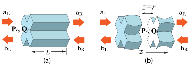
Figure 2: Notation. Provided a photonic structure section, we model light wave propagation in four components: the incoming and outgoing waves at both the left and right ends, as shown by the orange arrows. (a) A section with constant cross-sectional shape has fixed material matrices $\boldsymbol{P}_{r}$ and $\boldsymbol{Q}_{r}$. (b) When a section has a varying cross-sectional shape, we choose a specific position $z=r$ (called reference position), and use the material matrices, $\boldsymbol{P}_{r}$ and $\boldsymbol{Q}_{r}$, at $z=r$ to construct the basis for describing forward and backward waves. Our method treats such a section as a perturbation of a section with constant cross-sectional shape in (a), and leverages a perturbative expansion for numerical simulation. Here for visualization purpose, we cut through the section at $z=r$ to reveal the cross-section at $z=r$, which may differ from the cross-sectional shape at its two ends.

When the structure’s cross-sectional shape varies along $z$-direction, one has to split the structure into a series of small sections so that every section can be approximated as having a fixed cross section (Fig. 1-b). Each section $i$ is then analyzed through the aforementioned process, from which one can compute its scattering matrix $\boldsymbol{S}_{i}$. Finally, by combining all the scattering matrices using Redheffer star product [redheffer1959inequalities], the entire structure’s scattering matrix is obtained.

Limitations.

In semi-analytical methods, the assumption of having a fixed cross section can be viewed as a zeroth-order approximation of the structure (as derived in Sec. 2.2). To achieve sufficient accuracy, such a crude approximation must be remedied with small structure length. As a result, even mild cross-sectional variation requires a large number of discrete sections (Fig. 1-b). For every section, an eigenvalue decomposition is needed, and thus its computational cost is further scaled by the total number of sections. To reduce the computational cost, we need to reduce the total number of discrete sections (Fig. 1-c) while retaining simulation accuracy. This motivates us to seek a high-order semi-analytical method, one that accounts for the cross-sectional variation in a long section and thereby reduces the total number of sections.

2.2 High-order Semi-analytical Methods

Consider a section of photonic structure along $z$-direction. Suppose its cross-sectional shape varies, that is, in Eq. eq:pq_form, $\boldsymbol{P}$ and $\boldsymbol{Q}$ are not constant matrices; they change over $z$. In this case, the solution of eq:pq_form is not as simple as eq:eh_sol. Now, our goal is to express the solution of eq:pq_form as a perturbative expansion with respect to cross-section variation (Fig. 2), and this expansion will serve as the core numerical recipe of our method.

Naïve solution.

To understand the insight of our development, we start with a naïve (but impractical) expansion form of the solution. First, inspired by Eq. eq:eh_sol, we use a set of basis vectors $\boldsymbol{W}$ and $\boldsymbol{V}$ to describe cross-sectional electric and magnetic fields respectively—the specific choice of $\boldsymbol{W}$ and $\boldsymbol{V}$ in presence of varying cross section will be described shortly. The cross-sectional electric and magnetic fields, $\boldsymbol{e}$ and $\boldsymbol{h}$, are formed by light waves propagating forward and backward in the structure, with the relations:

$$\boldsymbol{a}(z)=\boldsymbol{W}^{-1}\boldsymbol{e}(z)+\boldsymbol{V}^{-1}\boldsymbol{h}(z)\;\textrm{ and }\;\boldsymbol{b}(z)=\boldsymbol{W}^{-1}\boldsymbol{e}(z)-\boldsymbol{V}^{-1}\boldsymbol{h}(z),$$ (4)

where $\boldsymbol{a}$ and $\boldsymbol{b}$ are coefficients in the chosen basis for describing the forward and backward waves, respectively, and they vary over $z$. Next, to establish a differential equation of $\boldsymbol{a}$ (and $\boldsymbol{b}$), we differentiate both sides of eq:forward_backward, and then using Maxwell’s equations eq:pq_form, we obtain

$$\frac{\partial\boldsymbol{a}}{\partial z}=\boldsymbol{W}^{-1}\frac{\partial\boldsymbol{e}}{\partial z}+\boldsymbol{V}^{-1}\frac{\partial\boldsymbol{h}}{\partial z}=\frac{j}{2k_{0}}\left[\boldsymbol{W}^{-1}\boldsymbol{P}\boldsymbol{V}\left(\boldsymbol{a}-\boldsymbol{b}\right)+\boldsymbol{V}^{-1}\boldsymbol{Q}\boldsymbol{W}\left(\boldsymbol{a}+\boldsymbol{b}\right)\right].$$ (5)

Equivalently, we have the integral equation

$$\boldsymbol{a}(z)=\boldsymbol{a}(z_{L})+\frac{j}{2k_{0}}\int^{z}_{z_{L}}\left[\left(\boldsymbol{W}^{-1}\boldsymbol{P}\boldsymbol{V}+\boldsymbol{V}^{-1}\boldsymbol{Q}\boldsymbol{W}\right)\boldsymbol{a}(z^{\prime})+\left(\boldsymbol{V}^{-1}\boldsymbol{Q}\boldsymbol{W}-\boldsymbol{W}^{-1}\boldsymbol{P}\boldsymbol{V}\right)\boldsymbol{b}(z^{\prime})\right]{\rm d}z^{\prime},$$ (6)

where $z_{L}$ is the starting $z$ position of the considered structure section. Note also that both $\boldsymbol{P}$ and $\boldsymbol{Q}$ vary over $z$, and a similar integral equation can be obtained for $\boldsymbol{b}(z)$. Equation eq:int_eqn, in theory, allows us to express $\boldsymbol{a}(z)$ as a perturbative expansion. This is achieved by recursively substituting $\boldsymbol{a}(z^{\prime})$ in the integrand with Eq. eq:int_eqn itself up to a certain order (and similarly for $\boldsymbol{b}(z)$). For example, to obtain a first-order expansion, one can replace $\boldsymbol{a}(z^{\prime})$ and $\boldsymbol{b}(z^{\prime})$ in eq:int_eqn with their zeroth-order approximations $\boldsymbol{a}_{L}\approx\boldsymbol{a}(z_{L})$ and $\boldsymbol{b}_{R}\approx\boldsymbol{b}(z_{R})$.

To use this expansion for analyzing a long section (and thereby reduce the total number of sections), the norms of $\boldsymbol{W}^{-1}\boldsymbol{P}\boldsymbol{V}$ and $\boldsymbol{V}^{-1}\boldsymbol{Q}\boldsymbol{W}$ must be sufficiently small—an intuitive explanation of this requirement is provided in Supplement 1. This requirement, however, is hardly satisfied in practice, as both $\boldsymbol{P}$ and $\boldsymbol{Q}$ depend on the cross-sectional material distribution, and their norms may become arbitrarily large. Nevertheless, the development of this expansion motivates a viable strategy: in order to obtain a stable perturbative expansion, we need to avoid using $\boldsymbol{P}$ and $\boldsymbol{Q}$ in an integral equation like eq:int_eqn; instead, we seek an expansion that involves only the variation of $\boldsymbol{P}$ and $\boldsymbol{Q}$ over $z$.

Preconditioned solution.

Our proposed expansion starts with a change of variables. We introduce two variables:

$$\tilde{\boldsymbol{a}}=e^{-\frac{j}{k_{0}}\boldsymbol{\Lambda}z}\boldsymbol{a}\;\textrm{ and }\;\tilde{\boldsymbol{b}}=e^{\frac{j}{k_{0}}\boldsymbol{\Lambda}z}\boldsymbol{b},$$ (7)

where $\boldsymbol{\Lambda}$ is the eigenvalue matrix resulted from eigen-decomposition $\boldsymbol{P}_{r}\boldsymbol{Q}_{r}=\boldsymbol{W}\boldsymbol{\Lambda}^{2}\boldsymbol{W}^{-1}$. Here, $\boldsymbol{P}_{r}$ and $\boldsymbol{Q}_{r}$ are fixed matrices encoding the distribution of material permeability and permittivity at a particular $z=r$ position. Ideally, the cross section at $z=r$ is chosen to represent the “average” cross section over the entire section so that it can be used to construct the basis vectors $\boldsymbol{W}$ and $\boldsymbol{V}$. We therefore refer to this position as the reference position of the section (see Fig. 2-b). While in theory one can choose any $r$ position, in practice we simply use the mid-point of the section. The resulting $\boldsymbol{W}$ (and $\boldsymbol{V}$ through $\boldsymbol{V}=\boldsymbol{QW\Lambda}^{-1}$) is used as the basis for describing forward and backward waves (recall Eq. eq:forward_backward).

This change of variables is the key to introduce the variation of $\boldsymbol{P}$ and $\boldsymbol{Q}$ in an integral equation similar to eq:int_eqn. By differentiating eq:u_d_ph and using Eq. eq:pq_form, we obtain the following differential equations (see the derivation in Supplement 2):

$$\split\frac{\partial\tilde{\boldsymbol{a}}}{\partial z}&=\frac{j}{2k_{0}}e^{\left(-\frac{j}{k_{0}}\boldsymbol{\Lambda}z\right)}\delta\boldsymbol{A}e^{\left(\frac{j}{k_{0}}\boldsymbol{\Lambda}z\right)}\tilde{\boldsymbol{a}}-\frac{j}{2k_{0}}e^{\left(-\frac{j}{k_{0}}\boldsymbol{\Lambda}z\right)}\delta\boldsymbol{B}e^{\left(-\frac{j}{k_{0}}\boldsymbol{\Lambda}z\right)}\tilde{\boldsymbol{b}},\\ \frac{\partial\tilde{\boldsymbol{b}}}{\partial z}=\frac{j}{2k_{0}}e^{\left(\frac{j}{k_{0}}\boldsymbol{\Lambda}z\right)}\delta\boldsymbol{B}e^{\left(\frac{j}{k_{0}}\boldsymbol{\Lambda}z\right)}\tilde{\boldsymbol{a}}-\frac{j}{2k_{0}}e^{\left(\frac{j}{k_{0}}\boldsymbol{\Lambda}z\right)}\delta\boldsymbol{A}e^{\left(-\frac{j}{k_{0}}\boldsymbol{\Lambda}z\right)}\tilde{\boldsymbol{b}},$$ (8)

where $\delta\boldsymbol{A}$ and $\delta\boldsymbol{B}$ are related to the material variation along $z$-direction, namely,

$$\split\delta\boldsymbol{A}(z)=\boldsymbol{W}^{-1}\left(\boldsymbol{P}(z)-\boldsymbol{P}_{r}\right)\boldsymbol{V}+\boldsymbol{V}^{-1}\left(\boldsymbol{Q}(z)-\boldsymbol{Q}_{r}\right)\boldsymbol{W},\\ \delta\boldsymbol{B}(z)=\boldsymbol{W}^{-1}\left(\boldsymbol{P}(z)-\boldsymbol{P}_{r}\right)\boldsymbol{V}-\boldsymbol{V}^{-1}\left(\boldsymbol{Q}(z)-\boldsymbol{Q}_{r}\right)\boldsymbol{W}.$$ (9)

Next, we rewrite Eq. eq:diff_ab in integral forms and replace $\tilde{\boldsymbol{a}}$ and $\tilde{\boldsymbol{b}}$ using Eq. eq:u_d_ph. This leads to a new set of integral equations of $\boldsymbol{a}(z)$ and $\boldsymbol{b}(z)$, ones that differ from eq:int_eqn: a(z) &= e^jk0Λ(z-z_L)a_L+j2k0∫^z_z_Le^jk0Λ(z-z’)δA(z’)a(z’)dz’ - j2k0∫^z_z_Le^jk0Λ(z-z’)δB(z’)b(z’)dz’
b(z) = e^jk0Λ(z_R-z)b_R-