Optimal Transport Tools (OTT):
A JAX Toolbox for all things Wasserstein

Abstract

Optimal transport tools (OTT-JAX) is a python toolbox that can solve optimal transport problems between point clouds and histograms. The toolbox builds on various JAX features, such as automatic and custom reverse mode differentiation, vectorization, just-in-time compilation and accelerators support. The toolbox covers elementary computations, such as the resolution of the regularized OT problem, and more advanced extensions, such as barycenters, Gromov-Wasserstein, low-rank solvers, estimation of convex maps, differentiable generalizations of quantiles and ranks, and approximate OT between Gaussian mixtures. The toolbox code is available at https://github.com/ott-jax/ott

Keywords: optimal transport, Wasserstein distances, Sinkhorn algorithm

1 Background and Motivation: Optimal Transport in a Nutshell

Many areas in science and engineering have to deal with tasks that involve pairing points across two datasets. A minimal working example for such tasks arises when a family of points $(x_{1},\dots,x_{n})$, taken in a space $\mathcal{X}$ has to be matched (registered, assigned, aligned) to another family $(y_{1},\dots,y_{n})$ of the same size, taken in a possibly different space $\mathcal{Y}$. A matching between these two families is a bijective map that assigns to each point $x_{i}$ another point $y_{j}$, and is usually encoded as a permutation $\sigma$. With that convention $x_{i}$ would be assigned to $y_{\sigma_{i}}$, the $\sigma_{i}$-th element in the second family. To define what constitutes a “good” assignment, a practitioner defines an objective $\mathcal{E}$ on permutations. The simplest one is that which is parameterized by a ground cost function $c$ between points, $c:\mathcal{X}\times\mathcal{Y}\rightarrow\mathbb{R}$, to define the objective $\mathcal{E}_{1}(\sigma)=\frac{1}{n}\sum_{i=1}^{n}c(x_{i},y_{\sigma_{i}})$.

Opening a window to more complex transport problems, situations may arise when the user may not have sufficient prior information to define the ground cost function $c$. This arises notably when $\mathcal{X}\neq\mathcal{Y}$ (when $\mathcal{X}=\mathcal{Y}$, $c$ is usually easier to pick, e.g., a distance). In such settings, and because it is comparatively easier to define two cost functions $c_{\mathcal{X}}$ and $c_{\mathcal{Y}}$ defined respectively on $\mathcal{X}\times\mathcal{X}$ and $\mathcal{Y}\times\mathcal{Y}$ (for instance distances), one can consider instead the following objective, that uses a discrepancy function $\Delta$ between reals, $\Delta:\mathbb{R}\times\mathbb{R}\mapsto\mathbb{R}$,

$$\mathcal{E}_{2}(\sigma)=\frac{1}{n^{2}}\sum_{i,i^{\prime}=1}^{n}\Delta\left(\,c_{\mathcal{X}}(x_{i},x_{i^{\prime}}),c_{\mathcal{Y}}(y_{\sigma_{i}},y_{\sigma_{i^{\prime}}}\,)\right)\,.$$

Although energy $\mathcal{E}_{2}$ is slightly harder to parse than $\mathcal{E}_{1}$, its role is to favor permutations $\sigma$ that are as close as possible to an isometry: ideally, if $x_{i}$ is assigned to $y_{\sigma_{i}}$ and $x_{i^{\prime}}$ to $y_{\sigma_{i^{\prime}}}$, one hopes that $c_{\mathcal{X}}(x_{i},x_{i^{\prime}})$ has a value that is close to $c_{\mathcal{Y}}(y_{\sigma_{i}},y_{\sigma_{i^{\prime}}})$. Several issues arise when trying to optimize $\mathcal{E}_{1}$ or $\mathcal{E}_{2}$. The first one lies in the challenge brought forward by optimizing over permutations. This is typically solved by using a relaxation, namely by representing permutations as $n\times n$ matrices with binary entries, with the constraint that each of their rows and columns has exactly one and one only non-zero entry equal to 1. From there, the binary constraint can be relaxed using Birkhoff’s polytope (1946), to focus on bistochastic matrices. The second issue arises when the size of the two families are not the same, and/or weights are associated to the observations, in order to compare two discrete measures $\mu=\sum_{i=1}^{n}a_{i}\delta_{x_{i}}$ and $\nu=\sum_{j=1}^{m}b_{j}\delta_{y_{j}}$. The set of matrices used to represent relaxed permutations is called the transportation polytope, and reads:

$$U(a,b)=\{P\in\mathbb{R}^{n\times m}_{+}\,,P\mathbf{1}_{m}=a,P^{T}\mathbf{1}_{n}=b\},\text{ assuming }a^{T}\mathbf{1}_{n}=b^{T}\mathbf{1}_{m}=1.$$

The focus of the toolbox will be to solve two problems in $U(a,b)$, optimizing the linear and quadratic objectives $\mathcal{E}_{1},\mathcal{E}_{2}$, reformulated to matching a transportation matrix variable $P$:

$$\mathcal{L}_{c}(\mu,\nu) =\min_{P\in U(a,b)}\sum_{i,j=1,1}^{n,m}c(x_{i},y_{j})\,P_{ij}\,.$$ (1)

$$\mathcal{Q}_{c_{\mathcal{X}},c_{\mathcal{Y}}}(\mu,\nu) =\min_{P\in U(a,b)}\sum_{i,i^{\prime},j,j^{\prime}=1,1,1,1}^{n,n,m,m}\Delta\left(\,c_{\mathcal{X}}(x_{i},x_{i^{\prime}}),c_{\mathcal{Y}}(y_{j},y_{j^{\prime}})\,\right)\,P_{ij}P_{i^{\prime}j^{\prime}}\,.$$ (2)

Problems (1) and (2) can be easily extended to a continuous setting. This requires defining joint couplings with marginals $\mu,\nu$, and reformulate the same objectives.

$$\Pi(\mu,\nu) =\{\pi\in\mathcal{P}(\mathcal{X}\times\mathcal{Y}),\forall A,B\subset\mathcal{X}\times\mathcal{Y},\pi(A\times\mathcal{Y})=\mu(A),\pi(\mathcal{X}\times B)=\nu(B)\}$$ (3)

$$\mathcal{L}_{c}(\mu,\nu) =\min_{\pi\in\Pi(\mu,\nu)}\iint_{\mathcal{X}\times\mathcal{Y}}c(x,y)\,\textrm{d}\pi(x,y)$$ (4)

$$\mathcal{Q}_{c_{\mathcal{X}},c_{\mathcal{Y}}}(\mu,\nu) =\min_{\pi\in\Pi(\mu,\nu)}\iint_{\mathcal{X}^{2}}\iint_{\mathcal{Y}^{2}}\Delta\left(\,c_{\mathcal{X}}(x,x^{\prime}),c_{\mathcal{Y}}(y,y^{\prime})\,\right)\textrm{d}\pi(x,y)\textrm{d}\pi(\textrm{x}^{\prime},y^{\prime})\,.$$ (5)

We overload notations here because instantiating (4) and (5) with discrete measures yields back (1) and (2). The relaxation (1), and its continuous extension, are attributed to Kantorovich (1942), while (2) comes from Mémoli (2011). Solving these relaxed problems remains, however, an arduous task. We narrow down on three issues:

1. Scalability. While (1) can be solved using a network-flow solver, known worst-case bounds are super-cubic (Ahuja et al., 1988), e.g. $O(nm(n+m)\log(n+m))$. Problem (2) is NP-hard (notably for $\Delta(u,v)=(u-v)^{2}$), and usually solved heuristically through iterative linearization, to fall back on (1), having to pay repeatedly for that cubic price.

2. Curse of Dimensionality. Most practitioners will likely aim at matching, ideally, densities $\mu,\nu$ as in  (4) and (5), yet, because these densities are likely to be only reachable (notably in high-dimensions) through samples, computations must be carried out using empirical measures $\hat{\mu}_{n}$, $\hat{\nu}_{n}$. Computing $\mathcal{L}_{c}(\hat{\mu}_{n},\hat{\nu}_{n})$ exactly, as in (1) to approach $\mathcal{L}_{c}(\mu,\nu)$, as in (4), is doomed by the curse of dimensionality Fournier and Guillin (2015). In essence, it is akin to wasting compute resources to overfit these samples. Although not as well understood, the curse of dimensionality is likely to be at least (if not more) problematic for $\mathcal{Q}_{c_{\mathcal{X}},c_{\mathcal{Y}}}$.

3. Argmin Diferentiability. While many practitioners might only focus on the value of $\mathcal{L}_{c}$ or $\mathcal{Q}_{c_{\mathcal{X}},c_{\mathcal{Y}}}$, an increasing number of applications may focus instead on optimal $P^{\star}$ matrix solutions. While differentiating $\mathcal{L}_{c}$ or $\mathcal{Q}_{c_{\mathcal{X}},c_{\mathcal{Y}}}$ w.r.t. any of its inputs can be computed using the envelope (a.k.a. Danskin) theorem, variations in $P^{\star}$ are far less smooth. For instance, the Jacobian $J_{x_{i}}P^{\star}$ of the optimal transport matrix w.r.t. an arbitrary input point $x_{i}$ is almost everywhere $0$ (the optimal match is usually not affected by an infinitesimal change).

The goal of OTT is to solve variants of the original OT problems having these issues in mind. Entropic regularization (Cuturi, 2013) is known to help with all three items, notably statistical aspects (Genevay et al., 2019; Mena and Niles-Weed, 2019) and differentiability, using either unrolling (Adams and Zemel, 2011; Bonneel et al., 2016) or implicit differentiation  (Luise et al., 2018; Cuturi et al., 2020). The Low-Rank Sinkhorn approach (Scetbon et al., 2021a) addresses computational challenges further, by imposing a low-rank structure for $P^{\star}$, which can also be leveraged for the quadratic case (Scetbon et al., 2021b).

2 Implementation

We review in this section the essential components of the toolbox.

geometry folder.

The Geometry class and inherited classes that build on it can be thought as encapsulating the mathematical properties of cost matrices $[c(x_{i},y_{j})]_{ij}$, $[c_{\mathcal{X}}(x_{i},x_{i^{\prime}})]_{ii^{\prime}}$ or $[c_{\mathcal{Y}}(y_{j},y_{j^{\prime}})]_{jj^{\prime}}$ appearing in either or both Problem (1) and Problem (2), with the aim of not having to store them as matrices $C$ in memory. For instance, (i) when the cost is the squared-Euclidean norm of vectors in $\mathbb{R}^{d}$ (the scenario considered when instatiating a PointCloud geometry), it is known that $C$ has rank up to $d+2$, making an exact storage of all $n\times m$ distances useless; (ii) when measures are supported in a grid that is the Cartesian product of $d$ univariate discretizations, the cost matrix $C$ would be theoretically of size $n^{d}\times n^{d}$, but applying $C$ or its kernel $e^{-C/\varepsilon}$ can be carried out in $O(dn^{d+1})$ operations.

core folder.

The core section of the toolbox holds all of the crucial ingredients required to solve approximately both (1) and, consequently, (2).

• Problem definitions, problems.py,quad_problems.py: Problems are classes that describe a task to be solved. These problems can be defined in various flavours, either linear, or, possibly, quadratic and even fused. They essentially contain a Geometry object with probability weights.

• Entropic and Low-Rank Sinkhorn Solvers, sinkhorn.py,sinkhorn_lr.py: Solvers to solve iteratively (1), using either a Sinkhorn approach or low-rank constraints.

• Entropic and Low-Rank Gromov Solvers, gromov_wasserstein.py: Solver class to address (2), by making iterated calls to linear problems instantiated above.

• Regularized Barycenters, discrete_barycenter.py: Computation of barycenters between discrete measures, assuming the support of the barycenter is fixed.

• Neural Potentials, icnn.py: input-convex neural networks (Amos et al., 2017).

tools folder.

• Soft-sorting, soft_sort.py: implements ideas from Cuturi et al. (2019, 2020) that highlight OTT’s ability to differentiate through the optimal solutions $P^{\star}$ of (1).

• Gaussian Mixtures folder computes a Wasserstein-like distance between Gaussian mixtures from Delon and Desolneux (2020), which can be used to fit pairs of GMMs with a map between them.

3 Applications

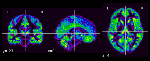
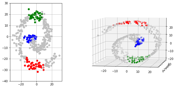
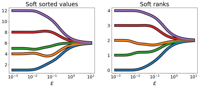
A typical OTT pipeline involves instantiating geom = PointCloud(x, y, cost=...), a geometry from points, where x and y are respectively $n\times d$ and $m\times d$ matrices, possibly endowed with a custom cost function. Specifying next two marginal probability vectors of size $n$ and $m$, a and b, one can define an OT problem, prob=LinearProblem(geom, a, b)) to which a Sinkhorn solver, or a LR Sinkhorn solver can be applied, out= Sinkhorn()(prob) or out= LRSinkhorn(rank=r)(prob). The output encapsulates the transport’s properties, such as, naturally, an out.matrix. Figure 1 shows several advanced applications of OTT-JAX that demonstrates new algorithms combined with differentiability. Details of a wide selection of advances applications, including that of those in Figure 1, are in the toolbox’s documentation as Jupyter Notebooks, which can easily run online without any setup using Colab.

Figure 1: Three advanced applications using OTT-JAX: (left) regularized $W_{p}^{p}$ iso-barycenter of Voxel-Based Morphometry on Oasis dataset, computed efficiently using grid geometry. (middle) Gromov Wasserstein problem matching a spiral in 2 dimensions and a Swiss roll in 3 dimensions where associated points are in the same color.(right) soft-sorted array $[1.0,5.0,4.0,8.0,12.0]$ with different $\epsilon$ controlling differentiability.

References

- Adams and Zemel (2011) Ryan Prescott Adams and Richard S Zemel. Ranking via sinkhorn propagation. arXiv preprint arXiv:1106.1925, 2011.
- Ahuja et al. (1988) Ravindra K Ahuja, Thomas L Magnanti, and James B Orlin. Network flows. 1988.
- Amos et al. (2017) Brandon Amos, Lei Xu, and J Zico Kolter. Input convex neural networks. In International Conference on Machine Learning, pages 146–155. PMLR, 2017.
- Birkhoff (1946) Garrett Birkhoff. Tres observaciones sobre el algebra lineal. Universidad Nacional de Tucumán Revista Series A, 5:147–151, 1946.
- Bonneel et al. (2016) Nicolas Bonneel, Gabriel Peyré, and Marco Cuturi. Wasserstein barycentric coordinates: histogram regression using optimal transport. ACM Transactions on Graphics, 35(4):71:1–71:10, 2016.
- Cuturi (2013) Marco Cuturi. Sinkhorn distances: lightspeed computation of optimal transport. In Advances in Neural Information Processing Systems 26, pages 2292–2300, 2013.
- Cuturi et al. (2019) Marco Cuturi, Olivier Teboul, and Jean-Philippe Vert. Differentiable ranking and sorting using optimal transport. In Advances in Neural Information Processing Systems, volume 32, 2019.
- Cuturi et al. (2020) Marco Cuturi, Olivier Teboul, Jonathan Niles-Weed, and Jean-Philippe Vert. Supervised quantile normalization for low rank matrix factorization. In International Conference on Machine Learning, pages 2269–2279. PMLR, 2020.
- Delon and Desolneux (2020) Julie Delon and Agnes Desolneux. A wasserstein-type distance in the space of gaussian mixture models. SIAM Journal on Imaging Sciences, 13(2):936–970, 2020.
- Fournier and Guillin (2015) Nicolas Fournier and Arnaud Guillin. On the rate of convergence in Wasserstein distance of the empirical measure. Probability Theory and Related Fields, 162(3-4):707–738, 2015.
- Genevay et al. (2019) Aude Genevay, Lénaic Chizat, Francis Bach, Marco Cuturi, and Gabriel Peyré. Sample complexity of sinkhorn divergences. In Proceedings of the 22th International Conference on Artificial Intelligence and Statistics, 2019.
- Kantorovich (1942) Leonid Kantorovich. On the transfer of masses (in russian). Doklady Akademii Nauk, 37(2):227–229, 1942.
- Luise et al. (2018) Giulia Luise, Alessandro Rudi, Massimiliano Pontil, and Carlo Ciliberto. Differential properties of sinkhorn approximation for learning with wasserstein distance. In Advances in Neural Information Processing Systems, volume 31, 2018.
- Mémoli (2011) Facundo Mémoli. Gromov–Wasserstein distances and the metric approach to object matching. Foundations of Computational Mathematics, 11(4):417–487, 2011.
- Mena and Niles-Weed (2019) Gonzalo Mena and Jonathan Niles-Weed. Statistical bounds for entropic optimal transport: Sample complexity and the central limit theorem. Advances in Neural Information Processing Systems, 32, 2019.
- Scetbon et al. (2021a) Meyer Scetbon, Marco Cuturi, and Gabriel Peyré. Low-rank sinkhorn factorization. In Proceedings of the 38th International Conference on Machine Learning, volume 139, pages 9344–9354. PMLR, 2021a.
- Scetbon et al. (2021b) Meyer Scetbon, Gabriel Peyré, and Marco Cuturi. Linear-time gromov wasserstein distances using low rank couplings and costs. arXiv preprint arXiv:2106.01128, 2021b.