Adaptive Accelerated (Extra-)Gradient Methods with Variance Reduction

Abstract

In this paper, we study the finite-sum convex optimization problem focusing on the general convex case. Recently, the study of variance reduced (VR) methods and their accelerated variants has made exciting progress. However, the step size used in the existing VR algorithms typically depends on the smoothness parameter, which is often unknown and requires tuning in practice. To address this problem, we propose two novel adaptive VR algorithms: Adaptive Variance Reduced Accelerated Extra-Gradient (AdaVRAE) and Adaptive Variance Reduced Accelerated Gradient (AdaVRAG). Our algorithms do not require knowledge of the smoothness parameter. AdaVRAE uses $\mathcal{O}\left(n\log\log n+\sqrt{\frac{n\beta}{\epsilon}}\right)$ gradient evaluations and AdaVRAG uses $\mathcal{O}\left(n\log\log n+\sqrt{\frac{n\beta\log\beta}{\epsilon}}\right)$ gradient evaluations to attain an $\mathcal{O}(\epsilon)$-suboptimal solution, where $n$ is the number of functions in the finite sum and $\beta$ is the smoothness parameter. This result matches the best-known convergence rate of non-adaptive VR methods and it improves upon the convergence of the state of the art adaptive VR method, AdaSVRG. We demonstrate the superior performance of our algorithms compared with previous methods in experiments on real-world datasets.

1 Introduction

Table 1: Our results and comparison with prior works.

Algorithm	General convex	Adaptive
SVRG [18]	-	No
$\text{SVRG}^{++}$ [4]	$\mathcal{O}\left(n\log\frac{\beta}{\epsilon}+\frac{\beta}{\epsilon}\right)$	No
Katyusha [1]	$\mathcal{O}\left(n\log\frac{\beta}{\epsilon}+\sqrt{\frac{n\beta}{\epsilon}}\right)$	No
VARAG [22]	$\mathcal{O}\left(n\min\left\{\log\frac{\beta}{\epsilon},\log n\right\}+\sqrt{\frac{n\beta}{\epsilon}}\right)$	No
VRADA [39]	$\mathcal{O}\left(n\min\left\{\log\log\frac{\beta}{\epsilon},\log\log n\right\}+\sqrt{\frac{n\beta}{\epsilon}}\right)$	No
AdaSVRG [12]	$\mathcal{O}\left(\frac{n\beta}{\epsilon}\right)$ (fixed sized inner loop, only if $\epsilon=\Omega(\frac{\beta}{n})$)	Yes
	$\mathcal{O}\left(n\log\frac{\beta}{\epsilon}+\frac{\beta}{\epsilon}\right)$ (multi-stage)
AdaVRAE (unknown $\beta$) (This Paper)	$\mathcal{O}\left(n\min\left\{\log\log\frac{\beta}{\epsilon},\log\log n\right\}+\sqrt{\frac{n\beta}{\epsilon}}\right)$	Yes
AdaVRAE (known $\beta$) (This Paper)	$\mathcal{O}\left(n\min\left\{\log\log\frac{\beta}{\epsilon},\log\log n\right\}+\sqrt{\frac{n\beta}{\epsilon}}\right)$	No
AdaVRAG (unknown $\beta$) (This Paper)	$\mathcal{O}\left(n\min\left\{\log\log\frac{\beta\log\beta}{\epsilon},\log\log n\right\}+\sqrt{\frac{n\beta\log\beta}{\epsilon}}\right)$	Yes
AdaVRAG (known $\beta$) (This Paper)	$\mathcal{O}\left(n\min\left\{\log\log\frac{\beta}{\epsilon},\log\log n\right\}+\sqrt{\frac{n\beta}{\epsilon}}\right)$	No
Lower Bound [42]	$\Omega\left(n+\sqrt{\frac{n\beta}{\epsilon}}\right)$	-

In this paper, we consider the finite-sum optimization problem in the form of

$$\min_{x\in\mathcal{X}}\left\{\frac{1}{n}\sum_{i=1}^{n}f_{i}(x)+h(x)\right\}$$ (1)

where each function $f_{i}$ is convex and $\beta$-smooth, $h$ is convex and potentially nonsmooth but admitting an efficient proximal operator, and $\mathcal{X}\subseteq\mathbb{R}^{d}$ is a closed convex set. Additionally, we further assume that $\mathcal{X}$ is compact when $\beta$ is unknown. Problem (1) has found a wide range of applications in machine learning, typically in empirical risk minimization problems, and has been extensively studied in the past few years.

Among existing approaches to solve this problem, variance reduced (VR) methods [18, 10, 37, 36] have recently shown significant improvement over the classic stochastic gradient methods such as stochastic gradient descent (SGD) and its variants. For example, in strongly convex problems, VR methods such as [1, 22, 29] can achieve the optimal number of gradient evaluations of $\mathcal{O}\left((n+\sqrt{n\kappa})\log\frac{1}{\epsilon}\right)$ to attain an $\mathcal{O}(\epsilon)$-suboptimal solution, where $\kappa$ is the condition number, which improves over full-batch gradient descent ($\mathcal{O}\left(n\kappa\log\frac{1}{\epsilon}\right)$) and Nesterov’s accelerated gradient descent [33, 34] ($\mathcal{O}\left(n\sqrt{\kappa}\log\frac{1}{\epsilon}\right)$). For general convex problems, the current state-of-the-art VR methods, namely VRADA [39] can find an $\mathcal{O}(\epsilon)$-suboptimal solution using $\mathcal{O}\left(n\log\log n+\sqrt{\frac{n\beta}{\epsilon}}\right)$ gradient evaluations, which nearly-matches the lower bound of $\Omega\left(n+\sqrt{\frac{n\beta}{\epsilon}}\right)$[42].

However, most of existing VR gradient methods have the same limitation as classic gradient methods; that is, they require the prior knowledge of the smoothness parameter in order to set the step size. Lacking this information, one may have to carefully perform hyper-parameter tuning to avoid the situation that the algorithm divergences or converges too slowly due to too large or too small step size. This limitation of gradient methods motivates the development of methods that aim to adapt to unknown problem structures. A notable line of work starting with the influential AdaGrad algorithm has designed a family of gradient descent based methods that set the step size based on the gradients or iterates observed in previous iterations [31, 13, 21, 25, 26, 6, 8, 20, 19, 15, 5, 14]. Remarkably, these works have shown that, in the setting where we have access to the exact full gradient in each iteration, it is possible to match the convergence rates of both unaccelerated and accelerated gradient descent methods without any prior knowledge of the smoothness parameter. These methods have also been analyzed in the stochastic setting under a bounded variance assumption, and they achieve a convergence rate that is comparable to that of SGD.

Given the theoretical and practical success of adaptive methods, it is natural to ask whether one can design VR methods that achieve state of the art convergence guarantees without any prior knowledge of the smoothness parameter. The recent work of [12] gives the first adaptive VR method — AdaSVRG — with the gradient complexity of $\mathcal{O}\left(n\log\frac{\beta}{\epsilon}+\frac{\beta}{\epsilon}\right)$. AdaSVRG builds on the AdaGrad [13] and SVRG algorithms [18], both of which are not accelerated.

Our contributions: In this work, we take this line of work further and design the first accelerated VR methods that do not require any prior knowledge of the smoothness parameter. Our algorithms, Adaptive Variance Reduced Accelerated Extra-Gradient (AdaVRAE) and Adaptive Variance Reduced Accelerated Gradient (AdaVRAG), only use $\mathcal{O}\left(n\log\log n+\sqrt{\frac{n\beta}{\epsilon}}\right)$ and $\mathcal{O}\left(n\log\log n+\sqrt{\frac{n\beta\log\beta}{\epsilon}}\right)$ gradient evaluations respectively to attain an $\mathcal{O}(\epsilon)$-suboptimal solution when $\beta$ is unknown, both of which significantly improve the convergence rate of AdaSVRG. Table 1 compares our algorithms and prior VR methods and Section 2 discusses our algorithmic approaches and techniques. The convergence rate of AdaVRAE matches up to constant factors the best-known convergence rate of non-adaptive VR methods [39, 19]. Both of our algorithms follow a different approach from these methods that is based on extra-gradient and mirror descent, instead of dual averaging.

We demonstrate the efficiency of our algorithms in practice on multiple real-world datasets. We show that AdaVRAG and AdaVRAE are competitive with existing standard and adaptive VR methods while having the advantage of not requiring hyperparameter tuning, and in many cases AdaVRAG outperforms these benchmarks.

1.1 Related work

Variance reduced gradient methods: Variance reduction technique [36, 37, 38, 30, 18, 10] has been proposed to improve the convergence rate of stochastic gradient descent algorithms in the finite sum problem and has since become widely-used in many successful algorithms. Notable improvements can be seen in strongly convex optimization problems where earliest algorithms such as SVRG [18] or SAGA [10] obtain $\mathcal{O}\left((n+\kappa)\log\frac{1}{\epsilon}\right)$ convergence rate compared with $\mathcal{O}\left(\frac{\sigma^{2}\kappa}{\beta\epsilon}\right)$ of plain SGD, with the latter requiring an additional assumption on the $\sigma^{2}$-boundedness of the variance term, i.e., $\mathbb{E}_{i}\left[\left\|\nabla f_{i}(x)-\nabla f(x)\right\|^{2}\right]\leq\sigma^{2}$. However, these non-accelerated methods do not achieve the optimal convergence rate. Recent works such as [29, 1, 22] focus on designing accelerated methods and successfully match the optimal lower bound for strongly convex optimization of $\Omega\left((n+\sqrt{n\kappa})\log\frac{1}{\epsilon}\right)$ given by [23].

In non-strongly convex problems, however, existing works do not yet match the lower bound of $\Omega\left(n+\sqrt{\frac{\beta n}{\epsilon}}\right)$ shown in [42]. The best effort so far can be found in the line of accelerated methods started by [1] and followed by [2, 22, 28] that rely on incorporating the checkpoint in each update. AdaVRAG follows the same idea but offers simpler update and more efficient choice of coefficients that results in a better convergence rate, equivalent to VRADA [39]. By comparison, while VRADA is a dual-averaging scheme, AdaVRAG is a mirror descent method and AdaVRAE is an extra-gradient algorithm.

In a different line of research [3, 16, 43], variance reduction has been applied to non-convex optimization to find critical points with much better convergence rate.

Adaptive methods with variance reduction: There has been extensive research on adaptive methods [13, 21, 35, 41, 11] in the setting where we compute a full gradient in each iteration. However, there are only few works combining adaptive methods with VR techniques in the finite sum setup. Most relevant for our work is AdaSVRG [12]. This algorithm is built upon SVRG which as mentioned earlier is a non-accelerated method and has a slower convergence rate. AdaSVRG uses the gradient norm to update the step size, similar to [13] and the step is reset in every epoch, which could lead to step sizes that are too large in later stages. In contrast, both AdaVRAG and AdaVRAE are accelerated VR methods and use a cumulative step size. AdaVRAG uses the iterate movement to update the step size, as in [6, 15]. AdaVRAE improves the convergence rate by a $\sqrt{\log\beta}$ factor by using the gradient difference similarly to [32, 19, 14].

A different line of work considers VR methods that set the step size using stochastic line search [37, 30] or Barzilai-Borwein step size [40, 27]. The former methods do not have theoretical guarantees, and the latter methods require knowledge of the smoothness parameter in order to obtain theoretical bounds.

Recent works design variance-reduced methods for non-convex optimization. STORM [9] and $\text{STORM}^{+}$[24] design an adaptive step size, though the former still requires the smoothness parameter in the step size. Super-Adam [17] also requires their parameters to satisfy some inequality involving the smoothness parameter like STORM.

1.2 Notation and problem setup

Let $\left[n\right]$ denote the set $\left\{1,2,\cdots,n\right\}$. For simplicity, we only consider the Euclidean norm $\left\|\cdot\right\|\mathrel{\coloneqq}\left\|\cdot\right\|_{2}$ (Our work can be extended to $\left\|x\right\|_{A}\coloneqq\sqrt{x^{\top}Ax}$ for any $A\succ 0$ with almost no change). $x^{+}$ represents $\max\left\{x,0\right\}$.

We are interested in solving the following problem

$$\min_{x\in\mathcal{X}}\left\{F(x)=f(x)+h(x)\right\}$$

where $f(x)\coloneqq\frac{1}{n}\sum_{i=1}^{n}f_{i}(x)$ and for $i\in\left[n\right]$, $f_{i}:\mathbb{R}^{d}\to\mathbb{R}$ and $h:\mathcal{X}\to\mathbb{R}$ are convex functions with a closed convex set $\mathcal{X}\subseteq\mathbb{R}^{d}$. Let $x^{*}=\arg\min_{x\in\mathcal{X}}F(x)$. We say a function $G$ is $\beta$-smooth if $\left\|\nabla G(x)-\nabla G(y)\right\|\leq\beta\left\|x-y\right\|$ for all $x,y\in\mathbb{R}^{d}$. Equivalently, we have $G(y)\leq G(x)+\left\langle\nabla G(x),y-x\right\rangle+\frac{\beta}{2}\left\|y-x\right\|^{2}$. In this paper we always assume that each $f_{i}$ is $\beta$-smooth, which implies that $f$ is also $\beta$-smooth. We assume that we can efficiently solve optimization problems of the form $\arg\min_{x\in\mathcal{X}}\left(\gamma h(x)+\frac{1}{2}\left\|x-v\right\|^{2}\right)$ where $\gamma\geq 0$ and $v\in\mathbb{R}^{d}$. When the smoothness parameter $\beta$ is unknown, we additionally assume that $\mathcal{X}$ is compact with diameter $D$, i.e., $\sup_{x,y\in\mathcal{X}}\left\|x-y\right\|\leq D$.

2 Our algorithms and convergence guarantees

Algorithm 1 AdaVRAE

Input: initial point $u^{(0)}$, domain diameter $D$.

Parameters: $\{a^{(s)}\}$,$\left\{T_{s}\right\}$, $A_{T_{0}}^{(0)}>0$, $\eta>0$.

$\overline{x}_{0}^{(1)}=z_{0}^{(1)}=u^{(0)}$, compute $\nabla f(u^{(0)})$

Initialize $\gamma_{0}^{(1)}=\gamma$, where $\gamma$ is any small constant

for $s=1$ to $S$:

   $A_{0}^{(s)}=A_{T_{s-1}}^{(s-1)}-T_{s}\left(a^{(s)}\right)^{2}$

   for $t=1$ to $T_{s}$:

      $x_{t}^{(s)}=\arg\min_{x\in\mathcal{X}}\left\{a^{(s)}\left\langle g_{t-1}^{(s)},x\right\rangle+a^{(s)}h(x)+\frac{\gamma_{t-1}^{(s)}}{2}\left\|x-z_{t-1}^{(s)}\right\|^{2}\right\}$

      Let $A_{t}^{(s)}=A_{t-1}^{(s)}+a^{(s)}+\left(a^{(s)}\right)^{2}$

      $\overline{x}_{t}^{(s)}=\frac{1}{A_{t}^{(s)}}\left(A_{t-1}^{(s)}\overline{x}_{t-1}^{(s)}+a^{(s)}x_{t}^{(s)}+\left(a^{(s)}\right)^{2}u^{(s-1)}\right)$

       if $t\neq T_{s}$:

         Pick $i_{t}^{(s)}\sim\mathrm{Uniform}\left(\left[n\right]\right)$

         $g_{t}^{(s)}=\nabla f_{i_{t}^{(s)}}(\overline{x}_{t}^{(s)})-\nabla f_{i_{t}^{(s)}}(u^{(s-1)})+\nabla f(u^{(s-1)})$

       else:

         $g_{t}^{(s)}=\nabla f(\overline{x}_{t}^{(s)})$

      $\gamma_{t}^{(s)}=\frac{1}{\eta}\sqrt{\eta^{2}\left(\gamma_{t-1}^{(s)}\right)^{2}+\left(a^{(s)}\right)^{2}\left\|g_{t}^{(s)}-g_{t-1}^{(s)}\right\|^{2}}$

      $z_{t}^{(s)}=\arg\min_{z\in\mathcal{X}}\left\{a^{(s)}\left\langle g_{t}^{(s)},z\right\rangle+a^{(s)}h(z)+\frac{\gamma_{t-1}^{(s)}}{2}\left\|z-z_{t-1}^{(s)}\right\|^{2}+\frac{\gamma_{t}^{(s)}-\gamma_{t-1}^{(s)}}{2}\left\|z-x_{t}^{(s)}\right\|^{2}\right\}$

   $u^{(s)}=\overline{x}_{0}^{(s+1)}=\overline{x}_{T_{s}}^{(s)}$, $z_{0}^{(s+1)}=z_{T_{s}}^{(s)}$, $g_{0}^{(s+1)}=g_{T_{s}}^{(s)}$, $\gamma_{0}^{(s+1)}=\gamma_{T_{s}}^{(s)}$

return $u^{(S)}$

Algorithm 2 AdaVRAG

Input: initial point $u^{(0)}$, domain diameter $D$.

Parameters: $\{a^{(s)}\}$, $a^{(s)}\in(0,1)$, $\{q^{(s)}\}$, $\{T_{s}\}$, $\eta>0$.

$x_{0}^{(1)}=u^{(0)}$

Initialize $\gamma_{0}^{(1)}=\gamma$, where $\gamma$ is any small constant

for $s=1$ to $S$:

   $\overline{x}_{0}^{(s)}=a^{(s)}x_{0}^{(s)}+(1-a^{(s)})u^{(s-1)},$ compute $\nabla f(u^{(s-1)})$

   for $t=1$ to $T_{s}$:

      Pick $i_{t}^{(s)}\sim\mathrm{Uniform}\left(\left[n\right]\right)$

      $g_{t}^{(s)}=\nabla f_{i_{t}^{(s)}}(\overline{x}_{t-1}^{(s)})-\nabla f_{i_{t}^{(s)}}(u^{(s-1)})+\nabla f(u^{(s-1)})$

      $x_{t}^{(s)}=\arg\min_{x\in\mathcal{X}}\left\{\left\langle g_{t}^{(s)},x\right\rangle+h(x)+\frac{\gamma_{t-1}^{(s)}q^{(s)}}{2}\left\|x-x_{t-1}^{(s)}\right\|^{2}\right\}$

      $\overline{x}_{t}^{(s)}=a^{(s)}x_{t}^{(s)}+(1-a^{(s)})u^{(s-1)}$

      Option I: $\gamma_{t}^{(s)}=\gamma_{t-1}^{(s)}\sqrt{1+\frac{\left\|x_{t}^{(s)}-x_{t-1}^{(s)}\right\|^{2}}{\eta^{2}}}$

      Option II: $\gamma_{t}^{(s)}=\gamma_{t-1}^{(s)}+\frac{\left\|x_{t}^{(s)}-x_{t-1}^{(s)}\right\|^{2}}{\eta^{2}}$

   $u^{(s)}=\frac{1}{T_{s}}\sum_{t=1}^{T_{s}}\overline{x}_{t}^{(s)}$, $x_{0}^{(s+1)}=x_{T_{s}}^{(s)}$ $,\gamma_{0}^{(s+1)}=\gamma_{T_{s}}^{(s)}$

return $u^{(S)}$

In this section, we describe our algorithms and state their convergence guarantees. Our algorithm AdaVRAE shown in Algorithm 1 is a novel accelerated scheme that uses past extra-gradient update steps in the inner loop and novel averaging to achieve acceleration. AdaVRAE adaptively sets the step sizes based on the stochastic gradient difference. Our choice of step sizes is a novel adaptation to the VR setting of the step sizes used by the works [32, 20, 19, 14] in the batch/full-gradient setting. Our algorithm builds on the work [14], which provides an unaccelerated past extra-gradient algorithm in the batch/full-gradient setting.

Theorem 2.1 states the parameter choices and the convergence guarantee for AdaVRAE, and we give its proof in Section A in the appendix. The convergence rate of AdaVRAE matches up to constant factors the rate of the state of the art non-adaptive VR methods [19, 39]. The initial step size $\gamma_{0}^{(1)}$ can be set to any small constant $\gamma$, which in practice we choose $\gamma=0.01$. Similarly to AdaGrad, setting $\eta=\Theta(D)$ gives us the optimal dependence of the convergence rate in the domain diameter. For simplicity, we state the convergence in Theorem 2.1 and 2.2 when $\eta=\Theta(D)$. We refer the reader to Theorems A.1 and B.1 in the appendix for the precise choice of parameters as well as the full dependence of the convergence rate on arbitrary choices of $\gamma$ and $\eta$. In both Theorem 2.1 and 2.2, we measure convergence using the number of individual gradient evaluations $\nabla f_{i}$, assuming that the exact computation of $\nabla f$ takes $n$ gradient evaluations.

Theorem 2.1.

(Convergence of AdaVRAE) Define $s_{0}=\left\lceil\log_{2}\log_{2}4n\right\rceil$, $c=\frac{3}{2}$. Suppose we set the parameters of Algorithm 1 as follows:

$$a^{(s)} =\begin{cases}(4n)^{-0.5^{s}}&1\leq s\leq s_{0}\\ \frac{s-s_{0}-1+c}{2c}&s_{0}<s\end{cases},$$

$$T_{s} =n,$$

$$A_{T_{0}}^{(0)} =\frac{5}{4}.$$

Suppose that $\mathcal{X}$ is a compact convex set with diameter $D$ and we set $\eta=\Theta(D)$. The number of individual gradient evaluations to achieve a solution $u^{(S)}$ such that $\mathbb{E}\left[F(u^{(S)})-F(x^{*})\right]\leq\epsilon$ for Algorithm 1 is

$$\#grads =\begin{cases}\mathcal{O}\text{$\left(n\log\log\frac{V_{1}}{\epsilon}\right)$}&\mbox{if }\epsilon\geq\frac{V_{1}}{n}\\ \mathcal{O}\left(n\log\log n+\sqrt{\frac{nV_{1}}{\epsilon}}\right)&\mbox{if }\epsilon<\frac{V_{1}}{n}\end{cases}$$

where $V_{1}=\mathcal{O}\left(F(u^{(0)})-F(x^{*})+\left(\text{$\gamma$}+\beta\right)D^{2}\right)$.

Our algorithm AdaVRAG is shown in Algorithm 2. Compared with AdaVRAE, AdaVRAG has a worse dependence on the smoothness parameter $\beta$ but it performs only one projection onto $\mathcal{X}$ in each inner iteration. Additionally, as we discuss in more detail below, it uses adaptive step sizes based on the iterate movement.

AdaVRAG follows a similar framework to existing VR methods such as VARAG [22] and VRADA [39]. Similarly to VRADA, the algorithm achieves acceleration at the epoch level, where an epoch is an iteration of the outer loop. The iterations in an epoch update the main iterates via mirror descent with novel choices of step sizes and coefficients. The stochastic gradient is computed at a point that is a convex combination between the current iterate and the checkpoint; the coefficients of this combination remain fixed throughout the epoch. The step sizes are adaptively set based on the iterate movement.

The structure of the inner iterations of our algorithm differs from both VARAG and VRADA in several notable aspects. VARAG also uses mirror descent to update the main iterates and it computes the stochastic gradient at suitable combinations of the iterates and the checkpoint. AdaVARAG uses a different averaging of the iterates to compute the snapshots. Moreover, it uses a very different and simpler choice for the coefficient used to combine the main iterates and the checkpoint in order to obtain the points at which the stochastic gradients are evaluated. In VARAG, this coefficient is set to a constant (namely, $1/2$) in the initial iterations, whereas in AdaVRAG, it starts from a small number and is increased gradually. This choice is critical for improving the first term in the convergence from $\mathcal{O}(n\log n)$ to $\mathcal{O}(n\log\log n)$. In a similar manner, VRADA attains the same convergence by a new choice of coefficient. However, this is achieved via a very different approach based on dual-averaging.

The step sizes used by AdaVRAG have two components: the step $\gamma_{t}^{(s)}$ that is updated based on the iterate movement and the per-epoch coefficient $q^{(s)}$ to achieve acceleration at the epoch level. Our analysis is flexible and allows the use of several approaches for updating the steps $\gamma_{t}^{(s)}$. One approach, shown as option I in Algorithm 2, is based on the multiplicative update rule of AdaGrad+ [15] which generalizes the AdaGrad update to the constrained setting. We also propose a different variant, shown as option II, that updates the steps in an additive manner. Our analysis shows a similar convergence guarantee for both options, with the main difference being in the dependence on the smoothness: option I incurs a dependence of $\sqrt{\beta\log\beta}$, whereas option II has a worse dependence of $\beta$. Option II achieved improved performance in our experiments.

Theorem 2.2 states the parameter choices and the convergence guarantee for AdaVRAG, and we give its proof in Section B in the appendix. Analogously to AdaVRAE, the initial step size $\gamma$ can be set to any small constant.

Theorem 2.2.

(Convergence of AdaVRAG) Define $s_{0}=\lceil\log_{2}\log_{2}4n\rceil$, $c=\frac{3+\sqrt{33}}{4}$. Suppose we set the parameters of Algorithm 2 as follows:

$$a^{(s)} =\begin{cases}1-\left(4n\right)^{-0.5^{s}}&1\leq s\leq s_{0}\\ \frac{c}{s-s_{0}+2c}&s_{0}<s\end{cases},$$

$$q^{(s)} =\begin{cases}\frac{1}{\left(1-a^{(s)}\right)a^{(s)}}&1\leq s\leq s_{0}\\ \frac{8\left(2-a^{(s)}\right)a^{(s)}}{3(1-a^{(s)})}&s_{0}<s\end{cases},$$

$$T_{s} =n.$$

Suppose that $\mathcal{X}$ is a compact convex set with diameter $D$ and we set $\eta=\Theta(D)$. Additionally, we assume that $2\eta^{2}>D^{2}$ if Option I is used for setting the step size. The number of individual gradient evaluations to achieve a solution $u^{(S)}$ such that $\mathbb{E}\left[F(u^{(S)})-F(x^{*})\right]\leq\epsilon$ for Algorithm 2 is

$$\#grads=\begin{cases}\mathcal{O}\left(n\log\log\frac{V_{2}}{\epsilon}\right)&\epsilon\geq\frac{V_{2}}{n}\\ \mathcal{O}\left(n\log\log n+\sqrt{\frac{nV_{2}}{\epsilon}}\right)&\epsilon<\frac{V_{2}}{n}\end{cases},$$

where

$$V_{2}=\begin{cases}\mathcal{O}\left(F(u^{(0)})-F(x^{*})+\left(\text{$\gamma$}+\beta\log\left(\frac{\beta}{\gamma}\right)\right)D^{2}\right)&\text{for Option I}\\ \mathcal{O}\left(F(u^{(0)})-F(x^{*})+\left(\text{$\gamma$}+\beta^{2}\right)D^{2}\right)&\text{for Option II}\end{cases}.$$

Comparison to AdaSVRG: As noted in the introduction, the state of the art adaptive VR method is the AdaSVRG algorithm [12], which is a non-accelerated method. Both of our algorithms achieve a faster convergence using different approaches and step sizes. AdaSVRG resets the step sizes in each epoch, whereas our algorithms use a cumulative update approach for the step sizes. In our experimental evaluation, the resetting of the step sizes led to slower convergence. AdaSVRG (multi-stage variant) uses varying epoch lengths similarly to $\text{SVRG}^{++}$ [4], whereas our algorithms use epoch lengths that are set to $n$. Using an epoch of length $n$ allows for implementing the random sampling via a random permutation of $[n]$ and is the preferred approach in practice.

Both our algorithms and AdaSVRG require that the domain $\mathcal{X}$ has bounded diameter. This is a restriction that is shared by almost all existing adaptive methods. Recent work [5, 14] in the batch/full-gradient setting have proposed unaccelerated methods that are suitable for unbounded domains, at a loss of additional factors in the convergence. All of the existing accelerated methods require that the domain is bounded, even in the batch/full-gradient setting. We note that our analysis holds for arbitrary compact domains, whereas the analysis of AdaSVRG only applies to domains that contain the global optimum. Similarly to AdaGrad, both our algorithms and AdaSVRG can be used in the unconstrained setting under the promise that the iterates do not move too far from the optimum.

Non-adaptive variants of our algorithms: In the setting where the smoothness parameter is known, we can set the step sizes of our algorithms based on the smoothness, as shown in Algorithms 3 and 4 (Sections C and D in the appendix). Both algorithms match the convergence rates of the state of the art VR methods [19, 39] using different algorithmic approaches based on mirror descent and extra-gradient instead of dual-averaging. We experimentally compare the non-adaptive algorithms to existing methods in Section E of the appendix.

2.1 Analysis outline

We outline some of the key steps in the analysis of AdaVRAE. For the purpose of simplicity, we assume $h=0$ and $\eta=D$. By building on the standard analysis of the stochastic regret for extra-gradient methods, we obtain the following result for the progress of one iteration:

$$\mathbb{E}\left[\left(A_{t}^{(s)}-\left(a^{(s)}\right)^{2}\right)\left(f(\overline{x}_{t}^{(s)})-f(x^{*})\right)-A_{t-1}^{(s)}\left(f(\overline{x}_{t-1}^{(s)})-f(x^{*})\right)\right]$$

$$\leq\mathbb{E}\left[\frac{\gamma_{t-1}^{(s)}}{2}\left\|z_{t-1}^{(s)}-x^{*}\right\|^{2}-\frac{\gamma_{t}^{(s)}}{2}\left\|z_{t}^{(s)}-x^{*}\right\|^{2}\right]$$

$$+\mathbb{E}\left[\frac{\gamma_{t}^{(s)}-\gamma_{t-1}^{(s)}}{2}\left\|x_{t}^{(s)}-x^{*}\right\|^{2}\right]$$

$$+\mathbb{E}\left[\left(a^{(s)}\right)^{2}\left\langle\nabla f(\overline{x}_{t}^{(s)}),u^{(s-1)}-\overline{x}_{t}^{(s)}\right\rangle\right]$$

$$+\mathbb{E}\left[\frac{\left(a^{(s)}\right)^{2}}{2\gamma_{t}^{(s)}}\left\|g_{t}^{(s)}-g_{t-1}^{(s)}\right\|^{2}\right]$$

$$-\underbrace{\mathbb{E}\left[\frac{A_{t-1}^{(s)}}{2\beta}\left\|\nabla f(\overline{x}_{t}^{(s)})-\nabla f(\overline{x}_{t-1}^{(s)})\right\|^{2}\right]}_{\mbox{gain}}.$$ (2)

In comparison to the standard analysis, the coefficient for the checkpoint appears in the coefficient of $f(\overline{x}_{t}^{(s)})-f(x^{*})$, which becomes $\left(A_{t}^{(s)}-\left(a^{(s)}\right)^{2}\right)$ instead of the usual $A_{t}^{(s)}$, making the sum not telescope immediately. To resolve this, we first turn our attention to the analysis of the stochastic gradient difference $\left\|g_{t}^{(s)}-g_{t-1}^{(s)}\right\|^{2}$. The key idea is to split $\frac{\left(a^{(s)}\right)^{2}}{2\gamma_{t}^{(s)}}\left\|g_{t}^{(s)}-g_{t-1}^{(s)}\right\|^{2}$ into $\left(\frac{1}{2\gamma_{t}^{(s)}}-\frac{1}{16\beta}\right)\left(a^{(s)}\right)^{2}\left\|g_{t}^{(s)}-g_{t-1}^{(s)}\right\|^{2}+\frac{\left(a^{(s)}\right)^{2}}{16\beta}\left\|g_{t}^{(s)}-g_{t-1}^{(s)}\right\|^{2}$, and bound each term in turn. For the first term, we build on the techniques from prior work in the batch/full-gradient setting [14]. For the second term, we use Young’s inequality to write $\mathbb{E}\left[\left\|g_{t}^{(s)}-g_{t-1}^{(s)}\right\|^{2}\right]\leq\mathbb{E}\left[4\left\|\nabla f(\overline{x}_{t}^{(s)})-g_{t}^{(s)}\right\|^{2}+4\left\|\nabla f(\overline{x}_{t-1}^{(s)})-g_{t-1}^{(s)}\right\|^{2}\right]+\mathbb{E}\left[2\left\|\nabla f(\overline{x}_{t}^{(s)})-\nabla f(\overline{x}_{t-1}^{(s)})\right\|^{2}\right]$. The gradient difference loss term is cancelled by the gain term in (2), and thus we can focus on the first two variance terms. We apply the usual variance reduction technique put forward by [22] (see Lemma A.2) to bound the two variance terms, as follows:

$$\mathbb{E}\left[\left\|g_{t}^{(s)}-\nabla f(\overline{x}_{t}^{(s)})\right\|^{2}\right]\leq\mathbb{E}\left[2\beta\left(f(u^{(s-1)})-f(\overline{x}_{t}^{(s)})-\left\langle\nabla f(\overline{x}_{t}^{(s)}),u^{(s-1)}-\overline{x}_{t}^{(s)}\right\rangle\right)\right].$$

Thus we obtain an upper bound on $\frac{\left(a^{(s)}\right)^{2}}{16\beta}\left\|g_{t}^{(s)}-g_{t-1}^{(s)}\right\|^{2}$ in terms of $\left(a^{(s)}\right)^{2}\left(f(u^{(s-1)})-f(\overline{x}_{t}^{(s)})\right)$. This is the reason for setting the coefficient for the checkpoint to $\left(a^{(s)}\right)^{2}$, so that the LHS of (2) can become the usual telescoping sum $A_{t}^{(s)}\left(f(\overline{x}_{t}^{(s)})-f(x^{*})\right)-A_{t-1}^{(s)}\left(f(\overline{x}_{t-1}^{(s)})-f(x^{*})\right)$. Using the convexity of $f$, we obtain the following key result for the progress of each epoch:

$$\mathbb{E}\left[A_{T_{s}}^{(s)}\left(f(\overline{x}_{T_{s}}^{(s)})-f(x^{*})\right)-A_{0}^{(s)}\left(f(\overline{x}_{0}^{(s)})-f(x^{*})\right)\right]$$

$$\leq\mathbb{E}\left[\frac{\gamma_{0}^{(s)}}{2}\left\|z_{0}^{(s)}-x^{*}\right\|^{2}-\frac{\gamma_{T_{s}}^{(s)}}{2}\left\|z_{T_{s}}^{(s)}-x^{*}\right\|^{2}\right]$$

$$+\mathbb{E}\left[\sum_{t=1}^{T_{s}}\frac{\gamma_{t}^{(s)}-\gamma_{t-1}^{(s)}}{2}\left\|x_{t}^{(s)}-x^{*}\right\|^{2}\right]$$

$$+\mathbb{E}\left[T_{s}\left(a^{(s)}\right)^{2}\left(f(u^{(s-1)})-f(x^{*})\right)\right]$$

$$+\mathbb{E}\left[\sum_{t=1}^{T_{s}}\left(\frac{1}{2\gamma_{t}^{(s)}}-\frac{1}{16\beta}\right)\left(a^{(s)}\right)^{2}\left\|g_{t}^{(s)}-g_{t-1}^{(s)}\right\|^{2}\right].$$

Intuitively, we want to have another telescoping sum when summing up the above inequality across all epochs $s$. To do so, we can set the starting points of the next epoch to be the ending points of the previous one, i.e., $\overline{x}_{T_{s}}^{(s)}=\overline{x}_{0}^{(s+1)}=u^{(s)}$, $\gamma_{T_{s}}^{(s)}=\gamma_{0}^{(s+1)}$, $z_{T_{s}}^{(s)}=z_{0}^{(s+1)}$. However, an extra term $T_{s}\left(a^{(s)}\right)^{2}\left(f(u^{(s-1)})-f(x^{*})\right)$ appears on the RHS. We need to reset the new starting coefficient in the new epoch $A_{0}^{(s)}$ to $A_{T_{s-1}}^{(s-1)}-T_{s}\left(a^{(s)}\right)^{2}$ so that we can telescope the LHS.

To bound the term $\sum_{s=1}^{S}\sum_{t=1}^{T_{s}}\frac{\gamma_{t}^{(s)}-\gamma_{t-1}^{(s)}}{2}\left\|x_{t}^{(s)}-x^{*}\right\|^{2}+\left(\frac{1}{2\gamma_{t}^{(s)}}-\frac{1}{16\beta}\right)\left(a^{(s)}\right)^{2}\left\|g_{t}^{(s)}-g_{t-1}^{(s)}\right\|^{2}$, since $\gamma_{T_{s}}^{(s)}=\gamma_{0}^{(s+1)}$ and $g_{T_{s}}^{(s)}=g_{0}^{(s+1)}$, we can consider the doubly indexed sequences $\left(\gamma_{t}^{(s)}\right)$ and $\left(g_{t}^{(s)}\right)$ as two singly indexed sequences $\left(\gamma_{k}\right)$ and $\left(g_{k}\right)$ and the coefficient $a^{(s)}$ to be another sequence $\left(a_{k}\right)$. Then we can employ the following two inequalities:

$$\frac{D^{2}}{2}\left(\gamma_{K}-\gamma_{0}\right)-\frac{1}{48\beta}\sum_{k=1}^{K}a_{k}^{2}\left\|g_{k}-g_{k-1}\right\|^{2} \leq 12\beta D^{2}$$

$$\sum_{k=1}^{K}\text{$\left(\frac{1}{2\gamma_{k}}-\frac{1}{24\beta}\right)$}a_{k}^{2}\left\|g_{k}-g_{k-1}\right\|^{2} \leq 12\beta D^{2}$$

Finally, we need to choose the parameters $a^{(s)}$ so that the conditions needed for our analysis are satisfied and $A_{T_{s}}^{(s)}$ is sufficiently large, so that we attain a fast convergence. We have to choose $a^{(s)}$ such that $\left(a^{(s)}\right)^{2}\leq 4A_{t-1}^{(s)}$ for all $s,t\geq 1$ and that $A_{0}^{(s)}=A_{T_{s-1}}^{(s-1)}-T_{s}\left(a^{(s)}\right)^{2}\geq 0$. The main idea is to divide the epochs into two phases: in the first phase, $A_{T_{s}}^{(s)}$ quickly rises to $\Omega(n)$ and in the second phase, to achieve the optimal $\sqrt{\frac{n\beta}{\epsilon}}$ rate, $A_{T_{s}}^{(s)}=\Omega(n^{2})$. The nearly-optimal choice of $a^{(s)}$ in the first phase is $(4n)^{-0.5^{s}}$, stopping at $s=s_{0}=\left\lceil\log_{2}\log_{2}4n\right\rceil$, while in the second phase, we have to be more conservative and choose $a^{(s)}=\frac{s-s_{0}+\frac{1}{2}}{3}$. With this we can obtain the convergence rate of $\mathcal{O}\left(n\min\left\{\log\log\frac{\beta}{\epsilon},\log\log n\right\}+\sqrt{\frac{n\beta}{\epsilon}}\right)$.

3 Experiments

(a) Logistic loss

(b) Squared loss

(c) Huber loss

Figure 1: a1a

(a) Logistic loss

(b) Squared loss

(c) Huber loss

Figure 2: mushrooms

(a) Logistic loss

(b) Squared loss

(c) Huber loss

Figure 3: w8a

(a) Logistic loss

(b) Squared loss

(c) Huber loss

Figure 4: phishing

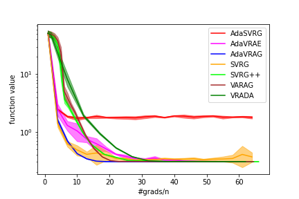
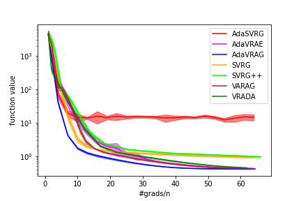
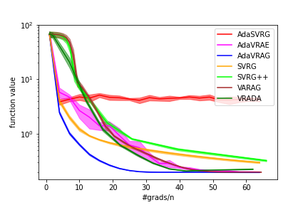
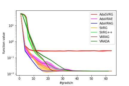
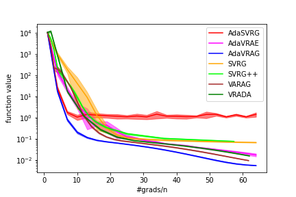
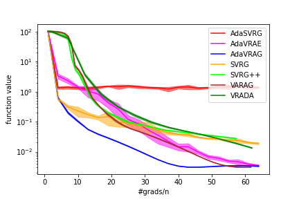
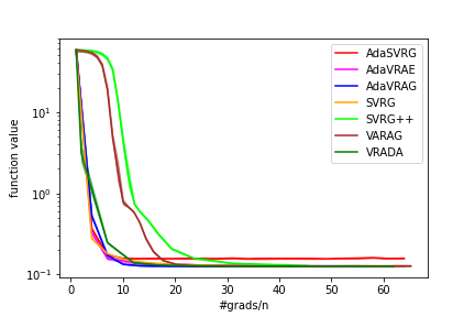
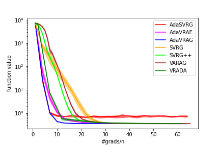
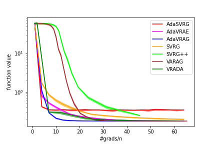
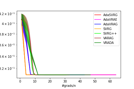
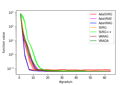
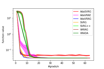
In this section we demonstrate the performances of AdaVRAG and AdaVRAE in comparison with the existing standard and adaptive VR methods. We use the experimental setup and the code base of [12].

Datasets and loss functions: We experiment with binary classification on four standard LIBSVM datasets: a1a, mushrooms, w8a and phishing [7]. For each dataset, we show the results for three different objective functions: logistic, squared and huber loss. Following the setting in [12] we add a $\ell_{2}$-regularization term to the loss function, with regularization set to $1/n$.

Constraint: In all experiments, we evaluate the algorithms under a ball constraint. That is, the domain of each problem in our experiment is a ball of radius $R=100$ around the initial point, which means for every algorithm, in the update step, we need to do a projection onto this ball.

Algorithms and hyperparameter selection: We compare AdaVRAE and AdaVRAG with the common VR algorithms: SVRG [18], $\text{SVRG}^{++}$[4], VARAG [22], VRADA [39], and AdaSVRG [12] (in the experiment the multi-stage variant performs worse than the fixed-sized inner loop variant, and we omit it from the plots). Among these, only AdaSVRG is an adaptive VR method, which does not require parameter tuning. For the non-adaptive methods we chose the step size (or equivalently, the inverse of the smoothness parameter ($1/\beta$) for VRADA) via hyperparameter search over $\left\{0.01,0.05,0.1,0.5,1,5,10,100\right\}$. For each experiment, we used the choice that led to the best performance, and we report the parameters used in Table 2. The adaptive methods — AdaSVRG, AdaVRAE, AdaVRAG — do not require any hyperparameter tuning and we set their parameters as prescribed by the theoretical analysis. For AdaSVRG, we used $\eta=D/\sqrt{2}=\sqrt{2}R$ as recommended in the original paper. For AdaVRAE and AdaVRAG, we used $\gamma=0.01$ and $\eta=D/2=R$.

Implementation and initialization: For all algorithms, in the inner loop, we use a random permutation to select a function. We also fix the batch size to $1$ in all cases to match the theoretical setting. We initialize $u^{(0)}$ to be a random point in $[0,10]^{d}$ where each dimension is uniformly chosen in $[0,10]$. Each experiment is repeated five times with different initial point, which is kept the same across all algorithms.

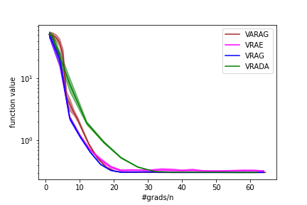
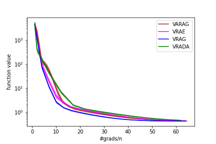
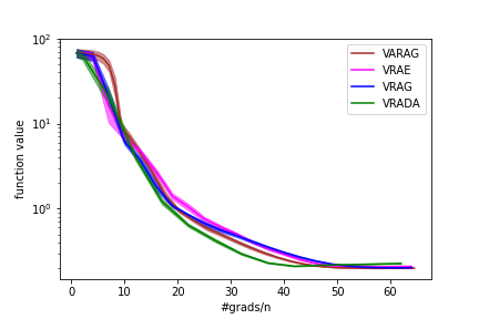
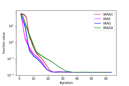
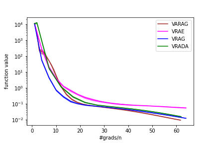
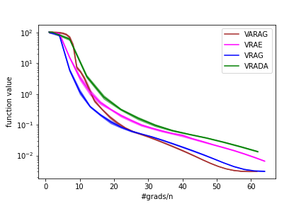
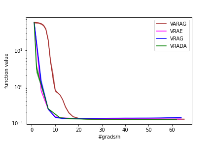
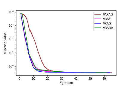
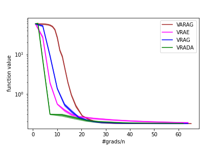
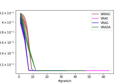
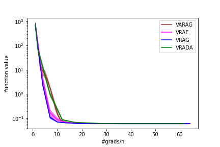
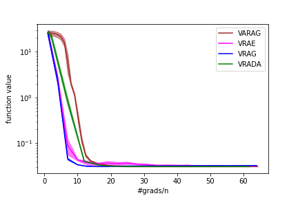
Results: The results are shown in Figures 1, 2, 3, 4. For each experiment, we plot the mean value and 95% confidence interval of the training objective against the number of gradient evaluations normalized by the number of examples.

Discussion: We observe that, in all experiments, AdaVRAG consistently performs competitively with all methods and generally have the best performances. The non-accelerated methods in general converge more slowly compared with accelerated methods, especially in the later epochs. In some cases, VARAG suffers from a slow convergence rate in the first phase. This is possibly due to the fact that it sets to $1/2$ the coefficient for the checkpoint in the first phase. VRADA sometimes exhibits similar behavior but to a lesser extent. In AdaVRAG and AdaVRAE, the coefficient for the checkpoint is set to be small in the beginning and gradually increased over time when the quality of the checkpoint is improved. The other adaptive method, AdaSVRG, exhibits slow convergence in many cases. One reason might be that AdaSVRG resets the step size in every epoch and, in later epochs, the step size may be too large for the algorithm to converge. In contrast, AdaVRAG and AdaVRAE use cumulative step sizes.

Appendix A Analysis of algorithm 1

In this section, we analyze Algorithm 1 and prove the following convergence guarantee:

Theorem A.1 (Convergence of AdaVRAE).

Define $s_{0}=\left\lceil\log_{2}\log_{2}4n\right\rceil$, $c=\frac{3}{2}$. If we choose parameters as follows

$$a^{(s)} =\begin{cases}(4n)^{-0.5^{s}}&1\leq s\leq s_{0}\\ \frac{s-s_{0}-1+c}{2c}&s_{0}<s\end{cases},$$

$$T_{s} =n,$$

$$A_{T_{0}}^{(0)} =\frac{5}{4}.$$

Assuming $\mathcal{X}$ is a compact convex set with diameter $D$, the number of individual gradient evaluations to achieve a solution $u^{(S)}$ such that $\mathbb{E}\left[F(u^{(S)})-F(x^{*})\right]\leq\epsilon$ for Algorithm 1 is

$$\#grads =\begin{cases}\mathcal{O}\text{$\left(n\log\log\frac{V}{\epsilon}\right)$}&\mbox{if }\epsilon\geq\frac{V}{n}\\ \mathcal{O}\left(n\log\log n+\sqrt{\frac{Vn}{\epsilon}}\right)&\mbox{if }\epsilon<\frac{V}{n}\end{cases}$$

where $V=\frac{5}{2}\left(F(u^{(0)})-F(x^{*})\right)+\text{$\gamma$}\left\|u^{(0)}-x^{*}\right\|^{2}+\frac{16\beta\left(D^{4}+2\eta^{4}\right)}{\eta^{2}}$.

To start with, we state and prove the following variance reduction lemma commonly used in accelerated methods:

Lemma A.2.

(Variance Reduction) Let $i\sim\mathrm{Uniform}([n])$ and $g=\nabla f_{i}(x)-\nabla f_{i}(u)+\nabla f(u)$ be an estimate of the gradient of $f$ at $x$. We have

$$\mathbb{E}_{i}\left[\left\|g-\nabla f(x)\right\|^{2}\right]\leq 2\beta\left(f(u)-f(x)-\left\langle\nabla f(x),u-x\right\rangle\right).$$

Proof.

By the definition of $g$,

$$\mathbb{E}_{i}\left[\left\|g-\nabla f(x)\right\|^{2}\right] =\mathbb{E}_{i}\left[\left\|\nabla f_{i}(x)-\nabla f_{i}(u)+\nabla f(u)-\nabla f(x)\right\|^{2}\right]$$

$$\overset{(a)}{\leq}\mathbb{E}_{i}\left[\left\|\nabla f_{i}(u)-\nabla f_{i}(x)\right\|^{2}\right]$$

$$\overset{(b)}{\leq}\mathbb{E}_{i}\left[2\beta\left(f_{i}(u)-f_{i}(x)-\left\langle\nabla f_{i}(x),u-x\right\rangle\right)\right]$$

$$\overset{(c)}{=}2\beta\left(f(u)-f(x)-\left\langle\nabla f(x),u-x\right\rangle\right),$$

where $(a)$ is because $\mathbb{E}_{i}\left[\nabla f_{i}(u)-\nabla f_{i}(x)\right]=\nabla f(u)-\nabla f(x)$ and $\mathbb{E}\left[\left\|X-\mathbb{E}\left[X\right]\right\|^{2}\right]\leq\mathbb{E}\left[\left\|X\right\|^{2}\right]$, $(b)$ is by the convexity and $\beta$-smoothness of $f_{i}$, $(c)$ is by $i\sim\mathrm{Uniform}([n])$ and the definition of $f$. ∎

A.1 Single iteration progress

We first analyze the progress in function value made in a single iteration of an epoch. The analysis follows the standard method as in [14]; however, we need to pay attention to the extra term for the checkpoint that appears in the convex combination for $\overline{x}_{t}^{(s)}$. We start off by the following observation

Lemma A.3.

For any $s\geq 1$ and $t\in\left[T_{s}\right]$,

$$\overline{x}_{t}^{(s)}-\overline{x}_{t-1}^{(s)}=\frac{a^{(s)}}{A_{t-1}^{(s)}}\left(x_{t}^{(s)}-\overline{x}_{t}^{(s)}\right)+\frac{\left(a^{(s)}\right)^{2}}{A_{t-1}^{(s)}}\left(u^{(s-1)}-\overline{x}_{t}^{(s)}\right).$$

Proof.

We note that the definition $\overline{x}_{t}^{(s)}=\frac{1}{A_{t}^{(s)}}\left(A_{t-1}^{(s)}\overline{x}_{t-1}^{(s)}+a^{(s)}x_{t}^{(s)}+\left(a^{(s)}\right)^{2}u^{(s-1)}\right)$ implies

$$A_{t}^{(s)}\overline{x}_{t}^{(s)} =A_{t-1}^{(s)}\overline{x}_{t-1}^{(s)}+a^{(s)}x_{t}^{(s)}+\left(a^{(s)}\right)^{2}u^{(s-1)}$$

$$\overset{(a)}{\Leftrightarrow}A_{t-1}^{(s)}(\overline{x}_{t}^{(s)}-\overline{x}_{t-1}^{(s)}) =a^{(s)}(x_{t}^{(s)}-\overline{x}_{t}^{(s)})+\left(a^{(s)}\right)^{2}(u^{(s-1)}-\overline{x}_{t}^{(s)})$$

$$\Leftrightarrow\overline{x}_{t}^{(s)}-\overline{x}_{t-1}^{(s)} =\frac{a^{(s)}}{A_{t-1}^{(s)}}\left(x_{t}^{(s)}-\overline{x}_{t}^{(s)}\right)+\frac{\left(a^{(s)}\right)^{2}}{A_{t-1}^{(s)}}\left(u^{(s-1)}-\overline{x}_{t}^{(s)}\right),$$

where $(a)$ is by $A_{t}^{(s)}=A_{t-1}^{(s)}+a^{(s)}+\left(a^{(s)}\right)^{2}$. ∎

Next, we bound the function progress in a single epoch via the stochastic regret. Note that, this lemma is somewhat weaker than we would desire, due to the appearance the coefficient of the checkpoint, making the LHS not immediately telescope. We will account for this factor later in the analysis.

Lemma A.4.

For all epochs $s\geq 1$ and all iterations $t\in\left[T_{s}\right]$

$$\mathbb{E}\left[\left(A_{t}^{(s)}-\left(a^{(s)}\right)^{2}\right)\left(F(\overline{x}_{t}^{(s)})-F(x^{*})\right)-A_{t-1}^{(s)}\left(F(\overline{x}_{t-1}^{(s)})-F(x^{*})\right)\right]$$

$$\leq \mathbb{E}\left[a^{(s)}\underbrace{\left\langle g_{t}^{(s)},x_{t}^{(s)}-x^{*}\right\rangle}_{\text{stochastic regret}}+\left(a^{(s)}\right)^{2}\left\langle\nabla f(\overline{x}_{t}^{(s)}),u^{(s-1)}-\overline{x}_{t}^{(s)}\right\rangle\right]$$

$$-\mathbb{E}\left[\frac{A_{t-1}^{(s)}}{2\beta}\left\|\nabla f(\overline{x}_{t}^{(s)})-\nabla f(\overline{x}_{t-1}^{(s)})\right\|^{2}\right]$$

$$+\mathbb{E}\left[\left(A_{t}^{(s)}-\left(a^{(s)}\right)^{2}\right)\left(h(\overline{x}_{t}^{(s)})-h(x^{*})\right)-A_{t-1}^{(s)}\left(h(\overline{x}_{t-1}^{(s)})-h(x^{*})\right)\right].$$

Proof.

Using the observation in Lemma A.3, we have

$$F(\overline{x}_{t}^{(s)})-F(\overline{x}_{t-1}^{(s)})$$

$$= f(\overline{x}_{t}^{(s)})-f(\overline{x}_{t-1}^{(s)})+h(\overline{x}_{t}^{(s)})-h(\overline{x}_{t-1}^{(s)})$$

$$\stackrel{{\scriptstyle(a)}}{{\leq}} \left\langle\nabla f(\overline{x}_{t}^{(s)}),\overline{x}_{t}^{(s)}-\overline{x}_{t-1}^{(s)}\right\rangle-\frac{1}{2\beta}\left\|\nabla f(\overline{x}_{t}^{(s)})-\nabla f(\overline{x}_{t-1}^{(s)})\right\|^{2}+h(\overline{x}_{t}^{(s)})-h(\overline{x}_{t-1}^{(s)})$$

$$\stackrel{{\scriptstyle(b)}}{{=}} \frac{a^{(s)}}{A_{t-1}}\left\langle\nabla f(\overline{x}_{t}^{(s)}),x_{t}^{(s)}-\overline{x}_{t}^{(s)}\right\rangle+\frac{\left(a^{(s)}\right)^{2}}{A_{t-1}^{(s)}}\left\langle\nabla f(\overline{x}_{t}^{(s)}),u^{(s-1)}-\overline{x}_{t}^{(s)}\right\rangle$$

$$-\frac{1}{2\beta}\left\|\nabla f(\overline{x}_{t}^{(s)})-\nabla f(\overline{x}_{t-1}^{(s)})\right\|^{2}+h(\overline{x}_{t}^{(s)})-h(\overline{x}_{t-1}^{(s)})$$

where $(a)$ is due to the smoothness of $f$ and $(b)$ comes from Lemma A.3. By the convexity of $f$, we also have

$$F(\overline{x}_{t}^{(s)})-F(x^{*})$$

$$= f(\overline{x}_{t}^{(s)})-f(x^{*})+h(\overline{x}_{t}^{(s)})-h(x^{*})$$

$$\leq \left\langle\nabla f(\overline{x}_{t}^{(s)}),\overline{x}_{t}^{(s)}-x^{*}\right\rangle+h(\overline{x}_{t}^{(s)})-h(x^{*})$$

We combine the two inequalities and obtain

$$A_{t-1}^{(s)}\left(F(\overline{x}_{t}^{(s)})-F(\overline{x}_{t-1}^{(s)})\right)+a^{(s)}\left(F(\overline{x}_{t}^{(s)})-F(x^{*})\right)$$

$$\leq a^{(s)}\left\langle\nabla f(\overline{x}_{t}^{(s)}),x_{t}^{(s)}-x^{*}\right\rangle+\left(a^{(s)}\right)^{2}\left\langle\nabla f(\overline{x}_{t}^{(s)}),u^{(s-1)}-\overline{x}_{t}^{(s)}\right\rangle$$

$$-\frac{A_{t-1}}{2\beta}\left\|\nabla f(\overline{x}_{t}^{(s)})-\nabla f(\overline{x}_{t-1}^{(s)})\right\|^{2}$$

$$+A_{t-1}^{(s)}\left(h(\overline{x}_{t}^{(s)})-h(\overline{x}_{t-1}^{(s)})\right)+a^{(s)}\left(h(\overline{x}_{t}^{(s)})-h(x^{*})\right)$$

$$= a^{(s)}\left\langle g_{t}^{(s)},x_{t}^{(s)}-x^{*}\right\rangle+\left(a^{(s)}\right)^{2}\left\langle\nabla f(\overline{x}_{t}^{(s)}),u^{(s-1)}-\overline{x}_{t}^{(s)}\right\rangle$$

$$+a^{(s)}\left\langle\nabla f(\overline{x}_{t}^{(s)})-g_{t}^{(s)},x_{t}^{(s)}-x^{*}\right\rangle-\frac{A_{t-1}^{(s)}}{2\beta}\left\|\nabla f(\overline{x}_{t}^{(s)})-\nabla f(\overline{x}_{t-1}^{(s)})\right\|^{2}$$

$$+A_{t-1}^{(s)}\left(h(\overline{x}_{t}^{(s)})-h(\overline{x}_{t-1}^{(s)})\right)+a^{(s)}\left(h(\overline{x}_{t}^{(s)})-h(x^{*})\right).$$

Note that we can rearrange the terms

$$A_{t-1}^{(s)}\left(F(\overline{x}_{t}^{(s)})-F(\overline{x}_{t-1}^{(s)})\right)+a^{(s)}\left(F(\overline{x}_{t}^{(s)})-F(x^{*})\right)$$

$$= \left(A_{t}^{(s)}-\left(a^{(s)}\right)^{2}\right)\left(F(\overline{x}_{t}^{(s)})-F(x^{*})\right)-A_{t-1}^{(s)}\left(F(\overline{x}_{t-1}^{(s)})-F(x^{*})\right),$$

$$A_{t-1}^{(s)}\left(h(\overline{x}_{t}^{(s)})-h(\overline{x}_{t-1}^{(s)})\right)+a^{(s)}\left(h(\overline{x}_{t}^{(s)})-h(x^{*})\right)$$

$$= \left(A_{t}^{(s)}-\left(a^{(s)}\right)^{2}\right)\left(h(\overline{x}_{t}^{(s)})-h(x^{*})\right)-A_{t-1}^{(s)}\left(h(\overline{x}_{t-1}^{(s)})-h(x^{*})\right).$$

Thus we obtain

$$\left(A_{t}^{(s)}-\left(a^{(s)}\right)^{2}\right)\left(F(\overline{x}_{t}^{(s)})-F(x^{*})\right)-A_{t-1}^{(s)}\left(F(\overline{x}_{t-1}^{(s)})-F(x^{*})\right)$$

$$\leq a^{(s)}\left\langle g_{t}^{(s)},x_{t}^{(s)}-x^{*}\right\rangle+\left(a^{(s)}\right)^{2}\left\langle\nabla f(\overline{x}_{t}^{(s)}),u^{(s-1)}-\overline{x}_{t}^{(s)}\right\rangle$$

$$+a^{(s)}\left\langle\nabla f(\overline{x}_{t}^{(s)})-g_{t}^{(s)},x_{t}^{(s)}-x^{*}\right\rangle-\frac{A_{t-1}^{(s)}}{2\beta}\left\|\nabla f(\overline{x}_{t}^{(s)})-\nabla f(\overline{x}_{t-1}^{(s)})\right\|^{2}$$

$$+\left(A_{t}^{(s)}-\left(a^{(s)}\right)^{2}\right)\left(h(\overline{x}_{t}^{(s)})-h(x^{*})\right)-A_{t-1}^{(s)}\left(h(\overline{x}_{t-1}^{(s)})-h(x^{*})\right).$$ (3)

Observe that for $t<T_{s}$

$$\mathbb{E}\left[a^{(s)}\left\langle\nabla f(\overline{x}_{t}^{(s)})-g_{t}^{(s)},x_{t}^{(s)}-x^{*}\right\rangle\right] =\mathbb{E}\left[\mathbb{E}_{i_{t}^{(s)}}\left[a^{(s)}\left\langle\nabla f(\overline{x}_{t}^{(s)})-g_{t}^{(s)},x_{t}^{(s)}-x^{*}\right\rangle\right]\right]$$

$$=0.$$

and for $t=T_{s},$we have $\nabla f(\overline{x}_{t}^{(s)})=g_{t}^{(s)}$ thus $\mathbb{E}\left[a^{(s)}\left\langle\nabla f(\overline{x}_{t}^{(s)})-g_{t}^{(s)},x_{t}^{(s)}-x^{*}\right\rangle\right]=0$. By taking expectations w.r.t. both sides of (3), we get

$$\mathbb{E}\left[\left(A_{t}^{(s)}-\left(a^{(s)}\right)^{2}\right)\left(F(\overline{x}_{t}^{(s)})-F(x^{*})\right)-A_{t-1}^{(s)}\left(F(\overline{x}_{t-1}^{(s)})-F(x^{*})\right)\right]$$

$$\leq \mathbb{E}\left[a^{(s)}\left\langle g_{t}^{(s)},x_{t}^{(s)}-x^{*}\right\rangle+\left(a^{(s)}\right)^{2}\left\langle\nabla f(\overline{x}_{t}^{(s)}),u^{(s-1)}-\overline{x}_{t}^{(s)}\right\rangle\right]$$

$$-\mathbb{E}\left[\frac{A_{t-1}^{(s)}}{2\beta}\left\|\nabla f(\overline{x}_{t}^{(s)})-\nabla f(\overline{x}_{t-1}^{(s)})\right\|^{2}\right]$$

$$+\mathbb{E}\left[\left(A_{t}^{(s)}-\left(a^{(s)}\right)^{2}\right)\left(h(\overline{x}_{t}^{(s)})-h(x^{*})\right)-A_{t-1}^{(s)}\left(h(\overline{x}_{t-1}^{(s)})-h(x^{*})\right)\right].$$

∎

To analyze the stochastic regret, we split the inner product as follows

$$\left\langle g_{t}^{(s)},x_{t}^{(s)}-x^{*}\right\rangle =\left\langle g_{t}^{(s)},z_{t}^{(s)}-x^{*}\right\rangle+\left\langle g_{t}^{(s)}-g_{t-1}^{(s)},x_{t}^{(s)}-z_{t}^{(s)}\right\rangle+\left\langle g_{t-1}^{(s)},x_{t}^{(s)}-z_{t}^{(s)}\right\rangle.$$

For each term we give a bound as stated in Lemma A.5.

Lemma A.5.

For any $s\geq 1$ all iterations $t\in\left[T_{s}\right]$, we have

$$a^{(s)}\left\langle g_{t-1}^{(s)},x_{t}^{(s)}-z_{t}^{(s)}\right\rangle \leq\frac{\gamma_{t-1}^{(s)}}{2}\left\|z_{t-1}^{(s)}-z_{t}^{(s)}\right\|^{2}-\frac{\gamma_{t-1}^{(s)}}{2}\left\|z_{t-1}^{(s)}-x_{t}^{(s)}\right\|^{2}-\frac{\gamma_{t-1}^{(s)}}{2}\left\|x_{t}^{(s)}-z_{t}^{(s)}\right\|^{2}$$

$$\quad+a^{(s)}\left(h(z_{t}^{(s)})-h(x_{t}^{(s)})\right).$$

$$a^{(s)}\left\langle g_{t}^{(s)},z_{t}^{(s)}-x^{*}\right\rangle \leq\frac{\gamma_{t}^{(s)}-\gamma_{t-1}^{(s)}}{2}\left\|x_{t}^{(s)}-x^{*}\right\|^{2}+\frac{\gamma_{t-1}^{(s)}}{2}\left\|z_{t-1}^{(s)}-x^{*}\right\|^{2}-\frac{\gamma_{t}^{(s)}}{2}\left\|z_{t}^{(s)}-x^{*}\right\|^{2}$$

$$\quad-\frac{\gamma_{t-1}^{(s)}}{2}\left\|z_{t}^{(s)}-z_{t-1}^{(s)}\right\|^{2}-\frac{\gamma_{t}^{(s)}-\gamma_{t-1}^{(s)}}{2}\left\|x_{t}^{(s)}-z_{t}^{(s)}\right\|^{2}$$

$$\quad+a^{(s)}\left(h(x^{*})-h(z_{t}^{(s)})\right).$$

$$a^{(s)}\left\langle g_{t}^{(s)}-g_{t-1}^{(s)},x_{t}^{(s)}-z_{t}^{(s)}\right\rangle \leq\frac{\left(a^{(s)}\right)^{2}}{2\gamma_{t}^{(s)}}\left\|g_{t}^{(s)}-g_{t-1}^{(s)}\right\|^{2}+\frac{\gamma_{t}^{(s)}}{2}\left\|x_{t}^{(s)}-z_{t}^{(s)}\right\|^{2}.$$

Proof.

Since $x_{t}^{(s)}=\arg\min_{x\in\mathcal{X}}\left\{a^{(s)}\left\langle g_{t-1}^{(s)},x\right\rangle+a^{(s)}h(x)+\frac{\gamma_{t-1}^{(s)}}{2}\left\|x-z_{t-1}^{(s)}\right\|^{2}\right\}$, by the optimality condition of $x_{t}^{(s)}$, we have

$$\left\langle a^{(s)}g_{t-1}^{(s)}+a^{(s)}h^{\prime}(x_{t}^{(s)})+\gamma_{t-1}^{(s)}\left(x_{t}^{(s)}-z_{t-1}^{(s)}\right),x_{t}^{(s)}-z_{t}^{(s)}\right\rangle \leq 0,$$

where $h^{\prime}(x_{t}^{(s)})\in\partial h(x_{t}^{(s)})$ is a subgradient of $h$ at $x_{t}^{(s)}$. We rearrange the above inequality and obtain

$$a^{(s)}\left\langle g_{t-1}^{(s)},x_{t}^{(s)}-z_{t}^{(s)}\right\rangle \leq\gamma_{t-1}^{(s)}\left\langle x_{t}^{(s)}-z_{t-1}^{(s)},z_{t}^{(s)}-x_{t}^{(s)}\right\rangle+a^{(s)}\left\langle h^{\prime}(x_{t}^{(s)}),z_{t}^{(s)}-x_{t}^{(s)}\right\rangle$$

$$\overset{(a)}{\leq}\gamma_{t-1}^{(s)}\left\langle x_{t}^{(s)}-z_{t-1}^{(s)},z_{t}^{(s)}-x_{t}^{(s)}\right\rangle+a^{(s)}\left(h(z_{t}^{(s)})-h(x_{t}^{(s)})\right)$$

$$\overset{(b)}{=}\frac{\gamma_{t-1}^{(s)}}{2}\left\|z_{t-1}^{(s)}-z_{t}^{(s)}\right\|^{2}-\frac{\gamma_{t-1}^{(s)}}{2}\left\|z_{t-1}^{(s)}-x_{t}^{(s)}\right\|^{2}-\frac{\gamma_{t-1}^{(s)}}{2}\left\|x_{t}^{(s)}-z_{t}^{(s)}\right\|^{2}$$

$$\quad+a^{(s)}\left(h(z_{t}^{(s)})-h(x_{t}^{(s)})\right),$$

where $(a)$ follows from the convexity of $h$ and the fact that $h^{\prime}(x_{t}^{(s)})\in\partial h(x_{t}^{(s)})$, and $(b)$ is due to the identity $\langle a,b\rangle=\frac{1}{2}\left(\left\|a+b\right\|^{2}-\left\|a\right\|^{2}-\left\|b\right\|^{2}\right)$.

Using the optimality condition of $z_{t}^{(s)}$, we have

$$\left\langle a^{(s)}g_{t}^{(s)}+a^{(s)}h^{\prime}(z_{t}^{(s)})+\gamma_{t-1}^{(s)}\left(z_{t}^{(s)}-z_{t-1}^{(s)}\right)+\left(\gamma_{t}^{(s)}-\gamma_{t-1}^{(s)}\right)\left(z_{t}^{(s)}-x_{t}^{(s)}\right),z_{t}^{(s)}-x^{*}\right\rangle \leq 0$$

where $h^{\prime}(z_{t}^{(s)})\in\partial h(z_{t}^{(s)})$ is a subgradient of $h$ at $z_{t}^{(s)}$. We rearrange the above inequality and obtain

$$a^{(s)}\left\langle g_{t}^{(s)},z_{t}^{(s)}-x^{*}\right\rangle \leq\gamma_{t-1}^{(s)}\left\langle z_{t}^{(s)}-z_{t-1}^{(s)},x^{*}-z_{t}^{(s)}\right\rangle+\left(\gamma_{t}^{(s)}-\gamma_{t-1}^{(s)}\right)\left\langle z_{t}^{(s)}-x_{t}^{(s)},x^{*}-z_{t}^{(s)}\right\rangle$$

$$\quad+a^{(s)}\left\langle h^{\prime}(z_{t}^{(s)}),x^{*}-z_{t}^{(s)}\right\rangle$$

$$\overset{(c)}{\leq}\gamma_{t-1}^{(s)}\left\langle z_{t}^{(s)}-z_{t-1}^{(s)},x^{*}-z_{t}^{(s)}\right\rangle+\left(\gamma_{t}^{(s)}-\gamma_{t-1}^{(s)}\right)\left\langle z_{t}^{(s)}-x_{t}^{(s)},x^{*}-z_{t}^{(s)}\right\rangle$$

$$\quad+a^{(s)}\left(h(x^{*})-h(z_{t}^{(s)})\right)$$

$$\overset{(d)}{=}\frac{\gamma_{t-1}^{(s)}}{2}\left[\left\|z_{t-1}^{(s)}-x^{*}\right\|^{2}-\left\|z_{t}^{(s)}-x^{*}\right\|^{2}-\left\|z_{t}^{(s)}-z_{t-1}^{(s)}\right\|^{2}\right]$$

$$\quad+\frac{\gamma_{t}^{(s)}-\gamma_{t-1}^{(s)}}{2}\left[\left\|x_{t}^{(s)}-x^{*}\right\|^{2}-\left\|z_{t}^{(s)}-x^{*}\right\|^{2}-\left\|x_{t}^{(s)}-z_{t}^{(s)}\right\|^{2}\right]$$

$$\quad+a^{(s)}\left(h(x^{*})-h(z_{t}^{(s)})\right)$$

$$=\frac{\gamma_{t}^{(s)}-\gamma_{t-1}^{(s)}}{2}\left\|x_{t}^{(s)}-x^{*}\right\|^{2}+\frac{\gamma_{t-1}^{(s)}}{2}\left\|z_{t-1}^{(s)}-x^{*}\right\|^{2}-\frac{\gamma_{t}^{(s)}}{2}\left\|z_{t}^{(s)}-x^{*}\right\|^{2}$$

$$\quad-\frac{\gamma_{t-1}^{(s)}}{2}\left\|z_{t}^{(s)}-z_{t-1}^{(s)}\right\|^{2}-\frac{\gamma_{t}^{(s)}-\gamma_{t-1}^{(s)}}{2}\left\|x_{t}^{(s)}-z_{t}^{(s)}\right\|^{2}$$

$$\quad+a^{(s)}\left(h(x)-h(z_{t}^{(s)})\right),$$

where $(c)$ follows from the convexity of $h$ and the fact that $h^{\prime}(z_{t}^{(s)})\in\partial h(z_{t}^{(s)})$, and $(d)$ is due to the identity $\langle a,b\rangle=\frac{1}{2}\left(\left\|a+b\right\|^{2}-\left\|a\right\|^{2}-\left\|b\right\|^{2}\right)$.

For the third inequality, we have

$$a^{(s)}\left\langle g_{t}^{(s)}-g_{t-1}^{(s)},x_{t}^{(s)}-z_{t}^{(s)}\right\rangle \overset{(e)}{\leq}a^{(s)}\left\|g_{t}^{(s)}-g_{t-1}^{(s)}\right\|\left\|x_{t}^{(s)}-z_{t}^{(s)}\right\|$$

$$\overset{(f)}{\leq}\frac{\left(a^{(s)}\right)^{2}}{2\gamma_{t}^{(s)}}\left\|g_{t}^{(s)}-g_{t-1}^{(s)}\right\|^{2}+\frac{\gamma_{t}^{(s)}}{2}\left\|x_{t}^{(s)}-z_{t}^{(s)}\right\|^{2}.$$

where $(e)$ is by the Cauchy–Schwarz inequality, $(f)$ is by Young’s inequality. ∎

With above results, we obtain the descent lemma for one iteration. A key idea to remove $\left(a^{(s)}\right)^{2}$ from the coefficient of $\left(F(\overline{x}_{t}^{(s)})-F(x^{*})\right)$ is to split the term $\frac{\left(a^{(s)}\right)^{2}}{2\gamma_{t}^{(s)}}\left\|g_{t}^{(s)}-g_{t-1}^{(s)}\right\|^{2}$ into $\left(\frac{\left(a^{(s)}\right)^{2}}{2\gamma_{t}^{(s)}}-\frac{\left(a^{(s)}\right)^{2}}{16\beta}\right)\left\|g_{t}^{(s)}-g_{t-1}^{(s)}\right\|^{2}+\frac{\left(a^{(s)}\right)^{2}}{16\beta}\left\|g_{t}^{(s)}-g_{t-1}^{(s)}\right\|^{2}$ and apply the VR lemma for the second term.

Lemma A.6.

For all epochs $s\geq 1$ and all iterations $t\in\left[T_{s}\right]$, we have

$$\mathbb{E}\left[\left(A_{t}^{(s)}-\left(a^{(s)}\right)^{2}\right)\left(F(\overline{x}_{t}^{(s)})-F(x^{*})\right)-A_{t-1}^{(s)}\left(F(\overline{x}_{t-1}^{(s)})-F(x^{*})\right)\right]$$

$$\leq \mathbb{E}\left[\frac{\gamma_{t-1}^{(s)}}{2}\left\|z_{t-1}^{(s)}-x^{*}\right\|^{2}-\frac{\gamma_{t}^{(s)}}{2}\left\|z_{t}^{(s)}-x^{*}\right\|^{2}+\frac{\gamma_{t}^{(s)}-\gamma_{t-1}^{(s)}}{2}\left\|x_{t}^{(s)}-x^{*}\right\|^{2}\right]$$

$$+\mathbb{E}\left[\left(a^{(s)}\right)^{2}\left\langle\nabla f(\overline{x}_{t}^{(s)}),u^{(s-1)}-\overline{x}_{t}^{(s)}\right\rangle\right]$$

$$+\mathbb{E}\left[\frac{\left(a^{(s)}\right)^{2}}{2}\left(f(u^{(s-1)})-f(\overline{x}_{t}^{(s)})-\left\langle\nabla f(\overline{x}_{t}^{(s)}),u^{(s-1)}-\overline{x}_{t}^{(s)}\right\rangle\right)\right]$$

$$+\mathbb{E}\left[\frac{\left(a^{(s)}\right)^{2}}{2}\left(f(u^{(s-1)})-f(\overline{x}_{t-1}^{(s)})-\left\langle\nabla f(\overline{x}_{t-1}^{(s)}),u^{(s-1)}-\overline{x}_{t-1}^{(s)}\right\rangle\right)\right]$$

$$+\mathbb{E}\left[\left(\frac{\left(a^{(s)}\right)^{2}}{2\gamma_{t}^{(s)}}-\frac{\left(a^{(s)}\right)^{2}}{16\beta}\right)\left\|g_{t}^{(s)}-g_{t-1}^{(s)}\right\|^{2}+\left(\frac{\left(a^{(s)}\right)^{2}}{8\beta}-\frac{A_{t-1}^{(s)}}{2\beta}\right)\left\|\nabla f(\overline{x}_{t}^{(s)})-\nabla f(\overline{x}_{t-1}^{(s)})\right\|^{2}\right]$$

$$+\mathbb{E}\left[\left(a^{(s)}\right)^{2}\left(h(u^{(s-1)})-h(\overline{x}_{t}^{(s)})\right)\right].$$

Proof.

By Lemma A.5, we can bound $a^{(s)}\left\langle g_{t}^{(s)},x_{t}^{(s)}-x^{*}\right\rangle$ as follows

$$a^{(s)}\left\langle g_{t}^{(s)},x_{t}^{(s)}-x^{*}\right\rangle \leq\frac{\gamma_{t-1}^{(s)}}{2}\left\|z_{t-1}^{(s)}-x^{*}\right\|^{2}-\frac{\gamma_{t}^{(s)}}{2}\left\|z_{t}^{(s)}-x^{*}\right\|^{2}+\frac{\gamma_{t}^{(s)}-\gamma_{t-1}^{(s)}}{2}\left\|x_{t}^{(s)}-x^{*}\right\|^{2}-\frac{\gamma_{t-1}^{(s)}}{2}\left\|z_{t-1}^{(s)}-x_{t}^{(s)}\right\|^{2}$$

$$\quad+a^{(s)}\left(h(x^{*})-h(x_{t}^{(s)})\right)+\frac{\left(a^{(s)}\right)^{2}}{2\gamma_{t}^{(s)}}\left\|g_{t}^{(s)}-g_{t-1}^{(s)}\right\|^{2}.$$

$$\leq\frac{\gamma_{t-1}^{(s)}}{2}\left\|z_{t-1}^{(s)}-x^{*}\right\|^{2}-\frac{\gamma_{t}^{(s)}}{2}\left\|z_{t}^{(s)}-x^{*}\right\|^{2}+\frac{\gamma_{t}^{(s)}-\gamma_{t-1}^{(s)}}{2}\left\|x_{t}^{(s)}-x^{*}\right\|^{2}$$

$$\quad+a^{(s)}\left(h(x^{*})-h(x_{t}^{(s)})\right)+\frac{\left(a^{(s)}\right)^{2}}{2\gamma_{t}^{(s)}}\left\|g_{t}^{(s)}-g_{t-1}^{(s)}\right\|^{2}.$$

Combining the above result with Lemma A.4, we know

$$\mathbb{E}\left[\left(A_{t}^{(s)}-\left(a^{(s)}\right)^{2}\right)\left(F(\overline{x}_{t}^{(s)})-F(x^{*})\right)-A_{t-1}^{(s)}\left(F(\overline{x}_{t-1}^{(s)})-F(x^{*})\right)\right]$$

$$\leq \mathbb{E}\left[\frac{\gamma_{t-1}^{(s)}}{2}\left\|z_{t-1}^{(s)}-x^{*}\right\|^{2}-\frac{\gamma_{t}^{(s)}}{2}\left\|z_{t}^{(s)}-x^{*}\right\|^{2}+\frac{\gamma_{t}^{(s)}-\gamma_{t-1}^{(s)}}{2}\left\|x_{t}^{(s)}-x^{*}\right\|^{2}\right]$$

$$+\mathbb{E}\left[\left(a^{(s)}\right)^{2}\left\langle\nabla f(\overline{x}_{t}^{(s)}),u^{(s-1)}-\overline{x}_{t}^{(s)}\right\rangle\right]$$

$$+\mathbb{E}\left[\frac{\left(a^{(s)}\right)^{2}}{2\gamma_{t}^{(s)}}\left\|g_{t}^{(s)}-g_{t-1}^{(s)}\right\|^{2}-\frac{A_{t-1}^{(s)}}{2\beta}\left\|\nabla f(\overline{x}_{t}^{(s)})-\nabla f(\overline{x}_{t-1}^{(s)})\right\|^{2}\right]$$

$$+\mathbb{E}\left[\left(A_{t}^{(s)}-\left(a^{(s)}\right)^{2}\right)\left(h(\overline{x}_{t}^{(s)})-h(x^{*})\right)-A_{t-1}^{(s)}\left(h(\overline{x}_{t-1}^{(s)})-h(x^{*})\right)+a^{(s)}\left(h(x^{*})-h(x_{t}^{(s)})\right)\right].$$ (4)

Note that

$$\left(A_{t}^{(s)}-\left(a^{(s)}\right)^{2}\right)\left(h(\overline{x}_{t}^{(s)})-h(x^{*})\right)-A_{t-1}^{(s)}\left(h(\overline{x}_{t-1}^{(s)})-h(x^{*})\right)+a^{(s)}\left(h(x^{*})-h(x_{t}^{(s)})\right)$$

$$= \left(A_{t}^{(s)}-\left(a^{(s)}\right)^{2}\right)\left(h(\overline{x}_{t}^{(s)})-h(x^{*})\right)+\left(a^{(s)}\right)^{2}\left(h(u^{(s-1)})-h(x^{*})\right)$$

$$-\left(a^{(s)}\right)^{2}\left(h(u^{(s-1)})-h(x^{*})\right)-A_{t-1}^{(s)}\left(h(\overline{x}_{t-1}^{(s)})-h(x^{*})\right)-a^{(s)}\left(h(x_{t}^{(s)})-h(x^{*})\right)$$

$$\stackrel{{\scriptstyle(a)}}{{\leq}} \left(A_{t}^{(s)}-\left(a^{(s)}\right)^{2}\right)\left(h(\overline{x}_{t}^{(s)})-h(x^{*})\right)+\left(a^{(s)}\right)^{2}\left(h(u^{(s-1)})-h(x^{*})\right)$$

$$-A_{t}^{(s)}(h(\overline{x}_{t}^{(s)})-h(x^{*}))$$

$$= \left(a^{(s)}\right)^{2}\left(h(u^{(s-1)})-h(\overline{x}_{t}^{(s)})\right),$$ (5)

where $(a)$ is by the convexity of $h$ and $A_{t}^{(s)}=A_{t-1}^{(s)}+a^{(s)}+\left(a^{(s)}\right)^{2}$. Plugging in (5) into (4), we know

$$\mathbb{E}\left[\left(A_{t}^{(s)}-\left(a^{(s)}\right)^{2}\right)\left(F(\overline{x}_{t}^{(s)})-F(x^{*})\right)-A_{t-1}^{(s)}\left(F(\overline{x}_{t-1}^{(s)})-F(x^{*})\right)\right]$$

$$\leq \mathbb{E}\left[\frac{\gamma_{t-1}^{(s)}}{2}\left\|z_{t-1}^{(s)}-x^{*}\right\|^{2}-\frac{\gamma_{t}^{(s)}}{2}\left\|z_{t}^{(s)}-x^{*}\right\|^{2}+\frac{\gamma_{t}^{(s)}-\gamma_{t-1}^{(s)}}{2}\left\|x_{t}^{(s)}-x^{*}\right\|^{2}\right]$$

$$+\mathbb{E}\left[\left(a^{(s)}\right)^{2}\left\langle\nabla f(\overline{x}_{t}^{(s)}),u^{(s-1)}-\overline{x}_{t}^{(s)}\right\rangle\right]$$

$$+\mathbb{E}\left[\frac{\left(a^{(s)}\right)^{2}}{2\gamma_{t}^{(s)}}\left\|g_{t}^{(s)}-g_{t-1}^{(s)}\right\|^{2}-\frac{A_{t-1}^{(s)}}{2\beta}\left\|\nabla f(\overline{x}_{t}^{(s)})-\nabla f(\overline{x}_{t-1}^{(s)})\right\|^{2}\right]$$

$$+\mathbb{E}\left[\left(a^{(s)}\right)^{2}\left(h(u^{(s-1)})-h(\overline{x}_{t}^{(s)})\right)\right].$$

Now for $\mathbb{E}\left[\left\|g_{t}^{(s)}-g_{t-1}^{(s)}\right\|^{2}\right]$, when $1<t<T_{s}$, we have

$$\mathbb{E}\left[\left\|g_{t}^{(s)}-g_{t-1}^{(s)}\right\|^{2}\right] \leq\mathbb{E}\left[4\left\|\nabla f(\overline{x}_{t}^{(s)})-g_{t}^{(s)}\right\|^{2}+4\left\|\nabla f(\overline{x}_{t-1}^{(s)})-g_{t-1}^{(s)}\right\|^{2}\right]$$

$$\quad+\mathbb{E}\left[2\left\|\nabla f(\overline{x}_{t}^{(s)})-\nabla f(\overline{x}_{t-1}^{(s)})\right\|^{2}\right]$$

$$\overset{(b)}{\leq}\mathbb{E}\left[8\beta\left(f(u^{(s-1)})-f(\overline{x}_{t}^{(s)})-\left\langle\nabla f(\overline{x}_{t}^{(s)}),u^{(s-1)}-\overline{x}_{t}^{(s)}\right\rangle\right)\right]$$

$$\quad+\mathbb{E}\left[8\beta\left(f(u^{(s-1)})-f(\overline{x}_{t-1}^{(s)})-\left\langle\nabla f(\overline{x}_{t-1}^{(s)}),u^{(s-1)}-\overline{x}_{t-1}^{(s)}\right\rangle\right)\right]$$

$$\quad+\mathbb{E}\left[2\left\|\nabla f(\overline{x}_{t}^{(s)})-\nabla f(\overline{x}_{t-1}^{(s)})\right\|^{2}\right],$$ (6)

where $(b)$ is by Lemma A.2 for all $1<t<T_{s}$. When $t=1$, note that both $\left\|\nabla f(\overline{x}_{t-1}^{(s)})-g_{t-1}^{(s)}\right\|^{2}$ and $f(u^{(s-1)})-f(\overline{x}_{t-1}^{(s)})-\left\langle\nabla f(\overline{x}_{t-1}^{(s)}),u^{(s-1)}-\overline{x}_{t-1}^{(s)}\right\rangle$ are zero by our definition $\overline{x}_{0}^{(s)}=u^{(s-1)}$ and $\nabla f(\overline{x}_{0}^{(s)})=\nabla f(\overline{x}_{T_{s-1}}^{(s-1)})=g_{T_{s-1}}^{(s-1)}=g_{0}^{(s)}$, which means the above inequality is still true. When $t=T_{s}$, note that $\left\|\nabla f(\overline{x}_{t}^{(s)})-g_{t}^{(s)}\right\|^{2}=0$ and $f(u^{(s-1)})-f(\overline{x}_{t}^{(s)})-\left\langle\nabla f(\overline{x}_{t}^{(s)}),u^{(s-1)}-\overline{x}_{t}^{(s)}\right\rangle$ is always non-negative due to the convexity of $f$. So the above inequality also holds in this case. Now we conlclude the above inequality is right for $t\in\left[T_{s}\right]$.

Splitting $\frac{\left(a^{(s)}\right)^{2}}{2\gamma_{t}^{(s)}}\left\|g_{t}^{(s)}-g_{t-1}^{(s)}\right\|^{2}$ into $\left(\frac{\left(a^{(s)}\right)^{2}}{2\gamma_{t}^{(s)}}-\frac{\left(a^{(s)}\right)^{2}}{16\beta}\right)\left\|g_{t}^{(s)}-g_{t-1}^{(s)}\right\|^{2}+\frac{\left(a^{(s)}\right)^{2}}{16\beta}\left\|g_{t}^{(s)}-g_{t-1}^{(s)}\right\|^{2}$ and applying (6) to $\frac{\left(a^{(s)}\right)^{2}}{16\beta}\left\|g_{t}^{(s)}-g_{t-1}^{(s)}\right\|^{2}$, we have

$$\mathbb{E}\left[\left(A_{t}^{(s)}-\left(a^{(s)}\right)^{2}\right)\left(F(\overline{x}_{t}^{(s)})-F(x^{*})\right)-A_{t-1}^{(s)}\left(F(\overline{x}_{t-1}^{(s)})-F(x^{*})\right)\right]$$

$$\leq \mathbb{E}\left[\frac{\gamma_{t-1}^{(s)}}{2}\left\|z_{t-1}^{(s)}-x^{*}\right\|^{2}-\frac{\gamma_{t}^{(s)}}{2}\left\|z_{t}^{(s)}-x^{*}\right\|^{2}+\frac{\gamma_{t}^{(s)}-\gamma_{t-1}^{(s)}}{2}\left\|x_{t}^{(s)}-x^{*}\right\|^{2}\right]$$

$$+\mathbb{E}\left[\left(a^{(s)}\right)^{2}\left\langle\nabla f(\overline{x}_{t}^{(s)}),u^{(s-1)}-\overline{x}_{t}^{(s)}\right\rangle\right]$$

$$+\mathbb{E}\left[\frac{\left(a^{(s)}\right)^{2}}{2}\left(f(u^{(s-1)})-f(\overline{x}_{t}^{(s)})-\left\langle\nabla f(\overline{x}_{t}^{(s)}),u^{(s-1)}-\overline{x}_{t}^{(s)}\right\rangle\right)\right]$$

$$+\mathbb{E}\left[\frac{\left(a^{(s)}\right)^{2}}{2}\left(f(u^{(s-1)})-f(\overline{x}_{t-1}^{(s)})-\left\langle\nabla f(\overline{x}_{t-1}^{(s)}),u^{(s-1)}-\overline{x}_{t-1}^{(s)}\right\rangle\right)\right]$$

$$+\mathbb{E}\left[\left(\frac{\left(a^{(s)}\right)^{2}}{2\gamma_{t}^{(s)}}-\frac{\left(a^{(s)}\right)^{2}}{16\beta}\right)\left\|g_{t}^{(s)}-g_{t-1}^{(s)}\right\|^{2}+\left(\frac{\left(a^{(s)}\right)^{2}}{8\beta}-\frac{A_{t-1}^{(s)}}{2\beta}\right)\left\|\nabla f(\overline{x}_{t}^{(s)})-\nabla f(\overline{x}_{t-1}^{(s)})\right\|^{2}\right]$$

$$+\mathbb{E}\left[\left(a^{(s)}\right)^{2}\left(h(u^{(s-1)})-h(\overline{x}_{t}^{(s)})\right)\right].$$

∎

A.2 Single epoch progress and final output

Even though Lemma A.6 looks somewhat more convoluted, when we sum up over all iterations in one epoch, many terms are canceled out nicely and we obtain the following lemma that states the progress of the function value in one epoch. The trick is to set the value for each term at the end of one epoch equal to its value in the next one, with an exception for $A_{T_{s-1}}^{(s-1)}$. Due to the accumulation of the term $\left(F(u^{(s-1)})-F(x^{*})\right)$ throughout the epoch, we will set $A_{0}^{(s)}=A_{T_{s-1}}^{(s-1)}-T_{s}\left(a^{(s)}\right)^{2}$.

Lemma A.7.

For all epochs $s\geq 1$, if

$$\left(a^{(s)}\right)^{2} \leq 4A_{t-1}^{(s)},\forall t\in\left[T_{s}\right].$$

We have

$$\mathbb{E}\left[A_{T_{s}}^{(s)}\left(F(u^{(s)})-F(x^{*})\right)-A_{T_{s-1}}^{(s-1)}\left(F(u^{(s-1)})-F(x^{*})\right)\right]$$

$$\leq \mathbb{E}\left[\frac{\gamma_{0}^{(s)}}{2}\left\|z_{0}^{(s)}-x^{*}\right\|^{2}-\frac{\gamma_{0}^{(s+1)}}{2}\left\|z_{0}^{(s+1)}-x^{*}\right\|^{2}+\sum_{t=1}^{T_{s}}\frac{\gamma_{t}^{(s)}-\gamma_{t-1}^{(s)}}{2}\left\|x_{t}^{(s)}-x^{*}\right\|^{2}\right]$$

$$+\mathbb{E}\left[\sum_{t=1}^{T_{s}}\left(\frac{\left(a^{(s)}\right)^{2}}{2\gamma_{t}^{(s)}}-\frac{\left(a^{(s)}\right)^{2}}{16\beta}\right)\left\|g_{t}^{(s)}-g_{t-1}^{(s)}\right\|^{2}\right].$$

Proof.

Using Lemma A.6, we know

$$\sum_{t=1}^{T_{s}}\mathbb{E}\left[\left(A_{t}^{(s)}-\left(a^{(s)}\right)^{2}\right)\left(F(\overline{x}_{t}^{(s)})-F(x^{*})\right)-A_{t-1}^{(s)}\left(F(\overline{x}_{t-1}^{(s)})-F(x^{*})\right)\right]$$

$$\leq \sum_{t=1}^{T_{s}}\mathbb{E}\left[\frac{\gamma_{t-1}^{(s)}}{2}\left\|z_{t-1}^{(s)}-x^{*}\right\|^{2}-\frac{\gamma_{t}^{(s)}}{2}\left\|z_{t}^{(s)}-x^{*}\right\|^{2}+\frac{\gamma_{t}^{(s)}-\gamma_{t-1}^{(s)}}{2}\left\|x_{t}^{(s)}-x^{*}\right\|^{2}\right]$$

$$+\sum_{t=1}^{T_{s}}\mathbb{E}\left[\left(a^{(s)}\right)^{2}\left\langle\nabla f(\overline{x}_{t}^{(s)}),u^{(s-1)}-\overline{x}_{t}^{(s)}\right\rangle+\left(a^{(s)}\right)^{2}\left(h(u^{(s-1)})-h(\overline{x}_{t}^{(s)})\right)\right]$$

$$+\sum_{t=1}^{T_{s}}\mathbb{E}\left[\frac{\left(a^{(s)}\right)^{2}}{2}\left(f(u^{(s-1)})-f(\overline{x}_{t}^{(s)})-\left\langle\nabla f(\overline{x}_{t}^{(s)}),u^{(s-1)}-\overline{x}_{t}^{(s)}\right\rangle\right)\right]$$

$$+\sum_{t=1}^{T_{s}}\mathbb{E}\left[\frac{\left(a^{(s)}\right)^{2}}{2}\left(f(u^{(s-1)})-f(\overline{x}_{t-1}^{(s)})-\left\langle\nabla f(\overline{x}_{t-1}^{(s)}),u^{(s-1)}-\overline{x}_{t-1}^{(s)}\right\rangle\right)\right]$$

$$+\sum_{t=1}^{T_{s}}\mathbb{E}\left[\left(\frac{\left(a^{(s)}\right)^{2}}{2\gamma_{t}^{(s)}}-\frac{\left(a^{(s)}\right)^{2}}{16\beta}\right)\left\|g_{t}^{(s)}-g_{t-1}^{(s)}\right\|^{2}+\left(\frac{\left(a^{(s)}\right)^{2}}{8\beta}-\frac{A_{t-1}^{(s)}}{2\beta}\right)\left\|\nabla f(\overline{x}_{t}^{(s)})-\nabla f(\overline{x}_{t-1}^{(s)})\right\|^{2}\right]$$

$$\overset{(a)}{=} \mathbb{E}\left[\frac{\gamma_{0}^{(s)}}{2}\left\|z_{0}^{(s)}-x^{*}\right\|^{2}-\frac{\gamma_{0}^{(s+1)}}{2}\left\|z_{0}^{(s+1)}-x^{*}\right\|^{2}+\sum_{t=1}^{T_{s}}\frac{\gamma_{t}^{(s)}-\gamma_{t-1}^{(s)}}{2}\left\|x_{t}^{(s)}-x^{*}\right\|^{2}\right]$$

$$+\mathbb{E}\left[\sum_{t=1}^{T_{s}-1}\left(a^{(s)}\right)^{2}\left(f(u^{(s-1)})-f(\overline{x}_{t}^{(s)})\right)+\left(a^{(s)}\right)^{2}\left(h(u^{(s-1)})-h(\overline{x}_{t}^{(s)})\right)\right]$$

$$+\mathbb{E}\left[\frac{\left(a^{(s)}\right)^{2}}{2}\left(f(u^{(s-1)})-f(\overline{x}_{T_{s}}^{(s)})+\left\langle\nabla f(\overline{x}_{T_{s}}^{(s)}),u^{(s-1)}-\overline{x}_{T_{s}}^{(s)}\right\rangle\right)\right]$$

$$+\mathbb{E}\left[\sum_{t=1}^{T_{s}}\left(\frac{\left(a^{(s)}\right)^{2}}{2\gamma_{t}^{(s)}}-\frac{\left(a^{(s)}\right)^{2}}{16\beta}\right)\left\|g_{t}^{(s)}-g_{t-1}^{(s)}\right\|^{2}+\left(\frac{\left(a^{(s)}\right)^{2}}{8\beta}-\frac{A_{t-1}^{(s)}}{2\beta}\right)\left\|\nabla f(\overline{x}_{t}^{(s)})-\nabla f(\overline{x}_{t-1}^{(s)})\right\|^{2}\right]$$

$$\overset{(b)}{\leq} \mathbb{E}\left[\frac{\gamma_{0}^{(s)}}{2}\left\|z_{0}^{(s)}-x^{*}\right\|^{2}-\frac{\gamma_{0}^{(s+1)}}{2}\left\|z_{0}^{(s+1)}-x^{*}\right\|^{2}+\sum_{t=1}^{T_{s}}\frac{\gamma_{t}^{(s)}-\gamma_{t-1}^{(s)}}{2}\left\|x_{t}^{(s)}-x^{*}\right\|^{2}\right]$$

$$+\mathbb{E}\left[\sum_{t=1}^{T_{s}}\left(a^{(s)}\right)^{2}\left(f(u^{(s-1)})-f(\overline{x}_{t}^{(s)})+\left(a^{(s)}\right)^{2}\left(h(u^{(s-1)})-h(\overline{x}_{t}^{(s)})\right)\right)\right]$$

$$+\mathbb{E}\left[\sum_{t=1}^{T_{s}}\left(\frac{\left(a^{(s)}\right)^{2}}{2\gamma_{t}^{(s)}}-\frac{\left(a^{(s)}\right)^{2}}{16\beta}\right)\left\|g_{t}^{(s)}-g_{t-1}^{(s)}\right\|^{2}+\left(\frac{\left(a^{(s)}\right)^{2}}{8\beta}-\frac{A_{t-1}^{(s)}}{2\beta}\right)\left\|\nabla f(\overline{x}_{t}^{(s)})-\nabla f(\overline{x}_{t-1}^{(s)})\right\|^{2}\right]$$

$$\overset{(c)}{=} \mathbb{E}\left[\frac{\gamma_{0}^{(s)}}{2}\left\|z_{0}^{(s)}-x^{*}\right\|^{2}-\frac{\gamma_{0}^{(s+1)}}{2}\left\|z_{0}^{(s+1)}-x^{*}\right\|^{2}+\sum_{t=1}^{T_{s}}\frac{\gamma_{t}^{(s)}-\gamma_{t-1}^{(s)}}{2}\left\|x_{t}^{(s)}-x^{*}\right\|^{2}\right]$$

$$+\mathbb{E}\left[\sum_{t=1}^{T_{s}}\left(a^{(s)}\right)^{2}\left(F(u^{(s-1)})-F(\overline{x}_{t}^{(s)})\right)\right]$$

$$+\mathbb{E}\left[\sum_{t=1}^{T_{s}}\left(\frac{\left(a^{(s)}\right)^{2}}{2\gamma_{t}^{(s)}}-\frac{\left(a^{(s)}\right)^{2}}{16\beta}\right)\left\|g_{t}^{(s)}-g_{t-1}^{(s)}\right\|^{2}+\left(\frac{\left(a^{(s)}\right)^{2}}{8\beta}-\frac{A_{t-1}^{(s)}}{2\beta}\right)\left\|\nabla f(\overline{x}_{t}^{(s)})-\nabla f(\overline{x}_{t-1}^{(s)})\right\|^{2}\right].$$ (7)

where $(a)$ is due to $z_{0}^{(s+1)}=z_{T_{s}}^{(s)}$, $\gamma_{0}^{(s+1)}=\gamma_{T_{s}}^{(s)}$, $\overline{x}_{0}^{(s)}=u^{(s-1)}$, $(b)$ is by the convexity of $f$

$$\left\langle\nabla f(\overline{x}_{T_{s}}^{(s)}),u^{(s-1)}-\overline{x}_{T_{s}}^{(s)}\right\rangle\leq f(u^{(s-1)})-f(\overline{x}_{T_{s}}^{(s)}),$$

$(c)$ is by the definition of $F=f+h$. By adding $\sum_{t=1}^{T_{s}}\left(a^{(s)}\right)^{2}\left(F(\overline{x}_{t}^{(s)})-F(x^{*})\right)$ to both sides of 7. we obtain

$$\mathbb{E}\left[\sum_{t=1}^{T_{s}}A_{t}^{(s)}\left(F(\overline{x}_{t}^{(s)})-F(x^{*})\right)-A_{t-1}^{(s)}\left(F(\overline{x}_{t-1}^{(s)})-F(x^{*})\right)\right]$$

$$\leq \mathbb{E}\left[\frac{\gamma_{0}^{(s)}}{2}\left\|z_{0}^{(s)}-x^{*}\right\|^{2}-\frac{\gamma_{0}^{(s+1)}}{2}\left\|z_{0}^{(s+1)}-x^{*}\right\|^{2}+\sum_{t=1}^{T_{s}}\frac{\gamma_{t}^{(s)}-\gamma_{t-1}^{(s)}}{2}\left\|x_{t}^{(s)}-x^{*}\right\|^{2}\right]$$

$$+\mathbb{E}\left[T_{s}\left(a^{(s)}\right)^{2}\left(F(u^{(s-1)})-F(x^{*})\right)\right]$$

$$+\mathbb{E}\left[\sum_{t=1}^{T_{s}}\left(\frac{\left(a^{(s)}\right)^{2}}{2\gamma_{t}^{(s)}}-\frac{\left(a^{(s)}\right)^{2}}{16\beta}\right)\left\|g_{t}^{(s)}-g_{t-1}^{(s)}\right\|^{2}+\left(\frac{\left(a^{(s)}\right)^{2}}{8\beta}-\frac{A_{t-1}^{(s)}}{2\beta}\right)\left\|\nabla f(\overline{x}_{t}^{(s)})-\nabla f(\overline{x}_{t-1}^{(s)})\right\|^{2}\right].$$

Note that

$$\mathbb{E}\left[\sum_{t=1}^{T_{s}}A_{t}^{(s)}\left(F(\overline{x}_{t}^{(s)})-F(x^{*})\right)-A_{t-1}^{(s)}\left(F(\overline{x}_{t-1}^{(s)})-F(x^{*})\right)\right]$$

$$= \mathbb{E}\left[A_{T_{s}}^{(s)}\left(F(\overline{x}_{T_{s}}^{(s)})-F(x^{*})\right)-A_{0}^{(s)}\left(F(\overline{x}_{0}^{(s)})-F(x^{*})\right)\right]$$

$$\overset{(d)}{=} \mathbb{E}\left[A_{T_{s}}^{(s)}\left(F(u^{(s)})-F(x^{*})\right)-A_{0}^{(s)}\left(F(u^{(s-1)})-F(x^{*})\right)\right],$$

where $(d)$ is due to the definition $u^{(s)}=\overline{x}_{T_{s}}^{(s)}$ and $\overline{x}_{0}^{(s)}=u^{(s-1)}$. Finally we have

$$\mathbb{E}\left[A_{T_{s}}^{(s)}\left(F(u^{(s)})-F(x^{*})\right)-\left(A_{0}^{(s)}+T_{s}\left(a^{(s)}\right)^{2}\right)\left(F(u^{(s-1)})-F(x^{*})\right)\right]$$

$$\leq \mathbb{E}\left[\frac{\gamma_{0}^{(s)}}{2}\left\|z_{0}^{(s)}-x^{*}\right\|^{2}-\frac{\gamma_{0}^{(s+1)}}{2}\left\|z_{0}^{(s+1)}-x^{*}\right\|^{2}+\sum_{t=1}^{T_{s}}\frac{\gamma_{t}^{(s)}-\gamma_{t-1}^{(s)}}{2}\left\|x_{t}^{(s)}-x^{*}\right\|^{2}\right]$$

$$+\mathbb{E}\left[\sum_{t=1}^{T_{s}}\left(\frac{\left(a^{(s)}\right)^{2}}{2\gamma_{t}^{(s)}}-\frac{\left(a^{(s)}\right)^{2}}{16\beta}\right)\left\|g_{t}^{(s)}-g_{t-1}^{(s)}\right\|^{2}+\left(\frac{\left(a^{(s)}\right)^{2}}{8\beta}-\frac{A_{t-1}^{(s)}}{2\beta}\right)\left\|\nabla f(\overline{x}_{t}^{(s)})-\nabla f(\overline{x}_{t-1}^{(s)})\right\|^{2}\right].$$

Combining the fact $A_{0}^{(s)}=A_{T_{s-1}}^{(s-1)}-T_{s}\left(a^{(s)}\right)^{2}$ and our condition $\left(a^{(s)}\right)^{2}\leq 4A_{t-1}^{(s)}$, we get the desired result. ∎

The telescoping sum on the LSH allows us to obtain the guarantee for the final output $u^{(S)}$.

Lemma A.8.

For all $S\geq 1$, assume we have

$$\left(a^{(s)}\right)^{2} \leq 4A_{t-1}^{(s)},\forall t\in\left[T_{s}\right],\forall s\in\left[S\right].$$

Then

$$\mathbb{E}\left[A_{T_{S}}^{(S)}\left(F(u^{(S)})-F(x^{*})\right)\right]$$

$$\leq A_{T_{0}}^{(0)}\left(F(u^{(0)})-F(x^{*})\right)+\frac{\gamma}{2}\left\|u^{(0)}-x^{*}\right\|^{2}$$

$$+\mathbb{E}\left[\sum_{s=1}^{S}\sum_{t=1}^{T_{s}}\frac{\gamma_{t}^{(s)}-\gamma_{t-1}^{(s)}}{2}\left\|x_{t}^{(s)}-x^{*}\right\|^{2}+\left(\frac{\left(a^{(s)}\right)^{2}}{2\gamma_{t}^{(s)}}-\frac{\left(a^{(s)}\right)^{2}}{16\beta}\right)\left\|g_{t}^{(s)}-g_{t-1}^{(s)}\right\|^{2}\right].$$

Proof.

Note that our assumptions satisfy the requirements for Lemma A.7, by Applying Lemma A.7 and make the telescoping sum from $s=1$ to $S$, we obtain

$$\mathbb{E}\left[A_{T_{S}}^{(S)}\left(F(u^{(S)})-F(x^{*})\right)\right]$$

$$\leq A_{T_{0}}^{(0)}\left(F(u^{(0)})-F(x^{*})\right)+\mathbb{E}\left[\frac{\gamma_{0}^{(s)}}{2}\left\|z_{0}^{(s)}-x^{*}\right\|^{2}-\frac{\gamma_{0}^{(S+1)}}{2}\left\|z_{0}^{(S+1)}-x^{*}\right\|^{2}\right]$$

$$+\mathbb{E}\left[\sum_{s=1}^{S}\sum_{t=1}^{T_{s}}\frac{\gamma_{t}^{(s)}-\gamma_{t-1}^{(s)}}{2}\left\|x_{t}^{(s)}-x^{*}\right\|^{2}+\left(\frac{\left(a^{(s)}\right)^{2}}{2\gamma_{t}^{(s)}}-\frac{\left(a^{(s)}\right)^{2}}{16\beta}\right)\left\|g_{t}^{(s)}-g_{t-1}^{(s)}\right\|^{2}\right]$$

$$\leq A_{T_{0}}^{(0)}\left(F(u^{(0)})-F(x^{*})\right)+\frac{\gamma_{0}^{(1)}}{2}\left\|z_{0}^{(s)}-x^{*}\right\|^{2}$$

$$+\mathbb{E}\left[\sum_{s=1}^{S}\sum_{t=1}^{T_{s}}\frac{\gamma_{t}^{(s)}-\gamma_{t-1}^{(s)}}{2}\left\|x_{t}^{(s)}-x^{*}\right\|^{2}+\left(\frac{\left(a^{(s)}\right)^{2}}{2\gamma_{t}^{(s)}}-\frac{\left(a^{(s)}\right)^{2}}{16\beta}\right)\left\|g_{t}^{(s)}-g_{t-1}^{(s)}\right\|^{2}\right]$$

$$= A_{T_{0}}^{(0)}\left(F(u^{(0)})-F(x^{*})\right)+\frac{\gamma}{2}\left\|u^{(0)}-x^{*}\right\|^{2}$$

$$+\mathbb{E}\left[\sum_{s=1}^{S}\sum_{t=1}^{T_{s}}\frac{\gamma_{t}^{(s)}-\gamma_{t-1}^{(s)}}{2}\left\|x_{t}^{(s)}-x^{*}\right\|^{2}+\left(\frac{\left(a^{(s)}\right)^{2}}{2\gamma_{t}^{(s)}}-\frac{\left(a^{(s)}\right)^{2}}{16\beta}\right)\left\|g_{t}^{(s)}-g_{t-1}^{(s)}\right\|^{2}\right],$$

where we use $\gamma_{0}^{(1)}=\gamma$ and $z_{0}^{(1)}=u^{(0)}$. ∎

A.3 Bound for the residual term

We turn to bound the term

$$\sum_{s=1}^{S}\sum_{t=1}^{T_{s}}\frac{\gamma_{t}^{(s)}-\gamma_{t-1}^{(s)}}{2}\left\|x_{t}^{(s)}-x^{*}\right\|^{2}+\left(\frac{\left(a^{(s)}\right)^{2}}{2\gamma_{t}^{(s)}}-\frac{\left(a^{(s)}\right)^{2}}{16\beta}\right)\left\|g_{t}^{(s)}-g_{t-1}^{(s)}\right\|^{2}$$

This follows the standard analysis used to bound the residual term in adaptive methods. We first admit Lemma A.10 to give the final bound for this term.

Lemma A.9.

If $\mathcal{X}$ is a compact convex set with diameter $D$, we have

$$\sum_{s=1}^{S}\sum_{t=1}^{T_{s}}\frac{\gamma_{t}^{(s)}-\gamma_{t-1}^{(s)}}{2}\left\|x_{t}^{(s)}-x^{*}\right\|^{2}+\left(\frac{\left(a^{(s)}\right)^{2}}{2\gamma_{t}^{(s)}}-\frac{\left(a^{(s)}\right)^{2}}{16\beta}\right)\left\|g_{t}^{(s)}-g_{t-1}^{(s)}\right\|^{2}\leq\frac{8\beta\left(D^{4}+2\eta^{4}\right)}{\eta^{2}}$$

Proof.

It follows that

$$\sum_{s=1}^{S}\sum_{t=1}^{T_{s}}\frac{\gamma_{t}^{(s)}-\gamma_{t-1}^{(s)}}{2}\left\|x_{t}^{(s)}-x^{*}\right\|^{2}+\left(\frac{\left(a^{(s)}\right)^{2}}{2\gamma_{t}^{(s)}}-\frac{\left(a^{(s)}\right)^{2}}{16\beta}\right)\left\|g_{t}^{(s)}-g_{t-1}^{(s)}\right\|^{2}$$

$$\overset{(a)}{\leq} \sum_{s=1}^{S}\sum_{t=1}^{T_{s}}\frac{\gamma_{t}^{(s)}-\gamma_{t-1}^{(s)}}{2}D^{2}+\left(\frac{\left(a^{(s)}\right)^{2}}{2\gamma_{t}^{(s)}}-\frac{\left(a^{(s)}\right)^{2}}{16\beta}\right)\left\|g_{t}^{(s)}-g_{t-1}^{(s)}\right\|^{2}$$

$$\overset{(b)}{=} \frac{\gamma_{T_{s}}^{(s)}-\gamma_{0}^{(1)}}{2}D^{2}+\sum_{s=1}^{S}\sum_{t=1}^{T_{s}}\left(\frac{\left(a^{(s)}\right)^{2}}{2\gamma_{t}^{(s)}}-\frac{\left(a^{(s)}\right)^{2}}{16\beta}\right)\left\|g_{t}^{(s)}-g_{t-1}^{(s)}\right\|^{2}$$

$$= \frac{\gamma_{T_{s}}^{(s)}-\gamma_{0}^{(1)}}{2}D^{2}-\frac{D^{4}}{16\beta\left(D^{4}+2\eta^{4}\right)}\sum_{s=1}^{S}\sum_{t=1}^{T_{s}}\left(a^{(s)}\right)^{2}\left\|g_{t}^{(s)}-g_{t-1}^{(s)}\right\|^{2}$$

$$+\sum_{s=1}^{S}\sum_{t=1}^{T_{s}}\text{$\left(\frac{1}{2\gamma_{t}^{(s)}}-\frac{\eta^{4}}{8\beta\left(D^{4}+2\eta^{4}\right)}\right)$}\left(a^{(s)}\right)^{2}\left\|g_{t}^{(s)}-g_{t-1}^{(s)}\right\|^{2}$$

$$\overset{(c)}{\leq} \frac{8\beta\left(D^{4}+2\eta^{4}\right)}{\eta^{2}}$$

where $(a)$ is by $\gamma_{t}^{(s)}\geq\gamma_{t-1}^{(s)}$ and $\left\|x_{t}^{(s)}-x^{*}\right\|\leq D$, $(b)$ is by noticing $\gamma_{0}^{(s+1)}=\gamma_{T_{s}}^{(s)}$, $(c)$ is by Lemma A.10. ∎

Lemma A.10.

Under our update rule of $\gamma_{t}^{(s)}$, we have

$$\frac{D^{2}}{2}\left(\gamma_{T_{S}}^{(S)}-\gamma_{0}^{(1)}\right)-\frac{D^{4}}{16\beta\left(D^{4}+2\eta^{4}\right)}\sum_{s=1}^{S}\sum_{t=1}^{T_{s}}\left(a^{(s)}\right)^{2}\left\|g_{t}^{(s)}-g_{t-1}^{(s)}\right\|^{2} \leq\frac{4\beta\left(D^{4}+2\eta^{4}\right)}{\eta^{2}}$$

$$\sum_{s=1}^{S}\sum_{t=1}^{T_{s}}\text{$\left(\frac{1}{2\gamma_{t}^{(s)}}-\frac{\eta^{4}}{8\beta\left(D^{4}+2\eta^{4}\right)}\right)$}\left(a^{(s)}\right)^{2}\left\|g_{t}^{(s)}-g_{t-1}^{(s)}\right\|^{2} \leq\frac{4\beta\left(D^{4}+2\eta^{4}\right)}{\eta^{2}}$$

Proof.

For simplicity, $g_{0}^{(1)},g_{1}^{(1)},\dots,g_{T_{1}}^{(1)}=g_{0}^{(2)},g_{1}^{(2)},\dots,g_{T_{2}}^{(2)},\dots$ as $\left(g_{k}\right)_{k\geq 0}$ and $\gamma_{0}^{(1)},\gamma_{1}^{(1)},\dots,\gamma_{T_{1}}^{(1)}=\gamma_{0}^{(2)},\gamma_{1}^{(2)},\dots,\gamma_{T_{2}}^{(2)},\dots$ as $\left(\gamma_{k}\right)_{k\geq 0}$. For $k\geq 1$, assume that $g_{t}^{(s)}$ is the element that correspond to $g_{k}$, and let $a_{k}=a^{(s)}$. Then we can write $\gamma_{k}=\frac{1}{\eta}\sqrt{\eta^{2}\gamma_{k-1}^{2}+a_{k}^{2}\left\|g_{k}-g_{k-1}\right\|^{2}}$. By writing $\eta^{2}\gamma_{k}^{2}=\eta^{2}\gamma_{k-1}^{2}+a_{k}^{2}\left\|g_{k}-g_{k-1}\right\|^{2}$ we obtain $\eta^{2}\gamma_{k}^{2}=\eta^{2}\gamma_{0}^{2}+\sum_{t=1}^{k}a_{t}^{2}\left\|g_{t}-g_{t-1}\right\|^{2}$ and hence $\gamma_{k}=\frac{1}{\eta}\sqrt{\eta^{2}\gamma_{0}+\sum_{t=1}^{k}a_{t}^{2}\left\|g_{t}-g_{t-1}\right\|^{2}}$.

For 1). Using $\sqrt{a+b}\leq\text{$\sqrt{a}+\sqrt{b}$}$ we have $\gamma_{k}\leq\gamma_{0}+\frac{1}{\eta}\sqrt{\sum_{t=1}^{k}a_{t}^{2}\left\|g_{t}-g_{t-1}\right\|^{2}}$. Therefore

$$\frac{D^{2}}{2}\left(\gamma_{k}-\gamma_{0}\right)-\frac{D^{4}}{16\beta\left(D^{4}+2\eta^{4}\right)}\sum_{t=1}^{k}a_{t}^{2}\left\|g_{t}-g_{t-1}\right\|^{2}$$

$$\leq \frac{D^{2}}{2\eta}\sqrt{\sum_{t=1}^{k}a_{t}^{2}\left\|g_{t}-g_{t-1}\right\|^{2}}-\frac{D^{4}}{16\beta\left(D^{4}+2\eta^{4}\right)}\sum_{t=1}^{k}a_{t}^{2}\left\|g_{t}-g_{t-1}\right\|^{2}$$

$$\stackrel{{\scriptstyle(a)}}{{\leq}} \frac{4\beta\left(D^{4}+2\eta^{4}\right)}{\eta^{2}}$$

where for $(a)$ we use $ax-bx^{2}\leq\frac{a^{2}}{4b}$.

For 2). Let $\tau$ be the last index such that $\gamma_{\tau}\leq\frac{4\beta\left(D^{4}+2\eta^{4}\right)}{\eta^{4}}$ or $\tau=-1$ if $\gamma_{0}>\frac{4\beta\left(D^{4}+2\eta^{4}\right)}{\eta^{4}}$. If $\tau\leq 0$ we have $\sum_{t=1}^{k}\left(\frac{1}{2\gamma_{t}}-\frac{\eta^{4}}{8\beta\left(D^{4}+2\eta^{4}\right)}\right)a_{t}^{2}\left\|g_{t}-g_{t-1}\right\|^{2}\leq 0$ for all $k$. Assume $\tau>0$

$$\sum_{t=1}^{k}\left(\frac{1}{2\gamma_{t}}-\frac{\eta^{4}}{8\beta\left(D^{4}+2\eta^{4}\right)}\right)a_{t}^{2}\left\|g_{t}-g_{t-1}\right\|^{2}$$

$$\leq \sum_{t=1}^{\tau}\frac{1}{2\gamma_{t}}a_{t}^{2}\left\|g_{t}-g_{t-1}\right\|^{2}$$

$$= \eta^{2}\sum_{t=1}^{\tau}\frac{\gamma_{t}^{2}-\gamma_{t-1}^{2}}{2\gamma_{t}}$$

$$= \eta^{2}\sum_{t=1}^{\tau}\frac{\left(\gamma_{t}-\gamma_{t-1}\right)\left(\gamma_{t}+\gamma_{t-1}\right)}{2\gamma_{t}}$$

$$\stackrel{{\scriptstyle(b)}}{{\leq}} \eta^{2}\sum_{t=1}^{\tau}\left(\gamma_{t}-\gamma_{t-1}\right)$$

$$\leq \eta^{2}\gamma_{\tau}$$

$$\overset{(c)}{\leq} \frac{4\beta\left(D^{4}+2\eta^{4}\right)}{\eta^{2}}$$

where $(b)$ is due to $\gamma_{t-1}\leq\gamma_{t}$, $(c)$ is by the definition of $\tau$. ∎

Finally we give an explicit choice for the parameters to satisfy all conditions and give the final necessary bound.

A.4 Parameter choice and bound

The following lemma states the bound for the coefficients.

Lemma A.11.

Under the choice of parameters in Theorem A.1, $\forall s\geq 1$, we have

$$\left(a^{(s)}\right)^{2}<4A_{0}^{(s)}$$

and

$$A_{T_{s}}^{(s)}\geq\begin{cases}n(4n)^{-0.5^{s}}&1\leq s\leq s_{0}\\ \frac{n}{4c}(s-s_{0})^{2}&s_{0}<s\end{cases}$$

Proof.

As a reminder, we choose the parameters as follows, where $c=\frac{3}{2}$ and $s=s_{0}=\left\lceil\log_{2}\log_{2}4n\right\rceil$

$$a^{(s)} =\begin{cases}(4n)^{-0.5^{s}}&1\leq s\leq s_{0}\\ \frac{s-s_{0}-1+c}{2c}&s_{0}<s\end{cases},$$

$$T_{s} =n,$$

$$A_{T_{0}}^{(0)} =\frac{5}{4}.$$

The idea in this choice is that we divide the time into two phases in which the convergence behaves differently. In the first phase, $A_{T_{s}}^{(s)}$ quickly gets to $\Omega(n)$ and we can set the coefficients for the checkpoint relatively small. In the second phase, to achieve the optimal $\sqrt{\frac{n\beta}{\epsilon}}$ rate, $A_{T_{s}}^{(s)}=\Omega(n^{2})$. In this phase, we need to be more conservative and set the coefficients for the checkpoint large. We analyze the two phases separately.

First we show by induction that for $1\leq s\leq s_{0}$,

$$A_{0}^{(s)} =1+n\sum_{k=0}^{s-2}(4n)^{-0.5^{k}},$$ (8)

$$A_{T_{s}}^{(s)} =1+n\sum_{k=0}^{s}(4n)^{-0.5^{k}}.$$ (9)

Indeed, we have

$$A_{0}^{(1)} =A_{T_{0}}^{(0)}-T_{1}\left(a^{(1)}\right)^{2}\overset{(a)}{=}\frac{5}{4}-n(4n)^{-1}=\frac{5}{4}-\frac{1}{4}=1,$$

$$A_{T_{1}}^{(1)} =A_{0}^{(1)}+T_{1}\left(a^{(1)}+\left(a^{(1)}\right)^{2}\right)\overset{(b)}{=}1+n\left((4n)^{-0.5}+(4n)^{-1}\right),$$

where $(a)$ and $(b)$ are both by plugging in $a^{(1)}=(4n)^{-0.5}$ and $T_{1}=n$. Supposed that 8 and 9 hold for all $k\leq s<s_{0}$. For $k=s+1\leq s_{0}$, we have

$$A_{0}^{(s+1)} =A_{T_{s}}^{(s)}-T_{s+1}\left(a^{(s+1)}\right)^{2}$$

$$\overset{(c)}{=}\left(1+n\sum_{k=0}^{s}(4n)^{-0.5^{k}}\right)-n(4n)^{-0.5^{s}}$$

$$=1+n\sum_{k=0}^{s-1}(4n)^{-0.5^{k}},$$

$$A_{T_{s+1}}^{(s+1)} =A_{0}^{(s+1)}+T_{s+1}\left(a^{(s+1)}+\left(a^{(s+1)}\right)^{2}\right)$$

$$\overset{(d)}{=}\left(1+n\sum_{k=0}^{s-1}(4n)^{-0.5^{k}}\right)+n\left((4n)^{-0.5^{s+1}}+(4n)^{-0.5^{s}}\right)$$

$$=1+n\sum_{k=0}^{s+1}(4n)^{-0.5^{k}},$$

where $(c)$ is by plugging $a^{(s+1)}=(4n)^{-0.5^{s+1}}$, $T_{s+1}=n$ and the assumption on $A_{T_{s}}^{(s)}$, $(d)$ is by plugging $a^{(s+1)}=(4n)^{-0.5^{s+1}}$ and $T_{s+1}=n$. Now the induction is completed. From this we can see that $A_{0}^{(s)}\geq 1>\frac{\left(a^{(s)}\right)^{2}}{4}$ and $A_{T_{s}}^{(s)}>n(4n)^{-0.5^{s}}$.

Next, for $s>s_{0}$, we show by induction that

$$A_{0}^{(s)} >\frac{n}{2}+\frac{n}{4c}(s-s_{0}-2+2c)(s-s_{0}-1)-\frac{n}{4c^{2}}(s-s_{0}-1+c)^{2},$$ (10)

$$A_{T_{s}}^{(s)} >\frac{n}{2}+\frac{n}{4c}(s-s_{0}-1+2c)(s-s_{0}).$$ (11)

Indeed we have $A_{T_{s_{0}}}^{(s_{0})}=1+n\sum_{k=0}^{s_{0}}(4n)^{-0.5^{k}}>n(4n)^{-0.5^{s_{0}}}\geq n(4n)^{-0.5^{\log_{2}\log_{2}4n}}=\frac{n}{2}.$ Hence

$$A_{0}^{(s_{0}+1)} =A_{T_{s_{0}}}^{(s_{0})}-T_{s_{0}+1}\left(a^{(s_{0}+1)}\right)^{2}$$

$$\overset{(e)}{\geq}\frac{n}{2}-\frac{n}{4},$$

$$A_{T_{s_{0}+1}}^{(s_{0}+1)} =A_{0}^{(s_{0}+1)}+T_{s_{0}+1}\left(\left(a^{(s_{0}+1)}\right)+\left(a^{(s_{0}+1)}\right)^{2}\right)$$

$$\overset{(f)}{\geq}\frac{n}{2}+n\left(\frac{1}{2}+\frac{1}{4}\right)$$

$$>\frac{n}{2}+\frac{n}{2},$$

where $(e)$ and $(f)$ are both by $a^{(s_{0}+1)}=\frac{1}{2}$, $T_{s_{0}+1}=n$. Supposed that 10 and 11 hold for all $s_{0}<k\leq s$. For $k=s+1$ we have

$$A_{0}^{(s+1)} =A_{T_{s}}^{(s)}-T_{s+1}\left(a^{(s+1)}\right)^{2}$$

$$\overset{(g)}{>}\frac{n}{2}+\frac{n}{4c}(s-s_{0}-1+2c)(s-s_{0})-n\left(\frac{s-s_{0}+c}{2c}\right)^{2}$$

$$=\frac{n}{2}+\frac{n}{4c}(s-s_{0}-1+2c)(s-s_{0})-\frac{n}{4c^{2}}(s-s_{0}+c)^{2},$$

$$A_{T_{s+1}}^{(s+1)} =A_{0}^{(s+1)}+T_{s+1}\left(a^{(s+1)}+\left(a^{(s+1)}\right)^{2}\right)$$

$$=A_{T_{s}}^{(s)}+T_{s+1}a^{(s+1)}$$

$$\overset{(h)}{>}\frac{n}{2}+\frac{n}{4c}(s-s_{0}-1+2c)(s-s_{0})+\frac{n}{2c}\left(s-s_{0}+c\right)$$

$$=\frac{n}{2}+\frac{n}{4c}(s-s_{0}+2c)(s-s_{0}+1),$$

where $(g)$ and $(h)$ are both due to $T_{s+1}=n$, $a^{(s+1)}=\frac{s-s_{0}+c}{2c}$ and the assumption on $A_{T_{s}}^{(s)}$. Now the induction is completed. We can see that if $c=\frac{3}{2}$. we have

$$A_{0}^{(s)} >n\left(\frac{1}{2}+\frac{(s-s_{0}-1+c)^{2}}{4c}\left(1-\frac{1}{c}\right)-\frac{s-s_{0}-1+c^{2}}{4c}\right)$$

$$=n\left(\frac{1}{2}+\frac{(s-s_{0}-1+c)^{2}}{12c}-\frac{s-s_{0}-1+c^{2}}{4c}\right)$$

$$=n\left(\frac{1}{2}+\frac{(s-s_{0}-1+c)^{2}}{16c^{2}}+\frac{(s-s_{0}-1+c)^{2}}{24c}-\frac{s-s_{0}-1+c^{2}}{4c}\right)$$

$$=n\left(\frac{(s-s_{0}-1+c)^{2}}{16c^{2}}+\frac{(s-s_{0}-1)^{2}-3(s-s_{0}-1)+(c^{2}-6c^{2}+12c)}{24c}\right)$$

$$>\frac{(s-s_{0}-1+c)^{2}}{16c^{2}}=\frac{\left(a^{(s)}\right)^{2}}{4}$$

and $A_{T_{s}}^{(s)}>\frac{n}{4c}(s-s_{0})^{2}.$ ∎

A.5 Putting all together

We are now ready to put everything together and complete the proof of Theorem A.1.

Proof.

(Theorem A.1) From Lemma A.11, we know$\left(a^{(s)}\right)^{2}<4A_{0}^{(s)}$ for any $s\geq 1$, which implies for any $s\geq 1$, $t\in\left[T_{s}\right]$

$$\left(a^{(s)}\right)^{2}<4A_{t-1}^{(s)}.$$

Combining our parameters, we can find the requirements for Lemma A.8 are satisfied, which will give us

$$\mathbb{E}\left[A_{T_{S}}^{(S)}\left(F(u^{(S)})-F(x^{*})\right)\right] \leq A_{T_{0}}^{(0)}\left(F(u^{(0)})-F(x^{*})\right)+\frac{\gamma}{2}\left\|u^{(0)}-x^{*}\right\|^{2}$$

$$\quad+\mathbb{E}\left[\sum_{s=1}^{S}\sum_{t=1}^{T_{s}}\frac{\gamma_{t}^{(s)}-\gamma_{t-1}^{(s)}}{2}\left\|x_{t}^{(s)}-x^{*}\right\|^{2}+\left(\frac{\left(a^{(s)}\right)^{2}}{2\gamma_{t}^{(s)}}-\frac{\left(a^{(s)}\right)^{2}}{16\beta}\right)\left\|g_{t}^{(s)}-g_{t-1}^{(s)}\right\|^{2}\right].$$

By using Lemma A.9, we know

$$\mathbb{E}\left[A_{T_{S}}^{(S)}\left(F(u^{(S)})-F(x^{*})\right)\right] \leq A_{T_{0}}^{(0)}\left(F(u^{(0)})-F(x^{*})\right)+\frac{\gamma}{2}\left\|u^{(0)}-x^{*}\right\|^{2}+\frac{8\beta\left(D^{4}+2\eta^{4}\right)}{\eta^{2}}$$

$$\overset{(a)}{\leq}\frac{5}{4}\left(F(u^{(0)})-F(x^{*})\right)+\frac{\gamma}{2}\left\|u^{(0)}-x^{*}\right\|^{2}+\frac{8\beta\left(D^{4}+2\eta^{4}\right)}{\eta^{2}}$$

$$\Rightarrow\mathbb{E}\left[F(u^{(S)})-F(x^{*})\right] \leq\frac{V}{2A_{T_{S}}^{(S)}}$$

$$\overset{(b)}{\leq}\begin{cases}\frac{2V}{\left(4n\right)^{1-0.5^{S}}}&1\leq S\leq s_{0}\\ \frac{2cV}{n(S-s_{0})^{2}}&s_{0}<S\end{cases}$$

where $(a)$ is by plugging in $A_{T_{0}}^{(0)}=\frac{5}{4}$, $(b)$ is by A.11. ∎

• If $\epsilon\geq\frac{V}{n}$, we choose $S=\left\lceil\log_{2}\log_{2}\frac{4V}{\epsilon}\right\rceil\leq\left\lceil\log_{2}\log_{2}4n\right\rceil=s_{0}$, so we have

  $$\mathbb{E}\left[F(u^{(S)})-F(x^{*})\right] \leq\frac{2V}{(4n)^{1-0.5^{S}}}$$

  $$\overset{(c)}{\leq}\frac{2V}{\left(\frac{4V}{\epsilon}\right){}^{1-0.5^{S}}}$$

  $$=\frac{\epsilon}{2\left(\frac{4V}{\epsilon}\right){}^{-0.5^{S}}}$$

  $$\overset{(d)}{\leq}\epsilon,$$

  where $(c)$ is by $n\geq\frac{V}{\epsilon}$, $(d)$ is by $\left(\frac{4V}{\epsilon}\right){}^{-0.5^{S}}=\left(\frac{4V}{\epsilon}\right){}^{-0.5^{\left\lceil\log_{2}\log_{2}\frac{4V}{\epsilon}\right\rceil}}\geq\left(\frac{4V}{\epsilon}\right){}^{-0.5^{\log_{2}\log_{2}\frac{4V}{\epsilon}}}=\frac{1}{2}$. Note that the final full gradient computation in the last epoch is not needed, therefore the number of individual gradient evaluations is

  $$\#grads =n+\sum_{s=1}^{S-1}\left(2(T_{s}-1)+n\right)+2(T_{S}-1)$$

  $$<3nS$$

  $$=3n\left\lceil\log_{2}\log_{2}\frac{4V}{\epsilon}\right\rceil$$

  $$=\mathcal{O}\left(n\log\log\frac{V}{\epsilon}\right).$$

• If $\epsilon<\frac{V}{n}$, we choose $S=s_{0}+\left\lceil\sqrt{\frac{2cV}{n\epsilon}}\right\rceil\geq s_{0}+1$, so we have

  $$\mathbb{E}\left[F(u^{(S)})-F(x^{*})\right] \leq\frac{2cV}{n(S-s_{0})^{2}}$$

  $$=\frac{2cV}{n\left(\left\lceil\sqrt{\frac{2cV}{n\epsilon}}\right\rceil\right)^{2}}$$

  $$\leq\frac{2cV}{n\left(\sqrt{\frac{2cV}{n\epsilon}}\right)^{2}}$$

  $$=\epsilon.$$

  The number of individual gradient evaluations is

  $$\#grads =n+\sum_{s=1}^{S-1}\left(2(T_{s}-1)+n\right)+2(T_{S}-1)$$

  $$<3nS$$

  $$=3ns_{0}+3n(S-s_{0})$$

  $$=3n\left\lceil\log_{2}\log_{2}4n\right\rceil+3n\left\lceil\sqrt{\frac{2cV}{n\epsilon}}\right\rceil$$

  $$=\mathcal{O}\left(n\log\log n+\sqrt{\frac{nV(z)}{\epsilon}}\right).$$

Appendix B Analysis of algorithm 2

In this section, we analyze Algorithm 2 and prove the following convergence guarantee:

Theorem B.1.

(Convergence of AdaVRAG) Define $s_{0}=\lceil\log_{2}\log_{2}4n\rceil$, $c=\frac{3+\sqrt{33}}{4}$. Suppose we set the parameters of Algorithm 2 as follows:

$$a^{(s)} =\begin{cases}1-\left(4n\right)^{-0.5^{s}}&1\leq s\leq s_{0}\\ \frac{c}{s-s_{0}+2c}&s_{0}<s\end{cases},$$

$$q^{(s)} =\begin{cases}\frac{1}{\left(1-a^{(s)}\right)a^{(s)}}&1\leq s\leq s_{0}\\ \frac{8\left(2-a^{(s)}\right)a^{(s)}}{3(1-a^{(s)})}&s_{0}<s\end{cases},$$

$$T_{s} =n.$$

Suppose that $\mathcal{X}$ is a compact convex set with diameter $D$ and we set $\eta=\Theta(D)$. Addtionally, we assume that $2\eta^{2}>D^{2}$ if Option I is used for setting the step size. The number of individual gradient evaluations to achieve a solution $u^{(S)}$ such that $\mathbb{E}\left[F(u^{(S)})-F(x^{*})\right]\leq\epsilon$ for Algorithm 2 is

$$\#grads=\begin{cases}\mathcal{O}\left(n\log\log\frac{V}{\epsilon}\right)&\epsilon\geq\frac{V}{n}\\ \mathcal{O}\left(n\log\log n+\sqrt{\frac{nV}{\epsilon}}\right)&\epsilon<\frac{V}{n}\end{cases},$$

where

$$V=\begin{cases}\frac{1}{2}(F(u^{(0)})-F(x^{*}))+\gamma\left\|u^{(0)}-x^{*}\right\|^{2}+\left[\beta-\left(1-\frac{D^{2}}{2\eta^{2}}\right)\gamma\right]^{+}\left(D^{2}+2(\eta^{2}+D^{2})\log\frac{\frac{2\eta^{2}\beta}{2\eta^{2}-D^{2}}}{\gamma}\right)&\text{for Option I}\\ \frac{1}{2}(F(u^{(0)})-F(x^{*}))+\gamma\left\|u^{(0)}-x^{*}\right\|^{2}+\eta^{2}\left(\frac{D^{2}}{\eta^{2}}+\beta-\gamma\right)^{+}\left(\frac{2D^{2}}{\eta^{2}}+\beta-\gamma\right)&\text{for Option II}\end{cases}.$$

B.1 Single epoch progress and final output

We first analyze the progress in function value made in a single iteration of an epoch. The analysis is done in a standard way by combining the smoothness and convexity of $f$, the convexity of $h$ and the optimality condition of $x_{t}^{(s)}$.

Lemma B.2.

For all epochs $s\geq 1$ and all iterations $t\in\left[T_{s}\right]$, we have

$$\mathbb{E}\left[F(\overline{x}_{t}^{(s)})-F(x^{*})\right] \leq\mathbb{E}\left[\left(1-a^{(s)}\right)\left(F(u^{(s-1)})-F(x^{*})\right)\right]$$

$$\quad+\mathbb{E}\left[\frac{\gamma_{t-1}^{(s)}q^{(s)}a^{(s)}}{2}\left(\left\|x_{t-1}^{(s)}-x^{*}\right\|^{2}-\left\|x_{t}^{(s)}-x^{*}\right\|^{2}\right)\right]$$

$$\quad+\mathbb{E}\left[\left(\frac{\beta\left(2-a^{(s)}\right)\left(a^{(s)}\right)^{2}}{2\left(1-a^{(s)}\right)}-\frac{\gamma_{t-1}^{(s)}q^{(s)}a^{(s)}}{2}\right)\left\|x_{t}^{(s)}-x_{t-1}^{(s)}\right\|^{2}\right].$$

Proof.

We have

$$\mathbb{E}\left[f(\overline{x}_{t}^{(s)})-f(\overline{x}_{t-1}^{(s)})\right]$$

$$\overset{(a)}{\leq} \mathbb{E}\left[\left\langle\nabla f(\overline{x}_{t-1}^{(s)}),\overline{x}_{t}^{(s)}-\overline{x}_{t-1}^{(s)}\right\rangle+\frac{\beta}{2}\left\|\overline{x}_{t}^{(s)}-\overline{x}_{t-1}^{(s)}\right\|^{2}\right]$$

$$= \mathbb{E}\left[\left\langle g_{t}^{(s)},\overline{x}_{t}^{(s)}-\overline{x}_{t-1}^{(s)}\right\rangle+\left\langle\nabla f(\overline{x}_{t-1}^{(s)})-g_{t}^{(s)},\overline{x}_{t}^{(s)}-\overline{x}_{t-1}^{(s)}\right\rangle+\frac{\beta}{2}\left\|\overline{x}_{t}^{(s)}-\overline{x}_{t-1}^{(s)}\right\|^{2}\right],$$

where $(a)$ is due to $f$ being $\beta$-smooth. Using Cauchy–Schwarz inequality and Young’s inequality ($ab\leq\frac{\lambda}{2}a^{2}+\frac{1}{2\lambda}b^{2}$ with $\lambda>0$) we have

$$\left\langle\nabla f(\overline{x}_{t-1}^{(s)})-g_{t}^{(s)},\overline{x}_{t}^{(s)}-\overline{x}_{t-1}^{(s)}\right\rangle$$

$$\leq \left\|\nabla f(\overline{x}_{t-1}^{(s)})-g_{t}^{(s)}\right\|\left\|\overline{x}_{t}^{(s)}-\overline{x}_{t-1}^{(s)}\right\|$$

$$\leq \frac{1-a^{(s)}}{2\beta}\left\|\nabla f(\overline{x}_{t-1}^{(s)})-g_{t}^{(s)}\right\|^{2}+\frac{\beta}{2(1-a^{(s)})}\left\|\overline{x}_{t}^{(s)}-\overline{x}_{t-1}^{(s)}\right\|^{2},$$

also note that

$$\overline{x}_{t}^{(s)}-\overline{x}_{t-1}^{(s)} =\left(a^{(s)}x_{t}^{(s)}+(1-a^{(s)})u^{(s-1)}\right)-\left(a^{(s)}x_{t-1}^{(s)}+(1-a^{(s)})u^{(s-1)}\right)=a^{(s)}\left(x_{t}^{(s)}-x_{t-1}^{(s)}\right).$$

Hence, we obtain

$$\mathbb{E}\left[f(\overline{x}_{t}^{(s)})-f(\overline{x}_{t-1}^{(s)})\right]$$

$$\leq \mathbb{E}\left[\left\langle g_{t}^{(s)},a^{(s)}\left(x_{t}^{(s)}-x_{t-1}^{(s)}\right)\right\rangle+\frac{1-a^{(s)}}{2\beta}\left\|\nabla f(\overline{x}_{t-1}^{(s)})-g_{t}^{(s)}\right\|^{2}+\frac{\beta\left(2-a^{(s)}\right)\left(a^{(s)}\right)^{2}}{2\left(1-a^{(s)}\right)}\left\|x_{t}^{(s)}-x_{t-1}^{(s)}\right\|^{2}\right]$$

$$\overset{(b)}{\leq} \mathbb{E}\left[\left\langle g_{t}^{(s)},a^{(s)}\left(x_{t}^{(s)}-x_{t-1}^{(s)}\right)\right\rangle+\left(1-a^{(s)}\right)\left(f(u^{(s-1)})-f(\overline{x}_{t-1}^{(s)})-\langle\nabla f(\overline{x}_{t-1}^{(s)}),u^{(s-1)}-\overline{x}_{t-1}^{(s)}\rangle\right)\right]$$

$$+\mathbb{E}\left[\frac{\beta\left(2-a^{(s)}\right)\left(a^{(s)}\right)^{2}}{2\left(1-a^{(s)}\right)}\left\|x_{t}^{(s)}-x_{t-1}^{(s)}\right\|^{2}\right]$$

$$= \mathbb{E}\left[\left\langle g_{t}^{(s)},a^{(s)}\left(x_{t}^{(s)}-x^{*}\right)\right\rangle+\left\langle g_{t}^{(s)},a^{(s)}\left(x^{*}-x_{t-1}^{(s)}\right)\right\rangle-\left\langle\nabla f(\overline{x}_{t-1}^{(s)}),\left(1-a^{(s)}\right)\left(u^{(s-1)}-\overline{x}_{t-1}^{(s)}\right)\right\rangle\right]$$

$$+\mathbb{E}\left[\left(1-a^{(s)}\right)\left(f(u^{(s-1)})-f(\overline{x}_{t-1}^{(s)})\right)\right]+\mathbb{E}\left[\frac{\beta\left(2-a^{(s)}\right)\left(a^{(s)}\right)^{2}}{2\left(1-a^{(s)}\right)}\left\|x_{t}^{(s)}-x_{t-1}^{(s)}\right\|^{2}\right]$$

$$\overset{(c)}{=} \mathbb{E}\left[\left\langle g_{t}^{(s)},a^{(s)}\left(x_{t}^{(s)}-x^{*}\right)\right\rangle+\left\langle\nabla f(\overline{x}_{t-1}^{(s)}),a^{(s)}\left(x^{*}-x_{t-1}^{(s)}\right)-\left(1-a^{(s)}\right)\left(u^{(s-1)}-\overline{x}_{t-1}^{(s)}\right)\right\rangle\right]$$

$$+\mathbb{E}\left[\left(1-a^{(s)}\right)\left(f(u^{(s-1)})-f(\overline{x}_{t-1}^{(s)})\right)\right]+\mathbb{E}\left[\frac{\beta\left(2-a^{(s)}\right)\left(a^{(s)}\right)^{2}}{2\left(1-a^{(s)}\right)}\left\|x_{t}^{(s)}-x_{t-1}^{(s)}\right\|^{2}\right]$$

$$\overset{(d)}{=} \mathbb{E}\left[\left\langle g_{t}^{(s)},a^{(s)}\left(x_{t}^{(s)}-x^{*}\right)\right\rangle+\left\langle\nabla f(\overline{x}_{t-1}^{(s)}),a^{(s)}\left(x^{*}-\overline{x}_{t-1}^{(s)}\right)\right\rangle+\left(1-a^{(s)}\right)\left(f(u^{(s-1)})-f(\overline{x}_{t-1}^{(s)})\right)\right]$$

$$+\mathbb{E}\left[\frac{\beta\left(2-a^{(s)}\right)\left(a^{(s)}\right)^{2}}{2\left(1-a^{(s)}\right)}\left\|x_{t}^{(s)}-x_{t-1}^{(s)}\right\|^{2}\right]$$

$$\overset{(e)}{\leq} \mathbb{E}\left[\left\langle g_{t}^{(s)},a^{(s)}\left(x_{t}^{(s)}-x^{*}\right)\right\rangle+\frac{\beta\left(2-a^{(s)}\right)\left(a^{(s)}\right)^{2}}{2\left(1-a^{(s)}\right)}\left\|x_{t}^{(s)}-x_{t-1}^{(s)}\right\|^{2}\right.$$

$$\qquad\left.+\left(1-a^{(s)}\right)f(u^{(s-1)})+a^{(s)}f(x^{*})-f(\overline{x}_{t-1}^{(s)})\right],$$ (12)

where $(b)$ is by Lemma A.2, $(c)$ is because of

$$\mathbb{E}\left[\left\langle g_{t}^{(s)},a^{(s)}\left(x^{*}-x_{t-1}^{(s)}\right)\right\rangle\right]=\mathbb{E}\left[\left\langle\nabla f(\overline{x}_{t-1}^{(s)}),a^{(s)}\left(x^{*}-x_{t-1}^{(s)}\right)\right\rangle\right],$$

$(d)$ is by $\overline{x}_{t-1}^{(s)}=a^{(s)}x_{t-1}^{(s)}+\left(1-a^{(s)}\right)u^{(s-1)}$, $(e)$ is due to the convexity of $f$ which implies

$$\left\langle\nabla f(\overline{x}_{t-1}^{(s)}),a^{(s)}\left(x^{*}-\overline{x}_{t-1}^{(s)}\right)\right\rangle\leq a^{(s)}\left(f(x^{*})-f(\overline{x}_{t-1}^{(s)})\right).$$

By adding $\mathbb{E}\left[f(\overline{x}_{t-1}^{(s)})-f(x^{*})\right]$ to both sides of (12), we obtain

$$\mathbb{E}\left[f(\overline{x}_{t}^{(s)})-f(x^{*})\right]$$

$$\leq \mathbb{E}\left[\left\langle g_{t}^{(s)},a^{(s)}\left(x_{t}^{(s)}-x^{*}\right)\right\rangle+\frac{\beta\left(2-a^{(s)}\right)\left(a^{(s)}\right)^{2}}{2\left(1-a^{(s)}\right)}\left\|x_{t}^{(s)}-x_{t-1}^{(s)}\right\|^{2}+\left(1-a^{(s)}\right)\left(f(u^{(s-1)})-f(x^{*})\right)\right].$$ (13)

Next, we upper bound the inner product $\left\langle g_{t}^{(s)},a^{(s)}\left(x_{t}^{(s)}-x^{*}\right)\right\rangle$. By the optimality condition of $x_{t}^{(s)}$, we have

$$\left\langle g_{t}^{(s)}+h^{\prime}(x_{t}^{(s)})+\gamma_{t-1}^{(s)}q^{(s)}\left(x_{t}^{(s)}-x_{t-1}^{(s)}\right),x_{t}^{(s)}-x^{*}\right\rangle\leq 0,$$

where $h^{\prime}(x_{t}^{(s)})\in\partial h(x_{t}^{(s)})$ is a subgradient of $h$ at $x_{t}^{(s)}$. We rearrange the above inequality and obtain

$$a^{(s)}\left\langle g_{t}^{(s)},x_{t}^{(s)}-x^{*}\right\rangle$$

$$\leq a^{(s)}\left\langle h^{\prime}(x_{t}^{(s)})+\gamma_{t-1}^{(s)}q^{(s)}\left(x_{t}^{(s)}-x_{t-1}^{(s)}\right),x^{*}-x_{t}^{(s)}\right\rangle$$

$$\overset{(f)}{\leq} a^{(s)}\left(h(x^{*})-h(x_{t}^{(s)})\right)+a^{(s)}\gamma_{t-1}^{(s)}q^{(s)}\left\langle x_{t}^{(s)}-x_{t-1}^{(s)},x^{*}-x_{t}^{(s)}\right\rangle$$

$$\overset{(g)}{=} a^{(s)}\left(h(x^{*})-h(x_{t}^{(s)})\right)+\frac{a^{(s)}\gamma_{t-1}^{(s)}q^{(s)}}{2}\left(\left\|x_{t-1}^{(s)}-x^{*}\right\|^{2}-\left\|x_{t}^{(s)}-x^{*}\right\|^{2}-\left\|x_{t-1}^{(s)}-x_{t}^{(s)}\right\|^{2}\right),$$ (14)

where $(f)$ follows from the convexity of $h$ and the fact that $h^{\prime}(x_{t}^{(s)})\in\partial h(x_{t}^{(s)})$, and $(g)$ is due to the identity $\langle a,b\rangle=\frac{1}{2}\left(\left\|a+b\right\|^{2}-\left\|a\right\|^{2}-\left\|b\right\|^{2}\right)$.

We plug in (14) into (13), and obtain

$$\mathbb{E}\left[f(\overline{x}_{t}^{(s)})-f(x^{*})\right]$$

$$\leq \mathbb{E}\left[\left(1-a^{(s)}\right)\left(f(u^{(s-1)})-f(x^{*})\right)+a^{(s)}\left(h(x^{*})-h(x_{t}^{(s)})\right)\right]$$

$$+\mathbb{E}\left[\frac{\gamma_{t-1}^{(s)}q^{(s)}a^{(s)}}{2}\left(\left\|x_{t-1}^{(s)}-x^{*}\right\|^{2}-\left\|x_{t}^{(s)}-x^{*}\right\|^{2}\right)+\left(\frac{\beta\left(2-a^{(s)}\right)\left(a^{(s)}\right)^{2}}{2\left(1-a^{(s)}\right)}-\frac{\gamma_{t-1}^{(s)}q^{(s)}a^{(s)}}{2}\right)\left\|x_{t}^{(s)}-x_{t-1}^{(s)}\right\|^{2}\right]$$

$$\overset{(h)}{=} \mathbb{E}\left[\left(1-a^{(s)}\right)\left(F(u^{(s-1)})-F(x^{*})\right)+h(x^{*})-a^{(s)}h(x_{t}^{(s)})-\left(1-a^{(s)}\right)h(u^{(s-1)})\right]$$

$$+\mathbb{E}\left[\frac{\gamma_{t-1}^{(s)}q^{(s)}a^{(s)}}{2}\left(\left\|x_{t-1}^{(s)}-x^{*}\right\|^{2}-\left\|x_{t}^{(s)}-x^{*}\right\|^{2}\right)+\left(\frac{\beta\left(2-a^{(s)}\right)\left(a^{(s)}\right)^{2}}{2\left(1-a^{(s)}\right)}-\frac{\gamma_{t-1}^{(s)}q^{(s)}a^{(s)}}{2}\right)\left\|x_{t}^{(s)}-x_{t-1}^{(s)}\right\|^{2}\right]$$

$$\overset{(i)}{\leq} \mathbb{E}\left[\left(1-a^{(s)}\right)\left(F(u^{(s-1)})-F(x^{*})\right)+h(x^{*})-h(\overline{x}_{t}^{(s)})\right]$$

$$+\mathbb{E}\left[\frac{\gamma_{t-1}^{(s)}q^{(s)}a^{(s)}}{2}\left(\left\|x_{t-1}^{(s)}-x^{*}\right\|^{2}-\left\|x_{t}^{(s)}-x^{*}\right\|^{2}\right)+\left(\frac{\beta\left(2-a^{(s)}\right)\left(a^{(s)}\right)^{2}}{2\left(1-a^{(s)}\right)}-\frac{\gamma_{t-1}^{(s)}q^{(s)}a^{(s)}}{2}\right)\left\|x_{t}^{(s)}-x_{t-1}^{(s)}\right\|^{2}\right],$$

where $(h)$ is by the definition of $F=f+h$, and $(i)$ is by the convexity of $h$ which implies

$$h(\overline{x}_{t}^{(s)})=h\left(a^{(s)}x_{t}^{(s)}+(1-a^{(s)})u^{(s-1)}\right)\leq a^{(s)}h(x_{t}^{(s)})+(1-a^{(s)})h(u^{(s-1)}).$$

Now we move the term $\mathbb{E}\left[h(x^{*})-h(\overline{x}_{t}^{(s)})\right]$ to the LHS, and obtain

$$\mathbb{E}\left[F(\overline{x}_{t}^{(s)})-F(x^{*})\right]$$

$$\leq \mathbb{E}\left[\left(1-a^{(s)}\right)\left(F(u^{(s-1)})-F(x^{*})\right)+\frac{\gamma_{t-1}^{(s)}q^{(s)}a^{(s)}}{2}\left(\left\|x_{t-1}^{(s)}-x^{*}\right\|^{2}-\left\|x_{t}^{(s)}-x^{*}\right\|^{2}\right)\right]$$

$$+\mathbb{E}\left[\left(\frac{\beta\left(2-a^{(s)}\right)\left(a^{(s)}\right)^{2}}{2\left(1-a^{(s)}\right)}-\frac{\gamma_{t-1}^{(s)}q^{(s)}a^{(s)}}{2}\right)\left\|x_{t}^{(s)}-x_{t-1}^{(s)}\right\|^{2}\right].$$

∎

By Lemma B.2, if $\frac{1}{T_{s}}\sum_{t=1}^{T_{s}}\overline{x}_{t}^{(s)}$ is defined as a new chekpoint like what we do in Algorithm 2, the following guarantee for the function value progress in one epoch comes up immediately by the convexity of $F$.

Lemma B.3.

For all epochs $s\geq 1$, we have

$$\mathbb{E}\left[F(u^{(s)})-F(x^{*})\right] \leq\mathbb{E}\left[\left(1-a^{(s)}\right)\left(F(u^{(s-1)})-F(x^{*})\right)\right]$$

$$\quad+\mathbb{E}\left[\frac{1}{T_{s}}\sum_{t=1}^{T_{s}}\frac{\gamma_{t-1}^{(s)}q^{(s)}a^{(s)}}{2}\left(\left\|x_{t-1}^{(s)}-x^{*}\right\|^{2}-\left\|x_{t}^{(s)}-x^{*}\right\|^{2}\right)\right]$$

$$\quad+\mathbb{E}\left[\frac{1}{T_{s}}\sum_{t=1}^{T_{s}}\left(\frac{\beta\left(2-a^{(s)}\right)\left(a^{(s)}\right)^{2}}{2\left(1-a^{(s)}\right)}-\frac{\gamma_{t-1}^{(s)}q^{(s)}a^{(s)}}{2}\right)\left\|x_{t}^{(s)}-x_{t-1}^{(s)}\right\|^{2}\right].$$

Proof.

We have

$$\mathbb{E}\left[F(u^{(s)})-F(x^{*})\right]$$

$$\overset{(a)}{\leq} \mathbb{E}\left[\frac{1}{T_{s}}\sum_{t=1}^{T_{s}}\left(F(\overline{x}_{t}^{(s)})-F(x^{*})\right)\right]$$

$$\overset{(b)}{\leq} \mathbb{E}\left[\left(1-a^{(s)}\right)\left(F(u^{(s-1)})-F(x^{*})\right)\right]$$

$$+\mathbb{E}\left[\frac{1}{T_{s}}\sum_{t=1}^{T_{s}}\frac{\gamma_{t-1}^{(s)}q^{(s)}a^{(s)}}{2}\left(\left\|x_{t-1}^{(s)}-x^{*}\right\|^{2}-\left\|x_{t}^{(s)}-x^{*}\right\|^{2}\right)\right]$$

$$+\mathbb{E}\left[\frac{1}{T_{s}}\sum_{t=1}^{T_{s}}\left(\frac{\beta\left(2-a^{(s)}\right)\left(a^{(s)}\right)^{2}}{2\left(1-a^{(s)}\right)}-\frac{\gamma_{t-1}^{(s)}q^{(s)}a^{(s)}}{2}\right)\left\|x_{t}^{(s)}-x_{t-1}^{(s)}\right\|^{2}\right],$$

where $(a)$ is by the convexity of $F$ and the definition of $u^{(s)}=\frac{1}{T_{s}}\sum_{t=1}^{T_{s}}\overline{x}_{t}^{(s)}$, and $(b)$ is by Lemma B.2. ∎

Lemma A.8 is a quite general result without any assumptions on any parameters. To ensure that we can make the telescoping sum over the function value part, and also to simplify the term besides the function value part, we need some specific conditions on our parameters to be satisfied, which is stated in Lemma B.4. With these extra conditions, we can finally find the following guarantee for the function value gap of the final output $u^{(S)}$.

Lemma B.4.

For all $S\geq 1$, if the parameters satisfy

$$\frac{\left(2-a^{(s)}\right)a^{(s)}}{1-a^{(s)}}\leq q^{(s)},\forall s\in\left[S\right]$$

and

$$\frac{(1-a^{(s+1)})T_{s+1}}{q^{(s+1)}a^{(s+1)}}\leq\frac{T_{s}}{q^{(s)}a^{(s)}},\forall s\in\left[S-1\right].$$

then we have

$$\mathbb{E}\left[\frac{T_{S}}{q^{(S)}a^{(S)}}(F(u^{(S)})-F(x^{*}))\right]$$

$$\leq \frac{(1-a^{(1)})T_{1}}{q^{(1)}a^{(1)}}(F(u^{(0)})-F(x^{*}))$$

$$+\mathbb{E}\left[\sum_{s=1}^{S}\sum_{t=1}^{T_{s}}\frac{\gamma_{t-1}^{(s)}}{2}\left\|x_{t-1}^{(s)}-x^{*}\right\|^{2}-\frac{\gamma_{t-1}^{(s)}}{2}\left\|x_{t}^{(s)}-x^{*}\right\|^{2}+\frac{\beta-\gamma_{t-1}^{(s)}}{2}\left\|x_{t}^{(s)}-x_{t-1}^{(s)}\right\|^{2}\right].$$

Proof.

If $\frac{\left(2-a^{(s)}\right)a^{(s)}}{1-a^{(s)}}\leq q^{(s)}$ for any $s\in\left[S\right]$, by using Lemma B.3, we know

$$\mathbb{E}\left[F(u^{(s)})-F(x^{*})\right]$$

$$\leq \mathbb{E}\left[\left(1-a^{(s)}\right)\left(F(u^{(s-1)})-F(x^{*})\right)\right]$$

$$+\mathbb{E}\left[\frac{1}{T_{s}}\sum_{t=1}^{T_{s}}\frac{\gamma_{t-1}^{(s)}q^{(s)}a^{(s)}}{2}\left(\left\|x_{t-1}^{(s)}-x^{*}\right\|^{2}-\left\|x_{t}^{(s)}-x^{*}\right\|^{2}\right)\right]$$

$$+\mathbb{E}\left[\frac{1}{T_{s}}\sum_{t=1}^{T_{s}}\left(\frac{\beta\left(2-a^{(s)}\right)\left(a^{(s)}\right)^{2}}{2\left(1-a^{(s)}\right)}-\frac{\gamma_{t-1}^{(s)}q^{(s)}a^{(s)}}{2}\right)\left\|x_{t}^{(s)}-x_{t-1}^{(s)}\right\|^{2}\right]$$

$$\leq \mathbb{E}\left[(1-a^{(s)})(F(u^{(s-1)})-F(x^{*}))\right]$$

$$+\mathbb{E}\left[\frac{q^{(s)}a^{(s)}}{T_{s}}\left(\sum_{t=1}^{T_{s}}\frac{\gamma_{t-1}^{(s)}}{2}\left\|x_{t-1}^{(s)}-x^{*}\right\|^{2}-\frac{\gamma_{t-1}^{(s)}}{2}\left\|x_{t}^{(s)}-x^{*}\right\|^{2}+\frac{\beta-\gamma_{t-1}^{(s)}}{2}\left\|x_{t}^{(s)}-x_{t-1}^{(s)}\right\|^{2}\right)\right]$$

Now multiply both sides by $\frac{T_{s}}{q^{(s)}a^{(s)}}$, we have

$$\mathbb{E}\left[\frac{T_{s}}{q^{(s)}a^{(s)}}(F(u^{(s)})-F(x^{*}))\right]$$

$$\leq \mathbb{E}\left[\frac{(1-a^{(s)})T_{s}}{q^{(s)}a^{(s)}}(F(u^{(s-1)})-F(x^{*}))\right]$$

$$+\mathbb{E}\left[\sum_{t=1}^{T_{s}}\frac{\gamma_{t-1}^{(s)}}{2}\left\|x_{t-1}^{(s)}-x^{*}\right\|^{2}-\frac{\gamma_{t-1}^{(s)}}{2}\left\|x_{t}^{(s)}-x^{*}\right\|^{2}+\frac{\beta-\gamma_{t-1}^{(s)}}{2}\left\|x_{t}^{(s)}-x_{t-1}^{(s)}\right\|^{2}\right].$$

If $\frac{(1-a^{(s+1)})T_{s+1}}{q^{(s+1)}a^{(s+1)}}\leq\frac{T_{s}}{q^{(s)}a^{(s)}}$ is satisfied for any $s\in\left[S-1\right]$, we can make the telescoping sum from $s=1$ to $S$ to get

$$\mathbb{E}\left[\frac{T_{S}}{q^{(S)}a^{(S)}}(F(u^{(S)})-F(x^{*}))\right]$$

$$\leq \frac{(1-a^{(1)})T_{1}}{q^{(1)}a^{(1)}}(F(u^{(0)})-F(x^{*}))$$

$$+\mathbb{E}\left[\sum_{s=1}^{S}\sum_{t=1}^{T_{s}}\frac{\gamma_{t-1}^{(s)}}{2}\left\|x_{t-1}^{(s)}-x^{*}\right\|^{2}-\frac{\gamma_{t-1}^{(s)}}{2}\left\|x_{t}^{(s)}-x^{*}\right\|^{2}+\frac{\beta-\gamma_{t-1}^{(s)}}{2}\left\|x_{t}^{(s)}-x_{t-1}^{(s)}\right\|^{2}\right].$$

∎

B.2 Bound for the residual term

By the analysis in the previous subsection, we get an upper bound for the function value gap of $u^{(S)}$ involving $F(u^{(0)})-F(x^{*})$ and

$$\mathbb{E}\left[\sum_{s=1}^{S}\sum_{t=1}^{T_{s}}\frac{\gamma_{t-1}^{(s)}}{2}\left\|x_{t-1}^{(s)}-x^{*}\right\|^{2}-\frac{\gamma_{t-1}^{(s)}}{2}\left\|x_{t}^{(s)}-x^{*}\right\|^{2}+\frac{\beta-\gamma_{t-1}^{(s)}}{2}\left\|x_{t}^{(s)}-x_{t-1}^{(s)}\right\|^{2}\right].$$ (15)

In this subsection we will show how to bound 15 under the compact assumption of $\mathcal{X}$. Before giving the detailed analysis of the two different update options, we first state the following lemma to simplify 15.

Lemma B.5.

If $\gamma_{t}^{(s)}\geq\gamma_{t-1}^{(s)}$ for any $s\in\left[S\right]$, $t\in\left[T_{s}\right]$ and $\mathcal{X}$ is a compact convex set with diameter $D$, then we have

$$\mathbb{E}\left[\sum_{s=1}^{S}\sum_{t=1}^{T_{s}}\frac{\gamma_{t-1}^{(s)}}{2}\left\|x_{t-1}^{(s)}-x^{*}\right\|^{2}-\frac{\gamma_{t-1}^{(s)}}{2}\left\|x_{t}^{(s)}-x^{*}\right\|^{2}+\frac{\beta-\gamma_{t-1}^{(s)}}{2}\left\|x_{t}^{(s)}-x_{t-1}^{(s)}\right\|^{2}\right]$$

$$\leq \frac{\gamma}{2}\left\|u^{(0)}-x^{*}\right\|^{2}+\mathbb{E}\left[\sum_{s=1}^{S}\sum_{t=1}^{T_{s}}\frac{\gamma_{t}^{(s)}-\gamma_{t-1}^{(s)}}{2}D^{2}+\frac{\beta-\gamma_{t-1}^{(s)}}{2}\left\|x_{t}^{(s)}-x_{t-1}^{(s)}\right\|^{2}\right].$$

Proof.

It follows that

$$\sum_{s=1}^{S}\sum_{t=1}^{T_{s}}\frac{\gamma_{t-1}^{(s)}}{2}\left\|x_{t-1}^{(s)}-x^{*}\right\|^{2}-\frac{\gamma_{t-1}^{(s)}}{2}\left\|x_{t}^{(s)}-x^{*}\right\|^{2}+\frac{\beta-\gamma_{t-1}^{(s)}}{2}\left\|x_{t}^{(s)}-x_{t-1}^{(s)}\right\|^{2}$$

$$= \sum_{s=1}^{S}\sum_{t=1}^{T_{s}}\frac{\gamma_{t-1}^{(s)}}{2}\left\|x_{t-1}^{(s)}-x^{*}\right\|^{2}-\frac{\gamma_{t}^{(s)}}{2}\left\|x_{t}^{(s)}-x^{*}\right\|^{2}+\frac{\gamma_{t}^{(s)}-\gamma_{t-1}^{(s)}}{2}\left\|x_{t}^{(s)}-x^{*}\right\|^{2}+\frac{\beta-\gamma_{t-1}^{(s)}}{2}\left\|x_{t}^{(s)}-x_{t-1}^{(s)}\right\|^{2}$$

$$\overset{(a)}{\leq} \sum_{s=1}^{S}\sum_{t=1}^{T_{s}}\frac{\gamma_{t-1}^{(s)}}{2}\left\|x_{t-1}^{(s)}-x^{*}\right\|^{2}-\frac{\gamma_{t}^{(s)}}{2}\left\|x_{t}^{(s)}-x^{*}\right\|^{2}+\frac{\gamma_{t}^{(s)}-\gamma_{t-1}^{(s)}}{2}D^{2}+\frac{\beta-\gamma_{t-1}^{(s)}}{2}\left\|x_{t}^{(s)}-x_{t-1}^{(s)}\right\|^{2}$$

$$= \sum_{s=1}^{S}\left(\frac{\gamma_{0}^{(s)}}{2}\left\|x_{0}^{(s)}-x^{*}\right\|^{2}-\frac{\gamma_{T_{s}}^{(s)}}{2}\left\|x_{T_{s}}^{(s)}-x^{*}\right\|^{2}+\sum_{t=1}^{T_{s}}\frac{\gamma_{t}^{(s)}-\gamma_{t-1}^{(s)}}{2}D^{2}+\frac{\beta-\gamma_{t-1}^{(s)}}{2}\left\|x_{t}^{(s)}-x_{t-1}^{(s)}\right\|^{2}\right)$$

$$\overset{(b)}{=} \sum_{s=1}^{S}\left(\frac{\gamma_{0}^{(s)}}{2}\left\|x_{0}^{(s)}-x^{*}\right\|^{2}-\frac{\gamma_{0}^{(s+1)}}{2}\left\|x_{0}^{(s+1)}-x^{*}\right\|^{2}+\sum_{t=1}^{T_{s}}\frac{\gamma_{t}^{(s)}-\gamma_{t-1}^{(s)}}{2}D^{2}+\frac{\beta-\gamma_{t-1}^{(s)}}{2}\left\|x_{t}^{(s)}-x_{t-1}^{(s)}\right\|^{2}\right)$$

$$= \frac{\gamma_{0}^{(1)}}{2}\left\|x_{0}^{(1)}-x^{*}\right\|^{2}-\frac{\gamma_{0}^{(S+1)}}{2}\left\|x_{0}^{(S+1)}-x^{*}\right\|^{2}+\sum_{s=1}^{S}\sum_{t=1}^{T_{s}}\frac{\gamma_{t}^{(s)}-\gamma_{t-1}^{(s)}}{2}D^{2}+\frac{\beta-\gamma_{t-1}^{(s)}}{2}\left\|x_{t}^{(s)}-x_{t-1}^{(s)}\right\|^{2}$$

$$\leq \frac{\gamma_{0}^{(1)}}{2}\left\|x_{0}^{(1)}-x^{*}\right\|^{2}+\sum_{s=1}^{S}\sum_{t=1}^{T_{s}}\frac{\gamma_{t}^{(s)}-\gamma_{t-1}^{(s)}}{2}D^{2}+\frac{\beta-\gamma_{t-1}^{(s)}}{2}\left\|x_{t}^{(s)}-x_{t-1}^{(s)}\right\|^{2}$$

$$\overset{(c)}{=} \frac{\gamma}{2}\left\|u^{(0)}-x^{*}\right\|^{2}+\sum_{s=1}^{S}\sum_{t=1}^{T_{s}}\frac{\gamma_{t}^{(s)}-\gamma_{t-1}^{(s)}}{2}D^{2}+\frac{\beta-\gamma_{t-1}^{(s)}}{2}\left\|x_{t}^{(s)}-x_{t-1}^{(s)}\right\|^{2},$$

where $(a)$ is due to $\gamma_{t}^{(s)}\geq\gamma_{t-1}^{(s)}$ and $\left\|x_{t}^{(s)}-x^{*}\right\|\leq D$, $(b)$ follows from the definition of $x_{0}^{(s+1)}=x_{T_{s}}^{(s)}$ and $\gamma_{0}^{(s+1)}=\gamma_{T_{s}}^{(s)}$, $(c)$ is by the definition of $x_{0}^{(1)}=u^{(0)}$ and $\gamma_{0}^{(1)}=\gamma$. Now Taking expectations with both sides yields what we want. ∎

With the above result, we can show the bound of 15 under Option I and Option II respectively. There are two key common parts in our analysis, the first one is to notice that we can reduce the doubly indexed sequence $\left\{x_{t}^{(s)}\right\}$ and $\left\{\gamma_{t}^{(s)}\right\}$ into two singly indexed sequences, which are much easier to bound. The second technique is to define a hitting time $\tau$ to upper bound $\gamma_{t}^{(s)}$. Read our proof for the details.

Lemma B.6.

For Option I, if $\mathcal{X}$ is a compact convex set with diameter $D$ and $2\eta^{2}>D^{2}$, we have

$$\mathbb{E}\left[\sum_{s=1}^{S}\sum_{t=1}^{T_{s}}\frac{\gamma_{t-1}^{(s)}}{2}\left\|x_{t-1}^{(s)}-x^{*}\right\|^{2}-\frac{\gamma_{t-1}^{(s)}}{2}\left\|x_{t}^{(s)}-x^{*}\right\|^{2}+\frac{\beta-\gamma_{t-1}^{(s)}}{2}\left\|x_{t}^{(s)}-x_{t-1}^{(s)}\right\|^{2}\right]$$

$$\leq \frac{\gamma}{2}\left\|u^{(0)}-x^{*}\right\|^{2}+\left[\frac{\beta}{2}-\left(\frac{1}{2}-\frac{D^{2}}{4\eta^{2}}\right)\gamma\right]^{+}\left(D^{2}+2(\eta^{2}+D^{2})\log\frac{\frac{2\eta^{2}\beta}{2\eta^{2}-D^{2}}}{\gamma}\right).$$

Proof.

For Option I, by the definition of $\gamma_{t}^{(s)}$, we have

$$\gamma_{t}^{(s)}\geq\gamma_{t-1}^{(s)},\forall s\in\left[S\right],t\in\left[T_{s}\right].$$

By requiring that $\mathcal{X}$ is a compact convex set with diameter $D$, we can apply Lemma B.5 and obtain

$$\mathbb{E}\left[\sum_{s=1}^{S}\sum_{t=1}^{T_{s}}\frac{\gamma_{t-1}^{(s)}}{2}\left\|x_{t-1}^{(s)}-x^{*}\right\|^{2}-\frac{\gamma_{t-1}^{(s)}}{2}\left\|x_{t}^{(s)}-x^{*}\right\|^{2}+\frac{\beta-\gamma_{t-1}^{(s)}}{2}\left\|x_{t}^{(s)}-x_{t-1}^{(s)}\right\|^{2}\right]$$

$$\leq \frac{\gamma}{2}\left\|u^{(0)}-x^{*}\right\|^{2}+\mathbb{E}\left[\sum_{s=1}^{S}\sum_{t=1}^{T_{s}}\frac{\gamma_{t}^{(s)}-\gamma_{t-1}^{(s)}}{2}D^{2}+\frac{\beta-\gamma_{t-1}^{(s)}}{2}\left\|x_{t}^{(s)}-x_{t-1}^{(s)}\right\|^{2}\right].$$ (16)

Note that the last element $x_{T_{s}}^{(s)}$ (resp. $\gamma_{T_{s}}^{(s)}$) in the $s$-th epoch is just the start element $x_{0}^{(s+1)}$ (resp. $\gamma_{0}^{(s+1)}$) in the $(s+1)$-th epoch, which means we can consider the doubly indexed sequences $\{x_{t}^{(s)}\}$ and $\{\gamma_{t}^{(s)}\}$ as two singly indexed sequences $\{x^{\prime}_{t},t\geq 0\}$ and $\{\gamma^{\prime}_{t},t\geq 0,\gamma^{\prime}_{0}=\gamma\}$ with the reformulated update rule as follows

$$\gamma^{\prime}_{t}=\gamma^{\prime}_{t-1}\sqrt{1+\frac{\left\|x^{\prime}_{t}-x^{\prime}_{t-1}\right\|^{2}}{\eta^{2}}}.$$

Besides, by defining $T^{\prime}=\sum_{s=1}^{S}T_{s}$, we have

$$\sum_{s=1}^{S}\sum_{t=1}^{T_{s}}\frac{\gamma_{t}^{(s)}-\gamma_{t-1}^{(s)}}{2}D^{2}+\frac{\beta-\gamma_{t-1}^{(s)}}{2}\left\|x_{t}^{(s)}-x_{t-1}^{(s)}\right\|^{2}=\sum_{t=1}^{T^{\prime}}\frac{\gamma^{\prime}_{t}-\gamma^{\prime}_{t-1}}{2}D^{2}+\frac{\beta-\gamma^{\prime}_{t-1}}{2}\left\|x^{\prime}_{t}-x^{\prime}_{t-1}\right\|^{2}.$$

Note that we require $2\eta^{2}>D^{2}$, so if $\gamma\geq\frac{2\eta^{2}\beta}{2\eta^{2}-D^{2}}\Leftrightarrow\frac{\beta}{2}-\left(\frac{1}{2}-\frac{D^{2}}{4\eta^{2}}\right)\gamma\leq 0\Rightarrow\frac{\beta}{2}-\left(\frac{1}{2}-\frac{D^{2}}{4\eta^{2}}\right)\gamma^{\prime}_{t-1}\leq 0$, by using the reformulated update rule, we have

$$\sum_{t=1}^{T^{\prime}}\frac{\gamma^{\prime}_{t}-\gamma^{\prime}_{t-1}}{2}D^{2}+\frac{\beta-\gamma^{\prime}_{t-1}}{2}\left\|x^{\prime}_{t}-x^{\prime}_{t-1}\right\|^{2}$$

$$= \sum_{t=1}^{T^{\prime}}\frac{(\gamma^{\prime}_{t})^{2}-(\gamma^{\prime}_{t-1})^{2}}{2(\gamma^{\prime}_{t}+\gamma^{\prime}_{t-1})}D^{2}+\frac{\beta-\gamma^{\prime}_{t-1}}{2}\left\|x^{\prime}_{t}-x^{\prime}_{t-1}\right\|^{2}$$

$$= \sum_{t=1}^{T^{\prime}}\frac{(\gamma^{\prime}_{t-1})^{2}D^{2}}{2\eta^{2}(\gamma^{\prime}_{t}+\gamma^{\prime}_{t-1})}\left\|x^{\prime}_{t}-x^{\prime}_{t-1}\right\|^{2}+\frac{\beta-\gamma^{\prime}_{t-1}}{2}\left\|x^{\prime}_{t}-x^{\prime}_{t-1}\right\|^{2}$$

$$\overset{(a)}{\leq} \sum_{t=1}^{T^{\prime}}\left(\frac{\gamma^{\prime}_{t-1}}{4\eta^{2}}D^{2}+\frac{\beta-\gamma^{\prime}_{t-1}}{2}\right)\left\|x^{\prime}_{t}-x^{\prime}_{t-1}\right\|^{2}$$

$$= \sum_{t=1}^{T^{\prime}}\left[\frac{\beta}{2}-\left(\frac{1}{2}-\frac{D^{2}}{4\eta^{2}}\right)\gamma^{\prime}_{t-1}\right]\left\|x^{\prime}_{t}-x^{\prime}_{t-1}\right\|^{2}$$

$$\leq 0,$$

where $(a)$ is by $\gamma^{\prime}_{t}\geq\gamma^{\prime}_{t-1}$. Now we assume $\gamma<\frac{2\eta^{2}\beta}{2\eta^{2}-D^{2}}$, define

$$\tau=\max\left\{t\in[T^{\prime}],\gamma^{\prime}_{t-1}<\frac{2\eta^{2}\beta}{2\eta^{2}-D^{2}}\right\}.$$

By our assumption on $\gamma$, we know $\tau\geq 1$, Combining the reformulated update rule, we have

$$\sum_{t=1}^{T^{\prime}}\frac{\gamma^{\prime}_{t}-\gamma^{\prime}_{t-1}}{2}D^{2}+\frac{\beta-\gamma^{\prime}_{t-1}}{2}\left\|x^{\prime}_{t}-x^{\prime}_{t-1}\right\|^{2}$$

$$\leq \sum_{t=1}^{T^{\prime}}\left[\frac{\beta}{2}-\left(\frac{1}{2}-\frac{D^{2}}{4\eta^{2}}\right)\gamma^{\prime}_{t-1}\right]\left\|x^{\prime}_{t}-x^{\prime}_{t-1}\right\|^{2}$$

$$\leq \sum_{t=1}^{\tau}\left[\frac{\beta}{2}-\left(\frac{1}{2}-\frac{D^{2}}{4\eta^{2}}\right)\gamma^{\prime}_{t-1}\right]\left\|x^{\prime}_{t}-x^{\prime}_{t-1}\right\|^{2}$$

$$\overset{(b)}{\leq} \left[\frac{\beta}{2}-\left(\frac{1}{2}-\frac{D^{2}}{4\eta^{2}}\right)\gamma\right]\sum_{t=1}^{\tau}\left\|x^{\prime}_{t}-x^{\prime}_{t-1}\right\|^{2}$$

$$\overset{(c)}{\leq} \left[\frac{\beta}{2}-\left(\frac{1}{2}-\frac{D^{2}}{4\eta^{2}}\right)\gamma\right]\left(D^{2}+\sum_{t=1}^{\tau-1}\left\|x^{\prime}_{t}-x^{\prime}_{t-1}\right\|^{2}\right)$$

$$\overset{(d)}{=} \left[\frac{\beta}{2}-\left(\frac{1}{2}-\frac{D^{2}}{4\eta^{2}}\right)\gamma\right]\left(D^{2}+\sum_{t=1}^{\tau-1}\eta^{2}\frac{(\gamma^{\prime}_{t})^{2}-(\gamma^{\prime}_{t-1})^{2}}{(\gamma^{\prime}_{t-1})^{2}}\right)$$

$$\overset{(e)}{\leq} \left[\frac{\beta}{2}-\left(\frac{1}{2}-\frac{D^{2}}{4\eta^{2}}\right)\gamma\right]\left(D^{2}+\left(\eta^{2}+D^{2}\right)\sum_{t=1}^{\tau-1}\frac{(\gamma^{\prime}_{t})^{2}-(\gamma^{\prime}_{t-1})^{2}}{(\gamma^{\prime}_{t})^{2}}\right)$$

$$\overset{(f)}{\leq} \left[\frac{\beta}{2}-\left(\frac{1}{2}-\frac{D^{2}}{4\eta^{2}}\right)\gamma\right]\left(D^{2}+2\left(\eta^{2}+D^{2}\right)\sum_{t=1}^{\tau-1}\log\frac{\gamma^{\prime}_{t}}{\gamma^{\prime}_{t-1}}\right)$$

$$= \left[\frac{\beta}{2}-\left(\frac{1}{2}-\frac{D^{2}}{4\eta^{2}}\right)\gamma\right]\left(D^{2}+2\left(\eta^{2}+D^{2}\right)\log\frac{\gamma^{\prime}_{\tau-1}}{\gamma}\right)$$

$$\overset{(g)}{\leq} \left[\frac{\beta}{2}-\left(\frac{1}{2}-\frac{D^{2}}{4\eta^{2}}\right)\gamma\right]\left(D^{2}+2\left(\eta^{2}+D^{2}\right)\log\frac{\frac{2\eta^{2}\beta}{2\eta^{2}-D^{2}}}{\gamma}\right),$$

where $(b)$ is by $\gamma^{\prime}_{t-1}\geq\gamma$, $(c)$ is by $\left\|x^{\prime}_{\tau}-x^{\prime}_{\tau-1}\right\|\leq D$, $(d)$ is by the reformulated update rule, $(e)$ is due to

$$\gamma^{\prime}_{t}=\gamma^{\prime}_{t-1}\sqrt{1+\frac{\left\|x^{\prime}_{t}-x^{\prime}_{t-1}\right\|^{2}}{\eta^{2}}}\leq\gamma^{\prime}_{t-1}\sqrt{1+\frac{D^{2}}{\eta^{2}}},$$

$(f)$ is by the inequality $1-\frac{1}{x^{2}}\leq\log x^{2}=2\log x$, $(g)$ is by the definition of $\tau$.

Combining two cases of $\gamma$, we obtain the bound

$$\sum_{s=1}^{S}\sum_{t=1}^{T_{s}}\frac{\gamma_{t}^{(s)}-\gamma_{t-1}^{(s)}}{2}D^{2}+\frac{\beta-\gamma_{t-1}^{(s)}}{2}\left\|x_{t}^{(s)}-x_{t-1}^{(s)}\right\|^{2} =\sum_{t=1}^{T^{\prime}}\frac{\gamma^{\prime}_{t}-\gamma^{\prime}_{t-1}}{2}D^{2}+\frac{\beta-\gamma^{\prime}_{t-1}}{2}\left\|x^{\prime}_{t}-x^{\prime}_{t-1}\right\|^{2}$$

$$\leq\left[\frac{\beta}{2}-\left(\frac{1}{2}-\frac{D^{2}}{4\eta^{2}}\right)\gamma\right]^{+}\left(D^{2}+2\left(\eta^{2}+D^{2}\right)\log\frac{\frac{2\eta^{2}\beta}{2\eta^{2}-D^{2}}}{\gamma}\right).$$ (17)

By plugging in (17) into (16), we have

$$\mathbb{E}\left[\sum_{s=1}^{S}\sum_{t=1}^{T_{s}}\frac{\gamma_{t-1}^{(s)}}{2}\left\|x_{t-1}^{(s)}-x^{*}\right\|^{2}-\frac{\gamma_{t-1}^{(s)}}{2}\left\|x_{t}^{(s)}-x^{*}\right\|^{2}+\frac{\beta-\gamma_{t-1}^{(s)}}{2}\left\|x_{t}^{(s)}-x_{t-1}^{(s)}\right\|^{2}\right]$$

$$\leq \frac{\gamma}{2}\left\|u^{(0)}-x^{*}\right\|^{2}+\left[\frac{\beta}{2}-\left(\frac{1}{2}-\frac{D^{2}}{4\eta^{2}}\right)\gamma\right]^{+}\left(D^{2}+2\left(\eta^{2}+D^{2}\right)\log\frac{\frac{2\eta^{2}\beta}{2\eta^{2}-D^{2}}}{\gamma}\right).$$

∎

Lemma B.7.

For Option II, if $\mathcal{X}$ is a compact set with diameter $D$, we have

$$\mathbb{E}\left[\sum_{s=1}^{S}\sum_{t=1}^{T_{s}}\frac{\gamma_{t-1}^{(s)}}{2}\left\|x_{t-1}^{(s)}-x^{*}\right\|^{2}-\frac{\gamma_{t-1}^{(s)}}{2}\left\|x_{t}^{(s)}-x^{*}\right\|^{2}+\frac{\beta-\gamma_{t-1}^{(s)}}{2}\left\|x_{t}^{(s)}-x_{t-1}^{(s)}\right\|^{2}\right]$$

$$\leq \frac{\gamma}{2}\left\|u^{(0)}-x^{*}\right\|^{2}+\frac{\eta^{2}}{2}\left(\frac{D^{2}}{\eta^{2}}+\beta-\gamma\right)^{+}\left(\frac{2D^{2}}{\eta^{2}}+\beta-\gamma\right).$$

Proof.

For Option II, by the definition of $\gamma_{t}^{(s)}$, we have

$$\gamma_{t}^{(s)}\geq\gamma_{t-1}^{(s)},\forall s\in\left[S\right],t\in\left[T_{s}\right].$$

By requiring that $\mathcal{X}$ is a compact convex set with diameter $D$, we can apply Lemma B.5 and obtain

$$\mathbb{E}\left[\sum_{s=1}^{S}\sum_{t=1}^{T_{s}}\frac{\gamma_{t-1}^{(s)}}{2}\left\|x_{t-1}^{(s)}-x^{*}\right\|^{2}-\frac{\gamma_{t-1}^{(s)}}{2}\left\|x_{t}^{(s)}-x^{*}\right\|^{2}+\frac{\beta-\gamma_{t-1}^{(s)}}{2}\left\|x_{t}^{(s)}-x_{t-1}^{(s)}\right\|^{2}\right]$$

$$\leq \frac{\gamma}{2}\left\|u^{(0)}-x^{*}\right\|^{2}+\mathbb{E}\left[\sum_{s=1}^{S}\sum_{t=1}^{T_{s}}\frac{\gamma_{t}^{(s)}-\gamma_{t-1}^{(s)}}{2}D^{2}+\frac{\beta-\gamma_{t-1}^{(s)}}{2}\left\|x_{t}^{(s)}-x_{t-1}^{(s)}\right\|^{2}\right].$$ (18)

Note that the last element $x_{T_{s}}^{(s)}$ (resp. $\gamma_{T_{s}}^{(s)}$) in the $s$-th epoch is just the starting element $x_{0}^{(s+1)}$ (resp. $\gamma_{0}^{(s+1)}$) in the $(s+1)$-th epoch, which means we can consider the doubly indexed sequences $\{x_{t}^{(s)}\}$ and $\{\gamma_{t}^{(s)}\}$ as two singly indexed sequences $\{x^{\prime}_{t},t\geq 0\}$ and $\{\gamma^{\prime}_{t},t\geq 0,\gamma^{\prime}_{0}=\gamma\}$ with the reformulated update rule as follows

$$\gamma^{\prime}_{t}=\gamma^{\prime}_{t-1}+\frac{\left\|x^{\prime}_{t}-x^{\prime}_{t-1}\right\|^{2}}{\eta^{2}}.$$

Besides, by defining $T^{\prime}=\sum_{s=1}^{S}T_{s}$, we have

$$\sum_{s=1}^{S}\sum_{t=1}^{T_{s}}\frac{\gamma_{t}^{(s)}-\gamma_{t-1}^{(s)}}{2}D^{2}+\frac{\beta-\gamma_{t-1}^{(s)}}{2}\left\|x_{t}^{(s)}-x_{t-1}^{(s)}\right\|^{2}=\sum_{t=1}^{T^{\prime}}\frac{\gamma^{\prime}_{t}-\gamma^{\prime}_{t-1}}{2}D^{2}+\frac{\beta-\gamma^{\prime}_{t-1}}{2}\left\|x^{\prime}_{t}-x^{\prime}_{t-1}\right\|^{2}.$$

If $\gamma\geq\frac{D^{2}}{\eta^{2}}+\beta\Leftrightarrow\frac{D^{2}}{2\eta^{2}}+\frac{\beta-\gamma}{2}\leq 0\Rightarrow\frac{D^{2}}{2\eta^{2}}+\frac{\beta-\gamma^{\prime}_{t-1}}{2}\leq 0$, by using the reformulated update rule, we have

$$\sum_{t=1}^{T^{\prime}}\frac{\gamma^{\prime}_{t}-\gamma^{\prime}_{t-1}}{2}D^{2}+\frac{\beta-\gamma^{\prime}_{t-1}}{2}\left\|x^{\prime}_{t}-x^{\prime}_{t-1}\right\|^{2} =\sum_{t=1}^{T^{\prime}}\left(\frac{D^{2}}{2\eta^{2}}+\frac{\beta-\gamma^{\prime}_{t-1}}{2}\right)\left\|x^{\prime}_{t}-x^{\prime}_{t-1}\right\|^{2}$$

$$\leq 0.$$

Now we assume $\gamma<\frac{D^{2}}{\eta^{2}}+\beta$. Define

$$\tau=\max\left\{t\in[T^{\prime}],\gamma^{\prime}_{t-1}<\frac{D^{2}}{\eta^{2}}+\beta\right\}.$$

By our assumption on $\gamma$, we know $\tau\geq 1$. Combining the reformulated update rule, we have

$$\sum_{t=1}^{T^{\prime}}\frac{\gamma^{\prime}_{t}-\gamma^{\prime}_{t-1}}{2}D^{2}+\frac{\beta-\gamma^{\prime}_{t-1}}{2}\left\|x^{\prime}_{t}-x^{\prime}_{t-1}\right\|^{2}$$

$$= \sum_{t=1}^{T^{\prime}}\left(\frac{D^{2}}{2\eta^{2}}+\frac{\beta-\gamma^{\prime}_{t-1}}{2}\right)\left\|x^{\prime}_{t}-x^{\prime}_{t-1}\right\|^{2}$$

$$\leq \sum_{t=1}^{\tau}\left(\frac{D^{2}}{2\eta^{2}}+\frac{\beta-\gamma^{\prime}_{t-1}}{2}\right)\left\|x^{\prime}_{t}-x^{\prime}_{t-1}\right\|^{2}$$

$$\overset{(a)}{\leq} \sum_{t=1}^{\tau}\left(\frac{D^{2}}{2\eta^{2}}+\frac{\beta-\gamma}{2}\right)\left\|x^{\prime}_{t}-x^{\prime}_{t-1}\right\|^{2}$$

$$\overset{(b)}{=} \sum_{t=1}^{\tau}\left(\frac{D^{2}}{2\eta^{2}}+\frac{\beta-\gamma}{2}\right)\eta^{2}\left(\gamma^{\prime}_{t}-\gamma^{\prime}_{t-1}\right)$$

$$= \left(\frac{D^{2}}{2\eta^{2}}+\frac{\beta-\gamma}{2}\right)\eta^{2}\left(\gamma^{\prime}_{\tau}-\gamma\right)$$

$$\overset{(c)}{=} \left(\frac{D^{2}}{2\eta^{2}}+\frac{\beta-\gamma}{2}\right)\eta^{2}\left(\gamma^{\prime}_{\tau-1}+\frac{\left\|x^{\prime}_{\tau}-x^{\prime}_{\tau-1}\right\|^{2}}{\eta^{2}}-\gamma\right)$$

$$\overset{(d)}{\leq} \left(\frac{D^{2}}{2\eta^{2}}+\frac{\beta-\gamma}{2}\right)\eta^{2}\left(2\frac{D^{2}}{\eta^{2}}+\beta-\gamma\right)$$

$$= \frac{\eta^{2}}{2}\left(\frac{D^{2}}{\eta^{2}}+\beta-\gamma\right)\left(\frac{2D^{2}}{\eta^{2}}+\beta-\gamma\right),$$

where $(a)$ is by the fact $\gamma^{\prime}_{t-1}\geq\gamma$, $(b)$ and $(c)$ are by the reformulated update rule, $(d)$ is by the definition of $\tau$ and $\left\|x^{\prime}_{\tau}-x^{\prime}_{\tau-1}\right\|\leq D.$

Combining two cases of $\gamma$, we obtain the bound

$$\sum_{s=1}^{S}\sum_{t=1}^{T_{s}}\frac{\gamma_{t}^{(s)}-\gamma_{t-1}^{(s)}}{2}D^{2}+\frac{\beta-\gamma_{t-1}^{(s)}}{2}\left\|x_{t}^{(s)}-x_{t-1}^{(s)}\right\|^{2}$$

$$= \sum_{t=1}^{T^{\prime}}\frac{\gamma^{\prime}_{t}-\gamma^{\prime}_{t-1}}{2}D^{2}+\frac{\beta-\gamma^{\prime}_{t-1}}{2}\left\|x^{\prime}_{t}-x^{\prime}_{t-1}\right\|^{2}$$

$$\leq \frac{\eta^{2}}{2}\left(\frac{D^{2}}{\eta^{2}}+\beta-\gamma\right)^{+}\left(\frac{2D^{2}}{\eta^{2}}+\beta-\gamma\right).$$ (19)

By plugging in (19) into (18), we have

$$\mathbb{E}\left[\sum_{s=1}^{S}\sum_{t=1}^{T_{s}}\frac{\gamma_{t-1}^{(s)}}{2}\left\|x_{t-1}^{(s)}-x^{*}\right\|^{2}-\frac{\gamma_{t-1}^{(s)}}{2}\left\|x_{t}^{(s)}-x^{*}\right\|^{2}+\frac{\beta-\gamma_{t-1}^{(s)}}{2}\left\|x_{t}^{(s)}-x_{t-1}^{(s)}\right\|^{2}\right]$$

$$\leq \frac{\gamma}{2}\left\|u^{(0)}-x^{*}\right\|^{2}+\frac{\eta^{2}}{2}\left(\frac{D^{2}}{\eta^{2}}+\beta-\gamma\right)^{+}\left(\frac{2D^{2}}{\eta^{2}}+\beta-\gamma\right).$$

∎

B.3 Parameter bound

Combining the previous two parts analysis on the function value gap and the residual term, we already can see the bound for $F(u^{(S)})-F(x^{*})$. However, we need to make sure that our choice stated in Theorem B.1 indeed satisfies the conditions used in previous lemmas, besides, we also need to give the bounds for our choice explicitly. The following two lemmas can help us to do this.

Lemma B.8.

Under the choice of parameters in Theorem B.1, $\forall s\geq 1$, we have the following facts

$$a^{(s_{0})} \leq\frac{1}{2},$$

$$\frac{\left(2-a^{(s)}\right)a^{(s)}}{1-a^{(s)}} \leq q^{(s)},$$

$$\frac{(1-a^{(s+1)})T_{s+1}}{q^{(s+1)}a^{(s+1)}} \leq\frac{T_{s}}{q^{(s)}a^{(s)}}.$$

Proof.

Under the choice of parameters in Theorem B.1, the first inequality follows that

$$a^{(s_{0})}=1-\left(4n\right)^{-0.5^{s_{0}}}\leq 1-\left(4n\right)^{-0.5^{\log_{2}\log_{2}4n}}=\frac{1}{2}.$$

For the second inequality, note that

$$\frac{\left(2-a^{(s)}\right)a^{(s)}}{\left(1-a^{(s)}\right)q^{(s)}}=\begin{cases}\left(2-a^{(s)}\right)\left(a^{(s)}\right)^{2}&1\leq s\leq s_{0}\\ \text{$\frac{3}{8}$}&s_{0}<s\end{cases}.$$

By noticing $\left(2-a^{(s)}\right)\left(a^{(s)}\right)^{2}\leq a^{(s)}\leq 1$, the inequality $\frac{\left(2-a^{(s)}\right)a^{(s)}}{1-a^{(s)}}\leq q^{(s)}$ becomes true immediately.

For the third inequality, note that we have $T_{s}\equiv n$, we only need to prove for any $s\geq 1$, there is

$$\frac{1-a^{(s+1)}}{q^{(s+1)}a^{(s+1)}}\leq\frac{1}{q^{(s)}a^{(s)}}.$$

We consider the following three cases:

• For $1\leq s\leq s_{0}-1$, note that $\left(1-a^{(s+1)}\right)^{2}=\left(4n\right)^{-0.5^{s}}=1-a^{(s)}$, $q^{(s)}=\frac{1}{\left(1-a^{(s)}\right)a^{(s)}}$. We know

  $$\frac{1-a^{(s+1)}}{q^{(s+1)}a^{(s+1)}} =(1-a^{(s+1)})^{2}$$

  $$=1-a^{(s)}$$

  $$=\frac{1}{q^{(s)}a^{(s)}}.$$

• For $s=s_{0}$, note that $a^{(s_{0}+1)}=\frac{c}{1+2c}=\frac{9-\sqrt{33}}{8}$, $q^{(s_{0}+1)}=\frac{8(2-a^{(s_{0}+1)})a^{(s_{0}+1)}}{3(1-a^{(s_{0}+1)})}$ we have

  $$\frac{1-a^{(s_{0}+1)}}{q^{(s_{0}+1)}a^{(s_{0}+1)}} =\frac{3(1-a^{(s_{0}+1)})^{2}}{8(2-a^{(s_{0}+1)})\left(a^{(s_{0}+1)}\right)^{2}}$$

  $$=\frac{1}{2}$$

  $$\overset{(a)}{\leq}1-a^{(s_{0})}$$

  $$\overset{(b)}{=}\frac{1}{q^{(s_{0})}a^{(s_{0})}},$$

  where $(a)$ is by $a^{(s_{0})}\leq\frac{1}{2}$, $(b)$ is by $q^{(s_{0})}=\frac{1}{\left(1-a^{(s_{0})}\right)a^{(s_{0})}}$.

• For $s\geq s_{0}+1$, note that $q^{(s)}=\frac{8(2-a^{(s)})a^{(s)}}{3\left(1-a^{(s)}\right)}$, by plugging in $q^{(s)}$, we only need to show

  $$\frac{(1-a^{(s+1)})^{2}}{(a^{(s+1)})^{2}(2-a^{(s+1)})}\leq\frac{1-a^{(s)}}{(a^{(s)})^{2}(2-a^{(s)})}.$$

  Plug in $a^{(s)}=\frac{c}{s-s_{0}+2c}$, the above inequality is equivalent to

  $$(2(s-s_{0})+3c)(s-s_{0}+1+2c)(s-s_{0}+1+c)^{2}\leq(2(s-s_{0})+2+3c)(s-s_{0}+c)(s-s_{0}+2c)^{2}.$$

  Let $y=s-s_{0}\geq 1$, we need to show

  $$(2y+3c)(y+1+2c)(y+1+c)^{2}\leq(2y+2+3c)(y+c)(y+2c)^{2}$$

  is true for $y\geq 1$. People can check when $c=\frac{3+\sqrt{33}}{4}$, the above inequality is right for $y\geq 1$.

∎

Lemma B.9.

Under the choice of parameters in Theorem B.1, $\forall s\geq 1$, we have the following bounds

$$\frac{(1-a^{(1)})T_{1}}{q^{(1)}a^{(1)}}=\frac{1}{4}$$

and

$$\frac{q^{(s)}a^{(s)}}{T_{s}}\leq\begin{cases}\frac{4}{(4n)^{1-0.5^{s}}}&1\leq s\leq s_{0}\\ \frac{2(5+\sqrt{33})c^{2}}{3n(s-s_{0}+2c)^{2}}&s_{0}<s\end{cases}.$$

Proof.

Note that $a^{(1)}=1-\frac{1}{2\sqrt{n}}$, $T_{1}=n$, $q^{(1)}=\frac{1}{(1-a^{(1)})a^{(1)}}$, plugging in these values, we obtain

$$\frac{(1-a^{(1)})T_{1}}{q^{(1)}a^{(1)}} =(1-a^{(1)})^{2}T_{1}$$

$$=\frac{1}{4}$$

• For $1\leq s\leq s_{0}$, note that $q^{(s)}=\frac{1}{(1-a^{(s)})a^{(s)}}$ in our choice, so we know

  $$\frac{q^{(s)}a^{(s)}}{T_{s}} =\frac{1}{T_{s}(1-a^{(s)})}$$

  $$\overset{(a)}{=}\frac{4}{(4n)^{1-0.5^{s}}}$$

  where $(a)$ is by plugging in $T_{s}=n$ and $a^{(s)}=1-\left(4n\right){}^{-0.5^{s}}$.

• For $s>s_{0}$, note that $q^{(s)}=\frac{8(2-a^{(s)})a^{(s)}}{3(1-a^{(s)})}$ we have

  $$\frac{q^{(s)}a^{(s)}}{T_{s}} =\frac{8(2-a^{(s)})(a^{(s)})^{2}}{3T_{s}(1-a^{(s)})}$$

  $$\overset{(b)}{=}\frac{8(2-a^{(s)})(a^{(s)})^{2}}{3n(1-a^{(s)})}$$

  $$\overset{(c)}{\leq}\frac{2(5+\sqrt{33})c^{2}}{3n(s-s_{0}+2c)^{2}},$$

  where $(b)$ is by plugging in$T_{s}=n$, $(c)$ is by noticing $\frac{2-a^{(s)}}{1-a^{(s)}}\leq\frac{2-a^{(s_{0}+1)}}{1-a^{(s_{0}+1)}}=\frac{5+\sqrt{33}}{4}$ for $s>s_{0}$, and plug in $a^{(s)}=\frac{c}{s-s_{0}+2c}$.

∎

B.4 Putting all together

We are now ready to put everything together and complete the proof of Theorem B.1.

Proof.

(Theorem B.1) By Lemma B.8, $\forall s\geq 1$, we have

$$\frac{\left(2-a^{(s)}\right)a^{(s)}}{1-a^{(s)}} \leq q^{(s)},$$

$$\frac{(1-a^{(s+1)})T_{s+1}}{q^{(s+1)}a^{(s+1)}} \leq\frac{T_{s}}{q^{(s)}a^{(s)}}.$$

Hence all the conditions for Lemma B.4 are satisfied. Besides, we assume $\mathcal{X}$ is a compact convex set with diameter $D$, which satisfies the requirements for Lemma B.7 and B.6.

1. For Option I, by Lemma B.4 and B.6

   $$\mathbb{E}\left[\frac{T_{S}}{q^{(S)}a^{(S)}}(F(u^{(S)})-F(x^{*}))\right] \leq\frac{(1-a^{(1)})T_{1}}{q^{(1)}a^{(1)}}(F(u^{(0)})-F(x^{*}))+\frac{\gamma}{2}\left\|u^{(0)}-x^{*}\right\|^{2}$$

   $$\quad+\left[\frac{\beta}{2}-\left(\frac{1}{2}-\frac{D^{2}}{4\eta^{2}}\right)\gamma\right]^{+}\left(D^{2}+2(\eta^{2}+D^{2})\log\frac{\frac{2\eta^{2}\beta}{2\eta^{2}-D^{2}}}{\gamma}\right).$$

2. For Option II, by Lemma B.4 and B.7

   $$\mathbb{E}\left[\frac{T_{S}}{q^{(S)}a^{(S)}}(F(u^{(S)})-F(x^{*}))\right] \leq\frac{(1-a^{(1)})T_{1}}{q^{(1)}a^{(1)}}(F(u^{(0)})-F(x^{*}))+\frac{\gamma}{2}\left\|u^{(0)}-x^{*}\right\|^{2}$$

   $$\quad+\frac{\eta^{2}}{2}\left(\frac{D^{2}}{\eta^{2}}+\beta-\gamma\right)^{+}\left(\frac{2D^{2}}{\eta^{2}}+\beta-\gamma\right).$$

Plugging in the bound $\frac{(1-a^{(1)})T_{1}}{q^{(1)}a^{(1)}}=\frac{1}{4}$ from Lemma B.9, we have

$$\mathbb{E}\left[\frac{T_{S}}{q^{(S)}a^{(S)}}(F(u^{(S)})-F(x^{*}))\right] \leq\frac{V}{2}$$

$$\Rightarrow\mathbb{E}\left[F(u^{(S)})-F(x^{*})\right] \leq\frac{q^{(S)}a^{(S)}V}{2T_{S}}$$

$$\overset{(a)}{\leq}\begin{cases}\frac{2V}{(4n)^{1-0.5^{S}}}&1\leq S\leq s_{0}\\ \frac{(5+\sqrt{33})c^{2}V}{3n(S-s_{0}+2c)^{2}}&s_{0}<S\end{cases},$$

where $(a)$ is by the bound for $\frac{q^{(S)}a^{(S)}}{T_{S}}$ from Lemma B.9.

• If $\epsilon\geq\frac{V}{n}$, we choose $S=\left\lceil\log_{2}\log_{2}\frac{4V}{\epsilon}\right\rceil\leq\left\lceil\log_{2}\log_{2}4n\right\rceil=s_{0}$, so we have

  $$\mathbb{E}\left[F(u^{(S)})-F(x^{*})\right] \leq\frac{2V}{(4n)^{1-0.5^{S}}}$$

  $$\overset{(b)}{\leq}\frac{2V}{\left(\frac{4V}{\epsilon}\right){}^{1-0.5^{S}}}$$

  $$=\frac{\epsilon}{2\left(\frac{4V}{\epsilon}\right){}^{-0.5^{S}}}$$

  $$\overset{(c)}{\leq}\epsilon,$$

  where $(b)$ is by $n\geq\frac{V}{\epsilon}$, $(c)$ is by $\left(\frac{4V}{\epsilon}\right){}^{-0.5^{S}}=\left(\frac{4V}{\epsilon}\right){}^{-0.5^{\left\lceil\log_{2}\log_{2}\frac{4V}{\epsilon}\right\rceil}}\geq\left(\frac{4V}{\epsilon}\right){}^{-0.5^{\log_{2}\log_{2}\frac{4V}{\epsilon}}}=\frac{1}{2}$. The number of individual gradient evaluations is

  $$\#grads =nS+\sum_{s=1}^{S}2T_{s}$$

  $$=3nS$$

  $$=3n\left\lceil\log_{2}\log_{2}\frac{4V}{\epsilon}\right\rceil$$

  $$=\mathcal{O}\left(n\log\log\frac{V}{\epsilon}\right).$$

• If $\epsilon<\frac{V}{n}$, we choose $S=s_{0}+\left\lceil c\left(\sqrt{\frac{(5+\sqrt{33})V}{3n\epsilon}}-\frac{15}{8}\right)\right\rceil\geq s_{0}+\left\lceil c\left(\sqrt{\frac{5+\sqrt{33}}{3}}-\frac{15}{8}\right)\right\rceil=s_{0}+1$, so we have

  $$\mathbb{E}\left[F(u^{(S)})-F(x^{*})\right] \leq\frac{(5+\sqrt{33})c^{2}V}{3n(S-s_{0}+2c)^{2}}$$

  $$=\frac{(5+\sqrt{33})c^{2}V}{3n\left(s_{0}+\left\lceil c\left(\sqrt{\frac{(5+\sqrt{33})V}{3n\epsilon}}-\frac{15}{8}\right)\right\rceil+2c\right)^{2}}$$

  $$\leq\frac{(5+\sqrt{33})c^{2}V}{3n\left(c\sqrt{\frac{(5+\sqrt{33})V}{3n\epsilon}}+\frac{c}{8}\right)^{2}}$$

  $$\leq\frac{(5+\sqrt{33})c^{2}V}{3n\left(c\sqrt{\frac{(5+\sqrt{33})V}{3n\epsilon}}\right)^{2}}$$

  $$=\epsilon.$$

  The number of individual gradient evaluations is

  $$\#grads =nS+\sum_{s=1}^{S}2T_{s}$$

  $$=3nS$$

  $$=3ns_{0}+3n(S-s_{0})$$

  $$=3n\left\lceil\log_{2}\log_{2}4n\right\rceil+3n\left\lceil c\left(\sqrt{\frac{(5+\sqrt{33})V}{3n\epsilon}}-\frac{15}{8}\right)\right\rceil$$

  $$=\mathcal{O}\left(n\log\log n+\sqrt{\frac{nV}{\epsilon}}\right).$$

∎

Appendix C AdaVRAE for known $\beta$

Algorithm 3 VRAE

Input: initial point $u^{(0)}$, smoothness parameter $\beta$.

Parameters: $\{a^{(s)}\}$, $\left\{T_{s}\right\}$, $A_{T_{0}}^{(0)}>0$

$\overline{x}_{0}^{(1)}=z_{0}^{(1)}=u^{(0)}$, compute $\nabla f(u^{(0)})$

for $s=1$ to $S$:

   $A_{0}^{(s)}=A_{T_{s-1}}^{(s-1)}-T_{s}\left(a^{(s)}\right)^{2}$

   for $t=1$ to $T_{s}$:

      $x_{t}^{(s)}=\arg\min_{x\in\mathcal{X}}\left\{a^{(s)}\left\langle g_{t-1}^{(s)},x\right\rangle+a^{(s)}h(x)+4\beta\left\|x-z_{t-1}^{(s)}\right\|^{2}\right\}$

      Let $A_{t}^{(s)}=A_{t-1}^{(s)}+a^{(s)}+\left(a^{(s)}\right)^{2}$

      $\overline{x}_{t}^{(s)}=\frac{1}{A_{t}^{(s)}}\left(A_{t-1}^{(s)}\overline{x}_{t-1}^{(s)}+a^{(s)}x_{t}^{(s)}+\left(a^{(s)}\right)^{2}u^{(s-1)}\right)$

       if $t\neq T_{s}$:

         Pick $i_{t}^{(s)}\sim\mathrm{Uniform}\left(\left[n\right]\right)$

         $g_{t}^{(s)}=\nabla f_{i_{t}^{(s)}}(\overline{x}_{t}^{(s)})-\nabla f_{i_{t}^{(s)}}(u^{(s-1)})+\nabla f(u^{(s-1)})$

       else:

         $g_{t}^{(s)}=\nabla f(\overline{x}_{t}^{(s)})$

      $z_{t}^{(s)}=\arg\min_{z\in\mathcal{X}}\left\{a^{(s)}\left\langle g_{t}^{(s)},z\right\rangle+a^{(s)}h(z)+4\beta\left\|z-z_{t-1}^{(s)}\right\|^{2}\right\}$

   $u^{(s)}=\overline{x}_{0}^{(s+1)}=\overline{x}_{T_{s}}^{(s)}$, $z_{0}^{(s+1)}=z_{T_{s}}^{(s)}$, $g_{0}^{(s+1)}=g_{T_{s}}^{(s)}$

return $u^{(S)}$

In this section, we give a non-adaptive version of our algorithm AdaVRAE. The algorithm is shown in Algorithm 3. The only change is in the step size: we set $\gamma_{t}^{(s)}=8\beta$ for all epochs $s$ and iterations $t$. The analysis readily extends to show the following convergence guarantee:

Theorem C.1.

Let $s_{0}=\left\lceil\log_{2}\log_{2}4n\right\rceil$, $c=\frac{3}{2}$. If we choose parameters as follows

$$a^{(s)} =\begin{cases}(4n)^{-0.5^{s}}&1\leq s\leq s_{0}\\ \frac{s-s_{0}-1+c}{2c}&s_{0}<s\end{cases},$$

$$T_{s} =n,$$

$$A_{T_{0}}^{(0)} =\frac{5}{4}.$$

The number of gradient evaluations to achieve a solution $u^{(S)}$ such that $\mathbb{E}\left[F(u^{(S)})-F(x^{*})\right]\leq\epsilon$ for Algorithm 3 is

$$\#grads =\begin{cases}\mathcal{O}\text{$\left(n\log\log\frac{V}{\epsilon}\right)$}&\mbox{if }\epsilon\geq\frac{V}{n}\\ \mathcal{O}\left(n\log\log n+\sqrt{\frac{Vn}{\epsilon}}\right)&\mbox{if }\epsilon<\frac{V}{n}\end{cases}$$

where $V=\frac{5}{2}\left(F(u^{(0)})-F(x^{*})\right)+\text{$8\beta$}\left\|u^{(0)}-x^{*}\right\|^{2}$.

Proof.

Note that Algorithm 3 is essentially the same as Algorithm 1 by choosing $\gamma_{t}^{(s)}\equiv 8\beta$ with no other changes. Hence the requirements for Lemma A.8 still hold. So we can obtain

$$\mathbb{E}\left[A_{T_{S}}^{(S)}\left(F(u^{(S)})-F(x^{*})\right)\right] \leq A_{T_{0}}^{(0)}\left(F(u^{(0)})-F(x^{*})\right)+4\beta\left\|u^{(0)}-x^{*}\right\|^{2}.$$

Then by the similar proof in Theorem A.1, we get the desired result. ∎

Appendix D AdaVRAG for known $\beta$

Algorithm 4 VRAG

Input: initial point $u^{(0)}$, smoothness parameter $\beta$

Parameters: $\{a^{(s)}\}$ where $a^{(s)}\in(0,1)$, $\left\{T_{s}\right\}$

$x_{0}^{(1)}=u^{(0)}$

for $s=1$ to $S$:

   $\overline{x}_{0}^{(s)}=a^{(s)}x_{0}^{(s)}+(1-a^{(s)})u^{(s-1)},\text{calculate }\nabla f(u^{(s-1)})$

   for $t=1$ to $T_{s}$:

      Pick $i_{t}^{(s)}\sim\mathrm{Uniform}\left(\left[n\right]\right)$

      $g_{t}^{(s)}=\nabla f_{i_{t}^{(s)}}(\overline{x}_{t-1}^{(s)})-\nabla f_{i_{t}^{(s)}}(u^{(s-1)})+\nabla f(u^{(s-1)})$

      $x_{t}^{(s)}=\arg\min_{x\in\mathcal{X}}\left\{\left\langle g_{t}^{(s)},x\right\rangle+h(x)+\frac{\beta\left(2-a^{(s)}\right)a^{(s)}}{2(1-a^{(s)})}\left\|x-x_{t-1}^{(s)}\right\|^{2}\right\}$

      $\overline{x}_{t}^{(s)}=a^{(s)}x_{t}^{(s)}+(1-a^{(s)})u^{(s-1)}$

   $u^{(s)}=\frac{1}{T_{s}}\sum_{t=1}^{T_{s}}\overline{x}_{t}^{(s)}$, $x_{0}^{(s+1)}=x_{T_{s}}^{(s)}$

return $u^{(S)}$

In this section, we give a non-adaptive version of our algorithm AdaVRAG. The algorithm is shown in Algorithm 4. VRAG admits the following convergence guarantee:

Theorem D.1.

(Convergence of VRAG) Define $s_{0}=\lceil\log_{2}\log_{2}4n\rceil$, $c=\frac{3+\sqrt{33}}{4}$. If we choose the parameters as follows

$$a^{(s)} =\begin{cases}1-\left(4n\right)^{-0.5^{s}}&1\leq s\leq s_{0}\\ \frac{c}{s-s_{0}+2c}&s_{0}<s\end{cases},$$

$$T_{s} =n.$$

The number of individual gradient evaluations to achieve a solution $u^{(S)}$ such that $\mathbb{E}\left[F(u^{(S)})-F(x^{*})\right]\leq\epsilon$ for Algorithm 4 is

$$\#grads=\begin{cases}\mathcal{O}\left(n\log\log\frac{V}{\epsilon}\right)&\epsilon\geq\frac{V}{n}\\ \mathcal{O}\left(n\log\log n+\sqrt{\frac{nV}{\epsilon}}\right)&\epsilon<\frac{V}{n}\end{cases},$$

where

$$V=\frac{1}{2}(F(u^{(0)})-F(x^{*}))+\beta\left\|u^{(0)}-x^{*}\right\|^{2}.$$

Before giving the proof of Theorem C.1, we state some intuition on our parameter choice. Note that by defining the following two auxiliary sequences

$$q^{(s)} =\begin{cases}\frac{1}{\left(1-a^{(s)}\right)a^{(s)}}&1\leq s\leq s_{0}\\ \frac{\left(2-a^{(s)}\right)a^{(s)}}{1-a^{(s)}}&s_{0}<s\end{cases},$$

$$\gamma_{t-1}^{(s)} =\frac{\beta\left(2-a^{(s)}\right)a^{(s)}}{(1-a^{(s)})q^{(s)}},\forall t\in\left[T_{s}\right],$$

the update rule of $x_{t}^{(s)}$ in every epoch in Algorithm 4 is equivalent to the update rule of $x_{t}^{(s)}$ in every epoch in Algorithm 2. Since $\gamma_{t-1}^{(s)}$ is a constant in the corresponding epoch now, we will use $\gamma^{(s)}$ without the subscript to simplify the notation. The above argument means that we can apply Lemma B.3 directly to obtain the following lemma.

Lemma D.2.

For all epochs $s\geq 1$, we have

$$\mathbb{E}\left[F(u^{(s)})-F(x^{*})\right] \leq\mathbb{E}\left[\left(1-a^{(s)}\right)\left(F(u^{(s-1)})-F(x^{*})\right)+\frac{\gamma^{(s)}q^{(s)}a^{(s)}}{2T_{s}}\left(\left\|x_{0}^{(s)}-x^{*}\right\|^{2}-\left\|x_{0}^{(s+1)}-x^{*}\right\|^{2}\right)\right].$$

Proof.

By applying Lemma B.3, we know

$$\mathbb{E}\left[F(u^{(s)})-F(x^{*})\right]$$

$$\leq \mathbb{E}\left[\left(1-a^{(s)}\right)\left(F(u^{(s-1)})-F(x^{*})\right)\right]$$

$$+\mathbb{E}\left[\frac{1}{T_{s}}\sum_{t=1}^{T_{s}}\frac{\gamma_{t-1}^{(s)}q^{(s)}a^{(s)}}{2}\left(\left\|x_{t-1}^{(s)}-x^{*}\right\|^{2}-\left\|x_{t}^{(s)}-x^{*}\right\|^{2}\right)\right]$$

$$+\mathbb{E}\left[\frac{1}{T_{s}}\sum_{t=1}^{T_{s}}\left(\frac{\beta\left(2-a^{(s)}\right)\left(a^{(s)}\right)^{2}}{2\left(1-a^{(s)}\right)}-\frac{\gamma_{t-1}^{(s)}q^{(s)}a^{(s)}}{2}\right)\left\|x_{t}^{(s)}-x_{t-1}^{(s)}\right\|^{2}\right]$$

$$\overset{(a)}{=} \mathbb{E}\left[\left(1-a^{(s)}\right)\left(F(u^{(s-1)})-F(x^{*})\right)+\frac{\gamma^{(s)}q^{(s)}a^{(s)}}{2T_{s}}\sum_{t=1}^{T_{s}}\left\|x_{t-1}^{(s)}-x^{*}\right\|^{2}-\left\|x_{t}^{(s)}-x^{*}\right\|^{2}\right]$$

$$= \mathbb{E}\left[\left(1-a^{(s)}\right)\left(F(u^{(s-1)})-F(x^{*})\right)+\frac{\gamma^{(s)}q^{(s)}a^{(s)}}{2T_{s}}\left(\left\|x_{0}^{(s)}-x^{*}\right\|^{2}-\left\|x_{T_{s}}^{(s)}-x^{*}\right\|^{2}\right)\right]$$

$$\overset{(b)}{=} \mathbb{E}\left[\left(1-a^{(s)}\right)\left(F(u^{(s-1)})-F(x^{*})\right)+\frac{\gamma^{(s)}q^{(s)}a^{(s)}}{2T_{s}}\left(\left\|x_{0}^{(s)}-x^{*}\right\|^{2}-\left\|x_{0}^{(s+1)}-x^{*}\right\|^{2}\right)\right],$$

where $(a)$ is by $\gamma_{t-1}^{(s)}q^{(s)}=\frac{\beta\left(2-a^{(s)}\right)a^{(s)}}{1-a^{(s)}}$ and $\gamma^{(s)}=\gamma_{t-1}^{(s)},\forall t\in\left[T_{s}\right]$, $(b)$ is by $x_{0}^{(s+1)}=x_{T_{s}}^{(s)}$. ∎

Now if we still multiply both sides by $\frac{T_{s}}{q^{(s)}a^{(s)}}$, we need to ensure that $\gamma^{(s)}$ can help us to make a telescoping sum. However, this is not always true. So we need some different conditions as stated in the following lemma to obtain a bound for the function value gap of $u^{(S)}$. The new bound for the function value gap of $u^{(S)}$ for Algorithm 4 is as follows.

Lemma D.3.

If $\forall s\neq s_{0}$, we have

$$a^{(s+1)} \leq a^{(s)},$$

$$\frac{(1-a^{(s+1)})T_{s+1}}{q^{(s+1)}a^{(s+1)}} \leq\frac{T_{s}}{q^{(s)}a^{(s)}}.$$

Additionally, for $s_{0}$, assume we have

$$\frac{\left(1-a^{(s_{0}+1)}\right)^{2}T_{s_{0}+1}}{\left(2-a^{(s_{0}+1)}\right)\left(a^{(s_{0}+1)}\right)^{2}}\leq\frac{(1-a^{(s_{0})})T_{s_{0}}}{\left(2-a^{(s_{0})}\right)\left(a^{(s_{0})}\right)^{2}}.$$

Then for $S\leq s_{0}$,

$$\mathbb{E}\left[\frac{T_{S}}{q^{(S)}a^{(S)}}\left(F(u^{(S)})-F(x^{*})\right)\right] \leq\frac{\left(1-a^{(1)}\right)T_{1}}{q^{(1)}a^{(1)}}\left(F(u^{(0)})-F(x^{*})\right)+\frac{\beta}{2}\left\|u^{(0)}-x^{*}\right\|^{2}.$$

For $S>s_{0}$,

$$\mathbb{E}\left[\frac{\left(2-a^{(s_{0})}\right)\left(a^{(s_{0})}\right)^{2}T_{S}}{q^{(S)}a^{(S)}}\left(F(u^{(S)})-F(x^{*})\right)\right]\leq\frac{\left(1-a^{(1)}\right)T_{1}}{q^{(1)}a^{(1)}}\left(F(u^{(0)})-F(x^{*})\right)+\frac{\beta}{2}\left\|u^{(0)}-x^{*}\right\|^{2}$$

Proof.

By applying Lemma D.2 and multiply both sides by $\frac{T_{s}}{q^{(s)}a^{(s)}},$we have

$$\mathbb{E}\left[\frac{T_{s}}{q^{(s)}a^{(s)}}\left(F(u^{(s)})-F(x^{*})\right)\right] \leq\mathbb{E}\left[\frac{\left(1-a^{(s)}\right)T_{s}}{q^{(s)}a^{(s)}}\left(F(u^{(s-1)})-F(x^{*})\right)+\frac{\gamma^{(s)}}{2}\left(\left\|x_{0}^{(s)}-x^{*}\right\|^{2}-\left\|x_{0}^{(s+1)}-x^{*}\right\|^{2}\right)\right].$$

For $S\leq s_{0}$

$$\mathbb{E}\left[\frac{T_{S}}{q^{(S)}a^{(S)}}\left(F(u^{(S)})-F(x^{*})\right)\right]$$

$$\leq \mathbb{E}\left[\frac{\left(1-a^{(1)}\right)T_{1}}{q^{(1)}a^{(1)}}\left(F(u^{(0)})-F(x^{*})\right)+\sum_{s=1}^{S}\frac{\gamma^{(s)}}{2}\left(\left\|x_{0}^{(s)}-x^{*}\right\|^{2}-\left\|x_{0}^{(s+1)}-x^{*}\right\|^{2}\right)\right]$$

$$\overset{(a)}{=} \frac{\left(1-a^{(1)}\right)T_{1}}{q^{(1)}a^{(1)}}\left(F(u^{(0)})-F(x^{*})\right)+\mathbb{E}\left[\sum_{s=1}^{S}\frac{\beta\left(2-a^{(s)}\right)\left(a^{(s)}\right)^{2}}{2}\left(\left\|x_{0}^{(s)}-x^{*}\right\|^{2}-\left\|x_{0}^{(s+1)}-x^{*}\right\|^{2}\right)\right]$$

$$= \frac{\left(1-a^{(1)}\right)T_{1}}{q^{(1)}a^{(1)}}\left(F(u^{(0)})-F(x^{*})\right)+\frac{\beta\left(2-a^{(1)}\right)\left(a^{(1)}\right)^{2}}{2}\left\|x_{0}^{(1)}-x^{*}\right\|^{2}$$

$$+\mathbb{E}\left[\sum_{s=1}^{S-1}\frac{\beta\left[\left(2-a^{(s+1)}\right)\left(a^{(s+1)}\right)^{2}-\left(2-a^{(s)}\right)\left(a^{(s)}\right)^{2}\right]}{2}\left(\left\|x_{0}^{(s+1)}-x^{*}\right\|^{2}\right)\right]$$

$$-\mathbb{E}\left[\frac{\beta\left(2-a^{(S)}\right)\left(a^{(S)}\right)^{2}}{2}\left(\left\|x_{0}^{(S+1)}-x^{*}\right\|^{2}\right)\right]$$

$$\overset{(b)}{\leq} \frac{\left(1-a^{(1)}\right)T_{1}}{q^{(1)}a^{(1)}}\left(F(u^{(0)})-F(x^{*})\right)+\frac{\beta}{2}\left\|u^{(0)}-x^{*}\right\|^{2}$$

$$-\mathbb{E}\left[\frac{\beta\left(2-a^{(S)}\right)\left(a^{(S)}\right)^{2}}{2}\left(\left\|x_{0}^{(S+1)}-x^{*}\right\|^{2}\right)\right],$$

where $(a)$ is by the definition of $\gamma^{(s)}$ when $s\leq s_{0}$, $(b)$ is by $\left(2-a^{(1)}\right)\left(a^{(1)}\right)^{2}\leq 1$ and $x_{0}^{(1)}=u^{(0)}$, additionally, note that our assumption $a^{(s+1)}\leq a^{(s)}\Rightarrow\left(2-a^{(s+1)}\right)\left(a^{(s+1)}\right)^{2}\leq\left(2-a^{(s)}\right)\left(a^{(s)}\right)^{2}$.

For $S>s_{0}$, we can also make the telescoping sum from $s=s_{0}+1$ to $S$ by a similar argument to get

$$\mathbb{E}\left[\frac{T_{S}}{q^{(S)}a^{(S)}}\left(F(u^{(S)})-F(x^{*})\right)\right] \leq\mathbb{E}\left[\frac{\left(1-a^{(s_{0}+1)}\right)T_{s_{0}+1}}{q^{(s_{0}+1)}a^{(s_{0}+1)}}\left(F(u^{(s_{0})})-F(x^{*})\right)+\frac{\beta}{2}\left\|x_{0}^{(s_{0}+1)}-x^{*}\right\|^{2}\right].$$

Multiplying both sides by $\left(2-a^{(s_{0})}\right)\left(a^{(s_{0})}\right)^{2}$, we have

$$\mathbb{E}\left[\frac{\left(2-a^{(s_{0})}\right)\left(a^{(s_{0})}\right)^{2}T_{S}}{q^{(S)}a^{(S)}}\left(F(u^{(S)})-F(x^{*})\right)\right]$$

$$\leq \mathbb{E}\left[\frac{\left(2-a^{(s_{0})}\right)\left(a^{(s_{0})}\right)^{2}\left(1-a^{(s_{0}+1)}\right)T_{s_{0}+1}}{q^{(s_{0}+1)}a^{(s_{0}+1)}}\left(F(u^{(s_{0})})-F(x^{*})\right)+\frac{\beta\left(2-a^{(s_{0})}\right)\left(a^{(s_{0})}\right)^{2}}{2}\left\|x_{0}^{(s_{0}+1)}-x^{*}\right\|^{2}\right]$$

$$\overset{(c)}{=} \mathbb{E}\left[\frac{\left(2-a^{(s_{0})}\right)\left(a^{(s_{0})}\right)^{2}\left(1-a^{(s_{0}+1)}\right)^{2}T_{s_{0}+1}}{(2-a^{(s_{0}+1)})\left(a^{(s_{0}+1)}\right)^{2}}\left(F(u^{(s_{0})})-F(x^{*})\right)+\frac{\beta\left(2-a^{(s_{0})}\right)\left(a^{(s_{0})}\right)^{2}}{2}\left\|x_{0}^{(s_{0}+1)}-x^{*}\right\|^{2}\right],$$

where $(c)$ is by the definition $q^{(s_{0}+1)}=\frac{\left(2-a^{(s_{0}+1)}\right)a^{(s_{0}+1)}}{1-a^{(s_{0}+1)}}$. Note that by our assumption

$$\frac{\left(2-a^{(s_{0})}\right)\left(a^{(s_{0})}\right)^{2}\left(1-a^{(s_{0}+1)}\right)^{2}T_{s_{0}+1}}{(2-a^{(s_{0}+1)})\left(a^{(s_{0}+1)}\right)^{2}} \leq(1-a^{(s_{0})})T_{s_{0}}$$

$$=\frac{T_{s_{0}}}{q^{(s_{0})}a^{(s_{0})}},$$

so we know

$$\mathbb{E}\left[\frac{\left(2-a^{(s_{0})}\right)\left(a^{(s_{0})}\right)^{2}T_{S}}{q^{(S)}a^{(S)}}\left(F(u^{(S)})-F(x^{*})\right)\right]$$

$$\leq \mathbb{E}\left[\frac{T_{s_{0}}}{q^{(s_{0})}a^{(s_{0})}}\left(F(u^{(s_{0})})-F(x^{*})\right)+\frac{\beta\left(2-a^{(s_{0})}\right)\left(a^{(s_{0})}\right)^{2}}{2}\left\|x_{0}^{(s_{0}+1)}-x^{*}\right\|^{2}\right].$$

Now combining

$$\mathbb{E}\left[\frac{T_{s_{0}}}{q^{(s_{0})}a^{(s_{0})}}\left(F(u^{(s_{0})})-F(x^{*})\right)\right] \leq\frac{\left(1-a^{(1)}\right)T_{1}}{q^{(1)}a^{(1)}}\left(F(u^{(0)})-F(x^{*})\right)+\frac{\beta}{2}\left\|u^{(0)}-x^{*}\right\|^{2}$$

$$\quad-\mathbb{E}\left[\frac{\beta\left(2-a^{(s_{0})}\right)\left(a^{(s_{0})}\right)^{2}}{2}\left(\left\|x_{0}^{(s_{0}+1)}-x^{*}\right\|^{2}\right)\right],$$

we have

$$\mathbb{E}\left[\frac{\left(2-a^{(s_{0})}\right)\left(a^{(s_{0})}\right)^{2}T_{S}}{q^{(S)}a^{(S)}}\left(F(u^{(S)})-F(x^{*})\right)\right] \leq\frac{\left(1-a^{(1)}\right)T_{1}}{q^{(1)}a^{(1)}}\left(F(u^{(0)})-F(x^{*})\right)+\frac{\beta}{2}\left\|u^{(0)}-x^{*}\right\|^{2}.$$

∎

Using the above new lemma w.r.t. the function value gap of $u^{(S)}$, we finally can give the proof of Theorem D.1.

Proof.

(Theorem D.1) Note that by our choice $a^{(s+1)}\leq a^{(s)}$ is true for any $s\neq s_{0}$. Besides, our parameters $\left\{a^{(s)}\right\}$ and $\left\{q^{(s)}\right\}$ are totally the same as the choice in Theorem B.1 when $s\leq s_{0}$. Hence we know

$$\frac{(1-a^{(s+1)})T_{s+1}}{q^{(s+1)}a^{(s+1)}}\leq\frac{T_{s}}{q^{(s)}a^{(s)}}$$

is still true for $s\leq s_{0}-1$. For $s\geq s_{0}+1$, note that our new $\left\{q^{(s)}\right\}$ are only different from the choice in Theorem B.1 by a constant, which implies

$$\frac{(1-a^{(s+1)})T_{s+1}}{q^{(s+1)}a^{(s+1)}}\leq\frac{T_{s}}{q^{(s)}a^{(s)}}$$

also holds for $s\geq s_{0}+1$. Besides, we can show

$$\frac{\left(1-a^{(s_{0}+1)}\right)^{2}T_{s_{0}+1}}{\left(2-a^{(s_{0}+1)}\right)\left(a^{(s_{0}+1)}\right)^{2}}\leq\frac{(1-a^{(s_{0})})T_{s_{0}}}{\left(2-a^{(s_{0})}\right)\left(a^{(s_{0})}\right)^{2}}$$

is true by plugging in the value of $a^{(s_{0}+1)}=\frac{c}{1+2c}$ and noticing that $a^{(s_{0})}\leq\frac{1}{2}$. Hence all the conditions for Lemma D.3 are satisfied, then we know for $S\leq s_{0}$,

$$\mathbb{E}\left[\frac{T_{S}}{q^{(S)}a^{(S)}}\left(F(u^{(S)})-F(x^{*})\right)\right]\leq\frac{\left(1-a^{(1)}\right)T_{1}}{q^{(1)}a^{(1)}}\left(F(u^{(0)})-F(x^{*})\right)+\frac{\beta}{2}\left\|u^{(0)}-x^{*}\right\|^{2}.$$

For $S>s_{0}$,

$$\mathbb{E}\left[\frac{\left(2-a^{(s_{0})}\right)\left(a^{(s_{0})}\right)^{2}T_{S}}{q^{(S)}a^{(S)}}\left(F(u^{(S)})-F(x^{*})\right)\right]\leq\frac{\left(1-a^{(1)}\right)T_{1}}{q^{(1)}a^{(1)}}\left(F(u^{(0)})-F(x^{*})\right)+\frac{\beta}{2}\left\|u^{(0)}-x^{*}\right\|^{2}.$$

By noticing

$$a^{(s_{0})} =1-\left(4n\right)^{-0.5^{s_{0}}}$$

$$\geq 1-\left(4n\right)^{-0.5^{\left(\log_{2}\log_{2}4n\right)+1}}$$

$$=1-\frac{1}{\sqrt{2}}$$

$$\Rightarrow\left(2-a^{(s_{0})}\right)\left(a^{(s_{0})}\right)^{2} \geq\frac{2-\sqrt{2}}{4}$$

and

$$\frac{\left(1-a^{(1)}\right)T_{1}}{q^{(1)}a^{(1)}}=\frac{1}{4},$$

combining the fact that our new $\left\{q^{(s)}\right\}$ for $S>s_{0}$ have the same order of the choice in Theorem B.1. Following a similar proof, we can arrive the desired result. ∎

Appendix E Hyperparameter choices and additional results

Table 2 reports the hyperparameter choices used in the experiments. VRAG and VRAE are the non-adaptive versions our algorithms (Algorithms 3 and 4). We set their step sizes via a hyperparameter search as described in Section 3. Figures 5, 6, 7, 8 give the experimental evaluation of our non-adaptive algorithms.

Table 2: Hyperparameters used in the experiments

Dataset	Loss	SVRG	$\text{SVRG}^{++}$	VARAG	VRADA	VRAG	VRAE
a1a	logistic	0.5	0.5	1	1	1	1
	squared	0.01	0.05	0.05	0.1	0.1	0.05
	huber	0.05	0.1	0.1	0.5	0.1	0.1
mushrooms	logistic	0.5	1	1	1	1	1
	squared	0.01	0.01	0.05	0.1	0.05	0.01
	huber	0.05	0.1	0.1	0.1	0.1	0.05
w8a	logistic	0.1	1	1	100	1	5
	squared	0.01	0.01	0.01	100	0.05	0.05
	huber	0.01	0.1	0.1	100	0.1	0.5
phishing	logistic	50	100	100	100	100	100
	squared	0.05	0.5	1	1	1	1
	huber	0.5	1	1	5	5	5

(a) Logistic loss

(b) Squared loss

(c) Huber loss

Figure 5: a1a

(a) Logistic loss

(b) Squared loss

(c) Huber loss

Figure 6: mushrooms

(a) Logistic loss

(b) Squared loss

(c) Huber loss

Figure 7: w8a

(a) Logistic loss

(b) Squared loss

(c) Huber loss

Figure 8: phishing

References

- [1] Zeyuan Allen-Zhu. Katyusha: The first direct acceleration of stochastic gradient methods. The Journal of Machine Learning Research, 18(1):8194–8244, 2017.
- [2] Zeyuan Allen-Zhu. Katyusha x: Practical momentum method for stochastic sum-of-nonconvex optimization. arXiv preprint arXiv:1802.03866, 2018.
- [3] Zeyuan Allen-Zhu and Elad Hazan. Variance reduction for faster non-convex optimization. In International conference on machine learning, pages 699–707. PMLR, 2016.
- [4] Zeyuan Allen-Zhu and Yang Yuan. Improved svrg for non-strongly-convex or sum-of-non-convex objectives. In International conference on machine learning, pages 1080–1089. PMLR, 2016.
- [5] Kimon Antonakopoulos, Veronica Belmega, and Panayotis Mertikopoulos. Adaptive extra-gradient methods for min-max optimization and games. In International Conference on Learning Representations (ICLR), 2021.
- [6] Francis Bach and Kfir Y Levy. A universal algorithm for variational inequalities adaptive to smoothness and noise. In Conference on Learning Theory, pages 164–194. PMLR, 2019.
- [7] Chih-Chung Chang and Chih-Jen Lin. Libsvm: a library for support vector machines. ACM transactions on intelligent systems and technology (TIST), 2(3):1–27, 2011.
- [8] Ashok Cutkosky. Anytime online-to-batch, optimism and acceleration. In International Conference of Machine Learning (ICML), volume 97 of Proceedings of Machine Learning Research, pages 1446–1454. PMLR, 2019.
- [9] Ashok Cutkosky and Francesco Orabona. Momentum-based variance reduction in non-convex sgd. Advances in neural information processing systems, 32, 2019.
- [10] Aaron Defazio, Francis Bach, and Simon Lacoste-Julien. Saga: A fast incremental gradient method with support for non-strongly convex composite objectives. In Advances in neural information processing systems, pages 1646–1654, 2014.
- [11] Timothy Dozat. Incorporating nesterov momentum into adam. 2016.
- [12] Benjamin Dubois-Taine, Sharan Vaswani, Reza Babanezhad, Mark Schmidt, and Simon Lacoste-Julien. Svrg meets adagrad: Painless variance reduction. arXiv preprint arXiv:2102.09645, 2021.
- [13] John Duchi, Elad Hazan, and Yoram Singer. Adaptive subgradient methods for online learning and stochastic optimization. Journal of machine learning research, 12(7), 2011.
- [14] Alina Ene and Huy L Nguyen. Adaptive and universal algorithms for variational inequalities with optimal convergence s. arXiv preprint arXiv:2010.07799, 2021.
- [15] Alina Ene, Huy L Nguyen, and Adrian Vladu. Adaptive gradient methods for constrained convex optimization and variational inequalities. In Proceedings of the AAAI Conference on Artificial Intelligence, volume 35, pages 7314–7321, 2021.
- [16] Cong Fang, Chris Junchi Li, Zhouchen Lin, and Tong Zhang. Spider: Near-optimal non-convex optimization via stochastic path integrated differential estimator. arXiv preprint arXiv:1807.01695, 2018.
- [17] Feihu Huang, Junyi Li, and Heng Huang. Super-adam: Faster and universal framework of adaptive gradients. arXiv preprint arXiv:2106.08208, 2021.
- [18] Rie Johnson and Tong Zhang. Accelerating stochastic gradient descent using predictive variance reduction. Advances in neural information processing systems, 26:315–323, 2013.
- [19] Pooria Joulani, Anant Raj, Andras Gyorgy, and Csaba Szepesvári. A simpler approach to accelerated optimization: iterative averaging meets optimism. In International Conference on Machine Learning, pages 4984–4993. PMLR, 2020.
- [20] Ali Kavis, Kfir Y. Levy, Francis Bach, and Volkan Cevher. Unixgrad: A universal, adaptive algorithm with optimal guarantees for constrained optimization. In Advances in Neural Information Processing Systems (NeurIPS), pages 6257–6266, 2019.
- [21] Diederik P Kingma and Jimmy Ba. Adam: A method for stochastic optimization. arXiv preprint arXiv:1412.6980, 2014.
- [22] Guanghui Lan, Zhize Li, and Yi Zhou. A unified variance-reduced accelerated gradient method for convex optimization. arXiv preprint arXiv:1905.12412, 2019.
- [23] Guanghui Lan and Yi Zhou. Random gradient extrapolation for distributed and stochastic optimization. SIAM Journal on Optimization, 28(4):2753–2782, 2018.
- [24] Kfir Levy, Ali Kavis, and Volkan Cevher. Storm+: Fully adaptive sgd with recursive momentum for nonconvex optimization. Advances in Neural Information Processing Systems, 34, 2021.
- [25] Kfir Y. Levy. Online to offline conversions, universality and adaptive minibatch sizes. In Advances in Neural Information Processing Systems (NeurIPS), pages 1613–1622, 2017.
- [26] Kfir Y Levy, Alp Yurtsever, and Volkan Cevher. Online adaptive methods, universality and acceleration. In Advances in Neural Information Processing Systems (NeurIPS), pages 6500–6509, 2018.
- [27] Bingcong Li, Lingda Wang, and Georgios B Giannakis. Almost tune-free variance reduction. In International Conference on Machine Learning, pages 5969–5978. PMLR, 2020.
- [28] Zhize Li. Anita: An optimal loopless accelerated variance-reduced gradient method. arXiv preprint arXiv:2103.11333, 2021.
- [29] Hongzhou Lin, Julien Mairal, and Zaid Harchaoui. A universal catalyst for first-order optimization. arXiv preprint arXiv:1506.02186, 2015.
- [30] Julien Mairal. Optimization with first-order surrogate functions. In International Conference on Machine Learning, pages 783–791. PMLR, 2013.
- [31] H. Brendan McMahan and Matthew J. Streeter. Adaptive bound optimization for online convex optimization. In Conference on Learning Theory (COLT), pages 244–256. Omnipress, 2010.
- [32] Mehryar Mohri and Scott Yang. Accelerating online convex optimization via adaptive prediction. In Artificial Intelligence and Statistics (AISTATS), pages 848–856, 2016.
- [33] Yurii Nesterov. A method for unconstrained convex minimization problem with the rate of convergence o (1/k^ 2). In Doklady an ussr, volume 269, pages 543–547, 1983.
- [34] Yurii Nesterov. Introductory lectures on convex optimization: A basic course, volume 87. Springer Science & Business Media, 2003.
- [35] Sashank J Reddi, Satyen Kale, and Sanjiv Kumar. On the convergence of adam and beyond. In International Conference on Learning Representations, 2018.
- [36] Nicolas Le Roux, Mark Schmidt, and Francis Bach. A stochastic gradient method with an exponential convergence rate for finite training sets. arXiv preprint arXiv:1202.6258, 2012.
- [37] Mark Schmidt, Nicolas Le Roux, and Francis Bach. Minimizing finite sums with the stochastic average gradient. Mathematical Programming, 162(1-2):83–112, 2017.
- [38] Shai Shalev-Shwartz and Tong Zhang. Stochastic dual coordinate ascent methods for regularized loss minimization. Journal of Machine Learning Research, 14(2), 2013.
- [39] Chaobing Song, Yong Jiang, and Yi Ma. Variance reduction via accelerated dual averaging for finite-sum optimization. Advances in Neural Information Processing Systems, 33, 2020.
- [40] Conghui Tan, Shiqian Ma, Yu-Hong Dai, and Yuqiu Qian. Barzilai-borwein step size for stochastic gradient descent. Advances in Neural Information Processing Systems, 29:685–693, 2016.
- [41] Tijmen Tieleman, Geoffrey Hinton, et al. Lecture 6.5-rmsprop: Divide the gradient by a running average of its recent magnitude. COURSERA: Neural networks for machine learning, 4(2):26–31, 2012.
- [42] Blake E Woodworth and Nati Srebro. Tight complexity bounds for optimizing composite objectives. Advances in neural information processing systems, 29:3639–3647, 2016.
- [43] Dongruo Zhou, Pan Xu, and Quanquan Gu. Stochastic nested variance reduction for nonconvex optimization. arXiv preprint arXiv:1806.07811, 2018.