Efficient Embedding of Semantic Similarity in Control Policies via Entangled Bisimulation

Martin Bertran Walter Talbott Nitish Srivastava Joshua Susskind
Abstract

Learning generalizeable policies from visual input in the presence of visual distractions is a challenging problem in reinforcement learning. Recently, there has been renewed interest in bisimulation metrics as a tool to address this issue; these metrics can be used to learn representations that are, in principle, invariant to irrelevant distractions by measuring behavioural similarity between states. An accurate, unbiased, and scalable estimation of these metrics has proved elusive in continuous state and action scenarios. We propose entangled bisimulation, a bisimulation metric that allows the specification of the distance function between states, and can be estimated without bias in continuous state and action spaces. We show how entangled bisimulation can meaningfully improve over previous methods on the Distracting Control Suite (DCS), even when added on top of data augmentation techniques.

Machine Learning, ICML

]————^2_2#1


1 Introduction

Learning control policies from primarily visual input is an important task in many real world applications (Lillicrap et al., 2015; Jaderberg et al., 2016; Kalashnikov et al., 2018; Espeholt et al., 2018). While, in principle, reinforcement learning (RL) algorithms can eventually learn a suitable control policy with sufficient experience, poor sample efficiency and the time and monetary cost of data collection still present significant hurdles in practice (Duan et al., 2016; Henderson et al., 2018; Kaiser et al., 2019). Moreover, these agents may additionally suffer from poor generalization to unseen, but semantically equivalent, scenarios (Tachet et al., 2018; Song et al., 2019; Cobbe et al., 2019), these distractions can also impact learning efficiency.

One promising approach to deal with distractors while also preserving task relevant information is the use of bisimulation metrics (Ferns et al., 2011; Ferns & Precup, 2014; Castro, 2020), where states that are indistinguishable with respect to future reward trajectories are grouped together (Zhang et al., 2020) (deep bisimulation for control, DBC), or states which produce the same action sequence under the optimal policy are similarly grouped (Agarwal et al., 2021) (policy similarity metrics, PSM). Bisimulation tackles generalization by incorporating and measuring important invariances of the policy and environment dynamics into the representation learning process. Bisimulation metrics have rich theoretical underpinnings (Ferns et al., 2011; Ferns & Precup, 2014), but efficient and unbiased estimation of this metric is an active research area; with current research efforts aimed at stabilizing this metric learning process in practice (Kemertas & Aumentado-Armstrong, 2021).

In this work, we provide a unifying view of currently used bisimulation metrics, their empirical approximations, and provide a mathematically formal way of producing unbiased sample estimates of bisimulation metrics in continuous, stochastic environments for a wide variety of desired invariance specifications. We show how this contribution can meaningfully improve results on current approximations on the Distracting Control Suite benchmark (Stone et al., 2021); as well as an experimental analysis on how bisimulation interacts with existing augmentation techniques and agent capacity.

2 Related Work

The works in (Laskin et al., 2020; Kostrikov et al., 2020) make explicit use of low-level data augmentation to improve the robustness of the learned policy to predefined input perturbations. These works have proven to be very effective at tackling these issues, since the perturbations are pre-specified and can be generated without additional interaction with the environment, improving sample efficiency. One of the drawbacks of these approaches is that the invariances must be known a-priori.

Contrastive learning (Srinivas et al., 2020; Chen et al., 2020; Hjelm et al., 2018) allows the algorithm designer to specify positive and negative matches in representation space, and embed a similarity measure based on this by maximizing agreement between positive matches, and minimizing it w.r.t negative matches; contrastive learning has been shown to improve sample efficiency. Observation prediction and reconstruction (Hafner et al., 2019; Sekar et al., 2020) also provides a rich auxiliary training signal, but forces the agent to model and reconstruct task-irrelevant distractors, which may be a significant disadvantage on natural scenarios (Zhang et al., 2020; Agarwal et al., 2021).

The work in (Ferns et al., 2004, 2011) proposed a bisimulation metric that required the computation of an auxiliary adversarial policy, as well as the computation of a 1limit-from11-Wasserstein coupling between state transition distributions, this metric was shown to be a value function of an augmented (bi-state) environment (Ferns & Precup, 2014). The work in (Castro, 2020) addressed the overly pessimistic and computationally costly concern of optimizing over an adversarial policy by proposing policy bisimulation, where the policy-averaged rewards and transition functions are used instead. Estimating the 1limit-from11-Wasserstein coupling remained a challenging issue, so the work analyzed how to efficiently compute this quantity for deterministic state transitions in Markov decision processes (MDP).

The works of (Agarwal et al., 2021; Zhang et al., 2020) (DBC, PSM) tackle the issue of approximating policy bisimulation (or related notions) over partially observable Markov decision processes (POMDP). Both approximations unfortunately suffer from drawbacks where their proposed bisimulation optimization objectives have nontrivial biases for estimating Wasserstein distances, and provably lose important metric properties like state self similarity. Although both have shown to be effective methods in practice, the differences in implementation, methodology and architecture make comparisons between them nontrivial. In this work, we will address these shortcomings, and compare the corrected methods to examine how effective reward- (DBC) or policy-based (PSM) bisimulation metrics are at dealing with semantically equivalent distractions.

3 Contributions

  • We discuss and analyze policy-based bisimulation metrics for continuous action and state spaces and their practical implementations and biases in a unifying framework.

  • We provide an alternative bisimulation metric, entangled bisimulation, which allows for simple, unbiased estimation for any distance measure (reward-based, action-based, or otherwise) under mild assumptions.

  • We show the effectiveness of the proposed bisimulation measures on the DCS benchmark, and how it improves performance beyond standard image augmentation.

4 Preliminaries

4.1 Bisimulation Metrics

Bisimulation is a principled way of comparing (latent) states and learning or inducing invariances in a policy or environment; it is a distance metric over state pairs. Here we first introduce bisimulation in the context of a finite-time Markov decision process (MDP), described by the tuple (𝒵,𝒜,𝒫,,γ)𝒵𝒜𝒫𝛾\mathcal{M}\coloneqq(\mathcal{Z},\mathcal{A},\mathcal{P},\mathcal{R},\gamma), where 𝒵𝒵\mathcal{Z} is the latent state space and 𝒜𝒜\mathcal{A} the action space, the distribution 𝒫(𝒛𝒛,𝒂)𝒫conditionalsuperscript𝒛𝒛𝒂\mathcal{P}(\bm{z}^{\prime}\mid\bm{z},\bm{a}) contains the probabilities of transitioning to state 𝒛superscript𝒛\bm{z}^{\prime} after performing action 𝒂𝒂\bm{a} on state 𝒛𝒛\bm{z}, the agent then receives reward r=(𝒛,𝒂)𝑟𝒛𝒂r=\mathcal{R}(\bm{z},\bm{a})\in\mathbb{R}. The goal of the agent is to maximize discounted rewards via policy maximization maxπ𝔼𝒫[t=1γtR(𝒛t,𝒂t)]subscript𝜋subscript𝔼𝒫delimited-[]superscriptsubscript𝑡1superscript𝛾𝑡𝑅subscript𝒛𝑡subscript𝒂𝑡\max_{\pi}\mathbb{E}_{\mathcal{P}}[\sum_{t=1}^{\infty}\gamma^{t}R(\bm{z}_{t},\bm{a}_{t})], where actions are sampled according to a learned policy 𝒂π(|𝒛)\bm{a}\sim\pi(\cdot|\bm{z}). We later show how bisimulation metrics can be applied and efficiently computed in a partially observable Markov decision process (POMDP) where our agent’s latent states 𝒛𝒛\bm{z} define a learned MDP.

Bisimulation metrics are specified by three key components:

  • An equivalence relation E𝒵×𝒵𝐸𝒵𝒵E\in\mathcal{Z}\times\mathcal{Z} between states specifying a desired invariance.

  • A metric transformation :𝕄𝕄:𝕄𝕄\mathcal{F}:\mathbb{M}\rightarrow\mathbb{M} that has a fixed point on a metric d:𝒵×𝒵,d𝕄:𝑑formulae-sequence𝒵𝒵𝑑𝕄d:\mathcal{Z}\times\mathcal{Z}\rightarrow\mathbb{R},\,d\in\mathbb{M} satisfying the equivalence relation (i.e., F(d)=d,d(𝒛,𝒛)=0(𝒛,𝒛)Eiffformulae-sequence𝐹𝑑𝑑𝑑𝒛superscript𝒛bold-′0𝒛superscript𝒛bold-′𝐸F(d)=d,\,d(\bm{z},\bm{z^{\prime}})=0\iff(\bm{z},\bm{z^{\prime}})\in E). We call this metric the bisimulation metric.

  • For continuous state and action spaces, we additionally require a computable pointwise estimate of the metric transformation, ^(d):𝒵×𝒵:^𝑑𝒵𝒵\widehat{\mathcal{F}}(d):\mathcal{Z}\times\mathcal{Z}\rightarrow\mathbb{R} used to learn the bisimulation metric. The methods discussed in this work make use of an auxiliary objective to learn the bisimulation metric of the form

    J(𝒛,𝒛)21[2d(𝒛,𝒛)^(d)(𝒛,𝒛).J(\bm{z},\bm{z^{\prime}})\coloneqq 21[2{d(\bm{z},\bm{z^{\prime}})-\widehat{\mathcal{F}}(d)(\bm{z},\bm{z^{\prime}})}. (1)

As a motivating example, we consider π𝜋\pi-bisimulation as proposed in (Castro, 2020), which compares the state and reward dynamics introduced by the policy π𝜋\pi. We use this definition to show the above key concepts in bisimulation. We then observe practical implementations of this bisimulation metric and extract key insights used to design bisimulation metrics that measure a wide variety of invariances, and how to ensure that the empirical estimates used to learn these metrics in practice are easy to compute, consistent, and unbiased.

Consider the π𝜋\pi-bisimulation relation as proposed in (Castro, 2020), which compares the state and reward dynamics introduced by the policy π𝜋\pi. Letting R(𝒛,π)𝔼π(𝒂|𝒛)R(𝒛,𝒂)𝑅𝒛𝜋subscript𝔼𝜋conditional𝒂𝒛𝑅𝒛𝒂R(\bm{z},\pi)\coloneqq\mathbb{E}_{\pi(\bm{a}|\bm{z})}R(\bm{z},\bm{a}) and P(𝒛+|𝒛,π)𝔼π(𝒂|𝒛)P(𝒛+|𝒛,𝒂)𝑃conditionalsubscript𝒛𝒛𝜋subscript𝔼𝜋conditional𝒂𝒛𝑃conditionalsubscript𝒛𝒛𝒂P(\bm{z}_{+}|\bm{z},\pi)\coloneqq\mathbb{E}_{\pi(\bm{a}|\bm{z})}P(\bm{z}_{+}|\bm{z},\bm{a}) be the policy-averaged reward and state transitions functions respectively, (Castro, 2020) defines a π𝜋\pi-bisimulation relation as follows:

Definition 4.1.

(Castro, 2020) Given an MDP \mathcal{M}, an equivalence relation Eπ𝒵×𝒵superscript𝐸𝜋𝒵𝒵E^{\pi}\subseteq\mathcal{Z}\times\mathcal{Z} is a 𝝅𝝅\bm{\pi}-bisimulation relation if whenever (𝒛,𝒛)Eπ𝒛superscript𝒛bold-′superscript𝐸𝜋(\bm{z},\bm{z^{\prime}})\in E^{\pi} the following properties hold

R(𝒛,π)=R(𝒛,π)P(|𝒛,π)=P(|𝒛,π).\begin{array}[]{rl}R(\bm{z},\pi)&=R(\bm{z^{\prime}},\pi)\\ P(\cdot|\bm{z},\pi)&=P(\cdot|\bm{z}^{\prime},\pi).\end{array} (2)

Further, we say that states 𝒛,𝒛𝒛superscript𝒛bold-′\bm{z},\bm{z^{\prime}} are 𝝅limit-from𝝅\bm{\pi}-bisimilar if 𝒛,𝒛Eπ𝒛superscript𝒛bold-′superscript𝐸𝜋\bm{z},\bm{z^{\prime}}\in E^{\pi} for some Eπsuperscript𝐸𝜋E^{\pi}. We say that dπ𝕄:𝒵×𝒵+:superscript𝑑𝜋𝕄𝒵𝒵superscriptd^{\pi}\in\mathbb{M}:\mathcal{Z}\times\mathcal{Z}\rightarrow\mathbb{R}^{+} is a 𝝅limit-from𝝅\bm{\pi-}bisimulation metric if d(𝒛,𝒛)=0(𝒛,𝒛)𝑑𝒛superscript𝒛bold-′0𝒛superscript𝒛bold-′d(\bm{z},\bm{z^{\prime}})=0\leftrightarrow(\bm{z},\bm{z^{\prime}}) are πlimit-from𝜋\pi-bisimilar. Note that this definition implies that two states are identical if both states are expected to collect the same reward throughout every step of the rollout policy π𝜋\pi.

To find such a bisimulation metric, the work in (Castro, 2020) makes use of a fixed point formulation using the 1limit-from11-Wasserstein metric,

𝒲1(P,Q;d)infγΓ(P,Q)𝔼𝒛+,𝒛+γ[d(𝒛+,𝒛+)],subscript𝒲1𝑃𝑄𝑑absentsubscriptinfimum𝛾Γ𝑃𝑄subscript𝔼similar-tosubscript𝒛subscriptsuperscript𝒛bold-′𝛾delimited-[]𝑑subscript𝒛subscriptsuperscript𝒛bold-′\begin{array}[]{cc}\mathcal{W}_{1}(P,Q;d)&\coloneqq\inf\limits_{\gamma\in\Gamma(P,Q)}\mathbb{E}_{\bm{z}_{+},\bm{z^{\prime}}_{+}\sim\gamma}[d(\bm{z}_{+},\bm{z^{\prime}}_{+})],\\ \end{array} (3)

where P,Q𝑃𝑄P,Q are two distributions over the same support, and Γ(P,Q)Γ𝑃𝑄\Gamma(P,Q) is the set of all couplings of P,Q𝑃𝑄P,Q111joint distribution γ(𝒛+,𝒛+)𝛾subscript𝒛subscriptsuperscript𝒛bold-′\gamma(\bm{z}_{+},\bm{z^{\prime}}_{+}) is a coupling of distributions P(𝒛+),Q(𝒛+)𝑃subscript𝒛𝑄subscriptsuperscript𝒛P(\bm{z}_{+}),Q(\bm{z}^{\prime}_{+}), denoted γΓ(P,Q)𝛾Γ𝑃𝑄\gamma\in\Gamma(P,Q), if γ(𝒛+,𝒛+)𝑑𝒛+=P(𝒛+)𝛾subscript𝒛subscriptsuperscript𝒛bold-′differential-dsubscriptsuperscript𝒛bold-′𝑃subscript𝒛\int\gamma(\bm{z}_{+},\bm{z^{\prime}}_{+})d\bm{z^{\prime}}_{+}=P(\bm{z}_{+}) and γ(𝒛+,𝒛+)𝑑𝒛+=Q(𝒛+)𝛾subscript𝒛subscript𝒛differential-dsubscriptsuperscript𝒛bold-′𝑄subscriptsuperscript𝒛\int\gamma(\bm{z}_{+},\bm{z}_{+})d\bm{z^{\prime}}_{+}=Q(\bm{z}^{\prime}_{+}).

Theorem 4.2.

(Castro, 2020) Define the metric operator π:𝕄𝕄:superscript𝜋𝕄𝕄\mathcal{F}^{\pi}:\mathbb{M}\rightarrow\mathbb{M} as

π(d)(𝒛,𝒛)=|R(𝒛,π)R(𝒛,π)|+c𝒲1(P(|𝒛,π),P(|𝒛,π);d).\begin{array}[]{rl}\mathcal{F}^{\pi}(d)(\bm{z},\bm{z^{\prime}})=&|R(\bm{z},\pi)-R(\bm{z^{\prime}},\pi)|\\ &+c\mathcal{W}_{1}(P(\cdot|\bm{z},\pi),P(\cdot|\bm{z}^{\prime},\pi);d).\end{array} (4)

Then, with c[0,1)𝑐01c\in[0,1), πsuperscript𝜋\mathcal{F}^{\pi} has at least a fixed point dπsubscript𝑑𝜋d_{\pi} which is a bisimulation metric.

The Wassertein metric is used to optimally compare differences in state transitions, and plays a vital role in ensuring that states are self-similar (dπ(𝒛,𝒛)=0𝒛subscript𝑑𝜋𝒛𝒛0for-all𝒛d_{\pi}(\bm{z},\bm{z})=0\,\forall\,\bm{z}). That is, bisimulation measures differences in results attributed to the agent’s actions in the environment and its current latent state, and optimally discounts the environment’s subsequent stochastic transitions. Without this Wasserstein coupling, distances between states would be inflated due to environment stochasticity222for example, if both P𝑃P and Psuperscript𝑃P^{\prime} were equally likely to transition to the same pair of dissimilar states 𝒛1,𝒛𝟐subscript𝒛1subscript𝒛2\bm{z}_{1},\bm{z_{2}} we would have 𝔼𝒛+,𝒛+P×Pd(𝒛+,𝒛+)=12d(𝒛1,𝒛𝟐)subscript𝔼similar-tosubscript𝒛subscriptsuperscript𝒛𝑃superscript𝑃𝑑subscript𝒛subscriptsuperscript𝒛bold-′12𝑑subscript𝒛1subscript𝒛2\mathbb{E}_{\bm{z}_{+},\bm{z}^{\prime}_{+}\sim P\times P^{\prime}}d(\bm{z}_{+},\bm{z^{\prime}}_{+})=\frac{1}{2}d(\bm{z}_{1},\bm{z_{2}}), while 𝒲1(P,P;d)=0subscript𝒲1𝑃superscript𝑃𝑑0\mathcal{W}_{1}(P,P^{\prime};d)=0, and, most crucially, the ordering of distances between states would no longer encode potential behavioural differences.

We now look at the propsed computable approximations of π(d)(𝒛,𝒛)superscript𝜋𝑑𝒛superscript𝒛bold-′\mathcal{F}^{\pi}(d)(\bm{z},\bm{z^{\prime}}). This poses a significant challenge since it requires the computation of the policy-averaged state transition P(𝒛+|𝒛,π)𝑃conditionalsubscript𝒛𝒛𝜋P(\bm{z}_{+}|\bm{z},\pi), and, most importantly, 𝒲1(P,Q;d)subscript𝒲1𝑃𝑄𝑑\mathcal{W}_{1}(P,Q;d) over a multivariate continuous distribution, which is a notoriously hard estimation problem in general (Chizat et al., 2020).

Two recent approaches to embed πlimit-from𝜋\pi-bisimulation metrics are DBC (Zhang et al., 2020) and PSM (Agarwal et al., 2021). We first analyze these approaches before presenting our solution.

The work in (Zhang et al., 2020) (DBC) uses the following relaxation for bisimulation estimation, which uses the 𝒲2subscript𝒲2\mathcal{W}_{2} distance dDBC(𝒛,𝒛)𝒛𝒛1DBC(d)(𝒛,𝒛)|R(𝒛,π)R(𝒛,π)|+c𝒲2(P(𝒛+|𝒛,π),P(𝒛+|𝒛,π);1)],^DBC(d)(𝒛,𝒛)|R(𝒛,𝒂)R(𝒛,𝒂)|+c𝒲2(P(𝒛+|𝒛,𝒂),P(𝒛+|𝒛,𝒂);1),𝒂,𝒂π(|𝒛)×π(|𝒛).\begin{array}[]{rl}d_{DBC}(\bm{z},\bm{z}^{\prime})&\coloneqq||\bm{z}-\bm{z}^{\prime}||_{1}\\ \mathcal{F}_{DBC}(d)(\bm{z},\bm{z^{\prime}})&\coloneqq|R(\bm{z},\pi)-R(\bm{z}^{\prime},\pi)|\\ &+c\mathcal{W}_{\color[rgb]{0,0,1}\definecolor[named]{pgfstrokecolor}{rgb}{0,0,1}2}(P(\bm{z}_{+}|\bm{z},\pi),P(\bm{z}^{\prime}_{+}|\bm{z}^{\prime},\pi);\ell_{1})],\\ \widehat{\mathcal{F}}_{DBC}(d)(\bm{z},\bm{z^{\prime}})&\coloneqq|R(\bm{z},\bm{a})-R(\bm{z}^{\prime},\bm{a}^{\prime})|\\ &+c\mathcal{W}_{\color[rgb]{0,0,1}\definecolor[named]{pgfstrokecolor}{rgb}{0,0,1}2}(P(\bm{z}_{+}|\bm{z},\bm{a}),P(\bm{z}^{\prime}_{+}|\bm{z}^{\prime},\bm{a}^{\prime});\ell_{1}),\\ \bm{a},\bm{a^{\prime}}&\sim\pi(\cdot|\bm{z})\times\pi(\cdot|\bm{z}^{\prime}).\end{array} (5)

Where they define the bisimulation metric to be the 1subscript1\ell_{1} distance between states, learn the latent state dynamics P𝑃P to conform to dDBC(𝒛,𝒛)=DBC(d)(𝒛,𝒛)subscript𝑑𝐷𝐵𝐶𝒛superscript𝒛subscript𝐷𝐵𝐶𝑑𝒛superscript𝒛bold-′d_{DBC}(\bm{z},\bm{z}^{\prime})=\mathcal{F}_{DBC}(d)(\bm{z},\bm{z^{\prime}}), and plug in single-sample estimates of R(𝒛,π),R(𝒛,π),P(𝒛+|𝒛,𝒂),𝑅𝒛𝜋𝑅superscript𝒛𝜋𝑃conditionalsubscript𝒛𝒛𝒂R(\bm{z},\pi),R(\bm{z}^{\prime},\pi),P(\bm{z}_{+}|\bm{z},\bm{a}), and P(𝒛+|𝒛,𝒂)𝑃conditionalsubscript𝒛superscript𝒛𝒂P(\bm{z}_{+}|\bm{z}^{\prime},\bm{a}), with actions (𝒂,𝒂)𝒂superscript𝒂bold-′(\bm{a},\bm{a^{\prime}}) independently sampled from each policy 𝒂,𝒂π(|𝒛)×π(|𝒛)\bm{a},\bm{a^{\prime}}\sim\pi(\cdot|\bm{z})\times\pi(\cdot|\bm{z}^{\prime}) to create their computable approximation ^DBC(d)(𝒛,𝒛)subscript^𝐷𝐵𝐶𝑑𝒛superscript𝒛bold-′\widehat{\mathcal{F}}_{DBC}(d)(\bm{z},\bm{z^{\prime}}). The key insight is that 𝒲2(P,Q;1)subscript𝒲2𝑃𝑄subscript1\mathcal{W}_{2}(P,Q;\ell_{1}) can be computed in closed form if P,Q𝑃𝑄P,Q are multivariate Gaussian distributions, so the authors make use of this.

The specific choice of the distance function links the overall scale of latent states to the environment reward, since doubling the reward function doubles the average distance between states in the DBC formulation. A more pressing issue is that the proposed relaxation does not satisfy self similarity. That is, ^DBC(dDBC)(𝒛,𝒛)>0subscript^𝐷𝐵𝐶subscript𝑑𝐷𝐵𝐶𝒛𝒛0\widehat{\mathcal{F}}_{DBC}(d_{DBC})(\bm{z},\bm{z})>0, since

𝔼π(𝒂|𝒛)×π(𝒂|𝒛)R(𝒛,𝒂)R(𝒛,𝒂)1>0,subscript𝔼𝜋conditional𝒂𝒛𝜋conditionalsuperscript𝒂𝒛subscriptnorm𝑅𝒛𝒂𝑅𝒛superscript𝒂10\mathbb{E}_{\pi(\bm{a}|\bm{z})\times\pi(\bm{a}^{\prime}|\bm{z})}||R(\bm{z},\bm{a})-R(\bm{z},\bm{a}^{\prime})||_{1}>0, (6)

unless R(𝒛,𝒂)=R(𝒛,𝒂)𝒂,𝒂𝑅𝒛𝒂𝑅𝒛superscript𝒂bold-′for-all𝒂superscript𝒂bold-′R(\bm{z},\bm{a})=R(\bm{z},\bm{a^{\prime}})\,\forall\bm{a},\bm{a^{\prime}} in the support of π(|𝒛)\pi(\cdot|\bm{z}), and, likewise

𝔼𝒂,𝒂π(|𝒛)×π(|𝒛)[𝒲2(P(|𝒛,𝒂),P(|𝒛,𝒂);||||1)]>0.\mathbb{E}_{\bm{a},\bm{a^{\prime}}\sim\pi(\cdot|\bm{z})\times\pi(\cdot|\bm{z})}[\mathcal{W}_{2}(P(\cdot|\bm{z},\bm{a}),P(\cdot|\bm{z},\bm{a}^{\prime});||\cdot||_{1})]>0. (7)

The choice of the pointwise approximation ^DBC(d)subscript^𝐷𝐵𝐶𝑑\widehat{\mathcal{F}}_{DBC}(d) means that there is no metric d𝑑d and transition function P𝑃P minimizing Eq. 1 that satisfies the fixed point relation.

PSM proposes a related bisimilarity metric where they compare the average action of the optimal policy in place of average reward comparison333We specifically discuss their formulation for continuous action and state spaces PSM(d)(𝒛,𝒛)𝔼π(𝒂|𝒛)[𝒂]𝔼π(𝒂|𝒛)[𝒂]1+c𝒲1(P(|𝒛,π),P(|𝒛,π);d),^PSM(d)(𝒛,𝒛)𝔼π(𝒂|𝒛)[𝒂]𝔼π(𝒂|𝒛)[𝒂]1+cd(𝒛+,𝒛+),𝒂,𝒂π(|𝒛)×π(|𝒛),𝒛+,𝒛+P(|𝒛,𝒂)×P(|𝒛,𝒂).\begin{array}[]{rl}\mathcal{F}_{PSM}(d)(\bm{z},\bm{z^{\prime}})\coloneqq&||\mathbb{E}_{\pi(\bm{a}|\bm{z})}[\bm{a}]-\mathbb{E}_{\pi(\bm{a}^{\prime}|\bm{z}^{\prime})}[\bm{a}^{\prime}]||_{1}\\ &+c\mathcal{W}_{1}(P(\cdot|\bm{z},\pi),P(\cdot|\bm{z}^{\prime},\pi);d),\\ \widehat{\mathcal{F}}_{PSM}(d)(\bm{z},\bm{z^{\prime}})\coloneqq&||\mathbb{E}_{\pi(\bm{a}|\bm{z})}[\bm{a}]-\mathbb{E}_{\pi(\bm{a}^{\prime}|\bm{z}^{\prime})}[\bm{a}^{\prime}]||_{1}\\ &+cd(\bm{z}_{+},\bm{z}^{\prime}_{+}),\\ \bm{a},\bm{a^{\prime}}\sim&\pi(\cdot|\bm{z})\times\pi(\cdot|\bm{z}^{\prime}),\\ \bm{z}_{+},\bm{z^{\prime}}_{+}\sim&P(\cdot|\bm{z},\bm{a})\times P(\cdot|\bm{z}^{\prime},\bm{a}^{\prime}).\end{array} (8)

We note that the expected policy action 𝔼π(𝒂|𝒛)[𝒂]subscript𝔼𝜋conditional𝒂𝒛delimited-[]𝒂\mathbb{E}_{\pi(\bm{a}|\bm{z})}[\bm{a}] is explicitly computed in most agent architectures, so there is no estimation error with this part of the estimate. The Wasserstein distance is replaced by an expectation over independent state transition and policy distributions; this allows for easy computation, but does not consider all potential couplings as in the Wasserstein distance. Similarly to DBC, the proposed relaxation does not satisfy self-similarity, that is, ^PSM(dPSM)(𝒛,𝒛)>0subscript^𝑃𝑆𝑀subscript𝑑𝑃𝑆𝑀𝒛𝒛0\widehat{\mathcal{F}}_{PSM}(d_{PSM})(\bm{z},\bm{z})>0 since 𝔼𝒂,𝒂π(|𝒛)×π(|𝒛),𝒛+,𝒛+P(|𝒛,𝒂)×P(|𝒛,𝒂)dPSM(𝒛+,𝒛+)>0\mathbb{E}_{\begin{subarray}{c}\bm{a},\bm{a^{\prime}}\sim\pi(\cdot|\bm{z})\times\pi(\cdot|\bm{z}^{\prime}),\\ \bm{z}_{+},\bm{z^{\prime}}_{+}\sim P(\cdot|\bm{z},\bm{a})\times P(\cdot|\bm{z}^{\prime},\bm{a}^{\prime})\end{subarray}}d_{PSM}(\bm{z}_{+},\bm{z}^{\prime}_{+})>0 unless all independently reachable states 𝒛+,𝒛+subscript𝒛subscriptsuperscript𝒛bold-′\bm{z}_{+},\bm{z^{\prime}}_{+} have 00 distance. Since self-similarity is not satisfied, then we can conclude that dPSMsubscript𝑑𝑃𝑆𝑀d_{PSM} is not a metric.

4.2 Entangled Bisimulation

We introduce ϵitalic-ϵ\epsilon-bisimulation (entangled bisimulation) which allows for simple, principled computation in standard RL settings without approximation bias. We show how this formulation relates to the DBC and PSM measures discussed in the previous paragraphs with minimal adaptations, while still showing the desireable properties of a proper bisimulation metric. To achieve unbiased estimation, we first introduce entangled sampling.

Definition 4.3.

Given two multivariate distributions P,Q𝑃𝑄P,Q defined over nsuperscript𝑛\mathbb{R}^{n}, and let FP1,FQ1superscriptsubscript𝐹𝑃1superscriptsubscript𝐹𝑄1F_{P}^{-1},F_{Q}^{-1} be the inverse sampling functions of P𝑃P and Q𝑄Q respectively444e.g., for a two-dimensional vector {x1,x2}Psimilar-tosubscript𝑥1subscript𝑥2𝑃\{x_{1},x_{2}\}\sim P we have FP1(u1,u2)=FPx11(u1),FPx2|x11(u2)superscriptsubscript𝐹𝑃1subscript𝑢1subscript𝑢2superscriptsubscript𝐹subscript𝑃subscript𝑥11subscript𝑢1superscriptsubscript𝐹subscript𝑃conditionalsubscript𝑥2subscript𝑥11subscript𝑢2F_{P}^{-1}(u_{1},u_{2})=F_{P_{x_{1}}}^{-1}(u_{1}),F_{P_{x_{2}|x_{1}}}^{-1}(u_{2}) the entangled coupling of P,Q𝑃𝑄P,Q, denoted γϵ(P,Q)superscript𝛾italic-ϵ𝑃𝑄\gamma^{\epsilon}(P,Q) is defined as:

x,y=FP1(ϵ),FQ1(ϵ),ϵU[0,1]n,x,ydγϵ(P,Q).𝑥𝑦absentsimilar-tosuperscriptsubscript𝐹𝑃1bold-italic-ϵsuperscriptsubscript𝐹𝑄1bold-italic-ϵbold-italic-ϵsuperscriptsubscript𝑈01tensor-productabsent𝑛𝑥𝑦superscriptsimilar-to𝑑absentsuperscript𝛾italic-ϵ𝑃𝑄\begin{array}[]{rl}x,y=&F_{P}^{-1}(\bm{\epsilon}),F_{Q}^{-1}(\bm{\epsilon}),\;\bm{\epsilon}\sim U_{[0,1]}^{\otimes n},\\ x,y&\stackrel{{\scriptstyle d}}{{\sim}}\gamma^{\epsilon}(P,Q).\end{array} (9)

Note that for architectures using the reparametrization trick,555for example, to take a continuous action sample in the [1,1]11[-1,1] range with hyperbolic tangent squashing 𝒂π(𝒂𝒛)similar-to𝒂𝜋conditional𝒂𝒛\bm{a}\sim\pi(\bm{a}\mid\bm{z}), we compute state dependent mean and standard deviations μi(𝒛),σi(𝒛)subscript𝜇𝑖𝒛subscript𝜎𝑖𝒛\mu_{i}(\bm{z}),\sigma_{i}(\bm{z}), and sample ai=tanh(μi(𝒛)+ϵiσi(𝒛)),ϵi𝒩(0,1)formulae-sequencesubscript𝑎𝑖subscript𝜇𝑖𝒛subscriptitalic-ϵ𝑖subscript𝜎𝑖𝒛similar-tosubscriptitalic-ϵ𝑖𝒩01a_{i}=\tanh(\mu_{i}(\bm{z})+\epsilon_{i}\sigma_{i}(\bm{z})),\epsilon_{i}\sim\mathcal{N}(0,1), the entangled coupling amounts to reusing the noise vector between two distributions. To improve readability, we use a shortened notation to denote two couplings of interest, namely policy and state couplings, as:

γπϵ=γϵ(π(|𝒛),π(|𝒛)),γPϵ=γϵ(P(|𝒛,𝒂),P(|𝒛,𝒂)).\begin{array}[]{rl}\gamma^{\epsilon}_{\pi}=&\gamma^{\epsilon}(\pi(\cdot|\bm{z}),\pi(\cdot|\bm{z}^{\prime})),\\ \gamma^{\epsilon}_{P}=&\gamma^{\epsilon}(P(\cdot|\bm{z},\bm{a}),P(\cdot|\bm{z}^{\prime},\bm{a}^{\prime})).\end{array} (10)

Where we omit the state conditioning on the policy coupling, and the state action conditioning on the state coupling. We define a family of equivalence relations based on any state-action metric G:(𝒵×𝒜)2+,G𝕄:𝐺formulae-sequencesuperscript𝒵𝒜2superscript𝐺𝕄G:\!(\mathcal{Z}\!\times\!\mathcal{A})^{2}\rightarrow\!\mathbb{R}^{+}\!,G\in\!\mathbb{M}:

Definition 4.4.

Given an MDP \mathcal{M}, an equivalence relation Eϵ𝒵×𝒵superscript𝐸italic-ϵ𝒵𝒵E^{\epsilon}\subseteq\mathcal{Z}\times\mathcal{Z} is a ϵbold-italic-ϵ\bm{\epsilon}-bisimulation relation (entangled bisimulation relation) w.r.t policy π𝜋\pi and state-action metric G𝐺G if whenever (𝒛,𝒛)Eϵ𝒛superscript𝒛bold-′superscript𝐸italic-ϵ(\bm{z},\bm{z^{\prime}})\in E^{\epsilon} the following properties hold 𝒂,𝒂Supp(γπϵ)for-all𝒂superscript𝒂Suppsubscriptsuperscript𝛾italic-ϵ𝜋\forall\bm{a},\bm{a}^{\prime}\in\textit{Supp}(\gamma^{\epsilon}_{\pi})

G(𝒛,𝒂,𝒛,𝒂)=0P(|𝒛,𝒂)=P(|𝒛,𝒂).\begin{array}[]{rl}G(\bm{z},\bm{a},\bm{z}^{\prime},\bm{a}^{\prime})&=0\\ P(\cdot|\bm{z},\bm{a})&=P(\cdot|\bm{z}^{\prime},\bm{a}^{\prime}).\end{array} (11)

Where we require G𝐺G to satisfy all core metric properties, that is

Definition 4.5.

A function G:(𝒵×𝒜)2+:𝐺superscript𝒵𝒜2superscriptG:(\mathcal{Z}\times\mathcal{A})^{2}\rightarrow\mathbb{R}^{+} is a state-action similarity metric if 𝒛,𝒛,𝒛′′,𝒂,𝒂,𝒂′′𝒵3×𝒜3for-all𝒛superscript𝒛superscript𝒛′′𝒂superscript𝒂superscript𝒂′′superscript𝒵3superscript𝒜3\forall\bm{z},\bm{z}^{\prime},\bm{z}^{\prime\prime},\bm{a},\bm{a}^{\prime},\bm{a}^{\prime\prime}\in\mathcal{Z}^{3}\times\mathcal{A}^{3}, G𝐺G satisfies Non-negativity:G(𝒛,𝒂,𝒛,𝒂)0Self-similarity:G(𝒛,𝒂,𝒛,𝒂)=0Symmetry:G(𝒛,𝒂,𝒛,𝒂)=G(𝒛,𝒂,𝒛,𝒂)TriangleG(𝒛,𝒂,𝒛′′,𝒂′′)G(𝒛,𝒂,𝒛,𝒂)Inequality:+G(𝒛,𝒂,𝒛′′,𝒂′′).:Non-negativityabsent𝐺𝒛𝒂superscript𝒛superscript𝒂absent0:Self-similarityabsent𝐺𝒛𝒂𝒛𝒂absent0:Symmetryabsent𝐺𝒛𝒂superscript𝒛superscript𝒂absent𝐺superscript𝒛superscript𝒂𝒛𝒂Triangle𝐺𝒛𝒂superscript𝒛′′superscript𝒂′′absent𝐺𝒛𝒂superscript𝒛superscript𝒂:Inequalityabsentmissing-subexpression𝐺superscript𝒛superscript𝒂superscript𝒛′′superscript𝒂′′\begin{array}[]{lll}\text{Non-negativity}:&\!\!\!\!G(\bm{z},\bm{a},\bm{z}^{\prime},\bm{a}^{\prime})&\geq 0\\ \text{Self-similarity}:&\!\!\!\!G(\bm{z},\bm{a},\bm{z},\bm{a})&=0\\ \text{Symmetry}:&\!\!\!\!G(\bm{z},\bm{a},\bm{z}^{\prime},\bm{a}^{\prime})&=G(\bm{z}^{\prime},\bm{a}^{\prime},\bm{z},\bm{a})\\ \text{Triangle}&\!\!\!\!G(\bm{z},\bm{a},\bm{z}^{\prime\prime},\bm{a}^{\prime\prime})&\leq G(\bm{z},\bm{a},\bm{z}^{\prime},\bm{a}^{\prime})\\ \text{Inequality}:&&+G(\bm{z}^{\prime},\bm{a}^{\prime},\bm{z}^{\prime\prime},\bm{a}^{\prime\prime}).\\ \end{array} (12)

We can thus use any state-action similarity metric as a basis for an equivalence class captured by ϵitalic-ϵ\epsilon-bisimulation.We can now compute the associated ϵbold-italic-ϵ\bm{\epsilon}-bisimulation metric by using the following fixed point theorem

Theorem 4.6.

Define the metric operator ϵ:𝕄𝕄:superscriptitalic-ϵ𝕄𝕄\mathcal{F}^{\epsilon}:\mathbb{M}\rightarrow\mathbb{M} as ϵ(d)(𝐳,𝐳)=𝔼𝐚,𝐚γπϵ[G(𝐳,𝐚,𝐳,𝐚)+c𝒲1(P(𝐳+|𝐳,𝐚),P(𝐳+|𝐳,𝐚);d)].\begin{array}[]{rl}\mathcal{F}_{\epsilon}(d)(\bm{z},\bm{z^{\prime}})=&\mathop{\mathbb{E}}\limits_{\bm{a},\bm{a}^{\prime}\sim\gamma^{\epsilon}_{\pi}}[G(\bm{z},\bm{a},\bm{z}^{\prime},\bm{a}^{\prime})\\ &+c\mathcal{W}_{1}(P(\bm{z}_{+}|\bm{z},\bm{a}),P(\bm{z}^{\prime}_{+}|\bm{z}^{\prime},\bm{a}^{\prime});d)].\end{array} (13)

Then, with c[0,1)𝑐01c\in[0,1), ϵsubscriptitalic-ϵ\mathcal{F}_{\epsilon} has at least a fixed point dϵsubscript𝑑italic-ϵd_{\epsilon} which is anϵitalic-ϵ\epsilon-bisimulation metric.

We observe that entangled bisimulation can build stricter equivalence relations than policy-based bisimulation.

Lemma 4.7.

Let Eπsuperscript𝐸𝜋E^{\pi} be the largest π𝜋\pi-bisimulation relation, and let EPSMsuperscript𝐸𝑃𝑆𝑀E^{PSM} likewise be average action bisimulation relation in (Agarwal et al., 2021). The entangled bisimulation relation Eϵsuperscript𝐸italic-ϵE^{\epsilon} satisfies

EϵEπEϵEPSMsuperscript𝐸italic-ϵabsentsuperscript𝐸𝜋superscript𝐸italic-ϵabsentsuperscript𝐸𝑃𝑆𝑀\begin{array}[]{rl}E^{\epsilon}&\subseteq E^{\pi}\\ E^{\epsilon}&\subseteq E^{PSM}\\ \end{array} (14)

for the choice respective choice of state-action metrics

G(𝒛,𝒂,𝒛,𝒂)=|R(𝒛,𝒂)R(𝒛,𝒂)|,G(𝒛,𝒂,𝒛,𝒂)=𝔼π(𝒂|𝒛)[𝒂]𝔼π(𝒂|𝒛)[𝒂]1.𝐺𝒛𝒂superscript𝒛superscript𝒂absent𝑅𝒛𝒂𝑅superscript𝒛superscript𝒂𝐺𝒛𝒂superscript𝒛superscript𝒂absentsubscriptnormsubscript𝔼𝜋conditional𝒂𝒛delimited-[]𝒂subscript𝔼𝜋conditionalsuperscript𝒂superscript𝒛delimited-[]superscript𝒂1\begin{array}[]{rl}G(\bm{z},\bm{a},\bm{z}^{\prime},\bm{a}^{\prime})&=|R(\bm{z},\bm{a})-R(\bm{z}^{\prime},\bm{a}^{\prime})|,\\ G(\bm{z},\bm{a},\bm{z}^{\prime},\bm{a}^{\prime})&=||\mathbb{E}_{\pi(\bm{a}|\bm{z})}[\bm{a}]-\mathbb{E}_{\pi(\bm{a}^{\prime}|\bm{z}^{\prime})}[\bm{a}^{\prime}]||_{1}.\end{array} (15)

Finally, to address estimation of the 𝒲1subscript𝒲1\mathcal{W}_{1} metric, the following theorem provides an entangled upper bound that still provably satisfies the ϵitalic-ϵ\epsilon-bisimulation relation; this upper bound can be computed as a simple average. Further, when state transition dynamics also satisfy coordinate independence (a common feature in RL architectures), and we restrict the learned distance functions to be of the form d(𝒛,𝒛)=iwidi(zi,zi)𝑑𝒛superscript𝒛subscript𝑖subscript𝑤𝑖subscript𝑑𝑖subscript𝑧𝑖subscriptsuperscript𝑧𝑖d(\bm{z},\bm{z}^{\prime})=\sum_{i}w_{i}d_{i}(z_{i},z^{\prime}_{i}), where wi0subscript𝑤𝑖0w_{i}\geq 0, and di(,)subscript𝑑𝑖d_{i}(\cdot,\cdot) convex, then the entangled upper bound is exact.

Theorem 4.8.

Given an MDP \mathcal{M}, policy π𝜋\pi, and state-action metric G𝐺G. Define the metric operator ϵ¯:𝕄𝕄:subscript¯italic-ϵ𝕄𝕄\mathcal{F}_{\bar{\epsilon}}\!:\!\mathbb{M}\!\rightarrow\!\mathbb{M} as ϵ¯(d)(𝐳,𝐳)=𝔼𝐚,𝐚γπϵ𝐳+,𝐳+γPϵ[G(𝐳,𝐚,𝐳,𝐚)+cd(𝐳+,𝐳+)].subscript¯italic-ϵ𝑑𝐳superscript𝐳bold-′absentsubscript𝔼similar-to𝐚superscript𝐚bold-′subscriptsuperscript𝛾italic-ϵ𝜋similar-tosubscript𝐳subscriptsuperscript𝐳subscriptsuperscript𝛾italic-ϵ𝑃delimited-[]𝐺𝐳𝐚superscript𝐳superscript𝐚𝑐𝑑subscript𝐳subscriptsuperscript𝐳\begin{array}[]{rl}\mathcal{F}_{\bar{\epsilon}}(d)(\bm{z},\bm{z^{\prime}})=&\mathop{\mathbb{E}}\limits_{\begin{subarray}{c}\bm{a},\bm{a^{\prime}}\sim\gamma^{\epsilon}_{\pi}\\ \bm{z}_{+},\bm{z}^{\prime}_{+}\sim\gamma^{\epsilon}_{P}\end{subarray}}[G(\bm{z},\bm{a},\bm{z}^{\prime},\bm{a}^{\prime})+cd(\bm{z}_{+},\bm{z}^{\prime}_{+})].\end{array} (16)

Then, ϵ¯subscript¯italic-ϵ\mathcal{F}_{\bar{\epsilon}} has at least a fixed point dϵ¯subscript𝑑¯italic-ϵd_{\bar{\epsilon}} satisfying dϵ¯dϵsubscript𝑑¯italic-ϵsubscript𝑑italic-ϵd_{\bar{\epsilon}}\geq d_{\epsilon}, and (𝐳,𝐳)Eϵdϵ¯(𝐳,𝐳)=0𝐳superscript𝐳bold-′superscript𝐸italic-ϵsubscript𝑑¯italic-ϵ𝐳superscript𝐳bold-′0(\bm{z},\bm{z^{\prime}})\in E^{\epsilon}\rightarrow d_{\bar{\epsilon}}(\bm{z},\bm{z^{\prime}})=0, in particular, dϵ¯(𝐳,𝐳)=0,𝐳𝒵formulae-sequencesubscript𝑑¯italic-ϵ𝐳𝐳0for-all𝐳𝒵d_{\bar{\epsilon}}(\bm{z},\bm{z})=0,\,\forall\bm{z}\in\mathcal{Z}.

Further, if the state transition function is coordinate independent (P(𝐳+𝐳,𝐚)=ΠiPi(zi,+𝐳,𝐚)𝐳+,𝐳,𝐚𝑃conditionalsubscript𝐳𝐳𝐚subscriptΠ𝑖subscript𝑃𝑖conditionalsubscript𝑧𝑖𝐳𝐚for-allsubscript𝐳𝐳𝐚P(\bm{z}_{+}\mid\bm{z},\bm{a})=\Pi_{i}P_{i}(z_{i,+}\mid\bm{z},\bm{a})\,\forall\bm{z}_{+},\bm{z},\bm{a}), and dϵ¯subscript𝑑¯italic-ϵd_{\bar{\epsilon}} is of the form

dϵ¯(𝒛,𝒛)=i=[n]j=[p]wi,j|zizi|j,wi,j0i,j,p>0,formulae-sequencesubscript𝑑¯italic-ϵ𝒛superscript𝒛subscript𝑖delimited-[]𝑛𝑗delimited-[]𝑝subscript𝑤𝑖𝑗superscriptsubscript𝑧𝑖subscriptsuperscript𝑧𝑖𝑗formulae-sequencesubscript𝑤𝑖𝑗0for-all𝑖𝑗𝑝0d_{\bar{\epsilon}}(\bm{z},\bm{z}^{\prime})=\sum\limits_{\begin{subarray}{c}i=[n]\\ j=[p]\end{subarray}}w_{i,j}|z_{i}-z^{\prime}_{i}|^{j},\;w_{i,j}\geq 0\forall i,j,\;p>0, (17)

then the bound is tight, that is

dϵ(𝒛,𝒛)=𝔼𝒂,𝒂γπϵ𝒛+,𝒛+γPϵ[G(𝒛,𝒂,𝒛,𝒂)+cdϵ(𝒛+,𝒛+)].subscript𝑑italic-ϵ𝒛superscript𝒛absentsubscript𝔼similar-to𝒂superscript𝒂bold-′subscriptsuperscript𝛾italic-ϵ𝜋similar-tosubscript𝒛subscriptsuperscript𝒛subscriptsuperscript𝛾italic-ϵ𝑃delimited-[]𝐺𝒛𝒂superscript𝒛superscript𝒂𝑐subscript𝑑italic-ϵsubscript𝒛subscriptsuperscript𝒛\begin{array}[]{rl}d_{\epsilon}(\bm{z},\bm{z}^{\prime})&=\mathop{\mathbb{E}}\limits_{\begin{subarray}{c}\bm{a},\bm{a^{\prime}}\sim\gamma^{\epsilon}_{\pi}\\ \bm{z}_{+},\bm{z}^{\prime}_{+}\sim\gamma^{\epsilon}_{P}\end{subarray}}[G(\bm{z},\bm{a},\bm{z}^{\prime},\bm{a}^{\prime})+cd_{\epsilon}(\bm{z}_{+},\bm{z}^{\prime}_{+})].\end{array} (18)

Theorem 4.8 suggests the use of the sample estimate in Eq.18 to estimate bisimilarity embeddings in the same way one would estimate a simple value learning objective,

𝒂,𝒂γπϵ,𝒛+,𝒛+γPϵ,^ϵ(d)(𝒛,𝒛)=G(𝒛,𝒂,𝒛,𝒂)+cd(𝒛+,𝒛+)Jϵ(𝒛,𝒛))=d(𝒛,𝒛)^ϵ(d)(𝒛,𝒛)22.\begin{array}[]{rl}\bm{a},\bm{a^{\prime}}\sim\gamma^{\epsilon}_{\pi},&\bm{z}_{+},\bm{z^{\prime}}_{+}\sim\gamma^{\epsilon}_{P},\\ \widehat{\mathcal{F}}_{\epsilon}(d)(\bm{z},\bm{z^{\prime}})&=G(\bm{z},\bm{a},\bm{z}^{\prime},\bm{a}^{\prime})+cd(\bm{z}_{+},\bm{z}^{\prime}_{+})\\ J_{\epsilon}(\bm{z},\bm{z}^{\prime}))&=||d(\bm{z},\bm{z}^{\prime})-\widehat{\mathcal{F}}_{\epsilon}(d)(\bm{z},\bm{z^{\prime}})||^{2}_{2}.\end{array} (19)

Unlike other approaches, which use actions and/or state transitions from the replay buffer, we sample actions and states from our entangled distributions. We note that sampling multiple latent states from the entangled policy is computationally efficient since it requires a single feedforward pass through the network; multi-sample estimates are likewise supported. Note that the entangled policy γϵ(π(|𝒛),π(|𝒛))\gamma^{\epsilon}(\pi(\cdot|\bm{z}),\pi(\cdot|\bm{z}^{\prime})) satisfies γϵ(π(|𝒛),π(|𝒛)))(𝒂,𝒂)=π(𝒂|𝒛)δ𝒂=𝒂\gamma^{\epsilon}(\pi(\cdot|\bm{z}),\pi(\cdot|\bm{z})))(\bm{a},\bm{a^{\prime}})=\pi(\bm{a}|\bm{z})\delta_{\bm{a}=\bm{a}^{\prime}} and is smoothly varying with π𝜋\pi. Entangled sampling thus ensures that

𝔼𝒂,𝒂γπϵG(𝒛,𝒂,𝒛,𝒂)=0π,𝒛,G,subscript𝔼similar-to𝒂superscript𝒂subscriptsuperscript𝛾italic-ϵ𝜋𝐺𝒛𝒂𝒛superscript𝒂0for-all𝜋𝒛𝐺\mathop{\mathbb{E}}\limits_{\bm{a},\bm{a}^{\prime}\sim\gamma^{\epsilon}_{\pi}}G(\bm{z},\bm{a},\bm{z},\bm{a}^{\prime})=0\,\forall\pi,\bm{z},G, (20)

this property is not shared by independent action sampling666for continuous variables in general, entangled coupling is a one to one mapping between distributions; for finite, discrete distributions with cardinality |𝒜|𝒜|\mathcal{A}|, entangled coupling visits at most 2|𝒜|2𝒜2|\mathcal{A}| distinct value pairs. Equation 20 shows that self-similarity is an intrinsic property of this estimator, indeed, we observe that every sample of the distribution satisfies ^ϵ(d)(𝒛,𝒛)=0subscript^italic-ϵ𝑑𝒛𝒛0\widehat{\mathcal{F}}_{\epsilon}(d)(\bm{z},\bm{z})=0.

5 Model description

Our bisimulation state regularization technique can be added as an extra objective on top of any RL agent that has a latent transition model and a continuous action policy that makes use of reparametrization. To benchmark this regularization, we use SAC (Haarnoja et al., 2018) as the basis for our experimental setup, with minor modifications described next. For some of the experiments, we also consider the use of the data augmentation technique proposed in DrQ (Kostrikov et al., 2020), a state of the art augmentation technique in RL. The model components are:

Observation encoder𝒛t=hθ(ot)Reward predictorr^t=Rθ(𝒛t)Inverse dynamics model𝒂^t=Aθ(𝒛t,𝒛t1)Transition modelPθ(𝒛^t|𝒛t1,𝒂t1)CriticsQθi(𝒛t,𝒂t),i{1,2}Policyπθ(𝒂t|𝒛t)Bisimulation distancedθ(𝒛,𝒛)Observation encodersubscript𝒛𝑡subscript𝜃subscript𝑜𝑡Reward predictorsubscript^𝑟𝑡subscript𝑅𝜃subscript𝒛𝑡Inverse dynamics modelsubscript^𝒂𝑡subscript𝐴𝜃subscript𝒛𝑡subscript𝒛𝑡1Transition modelsubscript𝑃𝜃conditionalsubscript^𝒛𝑡subscript𝒛𝑡1subscript𝒂𝑡1Criticssubscriptsuperscript𝑄𝑖𝜃subscript𝒛𝑡subscript𝒂𝑡𝑖12Policysubscript𝜋𝜃conditionalsubscript𝒂𝑡subscript𝒛𝑡Bisimulation distancesubscript𝑑𝜃𝒛superscript𝒛\begin{array}[]{rl}\text{Observation encoder}&\bm{z}_{t}=h_{\theta}(o_{t})\\ \text{Reward predictor}&\hat{r}_{t}=R_{\theta}(\bm{z}_{t})\\ \text{Inverse dynamics model}&\hat{\bm{a}}_{t}=A_{\theta}(\bm{z}_{t},\bm{z}_{t-1})\\ \text{Transition model}&P_{\theta}(\hat{\bm{z}}_{t}|\bm{z}_{t-1},\bm{a}_{t-1})\\ \text{Critics}&Q^{i}_{\theta}(\bm{z}_{t},\bm{a}_{t}),\;i\in\{1,2\}\\ \text{Policy}&\pi_{\theta}(\bm{a}_{t}|\bm{z}_{t})\\ \text{Bisimulation distance}&d_{\theta}(\bm{z},\bm{z}^{\prime})\end{array}

Algorithm 1 shows the core ϵitalic-ϵ\epsilon-bisimulation computation, where we use 𝒛¯¯𝒛\overline{\bm{z}} to denote the gradient stop operation applied to variable 𝒛𝒛\bm{z}, the full optimization loss for the model parameters is computed as

JSAC+JID+βJϵ.subscript𝐽𝑆𝐴𝐶subscript𝐽𝐼𝐷𝛽subscript𝐽italic-ϵJ_{SAC}+J_{ID}+\beta J_{\epsilon}. (21)

Here JSAC,JIDsubscript𝐽𝑆𝐴𝐶subscript𝐽𝐼𝐷J_{SAC},J_{ID} and Jϵsubscript𝐽italic-ϵJ_{\epsilon} represent the standard SAC loss, inverse dynamics loss, and the proposed ϵlimit-fromitalic-ϵ\epsilon-bisimulation loss, with parameter β𝛽\beta controlling the relative importance of the latter objective. The full algorithm is shown in Appendix B.

Algorithm 1 Bisimulation Algorithm
0:  Latent state batch B={𝒛}i=1n𝐵superscriptsubscript𝒛𝑖1𝑛B=\{\bm{z}\}_{i=1}^{n}, policy πθsubscript𝜋𝜃\pi_{\theta}, latent transition model Pθ(,𝒛,𝒂)P_{\theta}(\cdot\mid,\bm{z},\bm{a}), bisimulation distance function dθ(,)subscript𝑑𝜃d_{\theta}(\cdot,\cdot), similarity pseudometric G𝐺G
  Permute states
  B={𝒛}=Perm({𝒛})superscript𝐵superscript𝒛Perm𝒛B^{\prime}=\{\bm{z}^{\prime}\}=\text{Perm}(\{\bm{z}\})
  Sample noise variables
  ϵA𝒩(0,I|A|),ϵZ𝒩(0,I|Z|)formulae-sequencesimilar-tosuperscriptitalic-ϵ𝐴𝒩0superscript𝐼𝐴similar-tosuperscriptitalic-ϵ𝑍𝒩0superscript𝐼𝑍\epsilon^{A}\sim\mathcal{N}(0,I^{|A|}),\epsilon^{Z}\sim\mathcal{N}(0,I^{|Z|})
  Compute tied actions
  𝒂=πθ(|𝒛,ϵA),𝒂=πθ(|𝒛,ϵA)\bm{a}=\pi_{\theta}(\cdot|\bm{z},\epsilon^{A}),\;\bm{a}^{\prime}=\pi_{\theta}(\cdot|\bm{z}^{\prime},\epsilon^{A})
  Compute tied latent transitions
  𝒛+=Pθ(|𝒛,𝒂,ϵZ),𝒛+=Pθ(|𝒛,𝒂,ϵZ)\bm{z}_{+}=P_{\theta}(\cdot|\bm{z},\bm{a},\epsilon^{Z}),\;\bm{z}^{\prime}_{+}=P_{\theta}(\cdot|\bm{z}^{\prime},\bm{a}^{\prime},\epsilon^{Z})
  Compute bisimulation target
  d^(𝒛,𝒛)=G(𝒛,𝒂,𝒛,𝒂)+cdθ(𝒛+,𝒛+)^𝑑𝒛superscript𝒛𝐺𝒛𝒂superscript𝒛superscript𝒂𝑐subscript𝑑𝜃subscript𝒛subscriptsuperscript𝒛\hat{d}(\bm{z},\bm{z}^{\prime})=G(\bm{z},\bm{a},\bm{z}^{\prime},\bm{a}^{\prime})+cd_{\theta}(\bm{z}_{+},\bm{z}^{\prime}_{+})
  Compute bisimulation loss
  Jϵ(𝒛,𝒛)=1n𝒛,𝒛,B,Bdθ(𝒛,𝒛)d^(𝒛,𝒛)¯22subscript𝐽italic-ϵ𝒛superscript𝒛1𝑛subscriptsuperscript𝒛bold-′𝒛𝐵superscript𝐵subscriptsuperscriptnormsubscript𝑑𝜃𝒛superscript𝒛¯^𝑑𝒛superscript𝒛22J_{\epsilon}(\bm{z},\bm{z}^{\prime})=\frac{1}{n}\sum\limits_{\bm{z^{\prime}},\bm{z}\in,B,B^{\prime}}||d_{\theta}(\bm{z},\bm{z}^{\prime})-\overline{\hat{d}(\bm{z},\bm{z}^{\prime})}||^{2}_{2}
  
  Jϵ(𝒛,𝒛)subscript𝐽italic-ϵ𝒛superscript𝒛J_{\epsilon}(\bm{z},\bm{z}^{\prime})

6 Experiments and Results

In this section we benchmark our improvements in bisimulation learning on a challenging control benchmark with distractors. The goal is to evaluate the efficacy of the improved bisimulation metrics under a variety of environment conditions and agent capacity, and to evaluate if bisimulation provides additional benefits beyond those achieved with standard data augmentation. We use 6 environments in the Distracting Control Suite (DCS): Ball in cup catch (BiC), carpole swingup (CS), cheetah run (CR), finger spin (FS), reacher easy (RE), and walker walk (WW). Similarly to (Agarwal et al., 2021), environments use dynamic background distractions from the DAVIS 2017 dataset (Pont-Tuset et al., 2017), with 222 videos used for training and 303030 for evaluation to test for out of distribution generalization. We also include an out-of-plane camera motion to further increase task difficulty, an example of the observations produced can be seen on Figure 1. Additional experiments on autonomous driving using CARLA (Dosovitskiy et al., 2017) are provided in Appendix D.

Refer to caption
(a)
Refer to caption
(b)
Refer to caption
(c)
Refer to caption
(d)
Refer to caption
(e)
Refer to caption
(f)
Figure 1: DCS environments with distracting backgrounds and camera. The same semantic situation (agent position relative to environment) is shown from varying viewpoints and backgrounds. The trained agent needs to be robust to these perturbations.

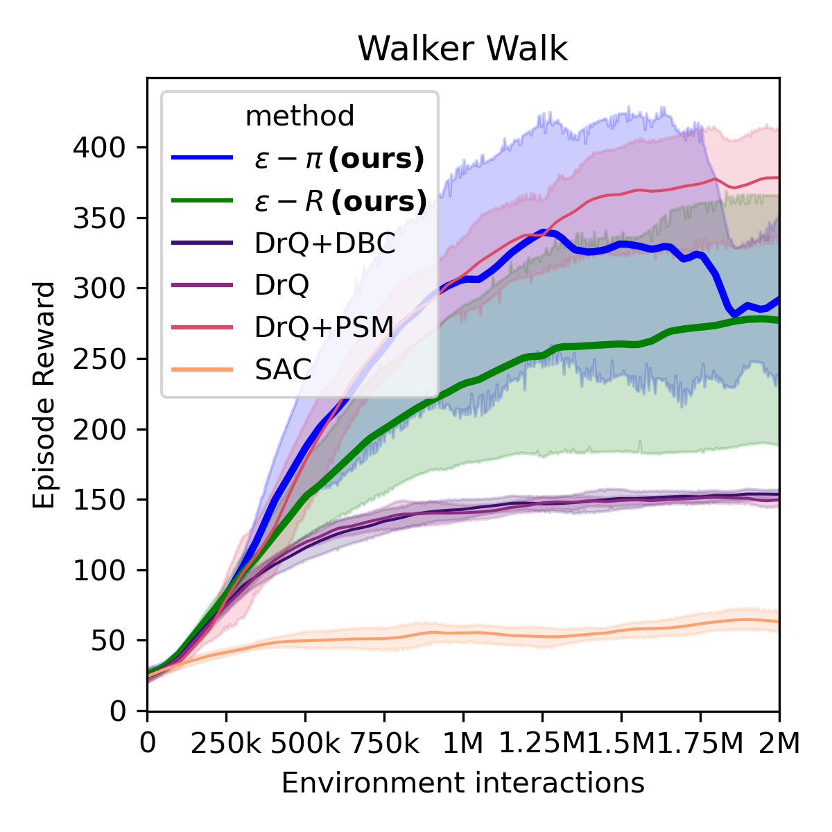
We test 666 training setups: SAC as a baseline, DrQ, which adds low-level visual augmentation, DrQ ++DBC, a reward-based bisimulation measure on top of DrQ, ϵitalic-ϵ\epsilon-R, our entagled correction for reward-based bisimulation ( G(𝒛,𝒂,𝒛,𝒂)=|R(𝒛,𝒂)R(𝒛,𝒂)|𝐺𝒛𝒂superscript𝒛superscript𝒂𝑅𝒛𝒂𝑅superscript𝒛superscript𝒂G(\bm{z},\bm{a},\bm{z}^{\prime},\bm{a}^{\prime})=|R(\bm{z},\bm{a})-R(\bm{z}^{\prime},\bm{a}^{\prime})|) on top of DrQ, DrQ++PSM, a policy-based bisimulation measure, and ϵitalic-ϵ\epsilon-π𝜋\pi, our entagled correction for policy-based bisimulation ( G(𝒛,𝒂,𝒛,𝒂)=𝔼π(𝒂|𝒛)[𝒂]𝔼π(𝒂|𝒛)[𝒂]1𝐺𝒛𝒂superscript𝒛superscript𝒂subscriptnormsubscript𝔼𝜋conditional𝒂𝒛delimited-[]𝒂subscript𝔼𝜋conditionalsuperscript𝒂superscript𝒛delimited-[]superscript𝒂1G(\bm{z},\bm{a},\bm{z}^{\prime},\bm{a}^{\prime})=||\mathbb{E}_{\pi(\bm{a}|\bm{z})}[\bm{a}]-\mathbb{E}_{\pi(\bm{a}^{\prime}|\bm{z}^{\prime})}[\bm{a}^{\prime}]||_{1}) on top of DrQ. All methods share a common architecture and hyperparameters, described in Appendix C; for bisimulation-based methods, we further tune the bisimulation strength hyperparameter β𝛽\beta, only the results for the best performing hyperparameters are shown.

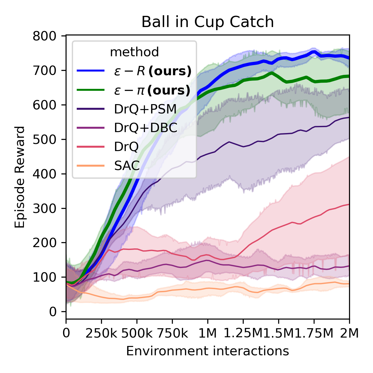
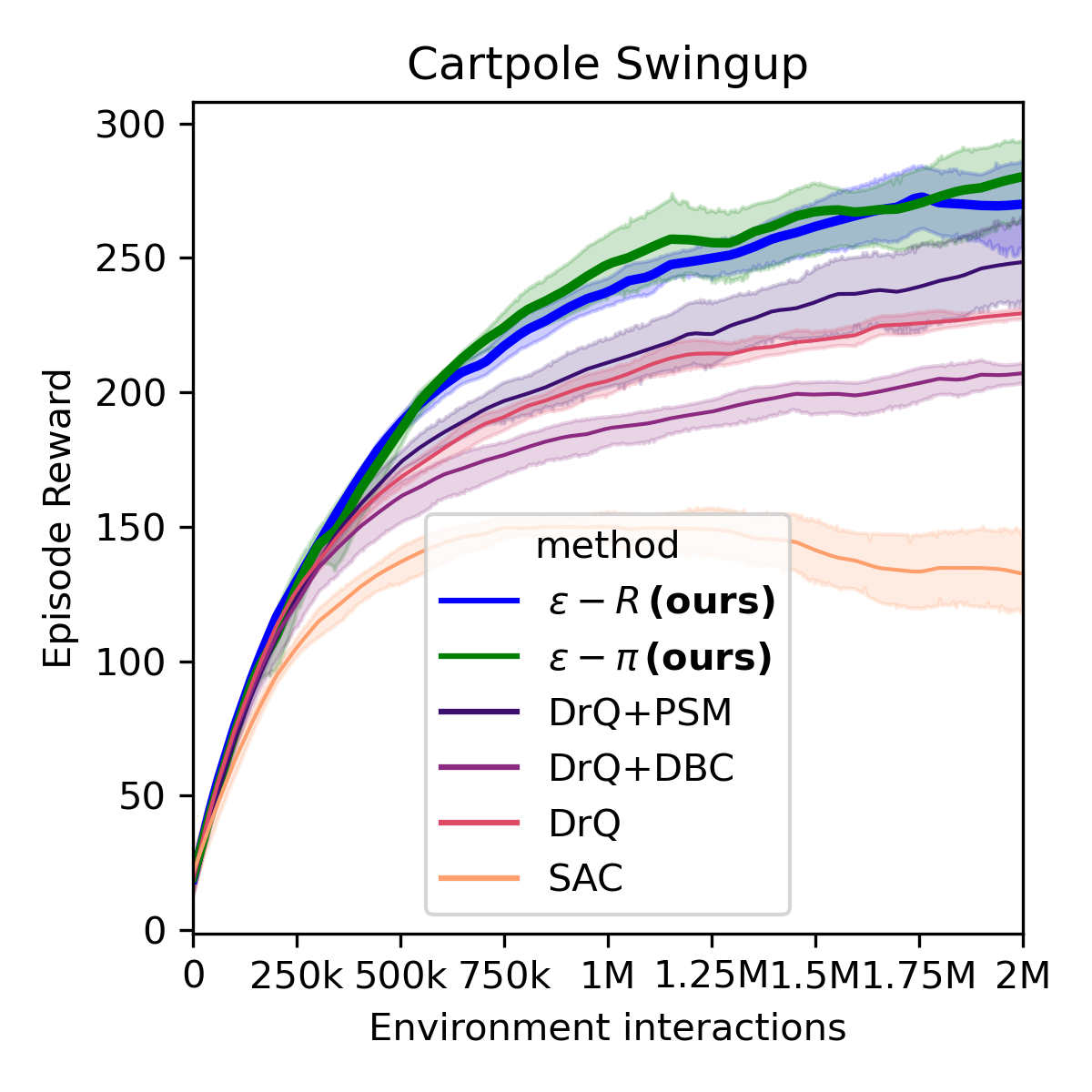
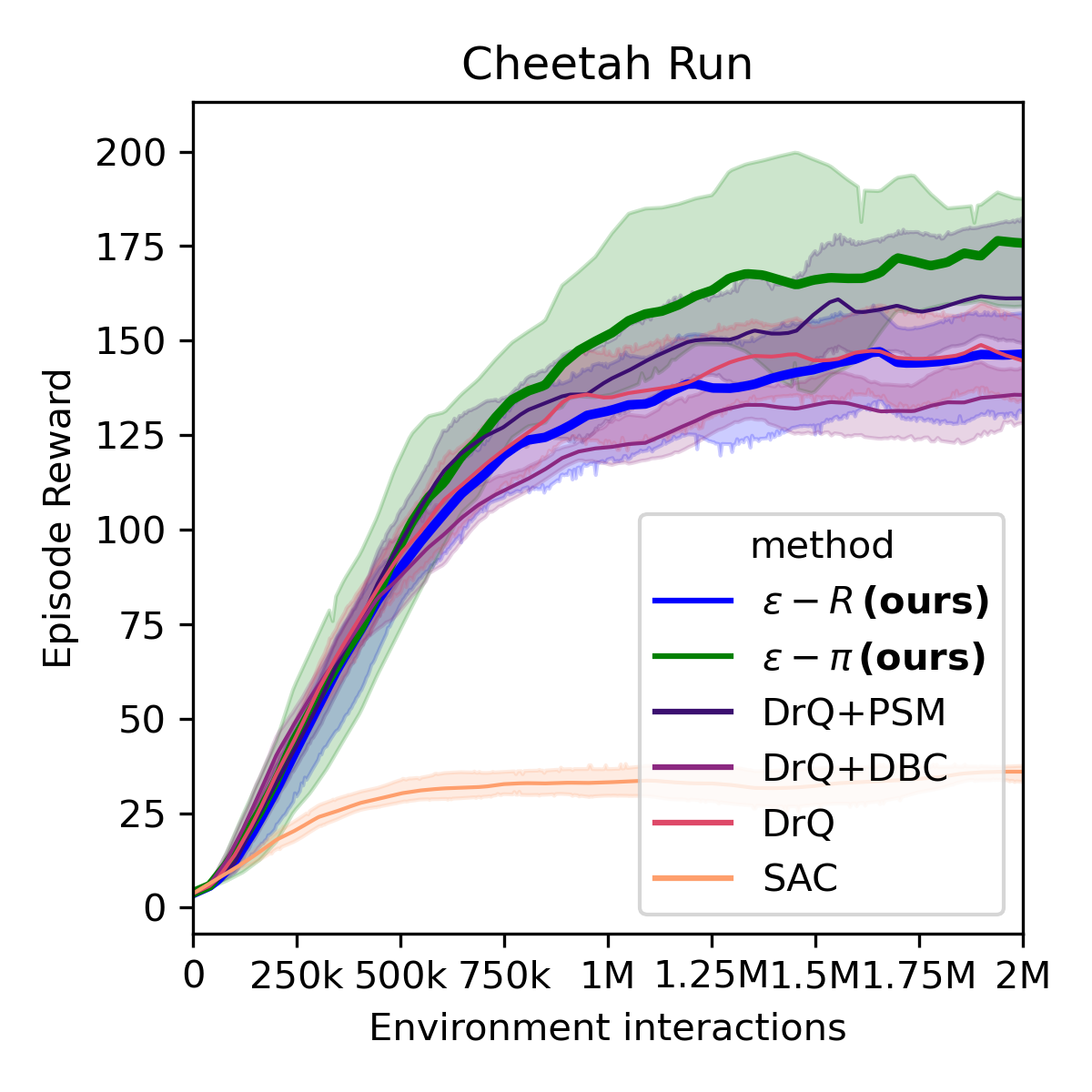
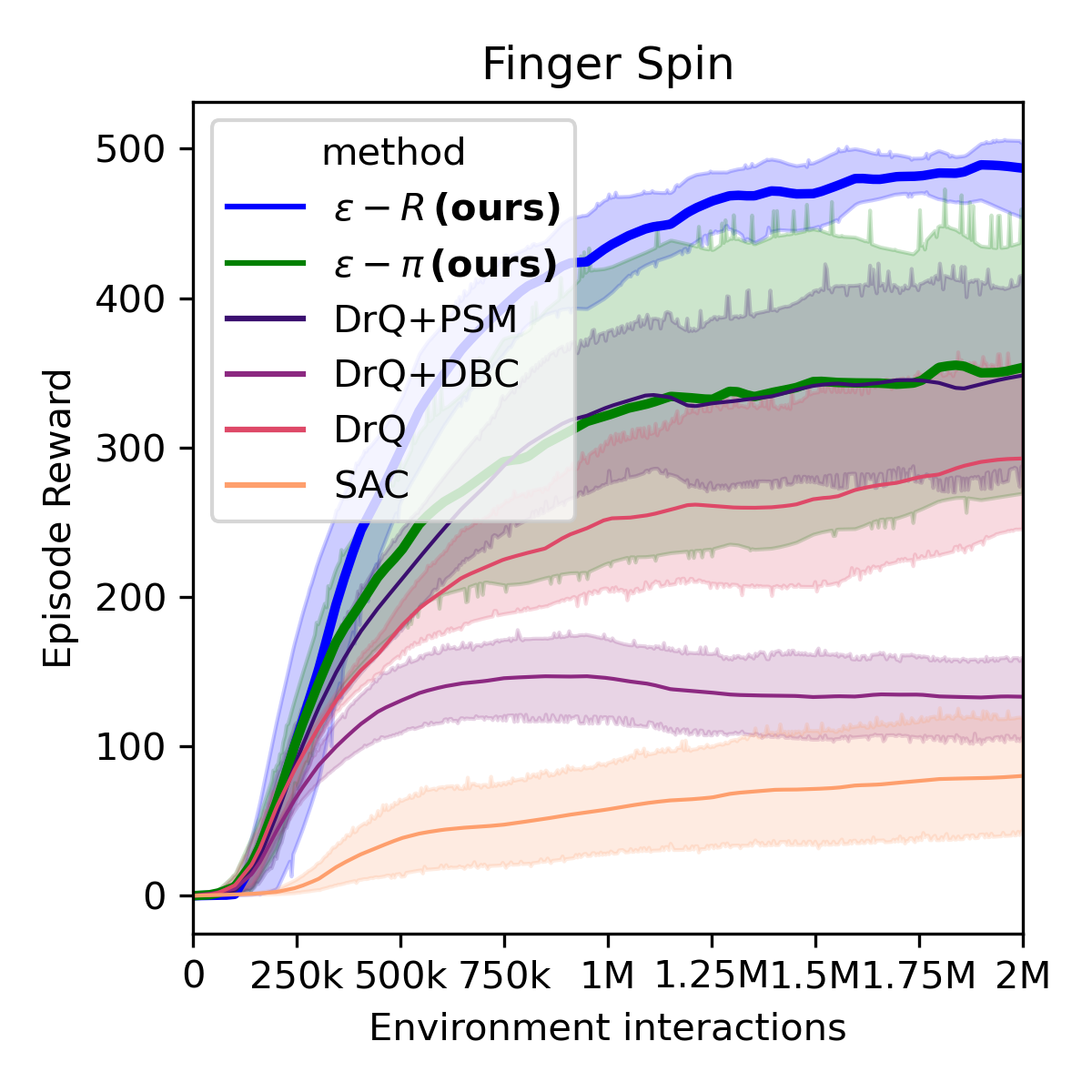
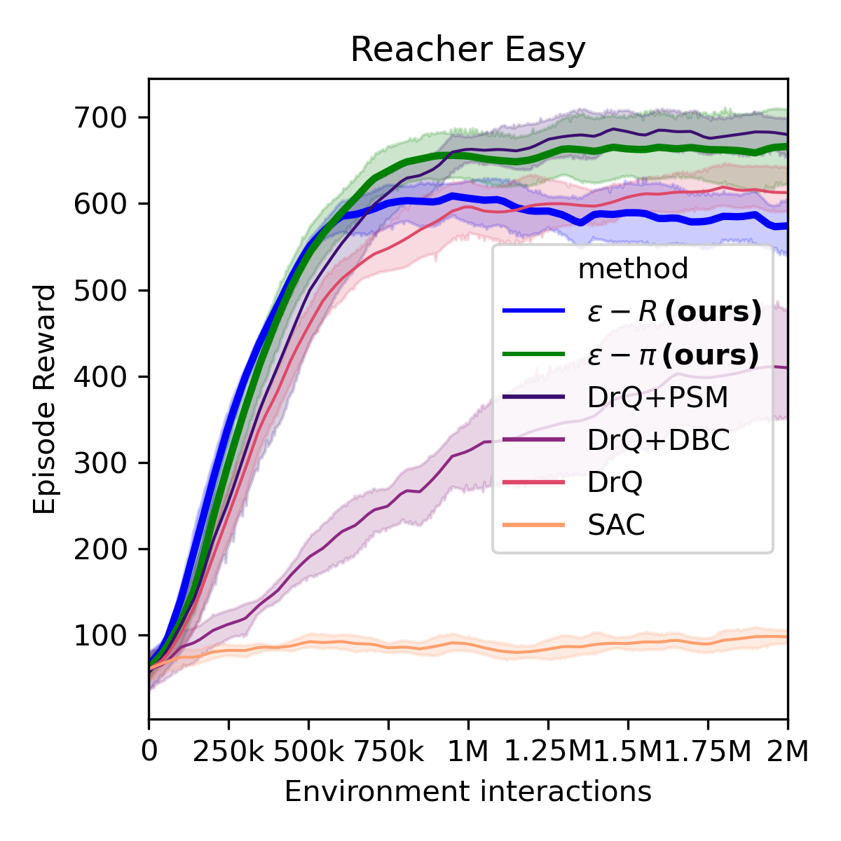
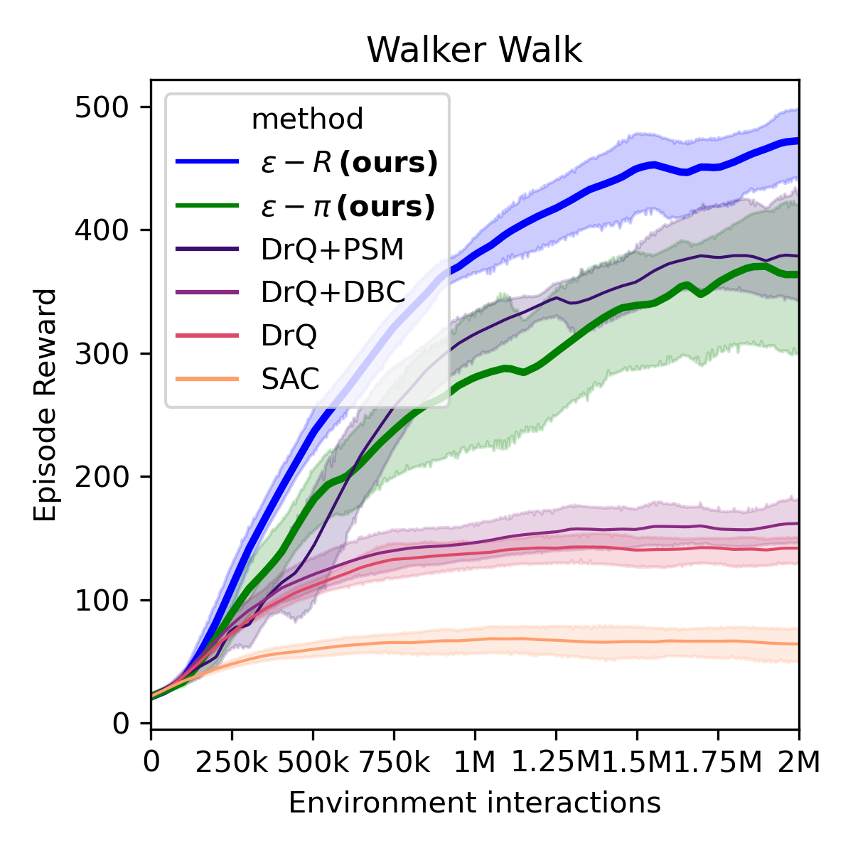
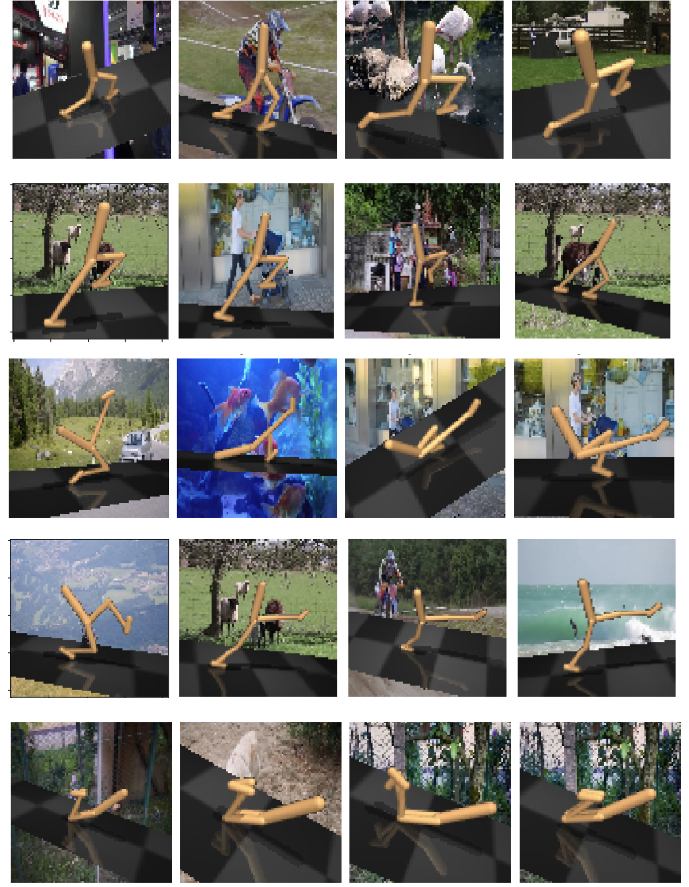
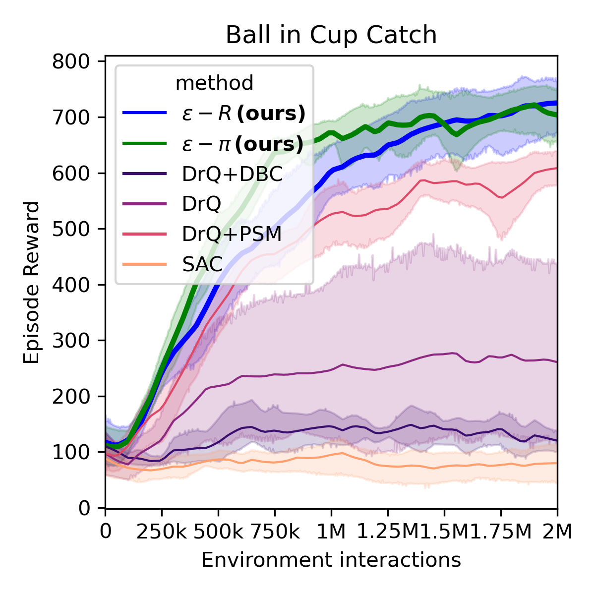
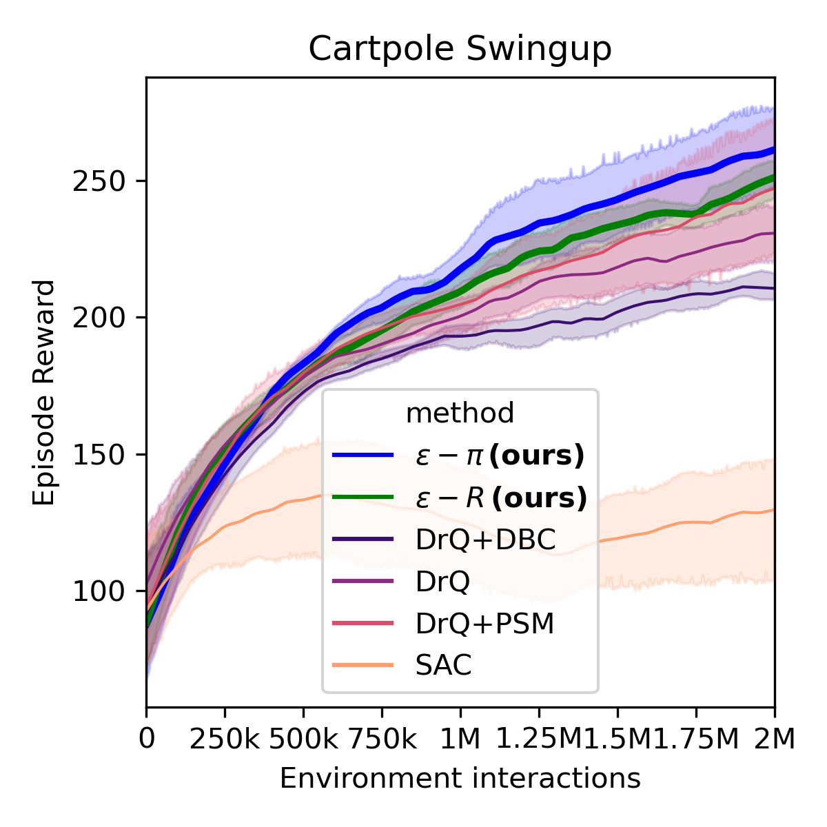
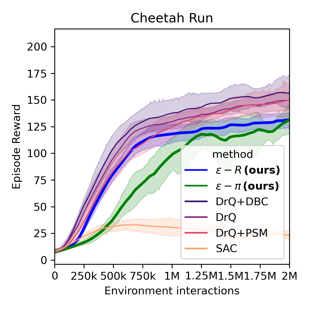
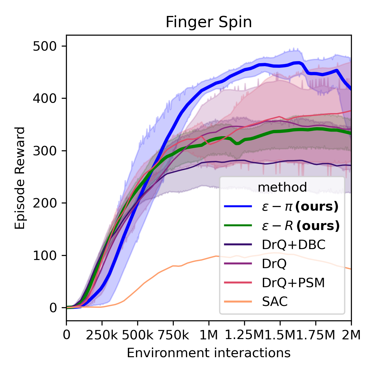
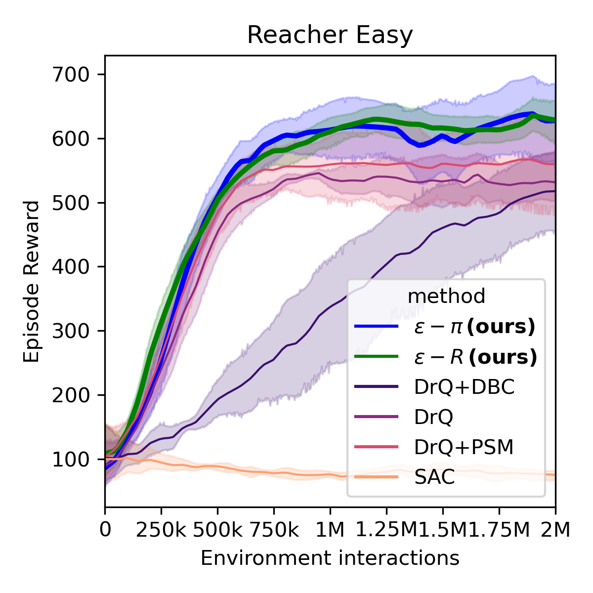
Table 1 shows the results with background distractions and camera movement, data augmentation in the form of DrQ improves on the SAC baseline, and bisimulation metrics improve on this even further, with ϵitalic-ϵ\epsilon-π𝜋\pi and ϵitalic-ϵ\epsilon-R providing the best overall results. We observe that the largest improvement provided by entanglement is seen on the DrQ+DBC to ϵitalic-ϵ\epsilon-R comparison, in some cases boosting performance over 3×3\times over the unmodified algorithm; it also alleviates failiure cases as seen in BiC, FS, and RE, where DrQ+DBC is a net loss over just the DrQ baseline. Some environments (BiC, FS, WW) show significant improvement of the bisimulation methods w.r.t. data augmentation, though none are adversely affected by the inclusion of bisimulation. The training dynamics of these methods are shown in Figure 2. Additionally, Figure 3 shows random observations, along with their closest bisimulation matches across other episodes and backgrounds on a small subset of 10 episodes acquired on the Walker Walk environment. Semantically similar situations are consistently identified regardless of background or camera position.

Table 1: Episodic reward on Distracting Control Suite with DAVIS backgrounds and hard camera distractions, 2M2𝑀2M environment steps. Mean and standard deviation computed across 5 seeds.

Method BiC CS CR FS RE WW SAC 240±9plus-or-minus2409240\pm 9 133±20plus-or-minus13320133\pm 20 36±3plus-or-minus36336\pm 3 80±51plus-or-minus805180\pm 51 98±9plus-or-minus98998\pm 9 64±17plus-or-minus641764\pm 17 DrQ 311±181plus-or-minus311181311\pm 181 229±3plus-or-minus2293229\pm 3 145±14plus-or-minus14514145\pm 14 293±72plus-or-minus29372293\pm 72 613±33plus-or-minus61333613\pm 33 142±14plus-or-minus14214142\pm 14 DrQ+DBC 132±39plus-or-minus13239132\pm 39 207±5plus-or-minus2075207\pm 5 134±12plus-or-minus13412134\pm 12 144±32plus-or-minus14432144\pm 32 410±83plus-or-minus41083410\pm 83 150±21plus-or-minus15021150\pm 21 ϵbold-italic-ϵ\bm{\epsilon}-R 𝟕𝟑𝟓±𝟑𝟕plus-or-minus73537\bm{735\pm 37} 270±22plus-or-minus27022270\pm 22 146±18plus-or-minus14618146\pm 18 𝟒𝟖𝟕±𝟑𝟑plus-or-minus48733\bm{487\pm 33} 574±42plus-or-minus57442574\pm 42 𝟒𝟕𝟐±𝟑𝟕plus-or-minus47237\bm{472\pm 37} DrQ+PSE 563±94plus-or-minus56394563\pm 94 248±20plus-or-minus24820248\pm 20 161±23plus-or-minus16123161\pm 23 348±83plus-or-minus34883348\pm 83 𝟔𝟖𝟎±𝟐𝟗plus-or-minus68029\bm{680\pm 29} 379±59plus-or-minus37959379\pm 59 ϵbold-italic-ϵ\bm{\epsilon}-π𝜋\bm{\pi} 683±103plus-or-minus683103683\pm 103 𝟐𝟖𝟎±𝟐𝟎plus-or-minus28020\bm{280\pm 20} 𝟏𝟕𝟓±𝟏𝟖plus-or-minus17518\bm{175\pm 18} 354±105plus-or-minus354105354\pm 105 666±57plus-or-minus66657666\pm 57 364±80plus-or-minus36480364\pm 80

Refer to caption
(a)
Refer to caption
(b)
Refer to caption
(c)
Refer to caption
(d)
Refer to caption
(e)
Refer to caption
(f)
Figure 2: Episodic reward on test environments in DCS benchmark with hard camera distractions and 303030 background videos. Standard deviations are collected across 555 independent seeds.
Refer to caption
(a)
Figure 3: Sample observations, alongside their closest bisimulation matches, acquired over 10 episodes on the Walker Walk environment with hard backgrounds and camera distractions. We acquired 555 independent cameras, each with its own independent motion and distracting background, to provide novel viewpoints for the bisimulation comparisons.

To test if network capacity plays a major role in these results, we repeat these experiments using a smaller architecture in Table 2. Here, all hidden layers have their size reduced from 100010001000 to 200200200 units. The results show a loss of performance across the board, suggesting that capacity is being properly utilized on the larger architecture size. Bisimulation-based methods still show the best overall performances, with reward-based bisimulation methods taking a comparatively larger hit from the reduced network capacity. The same environments that previously exhibited large performance differences between DrQ and the bisimulation-based methods continue to do so. Figure 4 shows the training dynamics in the low-capacity scenario.

Table 2: Episodic reward on Distracting Control Suite with DAVIS backgrounds and hard camera distractions, 2M2𝑀2M environment steps, low capacity network. Mean and standard deviation computed across 5 seeds.

Method BiC CS CR FS RE WW SAC 78±43plus-or-minus784378\pm 43 130±28plus-or-minus13028130\pm 28 31±7plus-or-minus31731\pm 7 74±35plus-or-minus743574\pm 35 75±10plus-or-minus751075\pm 10 63±10plus-or-minus631063\pm 10 DrQ 261±206plus-or-minus261206261\pm 206 231±13plus-or-minus23113231\pm 13 156±19plus-or-minus15619156\pm 19 341±94plus-or-minus34194341\pm 94 532±52plus-or-minus53252532\pm 52 150±6plus-or-minus1506150\pm 6 DrQ+DBC 120±21plus-or-minus12021120\pm 21 211±6plus-or-minus2116211\pm 6 162±17plus-or-minus16217162\pm 17 276±89plus-or-minus27689276\pm 89 518±80plus-or-minus51880518\pm 80 147±8plus-or-minus1478147\pm 8 ϵbold-italic-ϵ\bm{\epsilon}-R 𝟕𝟐𝟓±𝟔𝟐plus-or-minus72562\bm{725\pm 62} 251±9plus-or-minus2519251\pm 9 124±7plus-or-minus1247124\pm 7 333±37plus-or-minus33337333\pm 37 𝟔𝟐𝟖±𝟒𝟏plus-or-minus62841\bm{628\pm 41} 277±116plus-or-minus277116277\pm 116 DrQ+PSE 608±36plus-or-minus60836608\pm 36 247±33plus-or-minus24733247\pm 33 𝟏𝟕𝟏±𝟒𝟎plus-or-minus17140\bm{171\pm 40} 376±121plus-or-minus376121376\pm 121 560±90plus-or-minus56090560\pm 90 𝟑𝟕𝟖±𝟓𝟏plus-or-minus37851\bm{378\pm 51} ϵbold-italic-ϵ\bm{\epsilon}-π𝜋\bm{\pi} 704±64plus-or-minus70464704\pm 64 𝟐𝟔𝟏±𝟏𝟖plus-or-minus26118\bm{261\pm 18} 117±52plus-or-minus11752117\pm 52 𝟒𝟏𝟖±𝟗𝟕plus-or-minus41897\bm{418\pm 97} 𝟔𝟐𝟖±𝟖𝟎plus-or-minus62880\bm{628\pm 80} 292±75plus-or-minus29275292\pm 75

Refer to caption
(a)
Refer to caption
(b)
Refer to caption
(c)
Refer to caption
(d)
Refer to caption
(e)
Refer to caption
(f)
Figure 4: Episodic reward on test environments in DCS benchmark with hard camera distractions and 303030 background videos from the DAVIS dataset. Low capacity architecture. Standard deviations are collected across 555 independent seeds.
Table 3: Episodic reward on Distracting Control Suite with DAVIS backgrounds and no camera distractions, 2M2𝑀2M environment steps. Mean and standard deviation computed across 5 seeds.

Method BiC CS CR FS RE WW ϵbold-italic-ϵ\bm{\epsilon}-R 771±9plus-or-minus7719771\pm 9 𝟑𝟔𝟕±𝟐𝟗plus-or-minus36729\bm{367\pm 29} 239±48plus-or-minus23948{239\pm 48} 419±129plus-or-minus419129419\pm 129 642±35plus-or-minus64235642\pm 35 𝟓𝟒𝟏±𝟕𝟕plus-or-minus54177\bm{541\pm 77} DrQ+PSE 673±328plus-or-minus673328673\pm 328 348±51plus-or-minus34851348\pm 51 𝟑𝟎𝟓±𝟑𝟑plus-or-minus30533\bm{305\pm 33} 𝟓𝟕𝟑±𝟏𝟑𝟏plus-or-minus573131\bm{573\pm 131} 𝟕𝟎𝟑±𝟏𝟏plus-or-minus70311\bm{703\pm 11} 411±138plus-or-minus411138411\pm 138 ϵbold-italic-ϵ\bm{\epsilon}-π𝜋\bm{\pi} 𝟕𝟖𝟐±𝟖𝟒plus-or-minus78284\bm{782\pm 84} 348±51plus-or-minus34851348\pm 51 249±58plus-or-minus24958249\pm 58 528±77plus-or-minus52877528\pm 77 696±29plus-or-minus69629696\pm 29 463±103plus-or-minus463103463\pm 103

Out of the two distractions present in our benchmark, camera movement is the one least addressed by low-level augmentation techniques like the random cropping added in DrQ. For this reason, we remove camera distractions and rerun the experiments, which are shown in Table 3. Without camera distractions, all environments significantly improve their performance.

7 Discussion

This paper examines current methods for extracting task-relevant state in environments that present significant task-irrelevant distractions. We focus on bisimulation-based methods, their practical implementations, and some of the consistent estimation errors present in current methods for continuous action spaces. We propose entangled bisimulation, a new bisimulation framework that is able to eliminate estimation bias for a broad class of user-specified invariances, and is trivial to implement in many practical scenarios. We enable the use of user-specified invariances throughout the representation learning process. We empirically show how this improved estimation positively impacts performance on a variety of environments for the common reward- and policy-based invariances, and how bisimulation measures interact with standard data augmentation techniques.

Our experiments show that certain, but not all, environments are improved by the addition of bisimulation, even beyond standard data augmentation. No environments see their performance negatively affected by this addition, suggesting that this technique can be added into standard RL practice without adverse effects. We also observed that, with proper baseline architectures, reward- and policy-based bisimulation yields similar results after correcting for estimation biases.

Future work should be aimed at understanding why certain environments show large performance differences with bisimulation-based measures, while others remain unaffected. A proper understanding of what properties of an environment or a distraction are directly addressed by either data augmentation or bisimulation is needed.

References

  • Agarwal et al. (2021) Agarwal, R., Machado, M. C., Castro, P. S., and Bellemare, M. G. Contrastive behavioral similarity embeddings for generalization in reinforcement learning. arXiv preprint arXiv:2101.05265, 2021.
  • Castro (2020) Castro, P. S. Scalable methods for computing state similarity in deterministic markov decision processes. In Proceedings of the AAAI Conference on Artificial Intelligence, volume 34, pp.  10069–10076, 2020.
  • Chen et al. (2020) Chen, T., Kornblith, S., Norouzi, M., and Hinton, G. A simple framework for contrastive learning of visual representations. In International conference on machine learning, pp. 1597–1607. PMLR, 2020.
  • Chizat et al. (2020) Chizat, L., Roussillon, P., Léger, F., Vialard, F.-X., and Peyré, G. Faster wasserstein distance estimation with the sinkhorn divergence. Advances in Neural Information Processing Systems, 33, 2020.
  • Cobbe et al. (2019) Cobbe, K., Klimov, O., Hesse, C., Kim, T., and Schulman, J. Quantifying generalization in reinforcement learning. In International Conference on Machine Learning, pp. 1282–1289. PMLR, 2019.
  • Dosovitskiy et al. (2017) Dosovitskiy, A., Ros, G., Codevilla, F., Lopez, A., and Koltun, V. Carla: An open urban driving simulator. In Conference on robot learning, pp.  1–16. PMLR, 2017.
  • Duan et al. (2016) Duan, Y., Schulman, J., Chen, X., Bartlett, P. L., Sutskever, I., and Abbeel, P. Rl2: Fast reinforcement learning via slow reinforcement learning. arXiv preprint arXiv:1611.02779, 2016.
  • Espeholt et al. (2018) Espeholt, L., Soyer, H., Munos, R., Simonyan, K., Mnih, V., Ward, T., Doron, Y., Firoiu, V., Harley, T., Dunning, I., et al. Impala: Scalable distributed deep-rl with importance weighted actor-learner architectures. In International Conference on Machine Learning, pp. 1407–1416. PMLR, 2018.
  • Ferns & Precup (2014) Ferns, N. and Precup, D. Bisimulation metrics are optimal value functions. In UAI, pp.  210–219. Citeseer, 2014.
  • Ferns et al. (2004) Ferns, N., Panangaden, P., and Precup, D. Metrics for finite markov decision processes. In UAI, volume 4, pp.  162–169, 2004.
  • Ferns et al. (2011) Ferns, N., Panangaden, P., and Precup, D. Bisimulation metrics for continuous markov decision processes. SIAM Journal on Computing, 40(6):1662–1714, 2011.
  • Haarnoja et al. (2018) Haarnoja, T., Zhou, A., Abbeel, P., and Levine, S. Soft actor-critic: Off-policy maximum entropy deep reinforcement learning with a stochastic actor. In International conference on machine learning, pp. 1861–1870. PMLR, 2018.
  • Hafner et al. (2019) Hafner, D., Lillicrap, T., Ba, J., and Norouzi, M. Dream to control: Learning behaviors by latent imagination. arXiv preprint arXiv:1912.01603, 2019.
  • Henderson et al. (2018) Henderson, P., Islam, R., Bachman, P., Pineau, J., Precup, D., and Meger, D. Deep reinforcement learning that matters. In Proceedings of the AAAI conference on artificial intelligence, volume 32, 2018.
  • Hjelm et al. (2018) Hjelm, R. D., Fedorov, A., Lavoie-Marchildon, S., Grewal, K., Bachman, P., Trischler, A., and Bengio, Y. Learning deep representations by mutual information estimation and maximization. arXiv preprint arXiv:1808.06670, 2018.
  • Jaderberg et al. (2016) Jaderberg, M., Mnih, V., Czarnecki, W. M., Schaul, T., Leibo, J. Z., Silver, D., and Kavukcuoglu, K. Reinforcement learning with unsupervised auxiliary tasks. arXiv preprint arXiv:1611.05397, 2016.
  • Kaiser et al. (2019) Kaiser, L., Babaeizadeh, M., Milos, P., Osinski, B., Campbell, R. H., Czechowski, K., Erhan, D., Finn, C., Kozakowski, P., Levine, S., et al. Model-based reinforcement learning for atari. arXiv preprint arXiv:1903.00374, 2019.
  • Kalashnikov et al. (2018) Kalashnikov, D., Irpan, A., Pastor, P., Ibarz, J., Herzog, A., Jang, E., Quillen, D., Holly, E., Kalakrishnan, M., Vanhoucke, V., et al. Qt-opt: Scalable deep reinforcement learning for vision-based robotic manipulation. arXiv preprint arXiv:1806.10293, 2018.
  • Kemertas & Aumentado-Armstrong (2021) Kemertas, M. and Aumentado-Armstrong, T. Towards robust bisimulation metric learning. Advances in Neural Information Processing Systems, 34, 2021.
  • Kostrikov et al. (2020) Kostrikov, I., Yarats, D., and Fergus, R. Image augmentation is all you need: Regularizing deep reinforcement learning from pixels. arXiv preprint arXiv:2004.13649, 2020.
  • Laskin et al. (2020) Laskin, M., Lee, K., Stooke, A., Pinto, L., Abbeel, P., and Srinivas, A. Reinforcement learning with augmented data. arXiv preprint arXiv:2004.14990, 2020.
  • Lillicrap et al. (2015) Lillicrap, T. P., Hunt, J. J., Pritzel, A., Heess, N., Erez, T., Tassa, Y., Silver, D., and Wierstra, D. Continuous control with deep reinforcement learning. arXiv preprint arXiv:1509.02971, 2015.
  • Pont-Tuset et al. (2017) Pont-Tuset, J., Perazzi, F., Caelles, S., Arbeláez, P., Sorkine-Hornung, A., and Van Gool, L. The 2017 davis challenge on video object segmentation. arXiv preprint arXiv:1704.00675, 2017.
  • Sekar et al. (2020) Sekar, R., Rybkin, O., Daniilidis, K., Abbeel, P., Hafner, D., and Pathak, D. Planning to explore via self-supervised world models. In International Conference on Machine Learning, pp. 8583–8592. PMLR, 2020.
  • Song et al. (2019) Song, X., Jiang, Y., Tu, S., Du, Y., and Neyshabur, B. Observational overfitting in reinforcement learning. arXiv preprint arXiv:1912.02975, 2019.
  • Srinivas et al. (2020) Srinivas, A., Laskin, M., and Abbeel, P. Curl: Contrastive unsupervised representations for reinforcement learning. arXiv preprint arXiv:2004.04136, 2020.
  • Stone et al. (2021) Stone, A., Ramirez, O., Konolige, K., and Jonschkowski, R. The distracting control suite–a challenging benchmark for reinforcement learning from pixels. arXiv preprint arXiv:2101.02722, 2021.
  • Tachet et al. (2018) Tachet, R., Bachman, P., and van Seijen, H. Learning invariances for policy generalization. arXiv preprint arXiv:1809.02591, 2018.
  • Zhang et al. (2020) Zhang, A., McAllister, R., Calandra, R., Gal, Y., and Levine, S. Learning invariant representations for reinforcement learning without reconstruction. arXiv preprint arXiv:2006.10742, 2020.

Appendix A Theorem Proofs

Here we provide the proof for all theorems stated in this work.

Theorem 4.6.

Define the metric operator ϵ:𝕄𝕄:superscriptitalic-ϵ𝕄𝕄\mathcal{F}^{\epsilon}:\mathbb{M}\rightarrow\mathbb{M} as

ϵ(d)(𝒛,𝒛)=𝔼𝒂,𝒂γϵ(π(|𝒛),π(|𝒛))[G(𝒛,𝒂,𝒛,𝒂)+c𝒲1(P(𝒛+|𝒛,π),P(𝒛+|𝒛,π);d)].\mathcal{F}_{\epsilon}(d)(\bm{z},\bm{z^{\prime}})=\mathbb{E}_{\bm{a},\bm{a}^{\prime}\sim\gamma^{\epsilon}(\pi(\cdot|\bm{z}),\pi(\cdot|\bm{z}^{\prime}))}[G(\bm{z},\bm{a},\bm{z}^{\prime},\bm{a}^{\prime})+c\mathcal{W}_{1}(P(\bm{z}_{+}|\bm{z},\pi),P(\bm{z}^{\prime}_{+}|\bm{z}^{\prime},\pi);d)]. (22)

Then, with c[0,1)𝑐01c\in[0,1), ϵsubscriptitalic-ϵ\mathcal{F}_{\epsilon} has at least a fixed point dϵsubscript𝑑italic-ϵd_{\epsilon} which is a bisimulation metric.

Proof.

We first observe that, since G is non-negative

A{(𝒛,𝒛):𝔼𝒂,𝒂γϵ(π(|𝒛),π(|𝒛))G(𝒛,𝒂,𝒛,𝒂)=0},B{(𝒛,𝒛):G(𝒛,𝒂,𝒛,𝒂)=0,𝒂,𝒂Supp(γϵ(π(|𝒛),π(|𝒛)))(𝒛,𝒛)A(𝒛,𝒛)B,\begin{array}[]{l}A\coloneqq\{(\bm{z},\bm{z^{\prime}}):\mathbb{E}_{\bm{a},\bm{a}^{\prime}\sim\gamma^{\epsilon}(\pi(\cdot|\bm{z}),\pi(\cdot|\bm{z}^{\prime}))}G(\bm{z},\bm{a},\bm{z}^{\prime},\bm{a}^{\prime})=0\},\\ B\coloneqq\{(\bm{z},\bm{z^{\prime}}):G(\bm{z},\bm{a},\bm{z}^{\prime},\bm{a}^{\prime})=0,\forall\bm{a},\bm{a}^{\prime}\in\textit{Supp}(\gamma^{\epsilon}(\pi(\cdot|\bm{z}),\pi(\cdot|\bm{z}^{\prime})))\\ (\bm{z},\bm{z^{\prime}})\in A\iff(\bm{z},\bm{z^{\prime}})\in B,\end{array} (23)

except on a zero-measure set in γϵ(π(|𝒛),π(|𝒛))\gamma^{\epsilon}(\pi(\cdot|\bm{z}),\pi(\cdot|\bm{z}^{\prime})).

The rest of the proof largely mimics the proof of Theorem 4.5 in (Ferns et al., 2004), and its adaptation in Theorem 2 in (Castro, 2020), which is Theorem 1 in this paper, we largely use the same notation when appropriate, and refer the reader to (Ferns et al., 2004) for the details ommited in this proof. Lemma 4.1 in (Ferns et al., 2004) holds for definition 4.4. We make use of the same distance ordering on 𝕄𝕄\mathbb{M} where ddd(𝒛,𝒛)d(𝒛,𝒛),𝒛,𝒛𝒵2iff𝑑superscript𝑑formulae-sequence𝑑𝒛superscript𝒛bold-′superscript𝑑𝒛superscript𝒛bold-′for-all𝒛superscript𝒛bold-′superscript𝒵2d\leq d^{\prime}\iff d(\bm{z},\bm{z^{\prime}})\leq d^{\prime}(\bm{z},\bm{z^{\prime}}),\,\forall\bm{z},\bm{z^{\prime}}\in\mathcal{Z}^{2}, this produces an ω𝜔\omega-cpo (an ω𝜔\omega complete partial order) with bottom perpendicular-to\perp the everywhere zero distance. Since we also use 𝒲1subscript𝒲1\mathcal{W}_{1} to measure state distribution distances in ϵsuperscriptitalic-ϵ\mathcal{F}^{\epsilon}, then Lemma 4.4 in (Ferns et al., 2004) also applies (continuity of 𝒲1subscript𝒲1\mathcal{W}_{1}).

The remaining piece for the proof is showing that ϵsuperscriptitalic-ϵ\mathcal{F}^{\epsilon} is continuous, meaning that for every ω𝜔\omega-chain {dn}subscript𝑑𝑛\{d_{n}\} (an increasing sequence of metrics), then ϵ(n{dn})=n{ϵ(dn)}superscriptitalic-ϵsubscript𝑛subscript𝑑𝑛subscript𝑛superscriptitalic-ϵsubscript𝑑𝑛\mathcal{F}^{\epsilon}(\cup_{n}\{d_{n}\})=\cup_{n}\{\mathcal{F}^{\epsilon}(d_{n})\}, where n{dn}(𝒛,𝒛)=supndn(𝒛,𝒛)subscript𝑛subscript𝑑𝑛𝒛superscript𝒛bold-′subscriptsupremum𝑛subscript𝑑𝑛𝒛superscript𝒛bold-′\cup_{n}\{d_{n}\}(\bm{z},\bm{z^{\prime}})=\sup_{n\in\mathbb{N}}d_{n}(\bm{z},\bm{z^{\prime}}). This follows from

ϵ(n{dn})=𝔼𝒂,𝒂γϵ(π(|𝒛),π(|𝒛))[G(𝒛,𝒂,𝒛,𝒂)+c𝒲1(P(𝒛+|𝒛,𝒂),P(𝒛+|𝒛,𝒂);n{dn})],=supn{𝔼𝒂,𝒂γϵ(π(|𝒛),π(|𝒛))[G(𝒛,𝒂,𝒛,𝒂)+c𝒲1(P(𝒛+|𝒛,𝒂),P(𝒛+|𝒛,𝒂);dn)]},=supnϵ(dn),\begin{array}[]{rl}\mathcal{F}^{\epsilon}(\cup_{n}\{d_{n}\})&=\mathbb{E}_{\bm{a},\bm{a}^{\prime}\sim\gamma^{\epsilon}(\pi(\cdot|\bm{z}),\pi(\cdot|\bm{z}^{\prime}))}[G(\bm{z},\bm{a},\bm{z}^{\prime},\bm{a}^{\prime})\\ &+c\mathcal{W}_{1}(P(\bm{z}_{+}|\bm{z},\bm{a}),P(\bm{z}^{\prime}_{+}|\bm{z}^{\prime},\bm{a}^{\prime});\cup_{n}\{d_{n}\})],\\ &=\sup_{n\in\mathbb{N}}\big{\{}\mathbb{E}_{\bm{a},\bm{a}^{\prime}\sim\gamma^{\epsilon}(\pi(\cdot|\bm{z}),\pi(\cdot|\bm{z}^{\prime}))}[G(\bm{z},\bm{a},\bm{z}^{\prime},\bm{a}^{\prime})\\ &+c\mathcal{W}_{1}(P(\bm{z}_{+}|\bm{z},\bm{a}),P(\bm{z}^{\prime}_{+}|\bm{z}^{\prime},\bm{a}^{\prime});d_{n})]\big{\}},\\ &=\sup_{n\in\mathbb{N}}\mathcal{F}^{\epsilon}(d_{n}),\\ \end{array} (24)

Where the second equality follows by the continuity of 𝒲1subscript𝒲1\mathcal{W}_{1} w.r.t. the metric dnsubscript𝑑𝑛d_{n}. The rest of the proof follows (Ferns et al., 2004).

Lemma 4.7.

Let Eπsuperscript𝐸𝜋E^{\pi} be the largest π𝜋\pi-bisimulation relation, and let EPSMsuperscript𝐸𝑃𝑆𝑀E^{PSM} likewise be the largest average-action bisimulation relation in (Agarwal et al., 2021). The entangled bisimulation relation Eϵsuperscript𝐸italic-ϵE^{\epsilon} satisfies

EϵEπEϵEPSMsuperscript𝐸italic-ϵabsentsuperscript𝐸𝜋superscript𝐸italic-ϵabsentsuperscript𝐸𝑃𝑆𝑀\begin{array}[]{rl}E^{\epsilon}&\subseteq E^{\pi}\\ E^{\epsilon}&\subseteq E^{PSM}\\ \end{array} (25)

for the choice of state-action similarity metrics G(𝒛,𝒂,𝒛,𝒂)=R(𝒛,𝒂)R(𝒛,𝒂)1𝐺𝒛𝒂superscript𝒛superscript𝒂subscriptnorm𝑅𝒛𝒂𝑅superscript𝒛superscript𝒂1G(\bm{z},\bm{a},\bm{z}^{\prime},\bm{a}^{\prime})=||R(\bm{z},\bm{a})-R(\bm{z}^{\prime},\bm{a}^{\prime})||_{1} and G(𝒛,𝒂,𝒛,𝒂)=𝔼π(𝒂|𝒛)[𝒂]𝔼π(𝒂|𝒛)[𝒂]1𝐺𝒛𝒂superscript𝒛superscript𝒂subscriptnormsubscript𝔼𝜋conditional𝒂𝒛delimited-[]𝒂subscript𝔼𝜋conditionalsuperscript𝒂superscript𝒛delimited-[]superscript𝒂1G(\bm{z},\bm{a},\bm{z}^{\prime},\bm{a}^{\prime})=||\mathbb{E}_{\pi(\bm{a}|\bm{z})}[\bm{a}]-\mathbb{E}_{\pi(\bm{a}^{\prime}|\bm{z}^{\prime})}[\bm{a}^{\prime}]||_{1} respectively

Proof.

The proof is identical in both cases, so we focus on the reward-based case with G(𝒛,𝒂,𝒛,𝒂)=R(𝒛,𝒂)R(𝒛,𝒂)1𝐺𝒛𝒂superscript𝒛superscript𝒂subscriptnorm𝑅𝒛𝒂𝑅superscript𝒛superscript𝒂1G(\bm{z},\bm{a},\bm{z}^{\prime},\bm{a}^{\prime})=||R(\bm{z},\bm{a})-R(\bm{z}^{\prime},\bm{a}^{\prime})||_{1}. From Jensen’s inequality we have

𝔼𝒂,𝒂γϵ(π(|𝒛),π(|𝒛))[G(𝒛,𝒂,𝒛,𝒂)]𝔼𝒂π(|𝒛)R(𝒛,𝒂)𝔼𝒂π(|𝒛)R(𝒛,𝒂)1=R(𝒛,π)R(𝒛,π)1.\begin{array}[]{rl}\mathbb{E}_{{\bm{a},\bm{a^{\prime}}\sim\gamma^{\epsilon}(\pi(\cdot|\bm{z}),\pi(\cdot|\bm{z}^{\prime}))}}[G(\bm{z},\bm{a},\bm{z}^{\prime},\bm{a}^{\prime})]&\geq||\mathbb{E}_{\bm{a}\sim\pi(\cdot|\bm{z})}R(\bm{z},\bm{a})-\mathbb{E}_{\bm{a}^{\prime}\sim\pi(\cdot|\bm{z}^{\prime})}R(\bm{z}^{\prime},\bm{a}^{\prime})||_{1}\\ &=||R(\bm{z},\pi)-R(\bm{z}^{\prime},\pi)||_{1}.\\ \end{array} (26)

And, likewise, for any metric d𝑑d we have

𝔼𝒂,𝒂γϵ(π(|𝒛),π(|𝒛))𝒲1(P(𝒛+|𝒛,𝒂),P(𝒛+|𝒛,𝒂);d)𝒲1(P(𝒛+|𝒛,π),P(𝒛+|𝒛,π);d)\begin{array}[]{rl}\mathbb{E}_{{\bm{a},\bm{a^{\prime}}\sim\gamma^{\epsilon}(\pi(\cdot|\bm{z}),\pi(\cdot|\bm{z}^{\prime}))}}\mathcal{W}_{1}(P(\bm{z}_{+}|\bm{z},\bm{a}),P(\bm{z}^{\prime}_{+}|\bm{z}^{\prime},\bm{a}^{\prime});d)&\geq\mathcal{W}_{1}(P(\bm{z}_{+}|\bm{z},\pi),P(\bm{z}^{\prime}_{+}|\bm{z}^{\prime},\pi);d)\end{array} (27)

Then, we observe that ϵ(d)π(d)superscriptitalic-ϵ𝑑superscript𝜋𝑑\mathcal{F}^{\epsilon}(d)\geq\mathcal{F}^{\pi}(d), and therefore dϵdπsuperscript𝑑italic-ϵsuperscript𝑑𝜋d^{\epsilon}\geq d^{\pi}. From this we conclude that any state pair (𝒛,𝒛)Eϵ𝒛superscript𝒛bold-′superscript𝐸italic-ϵ(\bm{z},\bm{z^{\prime}})\in E^{\epsilon} satisfies 0dπ(𝒛,𝒛)dϵ(𝒛,𝒛)=00superscript𝑑𝜋𝒛superscript𝒛bold-′superscript𝑑italic-ϵ𝒛superscript𝒛bold-′00\leq d^{\pi}(\bm{z},\bm{z^{\prime}})\leq d^{\epsilon}(\bm{z},\bm{z^{\prime}})=0 and therefore (𝒛,𝒛)Eπ𝒛superscript𝒛bold-′superscript𝐸𝜋(\bm{z},\bm{z^{\prime}})\in E^{\pi}.

Theorem 4.8.

Given an MDP \mathcal{M}, policy π𝜋\pi, and a state-action similarity metric G𝐺G. Define the metric operator ϵ¯:𝕄𝕄:subscript¯italic-ϵ𝕄𝕄\mathcal{F}_{\bar{\epsilon}}:\mathbb{M}\rightarrow\mathbb{M} as

ϵ¯(d)(𝒛,𝒛)=𝔼(𝒂,𝒂)γϵ(π(|𝒛),π(|𝒛))(𝒛+,𝒛+)γϵ(P(|𝒛,𝒂),P(|𝒛,𝒂))[G(𝒛,𝒂,𝒛,𝒂)+cdϕ(𝒛+,𝒛+)].\mathcal{F}_{\bar{\epsilon}}(d)(\bm{z},\bm{z^{\prime}})=\mathbb{E}_{\begin{subarray}{c}(\bm{a},\bm{a^{\prime}})\sim\gamma^{\epsilon}(\pi(\cdot|\bm{z}),\pi(\cdot|\bm{z}^{\prime}))\\ (\bm{z}_{+},\bm{z}^{\prime}_{+})\sim\gamma^{\epsilon}(P(\cdot|\bm{z},\bm{a}),P(\cdot|\bm{z}^{\prime},\bm{a}^{\prime}))\end{subarray}}[G(\bm{z},\bm{a},\bm{z}^{\prime},\bm{a}^{\prime})+cd_{\phi}(\bm{z}_{+},\bm{z}^{\prime}_{+})]. (28)

Then, ϵ¯subscript¯italic-ϵ\mathcal{F}_{\bar{\epsilon}} has at least a fixed point dϵ¯subscript𝑑¯italic-ϵd_{\bar{\epsilon}} satisfying dϵ¯dϵsubscript𝑑¯italic-ϵsubscript𝑑italic-ϵd_{\bar{\epsilon}}\geq d_{\epsilon}, and (𝒛,𝒛)Eϵdϵ¯(𝒛,𝒛)=0𝒛superscript𝒛bold-′superscript𝐸italic-ϵsubscript𝑑¯italic-ϵ𝒛superscript𝒛bold-′0(\bm{z},\bm{z^{\prime}})\in E^{\epsilon}\rightarrow d_{\bar{\epsilon}}(\bm{z},\bm{z^{\prime}})=0, in particular, dϵ¯(𝒛,𝒛)=0,𝒛𝒵formulae-sequencesubscript𝑑¯italic-ϵ𝒛𝒛0for-all𝒛𝒵d_{\bar{\epsilon}}(\bm{z},\bm{z})=0,\,\forall\bm{z}\in\mathcal{Z}.

Further, if the state transition function is coordinate independent (P(𝒛+𝒛,𝒂)=ΠiPi(zi,+𝒛,𝒂)𝒛+,𝒛,𝒂𝑃conditionalsubscript𝒛𝒛𝒂subscriptΠ𝑖subscript𝑃𝑖conditionalsubscript𝑧𝑖𝒛𝒂for-allsubscript𝒛𝒛𝒂P(\bm{z}_{+}\mid\bm{z},\bm{a})=\Pi_{i}P_{i}(z_{i,+}\mid\bm{z},\bm{a})\,\forall\bm{z}_{+},\bm{z},\bm{a}), and dϵ¯subscript𝑑¯italic-ϵd_{\bar{\epsilon}} is of the form

dϵ¯(𝒛,𝒛)=i=[n]j=[p]wi,j|zizi|j,wi,j0i,j,p>0,formulae-sequencesubscript𝑑¯italic-ϵ𝒛superscript𝒛subscript𝑖delimited-[]𝑛𝑗delimited-[]𝑝subscript𝑤𝑖𝑗superscriptsubscript𝑧𝑖subscriptsuperscript𝑧𝑖𝑗formulae-sequencesubscript𝑤𝑖𝑗0for-all𝑖𝑗𝑝0d_{\bar{\epsilon}}(\bm{z},\bm{z}^{\prime})=\sum\limits_{\begin{subarray}{c}i=[n]\\ j=[p]\end{subarray}}w_{i,j}|z_{i}-z^{\prime}_{i}|^{j},\;w_{i,j}\geq 0\forall i,j,\;p>0, (29)

then the bound is tight, that is

dϵ(𝒛,𝒛)=dϵ¯(𝒛,𝒛)=𝔼(𝒂,𝒂)γϵ(π(|𝒛),π(|𝒛))(𝒛+,𝒛+)γϵ(P(|𝒛,𝒂),P(|𝒛,𝒂))[G(𝒛,𝒂,𝒛,𝒂)+cdϵ(𝒛+,𝒛+)].\begin{array}[]{rl}d_{\epsilon}(\bm{z},\bm{z}^{\prime})&=d_{\bar{\epsilon}}(\bm{z},\bm{z}^{\prime})\\ &=\mathbb{E}_{\begin{subarray}{c}(\bm{a},\bm{a^{\prime}})\sim\gamma^{\epsilon}(\pi(\cdot|\bm{z}),\pi(\cdot|\bm{z}^{\prime}))\\ (\bm{z}_{+},\bm{z}^{\prime}_{+})\sim\gamma^{\epsilon}(P(\cdot|\bm{z},\bm{a}),P(\cdot|\bm{z}^{\prime},\bm{a}^{\prime}))\end{subarray}}[G(\bm{z},\bm{a},\bm{z}^{\prime},\bm{a}^{\prime})+cd_{\epsilon}(\bm{z}_{+},\bm{z}^{\prime}_{+})].\end{array} (30)

Proof.

The proof will be split in three parts, we first prove that dϵ¯subscript𝑑¯italic-ϵd_{\bar{\epsilon}} exists and is an upper bound for dϵsubscript𝑑italic-ϵd_{\epsilon} on every state pair, we then prove that dϵ¯subscript𝑑¯italic-ϵd_{\bar{\epsilon}} is zero on ϵitalic-ϵ\epsilon-bisimilar states, and, lastly, we prove that the bound is tight for coordinate-independent transition functions if the distance function satisfies the prescribed functional form. To reduce notation clutter throughout the proof, we drop the state and action conditionals by noting P(𝒛+)P(|𝒛,𝒂)P(\bm{z}_{+})\coloneqq P(\cdot|\bm{z},\bm{a}), and, likewise, Q(𝒛+)P(|𝒛,𝒂)Q(\bm{z}_{+}^{\prime})\coloneqq P(\cdot|\bm{z}^{\prime},\bm{a}^{\prime}). Additionally, we denote γPϵγϵ(P(|𝒛,𝒂),P(|𝒛,𝒂))\gamma^{\epsilon}_{P}\coloneqq\gamma^{\epsilon}(P(\cdot|\bm{z},\bm{a}),P(\cdot|\bm{z},\bm{a}^{\prime})) and γπϵγϵ(π(𝒛),π(𝒛))\gamma^{\epsilon}_{\pi}\coloneqq\gamma^{\epsilon}(\pi(\cdot\mid\bm{z}),\pi(\cdot\mid\bm{z}^{\prime})).

Upper bound:

To prove the existence of the fixed point metric dϵ¯subscript𝑑¯italic-ϵd_{\bar{\epsilon}}, we again mimic the proof of Theorem 4.5 in (Ferns et al., 2004), only now we need to prove that the operation T(d)𝔼(𝒂,𝒂)γπϵ(𝒛+,𝒛+)γPϵ[d(𝒛+,𝒛+)]𝑇𝑑subscript𝔼similar-to𝒂superscript𝒂bold-′subscriptsuperscript𝛾italic-ϵ𝜋similar-tosubscript𝒛subscriptsuperscript𝒛subscriptsuperscript𝛾italic-ϵ𝑃delimited-[]𝑑subscript𝒛subscriptsuperscript𝒛T(d)\coloneqq\mathbb{E}_{\begin{subarray}{c}(\bm{a},\bm{a^{\prime}})\sim\gamma^{\epsilon}_{\pi}\\ (\bm{z}_{+},\bm{z}^{\prime}_{+})\sim\gamma^{\epsilon}_{P}\end{subarray}}[d(\bm{z}_{+},\bm{z}^{\prime}_{+})] is continuous (the analog of Lemma 4.4 in that work).

This amounts to observing that, on an ω𝜔\omega-chain777Recall that an ω𝜔\omega-chain satisfies didjsubscript𝑑𝑖subscript𝑑𝑗d_{i}\leq d_{j} for every j>i𝑗𝑖j>i, and also n{dn}(𝒛,𝒛)=supndn(𝒛,𝒛)subscript𝑛subscript𝑑𝑛𝒛superscript𝒛bold-′subscriptsupremum𝑛subscript𝑑𝑛𝒛superscript𝒛bold-′\cup_{n}\{d_{n}\}(\bm{z},\bm{z^{\prime}})=\sup_{n\in\mathbb{N}}d_{n}(\bm{z},\bm{z^{\prime}}), we also define didjdi(𝒛,𝒛)dj(𝒛,𝒛)(𝒛,𝒛)𝒵2iffsubscript𝑑𝑖subscript𝑑𝑗subscript𝑑𝑖𝒛superscript𝒛bold-′subscript𝑑𝑗𝒛superscript𝒛bold-′for-all𝒛superscript𝒛bold-′superscript𝒵2d_{i}\leq d_{j}\iff d_{i}(\bm{z},\bm{z^{\prime}})\leq d_{j}(\bm{z},\bm{z^{\prime}})\,\forall\,(\bm{z},\bm{z^{\prime}})\in\mathcal{Z}^{2} {dn}subscript𝑑𝑛\{d_{n}\},

T(n{dn})=𝔼(𝒂,𝒂)γπϵ(𝒛+,𝒛+)γPϵ[n{dn}(𝒛+,𝒛+)],=supn𝔼(𝒂,𝒂)γπϵ(𝒛+,𝒛+)γPϵ[dn(𝒛+,𝒛+)]=supnT(dn).𝑇subscript𝑛subscript𝑑𝑛absentsubscript𝔼similar-to𝒂superscript𝒂bold-′subscriptsuperscript𝛾italic-ϵ𝜋similar-tosubscript𝒛subscriptsuperscript𝒛subscriptsuperscript𝛾italic-ϵ𝑃delimited-[]subscript𝑛subscript𝑑𝑛subscript𝒛subscriptsuperscript𝒛missing-subexpressionabsentsubscriptsupremum𝑛subscript𝔼similar-to𝒂superscript𝒂bold-′subscriptsuperscript𝛾italic-ϵ𝜋similar-tosubscript𝒛subscriptsuperscript𝒛subscriptsuperscript𝛾italic-ϵ𝑃delimited-[]subscript𝑑𝑛subscript𝒛subscriptsuperscript𝒛missing-subexpressionabsentsubscriptsupremum𝑛𝑇subscript𝑑𝑛\begin{array}[]{rl}T(\cup_{n}\{d_{n}\})&=\mathbb{E}_{\begin{subarray}{c}(\bm{a},\bm{a^{\prime}})\sim\gamma^{\epsilon}_{\pi}\\ (\bm{z}_{+},\bm{z}^{\prime}_{+})\sim\gamma^{\epsilon}_{P}\end{subarray}}[\cup_{n}\{d_{n}\}(\bm{z}_{+},\bm{z}^{\prime}_{+})],\\ &=\sup_{n\in\mathbb{N}}\mathbb{E}_{\begin{subarray}{c}(\bm{a},\bm{a^{\prime}})\sim\gamma^{\epsilon}_{\pi}\\ (\bm{z}_{+},\bm{z}^{\prime}_{+})\sim\gamma^{\epsilon}_{P}\end{subarray}}[d_{n}(\bm{z}_{+},\bm{z}^{\prime}_{+})]\\ &=\sup_{n\in\mathbb{N}}T(d_{n}).\\ \end{array} (31)

The rest of the proof of existence of a fixed point needs to show continuity of ϵ¯subscript¯italic-ϵ\mathcal{F}_{\bar{\epsilon}}, which is nearly identical to the proof for Theorem 4.6.

Now, to prove that dϵdϵ¯subscript𝑑italic-ϵsubscript𝑑¯italic-ϵd_{\epsilon}\leq d_{\bar{\epsilon}}, we recall that dϵ=n{ϵn()}subscript𝑑italic-ϵsubscript𝑛subscriptsuperscript𝑛italic-ϵperpendicular-tod_{\epsilon}=\cup_{n\in\mathbb{N}}\{\mathcal{F}^{n}_{\epsilon}(\perp)\} where perpendicular-to\perp is the everywhere-zero metric and ϵn()subscriptsuperscript𝑛italic-ϵperpendicular-to\mathcal{F}^{n}_{\epsilon}(\perp) is the result of recursively applying ϵsubscriptitalic-ϵ\mathcal{F}_{\epsilon} to perpendicular-to\perp n times; and, likewise dϵ¯=n{ϵ¯n()}subscript𝑑¯italic-ϵsubscript𝑛subscriptsuperscript𝑛¯italic-ϵperpendicular-tod_{\bar{\epsilon}}=\cup_{n\in\mathbb{N}}\{\mathcal{F}^{n}_{\bar{\epsilon}}(\perp)\}. From this, it suffices to prove that, if dd𝑑superscript𝑑d\leq d^{\prime} then ϵ(d)ϵ¯(d)subscriptitalic-ϵ𝑑subscript¯italic-ϵsuperscript𝑑\mathcal{F}_{\epsilon}(d)\leq\mathcal{F}_{\bar{\epsilon}}(d^{\prime}), since this would imply that ϵn()ϵ¯n(),nformulae-sequencesubscriptsuperscript𝑛italic-ϵperpendicular-tosubscriptsuperscript𝑛¯italic-ϵperpendicular-tofor-all𝑛\mathcal{F}^{n}_{\epsilon}(\perp)\leq\mathcal{F}^{n}_{\bar{\epsilon}}(\perp),\forall\,n\in\mathbb{N}.

ϵ(d)(𝒛,𝒛)=𝔼𝒂,𝒂γπϵ[G(𝒛,𝒂,𝒛,𝒂)+c𝒲1(P(𝒛+|𝒛,π),P(𝒛+|𝒛,π);d)],𝔼𝒂,𝒂γπϵ[G(𝒛,𝒂,𝒛,𝒂)+c𝒲1(P(𝒛+|𝒛,π),P(𝒛+|𝒛,π);d)],𝔼𝒂,𝒂γπϵ[G(𝒛,𝒂,𝒛,𝒂)+c𝔼𝒛+,𝒛+γPϵ[d(𝒛+,𝒛+)]],=𝔼𝒂,𝒂γπϵ𝒛+,𝒛+γPϵ[G(𝒛,𝒂,𝒛,𝒂)+cd(𝒛+,𝒛+)],=ϵ¯(d)(𝒛,𝒛).subscriptitalic-ϵ𝑑𝒛superscript𝒛bold-′absentsubscript𝔼similar-to𝒂superscript𝒂subscriptsuperscript𝛾italic-ϵ𝜋delimited-[]𝐺𝒛𝒂superscript𝒛superscript𝒂𝑐subscript𝒲1𝑃conditionalsubscript𝒛𝒛𝜋𝑃conditionalsubscriptsuperscript𝒛superscript𝒛𝜋𝑑missing-subexpressionabsentsubscript𝔼similar-to𝒂superscript𝒂subscriptsuperscript𝛾italic-ϵ𝜋delimited-[]𝐺𝒛𝒂superscript𝒛superscript𝒂𝑐subscript𝒲1𝑃conditionalsubscript𝒛𝒛𝜋𝑃conditionalsubscriptsuperscript𝒛superscript𝒛𝜋superscript𝑑missing-subexpressionabsentsubscript𝔼similar-to𝒂superscript𝒂subscriptsuperscript𝛾italic-ϵ𝜋delimited-[]𝐺𝒛𝒂superscript𝒛superscript𝒂𝑐subscript𝔼similar-tosubscript𝒛superscriptsubscript𝒛subscriptsuperscript𝛾italic-ϵ𝑃delimited-[]superscript𝑑subscript𝒛superscriptsubscript𝒛missing-subexpressionabsentsubscript𝔼similar-to𝒂superscript𝒂subscriptsuperscript𝛾italic-ϵ𝜋similar-tosubscript𝒛superscriptsubscript𝒛subscriptsuperscript𝛾italic-ϵ𝑃delimited-[]𝐺𝒛𝒂superscript𝒛superscript𝒂𝑐superscript𝑑subscript𝒛superscriptsubscript𝒛missing-subexpressionabsentsubscript¯italic-ϵ𝑑𝒛superscript𝒛bold-′\begin{array}[]{rl}\mathcal{F}_{\epsilon}(d)(\bm{z},\bm{z^{\prime}})&=\mathbb{E}_{\bm{a},\bm{a}^{\prime}\sim\gamma^{\epsilon}_{\pi}}[G(\bm{z},\bm{a},\bm{z}^{\prime},\bm{a}^{\prime})+c\mathcal{W}_{1}(P(\bm{z}_{+}|\bm{z},\pi),P(\bm{z}^{\prime}_{+}|\bm{z}^{\prime},\pi);d)],\\ &\leq\mathbb{E}_{\bm{a},\bm{a}^{\prime}\sim\gamma^{\epsilon}_{\pi}}[G(\bm{z},\bm{a},\bm{z}^{\prime},\bm{a}^{\prime})+c\mathcal{W}_{1}(P(\bm{z}_{+}|\bm{z},\pi),P(\bm{z}^{\prime}_{+}|\bm{z}^{\prime},\pi);d^{\prime})],\\ &\leq\mathbb{E}_{\bm{a},\bm{a}^{\prime}\sim\gamma^{\epsilon}_{\pi}}[G(\bm{z},\bm{a},\bm{z}^{\prime},\bm{a}^{\prime})+c\mathbb{E}_{\bm{z_{+}},\bm{z_{+}}^{\prime}\sim\gamma^{\epsilon}_{P}}[d^{\prime}(\bm{z_{+}},\bm{z_{+}}^{\prime})]],\\ &=\mathbb{E}_{\begin{subarray}{c}\bm{a},\bm{a}^{\prime}\sim\gamma^{\epsilon}_{\pi}\\ \bm{z_{+}},\bm{z_{+}}^{\prime}\sim\gamma^{\epsilon}_{P}\end{subarray}}[G(\bm{z},\bm{a},\bm{z}^{\prime},\bm{a}^{\prime})+cd^{\prime}(\bm{z_{+}},\bm{z_{+}}^{\prime})],\\ &=\mathcal{F}_{\bar{\epsilon}}(d)(\bm{z},\bm{z^{\prime}}).\\ \end{array} (32)

Here the first inequality derives from dd𝑑superscript𝑑d\leq d^{\prime} and the continuity of 𝒲1subscript𝒲1\mathcal{W}_{1}, and the second inequality stems from γPϵΓ(P,Q)subscriptsuperscript𝛾italic-ϵ𝑃Γ𝑃𝑄\gamma^{\epsilon}_{P}\in\Gamma(P,Q) and the definition of 𝒲1subscript𝒲1\mathcal{W}_{1}.

ϵitalic-ϵ\epsilon-similar states.

To prove that, if 𝒛,𝒛Eϵdϵ¯(𝒛,𝒛)=0𝒛superscript𝒛superscript𝐸italic-ϵsubscript𝑑¯italic-ϵ𝒛superscript𝒛0\bm{z},\bm{z}^{\prime}\in E^{\epsilon}\rightarrow d_{\bar{\epsilon}}(\bm{z},\bm{z}^{\prime})=0, we again use that dϵ=n{ϵn()}subscript𝑑italic-ϵsubscript𝑛subscriptsuperscript𝑛italic-ϵperpendicular-tod_{\epsilon}=\cup_{n\in\mathbb{N}}\{\mathcal{F}^{n}_{\epsilon}(\perp)\}. Inductively, we have that ϵ0()(𝒛,𝒛)=0𝒛,𝒛Eϵformulae-sequencesubscriptsuperscript0italic-ϵperpendicular-to𝒛superscript𝒛0for-all𝒛superscript𝒛superscript𝐸italic-ϵ\mathcal{F}^{0}_{\epsilon}(\perp)(\bm{z},\bm{z}^{\prime})=0\,\forall\bm{z},\bm{z}^{\prime}\in E^{\epsilon}(in fact, this is true everywhere), we now show that if ϵj()(𝒛,𝒛)=0,𝒛,𝒛Eϵformulae-sequencesubscriptsuperscript𝑗italic-ϵperpendicular-to𝒛superscript𝒛0for-all𝒛superscript𝒛superscript𝐸italic-ϵ\mathcal{F}^{j}_{\epsilon}(\perp)(\bm{z},\bm{z}^{\prime})=0,\forall\bm{z},\bm{z}^{\prime}\in E^{\epsilon}, then ϵj+1()(𝒛,𝒛)=0,𝒛,𝒛Eϵformulae-sequencesubscriptsuperscript𝑗1italic-ϵperpendicular-to𝒛superscript𝒛0for-all𝒛superscript𝒛superscript𝐸italic-ϵ\mathcal{F}^{j+1}_{\epsilon}(\perp)(\bm{z},\bm{z}^{\prime})=0,\forall\bm{z},\bm{z}^{\prime}\in E^{\epsilon}. It suffices to observe that, under these conditions, if 𝒛,𝒛Eϵ𝒛superscript𝒛superscript𝐸italic-ϵ\bm{z},\bm{z}^{\prime}\in E^{\epsilon} and d:d(𝒛,𝒛)=0𝒛,𝒛Eϵ:𝑑formulae-sequence𝑑𝒛superscript𝒛0for-all𝒛superscript𝒛superscript𝐸italic-ϵd:d(\bm{z},\bm{z}^{\prime})=0\forall\bm{z},\bm{z}^{\prime}\in E^{\epsilon} then

ϵ¯(d)(𝒛,𝒛)=𝔼𝒂,𝒂γπϵ𝒛+,𝒛+γPϵ[G(𝒛,𝒂,𝒛,𝒂)+cd(𝒛+,𝒛+)],=0.subscript¯italic-ϵ𝑑𝒛superscript𝒛absentsubscript𝔼similar-to𝒂superscript𝒂subscriptsuperscript𝛾italic-ϵ𝜋similar-tosubscript𝒛superscriptsubscript𝒛subscriptsuperscript𝛾italic-ϵ𝑃delimited-[]𝐺𝒛𝒂superscript𝒛superscript𝒂𝑐𝑑subscript𝒛subscriptsuperscript𝒛missing-subexpressionabsent0\begin{array}[]{rl}\mathcal{F}_{\bar{\epsilon}}(d)(\bm{z},\bm{z}^{\prime})=&\mathbb{E}_{\begin{subarray}{c}\bm{a},\bm{a}^{\prime}\sim\gamma^{\epsilon}_{\pi}\\ \bm{z_{+}},\bm{z_{+}}^{\prime}\sim\gamma^{\epsilon}_{P}\end{subarray}}[G(\bm{z},\bm{a},\bm{z}^{\prime},\bm{a}^{\prime})+cd(\bm{z}_{+},\bm{z}^{\prime}_{+})],\\ &=0.\\ \end{array} (33)

Optimality of upper bound under conditions:

Finally, let 𝒛i={zj}jisubscript𝒛𝑖subscriptsubscript𝑧𝑗𝑗𝑖\bm{z}_{\setminus i}=\{z_{j}\}_{j\neq i}. If P(𝒛+𝒛,𝒂)=ΠiPi(zi,+𝒛,𝒂)𝒛+,𝒛,𝒂𝑃conditionalsubscript𝒛𝒛𝒂subscriptΠ𝑖subscript𝑃𝑖conditionalsubscript𝑧𝑖𝒛𝒂for-allsubscript𝒛𝒛𝒂P(\bm{z}_{+}\mid\bm{z},\bm{a})=\Pi_{i}P_{i}(z_{i,+}\mid\bm{z},\bm{a})\,\forall\bm{z}_{+},\bm{z},\bm{a}, and we further restrict the function class d(𝒛,𝒛)𝑑𝒛superscript𝒛d(\bm{z},\bm{z}^{\prime}) to be coordinate-wise separable and convex, we can first show that expected distances over couplings have a coordinate-factorized structure, that is, for any coupling γΓ(P,Q)𝛾Γ𝑃𝑄\gamma\in\Gamma(P,Q), we have

𝔼𝒛,𝒛γ[d(𝒛,𝒛)]=d(𝒛,𝒛)pγ(𝒛,𝒛)𝑑𝒛𝑑𝒛=i=1ndi(zi,zi)γ(𝒛,𝒛)𝑑𝒛𝑑𝒛=i=1ndi(zi,zi)γi(zi,zi)γ(𝒛i,𝒛i|zi,zi)𝑑𝒛𝑑𝒛=i=1nzi,zidi(zi,zi)γi(zi,zi)𝒛i,𝒛iγ(𝒛i,𝒛i|zi,zi)𝑑𝒛i𝑑𝒛i𝑑zi𝑑zi=i=1ndi(zi,zi)γ(zi,zi)𝑑zi𝑑zi=i=1ndi(zi,zi)γ(zi,zi)Πj[n]iγ(z^j,z^j)d𝒛^id𝒛^idzidzi=d(𝒛^,𝒛^)Πi=1nγ(𝒛^i,𝒛^i)d𝒛^d𝒛^=E𝒛^,𝒛^Πi=1nγi[d(𝒛^,𝒛^)]subscript𝔼similar-to𝒛superscript𝒛𝛾delimited-[]𝑑𝒛superscript𝒛absent𝑑superscript𝒛superscript𝒛𝑝𝛾𝒛superscript𝒛differential-d𝒛differential-dsuperscript𝒛missing-subexpressionabsentsuperscriptsubscript𝑖1𝑛subscript𝑑𝑖subscript𝑧𝑖subscriptsuperscript𝑧𝑖𝛾𝒛superscript𝒛differential-d𝒛differential-dsuperscript𝒛missing-subexpressionabsentsuperscriptsubscript𝑖1𝑛subscript𝑑𝑖subscript𝑧𝑖subscriptsuperscript𝑧𝑖subscript𝛾𝑖subscript𝑧𝑖subscriptsuperscript𝑧𝑖𝛾subscript𝒛𝑖conditionalsubscriptsuperscript𝒛𝑖subscript𝑧𝑖subscriptsuperscript𝑧𝑖differential-d𝒛differential-dsuperscript𝒛missing-subexpressionabsentsuperscriptsubscript𝑖1𝑛subscriptsubscript𝑧𝑖subscriptsuperscript𝑧𝑖subscript𝑑𝑖subscript𝑧𝑖subscriptsuperscript𝑧𝑖subscript𝛾𝑖subscript𝑧𝑖subscriptsuperscript𝑧𝑖subscriptsubscript𝒛𝑖subscriptsuperscript𝒛𝑖𝛾subscript𝒛𝑖conditionalsubscriptsuperscript𝒛𝑖subscript𝑧𝑖subscriptsuperscript𝑧𝑖differential-dsubscript𝒛𝑖differential-dsubscriptsuperscript𝒛𝑖differential-dsubscript𝑧𝑖differential-dsubscriptsuperscript𝑧𝑖missing-subexpressionabsentsuperscriptsubscript𝑖1𝑛subscript𝑑𝑖subscript𝑧𝑖subscriptsuperscript𝑧𝑖𝛾subscript𝑧𝑖subscriptsuperscript𝑧𝑖differential-dsubscript𝑧𝑖differential-dsubscriptsuperscript𝑧𝑖missing-subexpressionabsentsuperscriptsubscript𝑖1𝑛subscript𝑑𝑖subscript𝑧𝑖subscriptsuperscript𝑧𝑖𝛾subscript𝑧𝑖subscriptsuperscript𝑧𝑖subscriptΠ𝑗delimited-[]𝑛𝑖𝛾subscript^𝑧𝑗subscriptsuperscript^𝑧𝑗𝑑subscript^𝒛𝑖𝑑subscript^𝒛𝑖𝑑subscript𝑧𝑖𝑑subscriptsuperscript𝑧𝑖missing-subexpressionabsent𝑑^𝒛superscript^𝒛superscriptsubscriptΠ𝑖1𝑛𝛾subscript^𝒛𝑖subscriptsuperscript^𝒛𝑖𝑑^𝒛𝑑superscript^𝒛missing-subexpressionabsentsubscript𝐸similar-to^𝒛superscript^𝒛superscriptsubscriptΠ𝑖1𝑛subscript𝛾𝑖delimited-[]𝑑^𝒛superscript^𝒛\begin{array}[]{rl}\mathop{\mathbb{E}}\limits_{\bm{z},\bm{z}^{\prime}\sim\gamma}[d(\bm{z},\bm{z}^{\prime})]&=\int d(\bm{z},\bm{z}^{\prime})^{p}\gamma(\bm{z},\bm{z}^{\prime})d\bm{z}d\bm{z}^{\prime}\\ &=\sum\limits_{i=1}^{n}\int d_{i}(z_{i},z^{\prime}_{i})\gamma(\bm{z},\bm{z}^{\prime})d\bm{z}d\bm{z}^{\prime}\\ &=\sum\limits_{i=1}^{n}\int d_{i}(z_{i},z^{\prime}_{i})\gamma_{i}(z_{i},z^{\prime}_{i})\gamma(\bm{z}_{\setminus i},\bm{z}^{\prime}_{\setminus i}|z_{i},z^{\prime}_{i})d\bm{z}d\bm{z}^{\prime}\\ &=\sum\limits_{i=1}^{n}\int_{z_{i},z^{\prime}_{i}}d_{i}(z_{i},z^{\prime}_{i})\gamma_{i}(z_{i},z^{\prime}_{i})\int_{\bm{z}_{\setminus i},\bm{z}^{\prime}_{\setminus i}}\gamma(\bm{z}_{\setminus i},\bm{z}^{\prime}_{\setminus i}|z_{i},z^{\prime}_{i})d\bm{z}_{\setminus i}d\bm{z}^{\prime}_{\setminus i}dz_{i}dz^{\prime}_{i}\\ &=\sum\limits_{i=1}^{n}\int d_{i}(z_{i},z^{\prime}_{i})\gamma(z_{i},z^{\prime}_{i})dz_{i}dz^{\prime}_{i}\\ &=\sum\limits_{i=1}^{n}\int d_{i}(z_{i},z^{\prime}_{i})\gamma(z_{i},z^{\prime}_{i})\mathop{\Pi}\limits_{j\in[n]\setminus i}\gamma(\hat{z}_{j},\hat{z}^{\prime}_{j})d\hat{\bm{z}}_{\setminus i}d\hat{\bm{z}}_{\setminus i}dz_{i}dz^{\prime}_{i}\\ &=\int d(\hat{\bm{z}},\hat{\bm{z}}^{\prime})\mathop{\Pi}\limits_{i=1}^{n}\gamma(\hat{\bm{z}}_{i},\hat{\bm{z}}^{\prime}_{i})d\hat{\bm{z}}d\hat{\bm{z}}^{\prime}\\ &=E_{\hat{\bm{z}},\hat{\bm{z}}^{\prime}\sim\mathop{\Pi}\limits_{i=1}^{n}\gamma_{i}}[d(\hat{\bm{z}},\hat{\bm{z}}^{\prime})]\\ \end{array} (34)

In essence, the expected value of the coupling is the same as the one for the coordinate-independent coupling. The preceding result only requires d𝑑d to satisfy the coordinate independent assumption, also recall 𝒲1(P,Q;d)=infγΓ(P,Q)𝔼𝒛,𝒛γ[d(𝒛,𝒛)]subscript𝒲1𝑃𝑄𝑑subscriptinfimum𝛾Γ𝑃𝑄subscript𝔼similar-to𝒛superscript𝒛𝛾delimited-[]𝑑𝒛superscript𝒛\mathcal{W}_{1}(P,Q;d)=\inf_{\gamma\in\Gamma(P,Q)}\mathop{\mathbb{E}}\limits_{\bm{z},\bm{z}^{\prime}\sim\gamma}[d(\bm{z},\bm{z}^{\prime})].

A well-known formula the p-Wasserstein distance between univariate variables is

Wp(Pi,Qi)p=01|Fi1(u)Gi1(u)|p𝑑u.subscript𝑊𝑝superscriptsubscript𝑃𝑖subscript𝑄𝑖𝑝superscriptsubscript01superscriptsuperscriptsubscript𝐹𝑖1𝑢superscriptsubscript𝐺𝑖1𝑢𝑝differential-d𝑢W_{p}(P_{i},Q_{i})^{p}=\int_{0}^{1}|F_{i}^{-1}(u)-G_{i}^{-1}(u)|^{p}du. (35)

Where Fi1(u)superscriptsubscript𝐹𝑖1𝑢F_{i}^{-1}(u) and Gi1(u)superscriptsubscript𝐺𝑖1𝑢G_{i}^{-1}(u) are the inverse CDF’s of the i-th coordinate of distributions P(X)𝑃𝑋P(X) and Q(Y)𝑄𝑌Q(Y) respectively.

From the closed form solution, we deduce that γϵ(P,Q)superscript𝛾italic-ϵ𝑃𝑄\gamma^{\epsilon}(P,Q) is the Wasserstein optimal coupling for any distance function of the form d(𝒛,𝒛)=i=[n]j=[p]wi,j|zizi|j,wi,j0i,j,p>0formulae-sequence𝑑𝒛superscript𝒛subscript𝑖delimited-[]𝑛𝑗delimited-[]𝑝subscript𝑤𝑖𝑗superscriptsubscript𝑧𝑖subscriptsuperscript𝑧𝑖𝑗formulae-sequencesubscript𝑤𝑖𝑗0for-all𝑖𝑗𝑝0d(\bm{z},\bm{z}^{\prime})=\sum\limits_{\begin{subarray}{c}i=[n]\\ j=[p]\end{subarray}}w_{i,j}|z_{i}-z^{\prime}_{i}|^{j},\;w_{i,j}\geq 0\forall i,j,\;p>0 if the transition distribution satisfies coordinate independence.

Appendix B Algorithm description

Here we provide a full description of the training algorithm, where an inverse dynamics loss is added to the standard SAC objective, along our proposed ϵlimit-fromitalic-ϵ\epsilon-bisimulation loss.

Algorithm 2 Entangled SAC Algorithm
  for Time t=0𝑡0t=0 to \infty do
     Sample action: 𝒂tπθ(hθ(ot))similar-tosubscript𝒂𝑡subscript𝜋𝜃subscript𝜃subscript𝑜𝑡\bm{a}_{t}\sim\pi_{\theta}(h_{\theta}(o_{t}))
     Get environment transition: ot+1,rt+1Env(𝒂t)similar-tosubscript𝑜𝑡1subscript𝑟𝑡1Envsubscript𝒂𝑡o_{t+1},r_{t+1}\sim\text{Env}(\bm{a}_{t})
     Store transition: DD{ot,𝒂t,rt+1,ot+1}𝐷𝐷subscript𝑜𝑡subscript𝒂𝑡subscript𝑟𝑡1subscript𝑜𝑡1D\leftarrow D\cup\{o_{t},\bm{a}_{t},r_{t+1},o_{t+1}\}
     Sample batch: BDsimilar-to𝐵𝐷B\sim D
     Dynamics loss: JP=1not,ot+1,𝒂tB[lnPθ(hθ(ot+1)¯|𝒂t,hθ(ot))]subscript𝐽𝑃1𝑛subscriptsubscript𝑜𝑡subscript𝑜𝑡1subscript𝒂𝑡𝐵delimited-[]subscript𝑃𝜃conditional¯subscript𝜃subscript𝑜𝑡1subscript𝒂𝑡subscript𝜃subscript𝑜𝑡J_{P}=\frac{1}{n}\sum_{o_{t},o_{t+1},\bm{a}_{t}\in B}[\ln P_{\theta}(\overline{h_{\theta}(o_{t+1})}|\bm{a}_{t},h_{\theta}(o_{t}))]
     Inverse dynamics loss: JID=1not,ot+1,𝒂tB𝒂tAθ(hθ(ot),hθ(ot+1))22subscript𝐽𝐼𝐷1𝑛subscriptsubscript𝑜𝑡subscript𝑜𝑡1subscript𝒂𝑡𝐵superscriptsubscriptnormsubscript𝒂𝑡subscript𝐴𝜃subscript𝜃subscript𝑜𝑡subscript𝜃subscript𝑜𝑡122J_{ID}=\frac{1}{n}\sum_{o_{t},o_{t+1},\bm{a}_{t}\in B}||\bm{a}_{t}-A_{\theta}(h_{\theta}(o_{t}),h_{\theta}(o_{t+1}))||_{2}^{2}
     Reward loss: JR=1not,rt,𝒂tB[||Rθ(𝒛Pθ(𝒛|𝒂t,hθ(ot)))rt||22]J_{R}=\frac{1}{n}\sum_{o_{t},r_{t},\bm{a}_{t}\in B}[||R_{\theta}(\bm{z}\sim P_{\theta}(\bm{z}|\bm{a}_{t},h_{\theta}(o_{t})))-r_{t}||^{2}_{2}]
     Policy loss: Jπsubscript𝐽𝜋J_{\pi} {SAC policy update, Algorithm 3}
     entangled bisimulation loss: Jϵsubscript𝐽italic-ϵJ_{\epsilon} {Entangled update, Algorithm 4}
     Update parameters: θθ+ηθ(JP+JID+Jπ+JR+Jπ+λJϵ)𝜃𝜃𝜂subscript𝜃subscript𝐽𝑃subscript𝐽𝐼𝐷subscript𝐽𝜋subscript𝐽𝑅subscript𝐽𝜋𝜆subscript𝐽italic-ϵ\theta\leftarrow\theta+\eta\nabla_{\theta}(J_{P}+J_{ID}+J_{\pi}+J_{R}+J_{\pi}+\lambda J_{\epsilon})
  end for
Algorithm 3 Policy Algorithm
0:  data batch B={ot,ot+1,𝒂t,rt+1}i=1n𝐵superscriptsubscriptsubscript𝑜𝑡subscript𝑜𝑡1subscript𝒂𝑡subscript𝑟𝑡1𝑖1𝑛B=\{o_{t},o_{t+1},\bm{a}_{t},r_{t+1}\}_{i=1}^{n}, policy πθsubscript𝜋𝜃\pi_{\theta}, critics Qj,j={1,2}superscript𝑄𝑗𝑗12Q^{j},\,j=\{1,2\}, target critics Q^j,j={1,2}superscript^𝑄𝑗𝑗12\hat{Q}^{j},\,j=\{1,2\}, observation encoder hθsubscript𝜃h_{\theta}.
  Get future state value: V¯=minj=1,2Q^θj(hθ(𝒐𝒕+𝟏),𝒂^π(𝒂^|hθ(𝒐𝒕+𝟏)))¯𝑉subscript𝑗12subscriptsuperscript^𝑄𝑗𝜃similar-tosubscript𝜃subscript𝒐𝒕1^𝒂𝜋conditional^𝒂subscript𝜃subscript𝒐𝒕1\overline{V}=\min\limits_{j=1,2}\hat{Q}^{j}_{\theta}(h_{\theta}(\bm{o_{t+1}}),\hat{\bm{a}}\sim\pi(\hat{\bm{a}}|h_{\theta}(\bm{o_{t+1}})))
  Critic loss: JC=1not,rt,𝒂t,ot+1Bj=1,2Qθj(hθ(𝒐𝒕),𝒂t)rt+1γV¯22subscript𝐽𝐶1𝑛subscriptsubscript𝑜𝑡subscript𝑟𝑡subscript𝒂𝑡subscript𝑜𝑡1𝐵subscript𝑗12superscriptsubscriptnormsubscriptsuperscript𝑄𝑗𝜃subscript𝜃subscript𝒐𝒕subscript𝒂𝑡subscript𝑟𝑡1𝛾¯𝑉22J_{C}=\frac{1}{n}\sum_{o_{t},r_{t},\bm{a}_{t},o_{t+1}\in B}\sum\limits_{j=1,2}||Q^{j}_{\theta}(h_{\theta}(\bm{o_{t}}),\bm{a}_{t})-r_{t+1}-\gamma\overline{V}||_{2}^{2}
  Actor loss: Ja=1not,𝒂tBα¯logπ(𝒂t|hθ(𝒐𝒕))minj=1,2Q¯θj(hθ(𝒐𝒕),𝒂t)subscript𝐽𝑎1𝑛subscriptsubscript𝑜𝑡subscript𝒂𝑡𝐵¯𝛼𝜋conditionalsubscript𝒂𝑡subscript𝜃subscript𝒐𝒕subscript𝑗12subscriptsuperscript¯𝑄𝑗𝜃subscript𝜃subscript𝒐𝒕subscript𝒂𝑡J_{a}=\frac{1}{n}\sum_{o_{t},\bm{a}_{t}\in B}\ \overline{\alpha}\log\pi(\bm{a}_{t}|h_{\theta}(\bm{o_{t}}))-\min\limits_{j=1,2}\overline{Q}^{j}_{\theta}(h_{\theta}(\bm{o_{t}}),\bm{a}_{t})
  Train alpha: Jα=αlogπ(𝒂t|hθ(𝒐𝒕))¯(𝒂t|hθ(𝒐𝒕))subscript𝐽𝛼𝛼¯𝜋conditionalsubscript𝒂𝑡subscript𝜃subscript𝒐𝒕conditionalsubscript𝒂𝑡subscript𝜃subscript𝒐𝒕J_{\alpha}=\alpha\log\overline{\pi(\bm{a}_{t}|h_{\theta}(\bm{o_{t}}))}-\mathcal{H}(\bm{a}_{t}|h_{\theta}(\bm{o_{t}}))
  Update target critics: Q^θj=τQθj+(1τ)Q^θjsubscriptsuperscript^𝑄𝑗𝜃𝜏subscriptsuperscript𝑄𝑗𝜃1𝜏subscriptsuperscript^𝑄𝑗𝜃\hat{Q}^{j}_{\theta}=\tau{Q}^{j}_{\theta}+(1-\tau)\hat{Q}^{j}_{\theta}
  
  Policy loss Jπ=Ja+JCsubscript𝐽𝜋subscript𝐽𝑎subscript𝐽𝐶J_{\pi}=J_{a}+J_{C}
Algorithm 4 Bisimulation Algorithm
0:  Latent state batch B={𝒛}i=1n𝐵superscriptsubscript𝒛𝑖1𝑛B=\{\bm{z}\}_{i=1}^{n}, policy πθsubscript𝜋𝜃\pi_{\theta}, latent transition model Pθ(,𝒛,𝒂)P_{\theta}(\cdot\mid,\bm{z},\bm{a}), bisimulation distance function dθ(,)subscript𝑑𝜃d_{\theta}(\cdot,\cdot), similarity pseudometric G𝐺G
  Permute states B={𝒛}=Perm({𝒛})superscript𝐵superscript𝒛Perm𝒛B^{\prime}=\{\bm{z}^{\prime}\}=\text{Perm}(\{\bm{z}\})
  Sample noise variables ϵA𝒩(0,I|A|),ϵZ𝒩(0,I|Z|)formulae-sequencesimilar-tosuperscriptitalic-ϵ𝐴𝒩0superscript𝐼𝐴similar-tosuperscriptitalic-ϵ𝑍𝒩0superscript𝐼𝑍\epsilon^{A}\sim\mathcal{N}(0,I^{|A|}),\epsilon^{Z}\sim\mathcal{N}(0,I^{|Z|})
  Compute tied actions 𝒂=πθ(|𝒛;ϵA),𝒂=πθ(|𝒛;ϵA)\bm{a}=\pi_{\theta}(\cdot|\bm{z};\epsilon^{A}),\;\bm{a}^{\prime}=\pi_{\theta}(\cdot|\bm{z}^{\prime};\epsilon^{A})
  Compute tied latent transitions 𝒛+=Pθ(|𝒛,𝒂;ϵZ),𝒛+=Pθ(|𝒛,𝒂;ϵZ)\bm{z}_{+}=P_{\theta}(\cdot|\bm{z},\bm{a};\epsilon^{Z}),\;\bm{z}^{\prime}_{+}=P_{\theta}(\cdot|\bm{z}^{\prime},\bm{a}^{\prime};\epsilon^{Z})
  Bisimulation target d^(𝒛,𝒛)=G(𝒛,𝒂,𝒛,𝒂)+cdθ(𝒛+,𝒛+)^𝑑𝒛superscript𝒛𝐺𝒛𝒂superscript𝒛superscript𝒂𝑐subscript𝑑𝜃subscript𝒛subscriptsuperscript𝒛\hat{d}(\bm{z},\bm{z}^{\prime})=G(\bm{z},\bm{a},\bm{z}^{\prime},\bm{a}^{\prime})+cd_{\theta}(\bm{z}_{+},\bm{z}^{\prime}_{+})
  
  bisimulation loss Jϵ(𝒛,𝒛)=1n𝒛,𝒛,B,Bdθ(𝒛,𝒛)d^(𝒛,𝒛)¯22subscript𝐽italic-ϵ𝒛superscript𝒛1𝑛subscriptsuperscript𝒛bold-′𝒛𝐵superscript𝐵subscriptsuperscriptnormsubscript𝑑𝜃𝒛superscript𝒛¯^𝑑𝒛superscript𝒛22J_{\epsilon}(\bm{z},\bm{z}^{\prime})=\frac{1}{n}\sum\limits_{\bm{z^{\prime}},\bm{z}\in,B,B^{\prime}}||d_{\theta}(\bm{z},\bm{z}^{\prime})-\overline{\hat{d}(\bm{z},\bm{z}^{\prime})}||^{2}_{2}

Appendix C Network Architecture and Hyperparameters

We use the a similar architecture to (Zhang et al., 2020; Agarwal et al., 2021), with some key modifications to the encoder architecture. The encoder is implemented using a convnet trunk with 444 layers and ReLU activations, each kernel has size 333 with 323232 channels, stride 222 on the first layer, and stride 111 everywhere else; the output of the convnet trunk is projected into a 505050-dimensional vector with a fully-connected layer. Unlike (Zhang et al., 2020; Agarwal et al., 2021), the encoder is fully shared between the actor and the critic. Also unlike (Zhang et al., 2020; Agarwal et al., 2021), the encoder is applied to each frame in the input framestack independently, and the embeddings are then concatenated, yielding a F×50𝐹50F\times 50 embedding on a framestack with F𝐹F repeats (F=3𝐹3F=3 for all DCS environments). The independent embedding of each frame in the framestack is used to improve robustness on the distracting camera movements, since these distractions break low-level pixel correspondence in the same framestack.

The actor, critic, dynamics, inverse dynamics, and reward models are all implemented with MLPs with two hidden layers with 102410241024 neurons each (200200200 for low capacity experiments) and ReLU activations. The continuous actions of the actor model are sampled via the reparametrization trick with a tanh\tanh nonlinearity, and the latent state prediction is parametrized as a coordinate-independent Gaussian distribution.

Table 4 summarizes the hyperparameters used for the RL experiments; Table 5 summarizes the action repeats used for each DCS environment.

Parameter Name Value
Replay buffer capacity 100000100000100000
Batch size 512512512
Discount γ𝛾\gamma 0.990.990.99
Optimizer Adam
Learning rate 103superscript10310^{-3}
Critic target update frequency 222
Critic Q-function soft update rate τ𝜏\tau 0.010.010.01
Actor update frequency 222
Actor log stddev bounds [10,2]102[-10,2]
Temperature learning rate 104superscript10410^{-4}
Initial Temperature 0.10.10.1
Entropy Target num actionsnum actions-\text{num actions}
Image augmentation pad (DrQ) 444
Table 4: Architecture and training hyperparameters
Environment action repeats
Ball in cup Catch 4
Cartpole Swingup 8
Cheetah Run 4
Finger Spin 2
Walker Walk 2
Reacher Easy 4
Table 5: Action repeat parameter used in DCS environments

Appendix D Autonomous Driving Experiments

We replicate the autonomous driving experiments in (Zhang et al., 2020) using the CARLA simulator (Dosovitskiy et al., 2017). The agent’s goal is to drive as far as possible while avoiding collisions with other 20 vehicles in CARLA’s Town04 highway map in 1000 time-steps, the reward function and environment setup are identical to (Zhang et al., 2020). The agent has access to 555 cameras placed on the car’s roof, each covering 60superscript6060^{\circ}, the images are concatenated to create a single, 84×4208442084\times 420 pixel, 300superscript300300^{\circ} view of the environment, sample views are shown in Figure 5. Similarly to our previous experiments, we repurpose the original training architecture, with a single shared encoder for both actor and critic, consecutive frames are stacked into a single observation, but these are processed separately, and their corresponding embeddings are concatenated; see Appendix C for details.
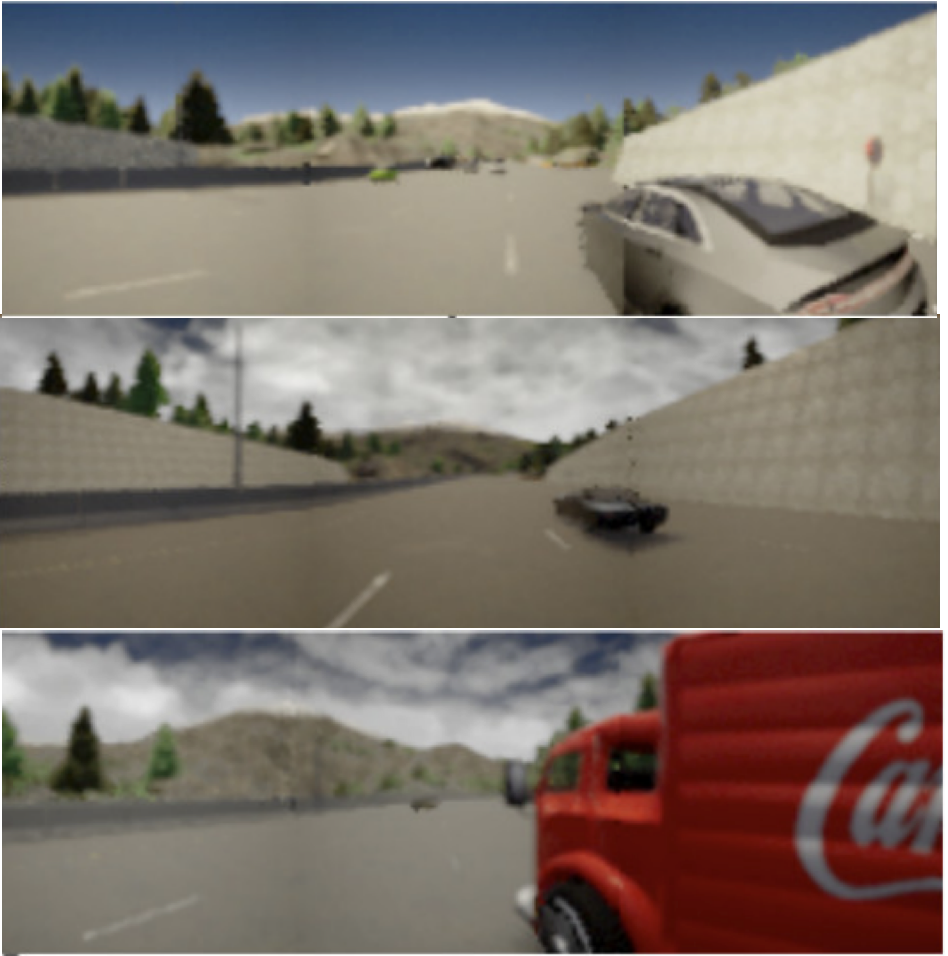
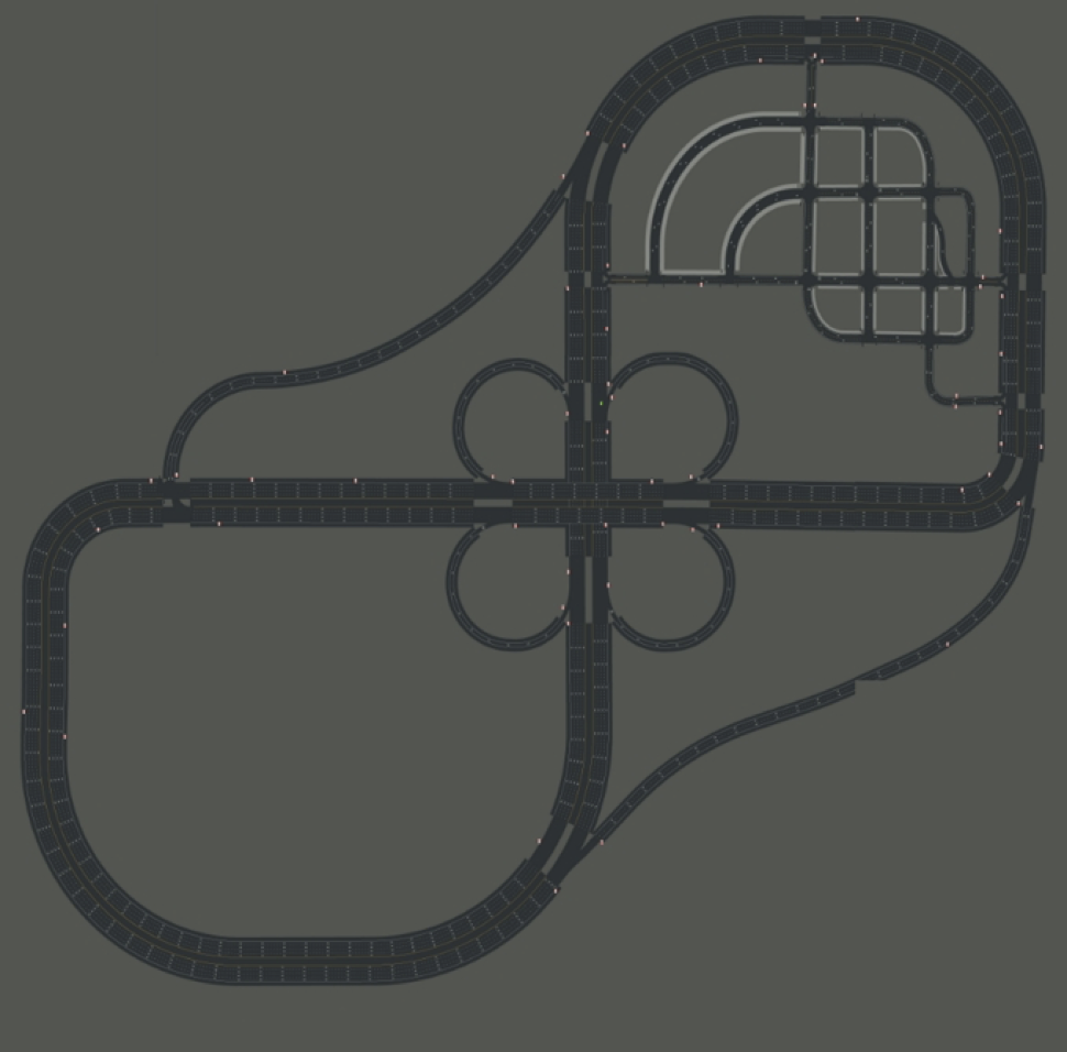
Refer to caption
(a)
Refer to caption
(b)
Figure 5: Sample egocentric view in CARLA environment on Town04 highway map. The highway layout is also shown

Table 6 summarizes the results, for these experiments DrQ was not used. Unlike the results reported in (Zhang et al., 2020), we observe that the minor adjustments we made to the architecture are enough to fully close the performance gap between SAC and the bisimulation-based options. The lack of result differentiation in Table 6 suggests that the original architecture was not well suited for the task, and bisimulation acted as a helpful regularization objective.

SAC DBC ϵbold-italic-ϵ\bm{\epsilon}-R PSE ϵbold-italic-ϵ\bm{\epsilon}-π𝜋\bm{\pi}
𝟏𝟔𝟖±𝟗plus-or-minus1689\bm{168\pm 9} 160±7plus-or-minus1607160\pm 7 157±11plus-or-minus15711157\pm 11 158±11plus-or-minus15811158\pm 11 148±23plus-or-minus14823148\pm 23
Table 6: Episodic reward on CARLA’s Town04 highway map, 500k500𝑘500k environment steps. Mean and standard deviation are computed across 5 seeds.