The Power of First-Order Smooth Optimization for Black-Box Non-Smooth Problems

Abstract

Gradient-free/zeroth-order methods for black-box convex optimization have been extensively studied in the last decade with the main focus on oracle call complexity. In this paper, besides the oracle complexity, we focus also on iteration complexity, and propose a generic approach that, based on optimal first-order methods, allows to obtain in a black-box fashion new zeroth-order algorithms for non-smooth convex optimization problems. Our approach not only leads to optimal oracle complexity, but also allows to obtain iteration complexity similar to first-order methods, which, in turn, allows to exploit parallel computations to accelerate the convergence of our algorithms. We also elaborate on extensions for stochastic optimization problems, saddle-point problems, and distributed optimization.

1 Problem Formulation

We consider optimization problem

$$\min_{x\in Q\subseteq\mathbb{R}^{d}}f(x)$$ (1)

in the setting of a zeroth-order oracle. This means that an oracle returns the value $f(x)$ at a requested point $x$ [13], possibly with some adversarial noise that is uniformly bounded by a small value $\Delta>0$. Let $\gamma>0$ be a small number to be defined later and $Q_{\gamma}:=Q+B^{d}_{2}(\gamma)$, where $B^{d}_{2}(\gamma)$ is the Euclidean ball with center at $0$ and radius $\gamma>0$ in $\mathbb{R}^{d}$. Using these objects, we make the following assumptions.

• The set $Q$ is convex and the function $f$ is convex on the set $Q_{\gamma}$;

• The function $f$ is Lipschitz-continuous with constant $M$, i.e. $|f(y)-f(x)|\leq M\|y-x\|_{p}$ on $Q_{\gamma}$, where $p\in[1,2]$ and $\|\cdot\|_{p}$ is the $p$-norm. If $p=2$ we use the notation $M_{2}$ for the Lipschitz constant.

This class of problems was widely investigated and optimal algorithms in terms of the number of zeroth-order oracle calls were developed in non-smooth setting [57, 19, 32, 67, 4] and smooth setting [57, 25, 38]. At the same time, to the best of our knowledge, the development of optimal algorithms in terms of the number of iterations is still an open research question [19, 10]. The goal of this paper is to propose a generic approach that allows us to construct algorithms with the best iteration complexity among the algorithms that have optimal oracle complexity. This can be seen as a two-criteria optimization problem if one would like to improve both: oracle complexity and iteration complexity. An important observation of this paper is that there is no need to sacrifice oracle complexity to obtain better iteration complexity. A special focus is made on the possibility to use non-Euclidean geometry to define the algorithms.
The simplest and most illustrative result obtained in this work is as follows. Our generic approach allows to solve problem (1) in the Euclidean geometry in $O(d^{1/4}M_{2}R/\varepsilon)$ successive iterations, each requiring $O(d^{3/4}M_{2}R/\varepsilon)$ oracle calls per iteration that can be made in parallel to make the total working time smaller. The dependence $\sim d^{1/4}/\varepsilon$ corresponds to the first part of the lower bound for iteration complexity [17, 10] $\min\left\{d^{1/4}\varepsilon^{-1},d^{1/3}\varepsilon^{-2/3}\right\}$. Note that this lower bound is obtained for a wider class of algorithms that allow $\text{Poly}\left(d,\varepsilon^{-1}\right)$ oracle calls per iteration. On the contrary, our algorithm makes minimal possible number of oracle calls in each iteration in such a way that the total number of oracle calls is optimal.
Due to the page limitation, we next describe the main results and technical details are deferred to the Appendices.

2 Smoothing Scheme

In this section we describe our main scheme that allows us to develop batch-parallel gradient-free methods for non-smooth convex problems based on batched-gradient algorithms for smooth stochastic convex problems. In the following sections, we generalize this scheme to non-smooth stochastic convex optimization problems and convex-concave saddle-point problems, including the problems with finite-sum structure.
The first element of our approach is the randomized smoothing for non-smooth objective $f$. This approach is rather standard, and goes back to 1970s [27, 53, 70]. The smooth approximation to $f$ is defined as the function

$$f_{\gamma}(x)=\mathbb{E}_{u}f(x+u),$$

where $u\sim RB^{d}_{2}(\gamma)$, i.e. $u$ is random vector uniformly distributed on $B^{d}_{2}(\gamma)$. The following theorem is a generalization of the results [78, 18] for non-Euclidean norms.

Theorem 2.1 (properties of $f_{\gamma}$).

For all $x,y\in Q$, we have

• $f(x)\leq f_{\gamma}(x)\leq f(x)+\gamma M_{{\color[rgb]{0,0,0}2}}$;

• $f_{\gamma}(x)$ is $M$-Lipschitz:

  $$|f_{\gamma}(y)-f_{\gamma}(x)|\leq M\|y-x\|_{p};$$

• $f_{\gamma}(x)$ has $L=\dfrac{\sqrt{d}M}{\gamma}$-Lipschitz gradient:

  $$\|\nabla f_{\gamma}(y)-\nabla f_{\gamma}(x)\|_{q}\leq L\|y-x\|_{p},$$

  where $q$ us such that $1/p+1/q=1$.

See Appendix A.6 for the proof.
The second very important element of our approach goes back to [67], who proposes a special unbiased stochastic gradient for $f_{\gamma}$ with small variance:

$$\nabla f_{\gamma}(x,e)=d\frac{f(x+\gamma e)-f(x-\gamma e)}{2\gamma}e,$$ (2)

where $e\sim RS^{d}_{2}(1)$ is a random vector uniformly distributed on $S^{d}_{2}(1)$ – Euclidean unit sphere with center at $0$ in $\mathbb{R}^{d}$. To simplify the further derivations, here and below we make a slight abuse of notation and denote by $f$ the value returned by the oracle, which can be an approximation to the value of the objective up to a small error, bounded by $\Delta$.

We note that an alternative way to define a stochastic approximation to $\nabla f_{\gamma}(x)$ is based on the double smoothing technique of B. Polyak [60, 4]. This approach is more complicated and requires stronger assumptions on the noise $\Delta$ (see Theorem 2.2). Thus, we use the approach of [67].

The following theorem is a combination of the results from [67, 40, 6].

Theorem 2.2 (properties of $\nabla f_{\gamma}(x,e)$).

For all $x\in Q$, we have

• $\nabla f_{\gamma}(x,e)$ is an unbiased approximation for $\nabla f_{\gamma}(x)$: $\mathbb{E}_{e}\left[\nabla f_{\gamma}(x,e)\right]=\nabla f_{\gamma}(x)$;

• $\nabla f_{\gamma}(x,e)$ has bounded variance (second moment):

  $$\mathbb{E}_{e}\left[\|\nabla f_{\gamma}(x,e)\|^{2}_{q}\right]\leq\kappa(p,d)\cdot\left(dM_{2}^{2}+\dfrac{d^{2}\Delta^{2}}{\gamma^{2}}\right),$$

  where $1/p+1/q=1$ and

  $$\kappa(p,d) =O\left(\sqrt{\mathbb{E}_{e}\|e\|_{q}^{4}}\right)={\color[rgb]{0,0,0}O\left(\min\left\{q,\ln d\right\}d^{2/q-1}\right)}$$

  $$=\begin{cases}O(1),\;p=2~{}{\color[rgb]{0,0,0}(q=2)}\\ O\left((\ln d)/d\right),\;p=1~{}{\color[rgb]{0,0,0}(q=\infty)}.\end{cases}$$

  Moreover, if $\Delta$ is sufficiently small, then

  $$\mathbb{E}_{e}\left[\|\nabla f_{\gamma}(x,e)\|^{2}_{q}\right]\leq 2\kappa(p,d)dM_{2}^{2}.$$

See Appendix A.7 for the proof.

Remark 2.3.

If the zeroth-order oracle returns an unbiased noisy stochastic function value $f(x,\xi)$ ($\mathbb{E}_{\xi}f(x,\xi)=f(x)$), then with two-point oracle we can introduce the following counterpart of (2)

$$\nabla f_{\gamma}(x,\xi,e)=d\frac{f(x+\gamma e,\xi)-f(x-\gamma e,\xi)}{2\gamma}e.$$ (3)

Theorem 2.2 remains valid with the appropriate changes of $\nabla f_{\gamma}(x,e)$ to $\nabla f_{\gamma}(x,\xi,e)$, the expectation $\mathbb{E}_{e}$ to the expectation $\mathbb{E}_{e,\xi}$, and the redefinition of $M_{2}$ as a constant satisfying $\mathbb{E}_{\xi}\|\nabla_{x}f(x,\xi)\|_{2}^{2}\leq M^{2}_{2}$ for all $x\in Q_{\gamma}$.

Based on the two elements above, we are now in a position to describe our general approach, which for shortness, we refer to as the Smoothing scheme (technique).
Assume that we have some batched algorithm A($L,\sigma^{2}$) that solves problem (1) under the assumption that $f$ is smooth and satisfies

$$\|\nabla f(y)-\nabla f(x)\|_{q}\leq L\|y-x\|_{p},\;\forall x,y\in Q_{\gamma},$$ (4)

and by using a stochastic first-order oracle that depends on a random variable $\eta$ and returns at a point $x$ an unbiased stochastic gradient $\nabla_{x}f(x,\eta)$ with bounded variance:

$$\mathbb{E}_{\eta}\left[\|\nabla_{x}f(x,\eta)-\nabla f(x)\|^{2}_{q}\right]\leq\sigma^{2}.$$ (5)

Further, we assume that, to reach $\varepsilon$-suboptimality in expectation, this algorithm requires $N(L,\varepsilon)$ successive iterations and $T(L,\sigma^{2},\varepsilon)$ stochastic first-order oracle calls, i.e. A($L,\sigma^{2}$) allows batch-parallelization with the average batch size $B(L,\sigma^{2},\varepsilon)=T(L,\sigma^{2},\varepsilon)/N(L,\varepsilon)$.
Our approach consists of applying A($L,\sigma^{2}$) to the smoothed problem

$$\min_{x\in Q\subseteq\mathbb{R}^{d}}f_{\gamma}(x)$$ (6)

with

$$\gamma=\varepsilon/(2M_{{\color[rgb]{0,0,0}2}})$$ (7)

and $\eta=e$, $\nabla_{x}f(x,\eta)=\nabla f_{\gamma}(x,e)$, where $\varepsilon>0$ is the desired accuracy for solving problem (1) in terms of the suboptimality expectation.
According to Theorem 2.1, an $(\varepsilon/2)$-solution to (6) is an $\varepsilon$-solution to the initial problem (1). According to Theorem 2.1 and (7) we have

$$L\leq\frac{2\sqrt{d}MM_{{\color[rgb]{0,0,0}2}}}{\varepsilon},$$ (8)

and, according to Theorem 2.2, we have

$$\sigma^{2}\leq 2\kappa(p,d)dM_{2}^{2}$$ (9)

if $\Delta$ is sufficiently small.
Thus, we obtain that A($L,\sigma^{2}$) implemented using stochastic gradient (2) is a zeroth-order method for solving non-smooth problem (1). Moreover, to solve problem (1) with accuracy $\varepsilon>0$ this method suffices to make

$$N\left(\frac{2\sqrt{d}MM_{{\color[rgb]{0,0,0}2}}}{\varepsilon},\varepsilon\right)\;\text{ successive iterations and }$$

$$2T\left(\frac{2\sqrt{d}MM_{{\color[rgb]{0,0,0}2}}}{\varepsilon},2\kappa(p,d)dM_{2}^{2},\varepsilon\right)\;\text{ zeroth-order oracle calls. }$$

We underline that this approach is flexible and generic as we can take different algorithms as A($L,\sigma^{2}$). For example, if we take batched Accelerated gradient method [14, 48, 15, 24, 37], then from (8), (9) we have that

$N(L,\varepsilon)=O\left(\sqrt{\frac{LR^{2}}{\varepsilon}}\right)=O\left(\frac{d^{1/4}{\color[rgb]{0,0,0}\sqrt{MM_{2}}}R}{\varepsilon}\right),$ $T(L,\sigma^{2},\varepsilon)=\tilde{O}\left(\max\left\{N(L,\varepsilon),\frac{\sigma^{2}R^{2}}{\varepsilon^{2}}\right\}\right)$ $=\tilde{O}\left(\frac{\kappa(p,d)dM_{2}^{2}R^{2}}{\varepsilon^{2}}\right),$

where $\tilde{O}\left(\,\cdot\,\right)$ is a convergence rate up to a logarithmic factor Here $R=O(\|x^{0}-x_{*}\|_{p}\ln d)$ with $x^{0}$ being the starting point and $x_{*}$ being the solution to (1) closest to $x^{0}$. The last equality assumes also that $\varepsilon\lesssim d^{-1/4}M_{2}^{{\color[rgb]{0,0,0}3/2}}R/M^{{\color[rgb]{0,0,0}1/2}}$ when $p=1$.

Theorem 2.4.

Based on the batched Accelerated gradient method, the Smoothing scheme applied to non-smooth problem (1), provides a gradient-free method with

$$O\left(\frac{d^{1/4}{\color[rgb]{0,0,0}\sqrt{MM_{2}}}R}{\varepsilon}\right)\;\text{ successive iterations and}$$

$$\tilde{O}\left(\frac{\kappa(p,d)dM_{2}^{2}R^{2}}{\varepsilon^{2}}\right)=\begin{cases}\tilde{O}\left(\frac{dM_{2}^{2}R^{2}}{\varepsilon^{2}}\right),\;p=2\\ \tilde{O}\left(\frac{(\ln d)M_{2}^{2}R^{2}}{\varepsilon^{2}}\right),\;p=1.\end{cases}$$

zeroth-order oracle calls.

See Appendix A.8 for the proof.

Next we make several remarks on some related works. First, an important difference between our Smoothing scheme and the work of [19] is that, unlike them we do not assume the smoothness of the objective $f$ and we use a different finite-difference approximation (2) due to [67]. Second, in [64], the authors use a similar smoothing technique to reduce the number of communications in distributed non-smooth convex optimization algorithms. Unlike their exact first-order oracle setting, we consider zeroth-order oracle model and construct stochastic approximation to the gradient of the smoothed function. Finally, the authors of [10] propose a close technique with an accelerated higher-order method [56, 31, 1] playing the role of A($L,\sigma^{2}$). For the particular setting of $p=2$, they obtain a better in some regimes bound $N\sim d^{1/3}/\varepsilon^{2/3}$ for the number of iterations. Yet, they have significantly worse oracle complexity $T$, which makes it unclear how to use their results in practice. To sum up, despite some similarities with other works, the proposed Smoothing scheme is, to the best of our knowledge, new, general, and flexible. Moreover, as we show below it is quite universal and can be applied to many different problems.

3 Applications Of the Smoothing Scheme

3.1 Stochastic Optimization

Based on Remark 2.3, we can consider the non-smooth stochastic convex optimization problem:

$$\min_{x\in Q\subseteq\mathbb{R}^{d}}\left\{f(x):=\mathbb{E}_{\xi}f(x,\xi)\right\}$$ (10)

with a two-point zeroth-order oracle that returns the values $\{f(x_{i},\xi)\}_{i=1}^{2}$ given two points $x_{1},x_{2}$. The result of Theorem 2.4 still holds if $M_{2}$ is redefined to be a constant satisfying $\mathbb{E}_{\xi}\|\nabla_{x}f(x,\xi)\|_{2}^{2}\leq M^{2}_{2}$ for all $x\in Q_{\gamma}$, $\eta$ is set to be the pair $(\xi,e)$. $e$ and $\xi$ are independent between iterations with available samples. Moreover, by using the stochastic gradient clipping [36], we can prove a stronger result and guarantee $\varepsilon$-suboptimality with high-probability (with exponential concentration) independently of distribution of $\nabla_{x}f(x,\xi)$.

If the two-point feedback as in (3) is not available, our Smoothing technique can utilize the one-point feedback by using the unbiased estimate [53, 29, 32]:

$$\nabla f_{\gamma}(x,\xi,e)=d\frac{f(x+\gamma e,\xi)}{\gamma}e,$$

with [32]

$$\mathbb{E}_{\xi,e}\left[\|\nabla f_{\gamma}(x,\xi,e)\|^{2}_{q}\right]\leq\begin{cases}\frac{(q-1)d^{1+2/q}G^{2}}{\gamma^{2}},\;q\in[2,2\ln d]\\ \frac{4d(\ln d)G^{2}}{\gamma^{2}},\;q\in(2\ln d,\infty),\end{cases}$$

where $\gamma$ is defined in (7) and it is assumed that $\mathbb{E}_{\xi}\left[|f(x,\xi)|^{2}\right]\leq G^{2}$ for all $x\in Q_{\gamma}$. Thus, the Smoothing technique can be generalized to the one-point feedback setup by replacing the RHS of (9) by the above estimate. This leads to the same iteration complexity $N$, but increases the oracle complexity $T$, and, consequently, the batch size $B$ at each iteration.

3.2 Finite-sum Problems

As a special case of (10) with $\xi$ uniformly distributed on $1,...,m$, we can consider the finite-sum (Empirical Risk Minimization) problem

$$\min_{x\in Q\subseteq\mathbb{R}^{d}}f(x):=\mathbb{E}_{\xi}f(x,\xi)=\frac{1}{m}\sum_{k=1}^{m}f_{k}(x).$$ (11)

Clearly, if we have incremental zeroth-order oracle, i.e. zeroth-order oracle for each $f_{k}$, we are in the setting of two-point feedback in the sense of Section 3.1. Thus, we can apply Theorem 2.4, where $M_{2}$ is defined as $\max_{k=1,...,m}\|\nabla f_{k}(x)\|_{2}\leq M_{2}$ for all $x\in Q_{\gamma}$.

At the same time, problem (11) has specific structure, that allows to split batching among nodes (to make algorithm centralized distributed among $m$ nodes) if batch size

$$B=\frac{T}{N}\simeq\frac{dM_{2}^{2}R^{2}/\varepsilon^{2}}{d^{1/4}M_{2}R/\varepsilon}=d^{3/4}\frac{M_{2}R}{\varepsilon}$$

is greater than $m$, i.e. $m\lesssim d^{3/4}M_{2}R/\varepsilon$. As it is known, in Machine Learning applications $m$ can be as large as $O\left(dM_{2}^{2}R^{2}/\varepsilon^{2}\right)$ [69, 28] or $O\left(M_{2}^{2}R^{2}/\varepsilon^{2}\right)$, if a proper regularization is applied [66, 65]. In both cases $m$ can be very large.

So, in this case ($d^{3/4}M_{2}R/\varepsilon\lesssim m\lesssim d^{3/2}M_{2}^{2}R^{2}/\varepsilon^{2}$), to preserve the total oracle complexity one can use stochastic Accelerated Variance Reduced algorithms [50, 47, 46, 49] with (see (8), (9))

$N(L,\varepsilon)=\tilde{O}\left(m+\sqrt{\frac{mLR^{2}}{\varepsilon}}\right)=O\left(\frac{d^{1/4}\sqrt{m}M_{2}R}{\varepsilon}\right),$ $T(L,\sigma^{2},\varepsilon)=\tilde{O}\left(\max\left\{N(L,\varepsilon),\frac{\sigma^{2}R^{2}}{\varepsilon^{2}}\right\}\right)=$ $=\tilde{O}\left(\frac{dM_{2}^{2}R^{2}}{\varepsilon^{2}}\right).$

The number of successive iterations grows, but now $m$-nodes distribution of batching is possible if

$$m\lesssim B=\frac{T}{N}\simeq\frac{dM_{2}^{2}R^{2}/\varepsilon^{2}}{d^{1/4}\sqrt{m}M_{2}R/\varepsilon}=d^{3/4}\frac{M_{2}R}{\sqrt{m}\varepsilon},$$

that is

$$m\lesssim d^{3/2}\frac{M_{2}^{2}R^{2}}{\varepsilon^{2}}.$$

This regime is quite natural for Machine Learning and Statistical applications [65, 68].
The results of this subsection can be generalized to the stochastic optimization problems with $f_{k}(x):=\mathbb{E}_{\xi}f_{k}(x,\xi)$, see (Section 3.1).

3.3 Strongly Convex Problems

By using the restart technique [53, 43] we can prove a counterpart of Theorem 2.4 for the case when $f$ is $\mu$-strongly convex w.r.t. the $p$-norm for some $p\in[1,2]$ and $\mu\geq\varepsilon/R^{2}$.

Theorem 3.1.

Based on the batched Accelerated gradient method, the Smoothing scheme applied to non-smooth and strongly convex problem (1), provides a gradient-free method with $\tilde{O}\left(\frac{d^{1/4}{\color[rgb]{0,0,0}\sqrt{MM_{2}}}}{\sqrt{\mu\varepsilon}}\right)$ successive iterations and $\tilde{O}\left(\frac{\kappa(p,d)dM_{2}^{2}}{\mu\varepsilon}\right)$ zeroth-order oracle calls, where $\kappa(p,d)$ is bounded as in Theorem 2.4.
Moreover, the same holds for stochastic optimization problem (10) if $M_{2}$ is defined as $\mathbb{E}_{\xi}\|\nabla_{x}f(x,\xi)\|_{2}^{2}\leq M^{2}_{2}$ for all $x\in Q_{\gamma}$.

See Appendix A.10 for the proof.

3.4 Saddle-point Problems

In this subsection we consider non-smooth convex-concave saddle-point problem

$$\min_{x\in Q_{x}\subseteq\mathbb{R}^{d_{x}}}\max_{y\in Q_{y}\subseteq\mathbb{R}^{d_{y}}}f(x,y).$$ (12)

Gradient-free methods for convex-concave saddle-point problems were studied in [8, 7, 34, 63] with the main focus on the complexity in terms of the number of zeroth-order oracle calls. Unlike these papers, we focus here also on the iteration complexity.

Applying Smoothing technique separately to $x$-variables and $y$-variables, we obtain almost the same results as for optimization problems with the only difference in Theorem 2.1: instead of

$$f(x)\leq f_{\gamma}(x)\leq f(x)+\gamma M_{{\color[rgb]{0,0,0}2}}$$

we have

$$f(x{\color[rgb]{0,0,0},y})-\gamma_{y}M_{{\color[rgb]{0,0,0}2,}y}\leq f_{\gamma}(x{\color[rgb]{0,0,0},y})\leq f(x{\color[rgb]{0,0,0},y})+\gamma_{x}M_{{\color[rgb]{0,0,0}2,}x}.$$

This leads to a clear counterpart of (7) for choosing $\gamma=\left(\gamma_{x},\gamma_{y}\right)$, where $M_{{\color[rgb]{0,0,0}2,}x}$, $M_{{\color[rgb]{0,0,0}2,}y}$ – corresponding Lipschitz constants in $2$-norm.

If we take as A($L,\sigma^{2}$) the batched Mirror-Prox or the batched Operator extrapolation method or the batched Extragradient method [41, 44, 35], using (8), (9), we obtain the following bounds

$N(L,\varepsilon)=O\left(\frac{LR^{2}}{\varepsilon}\right)=O\left(\frac{\sqrt{d}{\color[rgb]{0,0,0}MM_{2}}R^{2}}{\varepsilon^{2}}\right),$ $T(L,\sigma^{2},\varepsilon)=O\left(\max\left\{N(L,\varepsilon),\frac{\sigma^{2}R^{2}}{\varepsilon^{2}}\right\}\right)$ $=O\left(\frac{\kappa(p,d)dM_{2}^{2}R^{2}}{\varepsilon^{2}}\right),$

where $d=\max\{d_{x},d_{y}\}$, $M_{2}=\max\left\{M_{2,x},M_{2,y}\right\}$, $R$ depends on the criteria. For example, if $\varepsilon$ is expected accuracy in fair duality gap [41], then $R$ is a diameter in $p$-norm of $Q_{x}\otimes Q_{y}$ up to a $\ln d$-factor, where $\otimes$ is a Cartesian product of two sets. The last equality assumes that $d\lesssim(M_{2}/M)^{{\color[rgb]{0,0,0}2}}$ when $p=1$. This result is also correct for stochastic saddle-point problems with proper redefinition of what is $M_{2}$, see Section 3.1.
We see that due to the lack of acceleration for saddle-point problems the batch-parallelization effect is much more modest than for convex optimization problems.
By using the restart technique we can generalize these results to $\mu$-strongly convex, $\mu$-strongly concave case, see Section 3.3. Alternatively, we can combine the Smoothing technique with Stochastic Accelerated Primal-Dual method from [81] for (12) with $f(x,y)$ being $\mu_{x}$-strongly convex and $\mu_{y}$-strongly concave in $2$-norm (Euclidean setup). In this case we obtain the following bounds

$N(\{L\},\varepsilon)=\tilde{O}\left(\frac{L_{xx}}{\mu_{x}}+\frac{\max\left\{L_{xy},L_{yx}\right\}}{\sqrt{\mu_{x}\mu_{y}}}+\frac{L_{yy}}{\mu_{y}}\right)$ $=\tilde{O}\left(\frac{\sqrt{d_{x}}M_{2,x}^{2}}{\mu_{x}\varepsilon}+\frac{M_{2,x}M_{2,y}\max\left\{\sqrt{d_{x}},\sqrt{d_{y}}\right\}}{\sqrt{\mu_{x}\mu_{y}}\varepsilon}+\frac{\sqrt{d_{y}}M_{2,y}^{2}}{\mu_{y}\varepsilon}\right),$ $T(\{L\},\{\sigma^{2}\},\varepsilon)=\tilde{O}\left(\max\left\{N(\{L\},\varepsilon),\frac{\sigma_{x}^{2}}{\mu_{x}\varepsilon}+\frac{\sigma_{y}^{2}}{\mu_{y}\varepsilon}\right\}\right)$ $=\tilde{O}\left(\frac{d_{x}M_{2,x}^{2}}{\mu_{x}\varepsilon}+\frac{d_{y}M_{2,y}^{2}}{\mu_{y}\varepsilon}\right),$

where we use subscripts corresponding to $x$ or $y$ variables, e.g. $L_{xx},L_{xy},L_{yx},L_{yy}$ is defined as

$$\|\nabla_{x}f_{\gamma}(x_{2},y)-\nabla_{x}f_{\gamma}(x_{1},y)\|_{2}\leq L_{xy}\|x_{2}-x_{1}\|_{2}$$

$$\|\nabla_{x}f_{\gamma}(x,y_{2})-\nabla_{x}f_{\gamma}(x,y_{1})\|_{2}\leq L_{xy}\|y_{2}-y_{1}\|_{2}$$

$$\|\nabla_{y}f_{\gamma}(x_{2},y)-\nabla_{y}f_{\gamma}(x_{1},y)\|_{2}\leq L_{yx}\|x_{2}-x_{1}\|_{2}$$

$$\|\nabla_{y}f_{\gamma}(x,y_{2})-\nabla_{y}f_{\gamma}(x,y_{1})\|_{2}\leq L_{yy}\|y_{2}-y_{1}\|_{2}$$

for all $(x,y)\in Q_{x,\gamma_{x}}\otimes Q_{y,\gamma_{y}}$. The only non-trivial calculation here is estimation of $L_{xy}$, $L_{yx}$, see Appendix A.9 for the proof. The other constants $\{L\}$ and $\{\sigma^{2}\}$ are defined according to the standard Smoothing scheme with variables $x$ or $y$ corresponding to subscripts.
Note, that most of the results for saddle-point problems (i.e. mentioned result from [81] or finite-sum composite generalization [75]) with different constants of smoothness and strong convexity/concavity were obtained based on the Accelerated gradient method for convex problems and Catalyst envelope, that allows us to generalize it to saddle-point problems [52]. There exist also loop-less (direct) accelerated methods that save $\ln(\varepsilon^{-1})$-factor in the complexity, for $\mu_{x}$-strongly convex, $\mu_{y}$-strongly concave saddle-point problems [45]. But even for composite bilinear saddle-point problems (with different smoothness and strong convexity constants) there is still a gap between the state-of-the-art upper bounds [45] and lower bounds [80].

3.5 Distributed Optimization

In decentralized distributed convex optimization and convex-concave saddle-point problems optimal methods (both in terms of communication rounds and oracle calls) were developed in the Euclidean setup, see, e.g. surveys [39, 20]. In particular, there exists a batched-consensus-projected Accelerated gradient method [62] that, for $\mu$-strongly convex in $2$-norm $f$ from (11) with $L$-Lipschitz gradient in $2$-norm, requires

$$N(L,\varepsilon)=\tilde{O}\left(\sqrt{\chi\frac{L}{\mu}}\right)=\tilde{O}\left(\frac{\sqrt{\chi}d^{1/4}M_{2}}{\sqrt{\mu\varepsilon}}\right)$$

communication rounds and

$$T(L,\sigma^{2},\varepsilon)=\tilde{O}\left(\max\left\{N(L,\varepsilon),\frac{\sigma^{2}}{\mu\varepsilon^{2}}\right\}\right)=\tilde{O}\left(\frac{dM_{2}^{2}}{\mu\varepsilon}\right)$$

oracle calls per node, where $M_{2}$ is defined in Section 3.2, $\chi$ – condition number of the Laplace matrix of communication network or square of worst-case condition number for time-varying networks [62].
This batched-consensus-projected Accelerated gradient method is optimal (up to a $\ln(\varepsilon^{-1})$-factor) as a decentralized method, but the Smoothing technique provides a gradient-free method that is not the best (state-of-the-art) method in terms of communication rounds. The best one requires $\tilde{O}\left(\sqrt{\chi}M_{2}/\sqrt{\mu\varepsilon}\right)$ communication rounds [6]. This holds for stochastic decentralized convex problems with two-point feedback and one-point feedback. For the one-point feedback, optimal decentralized method is described in [71]. This method is better also by a $\sim d^{1/4}$-factor in terms of the number of communication rounds.
For saddle-point problems, by replacing in the Smoothing scheme the batched-consensus Accelerated gradient method [62], which is optimal for decentralized convex problems, with the batched-consensus Extragradient method [9], which is optimal for decentralized convex-concave saddle-point problems, we lose a $\sim\sqrt{d}$-factor in the number of communication rounds in comparison with optimal gradient-free methods for non-smooth decentralized saddle-point problems.
To sum up, in distributed optimization, for the first time, we have a situation where the Smoothing scheme generates a non-optimal method from an optimal one.

4 Discussion

4.1 Superposition Of Different Techniques

In convex optimization and convex-concave saddle-point problems there are several generic techniques that allow black-box reduction of known methods to develop new methods for new problem classes [30]. For example, the Restart technique mentioned in Section 3.3 allows to construct methods for strongly convex problems based on methods for convex problems; the Catalyst envelope mentioned in Section 3.4 allows to construct methods for convex-concave saddle-point problems based on methods developed for convex optimization problems; Batching technique mentioned in Section 2 allows to construct methods for stochastic problems based on methods developed for deterministic problems; Consensus-projection technique mentioned in Section 3.5 allows to build decentralized distributed methods for convex problems based on non-decentralized methods developed for non-decentralized convex problems.
The first important property of all these reduction techniques, informally speaking, is that all of them preserve the optimality of the method: an optimal method after applying any of the techniques becomes optimal [30] for the new class of problems. We remark that the Catalyst envelope leads to optimal algorithms only on a certain (yet large enough) class of problems, see Section 3.4 for details. Also, when considering saddle-point problems with different strong convexity constants, it is better to use a direct method rather than the Restart technique. Despite these limitations, the optimality-preserving property is very useful in practice.
The second important property is that a superposition or different combination of these reduction techniques also preserves the optimality of algorithms. This can be demonstrated via the batched-consensus-projected Accelerated gradient method from Section 3.5. This algorithm is obtained via a combination of the Batching technique and the Consensus-projection technique applied to Accelerated gradient method. Moreover, the Restart technique can be added to this combination in order to obtain the algorithm for strongly convex problems.
Note that in some cases these techniques require a proper generalization before they can be applied as a part of combination. For example, when we generalize the batched-consensus-projected Accelerated gradient method to saddle-point problems, instead of the standard Catalyst envelope developed in this context in [52], we should use a special decentralized stochastic (batched) version of the Catalyst envelope, that can be developed from [46, 74].
We expect that the Smoothing scheme (technique) developed in this paper will take its rightful place in the mentioned above (not exhaustive) list of useful reduction techniques that allow us to develop new methods based on existing ones.
In the previous (sub)sections we demonstrated that the Smoothing scheme is quite generic and allows a black box reduction of algorithms for smooth problems to solve non-smooth problems. Moreover, except the combination with Consensus-projection technique, the Smoothing scheme allows to obtain optimal algorithms for non-smooth black-box problems with zeroth-order oracle. Thus, as one of our main contributions in this paper, we consider the observation that the Smoothing scheme can be developed in a such a way, that it can be used in different combinations with other reduction techniques.

4.2 Batching Technique

In the Smoothing scheme an input algorithm should be a batched-gradient algorithm, and, thus, the Smoothing scheme strongly depends on the Batching technique, which we now describe in more detail. In Section 2 we mentioned some particular algorithms [14, 48, 15, 24] which do not constitute a generic technique that allows us to utilize an arbitrary algorithm, which solves a deterministic smooth convex problem. Some attempts to propose a generic Batching technique were made [23, 30] in a much more general setting of inexact models of the objective, which we do not consider here. Instead, we describe here a simple version in the convex case and for the Euclidean setting with $p=2$.
First of all, following [15, 23, 20] we introduce the notion of $(\delta_{1},\delta_{2},L)$-oracle. We say that for the problem (1) we have an access to $(\delta_{1},\delta_{2},L)$-oracle at a point $x$ if we can evaluate a vector $\nabla_{\delta}f(x)$ such that, for all $x,y\in Q_{\gamma}$,

$$-\delta_{1}\leq f(y)-f(x)-\langle\nabla_{\delta}f(x),y-x\rangle\leq\frac{L}{2}\|y-x\|_{2}^{2}+\delta_{2},$$

where $\mathbb{E}\delta_{1}=0$ ($\delta_{1}$ is independently taken at each oracle call), $\mathbb{E}\delta_{2}\leq\delta$. Note that the left inequality corresponds to the definition of $\delta_{1}$-(sub)gradient [60] and reduces to the convexity property in the case $\delta_{1}=0$. In this case the LHS holds with $\nabla_{\delta}f(x)=\nabla f(x)$. The right inequality in the case when $\delta_{2}=0$ is a consequence of (4). Let us consider an algorithm A($L,\delta_{1},\delta_{2}$) that converges with the rate

$$\mathbb{E}f(x^{N})-f(x_{*})=O\left(\frac{LR^{2}}{N^{\alpha}}+N^{\beta}\delta\right).$$ (13)

The batching technique, applied to the problem (10) with $L$-Lipschitz gradient (in 2-norm), is based on the use of the mini-batch stochastic approximation of the gradient

$$\nabla_{\delta}f(x)=\frac{1}{r}\sum_{j=1}^{r}\nabla_{x}f(x,\xi^{j})\\$$

in A($L,\delta_{1},\delta_{2}$), where $\{\xi^{j}\}_{j=1}^{r}$ are sampled independently and $r$ is an appropriate batch size. The choice of $r$ is based on the following relations

$$\langle\nabla_{\delta}f(x)-\nabla f(x),y-x\rangle\leq$$

$$\leq\frac{1}{2L}\|\nabla_{\delta}f(x)-\nabla f(x)\|_{2}^{2}+\frac{L}{2}\|y-x\|_{2}^{2},$$

$$\mathbb{E}_{\{\xi^{j}\}}\left[\|\nabla_{\delta}f(x)-\nabla f(x)\|_{2}^{2}\right]\leq\frac{\sigma^{2}}{r},$$

where $\sigma^{2}$ is the variance of $\nabla_{x}f(x,\xi)$, see (5). Hence, if

$$\delta\leq\frac{1}{2L}\max_{x\in Q_{\gamma}}\mathbb{E}_{\{\xi^{j}\}_{j=1}^{r}}\left[\|\nabla_{\delta}f(x)-\nabla f(x)\|_{2}^{2}\right],\;\text{i.e.}$$

$\delta=\frac{\sigma^{2}}{2Lr}$, we have that A($2L,\delta_{1},\delta_{2}$) converges with the rate given in (13). From (13) we see that to obtain

$$\mathbb{E}f(x^{N})-f(x_{*})\leq\varepsilon$$

it suffices to take

$$N=O\left(\left(\frac{LR^{2}}{\varepsilon}\right)^{1/\alpha}\right)\quad\text{and}\quad r=O\left(\frac{\sigma^{2}N^{\beta}}{L\varepsilon}\right).$$

In particular, for the Accelerated gradient method we have that $\alpha=2$, $\beta=1$ [15, 23]. In this case, we obtain the complexity bounds for batched Accelerated gradient methods mentioned in Section 2:

$N=O\left(\sqrt{LR^{2}/\varepsilon}\right)$, $B=r=O\left(\sigma^{2}R/\left(\sqrt{L}\varepsilon^{3/2}\right)\right)$, $T=N\cdot B=O\left(\sigma^{2}R^{2}/\varepsilon^{2}\right)$.

Note that, based on [72], the described above Batching technique can be applied to saddle-point problems. In particular, this allows to obtain new methods for stochastic bilinear saddle-point problems with composites based on the state-of-the-art method of [45]. The latter method, for the considered class of problems, works better than Stochastic Accelerated Primal-Dual method [81] which we use in Section 3.4.
Interestingly, our Smoothing scheme is not the only technique for reduction of algorithms for smooth convex problems to algorithms for non-smooth convex problems. Universal Nesterov’s technique from [55] claims that if $f$ is $M_{2}$-Lipschitz, then, for arbitrary $\delta>0$,

$$f(y)\leq f(x)+\langle\nabla f(x),y-x\rangle+\frac{L}{2}\|y-x\|_{2}^{2}+\delta,$$

with $L=M_{2}^{2}/(2\delta)$. Based on this observation, a generic reduction of algorithms with inexact gradient for smooth convex problems to algorithms for non-smooth problems is possible. Although it may seem that this approach combined with full gradient approximation by finite-differences [5] can be applied for our setting, it is not the case. Firstly, since $L=M_{2}^{2}/(2\delta)$ and for Accelerated gradient method $\delta$ should be such that $N\delta\simeq\varepsilon$, since $\beta=1$, we obtain that $L\sim\varepsilon^{-3/2}$, rather than $L\sim\varepsilon^{-1}$ that we have in our Smoothing scheme. Secondly, the full gradient approximation by finite-differences provably works for smooth objective $f$ [5], which is not our case.
Thus, the proposed Smoothing scheme is better than alternative approaches based on other smoothing techniques such as the Universal Nesterov’s technique [55], Nesterov’s smoothing via regularization of dual problem [54] and its different generalizations [16, 58, 76], which are designed and work good in the setting of first-order methods, but lead to inferior complexity in the zeroth-order setting. Unlike these approaches, our Smoothing scheme achieves the best known complexity in terms of the successive iterations number with the best possible number of zeroth-order oracle calls.

5 Experiments

5.1 Reinforcement learning

Reinforcement Learning (RL) is one of the key motivations for the proposed approach. We focus in this section on the Actor-Critic architecture and assume that the Critic is available to the Actor during training through a black-box oracle. This situation naturally motivates the application of zeroth-oder methods in which we only have access to function values. Moreover, the optimization problem is stochastic and may be convex or non-convex, smooth or non-smooth. Our RL experiments are carried out in the environment called "Reacher-v2," which is provided by the Open AI Gym toolkit. The network structure is described in Appendix A.2. We use PyTorch ADAM optimizer with three alternative inexact gradients for the Actor learning problem: exact gradient (Gradient), central finite difference (Central) from (2) and forward finite difference (Forward) defined as

$$\nabla f_{\gamma}(x,e)=d\frac{f(x+\gamma e)-f(x)}{\gamma}e.$$ (14)

For a better visualization, we plot the moving average of the reward with a window size of $250$. Figure 2 shows the convergence of our methods.

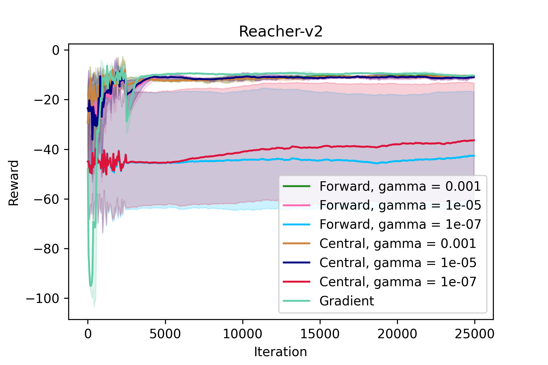
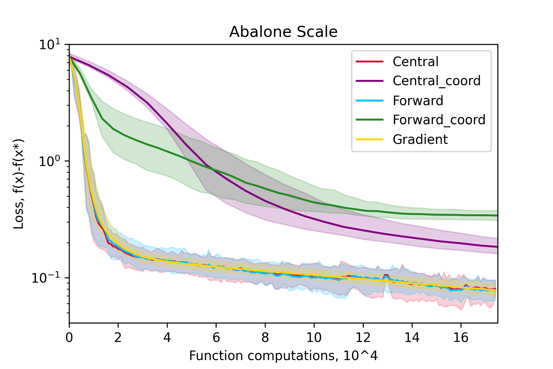
Figure 1: Actor’s reward for ADAM with Forward and Central differences for various $\gamma$ and exact gradient ADAM. lr= 1e-5.

Figure 2: Loss for abalone scale dataset with batch size $=100$, learning rate is $0.1$ and $\gamma=$1e-5.

5.2 Robust Linear Regression

Least absolute deviation (LAD) is a non-smooth convex problem, one of the variant of a robust linear regression [79]. It is more robust to outliers in data than the standard Linear Regression. The problem statement is

$$\min\limits_{w\in\mathbb{R}^{d}}\{f(w)=\tfrac{1}{n}\textstyle{\sum}_{k=1}^{m}|x_{i}^{T}w-y_{i}|\},$$ (15)

where $(x_{i},y_{i})$ are feature and target pairs. For the experiments we take simple dataset "abalone scale" from the LibSVM [11]. For this problem, we also implement ZO method with central coordinate and forward coordinate finite differences for the comparison. Their full definitions can be found in the Appendix A.3. Figure 2 shows the convergence of our methods.

5.3 Support Vector Machine

Support Vector Machine (SVM) is one of the classical classification algorithms that is still very popular. The problem statement is:

$$\min\limits_{w\in\mathbb{R}^{d}}\{f(w)=\tfrac{\mu}{2}\|w\|^{2}+\tfrac{1}{n}\textstyle{\sum}_{k=1}^{m}(1-y_{i}\cdot x_{i}^{T}w)_{+}\},$$ (16)

where $(x_{i},y_{i})$ are feature and label pairs. We use the LibSVM basic dataset "a9a" for our experiments with this problem. Figure 3 shows the convergence of our methods.

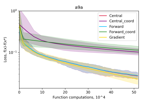
Figure 3: Loss for a9a dataset with $\mu=$1e-05, batch size $=100$, $lr=0.1$. $\gamma=$1e-5.

5.4 Conclusion on Experiments

We run experiments with $4$ different seeds ranging from $0$ to $3$ and present mean values as a main line and a light filling between the maximum and minimum values. The Figures 2, 2 and 3 show that with a decent choice of $\gamma$, ADAM with zeroth-order oracle works nearly as well as ADAM with exact gradient. Central and Forward differences outperform their coordinate versions, as it can be seen from Figures 2 and 3. The effect of computational instability appears for tiny $\gamma$ since $x$ is too close to $x+\gamma e$ and we reach the machine precision when computing the function value. However, Figure 2 demonstrates that the Central approximation is more robust than Forward to such errors since the distance between points is twice larger than in the Forward case. All these plots show that our approach is applicable and can compete with gradient-based methods. For more experiments, see Appendixes A.2, A.3, A.4.

Conclusion

This paper is devoted to the development of a universal smoothing scheme that allows us to construct efficient zeroth-order/gradient-free methods for non-smooth problems based on batched-gradient methods for smooth problems. This scheme preserves the efficiency of the input methods transferring it to the output zeroth-order method. Our smoothing scheme combines well with many other reduction techniques (batching, restarts, Catalyst acceleration for saddle-point problems, consensus-projection for decentralized distributed algorithms) that allows us to obtain via our scheme many algorithms for a wide class of non-smooth problems. As a future work we mention adaptive [21, 26] and inexact model [72] (composite, max-structure, etc.) generalizations. Another generalization consist in replacing $2$-sphere randomization on $1$-sphere randomization in smoothing scheme [33]. In some special regimes such randomization allows to improve complexity estimates on a logarithmic factor [2].

Appendix A Appendix

A.1 Additional Experiments: Adversarial Attack

Adversarial attack is aimed to generate input images with unobtrusive interference introduced to them to deceive a well trained classifier. These adversarial examples are created to recognize the robustness of models. In our experiments, we used ZO methods to generate adversarial examples targeted at a black-box model trained to solve a task of classification of MNIST dataset of handwritten digits. The output of this model is $F(\cdot)=[F_{1}(\cdot),\dots,F_{K}(\cdot)]$, where $F_{k}(\cdot)$ is a prediction score of the $k^{th}$ class. A correctly classified sample image $\mathbf{a_{i}}$ is taken from the dataset and its adversarial example is produced as follows:

$$\mathbf{a_{i}^{adv}}=0.5\tanh(\tanh^{-1}(2\mathbf{a_{i}})+\mathbf{x})$$ (17)

Next, we apply the same individual attacking loss utilized in [12]:

$$f_{i}(\mathbf{x})=\max\{\log F_{y_{i}}(\mathbf{a_{i}^{adv}})-\max_{t\neq y_{i}}\log F_{t}(\mathbf{a_{i}^{adv}}),0\}+\lambda\|\mathbf{a_{i}^{adv}}-\mathbf{a_{i}}\|^{2}$$ (18)

In our experiments we used sample images for digit class "1" and "4" and set their regularization parameters as $\lambda=1$ and $\lambda=0.1$ respectively.

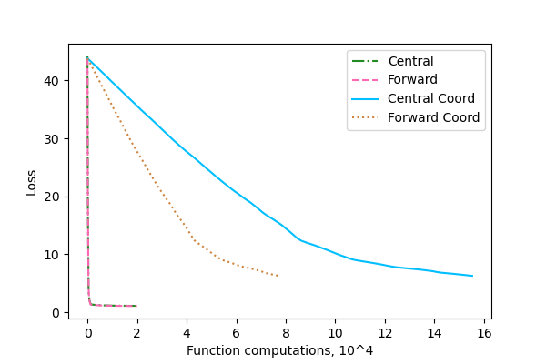
Figure 4: Comparison of different zeroth-order algorithms for generating $n=50$ adversarial examples for digit class "4" with $\lambda=0.1$. Left: Loss (18) with Central, Forward, Central Coord and Forward Coord where $lr=0.01$ and $\gamma=0.01$. Right: Distortion($\frac{1}{n}\sum_{i=1}^{n}\|\mathbf{a_{i}^{adv}}-\mathbf{a_{i}}\|^{2}$) average in $n=50$ generated adversarial examples.

Figure 4 shows that methods with coordinate steps require more function computations to converge which is justified by large $d$. This can also be observed in Table 1 where randomly generated adversarial examples were classified similarly by target model, although it is clear that each method produces different result.

All the experiments were conducted in Python 3 and PyTorch 1.10.1 on an Ubuntu 20.04.3 LTS machine with Intel(R) Xeon(R) Silver 4215 CPU @ 2.50GHz and 125 GB RAM.

Table 1: Generated adversarial examples for digit “1” class from a random batch of $n=10$ images, where image distortion is defined as $\frac{1}{n}\sum_{i=1}^{n}\|\mathbf{a}^{adv}_{i}-\mathbf{a}_{i}\|^{2}$.

Image ID $7$ $10$ $13$ $18$ $19$ $20$ $21$ $22$ $28$ $29$ Image distortion $\bf Original$ Central $5.0107$ Classified as $\bf 4$ $\bf 6$ $\bf 7$ $\bf 4$ $\bf 8$ $\bf 8$ $\bf 8$ $\bf 3$ $\bf 8$ $\bf 8$ Forward $5.1004$ Classified as $\bf 4$ $\bf 6$ $\bf 7$ $\bf 4$ $\bf 8$ $\bf 8$ $\bf 8$ $\bf 3$ $\bf 8$ $\bf 8$ Central Coord $4.6761$ Classified as $\bf 4$ $\bf 6$ $\bf 7$ $\bf 4$ $\bf 8$ $\bf 8$ $\bf 8$ $\bf 3$ $\bf 8$ $\bf 4$ Forward Coord $4.4163$ Classified as $\bf 4$ $\bf 6$ $\bf 7$ $\bf 4$ $\bf 8$ $\bf 8$ $\bf 8$ $\bf 3$ $\bf 8$ $\bf 8$

A.2 Additional Experiments: RL experiments

Our RL experiments are carried out in an environment called "Reacher-v2," which is provided by the Open AI Gym toolkit. This environment simulates an agent ($2$ DOF robotic arm) tasked with reaching a particular target (red sphere) in a 2D square space. The target is placed at random at the start of each episode. So, the action belongs to continuous space. Implementation of Deep Deterministic Policy Gradients (DDPG) algorithm from [51] is used to train the Actor-Critic agent. This policy $\pi\colon\mathcal{S}\to\mathcal{A}$ takes the state of a current environment and maps it to a predicted action. The Actor and Critic networks are made up of two hidden layers of fully-connected neural networks with $h_{1}=400$ and $h_{2}=300$ neurons with relu activation functions. To match the constraints of available actions, the Actor’s output is also scaled by tanh activation multiplied by the maximum allowed action.

Figure 5 shows the dependence of ZO methods on $\gamma$. One can see that: for a fitted learning rate $=0.0001$ at the right side of 5, methods converge for all $\gamma$; for a small learning rate =1e-5 at 2, methods converge for all $\gamma$ except the smallest $\gamma=$1e-7; for a big learning rate $=0.001$ at the left side of 5, Gradient method converges but all ZO methods collect errors and slowly diverge; for a huge learning rate $=0.01$ at the right side of 6, all methods diverge. As a result, we find a regime where ZO methods are stable and very close to gradient methods, but also, we find a regime where gradient method converges and ZO methods diverge. The left side of 6 shows that all gradient methods in our experiments converge to the same level. Figure 7 is made for a detailed look on regime with a huge learning rate $=0.01$ at the left side of 5.

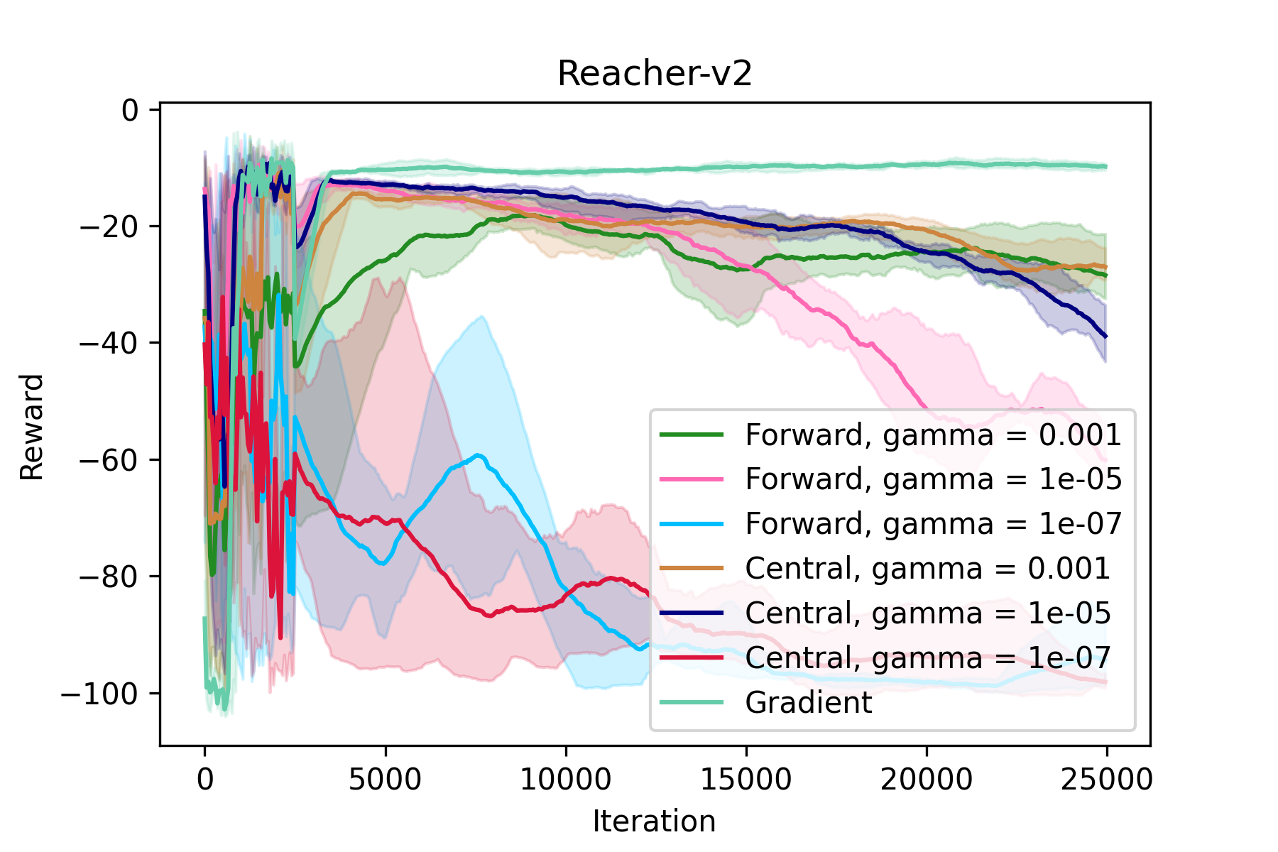
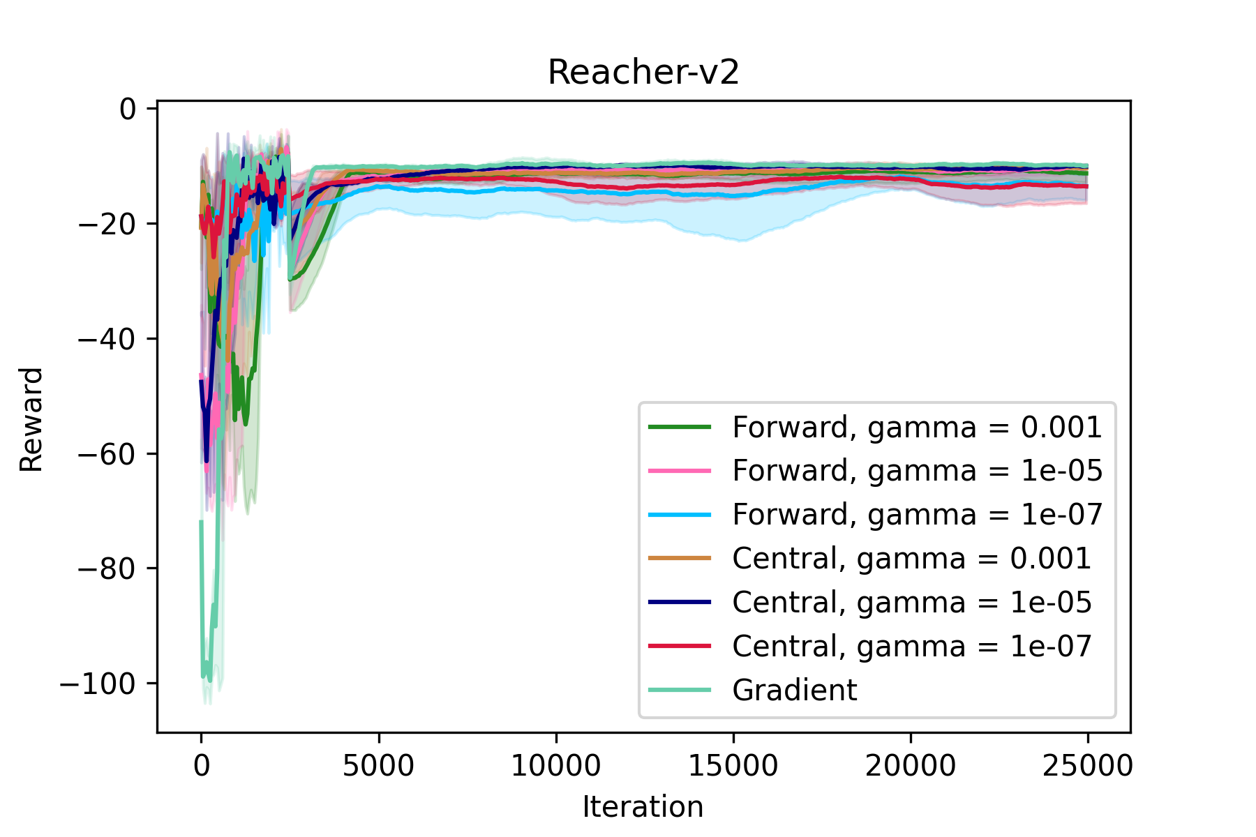
Figure 5: Left: Actor’s reward for ADAM with Forward and Central with various $\gamma$ and true gradient ADAM, where $lr=0.001$.
Right: Actor’s reward for ADAM with Forward and Central with various $\gamma$ and true gradient ADAM, where $lr=0.0001$.

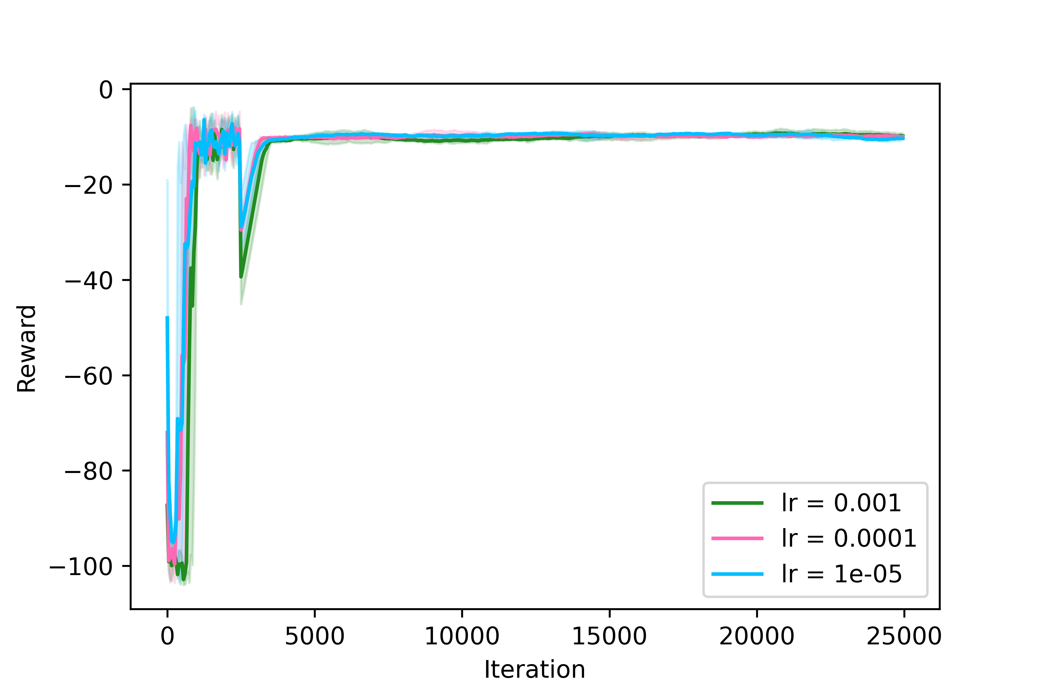
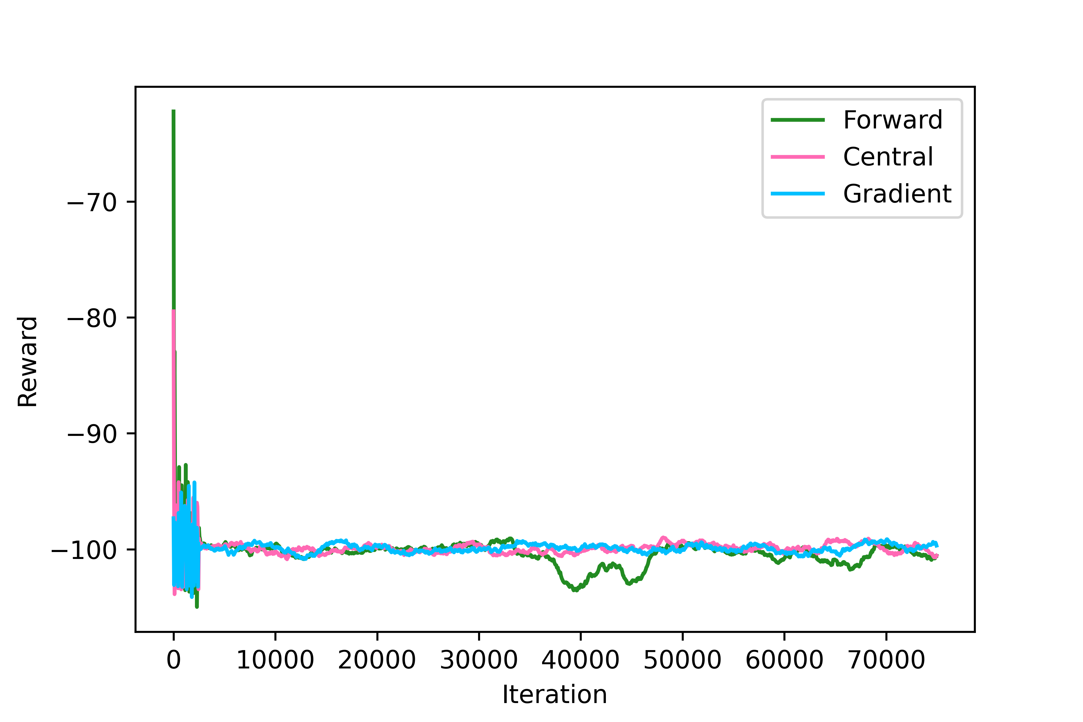
Figure 6: Left: Actor’s reward for true gradient ADAM with different learning rates.
Right: Actor’s reward for $25000$ iterations of ADAM with Forward and Central finite difference with various $\gamma=1e-5$ and true gradient ADAM, where $lr=0.01$.

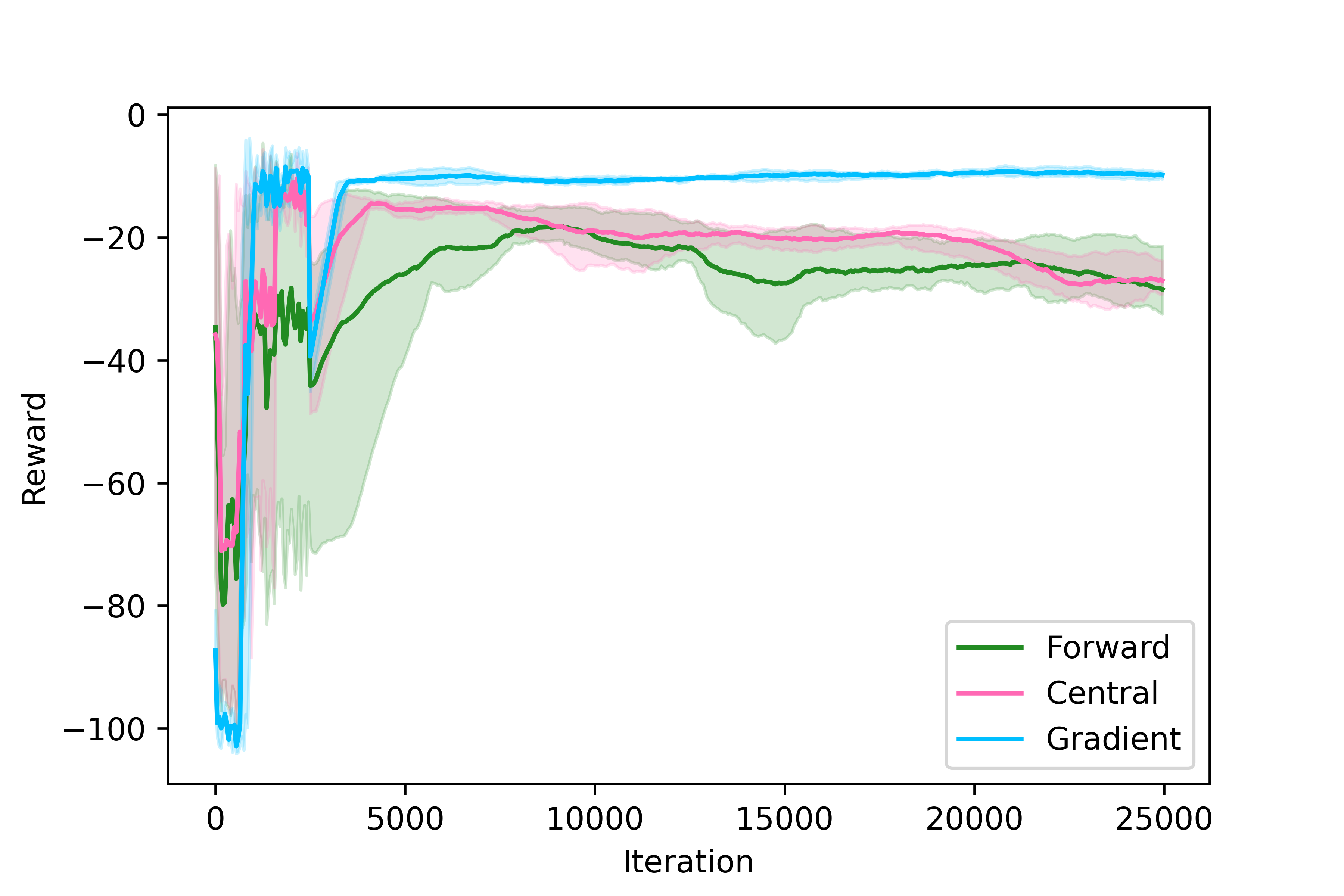
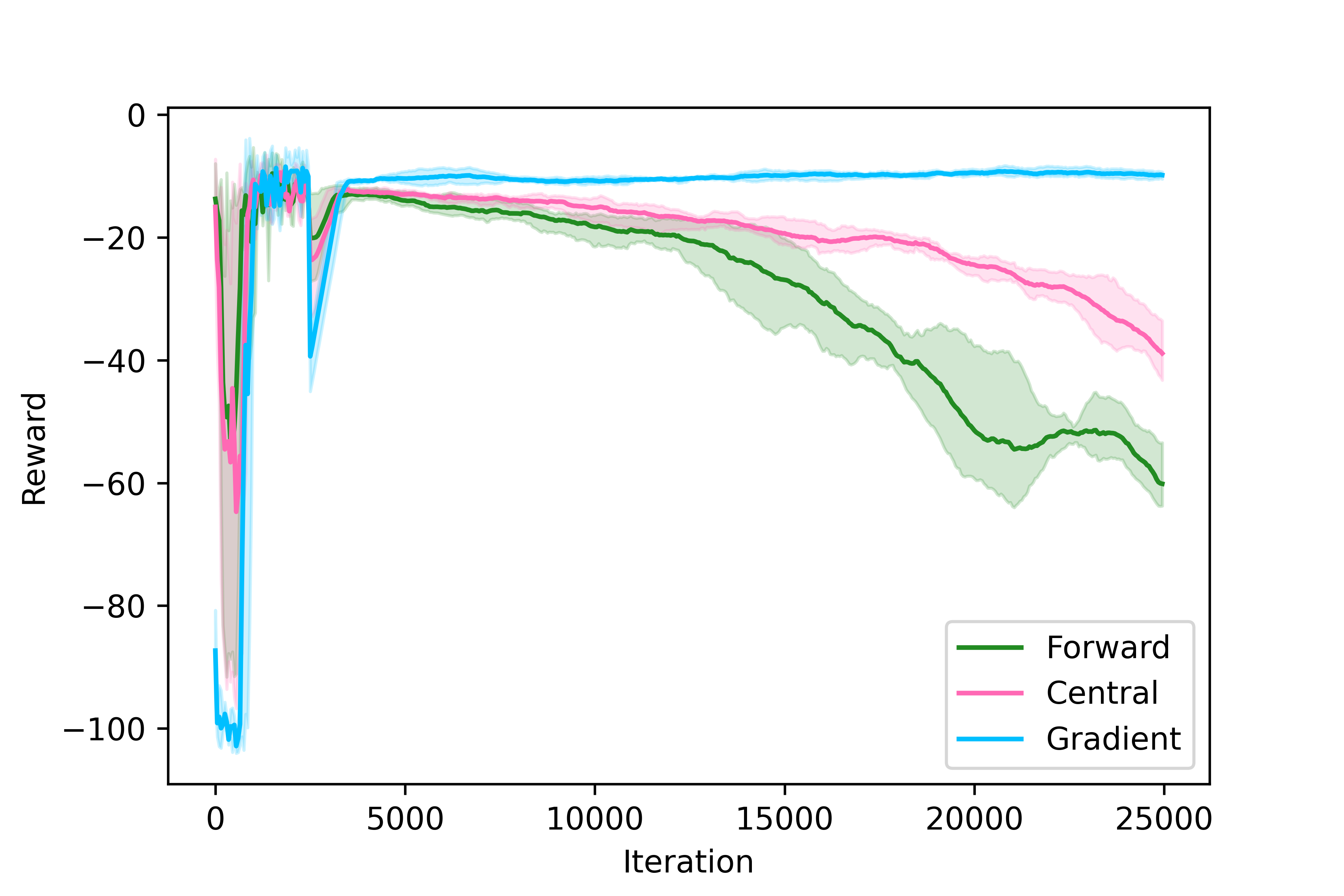
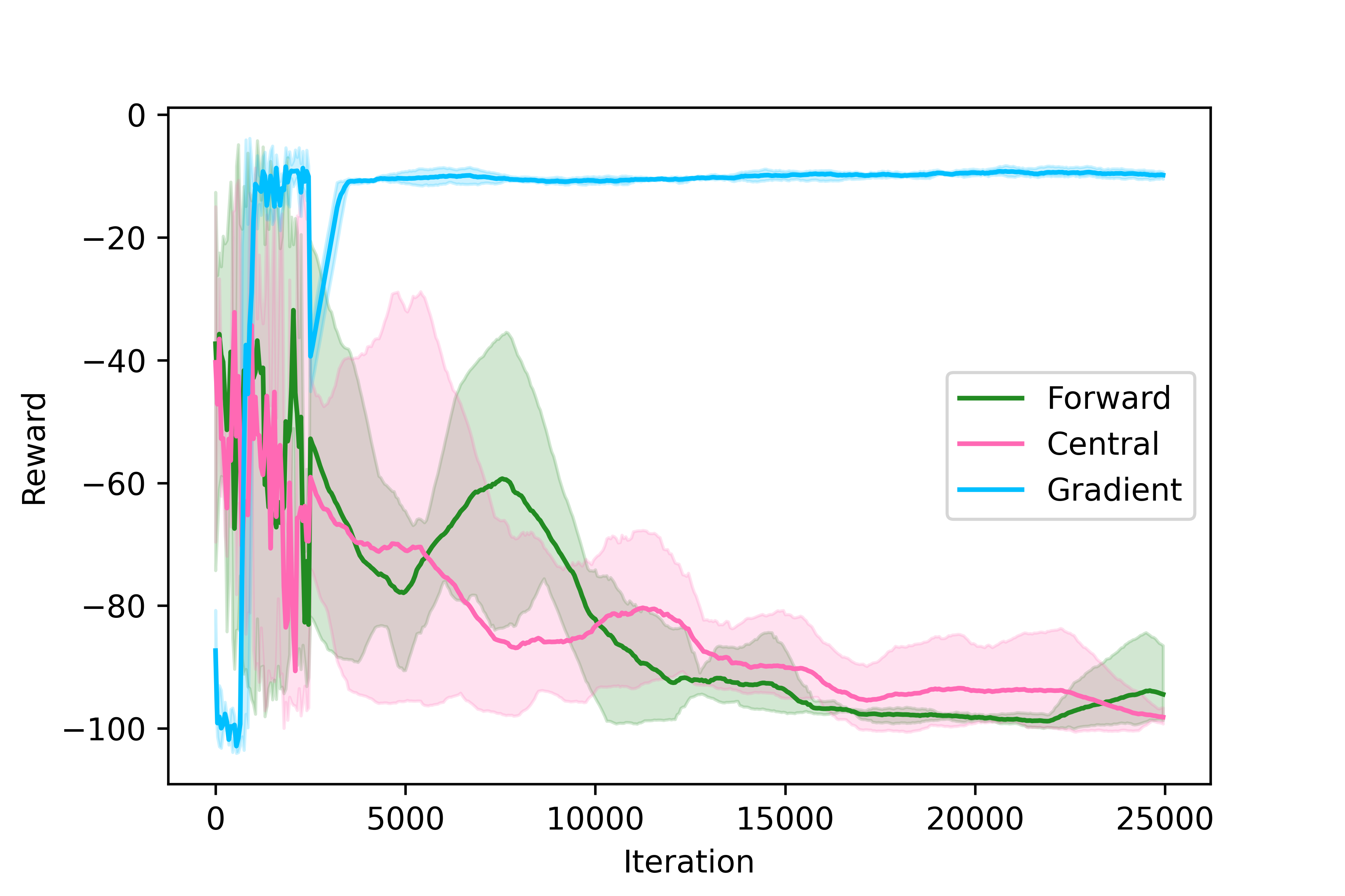
Figure 7: Left: Actor’s reward for ADAM with Forward and Central for $\gamma=1e-3$ and true gradient ADAM, where $lr=0.001$.
Middle: Actor’s reward for ADAM with Forward and Central for for $\gamma=1e-5$ and true gradient ADAM, where $lr=0.001$.
Right: Actor’s reward for ADAM with Forward and Central for $\gamma=1e-7$ and true gradient ADAM, where $lr=0.001$.

A.3 Additional Experiments: Robust Linear Regression

For the learning, we divide dataset "abalone scale" into two parts, where the part for training is $3500$ samples. The dimension of features equals to $8$. So, it is a very small dataset. We take dataset with such small dimension to compare Forward and Central with their variants of coordinate steps that depend on dimension.

The Central Coordinate is a zero-order finite difference such that we take (2) approximation $d$ times by each coordinate. Hence, we get $2d$ function computations per each step.

The Forward Coordinate is a zero-order finite difference such that we take (14) approximation $d$ times by each coordinate. Hence, we get $d+1$ function computations per each step.

As a result, coordinate steps are more accurate approximation of the gradient but also, they are more expansive computationally. We also add some graphics for Robust Linear Regression with different parameters.

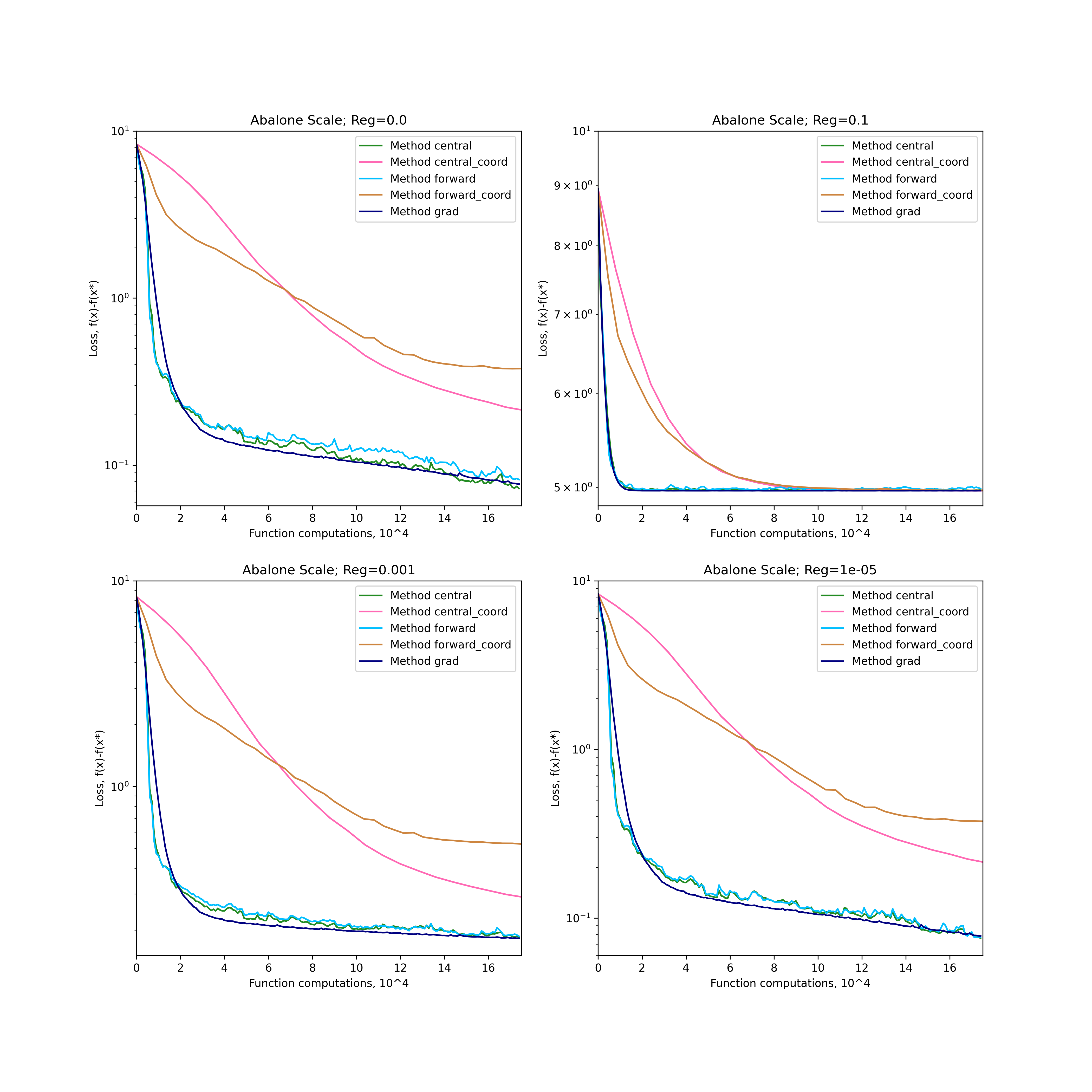
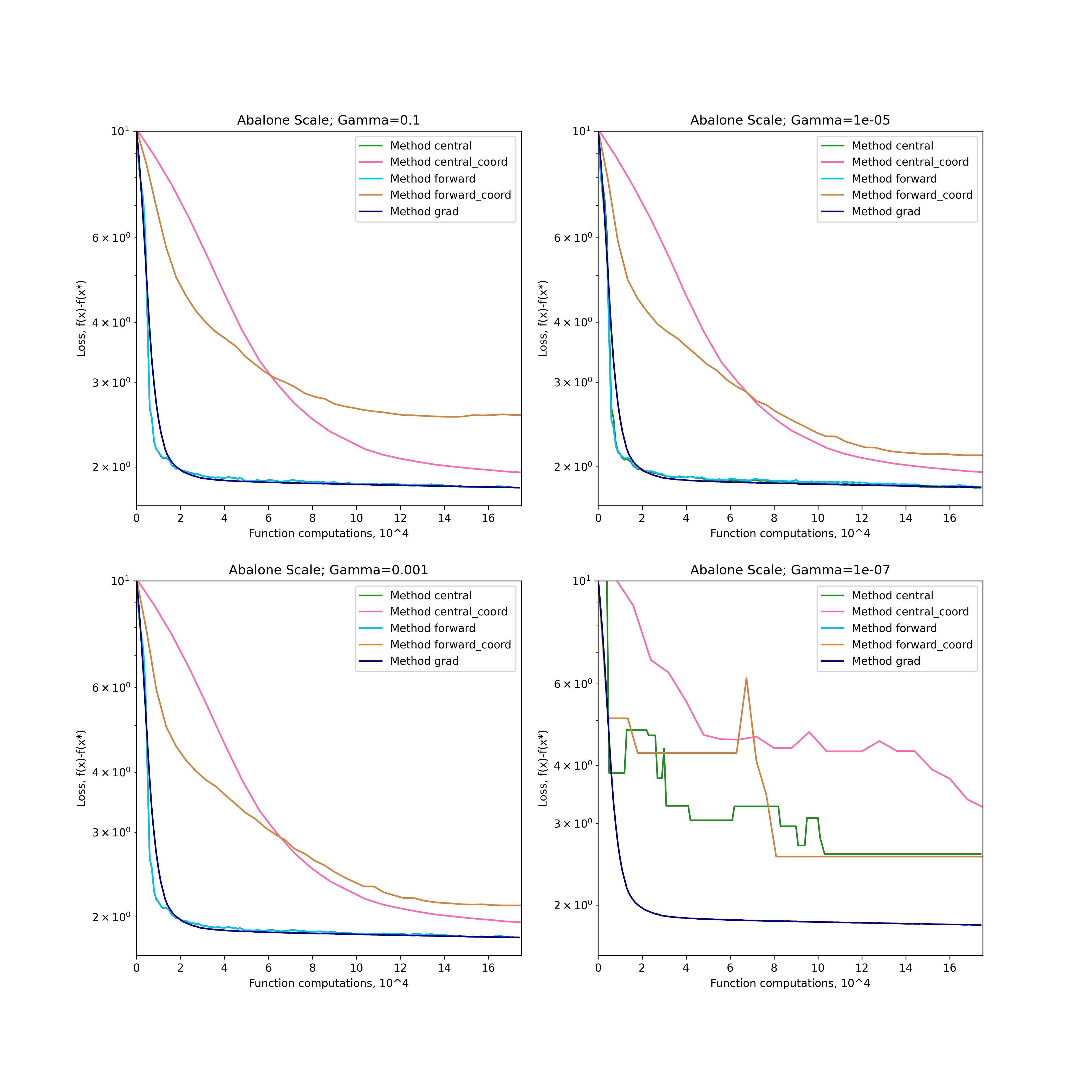
Figure 8: Left: Loss for abalone scale dataset with $lr=0.4$ batch size $=100$, $\gamma=$1e-5, and different $\mu$.
Right: Loss for abalone scale dataset with $lr=0.4$ batch size $=100$, $\mu=0.$ and different $\gamma$.

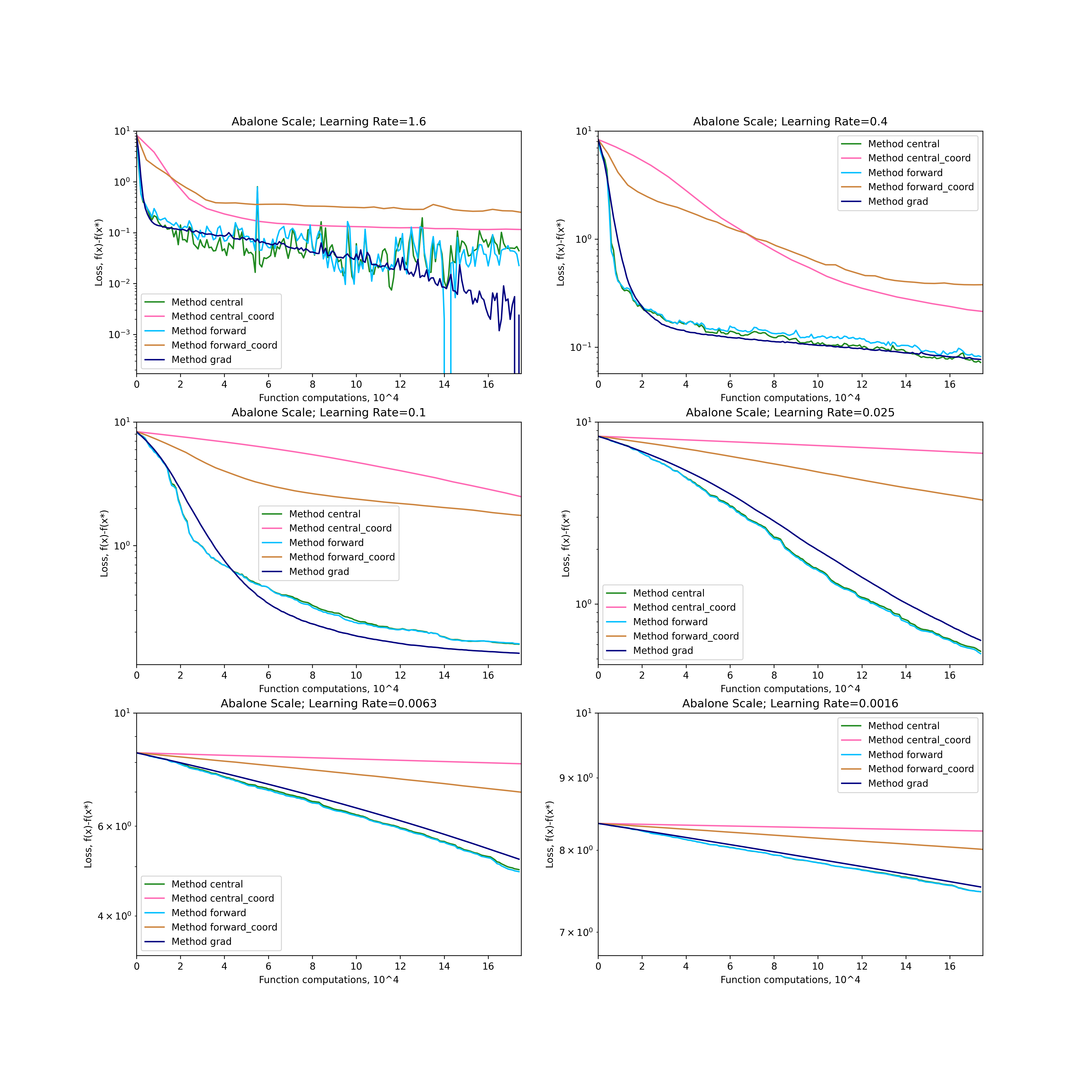
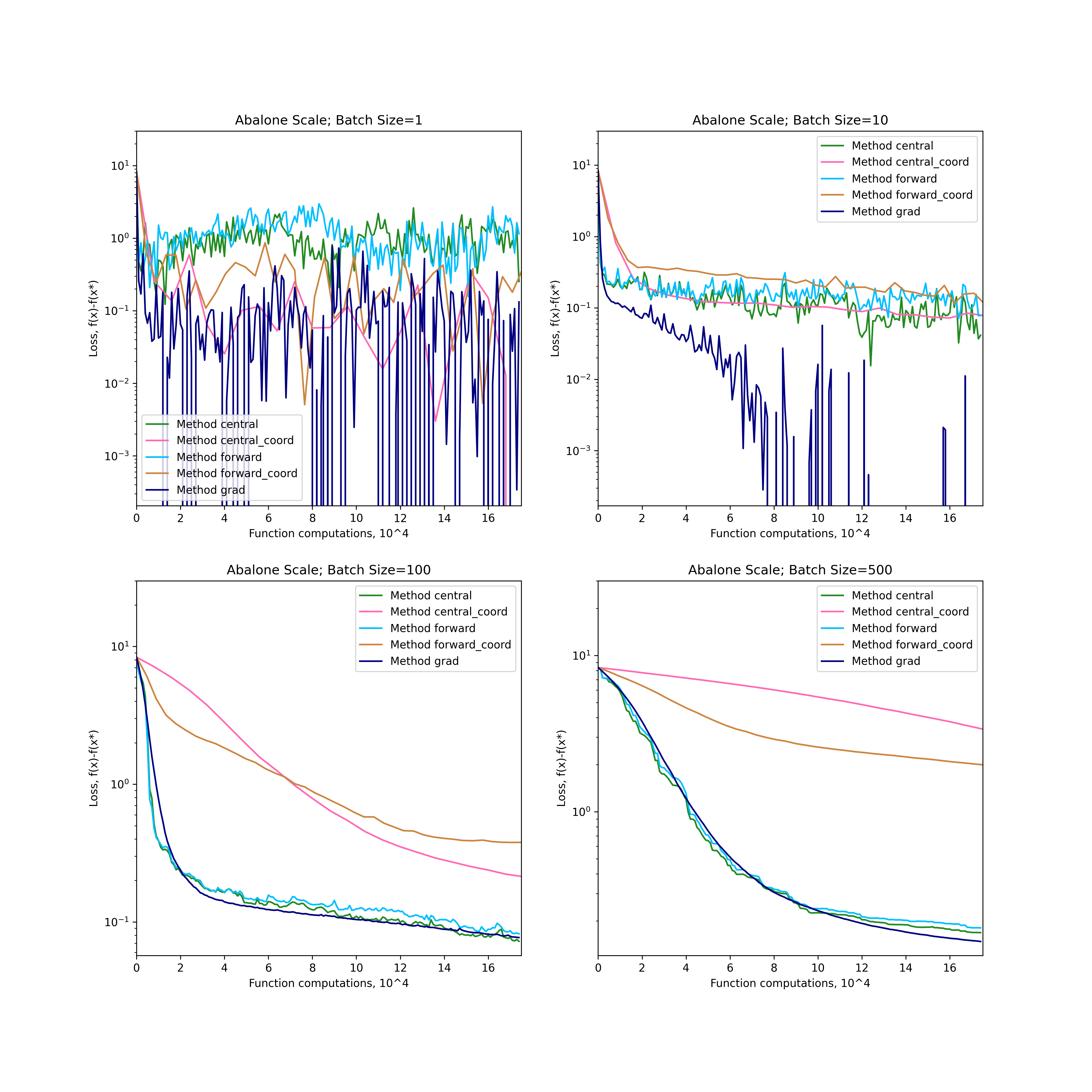
Figure 9: Left: Loss for abalone scale dataset with $lr=0.4$ batch size $=100$, $\gamma=$1e-5, and different $lr$.
Right: Loss for abalone scale dataset with $lr=0.4$, $\mu=0.$, $\gamma=$1e-5, and different batch size.

A.4 Additional Experiments: Support Vector Machine

In this subsection one can see additional graphics for SVM with different parameters.

Figure 10 compares performance of ZO methods for $a9a$ dataset with various $\gamma$ (Left) and learninng rates (Right). It can be observed (Left) that Central and Forward methods converge faster than Central Coordinate and Forward Coordinate methods. Also, it is clear that both pairs of Coordinate and Non-Coordinate methods converge in a similar fashion. However, under extreme cases of $\gamma$ some methods do not converge at all. For instance, Forward Coordinate method with $\gamma=0.1$, Central and Forward methods with $\gamma=1e^{-07}$. Comparison of ZO methods under different Learning rate values (Right) also supports the above-mentioned corollary that in general Central and Forward methods converge faster than Central Coordinate and Forward Coordinate methods. However, it can be seen that larger values of learning rate introduces variance to ZO methods, although considerably smaller than for true gradient. It is also worth noting that small learning rate values result Central and Forward methods to converge with the same rate.

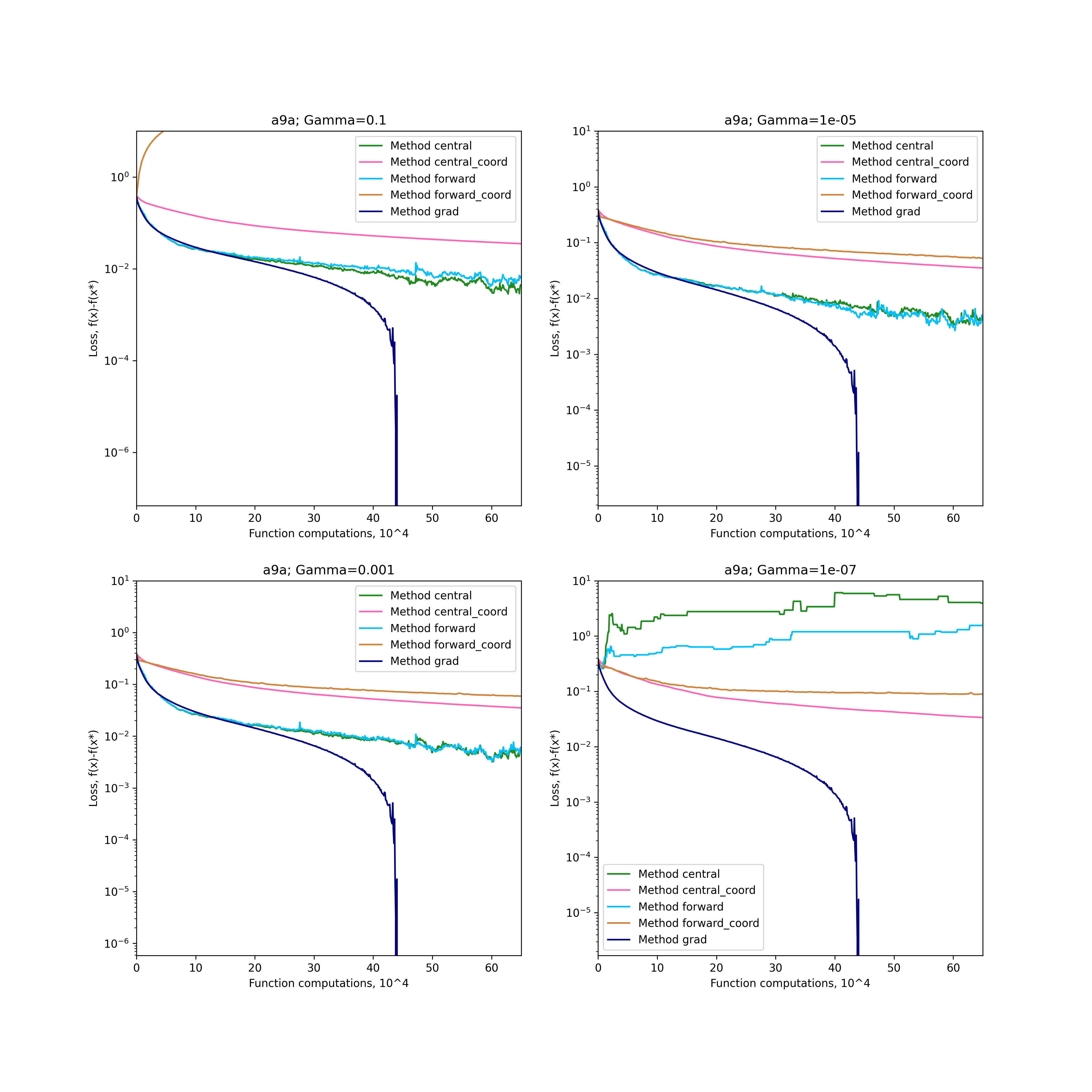
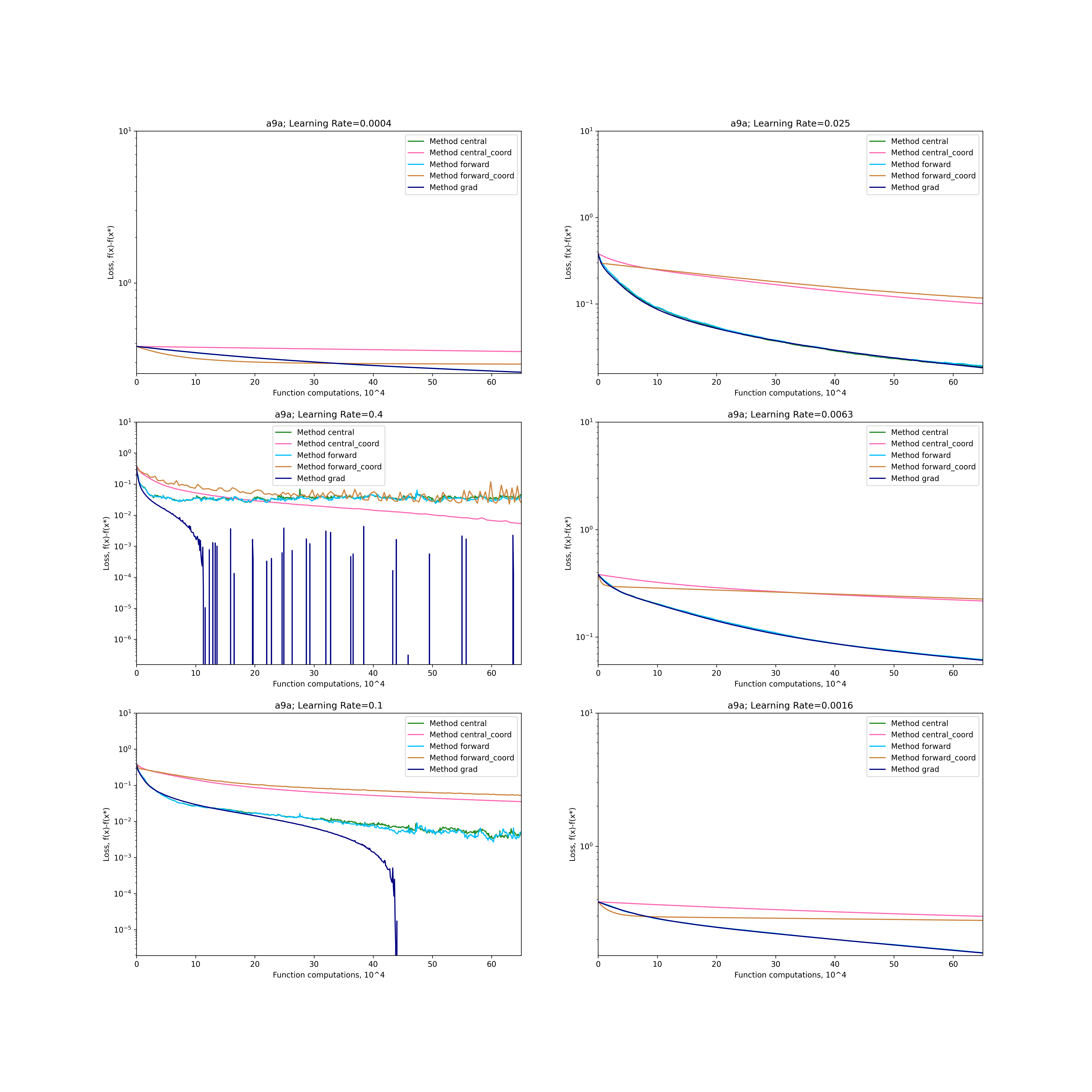
Figure 10: Left: Loss for a9a dataset with $\mu=1e-5$, batch size $=100$, $lr=0.1$ and different $\gamma$.
Right: Loss for a9a dataset with $\mu=1e-5$, batch size $=100$, $\gamma=$1e-5 and different $lr$.

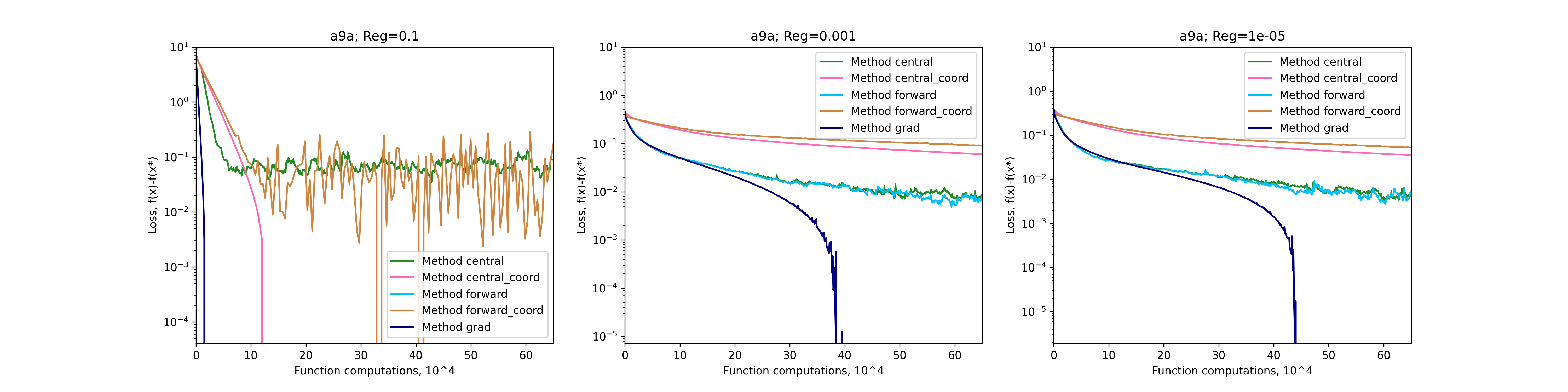
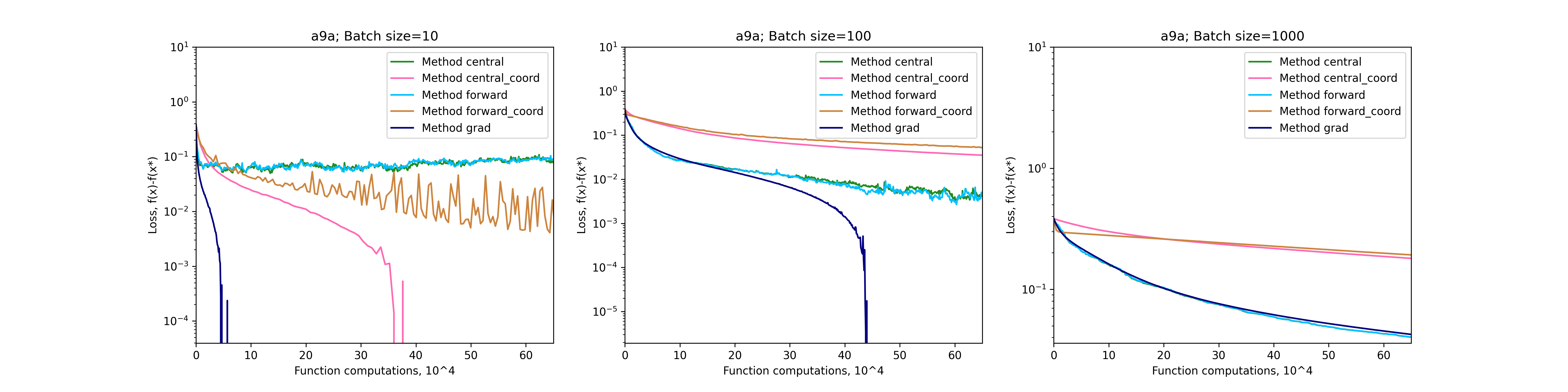
Figure 11: Loss for a9a dataset with $\mu=$1e-5, batch size $=100$, $lr=0.1$, $\gamma=$1e-5 and different $\mu$.

Figure 12: Loss for a9a dataset with $\mu=$1e-5, $lr=0.1$, $\gamma=$1e-5 and different batch size.

A.5 Reducing Variance Under Batching In $p$-norm

Lemma A.1.

If $\sigma$ is determined from

$$\mathbb{E}_{e\sim RS_{2}^{d}(1)}\left[\exp\left(\frac{\left\|d\dfrac{f(x+\gamma e)-f(x-\gamma e)}{2\gamma}e-\nabla f_{\gamma}(x)\right\|_{q}^{2}}{\sigma^{2}}\right)\right]\leq\exp(1),$$

then the variance of batched gradient

$$\sigma_{B}^{2}=\text{Var}\left[\nabla^{B}f_{\gamma}(x,\{e_{i}\}_{i=1}^{B})\right]\leq\dfrac{\sigma^{2}}{B}\cdot(2\chi(p,d)+\sqrt{3\pi\chi(p,d)}+3)=\dfrac{\sigma^{2}}{B}\lambda(p,d),$$

where $\chi(p,d)=\min{\left\{q-1,2\ln{d}\right\}}$, $\frac{1}{p}+\frac{1}{q}=1$.

Proof:

The batched gradient for the function $f_{\gamma}(x)=\mathbb{E}_{u}\left[f(x+\gamma u)\right]$ ($u\in RB_{2}^{d}(1)$) is:

$$\nabla^{B}f_{\gamma}(x,\{e_{i}\}_{i=1}^{B})=\frac{1}{B}\sum\limits_{i=1}^{B}\left[\dfrac{d}{2\gamma}\left(f(x+\gamma e_{i})-f(x-\gamma e_{i})\right)e_{i}\right],$$

where $e_{i}\in RS_{2}^{d}(1)$ are i.i.d.

For simplicity we denote $s_{i}=\left[\dfrac{d}{2\gamma}\left(f(x+\gamma e_{i})-f(x-\gamma e_{i})\right)e_{i}\right]$, so $\nabla^{B}f_{\gamma}(x,\{e_{i}\}_{i=1}^{B})=\dfrac{1}{B}\sum\limits_{i=1}^{B}s_{i}$, where $s_{i}$ are i.i.d. We denote $\overset{\circ}{s}_{i}=s_{i}-\mathbb{E}s_{i}$.

From Theorem $2.1$ from [42], we have

$$\mathbb{P}\left(\left\|\sum\limits_{i=1}^{B}\overset{\circ}{s}_{i}\right\|_{q}\geq\left(\sqrt{2\chi}+\sqrt{2}\beta\right)\sqrt{B}\sigma\right)\leq e^{-\beta^{2}/3},$$

where $\xi\leq\min{\left(2\ln{d},q-1\right)}$ (example $3.2$ from [42]), $q\geq 2$

$$\text{Var}\left[\nabla^{B}f_{\gamma}(x,\{e_{i}\}_{i=1}^{B})\right] = \mathbb{E}\left[\left\|\dfrac{1}{B}\sum\limits_{i=1}^{B}\overset{\circ}{s}_{i}\right\|_{q}^{2}\right]=\int\limits_{t=0}^{+\infty}\mathbb{P}\left(\left\|\dfrac{1}{B}\sum\limits_{i=1}^{B}\overset{\circ}{s}_{i}\right\|_{q}\geq\sqrt{t}\right)dt$$

$$=\int\limits_{t=0}^{2\chi B\sigma^{2}}\mathbb{P}\left(\left\|\dfrac{1}{B}\sum\limits_{i=1}^{B}\overset{\circ}{s}_{i}\right\|_{q}\geq\sqrt{t}\right)dt+\int\limits_{t=2\chi B\sigma^{2}}^{+\infty}\mathbb{P}\left(\left\|\dfrac{1}{B}\sum\limits_{i=1}^{B}\overset{\circ}{s}_{i}\right\|_{q}\geq\sqrt{t}\right)dt.$$

Substituting $\sqrt{t}=\left(\sqrt{2\chi}+\sqrt{2}\beta\right)\sqrt{B}\sigma$, we obtain:

$$\text{Var}\left[\nabla^{B}f_{\gamma}(x,\{e_{i}\}_{i=1}^{B})\right] \leq 2\chi B\sigma^{2}+\int\limits_{\beta=0}^{+\infty}\left[\mathbb{P}\left(\left\|\dfrac{1}{B}\sum\limits_{i=1}^{B}\overset{\circ}{s}_{i}\right\|_{q}\geq\left(\sqrt{2\chi}+\sqrt{2}\beta\right)\sqrt{B}\sigma\right)-2B\sigma^{2}(\sqrt{\chi}+\beta)\right]d\beta$$

$$\leq 2\chi B\sigma^{2}+2B\sigma^{2}\int\limits_{\beta=0}^{+\infty}e^{-\beta^{2}/3}(\sqrt{\chi}+\beta)d\beta=2B\sigma^{2}\left(\chi+\dfrac{\sqrt{3\pi}}{2}\sqrt{\chi}+\dfrac{3}{2}\right).$$

Finally,

$$\sigma_{B}^{2}=\text{Var}\left[\nabla^{B}f_{\gamma}(x,\{e_{i}\}_{i=1}^{B})\right]=\text{Var}\left[\dfrac{\sum\limits_{i=1}^{B}s_{i}}{B}\right]\leq\dfrac{\sigma^{2}}{B}\cdot(2\chi(q,d)+\sqrt{3\pi\chi(q,d)}+3)=\dfrac{\sigma^{2}}{B}\lambda(p,d),$$

where

$$\lambda(p,d)=2\chi(p,d)+\sqrt{3\pi\chi(p,d)}+3,\;\chi(p,d)=\min{\left(q-1,2\ln{d}\right)}.$$ (19)

For example, for $p=1$ ($q=\infty$) we have $\sigma_{B}^{2}\leq\dfrac{\sigma^{2}}{B}\cdot O\left(\ln{d}\right)$ and for $p=2$ we have $\sigma_{B}^{2}\leq\dfrac{9\sigma^{2}}{B}$, which coincides with the well known property $\sigma_{B}^{2}=\dfrac{\sigma^{2}}{B}$ up to a numerical constant.

A.6 Proof Of Theorem 2.1 (Properties Of $f_{\gamma}$)

For all $x,y\in{\color[rgb]{0,0,0}Q}$

• $f(x)\leq f_{\gamma}(x)\leq f(x)+\gamma M_{{\color[rgb]{0,0,0}2}}$;

• $f_{\gamma}(x)$ is $M$-Lipschitz:

  $$|f_{\gamma}(y)-f_{\gamma}(x)|\leq M\|y-x\|_{p};$$

• $f_{\gamma}(x)$ has $L=\dfrac{2\sqrt{d}M}{\gamma}$-Lipschitz gradient:

  $$\|\nabla f_{\gamma}(y)-\nabla f_{\gamma}(x)\|_{q}\leq L\|y-x\|_{p}.$$

where $q$ us such that $1/p+1/q=1$.

Proof:

For the first point, we have:

For the first inequality, we use the convexity of function $f(x)$

$$f_{\gamma}(x)=\mathbb{E}\left[f(x+\gamma u)\right]\geq\mathbb{E}\left[f(x)+\left\langle{\color[rgb]{0,0,0}\nabla f}(x),\gamma u\right\rangle\right]=\mathbb{E}\left[f(x)\right]=f(x)$$

For the second inequality:

$$\left|f_{\gamma}(x)-f(x)\right|=\left|\mathbb{E}\left[f(x+\gamma u)\right]-f(x)\right|\leq\mathbb{E}\left[\left|f(x+\gamma u)-f(x)\right|\right]\leq{\color[rgb]{0,0,0}\mathbb{E}\left[M_{2}\cdot\|\gamma u\|_{2}\right]}\leq\gamma M_{{\color[rgb]{0,0,0}2}},$$

using the fact that $f$ is $M_{2}$-Lipshcitz.

For the second point:

$$|f_{\gamma}(y)-f_{\gamma}(x)|=|\mathbb{E}\left[f(y+\gamma u)-f(x+\gamma u)\right]|\leq\mathbb{E}|f(y+\gamma u)-f(x+\gamma u)|\leq M\|y-x\|_{p}.$$

In the third point, applying Lemma $11$ from [18], we have:

$$\left\|\nabla f_{\gamma}(y)-\nabla f_{\gamma}(x)\right\|_{q} = \left\|\nabla\mathbb{E}_{Z\sim B^{d}_{2}(\gamma)}\left[f(y+Z)\right]-\nabla\mathbb{E}_{Z\sim B^{d}_{2}(\gamma)}\left[f(x+Z)\right]\right\|_{q}$$

$$=\left\|\mathbb{E}_{Z\sim B^{d}_{2}(\gamma)}\left[\nabla f(y+Z)\right]-\mathbb{E}_{Z\sim B^{d}_{2}(\gamma)}\left[\nabla f(x+Z)\right]\right\|_{q}$$

$$\leq M\underbrace{\int|\mu(z-y)-\mu(z-x)|dz}_{I_{1}},$$

where $\mu(x)=\dfrac{1}{V(B^{d}_{2}(\gamma))}\cdot\mathbb{I}\left(x\in B^{d}_{2}(\gamma)\right)$. Note that $f(x)$ is not assumed to be differentiable but the Lebesgue measure of the set where the convex function is not differentiable is equal to zero.

Using the bound for Integral $I_{1}$ from Lemma $8$ from [78] and the fact, that

$$\lim\limits_{d\rightarrow\infty}\dfrac{\kappa\dfrac{d!!}{(d-1)!!}}{\sqrt{d}}=\dfrac{\sqrt{\pi}}{2},$$

we obtain

$$\left\|\nabla f_{\gamma}(y)-\nabla f_{\gamma}(x)\right\|_{q} \leq \dfrac{\sqrt{d}M}{\gamma}\sqrt{\dfrac{2}{\pi}}\left\|y-x\right\|_{2}.$$

Since $\|y-x\|_{2}\leq\|y-x\|_{p}$ for $p\in[1,2]$ and $\pi>2$, we obtain:

$$\left\|\nabla f_{\gamma}(y)-\nabla f_{\gamma}(x)\right\|_{q} \leq \dfrac{\sqrt{d}M}{\gamma}\left\|y-x\right\|_{p}.$$

A.7 Proof Of Theorem 2.2 (Properties Of $\nabla f_{\gamma}(x,e)$)

For all $x\in Q$

• Unbiased: $\mathbb{E}_{e}\left[\nabla f_{\gamma}(x,e)\right]=\nabla f_{\gamma}(x)$;

• Bounded variance (second moment):

  $$\mathbb{E}_{e}\left[\|\nabla f_{\gamma}(x,e)\|^{2}_{q}\right]=\kappa(p,d)\cdot\left(dM_{2}^{2}+\dfrac{d^{2}\Delta^{2}}{\gamma^{2}}\right),$$

  where $1/p+1/q=1$ and

  $$\kappa(p,d)=O\left(\sqrt{\mathbb{E}_{e}\|e\|_{q}^{4}}\right)=\begin{cases}O(1),\;p=2\\ O\left((\ln d)/d\right),\;p=1.\end{cases}$$

If $\Delta$ is sufficiently small, then

$$\mathbb{E}_{e}\left[\|\nabla f_{\gamma}(x,e)\|^{2}_{q}\right]\lesssim 2\kappa(p,d)dM_{2}^{2}.$$

Proof:

For the first point, substitute $z=\gamma u$, then, according the definition of $f_{\gamma}(x)$

$$f_{\gamma}(x)=\dfrac{1}{V\left(B_{2}^{d}(\gamma)\right)}\int\limits_{\|z\|_{2}\leq\gamma}f(x+z)dz.$$

Since $f(x)$ is continuous, $f_{\gamma}(x)$ is continuously differentiable and its gradient can be found from [53] (see formula 3.2 in chapter 9.3.2):

$$\nabla f_{\gamma}(x)=\dfrac{1}{V\left(B_{2}^{d}(\gamma)\right)}\int\limits_{\|z\|_{2}=\gamma}f(x+z)\dfrac{z}{\|z\|_{2}}dS_{\gamma}(z),$$

where $dS_{\gamma}(z)$ is an element of a spherical surface of radius $\gamma$

After normalization to the normalized area (the area of the whole sphere is taken $1$) we have integration with respect to a uniformly distributed probability $d\sigma(e)$ on $S_{1}$

$$\nabla f_{\gamma}(x)=\dfrac{d}{\gamma}\int\limits_{\|e\|_{2}=1}f(x+\gamma e)d\sigma(e)=\mathbb{E}_{e\sim RS_{1}^{d}(0)}\left[\dfrac{df(x+\gamma e)\cdot e}{\gamma}\right].$$

Since $f(x+\gamma e)\cdot e$ has the same distribution as $f(x-\gamma e)\cdot e$, we also get:

$$\nabla f_{\gamma}(x)=\mathbb{E}_{e\sim RS_{1}^{d}(0)}\left[\dfrac{d\left(f(x+\gamma e)-f(x-\gamma e)\right)}{2\gamma}e\right]=\mathbb{E}_{e}\left[\nabla f_{\gamma}(x,e)\right].$$

The second point is proved in Lemma 2 from [6] (the second statement).

A.8 Proof Of Theorem 2.4

It is proven in [48], that algorithm after $N$ iteration gives accuracy for $f_{\gamma}(x):$

$$\mathbb{E}\left[f_{\gamma}(x_{ag}^{N+1})-f(x_{*}(\gamma))\right]\leq\dfrac{4L_{f_{\gamma}}R^{2}}{N^{2}}+\dfrac{4\sigma_{B}R}{\sqrt{N}},$$

where $x_{*}(\gamma)=\underset{x\in Q_{\gamma}}{\operatorname{argmin}}f_{\gamma}(x)$, $L_{f_{\gamma}}=\dfrac{\sqrt{d}{\color[rgb]{0,0,0}\sqrt{M_{2}M}}}{\gamma}$.

If we have $\dfrac{\varepsilon}{2}$-accuracy for the function $f_{\gamma}(x)$ with $\gamma=\dfrac{\varepsilon}{2M_{{\color[rgb]{0,0,0}2}}}$, then we have $\varepsilon$-accuracy for the function $f(x)$:

$$f(x_{N+1}^{ag})-f(x_{*})\leq f(x_{N+1}^{ag})-f(x_{*}(\gamma))\leq f_{\gamma}(x_{N+1}^{ag})+\gamma M_{{\color[rgb]{0,0,0}2}}-f_{\gamma}(x_{*}(\gamma))\leq\dfrac{\varepsilon}{2}+\dfrac{\varepsilon}{2}=\varepsilon.$$

To have $\dfrac{\varepsilon}{2}$-accuracy for $f_{\gamma}(x)$ we need

$$\dfrac{4L_{f_{\gamma}}R^{2}}{N^{2}}\leq\dfrac{\varepsilon}{4}$$

and

$$\dfrac{4\sigma_{B}R}{\sqrt{N}}\leq\dfrac{\varepsilon}{4}.$$

Substituting $L_{f_{\gamma}}$ from Theorem 2.1 and $\sigma_{B}^{2}$ from Lemma A.1 we obtain:

$$N=\dfrac{4\sqrt{2}{\color[rgb]{0,0,0}\sqrt{M_{2}M}}R}{\varepsilon}=O\left(\dfrac{d^{1/4}{\color[rgb]{0,0,0}\sqrt{M_{2}M}}R}{\varepsilon}\right),$$

and

$$B=\max{\left(1,\dfrac{256\lambda(p,d)\sigma^{2}R^{2}}{\varepsilon^{2}N}\right)}=\max{\left(1,64\sqrt{2}\dfrac{\kappa(p,d)\lambda(p,d)d^{3/4}M_{2}^{2}R}{M\varepsilon}\right)},$$

see $\lambda(p,d)$ in (19).

We obtain total number of oracle calls $T$:

$$T=N\cdot B=\max{\left\{\dfrac{d^{1/4}{\color[rgb]{0,0,0}\sqrt{M_{2}M}}R}{\varepsilon},\dfrac{256\lambda(p,d)\sigma^{2}R^{2}}{\varepsilon^{2}}\right\}}=\max{\left\{4\sqrt{2}\dfrac{d^{1/4}{\color[rgb]{0,0,0}\sqrt{M_{2}M}}R}{\varepsilon},\dfrac{512\kappa(p,d)\lambda(p,d)dM_{2}^{2}R^{2}}{\varepsilon^{2}}\right\}}$$

$$=\tilde{O}\left(\max{\left\{\dfrac{d^{1/4}{\color[rgb]{0,0,0}\sqrt{M_{2}M}}R}{\varepsilon},\dfrac{\kappa(p,d)dM_{2}^{2}R^{2}}{\varepsilon^{2}}\right\}}\right),$$

as $\lambda(p,d)=O(\log(d))=\tilde{O}(1)$, see (19).

A.9 $L_{xy}$ Estimate

Applying Lemma $11$ from [18], we have:

$$\left\|\nabla_{x}f_{\gamma}(x,y_{2})-\nabla_{x}f_{\gamma}(x,y_{1})\right\|_{q} = \left\|\nabla_{x}\mathbb{E}_{Z_{x},Z_{y}}\left[f(x+Z_{x},y_{2}+Z_{y})\right]-\nabla_{x}\mathbb{E}_{Z_{x},Z_{y}}\left[f(x+Z_{x},y_{1}+Z_{y})\right]\right\|_{q}$$

$$=\left\|\mathbb{E}_{Z_{x},Z_{y}}\left[\nabla_{x}f(x+Z_{x},y_{2}+Z_{y})-\nabla_{x}f(x+Z_{x},y_{1}+Z_{y})\right]\right\|_{q}$$

$$\leq M_{x}\underbrace{\int|\mu_{y}(z_{y}-y_{2})-\mu(z_{y}-y_{1})|dz}_{I_{1}(y)},$$

where $\mu_{y}(y)=\dfrac{1}{V(B^{d_{y}}_{2}(\gamma_{y}))}\cdot\mathbb{I}\left(y\in B^{d_{y}}_{2}(\gamma_{y})\right)$. Note that $f(x,y)$ is not assumed to be differentiable but the Lebesgue measure of the set where the convex-concave function is not differentiable is equal to zero.

Using the bound for Integral $I_{1}(y)$ from Lemma $8$ [78] and the fact, that

$$\lim\limits_{d\rightarrow\infty}\dfrac{\kappa\dfrac{d!!}{(d-1)!!}}{\sqrt{d}}=\dfrac{\sqrt{\pi}}{2},$$

we obtain:

$$\left\|\nabla_{x}f_{\gamma}(x,y_{2})-\nabla_{x}f_{\gamma}(x,y_{1})\right\|_{q}\leq\dfrac{M_{x}\sqrt{d_{y}}}{\gamma_{y}}\|y_{2}-y_{1}\|_{2}\leq\dfrac{M_{x}\sqrt{d_{y}}}{\gamma_{y}}\|y_{2}-y_{1}\|_{p},$$

where $p\in[1,2]$.

A.10 Proof Of Theorem 3.1

Based on batched Accelerated gradient method Smoothing scheme gives gradient-free method with

$$\tilde{O}\left(\frac{d^{1/4}{\color[rgb]{0,0,0}\sqrt{M_{2}M}}}{\sqrt{\mu\varepsilon}}\right)$$

successive iterations and

$$\tilde{O}\left(\frac{\kappa(p,d)dM_{2}^{2}}{\mu\varepsilon}\right)$$

oracle calls, where $\kappa(p,d)$ defined in Theorem 2.4.

This result will be true for stochastic problem (10) if $M_{2}$ is defined as $\mathbb{E}_{\xi}\|\nabla_{x}f(x,\xi)\|_{2}^{2}\leq M^{2}_{2}$ for all $x\in Q_{\gamma}$.

Proof: Below we use restarts scheme described in [43]. For simplicity, we will denote $R$, $R_{k}$ distance from starting, current point to the solution in $p$-norm up to a $O(\ln d)$-factor in worth case.

Theorem 2.4 proves that to achieve the error $\varepsilon_{k}$, we need

$$N_{\varepsilon_{k}}=\dfrac{4\sqrt{2}d^{1/4}{\color[rgb]{0,0,0}\sqrt{M_{2}M}}R_{k}}{\varepsilon_{k}}$$

iterations and

$$T(\varepsilon_{k})=\max{\left\{4\sqrt{2}\dfrac{d^{1/4}{\color[rgb]{0,0,0}\sqrt{M_{2}M}}R_{k}}{\varepsilon_{k}},\dfrac{512\kappa(p,d)\lambda(p,d)dM_{2}^{2}R_{k}^{2}}{\varepsilon_{k}^{2}}\right\}}$$

oracle calls, see $\lambda(p,d)$ in (19). We can take

$$R_{k}=\sqrt{\dfrac{2\varepsilon_{k}}{\mu}}$$

as the function $f$ and consequently $f_{\gamma}$ are $\mu$-strongly convex. We take

$\varepsilon_{k}=\dfrac{\mu R^{2}}{2}\cdot 4^{-k}$, $\varepsilon_{K}=\varepsilon\;\implies\;K=\dfrac{\ln{\left(\dfrac{\mu R^{2}}{2\varepsilon}\right)}}{\ln{4}}$.

We obtain the number of iterations and the $k^{\text{th}}$ restart

$$N_{k}=\dfrac{4\sqrt{2}d^{1/4}{\color[rgb]{0,0,0}\sqrt{M_{2}M}}}{\mu R}\cdot 2^{k}$$

and the number of oracle calls

$$T_{k}=\dfrac{2048\kappa(p,d)\lambda(p,d)dM_{2}^{2}}{\mu^{2}R^{2}}\cdot 4^{k}.$$

We obtain the total number of iterations

$$N=\sum\limits_{k=1}^{K}N_{k}\leq 2^{K+1}\cdot\dfrac{4\sqrt{2}d^{1/4}{\color[rgb]{0,0,0}\sqrt{M_{2}M}}}{\mu R}=\dfrac{8\sqrt{2}d^{1/4}{\color[rgb]{0,0,0}\sqrt{M_{2}M}}}{\sqrt{2\mu\varepsilon}}=O\left(\dfrac{d^{1/4}{\color[rgb]{0,0,0}\sqrt{M_{2}M}}}{\sqrt{\mu\varepsilon}}\right).$$

The total number of oracle calls (we use that $\lambda(p,d)=O(\log(d))=\tilde{O}(1)$):

$$T=\sum\limits_{k=1}^{K}T_{k}\leq 2\cdot 4^{K}\cdot\dfrac{2048\kappa(p,d)\lambda(p,d)dM_{2}^{2}}{\mu^{2}R^{2}}=2\cdot\dfrac{\mu R^{2}}{2\varepsilon}\cdot\dfrac{2048\kappa(p,d)\lambda(p,d)dM_{2}^{2}}{\mu^{2}R^{2}}=\tilde{O}\left(\dfrac{\kappa(p,d)dM_{2}^{2}}{\mu\varepsilon}\right).$$

A.11 Noisy Value Of Function

In this section (largely following the work [22]) we estimate the maximum level of admissible noise $\Delta$ in general case, i.e. without simplifying assumptions about unbiasedness.

For simplicity, we consider non-stochastic non-smooth convex optimization problem in the Euclidean proximal setup on a compact set $Q$:

$$\min_{x\in Q\subseteq\mathbb{R}^{d}}f(x),$$ (20)

where $f$ is $M_{2}$-Lipschitz continuous. We replace the objective by its smooth approximation: $f_{\gamma}(x)\triangleq\mathbb{E}_{u}f(x+\gamma u)$, where $u$ is a vector picked uniformly at random from the Euclidean unit ball $\{u:\|u\|_{2}\leq 1\}$. From [19] it follows that

$$f(x)\leq f_{\gamma}(x)\leq f(x)+\gamma M_{2}.$$ (21)

Also from [67] (where $\Delta=0$) we have that

$$\nabla f_{\gamma}(x,e)=\frac{d}{2\gamma}\left(f_{\delta}(x+\gamma e)-f_{\delta}(x-\gamma e)\right)e,$$

where $f_{\delta}=f+\delta$ – is the noisy value of $f$, $|\delta(x)|\leq\Delta$ is a level of noise. Due to [32] for all $r\in\mathbb{R}^{d}$

$$\mathbb{E}_{e}\langle\left[\nabla f_{\gamma}(x,e)\right]-\nabla f_{\gamma}(x),r\rangle\lesssim\sqrt{d}{\Delta\|r\|_{2}}{\gamma^{-1}}$$ (22)

and [67, 8]

$$\mathbb{E}_{e}\left[\|\nabla f_{\gamma}(x,e)-\mathbb{E}_{e}\nabla f_{\gamma}(x,e)\|^{2}_{2}\right]\simeq\mathbb{E}_{e}\left[\|\nabla f_{\gamma}(x,e)\|^{2}_{2}\right]\lesssim dM_{2}^{2}+{d^{2}\Delta^{2}}{\gamma^{-2}},$$ (23)

where $e$ is random vector uniformly distributed on the Euclidean unit sphere $\{e:\|e\|_{2}=1\}$. The r.h.s. of (22) is $\sqrt{d}$ better than in some other works, which used similar inequality [8, 3].

We say that an algorithm $\bf A$ (with $\nabla f_{\gamma}(x,e)$ oracle) is robust for $f_{\gamma}$ if the bias in the l.h.s. of (22) does not accumulate over method iterations. That is, if for $\bf A$ with $\Delta=0$

$$\mathbb{E}f_{\gamma}(x^{N})-\min_{x\in Q}f_{\gamma}(x)\leq\Theta_{A}(N),$$

then with $\Delta>0$ and (variance control) ${d^{2}\Delta^{2}}{\gamma^{-2}}\lesssim dM^{2}$, see (23):

$$\mathbb{E}f_{\gamma}(x^{N})-\min_{x\in Q}f_{\gamma}(x)=O\left(\Theta_{A}(N)+\sqrt{d}{\Delta D}{\gamma^{-1}}\right),$$ (24)

where $D$ is a diameter of $Q$ (in (24) we have to consider $N$ such that the first term in RHS is not smaller than the second one). Many known methods are robust [22]. In particular batched Accelerated gradient method from [37] is robust. This method was used in Theorem 2.4.

Below we explain how to obtain the bound on the level of noise $\Delta$.

Approximation. First of all we need smoothed problem to approximate non-smooth one. For that from (21) we put

$$\gamma=\frac{\varepsilon}{2M_{2}}.$$

Variance control. From (23) we can observe that stochastic gradient will have the same variance (second moment) up to a numerical constant if

$$\Delta\lesssim\frac{\gamma M_{2}}{\sqrt{d}}.$$

Bias. From (24) we will have more restrictive condition on the level of noise

$$\Delta\lesssim\frac{\gamma\varepsilon}{D\sqrt{d}}.$$

Combination of Bias condition and Approximation condition leads to the bound

$$\Delta\lesssim\frac{\varepsilon^{2}}{DM_{2}\sqrt{d}}.$$ (25)

The same reasoning holds for Lipschitz noise and for saddle-point problems.

It is important to note that this level of noise is maximum possible, see [61] for details.

References

- [1] A. Agafonov, D. Kamzolov, P. Dvurechensky, and A. Gasnikov. Inexact tensor methods and their application to stochastic convex optimization. arXiv preprint arXiv:2012.15636, 2020.
- [2] A. Akhavan, E. Chzhen, M. Pontil, and A. B. Tsybakov. A gradient estimator via l1-randomization for online zero-order optimization with two point feedback. arXiv preprint arXiv:2205.13910, 2022.
- [3] A. Akhavan, M. Pontil, and A. Tsybakov. Exploiting higher order smoothness in derivative-free optimization and continuous bandits. Advances in Neural Information Processing Systems, 33:9017–9027, 2020.
- [4] A. S. Bayandina, A. V. Gasnikov, and A. A. Lagunovskaya. Gradient-free two-point methods for solving stochastic nonsmooth convex optimization problems with small non-random noises. Automation and Remote Control, 79(8):1399–1408, 2018.
- [5] A. S. Berahas, L. Cao, K. Choromanski, and K. Scheinberg. A theoretical and empirical comparison of gradient approximations in derivative-free optimization. arXiv:1905.01332, 2019.
- [6] A. Beznosikov, E. Gorbunov, and A. Gasnikov. Derivative-free method for composite optimization with applications to decentralized distributed optimization. IFAC-PapersOnLine, 53(2):4038–4043, 2020.
- [7] A. Beznosikov, V. Novitskii, and A. Gasnikov. One-point gradient-free methods for smooth and non-smooth saddle-point problems. In International Conference on Mathematical Optimization Theory and Operations Research, pages 144–158. Springer, 2021.
- [8] A. Beznosikov, A. Sadiev, and A. Gasnikov. Gradient-free methods with inexact oracle for convex-concave stochastic saddle-point problem. In International Conference on Mathematical Optimization Theory and Operations Research, pages 105–119. Springer, 2020.
- [9] A. Beznosikov, V. Samokhin, and A. Gasnikov. Distributed saddle-point problems: Lower bounds, optimal and robust algorithms, 2020.
- [10] S. Bubeck, Q. Jiang, Y. T. Lee, Y. Li, A. Sidford, et al. Complexity of highly parallel non-smooth convex optimization. Advances in neural information processing systems, 2019.
- [11] C.-C. Chang and C.-J. Lin. LIBSVM: A library for support vector machines. ACM Transactions on Intelligent Systems and Technology, 2:27:1–27:27, 2011. Software available at http://www.csie.ntu.edu.tw/~cjlin/libsvm.
- [12] P.-Y. Chen, H. Zhang, Y. Sharma, J. Yi, and C.-J. Hsieh. Zoo. Proceedings of the 10th ACM Workshop on Artificial Intelligence and Security, Nov 2017.
- [13] A. R. Conn, K. Scheinberg, and L. N. Vicente. Introduction to Derivative-Free Optimization. Society for Industrial and Applied Mathematics, 2009.
- [14] A. Cotter, O. Shamir, N. Srebro, and K. Sridharan. Better mini-batch algorithms via accelerated gradient methods. Advances in Neural Information Processing Systems, 24:1647–1655, 2011.
- [15] O. Devolder. Exactness, inexactness and stochasticity in first-order methods for large-scale convex optimization. PhD thesis, PhD thesis, 2013.
- [16] O. Devolder, F. Glineur, and Y. Nesterov. Double smoothing technique for large-scale linearly constrained convex optimization. SIAM Journal on Optimization, 22(2):702–727, 2012.
- [17] J. Diakonikolas and C. Guzmán. Lower bounds for parallel and randomized convex optimization. J. Mach. Learn. Res., 21:5–1, 2020.
- [18] J. C. Duchi, P. L. Bartlett, and M. J. Wainwright. Randomized smoothing for stochastic optimization. SIAM Journal on Optimization, 22(2):674–701, 2012.
- [19] J. C. Duchi, M. I. Jordan, M. J. Wainwright, and A. Wibisono. Optimal rates for zero-order convex optimization: The power of two function evaluations. IEEE Transactions on Information Theory, 61(5):2788–2806, 2015.
- [20] D. Dvinskikh and A. Gasnikov. Decentralized and parallel primal and dual accelerated methods for stochastic convex programming problems. Journal of Inverse and Ill-posed Problems, 29(3):385–405, 2021.
- [21] D. Dvinskikh, A. Ogaltsov, A. Gasnikov, P. Dvurechensky, and V. Spokoiny. On the line-search gradient methods for stochastic optimization. IFAC-PapersOnLine, 53(2):1715–1720, 2020. 21st IFAC World Congress.
- [22] D. Dvinskikh, V. Tominin, Y. Tominin, and A. Gasnikov. Gradient-free optimization for non-smooth minimax problems with maximum value of adversarial noise. arXiv preprint arXiv:2202.06114, 2022.
- [23] D. Dvinskikh, A. Tyurin, A. Gasnikov, and S. Omelchenko. Accelerated and nonaccelerated stochastic gradient descent with model conception. Math. Notes, 108(4):511–522, 2020.
- [24] P. Dvurechensky and A. Gasnikov. Stochastic intermediate gradient method for convex problems with stochastic inexact oracle. Journal of Optimization Theory and Applications, 171(1):121–145, 2016.
- [25] P. Dvurechensky, E. Gorbunov, and A. Gasnikov. An accelerated directional derivative method for smooth stochastic convex optimization. European Journal of Operational Research, 290(2):601–621, 2021.
- [26] A. Ene, H. L. Nguyen, and A. Vladu. Adaptive gradient methods for constrained convex optimization and variational inequalities. Proceedings of the AAAI Conference on Artificial Intelligence, 35(8):7314–7321, May 2021.
- [27] Y. Ermoliev. Stochastic programming methods, 1976.
- [28] V. Feldman. Generalization of erm in stochastic convex optimization: The dimension strikes back. Advances in Neural Information Processing Systems, 29:3576–3584, 2016.
- [29] A. D. Flaxman, A. T. Kalai, and H. B. McMahan. Online convex optimization in the bandit setting: gradient descent without a gradient. In Proceedings of the sixteenth annual ACM-SIAM symposium on Discrete algorithms, pages 385–394, 2005.
- [30] A. Gasnikov. Universal gradient descent. MCCME, arXiv:1711.00394, 2021.
- [31] A. Gasnikov, P. Dvurechensky, E. Gorbunov, E. Vorontsova, D. Selikhanovych, C. A. Uribe, B. Jiang, H. Wang, S. Zhang, S. Bubeck, et al. Near optimal methods for minimizing convex functions with lipschitz -th derivatives. In Conference on Learning Theory, pages 1392–1393. PMLR, 2019.
- [32] A. V. Gasnikov, E. A. Krymova, A. A. Lagunovskaya, I. N. Usmanova, and F. A. Fedorenko. Stochastic online optimization. single-point and multi-point non-linear multi-armed bandits. convex and strongly-convex case. Automation and remote control, 78(2):224–234, 2017.
- [33] A. V. Gasnikov, A. A. Lagunovskaya, I. N. Usmanova, and F. A. Fedorenko. Gradient-free proximal methods with inexact oracle for convex stochastic nonsmooth optimization problems on the simplex. Automation and Remote Control, 77(11):2018–2034, 2016.
- [34] E. Gladin, A. Sadiev, A. Gasnikov, P. Dvurechensky, A. Beznosikov, and M. Alkousa. Solving smooth min-min and min-max problems by mixed oracle algorithms. In International Conference on Mathematical Optimization Theory and Operations Research. Springer, 2021.
- [35] E. Gorbunov, H. Berard, G. Gidel, and N. Loizou. Stochastic extragradient: General analysis and improved rates, 2021.
- [36] E. Gorbunov, M. Danilova, and A. Gasnikov. Stochastic optimization with heavy-tailed noise via accelerated gradient clipping. Advances in Neural Information Processing Systems, 33:15042–15053, 2020.
- [37] E. Gorbunov, D. Dvinskikh, and A. Gasnikov. Optimal decentralized distributed algorithms for stochastic convex optimization. arXiv preprint arXiv:1911.07363, 2019.
- [38] E. Gorbunov, P. Dvurechensky, and A. Gasnikov. An accelerated method for derivative-free smooth stochastic convex optimization. SIAM J. Optim. arXiv:1802.09022, 2022.
- [39] E. Gorbunov, A. Rogozin, A. Beznosikov, D. Dvinskikh, and A. Gasnikov. Recent theoretical advances in decentralized distributed convex optimization. arXiv preprint arXiv:2011.13259, 2020.
- [40] E. Gorbunov, E. A. Vorontsova, and A. V. Gasnikov. On the upper bound for the expectation of the norm of a vector uniformly distributed on the sphere and the phenomenon of concentration of uniform measure on the sphere. Mathematical Notes, 106, 2019.
- [41] A. Juditsky, A. Nemirovski, and C. Tauvel. Solving variational inequalities with stochastic mirror-prox algorithm. Stochastic Systems, 1(1):17–58, 2011.
- [42] A. Juditsky and A. S. Nemirovski. Large deviations of vector-valued martingales in 2-smooth normed spaces. arXiv preprint arXiv:0809.0813, 2008.
- [43] A. Juditsky and Y. Nesterov. Deterministic and stochastic primal-dual subgradient algorithms for uniformly convex minimization. Stochastic Systems, 4(1):44–80, 2014.
- [44] G. Kotsalis, G. Lan, and T. Li. Simple and optimal methods for stochastic variational inequalities, i: operator extrapolation. arXiv preprint arXiv:2011.02987, 2020.
- [45] D. Kovalev, A. Gasnikov, and P. Richtárik. Accelerated primal-dual gradient method for smooth and convex-concave saddle-point problems with bilinear coupling, 2021.
- [46] A. Kulunchakov. Optimisation stochastique pour l’apprentissage machine à grande échelle: réduction de la variance et accélération. PhD thesis, Université Grenoble Alpes, 2020.
- [47] A. Kulunchakov and J. Mairal. Estimate sequences for variance-reduced stochastic composite optimization. In International Conference on Machine Learning, pages 3541–3550. PMLR, 2019.
- [48] G. Lan. An optimal method for stochastic composite optimization. Mathematical Programming, 133(1):365–397, 2012.
- [49] G. Lan. First-order and Stochastic Optimization Methods for Machine Learning. Springer, 2020.
- [50] G. Lan and Y. Zhou. Random gradient extrapolation for distributed and stochastic optimization. SIAM Journal on Optimization, 28(4):2753–2782, 2018.
- [51] T. P. Lillicrap, J. J. Hunt, A. Pritzel, N. Heess, T. Erez, Y. Tassa, D. Silver, and D. Wierstra. Continuous control with deep reinforcement learning, 2019.
- [52] T. Lin, C. Jin, and M. I. Jordan. Near-optimal algorithms for minimax optimization. In J. Abernethy and S. Agarwal, editors, Proceedings of Thirty Third Conference on Learning Theory, volume 125 of Proceedings of Machine Learning Research, pages 2738–2779. PMLR, 09–12 Jul 2020.
- [53] A. Nemirovsky and D. Yudin. Problem complexity and method efficiency in optimization.-j. wiley & sons, new york. 1983.
- [54] Y. Nesterov. Smooth minimization of non-smooth functions. Mathematical Programming, 103(1):127–152, 2005.
- [55] Y. Nesterov. Universal gradient methods for convex optimization problems. Mathematical Programming, 152(1):381–404, 2015.
- [56] Y. Nesterov. Implementable tensor methods in unconstrained convex optimization. Mathematical Programming, 186(1):157–183, 2021.
- [57] Y. Nesterov and V. Spokoiny. Random gradient-free minimization of convex functions. Foundations of Computational Mathematics, 17(2):527–566, 2017.
- [58] Q. V. Nguyen, O. Fercoq, and V. Cevher. Smoothing technique for nonsmooth composite minimization with linear operator. arXiv:1706.05837, 2017.
- [59] J. Peters and S. Schaal. Natural actor-critic. Neurocomputing, 71(7-9):1180–1190, 2008.
- [60] B. T. Polyak. Introduction to optimization. optimization software. Inc., Publications Division, New York, 1, 1987.
- [61] A. Risteski and Y. Li. Algorithms and matching lower bounds for approximately-convex optimization. Advances in Neural Information Processing Systems, 29:4745–4753, 2016.
- [62] A. Rogozin, M. Bochko, P. Dvurechensky, A. Gasnikov, and V. Lukoshkin. An accelerated method for decentralized distributed stochastic optimization over time-varying graphs. 2021 IEEE Conference on Decision and Control (CDC). arXiv:2103.15598, 2021.
- [63] A. Sadiev, A. Beznosikov, P. Dvurechensky, and A. Gasnikov. Zeroth-order algorithms for smooth saddle-point problems. In International Conference on Mathematical Optimization Theory and Operations Research, pages 71–85. Springer, 2021.
- [64] K. Scaman, F. Bach, S. Bubeck, Y. Lee, and L. Massoulié. Optimal convergence rates for convex distributed optimization in networks. Journal of Machine Learning Research, 20:1–31, 2019.
- [65] S. Shalev-Shwartz and S. Ben-David. Understanding machine learning: From theory to algorithms. Cambridge university press, 2014.
- [66] S. Shalev-Shwartz, O. Shamir, N. Srebro, and K. Sridharan. Stochastic convex optimization. In COLT, volume 2, page 5, 2009.
- [67] O. Shamir. An optimal algorithm for bandit and zero-order convex optimization with two-point feedback. The Journal of Machine Learning Research, 18(1):1703–1713, 2017.
- [68] A. Shapiro, D. Dentcheva, and A. Ruszczynski. Lectures on stochastic programming: modeling and theory. SIAM, 2021.
- [69] A. Shapiro and A. Nemirovski. On complexity of stochastic programming problems. In Continuous optimization, pages 111–146. Springer, 2005.
- [70] J. C. Spall. Introduction to stochastic search and optimization: estimation, simulation, and control, volume 65. John Wiley & Sons, 2005.
- [71] I. Stepanov, A. Voronov, A. Beznosikov, and A. Gasnikov. One-point gradient-free methods for composite optimization with applications to distributed optimization, 2021.
- [72] F. Stonyakin, A. Tyurin, A. Gasnikov, P. Dvurechensky, A. Agafonov, D. Dvinskikh, M. Alkousa, D. Pasechnyuk, S. Artamonov, and V. Piskunova. Inexact model: a framework for optimization and variational inequalities. Optimization Methods and Software, 0(0):1–47, 2021.
- [73] A. B. Taylor, J. M. Hendrickx, and F. Glineur. Smooth strongly convex interpolation and exact worst-case performance of first-order methods. Mathematical Programming, 161(1):307–345, 2017.
- [74] Y. Tian, G. Scutari, T. Cao, and A. Gasnikov. Acceleration in distributed optimization under similarity, 2021.
- [75] V. Tominin, Y. Tominin, E. Borodich, D. Kovalev, A. Gasnikov, and P. Dvurechensky. On accelerated methods for saddle-point problems with composite structure. arXiv preprint arXiv:2103.09344, 2021.
- [76] Q. Tran-Dinh. Adaptive smoothing algorithms for nonsmooth composite convex minimization. Computational Optimization and Applications, 66(3):425–451, 2017.
- [77] B. Woodworth and N. Srebro. An even more optimal stochastic optimization algorithm: Minibatching and interpolation learning. arXiv preprint arXiv:2106.02720, 2021.
- [78] F. Yousefian, A. Nedić, and U. V. Shanbhag. On stochastic gradient and subgradient methods with adaptive steplength sequences. Automatica, 48(1):56–67, 2012.
- [79] C. Yu and W. Yao. Robust linear regression: A review and comparison. Communications in Statistics-Simulation and Computation, 46(8):6261–6282, 2017.
- [80] J. Zhang, M. Hong, and S. Zhang. On lower iteration complexity bounds for the convex concave saddle point problems. Mathematical Programming, pages 1–35, 2021.
- [81] X. Zhang, N. S. Aybat, and M. Gurbuzbalaban. Robust accelerated primal-dual methods for computing saddle points. arXiv preprint arXiv:2111.12743, 2021.