Perfect cycles in the synchronous Heider dynamics in complete network

Abstract

We discuss a cellular automaton simulating the process of reaching Heider balance in a fully connected network. The dynamics of the automaton is defined by a deterministic, synchronous and global update rule. The dynamics has a very rich spectrum of attractors including fixed points and limit cycles, the length and number of which change with the size of the system. In this paper we concentrate on a class of limit cycles that preserve energy spectrum of the consecutive states. We call such limit cycles perfect. Consecutive states in a perfect cycle are separated from each other by the same Hamming distance. Also the Hamming distance between any two states separated by $k$ steps in a perfect cycle is the same for all such pairs of states. The states of a perfect cycle form a very symmetric trajectory in the configuration space. We argue that the symmetry of the trajectories is rooted in the permutation symmetry of vertices of the network and a local symmetry of a certain energy function measuring the level of balance/frustration of triads.

I Introduction

We study dynamics of spin variables $\pm 1$ defined on edges of a complete graph on $N$ nodes. The spins change in discrete time according to the following synchronous update rule kkb

$$s_{ij}(t+1)=\textrm{sign}\sum_{k\neq i,j}s_{ik}(t)s_{kj}(t)\quad\forall i\neq j,$$ (1)

Single indices $i,j,k\in\{$1,…, N$\}$ refer to nodes. Pairs of indices, like $ij$, refer to edges. Edges are undirected so $ij$ is equivalent to $ji$. There are no self-connections so by default $s_{ii}=0$. For convenience we assume that $N$ is odd. This implies that the sum on the right hand side of (1) is strictly positive or negative. It is never zero.

The dynamics (1) is motivated by the idea of the Heider balance h in social networks, where the variables $s_{ij}=\pm 1$ represent relationships between agents represented by nodes $i$ and $j$ of the graph. The relationships can be either friendly $(+1)$ or hostile $(-1)$. They are assumed to symmetric: $s_{ij}=s_{ji}$.

This kind of dynamics is known to generically lead to a final state where the system divides into two groups akr1 ; kgg ; akr2 ; mkks ; mwk internally friendly but mutually hostile. Such states are termed ’balanced’ h . Here we abstract from the sociological interpretation h and focus on mathematical properties of the dynamics itself. We are mainly interested in final states reached during the evolution. In addition to ’balanced’ states, which are fixed points of the dynamics, the dynamics can lead to jammed states, which are also fixed points but they are not balanced akr1 . More interestingly, the dynamics also has limit cycles of different lengths. The fixed points and limit cycles can be used to classify states by basins of attraction they belong to. The statistics of basins of attraction for small systems was reported in kkb . The aim of the present paper is to explore properties of limit cycles, in particular of perfect limit cycles to be defined below.

II Observables

Let’s introduce quantities that are useful in probing the behaviour of the system. It is convenient to define an energy function

$$U=-\sum_{i<j<k}s_{ij}s_{jk}s_{ki}=\sum_{i<j<k}u_{ijk}$$ (2)

where $u_{ijk}=-s_{ij}s_{jk}s_{ki}$ is energy of triangle $ijk$. The triangle energy is $-1$ when the triad $ijk$ is balanced and $+1$ when it is frustrated. Because edges are undirected, any permutation of indices $ijk$ corresponds to the same triangle. A balanced state consists only of balanced triads. Energy of a balanced state is $U_{min}=-\binom{N}{3}$. This is a global minimum of the energy function. A fully frustrated state has the energy equal $U_{max}=\binom{N}{3}$. A fully frustrated state can be obtained from a balanced state by flipping all spins $s_{ij}\rightarrow-s_{ij}$. One can also define edge energy as a sum of energies of all triangles sharing the edge

$$u_{ij}=\sum_{k}u_{ijk}$$ (3)

and similarly node energy as a sum of energies of all triangles sharing the node

$$u_{i}=\sum_{j<k}u_{ijk}.$$ (4)

Clearly $\sum_{i}u_{i}=\sum_{i<j}u_{ij}=3U$. Each triangle energy configuration $\{u_{ijk}\}_{i<j<k}$ has a $2^{N-1}$-fold degeneration meaning that there are $2^{N-1}$ distinct spin configurations having the same triangle energies. One can obtain them from each other by flipping all spins sharing a node. This operation does not change triangle energies because it flips an even number of spins in each triangle. This is a local gauge symmetry of the system. This operation can be repeated for $N-1$ nodes, leading to $2^{N-1}$ different spin configurations for every triangle energy configuration. Note that the initial configuration would be restored, if the gauge transformation was repeated for all $N$ nodes. Therefore ’gauge orbits’ consist of $2^{N-1}$ and not $2^{N}$ different spin configurations. We can define energy spectra: triangle energy spectrum $n_{t}(u)$ is the number of triangles having energy $u$, edge energy spectrum $n_{e}(u)$ is the number of edges having energy $u$, and node energy spectrum $n_{n}(u)$ is the number of nodes having energy $u$. Formally we can write $n_{t}(u)=\sum_{i<j<k}\delta_{u,u_{ijk}}$, $n_{e}(u)=\sum_{i<j}\delta_{u,u_{ij}}$ $n_{n}(u)=\sum_{i}\delta_{u,u_{i}}$ where $\delta_{a,b}$ is the Kronecker delta. The energy spectra take nonzero values from the range $\pm 1$ for triangles, $\pm(N-2)$ for edges and $\pm(N-1)(N-2)/2$ for nodes.

The proximity of spin configurations $A$ and $B$ can be measured by the Hamming distance

$$d_{H}(A,B)=\frac{1}{4}\sum_{i<j}\left(s_{ij}(A)-s_{ij}(B)\right)^{2}\ .$$ (5)

Similarly one can define the Hamming distance between triad configurations $\{u_{ijk}(A)\}$ and $\{u_{ijk}(B)\}$

$$D_{H}(A,B)=\frac{1}{4}\sum_{i<j<k}\left(u_{ijk}(A)-u_{ijk}(B)\right)^{2}.$$ (6)

since triangle energies $u_{ijk}$’s are also binary variables. The Hamming distance $D_{H}(A,B)$ is equal zero for $A$ and $B$ from the set of $2^{N-1}$ spin configurations having the same triangle energies. It does not imply that $A=B$ so $D_{H}$ is not a distance for spin configurations. Obviously $d_{H}(A,B)=0$ implies that $D_{H}(A,B)=0$, but not vice versa. We shall write $A\asymp B$ if $D_{H}(A,B)=0$, to denote gauge equivalent configurations.

We can use the Hamming distance (5) to measure proximity of consecutive configurations $A_{0}\rightarrow A_{1}\rightarrow A_{2}\rightarrow\ldots$ generated by the synchronous dynamics (1) and in particular to find fixed points and limit cycles of the dynamics. A configuration $A_{t}$ such that $d_{H}(A_{t},A_{t+1})=0$ is a fixed point of the dynamics. The minimal value $c$ such that $d_{H}(A_{t},A_{t+c})=0$ is the length of a limit cycle. The corresponding cycle consists of configurations $A_{t},A_{t+1},\ldots,A_{t+c-1}$. Initial configurations $A_{0}$ of any sequence of configurations $A_{0}\rightarrow A_{1}\rightarrow\ldots$ generated by the dynamics (1) can be classified by a fixed point or limit cycle of the sequence. With a limit cycle (or a fixed point) one can associate a basin of attraction that is a set of initial states $A_{0}$ which lead to this limit cycle.

The update rule (1) can be written in the following way

$$s_{ij}(t+1)=-\textrm{sign}\left(s_{ij}(t)u_{ij}(t)\right)=\left\{\begin{array}[]{rl}-s_{ij}(t)&\mbox{if}\ u_{ij}(t)>0\\ s_{ij}(t)&\mbox{if}\ u_{ij}(t)<0\end{array}\right.$$ (7)

If this update rule was applied asynchronously that is to one edge at one time, it would never increase energy, and it would drive the system to a local energy minimum. We are however interested in synchronous dynamics. In this case more than one edge of a triangle can be updated simultaneously and in effect triangle energy and thus also energy of the system can increase. The number of spins flipped in one step of synchronous dynamics (1) is equal to the number of positive $u_{ij}$’s, so

$$d_{H}(A_{t},A_{t+1})=\sum_{i<j}\Theta\left(u_{ij}(t)\right)=\sum_{u>0}n_{e}(u,t)$$ (8)

where $\Theta$ is the Heaviside step function, and $n_{e}(u,t)$ is the edge energy spectrum of the configuration $A_{t}$. It follows that $A_{t}$ is a fixed point of the dynamics, if all edge energies are negative, that is $n_{e}(u,t)=0$ for $u>0$. The edge spectrum is said to be steady for $t>t_{0}$ if $n_{e}(u,t)=n_{e}(u,t+1)$ for all $u$ and $t>t_{0}$. This just means that the spectrum does not change for $t>t_{0}$. For steady spectra the time dependence can be skipped $n_{e}(u,t)=n_{e}(u)$. Fixed points have steady spectra, but as we will see also some cycles have. We will call such cycles perfect. The Hamming distance between any two consecutive configurations of a perfect cycle is constant: $d_{H}(A_{t},A_{t+1})={\rm const}$, as follows from (8). In the next section we will discuss examples of perfect cycles.

III Perfect cycles

Let us first consider the system for $N=9$. This is a good test site because the update rule (1) can be applied to all $2^{36}$ spin configuration using a computer program, so one can test all configurations. Already for $N=11$ the number of configurations is too large for an exhaustive computation for all configurations. We found that there are $967680$ cycles of length $c=12$ for $N=9$. An example of a configuration belonging to a perfect cycle is

$$s=\left({\footnotesize\begin{array}[]{rrr rrr rrr}0&-1&-1&-1&+1&-1&+1&+1&-1\\ -1&0&-1&-1&+1&-1&+1&+1&+1\\ -1&-1&0&-1&-1&+1&+1&+1&-1\\ -1&-1&-1&0&+1&+1&-1&-1&-1\\ +1&+1&-1&+1&0&-1&-1&-1&+1\\ -1&-1&+1&+1&-1&0&+1&-1&-1\\ +1&+1&+1&-1&-1&-1&+1&0&+1\\ -1&+1&-1&-1&+1&-1&+1&+1&0\end{array}}\right)$$ (9)

A graphical representation of this state and remaining states belonging to the perfect cycle is shown in Fig. 1. With a naked eye it is rather difficult to see what makes these states form a perfect cycle. The situation changes when the energy spectra of these states are analysed, because then you can observe that all states have constant spectra. Edge energy spectrum is given in Table 1. One can easily see that energy of the states is $U=\frac{1}{3}\sum_{u}un_{e}(u)=-6$, and the distance between any two consecutive states in the cycle (8) is $d_{H}(A_{t},A_{t+1})=\sum_{u>0}n_{e}(u)=18$.

$u$	-7	-5	-3	-1	+1	+3	+5	+7
$n_{e}(u)$	3	2	4	9	12	4	2	0

Table 1: Edge spectrum of states belonging to the perfect cycle of length $c=12$ for $N=9$.

Using a computer program we have checked that configurations separated by two steps in the cycle differ by a constant number of spins $d_{H}(A_{t},A_{t+2})=22$. Similarly, the distance between any two configurations separated by three steps is constant $d_{H}(A_{t},A_{t+3})=20$. Generally we found that for any $s$ the distance $d_{H}(A_{t},A_{t+s})$ in the cycle is constant for all $t$ as long as $s$ is fixed. For completeness, $d_{H}(A_{t},A_{t+s})=10,18,20$, for $s=4,5,6$. Also, $d_{H}(A_{t},A_{t+s})$ is the same as for $s\rightarrow 12\pm s$. The plus minus symmetry follows from the symmetry of the distance function: $d_{H}(A_{t},A_{t+s})=d_{H}(A_{t-s},A_{t})=d_{H}(A_{t},A_{t-s})$.

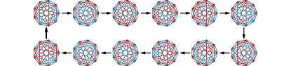
Figure 1: An example of a perfect limit cycle on a complete graph on $N=9$ nodes. The cycle consists of $c=12$ configurations. They are drawn in the order they appear in the cycle. Edges for $s_{ij}=1$ are in red and for $s_{ij}=-1$ in blue. Labels of vertices are not displayed. Vertices are numbered $i=1,\ldots,9$ clockwise, starting from the vertex $1$ on the top. The configuration in the left upper corner is equivalent to that given by the matrix (9).

Also the number of triangles by which $A_{t}$ and $A_{t+s}$ differ is constant for all $t$ when $s$ is fixed, and it is $D_{H}(A_{t},A_{t+s})=36,32,16,32,36,0$ for $s=1,2,3,4,5,6$.

Let us also mention some other features that are present for all such cycles. There are six types of edges which differ in the sequence of states: (1) three links remain constant ($+1$ or $-1$) with energy $E_{ij}=-s_{ij}\sum_{k}s_{ik}s_{kj}$ equal to -7; (2) four links change $12$ times, with $E_{ij}=+1$; (3) six links change $4$ times ($s_{ij}=1,1,1,-1,-1,-1$ and cyclically, $E_{ij}=-1,-5,+1$ and cyclically); (4) three links change $8$ times ($s_{ij}=-1,-1,+1$ and cyclically, $E_{ij}=-1,+3,+3$ and cyclically); (5) eight links change $6$ times ($s_{ij}=1,1,-1,-1$ and cyclically, $E_{ij}=-1,+1$ and cyclically); (6) twelve links change $6$ times ($s_{ij}=-1,-1,1,1,-1,1,1,1,-1,-1,1,-1$, $E_{ij}=-1,+5,-3,+1,+3,-3$ and cyclically.

Positions of states in the cycle are in equivalent in the sense that measuring relative changes to other states in the cycle you are not able to distinguish the states. This equivalence must be rooted in a symmetry of the system. There are two basic symmetries that should be taken into account: the automorphism of the complete graph, that is equivalent to the permutation of indices of the complete graph, and the gauge symmetry of spin configurations which preserves triangle energies. The hypothesis is that every configuration of a perfect cycle can be obtained from the previous one by a permutation of indices and a gauge transformation of spins. This in turn means that there exists a permutation of indices $\pi$ of indices such that $A_{t+1}\asymp\pi(A_{t})$. We have tested this hypothesis for $N=9$. Applying the update rule to the state (9), that we denote by $A_{t}$, we obtained a state $A_{t+1}$. Then we have determined all permutations $\pi$’s such that $A_{t+1}\asymp\pi(A_{t})$ by checking if the condition

$$D_{H}(A_{t+1},\pi(A_{t}))=0$$ (10)

is fulfilled.We have found that there are eight such permutations:

$$\begin{split}\pi_{1}&=(7,3,2,4,9,1,6,8,5)\\ \pi_{2}&=(7,3,2,8,9,1,6,4,5)\\ \pi_{3}&=(7,3,9,4,2,1,6,8,5)\\ \pi_{4}&=(7,3,9,8,2,1,6,4,5)\\ \pi_{5}&=(7,5,2,4,9,1,6,8,3)\\ \pi_{6}&=(7,5,2,8,9,1,6,4,3)\\ \pi_{7}&=(7,5,9,4,2,1,6,8,3)\\ \pi_{8}&=(7,5,9,8,2,1,6,4,3)\end{split}.$$ (11)

Renaming $A_{t+1}$ to $A_{t}$ and applying equation (10) we have again found the same eight permutations. It turns out, that the same eight permutations map any configuration onto the next configurations in the cycle. The permutations can be determined by exhaustive search but such a procedure is inefficient because there are $9!$ permutations. One can improve the search using the information encoded in the node energy lists of the configurations of the cycle, see Table 2. By analysing migration of node energies in consecutive configurations of the cycle one can learn about the corresponding permutations of indices which fulfill the condition (10). For example, energy $10$ moves from the position $1$ to $7$, from $7$ to $6$ and from $6$ to $1$. This means that the permutation has a cycle $(7,6,1)$. This in turn reduces the number of remaining permutations to $6!$. Further, by analysing migration of remaining items row by row in Table 2, one can find other cycles and reconstruct all the permutations (11). For completeness we give the cycle decomposition of the permutations: $\pi_{1}=(7,6,1)(3,2)(9,5)$, $\pi_{2}=(7,6,1)(3,2)(8,4)(9,5)$, $\pi_{3}=(7,6,1)(3,9,5,2)$, $\pi_{4}=(7,6,1)(3,9,5,2)(8,4)$, $\pi_{5}=(7,6,1)(5,9,3,2)$, $\pi_{6}=(7,6,1)(5,9,3,2)(8,4)$, $\pi_{7}=(7,6,1)(5,2)(9,3)$ and $\pi_{8}=(7,6,1)(5,2)(9,3)(8,4)$. We can use the result to calculate the number of the corresponding cycles. Each cycle is represented by twelve tables like Table 2. Twelve tables which differ by a cyclic permutation of rows are equivalent, since for a cycle it does not matter which configuration is listed first. Any permutation of columns (nodes) produces a table with the same node energy spectrum but possible with different positions on the lists. The tables obtained by $9!$ permutations generically correspond to different cycles, but not always. One has to take into account that eight permutations (11) produce a cyclic shift of rows in the table, as follows from the fact that the effect of the these permutations is equivalent to applying one step the dynamics (1). Thus permutations of indices generate $9!/8/12$ non-equivalent tables. Due to the gauge symmetry, each energy configuration is realised by $2^{8}$ distinct spin configurations. Putting theses factors together, we find that there are

$$\frac{9!}{8\cdot 12}2^{8}=967680$$ (12)

distinct perfect cycles having the node energy spectrum $n_{n}(10)=1$, $n_{n}(-2)=5$, $n_{n}(-6)=3$. We have confirmed this prediction numerically by checking the effect of the action of the transformation (1) for all configurations for $N=9$. We also found that there are no other cycles of length $c=12$ for $N=9$.

	1	2	3	4	5	6	7	8	9
1	10	-2	-2	-6	-2	-6	-2	-6	-2
2	-6	-2	-2	-6	-2	-2	10	-6	-2
3	-2	-2	-2	-6	-2	10	-6	-6	-2
4	10	-2	-2	-6	-2	-6	-2	-6	-2
5	-6	-2	-2	-6	-2	-2	10	-6	-2
6	-2	-2	-2	-6	-2	10	-6	-6	-2
7	10	-2	-2	-6	-2	-6	-2	-6	-2
8	-6	-2	-2	-6	-2	-2	10	-6	-2
9	-2	-2	-2	-6	-2	10	-6	-6	-2
10	10	-2	-2	-6	-2	-6	-2	-6	-2
11	-6	-2	-2	-6	-2	-2	10	-6	-2
12	-2	-2	-2	-6	-2	10	-6	-6	-2

Table 2: Each row contains a list of node energies of a configuration of the cycle. The row in the table header numbers the nodes, and the column on the left side numbers the successive cycle configurations. The node energy spectrum is steady: $n_{n}(10)=1$, $n_{n}(-2)=5$ and $n_{n}(-6)=3$.

The perfect cycles of length $c=12$ for $N=9$ have relatively small basins of attraction which consist of $312$ states including the $12$ states belonging to the cycle and $300$ other states. $12$ out of $300$ states are mirror states of those belonging to the cycle. Mirror state $s^{*}$ of a state $s$ is a state with all opposite signs $s^{*}_{ij}=-s_{ij}$ for all $ij$. The remaining $288$ states can be divided into $12$ groups, each having $12$ pairs of mutually mirror states. Each of the $12$ groups is associated with one state of the cycle to which all $24$ states from the group are transformed in a single step of the dynamics (1). None of $300$ states has a predecessor. Such states are sometimes called ’Garden of Eden’ m .

We have also studied systems for $N>9$ to search for perfect cycles. In this case, however, we performed a random search since as mentioned the number of configurations is too large for these systems to be exhaustively browsed. We have found perfect cycles of length $c=14$ for $N=11$. The edge energy spectra of these cycles is shown in Table 3.

$u$	-9	-7	-5	-3	-1	+1	+3	+5	+7	+9
$n_{e}(u)$	0	0	4	10	15	13	9	3	1	0

Table 3: Edge energy spectrum of states belonging to the perfect cycle of length $c=14$ for $N=11$.

As follows from the table, energy of the configurations is $U=\frac{1}{3}\sum_{u}un_{e}(u)=-1$, and the Hamming distance between any two neighbouring states in the cycle (8) is $d_{H}(A_{t},A_{t+1})=\sum_{u>0}n_{e}(u)=26$. The corresponding node energy spectrum is $n_{n}(-9)=1$, $n_{n}(-5)=4$, $n_{n}(3)=4$, $n_{n}(7)=2$ and $n_{n}(u)=0$ for other values of $u$. As before we found that $d_{H}(A_{t},A_{t+s})$ and $D_{H}(A_{t},A_{t+s})$ for fixed $s$ are independent of $t$, so all configurations of the cycle are equivalent, and symmetrically distributed in the configuration space. We found that there are two distinct permutations fulfilling the condition (10). They can be decomposed into a cycle of length seven and two cycles of length two. Using the same enumeration argument as before (12) this gives $11!/2/14\times 2^{10}$ such cycles. One would need to check all configurations, to exclude that there are no other cycles (with a different energy spectrum) for $N=11$. We have also found a perfect cycle of length $c=12$ for $N=13$. The edge energy spectrum is given in Table 4. The energy of the configurations is $U=\frac{1}{3}\sum_{u}un_{e}(u)=-56$, and the Hamming distance between any two neighbouring states in the cycle (8) is $d_{H}(A_{t},A_{t+1})=\sum_{u>0}n_{e}(u)=20$.

$u$	-11	-9	-7	-5	-3	-1	+1	+3	+5	+7	+9	+11
$n_{e}(u)$	1	3	7	8	21	18	12	6	2	0	0	0

Table 4: Edge energy spectrum of states belonging to the perfect cycle of length $c=12$ for $N=13$.

The node energy spectrum is $n_{n}(-20)=4$, $n_{n}(-16)=2$, $n_{n}(-12)=4$, $n_{n}(-4)=-2$, $n_{n}(0)=1$. Again we found that $d_{H}(t,t+s)$ and $D_{H}(t,t+s)$ are independent on $t$ when $s$ is constant.

IV Semi-perfect cycles

Not all limit cycles have steady energy spectra. There are cycles whose spectra change periodically. We will call them semi-perfect. As an example let us discuss a semi-perfect cycle that we have found for $N=13$. The cycle is representative for all semi-perfect cycles in that that it has typical features, but additionally it is the longest limit cycle we have found so far. It has the length of $c=48$. The energy spectra of the states in the cycle change with the period three. The edge spectra of three consecutive states of the cycle are given in Table 5.

$u$	-11	-9	-7	-5	-3	-1	+1	+3	+5	+7	+9	+11
$n_{e}(u)$	2	0	3	11	17	15	17	8	4	1	0	0
$n_{e}(u)$	2	2	6	8	10	16	16	17	1	0	0	0
$n_{e}(u)$	2	0	2	9	18	15	20	9	2	0	1	0

Table 5: Edge energy spectra of three consecutive states belonging to the semi-perfect cycle of length $c=48$ for $N=13$.

Energies of the states are $U_{t}=-32,-32,-28$. The Hamming distance between neighbouring states is $d_{H}(t,t+1)=34,32,30$ and $D_{H}(t,t+1)=128,136,134$. The values repeat every three steps. If we denote the map corresponding to a single state (1) by $s(t+1)=\Phi(s(t))$, then taking every third configuration is equivalent to $s(t+3)=\Phi(\Phi(\Phi(s(t))))=\Psi(s(t))$ where the map is a triple composition of $\Phi$: $\Psi=\Phi\circ\Phi\circ\Phi$. Viewed from this perspective, the semi-perfect cycle of the dynamics defined by the map $\Phi$ (1) is a perfect cycle for $\Psi$. More generally, the class of semi-perfect cycles is a class of limit cycles which are perfect for a multiple composition $\Phi\circ\ldots\circ\Phi$ of the original update rule.

V Discussion

The motivation behind the evolution rule (1) is that it locally maximises the number of balanced triads. Indeed, when performed asynchronously, that is one edge at time, the rule never reduces the number of balanced triads and thus it leads to a state at local maximum, as far as the number of balanced triads is concerned (equivalent to local energy minimum (2)). The synchronous version of the evolution (1) where all edges are updated simultaneously has a far more interesting spectrum of attractors: in addition to fixed points it has limit cycles of different length and of different symmetry. Some limit cycles are surprisingly long. For example we found a limit cycle of length $c=48$ for $N=13$. In this paper we mostly focused on a class of limit cycles which preserve the energy spectrum and are represented by symmetric trajectories in the configuration space, such that any two states separated by the same number of steps in the perfect cycle are separated by the same Hamming distance in the configuration space. We have argued that the symmetry of these trajectories is rooted in the automorphism group of the complete graph on which the system is defined and in the local gauge symmetry of the energy function (2).

There are many open questions. Is it possible to formulate general conditions that would make it possible to judge whether a state belongs to a limit cycle, before checking it explicitly by iterating the equation (1)? What is the longest limit cycle and the longest perfect cycle for the complete network for given $N$? What is the abundance of such cycles? We know kkb that the fraction of initial states which lead to perfect limit cycles of length $c=14$ for $N=11$ is about $10^{-6}$, which is much less than the fraction of perfect cycles $c=12$ for $N=9$ which is $0.004$. We expect that the percentage of states of perfect cycles decreases with the system size, but it would be good to find an argument about asymptotic behaviour.

Generally, the dynamics we discussed in this paper is of the type $s(t+1)=\Phi(s(t))$. The map $\Phi$ given by Eq. (1) is just a particular case. One can change the evolution rule. For example adding a minus sign to the expression on the right hand side of Eq. (1) we would obtain a system having a tendency to maximize the number of frustrated triads. Of course this evolution would be in one-to-one correspondence to the one discussed here as can be seen by replacing states $s$ in one original dynamics by mirror states $s^{*}$ in the new one. But the question about how the attractors of the evolution depend on the given map $\Phi$ is quite interesting. For example what is the class of maps $\Phi$ which would lead to perfect limit cycles? It would be interesting to study symmetry classes for general maps k2 .

There is some correspondence of the dynamics of the model discussed in this paper and the quenched Kauffman NK model k1 ; ack of time evolution of networks. As we argued in kkb , here the number K of incoming links which determine the current state of a node (here: of a link) evolves with the number of degrees of freedom (here: $N^{2}$) as a square root of this number (here $N$). An important difference is that in our case, there is only one function (given by Eq. (1)) which determines the state of each link in a subsequent time, and not a random (fixed in the quenched model) set of these functions, different for each node. What is similar is the large number of steady states with minimal energy, which in our case is just the number of balanced states, varying with $N$ as $2^{N-1}$. We add that the process of reaching the Heider balance, modeled by Eq. (1), has been termed as ’social mitosis’ wt . Limit cycles in the Kauffman model bp ; bs are no less important than fixed points and have biological interpretation. Our results indicate that limit cycles can also occur when evolution is deterministic and identical for all components of the system.

References

- (1) M. J. Krawczyk, K. Kułakowski and Z. Burda, Towards the Heider balance: Cellular automaton with a global neighborhood, Phys. Rev. E 104 (2021) 024307.
- (2) F. Heider, Attitudes and cognitive organization, J. of Psychology 21 (1) (1946) 107-112.
- (3) T. Antal, P. L. Krapivsky and S. Redner, Dynamics of social balance on networks, Phys. Rev. E 72 (2005) 036121.
- (4) K. Kułakowski, P. Gawroński and P. Gronek, The Heider balance: A continuous approach, Int. J. Mod. Phys. C 16 (5) (2005) 707-716.
- (5) T. Antal, P. Krapivsky and S. Redner, Social balance on networks: The dynamics of friendship and enmity, Physica D: 224 (1) (2006) 130-136.
- (6) S. A. Marvel, J. Kleinberg, R. D. Kleinberg and S. H. Strogatz, Continuous-time model of structural balance, PNAS 108 (5) (2011) 1771-1776.
- (7) K. Malarz, M. Wołoszyn and K. Kułakowski, Towards the Heider balance with a cellular automaton, Physica D 411 (2020) 132506.
- (8) E. F. Moore, Machines models of self-reproduction, Proc. Symp. Appl. Math. 14 (1962) 17.
- (9) M. J. Krawczyk, Symmetry induced compression of discrete phase space, Physica A 390 (2011) 2181.
- (10) S. A. Kauffman, The Origins of Order: Self-Organization and Selection in Evolution, Oxford University Press, New York 1993.
- (11) M. Aldana, S. Coppersmith and L. P. Kadanoff, Boolean dynamics with random coupling, Perspectives and Problems in Nonlinear Science, 2003, pp 23 - 89.
- (12) Z. Wang and W. Thorngate, Sentiment and social mitosis: Implications of Heider’s balance theory, JASSS 2003, vol 6.
- (13) U. Bastolla and G. Parisi, A numerical study of the critical line of Kauffman networks, J. of Theor. Biol. 187 (1997) 117-133.
- (14) S. Bilke and F. Sjunnesson, Stability of the Kauffman model, Phys. Rev. E 65 (2002) 016129.