Solving Nonconvex-Nonconcave Min-Max Problems exhibiting Weak Minty Solutions

Axel BΓΆhm Faculty of Mathematics, University of Vienna, Oskar-Morgenstern-Platz 1, 1090 Vienna, Austria. Research supported by the doctoral programme Vienna Graduate School on Computational Optimization (VGSCO), FWF (Austrian Science Fund), project W 1260. axel.boehm@univie.ac.at
Abstract

We investigate a structured class of nonconvex-nonconcave min-max problems exhibiting so-called weak Minty solutions, a notion which was only recently introduced and already prooved powerful by simultaneously capturing different generalizations of monotonicity. We prove novel convergence results for a generalized version of the optimistic gradient method (OGDA) in this setting, matching the 1/k1π‘˜1/k rate for the best iterate in terms of the squared operator norm recently shown for the extragradient method (EG). In addition we propose an adaptive step size version of EG, which does not require knowledge of the problem parameters.

1 Introduction

The recent success of machine learning models which can be described by min-max optimization, such as generative adversarial networksΒ [21], adversarial learningΒ [36], adversarial example gamesΒ [6] or actor-critic methodsΒ [45], has sparked interest in such saddle point problems. While methods have been identified, which (mostly) work in practice, the setting in which the objective function is nonconvex in the minimization and nonconcave in the maximization component remains theoretically poorly understood and even shows intractability resultsΒ [17, 30]. Recently,Β [14] studied a class of nonconvex-nonconcave min-max problems and observed that the extragradient method (EG) showed good converge behavior in the experiments. Surprisingly, the problems did not seem to exhibit any of the known tame properties such as monotonicity, or Minty solutions. Later,Β [18] found the appropriate notion (see AssumptionΒ 1), which is weaker than the existence of a Minty solution (an assumption extensively used in the literatureΒ [38, 34, 35]) and also generalizes the concept of negative comonotonicityΒ [4, 11, 30]. Due to these unifying and generalizing properties the notion of weak Minty solutions was promptly studied inΒ [44, 31].

Assumption 1 (Weak Minty solution).

Given an operator F:ℝd→ℝd:𝐹→superscriptℝ𝑑superscriptℝ𝑑F:\mathbb{R}^{d}\to\mathbb{R}^{d} there exists a point uβˆ—βˆˆβ„dsuperscript𝑒superscriptℝ𝑑u^{*}\in\mathbb{R}^{d} and a parameter ρ>0𝜌0\rho>0 such that

⟨F​(u),uβˆ’uβˆ—βŸ©β‰₯βˆ’Ο2​‖F​(u)β€–2βˆ€uβˆˆβ„d.formulae-sequence𝐹𝑒𝑒superscriptπ‘’πœŒ2superscriptnorm𝐹𝑒2for-all𝑒superscriptℝ𝑑\langle F(u),u-u^{*}\rangle\geq-\frac{\rho}{2}\|F(u)\|^{2}\quad\forall u\in\mathbb{R}^{d}. (1)

Additionally,Β [18] proved that a generalization of EGΒ [29] is able to solve problems which exhibit such solutions with a complexity of π’ͺ​(Ξ΅βˆ’1)π’ͺsuperscriptπœ€1\mathcal{O}(\varepsilon^{-1}) for the squared operator norm. This modification which they title EG++, is based on an aggressive extrapolation step combined with a conservative update step. Such a step size policy has already been explored in the context of a stochastic version of EG inΒ [27].

In a similar spirit we investigate a variant of the optimistic gradient descent ascent (OGDA)Β [15, 46]/Forward-Reflected-Backward (FoRB)Β [39] method. We pose the question, and give an affirmative answer to:

Can OGDA match the convergence guarantees of EG in the presence of weak Minty solutions?

In particular, we show that the following modification of the OGDA method, given for step size a>0π‘Ž0a>0 and parameter 0<γ≀10𝛾10<\gamma\leq 1 by

uk+1=ukβˆ’a​((1+Ξ³)​F​(uk)βˆ’F​(ukβˆ’1)),βˆ€kβ‰₯0,formulae-sequencesubscriptπ‘’π‘˜1subscriptπ‘’π‘˜π‘Ž1𝛾𝐹subscriptπ‘’π‘˜πΉsubscriptπ‘’π‘˜1for-allπ‘˜0u_{k+1}=u_{k}-a\Bigl{(}(1+\gamma)F(u_{k})-F(u_{k-1})\Bigr{)},\quad\forall k\geq 0,

is able to match the bounds of EG++Β [18, 44]:

uk=uΒ―kβˆ’a​F​(uΒ―k),uΒ―k+1=uΒ―kβˆ’Ξ³β€‹a​F​(uk),βˆ€kβ‰₯0,formulae-sequencesubscriptπ‘’π‘˜subscriptΒ―π‘’π‘˜π‘ŽπΉsubscriptΒ―π‘’π‘˜formulae-sequencesubscriptΒ―π‘’π‘˜1subscriptΒ―π‘’π‘˜π›Ύπ‘ŽπΉsubscriptπ‘’π‘˜for-allπ‘˜0u_{k}=\bar{u}_{k}-aF(\bar{u}_{k}),\quad\bar{u}_{k+1}=\bar{u}_{k}-\gamma aF(u_{k}),\quad\forall k\geq 0,

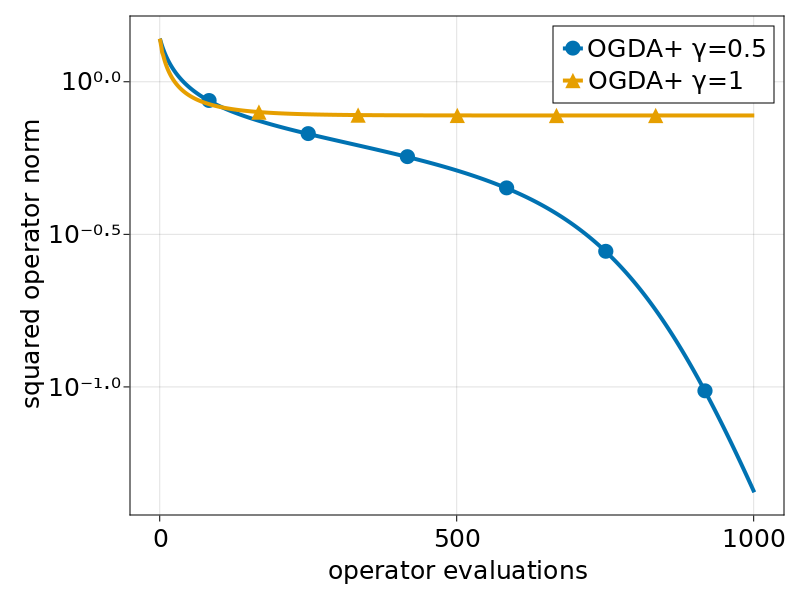
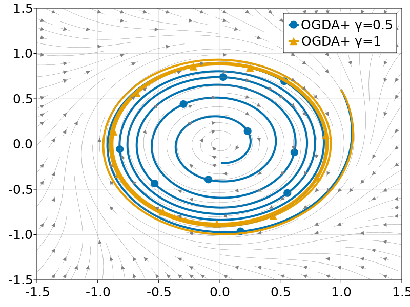
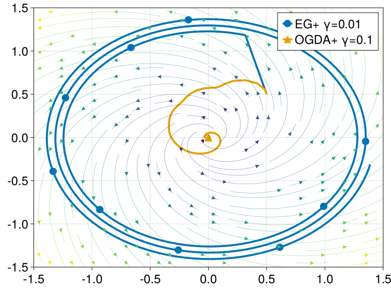
by only requiring one gradient oracle call per iteration. In FigureΒ 1 we see that beyond the theoretical guarantees OGDA++ can even provide convergence where EG++ does not.

Note that OGDA is most commonly written in the form where Ξ³=1𝛾1\gamma=1, seeΒ [15, 39, 5], with the exception of two recent works which have investigated a more general coefficient seeΒ [49, 41]. While the previous references target the monotone setting the true importance of γ𝛾\gamma only shows up in the presence of weak Minty solutions as in this case we require it to be larger than 111 to guarantee convergence β€” a phenomenon not present for monotone problems.

Connection to min-max.

When considering a general (smooth) min-max problem

minx⁑maxy⁑f​(x,y)subscriptπ‘₯subscript𝑦𝑓π‘₯𝑦\min_{x}\max_{y}\,f(x,y)

the operator F𝐹F mentioned in AssumptionΒ 1 arises naturally as F​(u):=[βˆ‡xf​(x,y),βˆ’βˆ‡yf​(x,y)]assign𝐹𝑒subscriptβˆ‡π‘₯𝑓π‘₯𝑦subscriptβˆ‡π‘¦π‘“π‘₯𝑦F(u):={[\nabla_{x}f(x,y),-\nabla_{y}f(x,y)]} with u=(x,y)𝑒π‘₯𝑦u=(x,y). However, by studying saddle point problems from this more general perspective of variational inequalities (VIs), seeΒ (SVI), via the operator F𝐹F we can simultaneously capture more settings such as certain equilibrium problems, seeΒ [19].

About the weak Minty parameter ρ𝜌\rho.

The parameter ρ𝜌\rho in the definition of weak Minty solutionsΒ (1) plays a crucial role in the analysis and the experiments. In particular it is necessary that the step size is larger than a term proportional to ρ𝜌\rho, see for example TheoremΒ 3.1 orΒ [44]. At the same time, as typical, the step size is constrained from above by the reciprocal of the Lipschitz constant of F𝐹F. For example, since the authors ofΒ [18] require the step size to be less than 1L1𝐿\frac{1}{L}, their convergence statement only holds if ρ<14​L𝜌14𝐿\rho<\frac{1}{4L} for the choice Ξ³=12𝛾12\gamma=\frac{1}{2}. This was later improved inΒ [44] to 1L1𝐿\frac{1}{L} for γ𝛾\gamma even smaller. As in the monotone setting, OGDA however, requires a smaller step size than EG.Β Nevertheless, through a different analysis we are able to match the most general condition on the weak Minty parameter ρ<1L𝜌1𝐿\rho<\frac{1}{L} for appropriate γ𝛾\gamma and aπ‘Ža.

Contribution.
  1. 1.

    Building on the recently introduced notion of weak solutions to the Minty variational inequality, seeΒ [18], we prove a novel convergence rate of π’ͺ​(1/k)π’ͺ1π‘˜\mathcal{O}(1/k) in terms of the squared operator norm for a modification of OGDA, which we name OGDA++, matching the one of EG.

  2. 2.

    Even under the stronger assumption that the operator is moreover monotone we improve the possible range of step sizes for OGDA++Β [49] and recover the best known result for the standard method (Ξ³=1𝛾1\gamma=1)Β [23].

  3. 3.

    We prove a complexity bound of π’ͺ​(Ξ΅βˆ’2)π’ͺsuperscriptπœ€2\mathcal{O}(\varepsilon^{-2}) for a stochastic version of the OGDA++ method.

  4. 4.

    Additionally, we propose an adaptive step size version of EG++, which is able to obtain the same convergence guarantees without any knowledge of the Lipschitz constant of the operator F𝐹F, and therefore possibly even take larger steps in regions of low curvature and allow for convergence where a fixed step size policy does not.
Refer to caption
(a) Performance of methods.
Refer to caption
(b) Trajectories of iterates.
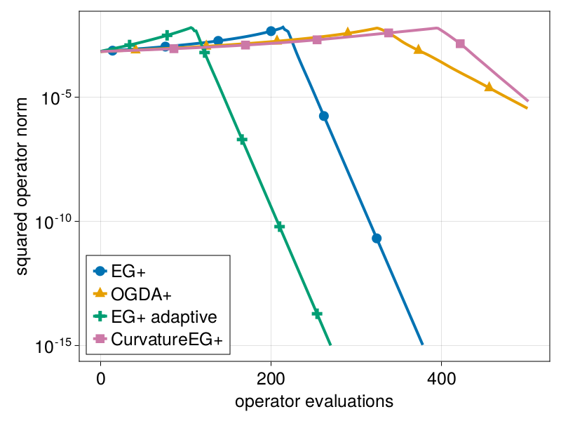
Figure 1: Problem (7), with ρ=1L𝜌1𝐿\rho=\frac{1}{L}, meaning that convergence is not covered by theory. Since the Lipschitz constant can be computed analytically we choose the step size accordingly. Due to the linearity of the operator F𝐹F there is no benefit in using linesearch, so only methods using constant step sizes are compared. Only OGDA++ converges.

1.1 Related literature

Since there is an extensive literature on convergence rates in terms of a gap function or distance to a solution for monotone problems as well as generalizations such as nonconvex-concave [7, 33], convex-nonconcave [52] or under the Polyak-Łojasiewicz assumption, see [54], we will only focus on the nonconvex-nonconcave setting.

Weak minty.

[18] noticed that a particular parametrization of the von Neumann ratio game exhibits a new type of solution, which they titled weak Minty, without possessing any of the known properties such as (negative) comonotonicity or Minty solutions. They showed convergence in the presence of such solutions for EG if the extrapolation step size is twice as large as the update step. LaterΒ [44] showed that the condition on the weak Minty parameter can be relaxed by reducing the length of the update step even further and they do so in an adaptive way. In order to not require any other hyperparameters they also propose a backtracking line search, which might come at the cost of additional gradient computations or the use of second order information (in contrast to the adaptive step size we propose in AlgorithmΒ 3). InΒ [31] a different approach is taken by restricting the attention to the min-max setting and using multiple ascent steps per descent step, obtaining the same π’ͺ​(1/k)π’ͺ1π‘˜\mathcal{O}(1/k) rate as EG.

Minty solutions.

Many works have shown different approaches for when the problem at hand exhibits a Minty solution, seeΒ (MVI). The authors ofΒ [35] showed that weakly monotone VIs can be solved by successively adding a quadratic proximity term and repeatedly optimizing the resulting strongly monotone VI with any convergent method. InΒ [40] the convergence of the OGDA method was proven, but without any rate. InΒ [38] it was noted that the convergence proof for the golden ratio algorithm (GRAAL) works without any modification. See alsoΒ [13] for a non-euclidean version of EG andΒ [34] for adaptive methods. While the assumption that a Minty solution exists is a generalization of the monotone setting it is difficult to find nonmonotone problems that do possess such solutions. In our setting, see AssumptionΒ 1, the Minty inequalityΒ (MVI) is allowed to be violated at every point by a factor proportional to the squared operator norm.

Negative comonotonicity.

While previously studied under the name of cohypomonotonicityΒ [11] the notion of negative comonotonicity was recently explored inΒ [4]. It provides a generalization of monotonicity, but in a direction different from the notion of Minty solutions and only a few works have analyzed methods in this setting. The authors ofΒ [30] studied an anchored version of EG and showed an improved convergence rate of π’ͺ​(1/k2)π’ͺ1superscriptπ‘˜2\mathcal{O}(1/k^{2}) (in terms of the squared operator norm). Similarly,Β [9] studied an accelerated version of the reflected gradient method [37]. It is an open question whether such an acceleration is possible in the more general setting of weak Minty solutions (any Stampacchia solution to the VI given by negatively comonotone operator is a weak Minty solution). Another interesting observation was made inΒ [24] where for cohypomonotone problems monotonically decreasing gradient norm was shown when using EG.Β However, we did not observe this in our experiments, highlighting the need to distinguish this class from problems with weak Minty solutions.

Interaction dominance.

The authors ofΒ [25] investigate the notion of α𝛼\alpha-interaction dominance for nonconvex-nonconcave min-max problems and showed that the proximal-point method converges sublinearly if this condition holds in y𝑦y and linearly if it holds in both components. FurthermoreΒ [30] showed that if a problem is interaction dominant in both components, then it is also negatively comonotone.

Optimism.

The beneficial effects of introducing the simple modification commonly known as optimism have recently sparked the interest of the machine learning communityΒ [15, 16, 32, 20]. Its name originates from online optimizationΒ [47, 48]. The idea dates back even furtherΒ [46] and has been studied in the mathematical programming community as wellΒ [37, 39, 12].

2 Preliminaries

2.1 Notions of solution

We summarize the most commonly used notions of solutions appearing in the context of variational inequalities (VIs) and beyond. Note that these are commonly defined in terms of a constraint set CβŠ‚β„d𝐢superscriptℝ𝑑C\subset\mathbb{R}^{d}. A Stampacchia111Sometimes Stampacchia and Minty solutions are referred to as strong and weak solutions respectively, seeΒ [42], but we will refrain from this nomenclature, as it is confusing in the context of weak Minty solutions.Β [28] solution of the VI given by F:ℝd→ℝd:𝐹→superscriptℝ𝑑superscriptℝ𝑑F:\mathbb{R}^{d}\to\mathbb{R}^{d} is defined as a point uβˆ—superscript𝑒u^{*} such that

⟨F​(uβˆ—),uβˆ’uβˆ—βŸ©β‰₯0βˆ€u∈C.formulae-sequence𝐹superscript𝑒𝑒superscript𝑒0for-all𝑒𝐢\langle F(u^{*}),u-u^{*}\rangle\geq 0\quad\forall u\in C. (SVI)

In particular we only consider in this manuscript the unconstrained case C=ℝd𝐢superscriptℝ𝑑C=\mathbb{R}^{d} in which case the above condition reduces to F​(uβˆ—)=0𝐹superscript𝑒0F(u^{*})=0. Very much related with a long tradition is the following. A Minty11footnotemark: 1 solution is given by a point uβˆ—βˆˆCsuperscript𝑒𝐢u^{*}\in C such that

⟨F​(u),uβˆ’uβˆ—βŸ©β‰₯0βˆ€u∈C.formulae-sequence𝐹𝑒𝑒superscript𝑒0for-all𝑒𝐢\langle F(u),u-u^{*}\rangle\geq 0\quad\forall u\in C. (MVI)

If F𝐹F is continuous, a Minty solution of the VI is always a Stampacchia solution. The reverse is in general not true but holds for example if the operator F𝐹F is monotone. In particular, there exist nonmonotone problems with Stampacchia solutions but without any Minty solutions.

2.2 Notions of monotonicity

The aim of this section is to recall some elementary and some more recent notions of monotonicity and the connection between those. We call an operator F𝐹F monotone if

⟨F​(u)βˆ’F​(v),uβˆ’v⟩β‰₯0.𝐹𝑒𝐹𝑣𝑒𝑣0\langle F(u)-F(v),u-v\rangle\geq 0.

Such operators arise naturally as the gradients of convex functions, from convex-concave min-max problems or from equilibrium problems.

Two notions frequently studied that fall in this class are strongly monotone operators fulfilling

⟨F​(u)βˆ’F​(v),uβˆ’v⟩β‰₯μ​‖uβˆ’vβ€–2.πΉπ‘’πΉπ‘£π‘’π‘£πœ‡superscriptnorm𝑒𝑣2\langle F(u)-F(v),u-v\rangle\geq\mu\|u-v\|^{2}.

They appear as gradients of strongly convex functions or strongly-convex-strongly-concave min-max problems. A second subclass of monotone operators are so-called cocoercive operators fulfilling

⟨F​(u)βˆ’F​(v),uβˆ’v⟩β‰₯β​‖F​(u)βˆ’F​(v)β€–2.𝐹𝑒𝐹𝑣𝑒𝑣𝛽superscriptnorm𝐹𝑒𝐹𝑣2\langle F(u)-F(v),u-v\rangle\geq\beta\|F(u)-F(v)\|^{2}. (2)

They appear, for example, as gradients of smooth convex functions, in which case 2 holds with β𝛽\beta equal to the reciprocal of the gradients Lipschitz constant.

Leaving the monotone world.

Both subclasses of monotonicity introduced above can be used as starting points to venture into the non-monotone world. Since general non-monotone operators might exhibit erratic behavior like periodic cycles and spurious attractors [26], it makes sense to find settings that extend the monotone one, but still remain tractable. First and foremost, the by now well-studied setting of ν𝜈\nu-weak monotonicity

⟨F​(u)βˆ’F​(v),uβˆ’v⟩β‰₯βˆ’Ξ½β€‹β€–uβˆ’vβ€–2.πΉπ‘’πΉπ‘£π‘’π‘£πœˆsuperscriptnorm𝑒𝑣2\langle F(u)-F(v),u-v\rangle\geq-\nu\|u-v\|^{2}.

Such operators arise as the gradients of the well-studied class (seeΒ [dima_damek_stoch_weakly_k-4]) of weakly convex functions β€” a rather generic class of functions as it includes all functions without upward cusps. In particular every smooth function with Lipschitz gradient turns out to fulfill this property. On the other hand, extending the notion of cocoercivity to allow for negative coefficients, referred to as cohypomonotonicity, has received much less attentionΒ [4, 11] and is given by

⟨F​(u)βˆ’F​(v),uβˆ’v⟩β‰₯βˆ’Ξ³β€‹β€–F​(u)βˆ’F​(v)β€–2.𝐹𝑒𝐹𝑣𝑒𝑣𝛾superscriptnorm𝐹𝑒𝐹𝑣2\langle F(u)-F(v),u-v\rangle\geq-\gamma\|F(u)-F(v)\|^{2}.

Clearly, if there exists a Stampacchia solution for such an operator, then it also fulfills AssumptionΒ 1.

Behavior w.r.t.Β the solution.

While the above properties are standard assumption in the literature, it is usually sufficient to ask for the corresponding condition to hold when one of the arguments is a (Stampacchia) solution. This means instead of monotonicity it is enough to obtain standard convergence results, see [22], to ask for the operator F𝐹F to be star-monotone [43], i.e.

⟨F​(u),uβˆ’uβˆ—βŸ©β‰₯0𝐹𝑒𝑒superscript𝑒0\langle F(u),u-u^{*}\rangle\geq 0

or star-cocoerciveΒ [22]

⟨F​(u),uβˆ’uβˆ—βŸ©β‰₯γ​‖F​(u)β€–2.𝐹𝑒𝑒superscript𝑒𝛾superscriptnorm𝐹𝑒2\langle F(u),u-u^{*}\rangle\geq\gamma\|F(u)\|^{2}.

In this spirit, we can provide a new interpretation to the assumption of the existence of a weak Minty solution as asking for the operator F𝐹F to be negatively star-cocoercive (with respect to at least one solution). Furthermore, we want to point out that while the above star notions are sometimes required to hold for all solutions uβˆ—superscript𝑒u^{*}, in the following we only require it to hold for a single solution.

3 OGDA for problems with weak Minty solutions

The generalized version of OGDA, whose name we equip in the spirit ofΒ [18, 44], with a β€œ++” to highlight the presence of the additional parameter γ𝛾\gamma, is given by:

Algorithm 1 OGDA++

Require: Starting point u0=uβˆ’1βˆˆβ„dsubscript𝑒0subscript𝑒1superscriptℝ𝑑u_{0}=u_{-1}\in\mathbb{R}^{d}, step size a>0π‘Ž0a>0 and parameter 0<γ≀10𝛾10<\gamma\leq 1.

forΒ k=0,1,β€¦π‘˜01…k=0,1,\dotsΒ do
Β Β Β Β Β uk+1=ukβˆ’a​((1+Ξ³)​F​(uk)βˆ’F​(ukβˆ’1))subscriptπ‘’π‘˜1subscriptπ‘’π‘˜π‘Ž1𝛾𝐹subscriptπ‘’π‘˜πΉsubscriptπ‘’π‘˜1u_{k+1}=u_{k}-a\Big{(}\left(1+\gamma\right)F(u_{k})-F(u_{k-1})\Big{)}
Theorem 3.1.

Let F:ℝd→ℝd:𝐹→superscriptℝ𝑑superscriptℝ𝑑F:\mathbb{R}^{d}\to\mathbb{R}^{d} be L𝐿L-Lipschitz continuous satisfying AssumptionΒ 1 with 1L>ρ1𝐿𝜌\frac{1}{L}>\rho and (uk)kβ‰₯0subscriptsubscriptπ‘’π‘˜π‘˜0{(u_{k})}_{k\geq 0} be the iterates generated by AlgorithmΒ 1 with step size aπ‘Ža satisfying a>Οπ‘ŽπœŒa>\rho and

a​L≀1βˆ’Ξ³1+Ξ³.π‘ŽπΏ1𝛾1𝛾aL\leq\frac{1-\gamma}{1+\gamma}. (3)

Then, for all kβ‰₯0π‘˜0k\geq 0

mini=0,…,kβˆ’1⁑‖F​(ui)β€–2≀1k​a​γ​(aβˆ’Ο)​‖u0+a​F​(u0)βˆ’uβˆ—β€–2.subscript𝑖0β€¦π‘˜1superscriptnorm𝐹subscript𝑒𝑖21π‘˜π‘Žπ›Ύπ‘ŽπœŒsuperscriptnormsubscript𝑒0π‘ŽπΉsubscript𝑒0superscript𝑒2\min_{i=0,\dots,k-1}\|F(u_{i})\|^{2}\leq\frac{1}{ka\gamma(a-\rho)}\|u_{0}+aF(u_{0})-u^{*}\|^{2}.

In particular as long as ρ<1L𝜌1𝐿\rho<\frac{1}{L} we can find a γ𝛾\gamma small enough such that the above bound holds.

The first observation is that we would like to choose aπ‘Ža as large as possible as this allows us to treat the largest class of problems with ρ<aπœŒπ‘Ž\rho<a. In order to be able to choose the step size aπ‘Ža large we have to decrease γ𝛾\gamma as evident from 3. This, however degrades the speed of the algorithm as it makes the update steps smaller β€” the same effect can be observedΒ [44] for EG++ and is therefore not surprising. One could derive an optimal γ𝛾\gamma (i.e.Β minimizing the right hand side) from TheoremΒ 3.1, which however results in a uninsightful cubic dependence on ρ𝜌\rho. In practice, the strategy of decreasing γ𝛾\gamma until we get convergence, but not further gives reasonable results.

Furthermore, we want to point out that the condition ρ<1L𝜌1𝐿\rho<\frac{1}{L}, is precisely the best possible bound for EG++ in [44].

Refer to caption
(a) Performance of methods.
Refer to caption
(b) Trajectories of iterates.
Figure 2: Polar game fromΒ [44] with 18​L>ρ>110​L18𝐿𝜌110𝐿\frac{1}{8L}>\rho>\frac{1}{10L}. Shows the need to reduce γ𝛾\gamma in OGDA++.

3.1 Improved bounds under monotonicity

While the above theorem also holds if the operator F𝐹F is monotone, we can modify the proof slightly to obtain a better dependence on the parameters:

Theorem 3.2.

Let F:ℝd→ℝd:𝐹→superscriptℝ𝑑superscriptℝ𝑑F:\mathbb{R}^{d}\to\mathbb{R}^{d} be monotone and L𝐿L-Lipschitz. If a​L=2βˆ’Ξ³2+Ξ³βˆ’Ξ΅π‘ŽπΏ2𝛾2π›Ύπœ€aL=\frac{2-\gamma}{2+\gamma}-\varepsilon for Ξ΅>0πœ€0\varepsilon>0 then, the iterates generated by OGDA++ fulfill

mini=0,…,kβˆ’1⁑‖F​(ui)β€–2≀2k​a2​γ2​Ρ​‖u0+a​F​(u0)βˆ’uβˆ—β€–2.subscript𝑖0β€¦π‘˜1superscriptnorm𝐹subscript𝑒𝑖22π‘˜superscriptπ‘Ž2superscript𝛾2πœ€superscriptnormsubscript𝑒0π‘ŽπΉsubscript𝑒0superscript𝑒2\min_{i=0,\dots,k-1}\|F(u_{i})\|^{2}\leq\frac{2}{ka^{2}\gamma^{2}\varepsilon}\|u_{0}+aF(u_{0})-u^{*}\|^{2}.

In particular, we can choose Ξ³=1𝛾1\gamma=1 and a<13​Lπ‘Ž13𝐿a<\frac{1}{3L}.

There are different works discussing the convergence of OGDA in terms of the iterates or a gap function with a<12​Lπ‘Ž12𝐿a<\frac{1}{2L}, see for exampleΒ [39]. We, however, want to compare the above bound to more similar results on rates for the best iterate in terms of the operator norm. The same rate as ours for OGDA is shown inΒ [10] but requires the conservative step size bound a≀116​Lπ‘Ž116𝐿a\leq\frac{1}{16L}. This was later improved to a≀13​Lπ‘Ž13𝐿a\leq\frac{1}{3L} inΒ [23] where the bound even holds for the last iterate. However, all of these only deal with the case Ξ³=1𝛾1\gamma=1. The only other reference that deals with a generalized (i.e.Β not necessarily Ξ³=1𝛾1\gamma=1) version of OGDA isΒ [49]. There the resulting step size condition is a≀2βˆ’Ξ³4​Lπ‘Ž2𝛾4𝐿a\leq\frac{2-\gamma}{4L}, which is strictly worse than ours for any γ𝛾\gamma. To summarize, not only do we show for the first time that the step size of a generalization of OGDA can go above 12​L12𝐿\frac{1}{2L} we also provide the least restrictive bound for any value of γ𝛾\gamma.

3.2 OGDA++ stochastic

In this section we discuss the setting where instead of the exact operator F𝐹F we only have access to a collection of independent estimators F~​(β‹…,ΞΎi)~𝐹⋅subscriptπœ‰π‘–\tilde{F}(\cdot,\xi_{i}) at every iteration. We assume here that estimator F~~𝐹\tilde{F} is unbiased 𝔼[F~(uk,ΞΎi)|ukβˆ’1]=F(uk)\mathbb{E}\left[\tilde{F}(u_{k},\xi_{i})\,\middle|\,\mathopen{}u_{k-1}\right]=F(u_{k}), and has bounded variance 𝔼​[β€–F~​(uk,ΞΎi)βˆ’F​(uk)β€–2]≀σ2𝔼delimited-[]superscriptnorm~𝐹subscriptπ‘’π‘˜subscriptπœ‰π‘–πΉsubscriptπ‘’π‘˜2superscript𝜎2\mathbb{E}\left[\|\tilde{F}(u_{k},\xi_{i})-F(u_{k})\|^{2}\right]\leq\sigma^{2}, we show that we can still guarantee convergence, by using batch sizes B𝐡B of order π’ͺ​(Ξ΅βˆ’1)π’ͺsuperscriptπœ€1\mathcal{O}(\varepsilon^{-1}):

Algorithm 2 stochastic OGDA++

Require: Starting point u0=uβˆ’1βˆˆβ„dsubscript𝑒0subscript𝑒1superscriptℝ𝑑u_{0}=u_{-1}\in\mathbb{R}^{d}, step size a>0π‘Ž0a>0, parameter 0<γ≀10𝛾10<\gamma\leq 1 and batch size B𝐡B.

forΒ k=0,1,β€¦π‘˜01…k=0,1,\dotsΒ do
Β Β Β Β Β Sample i.i.d.Β (ΞΎi)i=1Bsuperscriptsubscriptsubscriptπœ‰π‘–π‘–1𝐡(\xi_{i})_{i=1}^{B} and compute estimator g~k=1Bβ€‹βˆ‘i=1BF~​(uk,ΞΎi)subscript~π‘”π‘˜1𝐡superscriptsubscript𝑖1𝐡~𝐹subscriptπ‘’π‘˜subscriptπœ‰π‘–\tilde{g}_{k}=\frac{1}{B}\sum_{i=1}^{B}\tilde{F}(u_{k},\xi_{i})
Β Β Β Β Β uk+1=ukβˆ’a​((1+Ξ³)​g~kβˆ’g~kβˆ’1)subscriptπ‘’π‘˜1subscriptπ‘’π‘˜π‘Ž1𝛾subscript~π‘”π‘˜subscript~π‘”π‘˜1u_{k+1}=u_{k}-a\Big{(}\left(1+\gamma\right)\tilde{g}_{k}-\tilde{g}_{k-1}\Big{)}
Theorem 3.3.

Let F:ℝd→ℝd:𝐹→superscriptℝ𝑑superscriptℝ𝑑F:\mathbb{R}^{d}\to\mathbb{R}^{d} be L𝐿L-Lipschitz satisfying AssumptionΒ 1 with 1L>ρ1𝐿𝜌\frac{1}{L}>\rho and let (uk)kβ‰₯0subscriptsubscriptπ‘’π‘˜π‘˜0{(u_{k})}_{k\geq 0} be the sequence of iterates generated by stochastic OGDA++, with aπ‘Ža and γ𝛾\gamma satisfying ρ<a<1βˆ’Ξ³1+γ​1LπœŒπ‘Ž1𝛾1𝛾1𝐿\rho<a<\frac{1-\gamma}{1+\gamma}\frac{1}{L} then, to visit an Ξ΅πœ€\varepsilon stationary point such that mini=0,…,kβˆ’1⁑𝔼​[β€–F~​(ui,ΞΎ)β€–2]≀Ρsubscript𝑖0β€¦π‘˜1𝔼delimited-[]superscriptnorm~𝐹subscriptπ‘’π‘–πœ‰2πœ€\min_{i=0,\dots,k-1}\mathbb{E}\left[\|\tilde{F}(u_{i},\xi)\|^{2}\right]\leq\varepsilon we require

π’ͺ​(1Ρ​1a​γ​(aβˆ’Ο)​𝔼​[β€–u0+a​g~0βˆ’uβˆ—β€–2]​max⁑{1,4​σ2a​L​1Ξ΅})π’ͺ1πœ€1π‘Žπ›Ύπ‘ŽπœŒπ”Όdelimited-[]superscriptnormsubscript𝑒0π‘Žsubscript~𝑔0superscript𝑒214superscript𝜎2π‘ŽπΏ1πœ€\mathcal{O}\left(\frac{1}{\varepsilon}\frac{1}{a\gamma(a-\rho)}\mathbb{E}\left[\|u_{0}+a\tilde{g}_{0}-u^{*}\|^{2}\right]\max\left\{1,\frac{4\sigma^{2}}{aL}\frac{1}{\varepsilon}\right\}\right)

calls to the stochastic oracle F~~𝐹\tilde{F}, with large batch sizes of order π’ͺ​(Ξ΅βˆ’1)π’ͺsuperscriptπœ€1\mathcal{O}(\varepsilon^{-1}).

In practice large batch sizes of order π’ͺ​(Ξ΅βˆ’1)π’ͺsuperscriptπœ€1\mathcal{O}(\varepsilon^{-1}) are typically not desirable, but rather a small or decreasing step size is preferred. In the weak Minty setting this is cause for additional trouble due to the necessity of large step sizes to guarantee convergence. See in this context the heuristic variant proposed inΒ [44] which decreases the parameter corresponding to γ𝛾\gamma in our setting. Unfortunately the current analysis does not allow for variable γ𝛾\gamma.

4 EG++ with adaptive step sizes

In this section we present Algorithm 3 that is able to solve the previously mentioned problems without any knowledge of the Lipschitz constant L𝐿L, as it is typically difficult to compute in practice. Additionally, it is well known that rough estimates will lead to small step sizes and slow convergence behavior. However, in the presence of weak Minty solutions there is additional interest in choosing large step sizes. We observed in Theorem 3.1 and related works such as [18] and [44] the fact that a crucial ingredient in the analysis is that the step size is chosen larger than a multiple of the weak Minty parameter ρ𝜌\rho to guarantee convergence at all. For these reasons we want to outline a method using adaptive step sizes, meaning that no step size needs to be supplied by the user and no line-search is carried out.
Since the analysis of OGDA++ is already quite involved in the constant step size regime we choose to equip EG++ with an adaptive step size which estimates the inverse of the (local) Lipschitz constant, seeΒ (4). Due the fact that the literature on adaptive methods, especially in the context of VIs is so vast we do not aim to give a comprehensive review but highlight only few with especially interesting properties. In particular we do not want to touch on methods with linesearch procedure which typically result in multiple gradient computations per iteration, such asΒ [50, 39].

We use a simple and therefore widely used step size choices which naively estimates the local Lipschitz constant and forces a monotone decreasing behavior. Such step sizes have been used extensively for monotone VIs, seeΒ [53, 8], and similarly in the context of the mirror-prox method which corresponds to EG in the setting of (non-euclidean) Bregman distances, seeΒ [1].

A version of EG with a different adaptive step size choice has been investigated byΒ [2, 3] with the unique feature that it is able to achieve the optimal rates for both smooth and nonsmooth problems without modification. However, these rates are only for monotone VIs and are in terms of the gap function.

One of the drawbacks of adaptive methods resides in the fact that the step sizes are typically required to be nonincreasing which results in poor behavior if a high curvature area was visited by the iterates before reaching a low curvature region. To the best of our knowledge the only method which is allowed to use nonmonotone step size to treat VIs, and does not use a possibly costly linesearch, is the golden ratio algorithm [38]. It comes with the additional benefit of not requiring a global bound on the Lipschitz constant of F𝐹F at all. While it is known that this method converges under the stronger assumption of existence of Minty solutions, a quantitative convergence result is still open.

Algorithm 3 EG++ with adaptive step size

Require: Starting points u0,uΒ―0βˆˆβ„dsubscript𝑒0subscript¯𝑒0superscriptℝ𝑑u_{0},\bar{u}_{0}\in\mathbb{R}^{d}, initial step size a0subscriptπ‘Ž0a_{0} and parameter Ο„βˆˆ(0,1)𝜏01\tau\in(0,1) and 0<γ≀10𝛾10<\gamma\leq 1.

1:forΒ k=0,1,β€¦π‘˜01…k=0,1,\dotsΒ do
2:Β Β Β Β Β Find the step size:
ak=min⁑{akβˆ’1,τ​‖ukβˆ’1βˆ’uΒ―kβˆ’1β€–β€–F​(ukβˆ’1)βˆ’F​(uΒ―kβˆ’1)β€–}.subscriptπ‘Žπ‘˜subscriptπ‘Žπ‘˜1𝜏normsubscriptπ‘’π‘˜1subscriptΒ―π‘’π‘˜1norm𝐹subscriptπ‘’π‘˜1𝐹subscriptΒ―π‘’π‘˜1a_{k}=\min\left\{a_{k-1},\frac{\tau\|u_{k-1}-\bar{u}_{k-1}\|}{\|F(u_{k-1})-F(\bar{u}_{k-1})\|}\right\}. (4)
3:Β Β Β Β Β Compute next iterate:
uksubscriptπ‘’π‘˜\displaystyle u_{k} =uΒ―kβˆ’ak​F​(uΒ―k)absentsubscriptΒ―π‘’π‘˜subscriptπ‘Žπ‘˜πΉsubscriptΒ―π‘’π‘˜\displaystyle=\bar{u}_{k}-a_{k}F(\bar{u}_{k})
uΒ―k+1subscriptΒ―π‘’π‘˜1\displaystyle\bar{u}_{k+1} =uΒ―kβˆ’ak​γ​F​(uk).absentsubscriptΒ―π‘’π‘˜subscriptπ‘Žπ‘˜π›ΎπΉsubscriptπ‘’π‘˜\displaystyle=\bar{u}_{k}-a_{k}\gamma F(u_{k}).

Clearly, aksubscriptπ‘Žπ‘˜a_{k} is monotonically decreasing by construction. Moreover, it is bounded away from zero by the simple observation that akβ‰₯min⁑{a0,Ο„/L}>0subscriptπ‘Žπ‘˜subscriptπ‘Ž0𝜏𝐿0a_{k}\geq\min\{a_{0},\tau/L\}>0. The sequence therefore converges to a positive number which we denote by a∞:=limkakassignsubscriptπ‘Žsubscriptπ‘˜subscriptπ‘Žπ‘˜a_{\infty}:=\lim_{k}a_{k}.

Theorem 4.1.

Let F:ℝd→ℝd:𝐹→superscriptℝ𝑑superscriptℝ𝑑F:\mathbb{R}^{d}\to\mathbb{R}^{d} be L𝐿L-Lipschitz that satisfies AssumptionΒ 1, where uβˆ—superscript𝑒u^{*} denotes any weak Minty solution, with a∞>2​ρsubscriptπ‘Ž2𝜌a_{\infty}>2\rho and let (uk)kβ‰₯0subscriptsubscriptπ‘’π‘˜π‘˜0{(u_{k})}_{k\geq 0} be the iterates generated by AlgorithmΒ 3 with Ξ³=12𝛾12\gamma=\frac{1}{2} and Ο„βˆˆ(0,1)𝜏01\tau\in(0,1). Then, there exists a k0βˆˆβ„•subscriptπ‘˜0β„•k_{0}\in\mathbb{N}, such that

mini=k0,…,k⁑‖F​(uk)β€–2≀1kβˆ’k0​Lτ​(a∞2βˆ’Ο)​‖uΒ―k0βˆ’uβˆ—β€–2.subscript𝑖subscriptπ‘˜0β€¦π‘˜superscriptnorm𝐹subscriptπ‘’π‘˜21π‘˜subscriptπ‘˜0𝐿𝜏subscriptπ‘Ž2𝜌superscriptnormsubscript¯𝑒subscriptπ‘˜0superscript𝑒2\min_{i=k_{0},\dots,k}\|F(u_{k})\|^{2}\leq\frac{1}{k-k_{0}}\frac{L}{\tau(\frac{a_{\infty}}{2}-\rho)}\|\bar{u}_{k_{0}}-u^{*}\|^{2}.

AlgorithmΒ 3 presented above provides several benefits, but also some drawbacks. The main advantage resides in the fact that the Lipschitz constant of the operator F𝐹F does not need to be known. Moreover, the step size choice presented in 4 might allow us to take steps much larger than what would be suggested by a global Lipschitz constant if the iterates never β€” or only during later iterations β€” visits the region of high curvature (large local L𝐿L). In such cases these larger step sizes come with the additional advantage that they allow us to solve a richer class of problems as we are able to relax the condition ρ<14​L𝜌14𝐿\rho<\frac{1}{4L} in the case of EG++ to ρ<a∞/2𝜌subscriptπ‘Ž2\rho<a_{\infty}/2 where a∞=limkakβ‰₯Ο„/Lsubscriptπ‘Žsubscriptπ‘˜subscriptπ‘Žπ‘˜πœπΏa_{\infty}=\lim_{k}a_{k}\geq\tau/L.

On the other hand, we face the problem that the bounds in TheoremΒ 4.1 only hold after an unknown number of initial iterations when ak/ak+1≀1Ο„subscriptπ‘Žπ‘˜subscriptπ‘Žπ‘˜11𝜏a_{k}/a_{k+1}\leq\frac{1}{\tau} is finally satisfied. In theory this might take long if the curvature around the solution is much higher than in the starting area as this will force the need to decrease the step size very late into the solution process resulting in the quotient ak/ak+1subscriptπ‘Žπ‘˜subscriptπ‘Žπ‘˜1a_{k}/a_{k+1} being too large. This drawback could be mitigated by choosing Ο„πœ\tau smaller. However, this will result in poor performance due to small step sizes. Even for monotone problems where this type of step size has been proposed this problem could not be circumvented and authors instead focused on convergence of the iterates without any rate.

5 Numerical experiments

In the following we compare EG++ method fromΒ [18] with the two methods we propose OGDA++ and EG++ with adaptive step size, see AlgorithmΒ 1 and AlgorithmΒ 3 respectively. Last but not least we also include the CurvatureEG++ method fromΒ [44] which is a modification of EG++ and adaptively chooses the ratio of extrapolation and update step. In addition a backtracking linesearch is performed with an initial guess made by second order information, whose extra cost we ignore in the experiments.

5.1 Von Neumann’s ratio game
Refer to caption
(a) Performance of methods.
Refer to caption
(b) Sign of ⟨F​(u),uβˆ’uβˆ—βŸ©πΉπ‘’π‘’superscript𝑒\langle F(u),u-u^{*}\rangle.
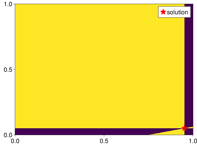
Figure 3: Ratio game. A particularly difficult parametrization ofΒ (5) suggested inΒ [14]. Right: The sign of ⟨F​(u),uβˆ’uβˆ—βŸ©πΉπ‘’π‘’superscript𝑒\langle F(u),u-u^{*}\rangle parametrized as u:=(x,1βˆ’x,y,1βˆ’y)assign𝑒π‘₯1π‘₯𝑦1𝑦u:=(x,1-x,y,1-y), with yellow representing a negative sign and purple a positive one, highlighting the fact that the solution is not Minty. Nevertheless, all methods are able to converge.

We consider von Neumann’s ratio gameΒ [51] recently explored inΒ [14, 18]. It is given by

minxβˆˆΞ”m⁑maxyβˆˆΞ”n⁑V​(x,y)=⟨x,R​y⟩⟨x,S​y⟩,subscriptπ‘₯superscriptΞ”π‘šsubscript𝑦superscriptΔ𝑛𝑉π‘₯𝑦π‘₯𝑅𝑦π‘₯𝑆𝑦\min_{x\in\Delta^{m}}\,\max_{y\in\Delta^{n}}\,V(x,y)=\frac{\langle x,Ry\rangle}{\langle x,Sy\rangle}, (5)

where Rβˆˆβ„mΓ—n𝑅superscriptβ„π‘šπ‘›R\in\mathbb{R}^{m\times n} and Sβˆˆβ„+mΓ—n𝑆superscriptsubscriptβ„π‘šπ‘›S\in\mathbb{R}_{+}^{m\times n} with ⟨x,S​y⟩>0π‘₯𝑆𝑦0\langle x,Sy\rangle>0 for all xβˆˆΞ”m,yβˆˆΞ”nformulae-sequenceπ‘₯superscriptΞ”π‘šπ‘¦superscriptΔ𝑛x\in\Delta^{m},y\in\Delta^{n}, with Ξ”d:={zβˆˆβ„d:ziβ‰₯0,βˆ‘i=1dzi=1}assignsuperscriptΔ𝑑conditional-set𝑧superscriptℝ𝑑formulae-sequencesubscript𝑧𝑖0superscriptsubscript𝑖1𝑑subscript𝑧𝑖1\Delta^{d}:=\{z\in\mathbb{R}^{d}:z_{i}\geq 0,\sum_{i=1}^{d}z_{i}=1\} denoting the unit simplex. ExpressionΒ (5) can be interpreted as the value V​(Ο€x,Ο€y)𝑉subscriptπœ‹π‘₯subscriptπœ‹π‘¦V(\pi_{x},\pi_{y}) for a stochastic game with a single state and mixed strategies.

In Figure 3(b) we see an illustration of a particularly difficult instance of (5) discussed in [14], highlighting the fact that the Stampacchia solution is not a Minty solution, even when restricted to arbitrarily close ball around it (yellow area touching the solution). Interestingly we still observe good convergence behavior, although an estimated ρ𝜌\rho is more than ten times larger than the estimated Lipschitz constant.

5.2 Forsaken

A particularly difficult min-max toy example with β€œForsaken” solution was proposed in Example 5.2 ofΒ [26], and is given by

minxβˆˆβ„β‘maxyβˆˆβ„β‘x​(yβˆ’0.45)+φ​(x)βˆ’Ο†β€‹(y),subscriptπ‘₯ℝsubscript𝑦ℝπ‘₯𝑦0.45πœ‘π‘₯πœ‘π‘¦\min_{x\in\mathbb{R}}\,\max_{y\in\mathbb{R}}\,x(y-0.45)+\varphi(x)-\varphi(y), (6)

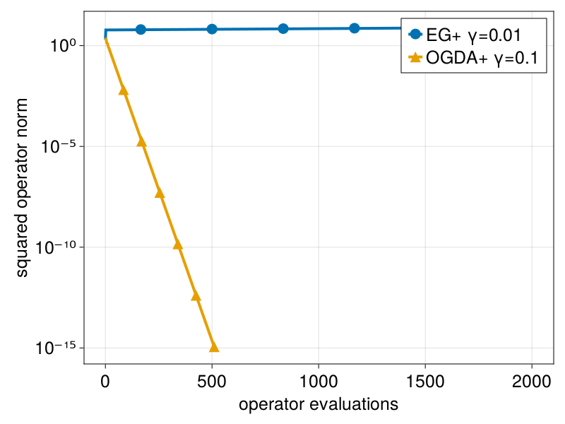
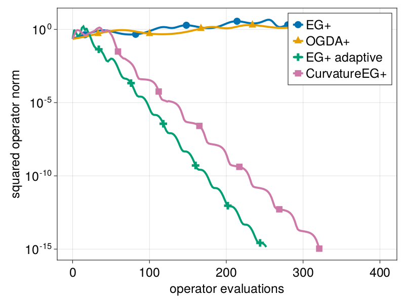
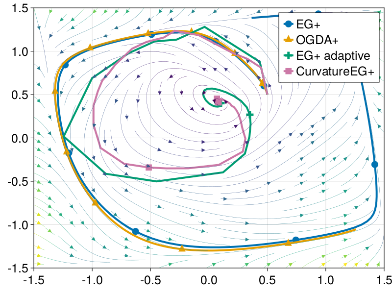
where φ​(z)=14​z2βˆ’12​z4+16​z6πœ‘π‘§14superscript𝑧212superscript𝑧416superscript𝑧6\varphi(z)=\frac{1}{4}z^{2}-\frac{1}{2}z^{4}+\frac{1}{6}z^{6}. This problem exhibits a Stampacchia solution at (xβˆ—,yβˆ—)β‰ˆ(0.08,0.4)superscriptπ‘₯superscript𝑦0.080.4(x^{*},y^{*})\approx(0.08,0.4), but also two limit cycles not containing any critical point of the objective function. In addition,Β [26] also observed that the limit cycle closer to the solution repels possible trajectories of iterates, thus β€œshielding” the solution. Later,Β [44] noticed that, restricted to the box β€–(x,y)β€–βˆž<32subscriptnormπ‘₯𝑦32\|(x,y)\|_{\infty}<\frac{3}{2} the above mentioned solution is weak Minty with ρβ‰₯2β‹…0.477761πœŒβ‹…20.477761\rho\geq 2\cdot 0.477761, which is much larger than 1Lβ‰ˆ0.081𝐿0.08\frac{1}{L}\approx 0.08. In line with these observations we can see in FigureΒ 4 that none of the fixed step size methods with step size bounded by 1L1𝐿\frac{1}{L} converge. In light of this observationΒ [44] proposed a backtracking linesearch which potentially allows for larger steps than predicted by the global Lipschitz constant. Similarly, our proposed adaptive step size version of EG++, see AlgorithmΒ 3, is also able to break through the repelling limit cycle and converge the solution. On top of this, it does so at a faster rate and without the need of additional computations in the backtracking procedure.
Refer to caption
(a) Performance of methods.
Refer to caption
(b) Trajectories of iterates.
Figure 4: Forsaken. An illustration of different methods on problemΒ (6), originally suggested byΒ [26]. Only AlgorithmΒ 3 and CurvatureEG++ are able to choose a step size large enough to withstand the repellent limit cycle.

5.3 Lower bound example

The following min-max problem was introduced in [44] as a lower bound on the dependence between ρ𝜌\rho and L𝐿L for EG++:

minxβˆˆβ„β‘maxyβˆˆβ„β‘ΞΎβ€‹x​y+ΞΆ2​(x2βˆ’y2).subscriptπ‘₯ℝsubscriptπ‘¦β„πœ‰π‘₯π‘¦πœ2superscriptπ‘₯2superscript𝑦2\min_{x\in\mathbb{R}}\,\max_{y\in\mathbb{R}}\,\xi xy+\frac{\zeta}{2}(x^{2}-y^{2}). (7)

In particular Theorem 3.4 fromΒ [44] states that EG++ (with any γ𝛾\gamma) and constant step size a=1Lπ‘Ž1𝐿a=\frac{1}{L} converges for this problem if and only if (0,0)00(0,0) is a weak Minty solution with ρ<1βˆ’Ξ³L𝜌1𝛾𝐿\rho<\frac{1-\gamma}{L}, where ρ𝜌\rho and L𝐿L can be computed explicitly in the above example and are given by

L=ΞΎ2+ΞΆ2andρ=βˆ’2​΢ξ2+ΞΆ2.formulae-sequence𝐿superscriptπœ‰2superscript𝜁2and𝜌2𝜁superscriptπœ‰2superscript𝜁2L=\sqrt{\xi^{2}+\zeta^{2}}\quad\text{and}\quad\rho=-2\frac{\zeta}{\xi^{2}+\zeta^{2}}.

FigureΒ 1 is obtained by choosing ΞΎ=3πœ‰3\xi=\sqrt{3} and ΞΆ=βˆ’1𝜁1\zeta=-1 we get exactly ρ=1L𝜌1𝐿\rho=\frac{1}{L} and the theory therefore predicting divergence of EG++ for any γ𝛾\gamma, which is exactly what is empirically observed. Although, the general upper bound proved in TheoremΒ 3.1 only states convergence in the case ρ<1L𝜌1𝐿\rho<\frac{1}{L}, we observe rapid convergence of OGDA++ for this example showcasing that it can drastically outperform EG++ in some scenarios.

6 Conclusion

Many interesting questions remain in the realm of min-max problems β€” especially when leaving the convex-concave setting. Very recentlyΒ [24] showed that the π’ͺ​(1/k)π’ͺ1π‘˜\mathcal{O}(1/k) bounds on the squared operator norm for EG and OGDA for the last iterate (and not just the best one) hold even in the negative comonotone setting. Deriving a similar statement in the presence of merely weak Minty solutions is an open question.

Overall, our analysis and experiments seem to provide evidence that there is little advantage of using OGDA++ over EG++ for most problems as the lower iteration cost is offset by the smaller step size. One exception is given by problem 7 displayed in FigureΒ 1, which is not covered by theory and OGDA++ is the only method able to converge.

Lastly, we observe that the previous paradigm in pure minimization of β€œsmaller step size ensures convergence” but β€œlarger step size gets there faster”, where the latter is typically constrained by the reciprocal of the gradients Lipschitz constant, does not seem to hold true for min-max problems anymore. The analysis of different methods in the presence of weak Minty solutions shows that convergence can be lost if the step size is too small and sometimes needs to be larger than 1L1𝐿\frac{1}{L}, which one can typically only hope for in adaptive methods. Our EG++ method with adaptive step size achieves this even without the additional cost of a backtracking linesearch as used for the CurvatureEG++ method ofΒ [44].

References

  • [1] Kimon Antonakopoulos, Veronica Belmega, and Panayotis Mertikopoulos. An adaptive mirror-prox method for variational inequalities with singular operators. In H.Β Wallach, H.Β Larochelle, A.Β Beygelzimer, F.Β d'AlchΓ©-Buc, E.Β Fox, and R.Β Garnett, editors, Advances in Neural Information Processing Systems, volumeΒ 32. Curran Associates, Inc., 2019.
  • [2] Kimon Antonakopoulos, Veronica Belmega, and Panayotis Mertikopoulos. Adaptive extra-gradient methods for min-max optimization and games. In International Conference on Learning Representations, 2021.
  • [3] Francis Bach and KfirΒ Y Levy. A universal algorithm for variational inequalities adaptive to smoothness and noise. In Conference on Learning Theory, pages 164–194. PMLR, 2019.
  • [4] HeinzΒ H Bauschke, WalaaΒ M Moursi, and Xianfu Wang. Generalized monotone operators and their averaged resolvents. Mathematical Programming, pages 1–20, 2020.
  • [5] Axel BΓΆhm, Michael Sedlmayer, ErnΓΆΒ Robert Csetnek, and RaduΒ Ioan BoΕ£. Two steps at a time – taking GAN training in stride with Tseng’s method. SIAM Journal on Mathematics of Data Science, 4(2):750–771, 2022.
  • [6] AvishekΒ Joey Bose, Gauthier Gidel, Hugo Berard, Andre Cianflone, Pascal Vincent, Simon Lacoste-Julien, and WilliamΒ L. Hamilton. Adversarial example games. In Hugo Larochelle, Marc’Aurelio Ranzato, Raia Hadsell, Maria-Florina Balcan, and Hsuan-Tien Lin, editors, Advances in Neural Information Processing Systems 33: Annual Conference on Neural Information Processing Systems 2020, NeurIPS 2020, December 6-12, 2020, virtual, 2020.
  • [7] RaduΒ Ioan BoΕ£ and Axel BΓΆhm. Alternating proximal-gradient steps for (stochastic) nonconvex-concave minimax problems. arXiv:2007.13605, 2020.
  • [8] RaduΒ Ioan BoΕ£, Michael Sedlmayer, and PhanΒ Tu Vuong. A relaxed inertial forward-backward-forward algorithm for solving monotone inclusions with application to GANs. arXiv:2003.07886, 2020.
  • [9] Yang Cai, Argyris Oikonomou, and Weiqiang Zheng. Accelerated single-call methods for monotone inclusions and constrained min-max optimization. arXiv preprint arXiv:2206.05248, 2022.
  • [10] Tatjana Chavdarova, MichaelΒ I Jordan, and Manolis Zampetakis. Last-iterate convergence of saddle point optimizers via high-resolution differential equations. arXiv preprint arXiv:2112.13826, 2021.
  • [11] PatrickΒ L Combettes and Teemu Pennanen. Proximal methods for cohypomonotone operators. SIAM journal on control and optimization, 43(2):731–742, 2004.
  • [12] ErnΓΆΒ Robert Csetnek, Yura Malitsky, and MatthewΒ K Tam. Shadow Douglas–Rachford splitting for monotone inclusions. Applied Mathematics & Optimization, 80(3):665–678, 2019.
  • [13] CongΒ D Dang and Guanghui Lan. On the convergence properties of non-euclidean extragradient methods for variational inequalities with generalized monotone operators. Computational Optimization and applications, 60(2):277–310, 2015.
  • [14] Constantinos Daskalakis, DylanΒ J Foster, and Noah Golowich. Independent policy gradient methods for competitive reinforcement learning. In H.Β Larochelle, M.Β Ranzato, R.Β Hadsell, M.Β F. Balcan, and H.Β Lin, editors, Advances in Neural Information Processing Systems, volumeΒ 33, pages 5527–5540. Curran Associates, Inc., 2020.
  • [15] Constantinos Daskalakis, Andrew Ilyas, Vasilis Syrgkanis, and Haoyang Zeng. Training GANs with optimism. In International Conference on Learning Representations, 2018.
  • [16] Constantinos Daskalakis and Ioannis Panageas. The limit points of (optimistic) gradient descent in min-max optimization. In Advances in Neural Information Processing Systems, pages 9236–9246, 2018.
  • [17] Constantinos Daskalakis, Stratis Skoulakis, and Manolis Zampetakis. The complexity of constrained min-max optimization. In Proceedings of the 53rd Annual ACM SIGACT Symposium on Theory of Computing, pages 1466–1478, 2021.
  • [18] Jelena Diakonikolas, Constantinos Daskalakis, and Michael Jordan. Efficient methods for structured nonconvex-nonconcave min-max optimization. In International Conference on Artificial Intelligence and Statistics, pages 2746–2754. PMLR, 2021.
  • [19] Francisco Facchinei and Jong-Shi Pang. Finite-dimensional variational inequalities and complementarity problems. Springer Science & Business Media, 2007.
  • [20] Gauthier Gidel, Hugo Berard, GaΓ«tan Vignoud, Pascal Vincent, and Simon Lacoste-Julien. A variational inequality perspective on generative adversarial networks. In International Conference on Learning Representations, 2019.
  • [21] Ian Goodfellow, Jean Pouget-Abadie, Mehdi Mirza, Bing Xu, David Warde-Farley, Sherjil Ozair, Aaron Courville, and Yoshua Bengio. Generative adversarial nets. In Advances in Neural Information Processing Systems, pages 2672–2680, 2014.
  • [22] Eduard Gorbunov, Nicolas Loizou, and Gauthier Gidel. Extragradient method: O​(1/k)𝑂1π‘˜{O}(1/k) last-iterate convergence for monotone variational inequalities and connections with cocoercivity. In International Conference on Artificial Intelligence and Statistics, pages 366–402. PMLR, 2022.
  • [23] Eduard Gorbunov, Adrien Taylor, and Gauthier Gidel. Last-iterate convergence of optimistic gradient method for monotone variational inequalities. arXiv prprint arXiv:2205.08446, 2022.
  • [24] Eduard Gorbunov, Adrien Taylor, Samuel HorvΓ‘th, and Gauthier Gidel. Convergence of proximal point and extragradient-based methods beyond monotonicity: the case of negative comonotonicity. arXiv preprint arXiv:2210.13831, 2022.
  • [25] Benjamin Grimmer, Haihao Lu, Pratik Worah, and Vahab Mirrokni. The landscape of the proximal point method for nonconvex–nonconcave minimax optimization. Mathematical Programming, pages 1–35, 2022.
  • [26] Ya-Ping Hsieh, Panayotis Mertikopoulos, and Volkan Cevher. The limits of min-max optimization algorithms: Convergence to spurious non-critical sets. In International Conference on Machine Learning, pages 4337–4348. PMLR, 2021.
  • [27] Yu-Guan Hsieh, Franck Iutzeler, JΓ©rΓ΄me Malick, and Panayotis Mertikopoulos. Explore aggressively, update conservatively: Stochastic extragradient methods with variable stepsize scaling. In H.Β Larochelle, M.Β Ranzato, R.Β Hadsell, M.Β F. Balcan, and H.Β Lin, editors, Advances in Neural Information Processing Systems, volumeΒ 33, pages 16223–16234. Curran Associates, Inc., 2020.
  • [28] David Kinderlehrer and Guido Stampacchia. An introduction to variational inequalities and their applications. SIAM, 2000.
  • [29] GMΒ Korpelevich. The extragradient method for finding saddle points and other problems. Matecon, 12:747–756, 1976.
  • [30] Sucheol Lee and Donghwan Kim. Fast extra gradient methods for smooth structured nonconvex-nonconcave minimax problems. In A.Β Beygelzimer, Y.Β Dauphin, P.Β Liang, and J.Β Wortman Vaughan, editors, Advances in Neural Information Processing Systems, 2021.
  • [31] Sucheol Lee and Donghwan Kim. Semi-anchored multi-step gradient descent ascent method for structured nonconvex-nonconcave composite minimax problems. arXiv preprint arXiv:2105.15042, 2021.
  • [32] Tengyuan Liang and James Stokes. Interaction matters: A note on non-asymptotic local convergence of generative adversarial networks. In Kamalika Chaudhuri and Masashi Sugiyama, editors, The 22nd International Conference on Artificial Intelligence and Statistics, volumeΒ 89 of Proceedings of Machine Learning Research, pages 907–915. PMLR, 2019.
  • [33] Tianyi Lin, Chi Jin, and MichaelΒ I Jordan. On gradient descent ascent for nonconvex-concave minimax problems. In International Conference on Machine Learning, pages 6083–6093. PMLR, 2020.
  • [34] Mingrui Liu, Youssef Mroueh, Jerret Ross, Wei Zhang, Xiaodong Cui, Payel Das, and Tianbao Yang. Towards better understanding of adaptive gradient algorithms in generative adversarial nets. In International Conference on Learning Representations, 2020.
  • [35] Mingrui Liu, Hassan Rafique, Qihang Lin, and Tianbao Yang. First-order convergence theory for weakly-convex-weakly-concave min-max problems. The Journal of Machine Learning Research, 2021.
  • [36] Aleksander Madry, Aleksandar Makelov, Ludwig Schmidt, Dimitris Tsipras, and Adrian Vladu. Towards deep learning models resistant to adversarial attacks. In International Conference on Learning Representations, 2018.
  • [37] Yura Malitsky. Projected reflected gradient methods for monotone variational inequalities. SIAM Journal on Optimization, 25(1):502–520, 2015.
  • [38] Yura Malitsky. Golden ratio algorithms for variational inequalities. Mathematical Programming, 184(1):383–410, 2020.
  • [39] Yura Malitsky and MatthewΒ K Tam. A forward-backward splitting method for monotone inclusions without cocoercivity. SIAM Journal on Optimization, 30(2):1451–1472, 2020.
  • [40] Panayotis Mertikopoulos, Bruno Lecouat, Houssam Zenati, Chuan-Sheng Foo, Vijay Chandrasekhar, and Georgios Piliouras. Optimistic mirror descent in saddle-point problems: Going the extra(-gradient) mile. In International Conference on Learning Representations, 2019.
  • [41] Aryan Mokhtari, Asuman Ozdaglar, and Sarath Pattathil. A unified analysis of extra-gradient and optimistic gradient methods for saddle point problems: Proximal point approach. In International Conference on Artificial Intelligence and Statistics, pages 1497–1507. PMLR, 2020.
  • [42] Yurii Nesterov. Dual extrapolation and its applications to solving variational inequalities and related problems. Mathematical Programming, 109(2-3):319–344, 2007.
  • [43] Teemu Pennanen. On the range of monotone composite mappings. Journal of Nonlinear and Convex Analysis, 2(2), 2001.
  • [44] Thomas Pethick, Puya Latafat, Panos Patrinos, Olivier Fercoq, and Volkan Cevher. Escaping limit cycles: Global convergence for constrained nonconvex-nonconcave minimax problems. In International Conference on Learning Representations, 2022.
  • [45] David Pfau and Oriol Vinyals. Connecting generative adversarial networks and actor-critic methods. arXiv preprint arXiv:1610.01945, 2016.
  • [46] LeonidΒ Denisovich Popov. A modification of the arrow-hurwicz method for search of saddle points. Mathematical notes of the Academy of Sciences of the USSR, 28(5):845–848, 1980.
  • [47] Alexander Rakhlin and Karthik Sridharan. Online learning with predictable sequences. In Proceedings of the 26th Annual Conference on Learning Theory, pages 993–1019, 2013.
  • [48] Sasha Rakhlin and Karthik Sridharan. Optimization, learning, and games with predictable sequences. In Advances in Neural Information Processing Systems, pages 3066–3074, 2013.
  • [49] ErnestΒ K Ryu, Kun Yuan, and Wotao Yin. Ode analysis of stochastic gradient methods with optimism and anchoring for minimax problems and GANs. arXiv preprint arXiv:1905.10899, 2019.
  • [50] Paul Tseng. A modified forward-backward splitting method for maximal monotone mappings. SIAM Journal on Control and Optimization, 38(2):431–446, 2000.
  • [51] John von Neumann. A model of general economic equilibrium. The Review of Economic Studies, 13(1):1–9, 1945.
  • [52] ZiΒ Xu, Huiling Zhang, Yang Xu, and Guanghui Lan. A unified single-loop alternating gradient projection algorithm for nonconvex–concave and convex–nonconcave minimax problems. Mathematical Programming, pages 1–72, 2023.
  • [53] Jun Yang and Hongwei Liu. A modified projected gradient method for monotone variational inequalities. Journal of Optimization Theory and Applications, 179(1):197–211, 2018.
  • [54] Junchi Yang, Negar Kiyavash, and Niao He. Global convergence and variance-reduced optimization for a class of nonconvex-nonconcave minimax problems. arXiv preprint arXiv:2002.09621, 2020.

Appendix A Omitted proofs

A.1 OGDA++

For convenience we will sometimes use the notation gksubscriptπ‘”π‘˜g_{k} for F​(uk)𝐹subscriptπ‘’π‘˜F(u_{k}) for all kβ‰₯βˆ’1π‘˜1k\geq-1.

Lemma A.1.

Let (uk)subscriptπ‘’π‘˜(u_{k}) be the sequence of iterates generated by AlgorithmΒ 1, then

β€–uk+1+a​gkβˆ’uβˆ—β€–2superscriptnormsubscriptπ‘’π‘˜1π‘Žsubscriptπ‘”π‘˜superscript𝑒2\displaystyle\|u_{k+1}+ag_{k}-u^{*}\|^{2} ≀‖uk+a​gkβˆ’1βˆ’uβˆ—β€–2+a​γ​ρ​‖gkβ€–2+4​aβ€‹Ξ³βˆ’1β€‹βŸ¨gkβˆ’gkβˆ’1,ukβˆ’uk+1⟩absentsuperscriptnormsubscriptπ‘’π‘˜π‘Žsubscriptπ‘”π‘˜1superscript𝑒2π‘Žπ›ΎπœŒsuperscriptnormsubscriptπ‘”π‘˜24π‘Žsuperscript𝛾1subscriptπ‘”π‘˜subscriptπ‘”π‘˜1subscriptπ‘’π‘˜subscriptπ‘’π‘˜1\displaystyle\leq\|u_{k}+ag_{k-1}-u^{*}\|^{2}+a\gamma\rho\|g_{k}\|^{2}+4a\gamma^{-1}\langle g_{k}-g_{k-1},u_{k}-u_{k+1}\rangle (8)
βˆ’(2β€‹Ξ³βˆ’1βˆ’1)​‖uk+1βˆ’ukβ€–2βˆ’a2​(1+2β€‹Ξ³βˆ’1)​‖gkβˆ’gkβˆ’1β€–2.2superscript𝛾11superscriptnormsubscriptπ‘’π‘˜1subscriptπ‘’π‘˜2superscriptπ‘Ž212superscript𝛾1superscriptnormsubscriptπ‘”π‘˜subscriptπ‘”π‘˜12\displaystyle\quad-(2\gamma^{-1}-1)\|u_{k+1}-u_{k}\|^{2}-a^{2}(1+2\gamma^{-1})\|g_{k}-g_{k-1}\|^{2}.
Proof.

From the update of the method we deduce for all kβ‰₯0π‘˜0k\geq 0

β€–uk+1+a​gkβˆ’uβˆ—β€–2superscriptnormsubscriptπ‘’π‘˜1π‘Žsubscriptπ‘”π‘˜superscript𝑒2\displaystyle\|u_{k+1}+ag_{k}-u^{*}\|^{2} =β€–ukβˆ’a​γ​gk+a​gkβˆ’1βˆ’uβˆ—β€–2absentsuperscriptnormsubscriptπ‘’π‘˜π‘Žπ›Ύsubscriptπ‘”π‘˜π‘Žsubscriptπ‘”π‘˜1superscript𝑒2\displaystyle=\|u_{k}-a\gamma g_{k}+ag_{k-1}-u^{*}\|^{2} (9)
=β€–uk+a​gkβˆ’1βˆ’uβˆ—β€–2βˆ’2β€‹βŸ¨ukβˆ’uβˆ—,a​γ​gkβŸ©βˆ’βŸ¨2​a​gkβˆ’1βˆ’a​γ​gk,a​γ​gk⟩absentsuperscriptnormsubscriptπ‘’π‘˜π‘Žsubscriptπ‘”π‘˜1superscript𝑒22subscriptπ‘’π‘˜superscriptπ‘’π‘Žπ›Ύsubscriptπ‘”π‘˜2π‘Žsubscriptπ‘”π‘˜1π‘Žπ›Ύsubscriptπ‘”π‘˜π‘Žπ›Ύsubscriptπ‘”π‘˜\displaystyle=\|u_{k}+ag_{k-1}-u^{*}\|^{2}-2\langle u_{k}-u^{*},a\gamma g_{k}\rangle-\langle 2ag_{k-1}-a\gamma g_{k},a\gamma g_{k}\rangle
≀‖uk+a​gkβˆ’1βˆ’uβˆ—β€–2+a​γ​ρ​‖gkβ€–2βˆ’βŸ¨2​a​gkβˆ’1βˆ’a​γ​gk,a​γ​gk⟩,absentsuperscriptnormsubscriptπ‘’π‘˜π‘Žsubscriptπ‘”π‘˜1superscript𝑒2π‘Žπ›ΎπœŒsuperscriptnormsubscriptπ‘”π‘˜22π‘Žsubscriptπ‘”π‘˜1π‘Žπ›Ύsubscriptπ‘”π‘˜π‘Žπ›Ύsubscriptπ‘”π‘˜\displaystyle\leq\|u_{k}+ag_{k-1}-u^{*}\|^{2}+a\gamma\rho\|g_{k}\|^{2}-\langle 2ag_{k-1}-a\gamma g_{k},a\gamma g_{k}\rangle,

where we used the weak Minty assumption to deduce the last inequality. It remains to derive the following equality

βˆ’βŸ¨2​a​gkβˆ’1βˆ’a​γ​gk,a​γ​gk⟩=4​aβ€‹Ξ³βˆ’1β€‹βŸ¨gkβˆ’gkβˆ’1,ukβˆ’uk+1βŸ©βˆ’(2β€‹Ξ³βˆ’1βˆ’1)​‖uk+1βˆ’ukβ€–2βˆ’a2​(1+2β€‹Ξ³βˆ’1)​‖gkβˆ’gkβˆ’1β€–2.2π‘Žsubscriptπ‘”π‘˜1π‘Žπ›Ύsubscriptπ‘”π‘˜π‘Žπ›Ύsubscriptπ‘”π‘˜4π‘Žsuperscript𝛾1subscriptπ‘”π‘˜subscriptπ‘”π‘˜1subscriptπ‘’π‘˜subscriptπ‘’π‘˜12superscript𝛾11superscriptdelimited-βˆ₯βˆ₯subscriptπ‘’π‘˜1subscriptπ‘’π‘˜2superscriptπ‘Ž212superscript𝛾1superscriptdelimited-βˆ₯βˆ₯subscriptπ‘”π‘˜subscriptπ‘”π‘˜12\begin{split}-\langle 2ag_{k-1}-a\gamma g_{k},a\gamma g_{k}\rangle=4a\gamma^{-1}\langle g_{k}-g_{k-1},u_{k}-u_{k+1}\rangle-(2\gamma^{-1}-1)\|u_{k+1}-u_{k}\|^{2}\\ -a^{2}(1+2\gamma^{-1})\|g_{k}-g_{k-1}\|^{2}.\end{split} (10)

This can be seen by expressing every difference of iterates in terms of gradients according to AlgorithmΒ 1, giving

4​aβ€‹Ξ³βˆ’1β€‹βŸ¨gkβˆ’gkβˆ’1,ukβˆ’uk+1⟩4π‘Žsuperscript𝛾1subscriptπ‘”π‘˜subscriptπ‘”π‘˜1subscriptπ‘’π‘˜subscriptπ‘’π‘˜1\displaystyle 4a\gamma^{-1}\langle g_{k}-g_{k-1},u_{k}-u_{k+1}\rangle =4​aβ€‹Ξ³βˆ’1β€‹βŸ¨gkβˆ’gkβˆ’1,a​(gkβˆ’gkβˆ’1)+a​γ​gk⟩absent4π‘Žsuperscript𝛾1subscriptπ‘”π‘˜subscriptπ‘”π‘˜1π‘Žsubscriptπ‘”π‘˜subscriptπ‘”π‘˜1π‘Žπ›Ύsubscriptπ‘”π‘˜\displaystyle=4a\gamma^{-1}\langle g_{k}-g_{k-1},a(g_{k}-g_{k-1})+a\gamma g_{k}\rangle
=4​a2β€‹Ξ³βˆ’1​‖gkβˆ’gkβˆ’1β€–2+4​a2β€‹βŸ¨gk,gkβˆ’gkβˆ’1⟩absent4superscriptπ‘Ž2superscript𝛾1superscriptnormsubscriptπ‘”π‘˜subscriptπ‘”π‘˜124superscriptπ‘Ž2subscriptπ‘”π‘˜subscriptπ‘”π‘˜subscriptπ‘”π‘˜1\displaystyle=4a^{2}\gamma^{-1}\|g_{k}-g_{k-1}\|^{2}+4a^{2}\langle g_{k},g_{k}-g_{k-1}\rangle

and

βˆ’(2β€‹Ξ³βˆ’1βˆ’1)​‖uk+1βˆ’ukβ€–22superscript𝛾11superscriptnormsubscriptπ‘’π‘˜1subscriptπ‘’π‘˜2\displaystyle-(2\gamma^{-1}-1)\|u_{k+1}-u_{k}\|^{2}
=(1βˆ’2β€‹Ξ³βˆ’1)​‖a​(gkβˆ’gkβˆ’1)+a​γ​gkβ€–2absent12superscript𝛾1superscriptnormπ‘Žsubscriptπ‘”π‘˜subscriptπ‘”π‘˜1π‘Žπ›Ύsubscriptπ‘”π‘˜2\displaystyle=(1-2\gamma^{-1})\|a(g_{k}-g_{k-1})+a\gamma g_{k}\|^{2}
=(a2βˆ’2​a2β€‹Ξ³βˆ’1)​‖gkβˆ’gkβˆ’1β€–2+(2​γ​a2βˆ’4​a2)β€‹βŸ¨gk,gkβˆ’gkβˆ’1⟩+(a2​γ2βˆ’2​a2​γ)​‖gkβ€–2absentsuperscriptπ‘Ž22superscriptπ‘Ž2superscript𝛾1superscriptnormsubscriptπ‘”π‘˜subscriptπ‘”π‘˜122𝛾superscriptπ‘Ž24superscriptπ‘Ž2subscriptπ‘”π‘˜subscriptπ‘”π‘˜subscriptπ‘”π‘˜1superscriptπ‘Ž2superscript𝛾22superscriptπ‘Ž2𝛾superscriptnormsubscriptπ‘”π‘˜2\displaystyle=(a^{2}-2a^{2}\gamma^{-1})\|g_{k}-g_{k-1}\|^{2}+(2\gamma a^{2}-4a^{2})\langle g_{k},g_{k}-g_{k-1}\rangle+(a^{2}\gamma^{2}-2a^{2}\gamma)\|g_{k}\|^{2}
=(a2βˆ’2​a2β€‹Ξ³βˆ’1)​‖gkβˆ’gkβˆ’1β€–2+⟨gk,(a2​γ2βˆ’4​a2)​gkβˆ’(2​γ​a2βˆ’4​a2)​gkβˆ’1⟩.absentsuperscriptπ‘Ž22superscriptπ‘Ž2superscript𝛾1superscriptnormsubscriptπ‘”π‘˜subscriptπ‘”π‘˜12subscriptπ‘”π‘˜superscriptπ‘Ž2superscript𝛾24superscriptπ‘Ž2subscriptπ‘”π‘˜2𝛾superscriptπ‘Ž24superscriptπ‘Ž2subscriptπ‘”π‘˜1\displaystyle=(a^{2}-2a^{2}\gamma^{-1})\|g_{k}-g_{k-1}\|^{2}+\langle g_{k},(a^{2}\gamma^{2}-4a^{2})g_{k}-(2\gamma a^{2}-4a^{2})g_{k-1}\rangle.

Adding the previous two equalities to βˆ’a2​(1+2β€‹Ξ³βˆ’1)​‖gkβˆ’gkβˆ’1β€–2superscriptπ‘Ž212superscript𝛾1superscriptnormsubscriptπ‘”π‘˜subscriptπ‘”π‘˜12-a^{2}(1+2\gamma^{-1})\|g_{k}-g_{k-1}\|^{2} provesΒ (10). Combining 9 andΒ 10 proves the desired statement. ∎

We are actually going to show a slightly more general version of TheoremΒ 3.1, which introduces an additional parameter Ξ»πœ†\lambda. Note that for Ξ»=Ξ³βˆ’1πœ†superscript𝛾1\lambda=\gamma^{-1} we recover the statement of TheoremΒ 3.1. This allows us to cover the analysis of the monotone case in one proof. In particular Ξ»πœ†\lambda close to zero will yield the statement of TheoremΒ 3.2.

Theorem A.1.

Let F:ℝd→ℝd:𝐹→superscriptℝ𝑑superscriptℝ𝑑F:\mathbb{R}^{d}\to\mathbb{R}^{d} be L𝐿L-Lipschitz continuous satisfying AssumptionΒ 1, where uβˆ—superscript𝑒u^{*} denotes any weak Minty solution, with a​λ​γ>Οπ‘Žπœ†π›ΎπœŒa\lambda\gamma>\rho for some 0≀λ≀2β€‹Ξ³βˆ’10πœ†2superscript𝛾10\leq\lambda\leq 2\gamma^{-1} and let (uk)kβ‰₯0subscriptsubscriptπ‘’π‘˜π‘˜0{(u_{k})}_{k\geq 0} be the sequence of iterates generated by AlgorithmΒ 1 with

a​L≀2βˆ’Ξ»β€‹Ξ³βˆ’Ξ³2βˆ’Ξ»β€‹Ξ³+Ξ³.π‘ŽπΏ2πœ†π›Ύπ›Ύ2πœ†π›Ύπ›ΎaL\leq\frac{2-\lambda\gamma-\gamma}{2-\lambda\gamma+\gamma}. (11)

Then, for all kβ‰₯0π‘˜0k\geq 0

1kβ€‹βˆ‘i=0kβˆ’1β€–F​(ui)β€–2≀1k​a​γ​(aβ€‹Ξ»β€‹Ξ³βˆ’Ο)​‖u0+a​F​(u0)βˆ’uβˆ—β€–2.1π‘˜superscriptsubscript𝑖0π‘˜1superscriptnorm𝐹subscript𝑒𝑖21π‘˜π‘Žπ›Ύπ‘Žπœ†π›ΎπœŒsuperscriptnormsubscript𝑒0π‘ŽπΉsubscript𝑒0superscript𝑒2\frac{1}{k}\sum_{i=0}^{k-1}\|F(u_{i})\|^{2}\leq\frac{1}{ka\gamma(a\lambda\gamma-\rho)}\|u_{0}+aF(u_{0})-u^{*}\|^{2}.

In particular as long as ρ<1L𝜌1𝐿\rho<\frac{1}{L} we can find a small enough γ𝛾\gamma such that the above bound holds.

Proof.

Using the definition uk+1subscriptπ‘’π‘˜1u_{k+1} we can express

a​γ​gk=ukβˆ’uk+1βˆ’a​λ​(gkβˆ’gkβˆ’1).π‘Žπ›Ύsubscriptπ‘”π‘˜subscriptπ‘’π‘˜subscriptπ‘’π‘˜1π‘Žπœ†subscriptπ‘”π‘˜subscriptπ‘”π‘˜1a\gamma g_{k}=u_{k}-u_{k+1}-a\lambda(g_{k}-g_{k-1}). (12)

By applying norms on both sides we obtain via expansion of squares

a2​λ​γ2​‖gkβ€–2=λ​‖uk+1βˆ’ukβ€–2+a2​λ​‖gkβˆ’gkβˆ’1β€–2+2​aβ€‹Ξ»β€‹βŸ¨uk+1βˆ’uk,gkβˆ’gkβˆ’1⟩.superscriptπ‘Ž2πœ†superscript𝛾2superscriptnormsubscriptπ‘”π‘˜2πœ†superscriptnormsubscriptπ‘’π‘˜1subscriptπ‘’π‘˜2superscriptπ‘Ž2πœ†superscriptnormsubscriptπ‘”π‘˜subscriptπ‘”π‘˜122π‘Žπœ†subscriptπ‘’π‘˜1subscriptπ‘’π‘˜subscriptπ‘”π‘˜subscriptπ‘”π‘˜1a^{2}\lambda\gamma^{2}\|g_{k}\|^{2}=\lambda\|u_{k+1}-u_{k}\|^{2}+a^{2}\lambda\|g_{k}-g_{k-1}\|^{2}+2a\lambda\langle u_{k+1}-u_{k},g_{k}-g_{k-1}\rangle. (13)

Adding 13 andΒ A.1 we deduce

β€–uk+1+a​gkβˆ’uβˆ—β€–2+a​γ​(aβ€‹Ξ»β€‹Ξ³βˆ’Ο)​‖gkβ€–2≀‖uk+a​gkβˆ’1βˆ’uβˆ—β€–2βˆ’a2​(1+2β€‹Ξ³βˆ’1βˆ’Ξ»)​‖gkβˆ’gkβˆ’1β€–2βˆ’(2β€‹Ξ³βˆ’1βˆ’1βˆ’Ξ»)​‖uk+1βˆ’ukβ€–2+(4​aβ€‹Ξ³βˆ’1βˆ’2​a​λ)β€‹βŸ¨ukβˆ’uk+1,gkβˆ’gkβˆ’1⟩.superscriptdelimited-βˆ₯βˆ₯subscriptπ‘’π‘˜1π‘Žsubscriptπ‘”π‘˜superscript𝑒2π‘Žπ›Ύπ‘Žπœ†π›ΎπœŒsuperscriptdelimited-βˆ₯βˆ₯subscriptπ‘”π‘˜2superscriptdelimited-βˆ₯βˆ₯subscriptπ‘’π‘˜π‘Žsubscriptπ‘”π‘˜1superscript𝑒2superscriptπ‘Ž212superscript𝛾1πœ†superscriptdelimited-βˆ₯βˆ₯subscriptπ‘”π‘˜subscriptπ‘”π‘˜122superscript𝛾11πœ†superscriptdelimited-βˆ₯βˆ₯subscriptπ‘’π‘˜1subscriptπ‘’π‘˜24π‘Žsuperscript𝛾12π‘Žπœ†subscriptπ‘’π‘˜subscriptπ‘’π‘˜1subscriptπ‘”π‘˜subscriptπ‘”π‘˜1\|u_{k+1}+ag_{k}-u^{*}\|^{2}+a\gamma(a\lambda\gamma-\rho)\|g_{k}\|^{2}\leq\|u_{k}+ag_{k-1}-u^{*}\|^{2}-a^{2}(1+2\gamma^{-1}-\lambda)\|g_{k}-g_{k-1}\|^{2}\\ -(2\gamma^{-1}-1-\lambda)\|u_{k+1}-u_{k}\|^{2}+(4a\gamma^{-1}-2a\lambda)\langle u_{k}-u_{k+1},g_{k}-g_{k-1}\rangle. (14)

Now, we get via Young’s inequality

(4β€‹Ξ³βˆ’1​aβˆ’2​a​λ)β€‹βŸ¨ukβˆ’uk+1,gkβˆ’gkβˆ’1βŸ©β‰€a​L​(2β€‹Ξ³βˆ’1βˆ’Ξ»)​‖ukβˆ’uk+1β€–2+Lβˆ’1​a​(2β€‹Ξ³βˆ’1βˆ’Ξ»)​‖gkβˆ’gkβˆ’1β€–2.4superscript𝛾1π‘Ž2π‘Žπœ†subscriptπ‘’π‘˜subscriptπ‘’π‘˜1subscriptπ‘”π‘˜subscriptπ‘”π‘˜1π‘ŽπΏ2superscript𝛾1πœ†superscriptnormsubscriptπ‘’π‘˜subscriptπ‘’π‘˜12superscript𝐿1π‘Ž2superscript𝛾1πœ†superscriptnormsubscriptπ‘”π‘˜subscriptπ‘”π‘˜12(4\gamma^{-1}a-2a\lambda)\langle u_{k}-u_{k+1},g_{k}-g_{k-1}\rangle\leq aL(2\gamma^{-1}-\lambda)\|u_{k}-u_{k+1}\|^{2}+L^{-1}a(2\gamma^{-1}-\lambda)\|g_{k}-g_{k-1}\|^{2}.

Combining the previous two inequalities

β€–uk+1+a​gkβˆ’uβˆ—β€–2+a​γ​(aβ€‹Ξ³β€‹Ξ»βˆ’Ο)​‖gkβ€–2≀‖uk+a​gkβˆ’1βˆ’uβˆ—β€–2+(a​Lβˆ’1​(2β€‹Ξ³βˆ’1βˆ’Ξ»)βˆ’a2​(1+2β€‹Ξ³βˆ’1βˆ’Ξ»))​‖gkβˆ’gkβˆ’1β€–2βˆ’(2β€‹Ξ³βˆ’1βˆ’1βˆ’Ξ»βˆ’L​a​(2β€‹Ξ³βˆ’1βˆ’Ξ»))​‖uk+1βˆ’ukβ€–2.superscriptdelimited-βˆ₯βˆ₯subscriptπ‘’π‘˜1π‘Žsubscriptπ‘”π‘˜superscript𝑒2π‘Žπ›Ύπ‘Žπ›Ύπœ†πœŒsuperscriptdelimited-βˆ₯βˆ₯subscriptπ‘”π‘˜2superscriptdelimited-βˆ₯βˆ₯subscriptπ‘’π‘˜π‘Žsubscriptπ‘”π‘˜1superscript𝑒2π‘Žsuperscript𝐿12superscript𝛾1πœ†superscriptπ‘Ž212superscript𝛾1πœ†superscriptdelimited-βˆ₯βˆ₯subscriptπ‘”π‘˜subscriptπ‘”π‘˜122superscript𝛾11πœ†πΏπ‘Ž2superscript𝛾1πœ†superscriptdelimited-βˆ₯βˆ₯subscriptπ‘’π‘˜1subscriptπ‘’π‘˜2\|u_{k+1}+ag_{k}-u^{*}\|^{2}+a\gamma(a\gamma\lambda-\rho)\|g_{k}\|^{2}\leq\|u_{k}+ag_{k-1}-u^{*}\|^{2}\\ +(aL^{-1}(2\gamma^{-1}-\lambda)-a^{2}(1+2\gamma^{-1}-\lambda))\|g_{k}-g_{k-1}\|^{2}-(2\gamma^{-1}-1-\lambda-La(2\gamma^{-1}-\lambda))\|u_{k+1}-u_{k}\|^{2}. (15)

We now use the Lipschitz continuity222Strictly speaking we would have to assume that the term before β€–gkβˆ’gkβˆ’1β€–2superscriptnormsubscriptπ‘”π‘˜subscriptπ‘”π‘˜12\|g_{k}-g_{k-1}\|^{2} is positive, but if it is not we can just discard it and be done with the proof. of F𝐹F to deduce that

β€–uk+1+a​gkβˆ’uβˆ—β€–2+a​γ​(aβ€‹Ξ³β€‹Ξ»βˆ’Ο)​‖gkβ€–2≀‖uk+a​gkβˆ’1βˆ’uβˆ—β€–2+(a​L​(2β€‹Ξ³βˆ’1βˆ’Ξ»)βˆ’a2​L2​(1+2β€‹Ξ³βˆ’1βˆ’Ξ»))​‖ukβˆ’ukβˆ’1β€–2βˆ’(2β€‹Ξ³βˆ’1βˆ’1βˆ’Ξ»βˆ’L​a​(2β€‹Ξ³βˆ’1βˆ’Ξ»))​‖uk+1βˆ’ukβ€–2.superscriptdelimited-βˆ₯βˆ₯subscriptπ‘’π‘˜1π‘Žsubscriptπ‘”π‘˜superscript𝑒2π‘Žπ›Ύπ‘Žπ›Ύπœ†πœŒsuperscriptdelimited-βˆ₯βˆ₯subscriptπ‘”π‘˜2superscriptdelimited-βˆ₯βˆ₯subscriptπ‘’π‘˜π‘Žsubscriptπ‘”π‘˜1superscript𝑒2π‘ŽπΏ2superscript𝛾1πœ†superscriptπ‘Ž2superscript𝐿212superscript𝛾1πœ†superscriptdelimited-βˆ₯βˆ₯subscriptπ‘’π‘˜subscriptπ‘’π‘˜122superscript𝛾11πœ†πΏπ‘Ž2superscript𝛾1πœ†superscriptdelimited-βˆ₯βˆ₯subscriptπ‘’π‘˜1subscriptπ‘’π‘˜2\|u_{k+1}+ag_{k}-u^{*}\|^{2}+a\gamma(a\gamma\lambda-\rho)\|g_{k}\|^{2}\leq\|u_{k}+ag_{k-1}-u^{*}\|^{2}\\ +(aL(2\gamma^{-1}-\lambda)-a^{2}L^{2}(1+2\gamma^{-1}-\lambda))\|u_{k}-u_{k-1}\|^{2}-(2\gamma^{-1}-1-\lambda-La(2\gamma^{-1}-\lambda))\|u_{k+1}-u_{k}\|^{2}.

The fact that the terms can be telescoped is, with Ξ±=L​aπ›ΌπΏπ‘Ž\alpha=La equivalent to

2β€‹Ξ³βˆ’1βˆ’1βˆ’Ξ»βˆ’(2β€‹Ξ±β€‹Ξ³βˆ’1βˆ’Ξ±β€‹Ξ»)β‰₯βˆ’Ξ±2​(1+2β€‹Ξ³βˆ’1)+Ξ±2​λ+(2β€‹Ξ±β€‹Ξ³βˆ’1βˆ’Ξ±β€‹Ξ»)2superscript𝛾11πœ†2𝛼superscript𝛾1π›Όπœ†superscript𝛼212superscript𝛾1superscript𝛼2πœ†2𝛼superscript𝛾1π›Όπœ†2\gamma^{-1}-1-\lambda-(2\alpha\gamma^{-1}-\alpha\lambda)\geq-\alpha^{2}(1+2\gamma^{-1})+\alpha^{2}\lambda+(2\alpha\gamma^{-1}-\alpha\lambda)

which can be simplified to

Ξ±2​(2+Ξ³βˆ’Ξ»β€‹Ξ³)βˆ’Ξ±β€‹(4βˆ’2​λ​γ)+2βˆ’Ξ³βˆ’Ξ»β€‹Ξ³β‰₯0superscript𝛼22π›Ύπœ†π›Ύπ›Ό42πœ†π›Ύ2π›Ύπœ†π›Ύ0\alpha^{2}(2+\gamma-\lambda\gamma)-\alpha(4-2\lambda\gamma)+2-\gamma-\lambda\gamma\geq 0

By solving for α𝛼\alpha we get the condition

α≀2βˆ’Ξ»β€‹Ξ³βˆ’Ξ³2βˆ’Ξ»β€‹Ξ³+Ξ³,𝛼2πœ†π›Ύπ›Ύ2πœ†π›Ύπ›Ύ\alpha\leq\frac{2-\lambda\gamma-\gamma}{2-\lambda\gamma+\gamma}, (16)

where from the condition 2β€‹Ξ³βˆ’1βˆ’1βˆ’Ξ»βˆ’(2β€‹Ξ±β€‹Ξ³βˆ’1βˆ’Ξ±β€‹Ξ»)β‰₯02superscript𝛾11πœ†2𝛼superscript𝛾1π›Όπœ†02\gamma^{-1}-1-\lambda-(2\alpha\gamma^{-1}-\alpha\lambda)\geq 0 we deduce α≀2βˆ’Ξ»β€‹Ξ³βˆ’Ξ³2βˆ’Ξ»β€‹Ξ³π›Ό2πœ†π›Ύπ›Ύ2πœ†π›Ύ\alpha\leq\frac{2-\lambda\gamma-\gamma}{2-\lambda\gamma}, which is redundant in light of 16. The statement follows since we chose u0=uβˆ’1subscript𝑒0subscript𝑒1u_{0}=u_{-1}. ∎

A.2 Improved bounds under monotonicity

For the readers convenience we restate the theorem from the main text.

Theorem 3.2.

Let F:ℝd→ℝd:𝐹→superscriptℝ𝑑superscriptℝ𝑑F:\mathbb{R}^{d}\to\mathbb{R}^{d} be monotone and L𝐿L-Lipschitz. If a​L=2βˆ’Ξ³2+Ξ³βˆ’Ξ΅π‘ŽπΏ2𝛾2π›Ύπœ€aL=\frac{2-\gamma}{2+\gamma}-\varepsilon for Ξ΅>0πœ€0\varepsilon>0 then, the iterates generated by OGDA++ fulfill

1kβ€‹βˆ‘i=0kβˆ’1β€–F​(ui)β€–2≀2k​a2​γ2​Ρ​‖u0+a​F​(u0)βˆ’uβˆ—β€–2.1π‘˜superscriptsubscript𝑖0π‘˜1superscriptnorm𝐹subscript𝑒𝑖22π‘˜superscriptπ‘Ž2superscript𝛾2πœ€superscriptnormsubscript𝑒0π‘ŽπΉsubscript𝑒0superscript𝑒2\frac{1}{k}\sum_{i=0}^{k-1}\|F(u_{i})\|^{2}\leq\frac{2}{ka^{2}\gamma^{2}\varepsilon}\|u_{0}+aF(u_{0})-u^{*}\|^{2}.

In particular, we can choose Ξ³=1𝛾1\gamma=1 and a<13​Lπ‘Ž13𝐿a<\frac{1}{3L}.

Proof of TheoremΒ 3.2.

From TheoremΒ A.1 and the fact that a​L=Ξ³βˆ’2Ξ³+2βˆ’Ξ΅π‘ŽπΏπ›Ύ2𝛾2πœ€aL=\frac{\gamma-2}{\gamma+2}-\varepsilon we need to find an appropriate Ξ»>0πœ†0\lambda>0 such that a​L≀2βˆ’Ξ»β€‹Ξ³βˆ’Ξ³2βˆ’Ξ»β€‹Ξ³+Ξ³π‘ŽπΏ2πœ†π›Ύπ›Ύ2πœ†π›Ύπ›ΎaL\leq\frac{2-\lambda\gamma-\gamma}{2-\lambda\gamma+\gamma}. Given Ξ΅>0πœ€0\varepsilon>0 we therefore aim to find a Ξ»>0πœ†0\lambda>0 such that

2βˆ’Ξ³2+Ξ³βˆ’Ξ΅β€‹β‰€!​2βˆ’Ξ»β€‹Ξ³βˆ’Ξ³2βˆ’Ξ»β€‹Ξ³+Ξ³.2𝛾2π›Ύπœ€2πœ†π›Ύπ›Ύ2πœ†π›Ύπ›Ύ\frac{2-\gamma}{2+\gamma}-\varepsilon\overset{!}{\leq}\frac{2-\lambda\gamma-\gamma}{2-\lambda\gamma+\gamma}. (17)

By bringing both terms on one side and the same denominator we obtain the condition

2​λ​γ2(Ξ³+2)​(Ξ³+2βˆ’Ξ»β€‹Ξ³)​≀!​Ρ.2πœ†superscript𝛾2𝛾2𝛾2πœ†π›Ύπœ€\frac{2\lambda\gamma^{2}}{(\gamma+2)(\gamma+2-\lambda\gamma)}\overset{!}{\leq}\varepsilon. (18)

Using the fact that λ≀2β€‹Ξ³βˆ’1πœ†2superscript𝛾1\lambda\leq 2\gamma^{-1} and Ξ³β‰₯0𝛾0\gamma\geq 0 we can upper bound the left hand side by Ξ»πœ†\lambda. Choosing Ξ»=Ξ΅πœ†πœ€\lambda=\varepsilon therefore ensures that the necessary condition on the step sizeΒ (16) is satisfied and at the same time yields the dependence on Ξ΅πœ€\varepsilon in the denominator of the right hand side in the statement of the theorem.

∎

A.3 OGDA++ stochastic

For the stochastic analysis we use for convenience the notation Ξ”k+1=𝔼​[β€–uk+1βˆ’ukβ€–2]subscriptΞ”π‘˜1𝔼delimited-[]superscriptnormsubscriptπ‘’π‘˜1subscriptπ‘’π‘˜2\Delta_{k+1}=\mathbb{E}\left[\|u_{k+1}-u_{k}\|^{2}\right] and Οƒ~2=𝔼​[β€–1Bβ€‹βˆ‘j=1BF~​(uk,ΞΎj)βˆ’F​(uk)β€–2]superscript~𝜎2𝔼delimited-[]superscriptnorm1𝐡superscriptsubscript𝑗1𝐡~𝐹subscriptπ‘’π‘˜subscriptπœ‰π‘—πΉsubscriptπ‘’π‘˜2\tilde{\sigma}^{2}=\mathbb{E}\left[\|\frac{1}{B}\sum_{j=1}^{B}\tilde{F}(u_{k},\xi_{j})-F(u_{k})\|^{2}\right].

Lemma A.2.

Let (uk)subscriptπ‘’π‘˜(u_{k}) be the sequence of iterates generated by stochastic OGDA++, then, for any Ξ»>0πœ†0\lambda>0

Lk+1+a​γ​(aβˆ’Ο)​𝔼​[β€–gkβ€–2]≀Lk+2​(1+Ξ»)​C~1​σ~+(1+Ξ»βˆ’1)​C~1​Δkβˆ’C~2​Δk+1.subscriptπΏπ‘˜1π‘Žπ›Ύπ‘ŽπœŒπ”Όdelimited-[]superscriptnormsubscriptπ‘”π‘˜2subscriptπΏπ‘˜21πœ†subscript~𝐢1~𝜎1superscriptπœ†1subscript~𝐢1subscriptΞ”π‘˜subscript~𝐢2subscriptΞ”π‘˜1L_{k+1}+a\gamma(a-\rho)\mathbb{E}\left[\|g_{k}\|^{2}\right]\leq L_{k}+2(1+\lambda)\tilde{C}_{1}\tilde{\sigma}+(1+\lambda^{-1})\tilde{C}_{1}\Delta_{k}-\tilde{C}_{2}\Delta_{k+1}.

where C~1:=max⁑{0,a​Lβ€‹Ξ³βˆ’1βˆ’a2​L2​(1+Ξ³βˆ’1)}assignsubscript~𝐢10π‘ŽπΏsuperscript𝛾1superscriptπ‘Ž2superscript𝐿21superscript𝛾1\tilde{C}_{1}:=\max\{0,aL\gamma^{-1}-a^{2}L^{2}(1+\gamma^{-1})\} and C~2:=Ξ³βˆ’1βˆ’1βˆ’a​Lβ€‹Ξ³βˆ’1assignsubscript~𝐢2superscript𝛾11π‘ŽπΏsuperscript𝛾1\tilde{C}_{2}:=\gamma^{-1}-1-aL\gamma^{-1}.

Proof of LemmaΒ A.2.

From the update of the method we deduce for all kβ‰₯0π‘˜0k\geq 0

𝔼​[β€–uk+1+a​g~kβˆ’uβˆ—β€–2]𝔼delimited-[]superscriptnormsubscriptπ‘’π‘˜1π‘Žsubscript~π‘”π‘˜superscript𝑒2\displaystyle\mathbb{E}\left[\|u_{k+1}+a\tilde{g}_{k}-u^{*}\|^{2}\right] =β€–ukβˆ’a​γ​g~k+a​g~kβˆ’1βˆ’uβˆ—β€–2absentsuperscriptnormsubscriptπ‘’π‘˜π‘Žπ›Ύsubscript~π‘”π‘˜π‘Žsubscript~π‘”π‘˜1superscript𝑒2\displaystyle=\|u_{k}-a\gamma\tilde{g}_{k}+a\tilde{g}_{k-1}-u^{*}\|^{2} (19)
=𝔼​[β€–uk+a​g~kβˆ’1βˆ’uβˆ—β€–2βˆ’βŸ¨2​a​g~kβˆ’1βˆ’a​g~k,a​γ​g~k⟩]βˆ’2​a​𝔼​[⟨ukβˆ’uβˆ—,γ​g~k⟩]absent𝔼delimited-[]superscriptnormsubscriptπ‘’π‘˜π‘Žsubscript~π‘”π‘˜1superscript𝑒22π‘Žsubscript~π‘”π‘˜1π‘Žsubscript~π‘”π‘˜π‘Žπ›Ύsubscript~π‘”π‘˜2π‘Žπ”Όdelimited-[]subscriptπ‘’π‘˜superscript𝑒𝛾subscript~π‘”π‘˜\displaystyle=\mathbb{E}\left[\|u_{k}+a\tilde{g}_{k-1}-u^{*}\|^{2}-\langle 2a\tilde{g}_{k-1}-a\tilde{g}_{k},a\gamma\tilde{g}_{k}\rangle\right]-2a\mathbb{E}\left[\langle u_{k}-u^{*},\gamma\tilde{g}_{k}\rangle\right]
≀𝔼​[β€–uk+a​g~kβˆ’1βˆ’uβˆ—β€–2+a​γ​ρ​‖gkβ€–2βˆ’βŸ¨2​a​g~kβˆ’1βˆ’a​γ​g~k,a​γ​g~k⟩],absent𝔼delimited-[]superscriptnormsubscriptπ‘’π‘˜π‘Žsubscript~π‘”π‘˜1superscript𝑒2π‘Žπ›ΎπœŒsuperscriptnormsubscriptπ‘”π‘˜22π‘Žsubscript~π‘”π‘˜1π‘Žπ›Ύsubscript~π‘”π‘˜π‘Žπ›Ύsubscript~π‘”π‘˜\displaystyle\leq\mathbb{E}\left[\|u_{k}+a\tilde{g}_{k-1}-u^{*}\|^{2}+a\gamma\rho\|g_{k}\|^{2}-\langle 2a\tilde{g}_{k-1}-a\gamma\tilde{g}_{k},a\gamma\tilde{g}_{k}\rangle\right],

where we used

2𝔼[⟨ukβˆ’uβˆ—,g~k⟩]=2𝔼[𝔼[⟨ukβˆ’uβˆ—,g~k⟩|uk]]=2𝔼[⟨ukβˆ’uβˆ—,gk⟩]β‰₯βˆ’Οπ”Ό[βˆ₯gkβˆ₯2]2\mathbb{E}\left[\langle u_{k}-u^{*},\tilde{g}_{k}\rangle\right]=2\mathbb{E}\left[\mathbb{E}\left[\langle u_{k}-u^{*},\tilde{g}_{k}\rangle\,\middle|\,\mathopen{}u_{k}\right]\right]=2\mathbb{E}\left[\langle u_{k}-u^{*},g_{k}\rangle\right]\geq-\rho\mathbb{E}\left[\|g_{k}\|^{2}\right]

to deduce the last inequality. It remains to note that

βˆ’βŸ¨2​a​g~kβˆ’1βˆ’a​γ​g~k,a​γ​g~k⟩=4​aβ€‹Ξ³βˆ’1β€‹βŸ¨g~kβˆ’g~kβˆ’1,ukβˆ’uk+1βŸ©βˆ’(2β€‹Ξ³βˆ’1βˆ’1)​‖uk+1βˆ’ukβ€–2βˆ’a2​(1+2β€‹Ξ³βˆ’1)​‖g~kβˆ’g~kβˆ’1β€–2,2π‘Žsubscript~π‘”π‘˜1π‘Žπ›Ύsubscript~π‘”π‘˜π‘Žπ›Ύsubscript~π‘”π‘˜4π‘Žsuperscript𝛾1subscript~π‘”π‘˜subscript~π‘”π‘˜1subscriptπ‘’π‘˜subscriptπ‘’π‘˜12superscript𝛾11superscriptdelimited-βˆ₯βˆ₯subscriptπ‘’π‘˜1subscriptπ‘’π‘˜2superscriptπ‘Ž212superscript𝛾1superscriptdelimited-βˆ₯βˆ₯subscript~π‘”π‘˜subscript~π‘”π‘˜12\begin{split}-\langle 2a\tilde{g}_{k-1}-a\gamma\tilde{g}_{k},a\gamma\tilde{g}_{k}\rangle=4a\gamma^{-1}\langle\tilde{g}_{k}-\tilde{g}_{k-1},u_{k}-u_{k+1}\rangle-(2\gamma^{-1}-1)\|u_{k+1}-u_{k}\|^{2}\\ -a^{2}(1+2\gamma^{-1})\|\tilde{g}_{k}-\tilde{g}_{k-1}\|^{2},\end{split} (20)

which follows immediately the way we deduced 10. Now using the definition of uk+1subscriptπ‘’π‘˜1u_{k+1} we get

a2γ𝔼[βˆ₯gkβˆ₯2]=a2γ𝔼[βˆ₯𝔼[g~k|uk]βˆ₯2]≀a2γ𝔼[βˆ₯g~kβˆ₯2]=𝔼[Ξ³βˆ’1βˆ₯uk+1βˆ’ukβˆ₯2]+𝔼​[Ξ³βˆ’1​‖a​(g~kβˆ’g~kβˆ’1)β€–2+2​aβ€‹Ξ³βˆ’1β€‹βŸ¨uk+1βˆ’uk,g~kβˆ’g~kβˆ’1⟩].\begin{split}a^{2}\gamma\mathbb{E}\left[\|g_{k}\|^{2}\right]=a^{2}\gamma\mathbb{E}\left[\|\mathbb{E}\left[\tilde{g}_{k}\,\middle|\,\mathopen{}u_{k}\right]\|^{2}\right]\leq a^{2}\gamma\mathbb{E}\left[\|\tilde{g}_{k}\|^{2}\right]=\mathbb{E}\left[\gamma^{-1}\|u_{k+1}-u_{k}\|^{2}\right]\\ +\mathbb{E}\left[\gamma^{-1}\|a(\tilde{g}_{k}-\tilde{g}_{k-1})\|^{2}+2a\gamma^{-1}\langle u_{k+1}-u_{k},\tilde{g}_{k}-\tilde{g}_{k-1}\rangle\right].\end{split} (21)

Combining 21, 20 andΒ 19 we deduce

𝔼​[β€–uk+1+a​g~kβˆ’uβˆ—β€–2]+a​γ​(aβˆ’Ο)​𝔼​[β€–gkβ€–2]≀𝔼​[β€–uk+a​g~kβˆ’1βˆ’uβˆ—β€–2]βˆ’a2​(1+Ξ³βˆ’1)​𝔼​[β€–g~kβˆ’g~kβˆ’1β€–2]βˆ’(Ξ³βˆ’1βˆ’1)​𝔼​[β€–uk+1βˆ’ukβ€–2]+2​aβ€‹Ξ³βˆ’1​𝔼​[⟨ukβˆ’uk+1,g~kβˆ’g~kβˆ’1⟩].𝔼delimited-[]superscriptdelimited-βˆ₯βˆ₯subscriptπ‘’π‘˜1π‘Žsubscript~π‘”π‘˜superscript𝑒2π‘Žπ›Ύπ‘ŽπœŒπ”Όdelimited-[]superscriptdelimited-βˆ₯βˆ₯subscriptπ‘”π‘˜2𝔼delimited-[]superscriptdelimited-βˆ₯βˆ₯subscriptπ‘’π‘˜π‘Žsubscript~π‘”π‘˜1superscript𝑒2superscriptπ‘Ž21superscript𝛾1𝔼delimited-[]superscriptdelimited-βˆ₯βˆ₯subscript~π‘”π‘˜subscript~π‘”π‘˜12superscript𝛾11𝔼delimited-[]superscriptdelimited-βˆ₯βˆ₯subscriptπ‘’π‘˜1subscriptπ‘’π‘˜22π‘Žsuperscript𝛾1𝔼delimited-[]subscriptπ‘’π‘˜subscriptπ‘’π‘˜1subscript~π‘”π‘˜subscript~π‘”π‘˜1\mathbb{E}\left[\|u_{k+1}+a\tilde{g}_{k}-u^{*}\|^{2}\right]+a\gamma(a-\rho)\mathbb{E}\left[\|g_{k}\|^{2}\right]\leq\mathbb{E}\left[\|u_{k}+a\tilde{g}_{k-1}-u^{*}\|^{2}\right]-a^{2}(1+\gamma^{-1})\mathbb{E}\left[\|\tilde{g}_{k}-\tilde{g}_{k-1}\|^{2}\right]\\ -(\gamma^{-1}-1)\mathbb{E}\left[\|u_{k+1}-u_{k}\|^{2}\right]+2a\gamma^{-1}\mathbb{E}\left[\langle u_{k}-u_{k+1},\tilde{g}_{k}-\tilde{g}_{k-1}\rangle\right].

We get via Young’s inequality

2​aβ€‹Ξ³βˆ’1β€‹βŸ¨ukβˆ’uk+1,g~kβˆ’g~kβˆ’1βŸ©β‰€aβ€‹Ξ³βˆ’1​L​‖ukβˆ’uk+1β€–2+Lβˆ’1​aβ€‹Ξ³βˆ’1​‖g~kβˆ’g~kβˆ’1β€–2.2π‘Žsuperscript𝛾1subscriptπ‘’π‘˜subscriptπ‘’π‘˜1subscript~π‘”π‘˜subscript~π‘”π‘˜1π‘Žsuperscript𝛾1𝐿superscriptnormsubscriptπ‘’π‘˜subscriptπ‘’π‘˜12superscript𝐿1π‘Žsuperscript𝛾1superscriptnormsubscript~π‘”π‘˜subscript~π‘”π‘˜122a\gamma^{-1}\langle u_{k}-u_{k+1},\tilde{g}_{k}-\tilde{g}_{k-1}\rangle\leq a\gamma^{-1}L\|u_{k}-u_{k+1}\|^{2}+L^{-1}a\gamma^{-1}\|\tilde{g}_{k}-\tilde{g}_{k-1}\|^{2}.

Combining the previous two inequalities

𝔼​[β€–uk+1+a​g~kβˆ’uβˆ—β€–2]+a​γ​(aβˆ’Ο)​𝔼​[β€–gkβ€–2]≀𝔼​[β€–uk+a​g~kβˆ’1βˆ’uβˆ—β€–2]+(Lβˆ’1​aβ€‹Ξ³βˆ’1βˆ’a2​(1+Ξ³βˆ’1))​𝔼​[β€–g~kβˆ’g~kβˆ’1β€–2]βˆ’(Ξ³βˆ’1βˆ’1βˆ’L​aβ€‹Ξ³βˆ’1)​𝔼​[β€–uk+1βˆ’ukβ€–2].𝔼delimited-[]superscriptdelimited-βˆ₯βˆ₯subscriptπ‘’π‘˜1π‘Žsubscript~π‘”π‘˜superscript𝑒2π‘Žπ›Ύπ‘ŽπœŒπ”Όdelimited-[]superscriptdelimited-βˆ₯βˆ₯subscriptπ‘”π‘˜2𝔼delimited-[]superscriptdelimited-βˆ₯βˆ₯subscriptπ‘’π‘˜π‘Žsubscript~π‘”π‘˜1superscript𝑒2superscript𝐿1π‘Žsuperscript𝛾1superscriptπ‘Ž21superscript𝛾1𝔼delimited-[]superscriptdelimited-βˆ₯βˆ₯subscript~π‘”π‘˜subscript~π‘”π‘˜12superscript𝛾11πΏπ‘Žsuperscript𝛾1𝔼delimited-[]superscriptdelimited-βˆ₯βˆ₯subscriptπ‘’π‘˜1subscriptπ‘’π‘˜2\mathbb{E}\left[\|u_{k+1}+a\tilde{g}_{k}-u^{*}\|^{2}\right]+a\gamma(a-\rho)\mathbb{E}\left[\|g_{k}\|^{2}\right]\leq\mathbb{E}\left[\|u_{k}+a\tilde{g}_{k-1}-u^{*}\|^{2}\right]\\ +(L^{-1}a\gamma^{-1}-a^{2}(1+\gamma^{-1}))\mathbb{E}\left[\|\tilde{g}_{k}-\tilde{g}_{k-1}\|^{2}\right]-(\gamma^{-1}-1-La\gamma^{-1})\mathbb{E}\left[\|u_{k+1}-u_{k}\|^{2}\right]. (22)

Next, we need to estimate the difference of the gradient estimators via the difference of the true

β€–g~kβˆ’g~kβˆ’1β€–2superscriptnormsubscript~π‘”π‘˜subscript~π‘”π‘˜12\displaystyle\|\tilde{g}_{k}-\tilde{g}_{k-1}\|^{2} ≀(1+1Ξ»)​‖gkβˆ’gkβˆ’1β€–2+(1+Ξ»)​‖gkβˆ’g~k+g~kβˆ’1βˆ’gkβˆ’1β€–2absent11πœ†superscriptnormsubscriptπ‘”π‘˜subscriptπ‘”π‘˜121πœ†superscriptnormsubscriptπ‘”π‘˜subscript~π‘”π‘˜subscript~π‘”π‘˜1subscriptπ‘”π‘˜12\displaystyle\leq\left(1+\frac{1}{\lambda}\right)\|g_{k}-g_{k-1}\|^{2}+(1+\lambda)\|g_{k}-\tilde{g}_{k}+\tilde{g}_{k-1}-g_{k-1}\|^{2}
≀(1+1Ξ»)​L2​‖ukβˆ’ukβˆ’1β€–2+2​(1+Ξ»)​(β€–gkβˆ’g~kβ€–2+β€–g~kβˆ’1βˆ’gkβˆ’1β€–2),absent11πœ†superscript𝐿2superscriptnormsubscriptπ‘’π‘˜subscriptπ‘’π‘˜1221πœ†superscriptnormsubscriptπ‘”π‘˜subscript~π‘”π‘˜2superscriptnormsubscript~π‘”π‘˜1subscriptπ‘”π‘˜12\displaystyle\leq\left(1+\frac{1}{\lambda}\right)L^{2}\|u_{k}-u_{k-1}\|^{2}+2(1+\lambda)\left(\|g_{k}-\tilde{g}_{k}\|^{2}+\|\tilde{g}_{k-1}-g_{k-1}\|^{2}\right),

where we used the Lipschitz continuity of the operator. Therefore, by taking the expectation, we obtain

𝔼​[β€–g~kβˆ’g~kβˆ’1β€–2]≀(1+1Ξ»)​L2​𝔼​[β€–ukβˆ’ukβˆ’1β€–2]+4​(1+Ξ»)​σ~2.𝔼delimited-[]superscriptnormsubscript~π‘”π‘˜subscript~π‘”π‘˜1211πœ†superscript𝐿2𝔼delimited-[]superscriptnormsubscriptπ‘’π‘˜subscriptπ‘’π‘˜1241πœ†superscript~𝜎2\mathbb{E}\left[\|\tilde{g}_{k}-\tilde{g}_{k-1}\|^{2}\right]\leq\left(1+\frac{1}{\lambda}\right)L^{2}\mathbb{E}\left[\|u_{k}-u_{k-1}\|^{2}\right]+4(1+\lambda)\tilde{\sigma}^{2}. (23)

PluggingΒ (23) intoΒ (22) we deduce

𝔼​[β€–uk+1+a​gkβˆ’uβˆ—β€–2]+a​γ​(aβˆ’Ο)​𝔼​[β€–gkβ€–2]≀𝔼​[β€–uk+a​gkβˆ’1βˆ’uβˆ—β€–2]+4​(1+Ξ»)​max⁑{0,Lβˆ’1​aβ€‹Ξ³βˆ’1βˆ’a2​(1+Ξ³βˆ’1)}​σ~2+max⁑{0,(1+Ξ»βˆ’1)​(L​aβ€‹Ξ³βˆ’1βˆ’a2​L2​(1+Ξ³βˆ’1))}​Δkβˆ’(Ξ³βˆ’1βˆ’1βˆ’a​Lβ€‹Ξ³βˆ’1)​Δk+1.𝔼delimited-[]superscriptdelimited-βˆ₯βˆ₯subscriptπ‘’π‘˜1π‘Žsubscriptπ‘”π‘˜superscript𝑒2π‘Žπ›Ύπ‘ŽπœŒπ”Όdelimited-[]superscriptdelimited-βˆ₯βˆ₯subscriptπ‘”π‘˜2𝔼delimited-[]superscriptdelimited-βˆ₯βˆ₯subscriptπ‘’π‘˜π‘Žsubscriptπ‘”π‘˜1superscript𝑒241πœ†0superscript𝐿1π‘Žsuperscript𝛾1superscriptπ‘Ž21superscript𝛾1superscript~𝜎201superscriptπœ†1πΏπ‘Žsuperscript𝛾1superscriptπ‘Ž2superscript𝐿21superscript𝛾1subscriptΞ”π‘˜superscript𝛾11π‘ŽπΏsuperscript𝛾1subscriptΞ”π‘˜1\mathbb{E}\left[\|u_{k+1}+ag_{k}-u^{*}\|^{2}\right]+a\gamma(a-\rho)\mathbb{E}\left[\|g_{k}\|^{2}\right]\leq\mathbb{E}\left[\|u_{k}+ag_{k-1}-u^{*}\|^{2}\right]+4(1+\lambda)\max\{0,L^{-1}a\gamma^{-1}-a^{2}(1+\gamma^{-1})\}\tilde{\sigma}^{2}\\ +\max\Big{\{}0,(1+\lambda^{-1})(La\gamma^{-1}-a^{2}L^{2}(1+\gamma^{-1}))\Big{\}}\Delta_{k}-(\gamma^{-1}-1-aL\gamma^{-1})\Delta_{k+1}.

∎

Theorem 3.3.

Let F:ℝd→ℝd:𝐹→superscriptℝ𝑑superscriptℝ𝑑F:\mathbb{R}^{d}\to\mathbb{R}^{d} be L𝐿L-Lipschitz satisfying AssumptionΒ 1 with 1L>ρ1𝐿𝜌\frac{1}{L}>\rho and let (uk)kβ‰₯0subscriptsubscriptπ‘’π‘˜π‘˜0{(u_{k})}_{k\geq 0} be the sequence of iterates generated by stochastic OGDA++, with aπ‘Ža and γ𝛾\gamma satisfying ρ<a<1βˆ’Ξ³1+γ​1LπœŒπ‘Ž1𝛾1𝛾1𝐿\rho<a<\frac{1-\gamma}{1+\gamma}\frac{1}{L} then, to visit an Ξ΅πœ€\varepsilon stationary point such that mini=0,…,kβˆ’1⁑𝔼​[β€–F​(ui)β€–2]≀Ρsubscript𝑖0β€¦π‘˜1𝔼delimited-[]superscriptnorm𝐹subscript𝑒𝑖2πœ€\min_{i=0,\dots,k-1}\mathbb{E}\left[\|F(u_{i})\|^{2}\right]\leq\varepsilon we require

π’ͺ​(1Ρ​1a​γ​(aβˆ’Ο)​𝔼​[β€–u0+a​g~0βˆ’uβˆ—β€–2]​max⁑{1,4​σ2a​L​1Ξ΅})π’ͺ1πœ€1π‘Žπ›Ύπ‘ŽπœŒπ”Όdelimited-[]superscriptnormsubscript𝑒0π‘Žsubscript~𝑔0superscript𝑒214superscript𝜎2π‘ŽπΏ1πœ€\mathcal{O}\left(\frac{1}{\varepsilon}\frac{1}{a\gamma(a-\rho)}\mathbb{E}\left[\|u_{0}+a\tilde{g}_{0}-u^{*}\|^{2}\right]\max\left\{1,\frac{4\sigma^{2}}{aL}\frac{1}{\varepsilon}\right\}\right)

calls to the stochastic oracle, with large batch sizes of order π’ͺ​(Ξ΅βˆ’1)π’ͺsuperscriptπœ€1\mathcal{O}(\varepsilon^{-1}).

Proof.

Let us first note that the condition α≀1βˆ’Ξ³1+γ𝛼1𝛾1𝛾\alpha\leq\frac{1-\gamma}{1+\gamma} implies that the positive part in C~1subscript~𝐢1\tilde{C}_{1} is redundant as the second term in the maximum

Ξ±β€‹Ξ³βˆ’1βˆ’Ξ±2​(1+Ξ³βˆ’1)>α​(Ξ³βˆ’1βˆ’1βˆ’Ξ³1+γ​(1+Ξ³βˆ’1))=α​(Ξ³βˆ’1+1βˆ’(Ξ³βˆ’1βˆ’Ξ³)1+Ξ³)=Ξ±β‰₯0,𝛼superscript𝛾1superscript𝛼21superscript𝛾1𝛼superscript𝛾11𝛾1𝛾1superscript𝛾1𝛼superscript𝛾11superscript𝛾1𝛾1𝛾𝛼0\alpha\gamma^{-1}-\alpha^{2}(1+\gamma^{-1})>\alpha\left(\gamma^{-1}-\frac{1-\gamma}{1+\gamma}(1+\gamma^{-1})\right)=\alpha\left(\frac{\gamma^{-1}+1-(\gamma^{-1}-\gamma)}{1+\gamma}\right)=\alpha\geq 0,

is already nonnegative. Next we remark that the statement

C~2β‰₯(1+Ξ»βˆ’1)​C~1subscript~𝐢21superscriptπœ†1subscript~𝐢1\tilde{C}_{2}\geq(1+\lambda^{-1})\tilde{C}_{1} (24)

for some Ξ»>0πœ†0\lambda>0 is equivalent to C~2>C~1subscript~𝐢2subscript~𝐢1\tilde{C}_{2}>\tilde{C}_{1} (with strict inequality). This is, however, precisely the condition of TheoremΒ A.1 but with strict inequality, which is the reason why we require the strict inequality Ξ±<1βˆ’Ξ³1+γ𝛼1𝛾1𝛾\alpha<\frac{1-\gamma}{1+\gamma} to ensure 24. So we can iteratively apply the statement of LemmaΒ A.2 to deduce

a​γ​(aβˆ’Ο)β€‹βˆ‘i=0kβˆ’1β€–giβ€–2≀𝔼​[β€–u0+a​g0βˆ’uβˆ—β€–2]+4​(1+Ξ»βˆ’1)β€‹βˆ‘i=0kβˆ’1Οƒi2.π‘Žπ›Ύπ‘ŽπœŒsuperscriptsubscript𝑖0π‘˜1superscriptnormsubscript𝑔𝑖2𝔼delimited-[]superscriptnormsubscript𝑒0π‘Žsubscript𝑔0superscript𝑒241superscriptπœ†1superscriptsubscript𝑖0π‘˜1superscriptsubscriptπœŽπ‘–2a\gamma(a-\rho)\sum_{i=0}^{k-1}\|g_{i}\|^{2}\leq\mathbb{E}\left[\|u_{0}+ag_{0}-u^{*}\|^{2}\right]+4(1+\lambda^{-1})\sum_{i=0}^{k-1}\sigma_{i}^{2}.

We still need to estimate Ξ»βˆ’1superscriptπœ†1\lambda^{-1} to find the right batch size in order to decrease the last summand to the desired accuracy. By considering 24 we get

(1+Ξ»βˆ’1)≀C~2C~1=Ξ³βˆ’1βˆ’1βˆ’Ξ±β€‹Ξ³βˆ’1α​(Ξ³βˆ’1βˆ’Ξ±βˆ’Ξ±β€‹Ξ³βˆ’1)​≀α<1β€‹Ξ³βˆ’1βˆ’1βˆ’Ξ±β€‹Ξ³βˆ’1α​(Ξ³βˆ’1βˆ’1βˆ’Ξ±β€‹Ξ³βˆ’1)=1Ξ±1superscriptπœ†1subscript~𝐢2subscript~𝐢1superscript𝛾11𝛼superscript𝛾1𝛼superscript𝛾1𝛼𝛼superscript𝛾1𝛼1superscript𝛾11𝛼superscript𝛾1𝛼superscript𝛾11𝛼superscript𝛾11𝛼(1+\lambda^{-1})\leq\frac{\tilde{C}_{2}}{\tilde{C}_{1}}=\frac{\gamma^{-1}-1-\alpha\gamma^{-1}}{\alpha(\gamma^{-1}-\alpha-\alpha\gamma^{-1})}\overset{\alpha<1}{\leq}\frac{\gamma^{-1}-1-\alpha\gamma^{-1}}{\alpha(\gamma^{-1}-1-\alpha\gamma^{-1})}=\frac{1}{\alpha}

By taking B:=max⁑{1,4​σ2α​Ρ}assign𝐡14superscript𝜎2π›Όπœ€B:=\max\{1,\frac{4\sigma^{2}}{\alpha\varepsilon}\} independent samples per iteration, we get the variance

Οƒ~2=α​Ρ4,superscript~𝜎2π›Όπœ€4\tilde{\sigma}^{2}=\frac{\alpha\varepsilon}{4},

and thus arrive at a total oracle call complexity as claimed. ∎

A.4 EG++ with adaptive step size

Lemma A.3.

Let F:ℝd→ℝd:𝐹→superscriptℝ𝑑superscriptℝ𝑑F:\mathbb{R}^{d}\to\mathbb{R}^{d} be L𝐿L-Lipschitz and satisfy AssumptionΒ 1. Then, for the iterates generated by AlgorithmΒ 3, it holds that

Ξ³βˆ’1​‖uΒ―k+1βˆ’uβˆ—β€–2β‰€Ξ³βˆ’1​‖uΒ―kβˆ’uβˆ—β€–2βˆ’ak​(ak​γ​(1βˆ’Ξ³)βˆ’Ο)​‖F​(uk)β€–2βˆ’(1βˆ’Ο„β€‹akak+1)​(β€–ukβˆ’uΒ―kβ€–2+β€–ukβˆ’uΒ―k+1β€–2).superscript𝛾1superscriptdelimited-βˆ₯βˆ₯subscriptΒ―π‘’π‘˜1superscript𝑒2superscript𝛾1superscriptdelimited-βˆ₯βˆ₯subscriptΒ―π‘’π‘˜superscript𝑒2subscriptπ‘Žπ‘˜subscriptπ‘Žπ‘˜π›Ύ1π›ΎπœŒsuperscriptdelimited-βˆ₯βˆ₯𝐹subscriptπ‘’π‘˜21𝜏subscriptπ‘Žπ‘˜subscriptπ‘Žπ‘˜1superscriptdelimited-βˆ₯βˆ₯subscriptπ‘’π‘˜subscriptΒ―π‘’π‘˜2superscriptdelimited-βˆ₯βˆ₯subscriptπ‘’π‘˜subscriptΒ―π‘’π‘˜12\gamma^{-1}\|\bar{u}_{k+1}-u^{*}\|^{2}\leq\gamma^{-1}\|\bar{u}_{k}-u^{*}\|^{2}-a_{k}(a_{k}\gamma(1-\gamma)-\rho)\|F(u_{k})\|^{2}\\ -\Big{(}1-\frac{\tau a_{k}}{a_{k+1}}\Big{)}(\|u_{k}-\bar{u}_{k}\|^{2}+\|u_{k}-\bar{u}_{k+1}\|^{2}). (25)
Proof of LemmaΒ A.3.

We start by using AssumptionΒ 1 splitting the following term into three

ρ2​‖F​(uk)β€–2𝜌2superscriptnorm𝐹subscriptπ‘’π‘˜2\displaystyle\frac{\rho}{2}\|F(u_{k})\|^{2} β‰€βŸ¨ak​F​(uk),ukβˆ’uβˆ—βŸ©absentsubscriptπ‘Žπ‘˜πΉsubscriptπ‘’π‘˜subscriptπ‘’π‘˜superscript𝑒\displaystyle\leq\langle a_{k}F(u_{k}),u_{k}-u^{*}\rangle (26)
=⟨ak​F​(uk),uΒ―k+1βˆ’uβˆ—βŸ©+⟨ak​F​(uΒ―k),ukβˆ’uΒ―k+1⟩+akβ€‹βŸ¨F​(uk)βˆ’F​(uΒ―k),ukβˆ’uΒ―k+1⟩.absentsubscriptπ‘Žπ‘˜πΉsubscriptπ‘’π‘˜subscriptΒ―π‘’π‘˜1superscript𝑒subscriptπ‘Žπ‘˜πΉsubscriptΒ―π‘’π‘˜subscriptπ‘’π‘˜subscriptΒ―π‘’π‘˜1subscriptπ‘Žπ‘˜πΉsubscriptπ‘’π‘˜πΉsubscriptΒ―π‘’π‘˜subscriptπ‘’π‘˜subscriptΒ―π‘’π‘˜1\displaystyle=\langle a_{k}F(u_{k}),\bar{u}_{k+1}-u^{*}\rangle+\langle a_{k}F(\bar{u}_{k}),u_{k}-\bar{u}_{k+1}\rangle+a_{k}\langle F(u_{k})-F(\bar{u}_{k}),u_{k}-\bar{u}_{k+1}\rangle.

By expressing F​(uk)𝐹subscriptπ‘’π‘˜F(u_{k}) via the definition of uΒ―k+1subscriptΒ―π‘’π‘˜1\bar{u}_{k+1} and the three point identity we obtain

⟨ak​F​(uk),uΒ―k+1βˆ’uβˆ—βŸ©subscriptπ‘Žπ‘˜πΉsubscriptπ‘’π‘˜subscriptΒ―π‘’π‘˜1superscript𝑒\displaystyle\langle a_{k}F(u_{k}),\bar{u}_{k+1}-u^{*}\rangle =Ξ³βˆ’1β€‹βŸ¨uΒ―kβˆ’uΒ―k+1,uΒ―k+1βˆ’uβˆ—βŸ©absentsuperscript𝛾1subscriptΒ―π‘’π‘˜subscriptΒ―π‘’π‘˜1subscriptΒ―π‘’π‘˜1superscript𝑒\displaystyle=\gamma^{-1}\langle\bar{u}_{k}-\bar{u}_{k+1},\bar{u}_{k+1}-u^{*}\rangle (27)
=Ξ³βˆ’12​(β€–uΒ―kβˆ’uβˆ—β€–2βˆ’β€–uΒ―k+1βˆ’uΒ―kβ€–2βˆ’β€–uΒ―k+1βˆ’uβˆ—β€–2).absentsuperscript𝛾12superscriptnormsubscriptΒ―π‘’π‘˜superscript𝑒2superscriptnormsubscriptΒ―π‘’π‘˜1subscriptΒ―π‘’π‘˜2superscriptnormsubscriptΒ―π‘’π‘˜1superscript𝑒2\displaystyle=\frac{\gamma^{-1}}{2}(\|\bar{u}_{k}-u^{*}\|^{2}-\|\bar{u}_{k+1}-\bar{u}_{k}\|^{2}-\|\bar{u}_{k+1}-u^{*}\|^{2}).

Similarly, by expressing F​(uΒ―k)𝐹subscriptΒ―π‘’π‘˜F(\bar{u}_{k}) via the definition of uksubscriptπ‘’π‘˜u_{k} we deduce

⟨ak​F​(uΒ―k),ukβˆ’uΒ―k+1⟩subscriptπ‘Žπ‘˜πΉsubscriptΒ―π‘’π‘˜subscriptπ‘’π‘˜subscriptΒ―π‘’π‘˜1\displaystyle\langle a_{k}F(\bar{u}_{k}),u_{k}-\bar{u}_{k+1}\rangle =⟨uΒ―kβˆ’uk,ukβˆ’uΒ―k+1⟩absentsubscriptΒ―π‘’π‘˜subscriptπ‘’π‘˜subscriptπ‘’π‘˜subscriptΒ―π‘’π‘˜1\displaystyle=\langle\bar{u}_{k}-u_{k},u_{k}-\bar{u}_{k+1}\rangle (28)
=12​(β€–uΒ―k+1βˆ’uΒ―kβ€–2βˆ’β€–ukβˆ’uΒ―kβ€–2βˆ’β€–ukβˆ’uΒ―k+1β€–2).absent12superscriptnormsubscriptΒ―π‘’π‘˜1subscriptΒ―π‘’π‘˜2superscriptnormsubscriptπ‘’π‘˜subscriptΒ―π‘’π‘˜2superscriptnormsubscriptπ‘’π‘˜subscriptΒ―π‘’π‘˜12\displaystyle=\frac{1}{2}\left(\|\bar{u}_{k+1}-\bar{u}_{k}\|^{2}-\|u_{k}-\bar{u}_{k}\|^{2}-\|u_{k}-\bar{u}_{k+1}\|^{2}\right).

Lastly, via the Cauchy-Schwarz inequality

akβ€‹βŸ¨F​(uk)βˆ’F​(uΒ―k),ukβˆ’uΒ―k+1⟩subscriptπ‘Žπ‘˜πΉsubscriptπ‘’π‘˜πΉsubscriptΒ―π‘’π‘˜subscriptπ‘’π‘˜subscriptΒ―π‘’π‘˜1\displaystyle a_{k}\langle F(u_{k})-F(\bar{u}_{k}),u_{k}-\bar{u}_{k+1}\rangle ≀ak​‖F​(uk)βˆ’F​(uΒ―k)‖​‖ukβˆ’uΒ―k+1β€–absentsubscriptπ‘Žπ‘˜norm𝐹subscriptπ‘’π‘˜πΉsubscriptΒ―π‘’π‘˜normsubscriptπ‘’π‘˜subscriptΒ―π‘’π‘˜1\displaystyle\leq a_{k}\|F(u_{k})-F(\bar{u}_{k})\|\|u_{k}-\bar{u}_{k+1}\| (29)
≀(​4​)​ak​τak+1​‖ukβˆ’uΒ―k‖​‖ukβˆ’uΒ―k+1β€–italic-(4italic-)subscriptπ‘Žπ‘˜πœsubscriptπ‘Žπ‘˜1normsubscriptπ‘’π‘˜subscriptΒ―π‘’π‘˜normsubscriptπ‘’π‘˜subscriptΒ―π‘’π‘˜1\displaystyle\overset{\eqref{eq:adap-step size-eg}}{\leq}\frac{a_{k}\tau}{a_{k+1}}\|u_{k}-\bar{u}_{k}\|\|u_{k}-\bar{u}_{k+1}\|
≀ak​τ2​ak+1​(β€–ukβˆ’uΒ―kβ€–2+β€–ukβˆ’uΒ―k+1β€–2).absentsubscriptπ‘Žπ‘˜πœ2subscriptπ‘Žπ‘˜1superscriptnormsubscriptπ‘’π‘˜subscriptΒ―π‘’π‘˜2superscriptnormsubscriptπ‘’π‘˜subscriptΒ―π‘’π‘˜12\displaystyle\leq\frac{a_{k}\tau}{2a_{k+1}}(\|u_{k}-\bar{u}_{k}\|^{2}+\|u_{k}-\bar{u}_{k+1}\|^{2}).

Combining 26, 27, 28 andΒ 29 and multiplying by 222 we get

ρ​‖F​(uk)β€–2β‰€Ξ³βˆ’1​(β€–uΒ―kβˆ’uβˆ—β€–2βˆ’β€–uΒ―k+1βˆ’uβˆ—β€–2)βˆ’(Ξ³βˆ’1βˆ’1)​‖uΒ―k+1βˆ’uΒ―kβ€–2βˆ’(1βˆ’Ο„β€‹akak+1)​(β€–ukβˆ’uΒ―kβ€–2+β€–ukβˆ’uΒ―k+1β€–2).𝜌superscriptdelimited-βˆ₯βˆ₯𝐹subscriptπ‘’π‘˜2superscript𝛾1superscriptdelimited-βˆ₯βˆ₯subscriptΒ―π‘’π‘˜superscript𝑒2superscriptdelimited-βˆ₯βˆ₯subscriptΒ―π‘’π‘˜1superscript𝑒2superscript𝛾11superscriptdelimited-βˆ₯βˆ₯subscriptΒ―π‘’π‘˜1subscriptΒ―π‘’π‘˜21𝜏subscriptπ‘Žπ‘˜subscriptπ‘Žπ‘˜1superscriptdelimited-βˆ₯βˆ₯subscriptπ‘’π‘˜subscriptΒ―π‘’π‘˜2superscriptdelimited-βˆ₯βˆ₯subscriptπ‘’π‘˜subscriptΒ―π‘’π‘˜12\rho\|F(u_{k})\|^{2}\leq\gamma^{-1}\left(\|\bar{u}_{k}-u^{*}\|^{2}-\|\bar{u}_{k+1}-u^{*}\|^{2}\right)-(\gamma^{-1}-1)\|\bar{u}_{k+1}-\bar{u}_{k}\|^{2}\\ -\left(1-\frac{\tau a_{k}}{a_{k+1}}\right)\left(\|u_{k}-\bar{u}_{k}\|^{2}+\|u_{k}-\bar{u}_{k+1}\|^{2}\right).

Using the observation that γ​ak​F​(uk)=uΒ―k+1βˆ’uΒ―k𝛾subscriptπ‘Žπ‘˜πΉsubscriptπ‘’π‘˜subscriptΒ―π‘’π‘˜1subscriptΒ―π‘’π‘˜\gamma a_{k}F(u_{k})=\bar{u}_{k+1}-\bar{u}_{k}, gives

Ξ³βˆ’1​‖uΒ―k+1βˆ’uβˆ—β€–2+ak​(ak​γ​(1βˆ’Ξ³)βˆ’Ο)​‖F​(uk)β€–2β‰€Ξ³βˆ’1​‖uΒ―kβˆ’uβˆ—β€–2βˆ’(1βˆ’Ο„β€‹akak+1)​(β€–ukβˆ’uΒ―kβ€–2+β€–ukβˆ’uΒ―k+1β€–2).superscript𝛾1superscriptdelimited-βˆ₯βˆ₯subscriptΒ―π‘’π‘˜1superscript𝑒2subscriptπ‘Žπ‘˜subscriptπ‘Žπ‘˜π›Ύ1π›ΎπœŒsuperscriptdelimited-βˆ₯βˆ₯𝐹subscriptπ‘’π‘˜2superscript𝛾1superscriptdelimited-βˆ₯βˆ₯subscriptΒ―π‘’π‘˜superscript𝑒21𝜏subscriptπ‘Žπ‘˜subscriptπ‘Žπ‘˜1superscriptdelimited-βˆ₯βˆ₯subscriptπ‘’π‘˜subscriptΒ―π‘’π‘˜2superscriptdelimited-βˆ₯βˆ₯subscriptπ‘’π‘˜subscriptΒ―π‘’π‘˜12\gamma^{-1}\|\bar{u}_{k+1}-u^{*}\|^{2}+a_{k}(a_{k}\gamma(1-\gamma)-\rho)\|F(u_{k})\|^{2}\leq\gamma^{-1}\|\bar{u}_{k}-u^{*}\|^{2}\\ -\Big{(}1-\frac{\tau a_{k}}{a_{k+1}}\Big{)}(\|u_{k}-\bar{u}_{k}\|^{2}+\|u_{k}-\bar{u}_{k+1}\|^{2}).

We see that the largest possible range for ρ𝜌\rho is achieved for Ξ³=12𝛾12\gamma=\frac{1}{2}. ∎

Theorem 4.1.

Let F:ℝd→ℝd:𝐹→superscriptℝ𝑑superscriptℝ𝑑F:\mathbb{R}^{d}\to\mathbb{R}^{d} be L𝐿L-Lipschitz that satisfies AssumptionΒ 1, where uβˆ—superscript𝑒u^{*} denotes any weak Minty solution, with a∞>2​ρsubscriptπ‘Ž2𝜌a_{\infty}>2\rho and let (uk)kβ‰₯0subscriptsubscriptπ‘’π‘˜π‘˜0{(u_{k})}_{k\geq 0} be the iterates generated by AlgorithmΒ 3 with Ξ³=12𝛾12\gamma=\frac{1}{2} and Ο„βˆˆ(0,1)𝜏01\tau\in(0,1). Then, there exists a k0βˆˆβ„•subscriptπ‘˜0β„•k_{0}\in\mathbb{N}, such that

mini=k0,…,k⁑‖F​(uk)β€–2≀1kβˆ’k0​Lτ​(a∞2βˆ’Ο)​‖uΒ―k0βˆ’uβˆ—β€–2.subscript𝑖subscriptπ‘˜0β€¦π‘˜superscriptnorm𝐹subscriptπ‘’π‘˜21π‘˜subscriptπ‘˜0𝐿𝜏subscriptπ‘Ž2𝜌superscriptnormsubscript¯𝑒subscriptπ‘˜0superscript𝑒2\min_{i=k_{0},\dots,k}\|F(u_{k})\|^{2}\leq\frac{1}{k-k_{0}}\frac{L}{\tau(\frac{a_{\infty}}{2}-\rho)}\|\bar{u}_{k_{0}}-u^{*}\|^{2}.
Proof.

As aksubscriptπ‘Žπ‘˜a_{k} converges to a∞subscriptπ‘Ža_{\infty}, the quotient ak/ak+1subscriptπ‘Žπ‘˜subscriptπ‘Žπ‘˜1a_{k}/a_{k+1} converges to 111. In particular, there exists an index k0βˆˆβ„•subscriptπ‘˜0β„•k_{0}\in\mathbb{N} such that ak/ak+1≀1Ο„subscriptπ‘Žπ‘˜subscriptπ‘Žπ‘˜11𝜏a_{k}/a_{k+1}\leq\frac{1}{\tau} for all kβ‰₯k0π‘˜subscriptπ‘˜0k\geq k_{0}, because Ο„<1𝜏1\tau<1. We can therefore drop the last term in 25 and sum up to obtain

β€–uΒ―k+1βˆ’uβˆ—β€–2+βˆ‘i=k0kai​(ai2βˆ’Ο)​‖F​(uk)β€–2≀‖uΒ―k0βˆ’uβˆ—β€–2.superscriptnormsubscriptΒ―π‘’π‘˜1superscript𝑒2superscriptsubscript𝑖subscriptπ‘˜0π‘˜subscriptπ‘Žπ‘–subscriptπ‘Žπ‘–2𝜌superscriptnorm𝐹subscriptπ‘’π‘˜2superscriptnormsubscript¯𝑒subscriptπ‘˜0superscript𝑒2\|\bar{u}_{k+1}-u^{*}\|^{2}+\sum_{i=k_{0}}^{k}a_{i}\left(\frac{a_{i}}{2}-\rho\right)\|F(u_{k})\|^{2}\leq\|\bar{u}_{k_{0}}-u^{*}\|^{2}.

The desired statement follows by observing that aiβ‰₯a∞β‰₯Ο„/Lsubscriptπ‘Žπ‘–subscriptπ‘ŽπœπΏa_{i}\geq a_{\infty}\geq\tau/L. ∎

Note that the above proof for the adaptive version of EG++ provides an improvement in the dependence between ρ𝜌\rho and L𝐿L over the analysis of [18] even in the constant step size regime.

Appendix B Additional statements and proofs

For the sake of completeness we provide a proof of the elementary fact that Minty solutions are a stronger requirement than Stampachia solutions.

Lemma B.1.

If F𝐹F is continuous then every Minty solution is also a Stampacchia solution.

Proof.

Let wβˆ—superscript𝑀w^{*} be a solution to the Minty VI and z=α​wβˆ—+(1βˆ’Ξ±)​u𝑧𝛼superscript𝑀1𝛼𝑒z=\alpha w^{*}+(1-\alpha)u for an arbitrary uβˆˆβ„m𝑒superscriptβ„π‘šu\in\mathbb{R}^{m} and α∈(0,1)𝛼01\alpha\in(0,1), then

⟨F​(α​wβˆ—+(1βˆ’Ξ±)​u),(1βˆ’Ξ±)​(uβˆ’wβˆ—)⟩β‰₯0.𝐹𝛼superscript𝑀1𝛼𝑒1𝛼𝑒superscript𝑀0\langle F(\alpha w^{*}+(1-\alpha)u),(1-\alpha)(u-w^{*})\rangle\geq 0.

This implies that

(1βˆ’Ξ±)β€‹βŸ¨F​(α​wβˆ—+(1βˆ’Ξ±)​u),(uβˆ’wβˆ—)⟩β‰₯0.1𝛼𝐹𝛼superscript𝑀1𝛼𝑒𝑒superscript𝑀0(1-\alpha)\langle F(\alpha w^{*}+(1-\alpha)u),(u-w^{*})\rangle\geq 0.

By dividing by (1βˆ’Ξ±)1𝛼(1-\alpha) and then taking the limit Ξ±β†’1→𝛼1\alpha\to 1 we obtain that wβˆ—superscript𝑀w^{*} is a solution of the Stampacchia formulation. ∎

Appendix C Numerics

For all experiments, if not specified otherwise, we used for OGDA++ and the adaptive version of EG++ the parameter Ξ³=12𝛾12\gamma=\frac{1}{2}. For the step size choice of AlgorithmΒ 3 we use Ο„=0.99𝜏0.99\tau=0.99. For the CurvatureEG++ method ofΒ [44] (with their notation) we use Ξ΄ksubscriptπ›Ώπ‘˜\delta_{k} equal to βˆ’Ο/2𝜌2-\rho/2, where ρ𝜌\rho is the weak Minty parameter, if it is known and less than 1/L1𝐿1/L; and βˆ’0.4990.499-0.499 times the step size, otherwise. Furthermore we set the parameters of the linesearch to Ο„=0.9𝜏0.9\tau=0.9 and Ξ½=0.99𝜈0.99\nu=0.99.

C.1 Ratio game

The data used to generate the instance displayed in FigureΒ 3 was suggested inΒ [14] and is given by

R=(βˆ’0.6βˆ’0.30.6βˆ’0.3)𝑅matrix0.60.30.60.3R=\left(\begin{matrix}-0.6&-0.3\\ 0.6&-0.3\end{matrix}\right)

and

S=(0.90.50.80.4).𝑆matrix0.90.50.80.4S=\left(\begin{matrix}0.9&0.5\\ 0.8&0.4\\ \end{matrix}\right).

This results in the following objective function for the min-max problem

V​(x,y)=βˆ’1.2​x​y+0.9​yβˆ’0.30.4​y+0.1​x+0.4,𝑉π‘₯𝑦1.2π‘₯𝑦0.9𝑦0.30.4𝑦0.1π‘₯0.4V(x,y)=\frac{-1.2xy+0.9y-0.3}{0.4y+0.1x+0.4},

which gives rise to the optimality conditions

βˆ’0.12​xβˆ—βˆ’0.39​x+0.48=00.12superscriptπ‘₯0.39π‘₯0.480-0.12x^{*}-0.39x+0.48=0

and

βˆ’0.48​y2βˆ’0.57​y+0.03=00.48superscript𝑦20.57𝑦0.030-0.48y^{2}-0.57y+0.03=0

with the solution (xβˆ—,yβˆ—)=(0.951941,0.050485)superscriptπ‘₯superscript𝑦0.9519410.050485(x^{*},y^{*})=(0.951941,0.050485). For the experiments we used an estimated Lipschitz constant L=53𝐿53L=\frac{5}{3}.

In FigureΒ 5 we can see the reason for the slow convergence behavior of the CurvatureEG++ method observed in FigureΒ 3. Not only is the step size computed by the backtracking procedure smaller than the one chosen by adaptive EG++, seeΒ (4), also the second step (update step) uses an even smaller fraction of the already smaller extrapolation step size.
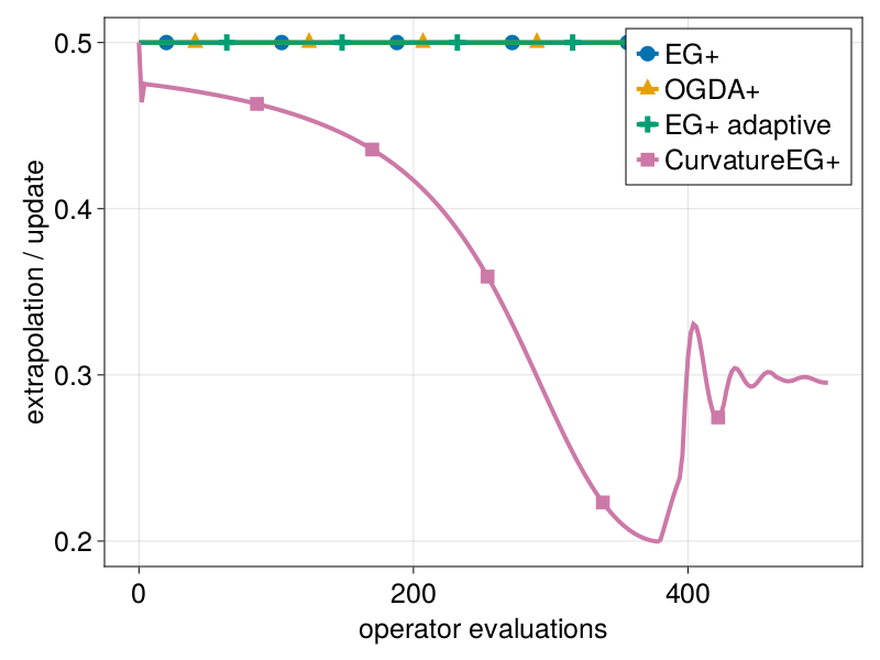
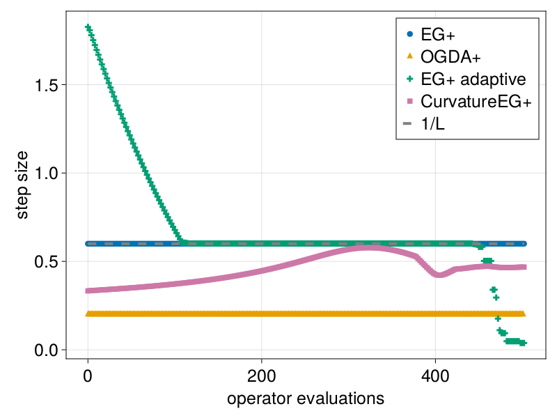
Refer to caption
(a) Ratio of extrapolation to update step
Refer to caption
(b) Extrapolation step size.
Figure 5: Ratio game. An illustration of the step sizes used by different methods, as well as the ratio of extrapolation to update step. CurvatureEG++ chooses its own ratio adaptively and does so for this example in a seemingly overly conservative way, resulting in slow convergence observed in FigureΒ 3.

C.1.1 Polar Game

For FigureΒ 2 we used the so-called Polar Game introduced inΒ [44] which is given by

F​(x,y)=(Οˆβ€‹(x,y)βˆ’y,Οˆβ€‹(y,x)+x),𝐹π‘₯π‘¦πœ“π‘₯π‘¦π‘¦πœ“π‘¦π‘₯π‘₯F(x,y)=(\psi(x,y)-y,\psi(y,x)+x), (30)

where Οˆβ€‹(x,y)=116​a​x​(βˆ’1+x2+y2)​(βˆ’9+16​x2+16​y2)πœ“π‘₯𝑦116π‘Žπ‘₯1superscriptπ‘₯2superscript𝑦2916superscriptπ‘₯216superscript𝑦2\psi(x,y)=\frac{1}{16}ax(-1+x^{2}+y^{2})(-9+16x^{2}+16y^{2}) and parameter a>0π‘Ž0a>0. In FigureΒ 2 we used a=13π‘Ž13a=\frac{1}{3}.