Wasserstein Iterative Networks
for Barycenter Estimation

Abstract

Wasserstein barycenters have become popular due to their ability to represent the average of probability measures in a geometrically meaningful way. In this paper, we present an algorithm to approximate the Wasserstein-2 barycenters of continuous measures via a generative model. Previous approaches rely on regularization (entropic/quadratic) which introduces bias or on input convex neural networks which are not expressive enough for large-scale tasks. In contrast, our algorithm does not introduce bias and allows using arbitrary neural networks. In addition, based on the celebrity faces dataset, we construct Ave, celeba! dataset which can be used for quantitative evaluation of barycenter algorithms by using standard metrics of generative models such as FID.

1 Introduction

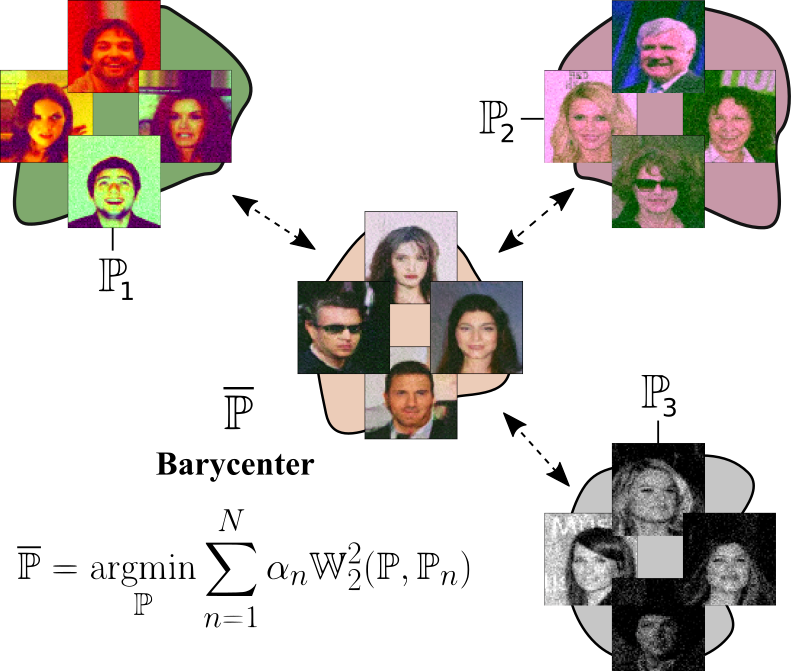
Figure 1: The barycenter w.r.t. weights ${(\alpha_{1},\alpha_{2},\alpha_{3})=(\frac{1}{4},\frac{1}{2},\frac{1}{4})}$ of Ave, Celeba! subsets computed by our Algorithm 1.
The figure shows random samples from the input subsets and generated images from the barycenter.

Wasserstein barycenters (agueh2011barycenters, ) provide a geometrically meaningful notion of the average of probability measures based on optimal transport (OT, see villani2008optimal ). Methods for computing barycenters have been successfully applied to various practical problems. In geometry processing, shape interpolation can be performed by barycenters (solomon2015convolutional, ). In image processing, barycenters are used for color and style translation (rabin2014adaptive, ; mroueh2019wasserstein, ), texture mixing (rabin2011wasserstein, ) and image interpolation (lacombe2021learning, ; simon2020barycenters, ). In language processing, barycenters can be applied to text evaluation (colombo2021automatic, ). In online learning, barycenters are used for aggregating probabilistic forecasts of experts (korotin2021mixability, ; paris2021online, ; koldasbayeva2022large, ). In Bayesian inference, the barycenter of subset posteriors converges to the full data posterior (srivastava2015wasp, ; srivastava2018scalable, ) allowing efficient computation of full posterior based on barycenters. In reinforcement learning, barycenters are used for uncertainty propagation (metelli2019propagating, ). Other applications are data augmentation (bespalov2021data, ), multivariate density registration (bigot2019data, ), distributions alignment (inouye2021iterative, ), domain generalization (lyu2021barycenteric, ) and adaptation montesuma2021wasserstein , model ensembling (dognin2019wasserstein, ), averaging of persistence diagrams vidal2019progressive ; barannikov2021manifold ; barannikov2021representation .

The bottleneck of obtaining barycenters is the computational complexity. For discrete measures, fast and accurate barycenter algorithms exist for low-dimensional problems; see peyre2019computational for a survey. However, discrete methods scale poorly with the number of support points of the barycenter. Consequently, they cannot approximate continuous barycenters well, especially in high dimensions.

Existing continuous barycenter approaches (li2020continuous, ; fan2020scalable, ; korotin2021continuous, ) are mostly based on entropic/quadratic regularization or parametrization of Brenier potentials with input-convex neural networks (ICNNs, see amos2017input ). The regularization-based $[\text{CR}\mathbb{W}\text{B}]$ algorithm by li2020continuous recovers a barycenter biased from the true one. Algorithms $[\text{C}\mathbb{W}_{2}\text{B}]$ by korotin2021continuous and $[\text{SC}\mathbb{W}_{2}\text{B}]$ by fan2020scalable based on ICNNs resolve this issue, see (korotin2021continuous, , Tables 1-3). However, despite the growing popularity of ICNNs in OT applications (makkuva2019optimal, ; korotin2019wasserstein, ; mokrov2021large, ), they could be suboptimal architectures according to a recent study (korotin2021neural, ). According to the authors, more expressive networks without the convexity constraint outperform ICNNs in practical OT problems.

Furthermore, evaluation of barycenter algorithms is challenging due to the limited number of continuous measures with explicitly known barycenters. It can be computed when the input measures are location-scatter (e.g. Gaussians) (alvarez2016fixed, , 4) or $1$-dimensional (bonneel2015sliced, , 2.3). Recent works (li2020continuous, ; korotin2021continuous, ; fan2020scalable, ) consider the Gaussian case in dimensions $\leq 256$ for quantitative evaluation. In higher dimensions, the computation of the ground truth barycenter is hard even for the Gaussian case: it involves matrix inversion and square root extraction (altschuler2021averaging, , Algorithm 1) with the cubic complexity in the dimension.

Contributions.

• We develop a novel iterative algorithm (4) for estimating Wasserstein-2 barycenters based on the fixed point approach by (alvarez2016fixed, ) combined with a neural solver for optimal transport (korotin2021neural, ). Unlike predecessors, our algorithm does not introduce bias and allows arbitrary network architectures.

• We construct the Ave, celeba! (averaging celebrity faces, 5) dataset consisting of $64\times 64$ RGB images for large-scale quantitative evaluation of continuous Wasserstein-2 barycenter algorithms. The dataset includes 3 subsets of degraded images of faces (Figure 1). The barycenter of these subsets corresponds to the original clean faces.

Our algorithm is suitable for large-scale Wasserstein-2 barycenters applications. The developed dataset will allow quantitative evaluation of barycenter algorithms at a large scale improving transparency and allowing healthy competition in the optimal transport research.

Notation. We work in a Euclidean space $\mathbb{R}^{D}$ for some $D$. All the integrals are computed over $\mathbb{R}^{D}$ unless stated otherwise. We denote the set of all Borel probability measures on $\mathbb{R}^{D}$ with finite second moment by $\mathcal{P}_{2}(\mathbb{R}^{D})$. We use $\mathcal{P}_{2,\text{ac}}(\mathbb{R}^{D})\subset\mathcal{P}_{2}(\mathbb{R}^{D})$ to denote the subset of absolutely continuous measures. We denote its subset of measures with positive density by $\mathcal{P}_{2,\text{ac}}^{+}(\mathbb{R}^{D})\subset\mathcal{P}_{2,\text{ac}}(\mathbb{R}^{D})$. We denote the set of probability measures on $\mathbb{R}^{D}\times\mathbb{R}^{D}$ with marginals $\mathbb{P}$ and $\mathbb{Q}$ by $\Pi(\mathbb{P},\mathbb{Q})$. For a measurable map $T:\mathbb{R}^{D}\rightarrow\mathbb{R}^{D}$, we denote the associated push-forward operator by $T\sharp$. For $\phi:\mathbb{R}^{D}\rightarrow\mathbb{R}$, we denote by $\overline{\phi}$ its Legendre-Fenchel transform (fenchel1949conjugate, ) defined by $\overline{\phi}(y)=\max_{x\in\mathbb{R}^{D}}[\langle x,y\rangle-\phi(x)]$. Recall that $\overline{\phi}$ is a convex function, even when $\phi$ is not.

2 Preliminaries

Wasserstein-2 distance. For ${\mathbb{P},\mathbb{Q}\!\in\!\mathcal{P}_{2}(\mathbb{R}^{D})}$, Monge’s primal formulation of the squared Wasserstein-2 distance, i.e., OT with quadratic cost, is

$$\mathbb{W}_{2}^{2}(\mathbb{P},\mathbb{Q})\stackrel{{\scriptstyle\text{def}}}{{=}}\min_{T\sharp\mathbb{P}=\mathbb{Q}}\ \int\frac{1}{2}\|x-T(x)\|^{2}d\mathbb{P}(x),$$ (1)

where the minimum is taken over measurable functions (transport maps) $T:\mathbb{R}^{D}\rightarrow\mathbb{R}^{D}$ mapping $\mathbb{P}$ to $\mathbb{Q}$. The optimal $T^{*}$ is called the optimal transport map. Note that (1) is not symmetric, and this formulation does not allow mass splitting. That is, for some ${\mathbb{P},\mathbb{Q}\in\mathcal{P}_{2}(\mathbb{R}^{D})}$, there might be no map $T$ that satisfies $T\sharp\mathbb{P}=\mathbb{Q}$. Thus, kantorovitch1958translocation proposed the following relaxation:

$$\mathbb{W}_{2}^{2}(\mathbb{P},\mathbb{Q})\stackrel{{\scriptstyle\text{def}}}{{=}}\min_{\pi\in\Pi(\mathbb{P},\mathbb{Q})}\int_{\mathbb{R}^{D}\times\mathbb{R}^{D}}\frac{1}{2}\|x-y\|^{2}d\pi(x,y),$$ (2)

where the minimum is taken over all transport plans $\pi$, i.e., measures on $\mathbb{R}^{D}\times\mathbb{R}^{D}$ whose marginals are $\mathbb{P}$ and $\mathbb{Q}$. The optimal $\pi^{*}\in\Pi(\mathbb{P},\mathbb{Q})$ is called the optimal transport plan. If $\pi^{*}$ is of the form $[\text{id},T^{*}]\sharp\mathbb{P}\in\Pi(\mathbb{P},\mathbb{Q})$ for some $T^{*}$, then $T^{*}$ minimizes (1). The dual form (villani2003topics, ) of $\mathbb{W}_{2}^{2}$ is:

$$\mathbb{W}_{2}^{2}(\mathbb{P},\mathbb{Q})\!=\!\max_{u\oplus v\leq\frac{\|\cdot\|^{2}}{2}}\bigg{[}\int u(x)d\mathbb{P}(x)+\int v(y)d\mathbb{Q}(y)\bigg{]},$$ (3)

where the maximum is taken over ${u\in\mathcal{L}^{1}(\mathbb{P})}$, ${v\in\mathcal{L}^{1}(\mathbb{Q})}$ satisfying ${u(x)+v(y)\!\leq\!\frac{1}{2}\|x-y\|^{2}}$ for all ${x,y\!\in\!\mathbb{R}^{D}}$. The functions $u$ and $v$ are called potentials. There exist optimal $u^{*},v^{*}$ satisfying $u^{*}=(v^{*})^{c}$, where ${f^{c}(y)\stackrel{{\scriptstyle def}}{{=}}\min\limits_{x\in\mathbb{R}^{D}}\big{[}\frac{1}{2}\|x-y\|^{2}-f(x)\big{]}}$ is the $c$-transform of $f$. We rewrite (3) as

$$\mathbb{W}_{2}^{2}(\mathbb{P},\mathbb{Q})=\max_{v}\bigg{[}\int v^{c}(x)d\mathbb{P}(x)+\int v(y)d\mathbb{Q}(y)\bigg{]},$$ (4)

where the maximum is taken over all $v\in\mathcal{L}^{1}(\mathbb{Q})$. It is customary (villani2008optimal, , Cases 5.3 & 5.17) to define ${u(x)\!=\!\frac{1}{2}\|x\|^{2}\!-\!\psi(x)}$ and ${v(y)\!=\!\frac{1}{2}\|y\|^{2}\!-\!\phi(x)}$. There exist convex optimal $\psi^{*}$ and $\phi^{*}$ satisfying $\overline{\psi^{*}}=\phi^{*}$ and $\overline{\phi^{*}}=\psi^{*}$. If $\mathbb{P}\in\mathcal{P}_{2,ac}(\mathbb{R}^{D})$, then the optimal $T^{*}$ of (1) always exists and can be recovered from the dual solution $u^{*}$ (or $\psi^{*}$) of (3): $T^{*}(x)=x-\nabla u^{*}(x)=\nabla\psi^{*}(x)$ (santambrogio2015optimal, , Theorem 1.17). The map $T^{*}$ is a gradient of a convex function, see the Brenier Theorem (brenier1991polar, ).

Wasserstein-2 barycenter. Let $\mathbb{P}_{1},\dots,\mathbb{P}_{N}\in\mathcal{P}_{2,ac}(\mathbb{R}^{D})$ such that at least one of them has bounded density. Their barycenter w.r.t. weights $\alpha_{1},\dots,\alpha_{N}$ ($\alpha_{n}\!>\!0$; ${\sum_{n=1}^{N}\alpha_{n}=1}$) is given by (agueh2011barycenters, ):

$$\overline{\mathbb{P}}\stackrel{{\scriptstyle\text{def}}}{{=}}\operatorname*{arg\,min}_{\mathbb{P}\in\mathcal{P}_{2}(\mathbb{R}^{D})}\sum_{n=1}^{N}\alpha_{n}\mathbb{W}_{2}^{2}(\mathbb{P}_{n},\mathbb{P}).$$ (5)

The barycenter $\overline{\mathbb{P}}$ exists uniquely and $\overline{\mathbb{P}}\in\mathcal{P}_{2,ac}(\mathbb{R}^{D})$. Moreover, its density is bounded (agueh2011barycenters, , Definition 3.6 & Theorem 5.1). For $n\in\{1,2,\dots,N\}$, let $T_{\overline{\mathbb{P}}\rightarrow\mathbb{P}_{n}}=\nabla\psi_{n}^{*}$ be the OT maps from $\overline{\mathbb{P}}$ to $\mathbb{P}_{n}$. The following holds $\overline{\mathbb{P}}$-almost everywhere:

$$\sum_{n=1}^{N}\alpha_{n}T_{\overline{\mathbb{P}}\rightarrow\mathbb{P}_{n}}(x)=\sum_{n=1}^{N}\alpha_{n}\nabla\psi^{*}_{n}(x)=x,$$ (6)

see (alvarez2016fixed, , 3). If $\overline{\mathbb{P}}\in\mathcal{P}_{2,\text{ac}}^{+}(\mathbb{R}^{D})$, then (6) holds for every $x\in\mathbb{R}^{D}$, i.e., $\sum_{n=1}^{N}\alpha_{n}\psi_{n}^{*}(x)=\frac{\|x\|^{2}}{2}+c$. We call such convex potentials $\psi_{n}^{*}$ congruent.

3 Related Work

Below we review existing continuous methods for OT. In 3.1, we discuss methods for OT problems (1), (2), (3). In 3.2, we review algorithms that compute barycenters (5).

3.1 Continuous OT Solvers for $\mathbb{W}_{2}$

We use the phrase OT solver to denote any method capable of recovering $T^{*}$ or $u^{*}$ (or $\psi^{*}$).

Primal-form solvers based on (1) or (2), e.g., xie2019scalable ; lu2020large , parameterize $T^{*}$ using complicated generative modeling techniques with adversarial losses to handle the pushforward constraint $T\sharp\mathbb{P}=\mathbb{Q}$ in the primal form (1). They depend on careful hyperparameter search and complex optimization (lucic2018gans, ).

Dual-form continuous solvers (genevay2016stochastic, ; seguy2017large, ; nhan2019threeplayer, ; taghvaei20192, ; korotin2019wasserstein, ) based on (3) or (4) have straightforward optimization procedures and can be adapted to various tasks without extensive hyperparameter search.

A comprehensive overview and a benchmark of dual-form solvers are given in korotin2021neural . According to the evaluation, the best performing OT solver is reversed maximin solver $\lfloor\text{MM:R}\rceil$, a modification of the idea proposed by nhan2019threeplayer in the context of Wasserstein-1 GANs (arjovsky2017wasserstein, ). In this paper, we employ this solver as a part of our algorithm. We review it below.

Reversed Maximin Solver. In (4), $v^{c}(x)$ can be expanded through $v$ via the definition of $c$-transform:

$$\max_{v}\!\int\!\min_{y\in\mathbb{R}^{D}}\big{[}\frac{\|x-y\|^{2}_{2}}{2}-v(y)\big{]}d\mathbb{P}(x)\!+\!\int v(y)d\mathbb{Q}(y)\!=$$

$$\max_{v}\min_{T}\!\int\bigg{[}\frac{\|x\!-\!T(x)\|^{2}_{2}}{2}\!-\!v\big{(}T(x)\big{)}\!\bigg{]}\!d\mathbb{P}(x)\!+\int v(y)d\mathbb{Q}(y).$$ (7)

In (7), the optimization over ${y\in\mathbb{R}^{D}}$ is replaced by the equivalent optimization over functions ${T:\mathbb{R}^{D}\rightarrow\mathbb{R}^{D}}$. This is done by the interchanging of integral and minimum, see (rockafellar1976integral, , Theorem 3A).

The key point of this reformulation is that the optimal solution of this maximin problem is given by $(v^{*},T^{*})$, where $T^{*}$ is the OT map from $\mathbb{P}$ to $\mathbb{Q}$, see discussion in (korotin2021neural, , 2) or (rout2021generative, , 4.1). In practice, the potential $v:\mathbb{R}^{D}\rightarrow\mathbb{R}$ and the map ${T:\mathbb{R}^{D}\rightarrow\mathbb{R}^{D}}$ are parametrized by neural networks $v_{\omega},T_{\theta}$. To train $\theta$ and $\omega$, stochastic gradient ascent/descent (SGAD) over mini-batches from $\mathbb{P},\mathbb{Q}$ is used.

3.2 Algorithms for Continuous $\mathbb{W}_{2}$ Barycenters

Variational optimization. Problem (5) is optimization over probability measures. To estimate $\overline{\mathbb{P}}$, one may employ a generator $G_{\xi}:\mathbb{R}^{H}\rightarrow\mathbb{R}^{D}$ with a latent measure $\mathbb{S}$ on $\mathbb{R}^{H}$ and train $\xi$ by minimizing

$$\sum_{n=1}^{N}\alpha_{n}\mathbb{W}_{2}^{2}(\underbrace{G_{\xi}\sharp\mathbb{S}}_{\mathbb{P}_{\xi}},\mathbb{P}_{n})\rightarrow\min_{\xi}\!.$$ (8)

Optimization (8) can be performed by using SGD on random mini-batches from measures $\mathbb{P}_{n}$ and $\mathbb{S}$. The difference between possible variational algorithms lies in the particular estimation method for $\mathbb{W}_{2}^{2}$ terms. To our knowledge, only ICNN-based minimax solver (makkuva2019optimal, ) has been used to compute $\mathbb{W}_{2}^{2}$ in (8) yielding $[\text{SC}\mathbb{W}_{2}\text{B}]$ algorithm (fan2020scalable, ).

Potential-based optimization. li2020continuous ; korotin2021continuous recover the optimal potentials $\{\psi^{*}_{n},\phi^{*}_{n}\}$ for each pair $(\overline{\mathbb{P}},\mathbb{P}_{n})$ via a non-minimax regularized dual formulation. No generative model is needed: the barycenter is recovered by pushing forward measures using gradients of potentials or by barycentric projection. However, the non-trivial choice of the prior barycenter distribution is required. Algorithm $[\text{CR}\mathbb{W}\text{B}]$ by li2020continuous use entropic or quadratic regularization and $[\text{C}\mathbb{W}_{2}\text{B}]$ algorithm by korotin2021continuous uses ICNNs, congruence and cycle-consistency (korotin2019wasserstein, ) regularization.

Other methods. Recent work chi2021variational combines the variational (8) and potential-based optimization via the $c$-cyclical monotonity regularization. In daaloul2021sampling , an algorithm to sample from the continuous Wasserstein barycenter via the gradient flows is proposed.

4 Iterative $\mathbb{W}_{2}$-Barycenter Algorithm

Our proposed algorithm is based on the fixed point approach by alvarez2016fixed which we recall in 4.1. In 4.2, we formulate our algorithm for computing Wasserstein-2 barycenters. In 4.3, we show that our algorithm generalizes the variational barycenter approach.

4.1 Theoretical Fixed Point Approach

Following alvarez2016fixed , we define an operator $\mathcal{H}:\mathcal{P}_{2,ac}(\mathbb{R}^{D})\!\rightarrow\!\mathcal{P}_{2,ac}(\mathbb{R}^{D})$ by ${\mathcal{H}(\mathbb{P})=[\sum_{n=1}^{N}\alpha_{n}T_{\mathbb{P}\rightarrow\mathbb{P}_{n}}]\sharp\mathbb{P},}$ where $T_{\mathbb{P}\rightarrow\mathbb{P}_{n}}$ denotes the OT map from $\mathbb{P}$ to $\mathbb{P}_{n}$. The measure $\mathcal{H}(\mathbb{P})$ obtained by the operator is indeed absolutely continuous, see (alvarez2016fixed, , Theorem 3.1). According to (6), the barycenter $\overline{\mathbb{P}}$ defined by (5) is a fixed point of $\mathcal{H}$, i.e., $\mathcal{H}(\overline{\mathbb{P}})=\overline{\mathbb{P}}$. This suggests a way to compute $\overline{\mathbb{P}}$ by picking some ${\mathbb{P}\in\mathcal{P}_{2,ac}(\mathbb{R}^{D})}$ and recursively applying $\mathcal{H}$ until convergence. However, there are several challenges:

1. A fixed point $\mathbb{P}\in\mathcal{P}_{2,\text{ac}}(\mathbb{R}^{D})$ satisfying $\mathcal{H}(\mathbb{P})=\mathbb{P}$ may be not the barycenter (alvarez2016fixed, , Example 3.1). The situation is analogous to that of the iterative $k$-means algorithm for a different problem – clustering. There may be fixed points which are not globally optimal.

2. The sequence $\{\mathcal{H}^{k}(\mathbb{P})\}_{k}$ is tight (alvarez2016fixed, , Theorem 3.6) so it has a subsequence converging in $\mathcal{P}_{2,ac}(\mathbb{R}^{D})$, but the entire sequence may not converge. Nevertheless, the value of the objective (5) decreases for $\mathcal{H}^{k}(\mathbb{P})$ as $k\rightarrow\infty$ (alvarez2016fixed, , Prop. 3.3).

3. Efficient parametrization of the evolving measure $\mathcal{H}^{k}(\mathbb{P})$ is required. Moreover, to get $\mathcal{H}^{k+1}(\mathbb{P})$ from $\mathcal{H}^{k}(\mathbb{P})$, one needs to compute $N$ optimal transport maps $T_{\mathcal{H}^{k}(\mathbb{P})\rightarrow\mathbb{P}_{n}}$ which can be costly.

In chewi2020gradient and altschuler2021averaging , the fixed point approach is considered in the Gaussian case where the sequence $\mathcal{H}^{k}(\mathbb{P})$ is guaranteed to converge to the unique fixed point – the barycenter. The Gaussian case also makes parameterization (c) simple since both measures $\mathbb{P}_{n}$ and $\mathcal{H}^{k}(\mathbb{P})$ can be parametrized by means and covariance matrices, and the maps $T_{\mathcal{H}^{k}(\mathbb{P})\rightarrow\mathbb{P}_{n}}$ are linear with closed form.

For general continuous measures $\mathbb{P}_{n}$, it remains an open problem to find sharp conditions on inputs $\mathbb{P}_{n}$ and the initial measure $\mathbb{P}$ of the fixed-point iteration for the sequence $\{\mathcal{H}^{k}(\mathbb{P})\}_{k}$ to converge to the barycenter. In this work, we empirically verify that the fixed point approach works well for the input measures that we consider and for a randomly initialized generative model representing the evolving barycenter (4.2). We tackle challenge (c) and develop a scalable optimization procedure that requires only sample access to ${\mathbb{P}_{n}\!\in\!\mathcal{P}_{2,ac}(\mathbb{R}^{D})}$.

4.2 Practical Iterative Optimization Procedure

We employ a generative model to parametrize the evolving measure, i.e., put ${\mathbb{P}_{\xi}=G_{\xi}\sharp\mathbb{S}}$, where $\mathbb{S}$ is a latent measure, e.g., $\mathbb{S}=\mathcal{N}(0,I_{H})$, and $G_{\xi}$ is a neural network $\mathbb{R}^{H}\rightarrow\mathbb{R}^{D}$ with parameters $\xi$. Our approach to compute the operator $\mathcal{H}(\mathbb{P}_{\xi})$ and update $G_{\xi}$ consists of two steps.

First, we approximately recover $N$ maps $T_{\mathbb{P}_{\xi}\rightarrow\mathbb{P}_{n}}$ via $\lceil\text{MM:R}\rfloor$ solver, i.e., we use $N$ pairs or networks $\{T_{\theta_{n}},v_{\omega_{n}}\}$ and train them by optimizing (7) with ${\mathbb{P}\leftarrow\mathbb{P}_{\xi}}$ and ${\mathbb{Q}\leftarrow\mathbb{P}_{n}}$. For each $n=1,2,\dots,N$, we perform SGAD by using batches from $G_{\xi}\sharp\mathbb{S}$ and $\mathbb{P}_{n}$ and get $T_{\theta_{n}}\approx T_{\mathbb{P}_{\xi}\rightarrow\mathbb{P}^{n}}$.

Second, we update $G_{\xi}$ to represent $\mathcal{H}(\mathbb{P}_{\xi})$ instead of $\mathbb{P}_{\xi}$. Inspired by chen2019gradual , we do this via regression. We introduce $G_{\xi_{0}}$, a fixed copy of $G_{\xi}$. Next, we regress $G_{\xi}(\cdot)$ onto $\sum_{n=1}^{N}\alpha_{n}T_{\theta_{n}}\big{(}G_{\xi_{0}}(\cdot)\big{)}$

$$\int_{z}\boldsymbol{\ell}\bigg{(}G_{\xi}(z),\sum_{n=1}^{N}\alpha_{n}T_{\theta_{n}}\big{(}G_{\xi_{0}}(z)\big{)}\bigg{)}d\mathbb{S}(z)\rightarrow\min_{\xi}$$

by performing SGD on random batches from $\mathbb{S}$, e.g., by using squared error ${\boldsymbol{\ell}(x,x^{\prime})\!\stackrel{{\scriptstyle\text{def}}}{{=}}\!\frac{1}{2}\|x-x^{\prime}\|^{2}}$. Thus, generator $G_{\xi}(\cdot)$ becomes close to ${\sum_{n=1}^{N}\!\alpha_{n}T_{\theta_{n}}\big{(}G_{\xi_{0}}(\cdot)\big{)}}$ as a function $\mathbb{R}^{H}\!\rightarrow\!\mathbb{R}^{D}$. We get

$$\mathbb{P}_{\xi}=G_{\xi}\sharp\mathbb{S}\approx\big{[}\sum_{n=1}^{N}\alpha_{n}T_{\theta_{n}}\big{]}\sharp\big{[}G_{\xi_{0}}\sharp\mathbb{S}\big{]}=\big{[}\sum_{n=1}^{N}\alpha_{n}T_{\theta_{n}}\big{]}\sharp\mathbb{P}_{\xi_{0}}\approx\big{[}\sum_{n=1}^{N}\alpha_{n}T_{\mathbb{P}_{\xi_{0}}\rightarrow\mathbb{P}_{n}}\big{]}\sharp\mathbb{P}_{\xi_{0}}=\mathcal{H}(\mathbb{P}_{\xi_{0}}),$$

i.e., the new generated $G_{\xi}\sharp\mathbb{S}$ measure approximates $\mathcal{H}(\mathbb{P}_{\xi_{0}})$.

Summary. Our two-step approach iteratively recomputes OT maps $T_{\mathbb{P}_{\xi}\rightarrow\mathbb{P}_{n}}$ (Figure 2(a)) and then uses regression to update the generator (Figure 2(b)). The optimization procedure is detailed in Algorithm 1. Note that when fitting OT maps $T_{\mathbb{P}_{\xi}\rightarrow\mathbb{P}^{n}}$, we start from previously used $\{T_{\theta_{n}},v_{\omega_{n}}\}$ rather than re-initialize them. Empirically, this works better.

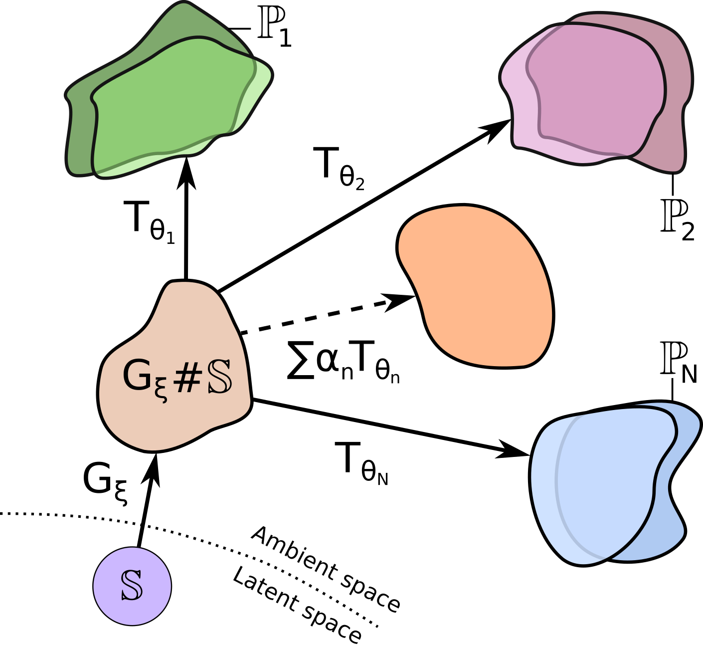
(a) Step 1. We compute $N$ approximate OT maps $T_{\theta_{n}}$ from generated measure $\mathbb{P}_{\xi}=G_{\xi}\sharp\mathbb{S}$ to input measures $\mathbb{P}_{n}$.

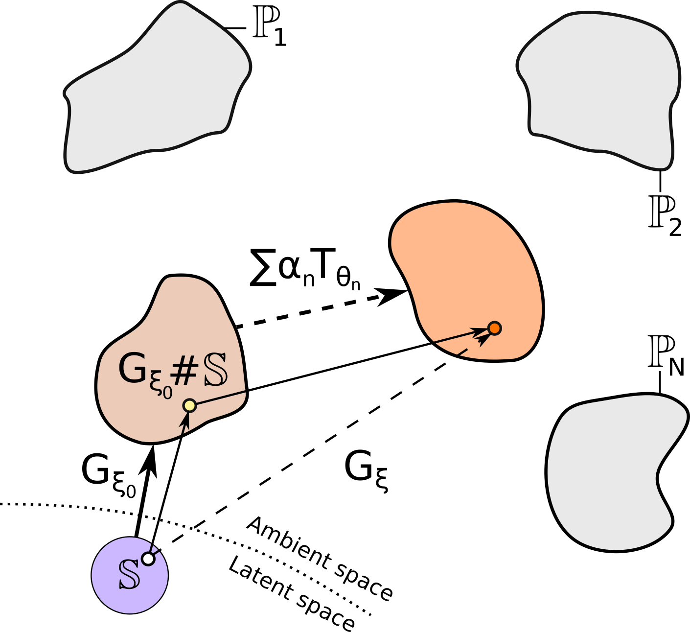
(b) Step 2. We regress $G_{\xi}(\cdot)$ onto $\sum_{n=1}^{N}\alpha_{n}T_{\theta_{n}}\big{(}G_{\xi_{0}}(\cdot)\big{)}$, where $G_{\xi_{0}}$is a fixed copy of $G_{\xi}$ before the update.

Figure 2: Our proposed two-step implementation of the fixed-point operator $\mathcal{H}(\cdot)$..

 

4.3 Relation to Variational Barycenter Algorithms

We show that our Algorithm 1 reduces to variational approach (3.2) when the number of generator updates, $K_{G}$, is equal to $1$. More specifically, we show the equivalence of the gradient update w.r.t. parameters $\xi$ of the generator in our iterative Algorithm 1 and that of (8). We assume that $\mathbb{W}_{2}^{2}$ terms are computed exactly in (8) regardless of the particular OT solver. Similarly, in Algorithm 1, we assume that maps $G_{\xi_{0}}\sharp\mathbb{S}\rightarrow\mathbb{P}_{n}$ before the generator update are always exact, i.e., $T_{\theta_{n}}=T_{\mathbb{P}_{\xi_{0}}\rightarrow\mathbb{P}_{n}}$.

Lemma 1.

Assume that $\mathbb{P}_{\xi}\!=\!G_{\xi}\sharp\mathbb{S}\!\in\!\mathcal{P}_{2,ac}(\mathbb{R}^{D})$. Consider $K_{G}=1$ for the iterative Algorithm 1, i.e., we do a single gradient step regression update per OT solvers’ update. Assume that $\boldsymbol{\ell}(x,x^{\prime})=\frac{1}{2}\|x-x^{\prime}\|^{2}$, i.e., the squared loss is used for regression. Then the generator’s gradient update in Algorithm 1 is the same as in the variational algorithm:

$$\frac{\partial}{\partial\xi}\int_{z}\frac{1}{2}\big{\lVert}G_{\xi}(z)\!-\!\sum_{n=1}^{N}\alpha_{n}T_{\mathbb{P}_{\xi_{0}}\rightarrow\mathbb{P}_{n}}\big{(}G_{\xi_{0}}(z)\big{)}\big{\rVert}^{2}d\mathbb{S}(z)=\frac{\partial}{\partial\xi}\sum_{n=1}^{N}\alpha_{n}\mathbb{W}_{2}^{2}(G_{\xi}\sharp\mathbb{S},\mathbb{P}_{n}),$$ (9)

where the derivatives are evaluated at $\xi=\xi_{0}$.

We prove the lemma in Appendix A. In practice, we choose $K_{G}=50$ as it empirically works better.

Input : latent $\mathbb{S}$ and input $\mathbb{P}_{1},\dots,\mathbb{P}_{N}$ measures; weights $\alpha_{1},\dots,\alpha_{N}>0$ ($\sum_{n=1}^{N}\alpha_{n}=1$); number of iters per network: $K_{G}$, $K_{T}$, $K_{v}$; generator $G_{\xi}:\mathbb{R}^{H}\rightarrow\mathbb{R}^{D}$;

mapping networks $T_{\theta_{1}},\dots,T_{\theta_{N}}:\mathbb{R}^{D}\rightarrow\mathbb{R}^{D}$; potentials $v_{\omega_{1}},\dots,v_{\omega_{N}}:\mathbb{R}^{D}\rightarrow\mathbb{R}$;

regression loss $\boldsymbol{\ell}:\mathbb{R}^{D}\times\mathbb{R}^{D}\rightarrow\mathbb{R}_{+}$;

Output : generator satisfying $G_{\xi}\sharp\mathbb{S}\approx\overline{\mathbb{P}}$; OT maps satisfying $T_{\theta_{n}}\sharp(G_{\xi}\sharp\mathbb{S})\approx\mathbb{P}_{n}$;

repeat

     # OT solvers update

     for $n=1,2,\dots,N$ do

         for $k_{v}=1,2,\dots,K_{v}$ do

             Sample batches $Z\!\sim\!\mathbb{S}$, $Y\!\sim\!\mathbb{P}_{n}$; $X\!\leftarrow\!G_{\xi}(Z)$;

             $\mathcal{L}_{v}\leftarrow\frac{1}{|X|}\sum\limits_{x\in X}v_{\omega_{n}}\big{(}T_{\theta_{n}}(x)\big{)}-\frac{1}{|Y|}\sum\limits_{y\in Y}v_{\omega_{n}}\big{(}y\big{)}$;

             Update $\omega_{n}$ by using $\frac{\partial\mathcal{L}_{v}}{\partial\omega_{n}}$;

            

            for $k_{T}=1,2,\dots,K_{T}$ do

                 Sample batch $Z\sim\mathbb{S}$; $X\leftarrow G_{\xi}(Z)$;

                 ${\mathcal{L}_{T}\!=\!\frac{1}{|X|}\!\sum\limits_{x\in X}\!\big{[}\frac{1}{2}\|x\!-\!T_{\theta_{n}}(x)\|^{2}\!-\!v_{\omega_{n}}\!\big{(}T_{\theta_{n}}(x)\big{)}\!\big{]}}$;

                 Update $\theta_{n}$ by using $\frac{\partial\mathcal{L}_{T}}{\partial\theta_{n}}$;

                

            

        

    

    # Generator update (regression)

     $G_{\xi_{0}}\leftarrow\text{copy}\big{(}G_{\xi}\big{)}$;

     for $k_{G}=1,2,\dots,K_{G}$ do

         Sample batch $Z\sim\mathbb{S}$;

         ${\mathcal{L}_{G}\!\leftarrow\!\frac{1}{|Z|}\!\sum\limits_{z\in Z}\boldsymbol{\ell}\bigg{(}G_{\xi}(z),\sum_{n=1}^{N}\alpha_{n}T_{\theta_{n}}\big{(}G_{\xi_{0}}(z)\big{)}\bigg{)}}$;

         Update $\xi$ by using $\frac{\partial\mathcal{L}_{G}}{\partial\xi}$;

        

    

until not converged;

Algorithm 1 Wasserstein Iterative Networks (WIN) for Barycenter Estimation

5 Ave, celeba! Images Dataset

In this section, we develop a generic methodology for building measures with known $\mathbb{W}_{2}$ barycenter. We then use it to construct Ave, celeba! dataset for quantitative evaluation of barycenter algorithms.

Key idea. Consider $\alpha_{1},\dots,\alpha_{N}>0$ with ${\sum_{n=1}^{N}\alpha_{n}=1}$, congruent convex functions ${\psi_{1},\dots\psi_{N}}:\mathbb{R}^{D}\rightarrow\mathbb{R}$, and a measure $\mathbb{P}\in\mathcal{P}_{2,\text{ac}}^{+}(\mathbb{R}^{D})$ with positive density. Define ${\mathbb{P}_{n}=\nabla\psi_{n}\sharp\mathbb{P}}$. Thanks to Brenier’s theorem brenier1991polar , $\nabla\psi_{n}$ is the unique OT map from $\mathbb{P}$ to $\mathbb{P}_{n}$. Since the support of $\mathbb{P}$ is $\mathbb{R}^{D}$, $\psi_{n}$ is the unique (up to a constant) dual potential for $(\mathbb{P},\mathbb{P}_{n})$ staudt2022uniqueness . Since potentials $\psi_{n}$’s are congruent, the barycenter $\overline{\mathbb{P}}$ of $\mathbb{P}_{n}$ w.r.t. weights $\alpha_{1},\dots,\alpha_{N}$ is $\mathbb{P}$ itself (chewi2020gradient, , C.2). If $\psi_{n}$’s are such that all $\mathbb{P}_{n}$ are absolutely continuous, then $\mathbb{P}=\overline{\mathbb{P}}$ is the unique barycenter (2).

If one obtains $N$ congruent $\psi_{n}$, then for any $\mathbb{P}\in\mathcal{P}_{2,ac}(\mathbb{R}^{D})$, pushforward measures ${\mathbb{P}_{n}=\nabla\psi_{n}\sharp\mathbb{P}}$ can be used as the input measures for the barycenter task. For $\mathbb{P}$ accessible by samples, measures $\mathbb{P}_{n}$ are also accessible by samples: one may sample $x\sim\mathbb{P}$ and push samples forward by $\nabla\psi_{n}$.

The challenging part is to construct non-trivial congruent convex functions $\psi_{n}$. First, we provide a novel method to transform a single convex function $\psi$ into a pair $(\psi^{l},\psi^{r})$ of convex functions satisfying $\alpha\nabla\psi^{l}(x)+(1-\alpha)\nabla\psi^{r}(x)=x$ for all $x\in\mathbb{R}^{D}$ (Lemma 2). Next, we extend the method to generate congruent $N$-tuples (Lemma 3).

Lemma 2 (Constructing congruent pairs).

Let $\psi$ be a strongly convex and $L$-smooth (for some $L>0$) function. Let $\beta\in(0,1)$. Define $\beta$-left and $\beta$-right functions of $\psi$ by

$$\psi^{l}\stackrel{{\scriptstyle\text{def}}}{{=}}\overline{\beta\frac{\|\cdot\|^{2}}{2}+(1-\beta)\psi}\qquad\text{and}\qquad\psi^{r}\stackrel{{\scriptstyle\text{def}}}{{=}}\overline{(1-\beta)\frac{\|\cdot\|^{2}}{2}+\beta\overline{\psi}}.$$ (10)

Then $\beta\psi^{l}(x)+(1-\beta)\psi^{r}(x)=\frac{\|x\|^{2}}{2}$ for $x\in\mathbb{R}^{D}$, i.e., convex functions $\psi^{l},\psi^{r}$ are congruent w.r.t. weights ${(\beta,1-\beta)}$. Besides, for all $x\in\mathbb{R}^{D}$ the gradient $y^{l}\stackrel{{\scriptstyle\text{def}}}{{=}}\nabla\psi^{l}(x)$ can be computed via solving $\beta$-strongly concave optimization:

$$y^{l}=\operatorname*{arg\,max}_{y\in\mathbb{R}}\bigg{(}\langle x,y\rangle-\beta\frac{\|y\|^{2}}{2}-(1-\beta)\psi(y)\bigg{)}.$$ (11)

In turn, the value $y^{r}\stackrel{{\scriptstyle\text{def}}}{{=}}\nabla\psi^{r}(x)$ is given by $y^{r}=\nabla\psi(y^{l})$.

The proof is given in Appendix A. We visualize the idea of our Lemma 2 in Figure 3(a). Thanks to Lemma 2, any analytically known convex $\psi$, e.g., an ICNN, can be used to produce a congruent pair $\psi^{l}$, $\psi^{r}$. To compute the gradient maps, optimization (11) can be solved by convex optimization tools with $\nabla\psi$ computed by automatic differentiation.

Lemma 3 (Constructing $N$ congruent functions.).

Let $\psi_{1}^{0},\dots,\psi_{M}^{0}$ be convex functions, $\beta_{1},\dots,\beta_{M}\in(0,1)$ and $\psi^{l}_{m},\psi^{r}_{m}$ be $\beta_{m}$-left, $\beta_{m}$-right functions for $\psi_{m}^{0}$ respectively. Let $\gamma^{l},\gamma^{r}\in\mathbb{R}^{N\times M}$ be two rectangular matrices with non-negative elements and the sum of elements in each column equals to $1$. Let $w_{1},\dots,w_{M}>0$ satisfy $\sum_{m=1}^{M}w_{m}=1$. For $n=1,\dots,N$ define

$$\psi_{n}(x)\!\stackrel{{\scriptstyle\text{def}}}{{=}}\!\frac{\sum_{m=1}^{M}\!w_{m}\big{[}\beta_{m}\gamma^{l}_{nm}\psi_{m}^{l}(x)\!+\!(1\!-\!\beta_{m})\gamma^{r}_{nm}\psi_{m}^{r}(x)\big{]}}{\sum_{m=1}^{M}\!w_{m}\big{[}\beta_{m}\gamma^{l}_{nm}\!+\!(1\!-\!\beta_{m})\gamma^{r}_{nm}\big{]}}.$$ (12)

Then $\psi_{1},\dots,\psi_{N}$ are congruent w.r.t. weights $\alpha_{n}\stackrel{{\scriptstyle\text{def}}}{{=}}\sum_{m=1}^{M}w_{m}\big{[}\beta_{m}\gamma^{l}_{nm}+(1-\beta_{m})\gamma^{r}_{nm}\big{]}.$

We prove Lemma 3 in Appendix A. We visualize the idea of our Lemma 3 in Figure 3(b). The lemma provides an elegant way to create $N\geq 2$ congruent functions from convex linear combinations of functions in given congruent pairs $(\psi_{m}^{l},\psi_{m}^{r})$. Gradients $\nabla\psi_{n}$ of these functions are respective linear combinations of gradients $\nabla\psi_{m}^{l}$ and $\nabla\psi_{m}^{r}$.

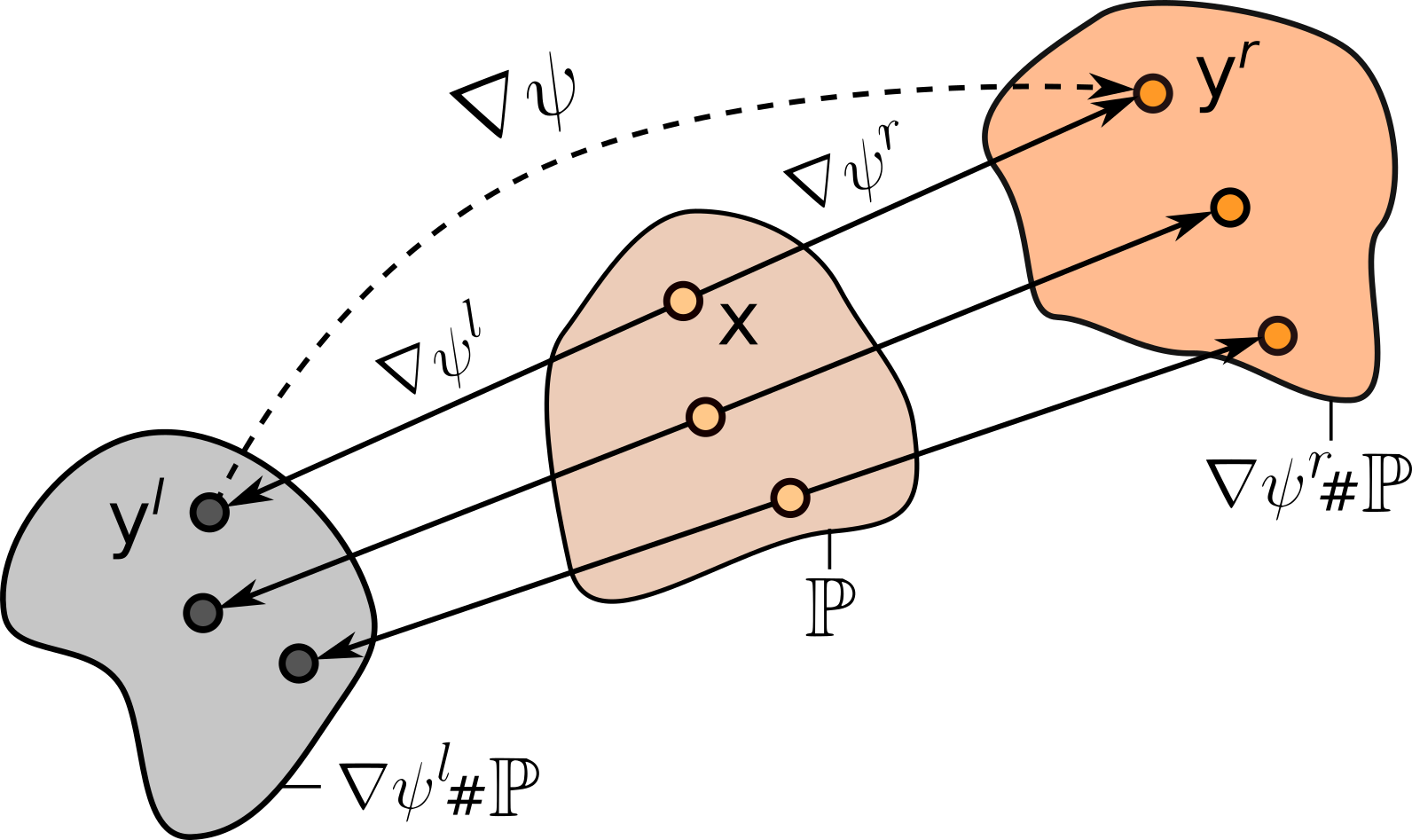
(a) Construction of a pair of congruent functions $\psi^{l},\psi^{r}$ from a convex $\psi$, see Lemma 2.

Figure 3: Construction of tuples of congruent functionsand production of measures with known $\mathbb{W}_{2}$ barycenter (5).

 

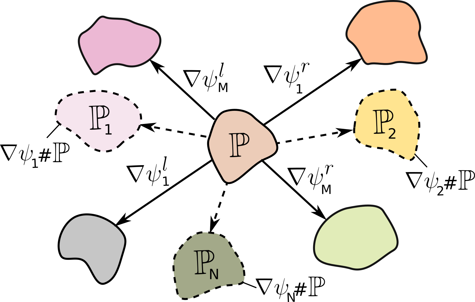
(b) Construction of $N$ congruent $\psi_{n}$ as convex combinations of $M$ congruent pairs $(\psi_{m}^{l},\psi_{m}^{r})$, see Lemma 3.

Dataset creation. We use CelebA $64\times 64$ faces dataset (liu2015faceattributes, ) as the basis for our Ave, celeba! dataset. We assume that CelebA dataset is an empirical sample from the continuous measure ${\mathbb{P}_{\text{Celeba}}\in\mathcal{P}_{2,\text{ac}}^{+}(\mathbb{R}^{3\times 64\times 64})}$ which we put to be the barycenter in our design, i.e., ${\overline{\mathbb{P}}=\mathbb{P}_{\text{Celeba}}}$. We construct diffirentiable congruent $\psi_{n}$ with bijective gradients that produce ${\mathbb{P}_{n}=\nabla\psi_{n}\sharp\overline{\mathbb{P}}\in\mathcal{P}_{2,\text{ac}}^{+}(\mathbb{R}^{3\times 64\times 64})}$ whose unique barycenter is $\mathbb{P}_{\text{Celeba}}$. In Lemma 3, we set $N=3$, $M=2$, $\beta_{1}=\beta_{2}=\frac{1}{2}$, $w_{1}=w_{2}=\frac{1}{2}$ and

$$(\gamma^{l})^{\top}=\begin{pmatrix}1&0&0\\ 0&1&0\end{pmatrix},\qquad(\gamma^{r})^{\top}=\begin{pmatrix}0&1&0\\ 0&0&1\end{pmatrix}\vspace{-0.3mm}\vspace{-2mm}$$

which yields weights $(\alpha_{1},\alpha_{2},\alpha_{3})=(\frac{1}{4},\frac{1}{2},\frac{1}{4})$ We choose the constants above manually to make sure the final produced measures $\mathbb{P}_{n}$ are visually distinguishable. We use $\psi_{m}^{0}(x)=\text{ICNN}_{m}\big{(}s_{m}(\sigma_{m}(d_{m}(x)))\big{)}+\lambda\frac{\|x\|^{2}}{2}$ as convex functions, where ICNNs have ConvICNN64 architecture (korotin2021neural, , Appendix B.1), $\sigma_{1},\sigma_{2}$ are random permutations of pixels and channels, $s_{1},s_{2}$ are axis-wise random reflections, $\lambda=\frac{1}{100}$. In both functions, $d_{m}$ is a de-colorization transform which sets R, G, B channels of each pixel to $(\frac{7}{10}\text{R}\!+\!\frac{1}{25}\text{G}\!+\!\frac{13}{50}\text{B})$ for $\psi_{1}^{0}$ and $\frac{1}{3}(\text{R}\!+\!\text{G}\!+\!\text{B})$ for $\psi_{2}^{0}$. The weights of ICNNs are initialized by the pre-trained potentials of $\mathbb{W}_{2}^{2}$ ”Early” transport benchmark which map blurry faces to the clean ones (korotin2021neural, , 4.1). All the implementation details are given in Appendix B.1.

Finally, to create Ave, celeba! dataset, we randomly split the images dataset into 3 equal parts containing $\approx 67$K samples, and map each part to respective measure ${\mathbb{P}_{n}=\nabla\psi_{n}\sharp\mathbb{P}_{\text{Celeba}}}$ by $\nabla\psi_{n}$. Resulting $3\times 67$K samples form the dataset consisting of $3$ parts. We show the samples in Figure 4. The samples from the respective parts are in green boxes.

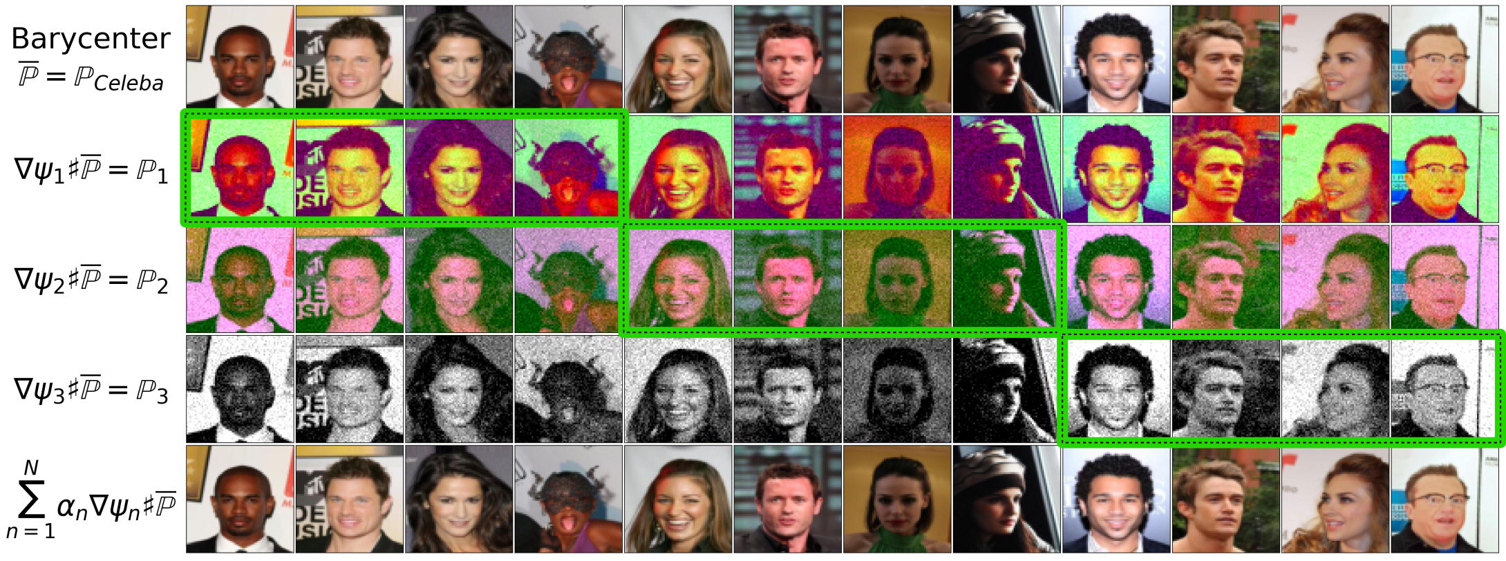
Figure 4: The production of Ave, celeba! dataset. The 1st line shows images ${x\sim\mathbb{P}_{\text{Celeba}}}$. Each of 3 next lines shows OT maps ${\nabla\psi_{n}(x)\sim\nabla\psi_{n}\sharp\mathbb{P}_{\text{Celeba}}=\mathbb{P}_{n}}$ to constructed measures $\mathbb{P}_{n}$. Their barycenter w.r.t. $(\alpha_{1},\alpha_{2},\alpha_{3})=(\frac{1}{4},\frac{1}{2},\frac{1}{4})$ is $\mathbb{P}_{\text{Celeba}}$. The last line shows congruence of $\psi_{n}$, i.e., ${\sum_{n=1}^{N}\alpha_{n}\nabla\psi_{n}(x)\equiv x}$. Samples in green boxes are included to dataset.

6 Evaluation

The code is written on the PyTorch and includes the script for producing Ave, celeba! dataset. The experiments are conducted on 4$\times$GPU GTX 1080ti. The details are given in Appendix B.

6.1 Evaluation on Ave, celeba! Dataset

We evaluate our iterative algorithm 1 and a recent state-of-the-art variational $[\text{SC}\mathbb{W}_{2}\text{B}]$ by fan2020scalable on Ave, celeba! dataset. Both algorithms use a generative model $\mathbb{P}_{\xi}=G_{\xi}\sharp\mathbb{S}$ for the barycenter and yield approximate maps $\widehat{T}_{\mathbb{P}_{\xi}\rightarrow\mathbb{P}_{n}}$ to input measures. In our case, the maps are neural networks $T_{\theta_{n}}$, while in $[\text{SC}\mathbb{W}_{2}\text{B}]$ they are gradients of ICNNs. The barycenters of Ave, celeba! fitted by our algorithm and $[\text{SC}\mathbb{W}_{2}\text{B}]$ are shown in Figures 5(a) and 5(b) respectively. Recall the ground truth barycenter is $\mathbb{P}_{\text{Celeba}}$. Thus, for quantitative evaluation we use FID score (heusel2017gans, ) computed on 200K generated samples w.r.t. the original CelebA dataset, see Table 2. Our method drastically outperforms $[\text{SC}\mathbb{W}_{2}\text{B}]$. Presumably, this is due to the latter using ICNNs which do not provide sufficient performance.

Additionally, we evaluate to which extent the algorithms allow to recover the inverse OT maps $T_{\mathbb{P}_{n}\rightarrow\mathbb{P}_{\xi}}$ from inputs $\mathbb{P}_{n}$ to the barycenter $\mathbb{P}_{\xi}\approx\overline{\mathbb{P}}$. In $[\text{SC}\mathbb{W}_{2}\text{B}]$, these maps are computed during training. Our algorithm does not compute them. Thus, we separately fit the inverse maps after main training by using $\lfloor\text{MM:R}\rceil$ solver between each input $\mathbb{P}_{n}$ and learned $\mathbb{P}_{\xi}$ (Algorithm 2 of Appendix 2). The inverse maps are given in Figure 6; their FID scores – in Table 2. Here we add an additional constant shift $\lceil\text{CS}\rfloor$ baseline which simply shifts the mean of input $\mathbb{P}_{n}$ to the mean $\overline{\mu}$ of $\overline{\mathbb{P}}$. The vector $\overline{\mu}$ is given by $\sum_{n=1}^{N}\alpha_{n}\mu_{n}$, where $\mu_{n}$ is the mean of $\mathbb{P}_{n}$ (alvarez2016fixed, ). We estimate $\overline{\mu}$ from samples $y\sim\mathbb{P}_{n}$.

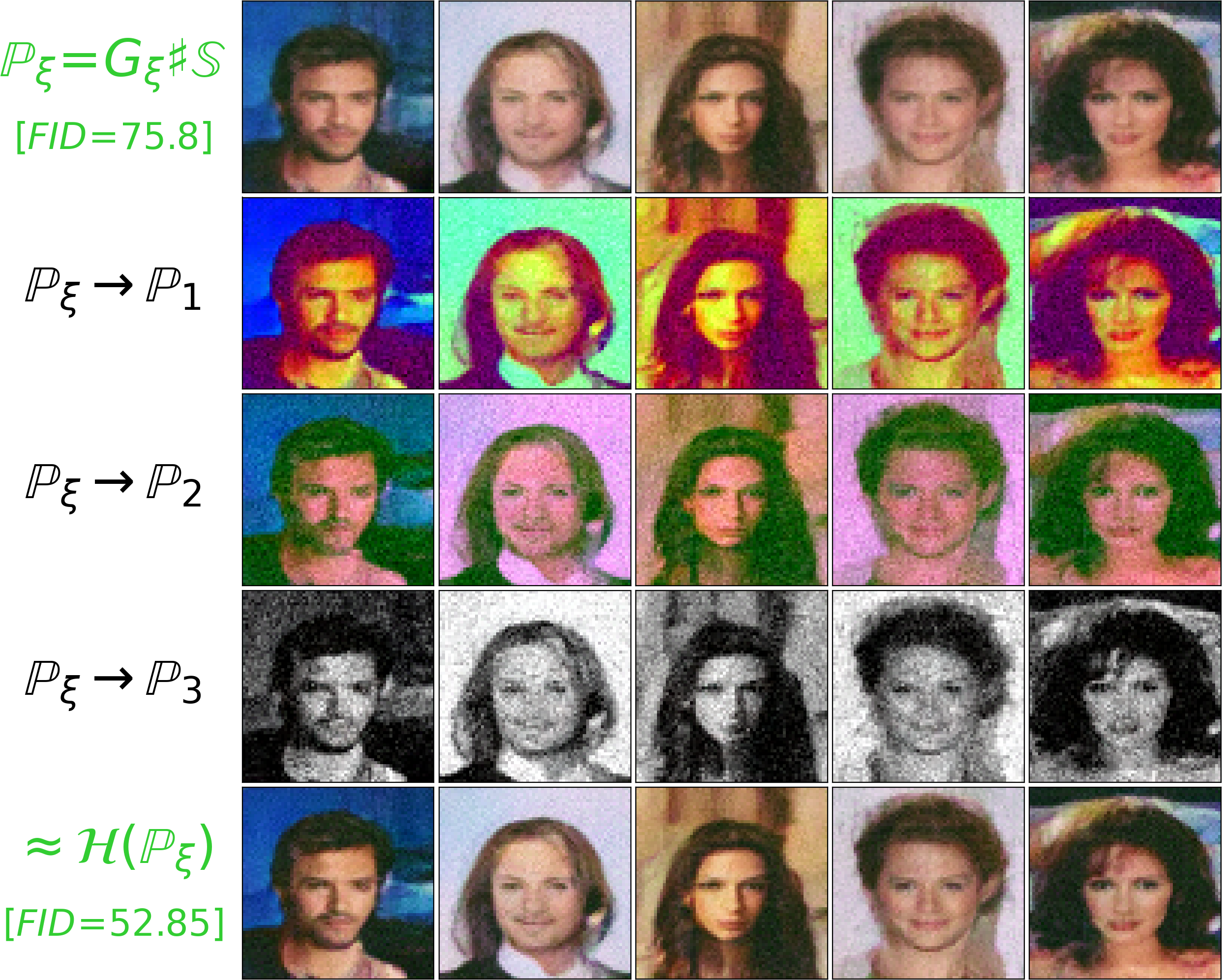
(a) Our Algorithm 1.

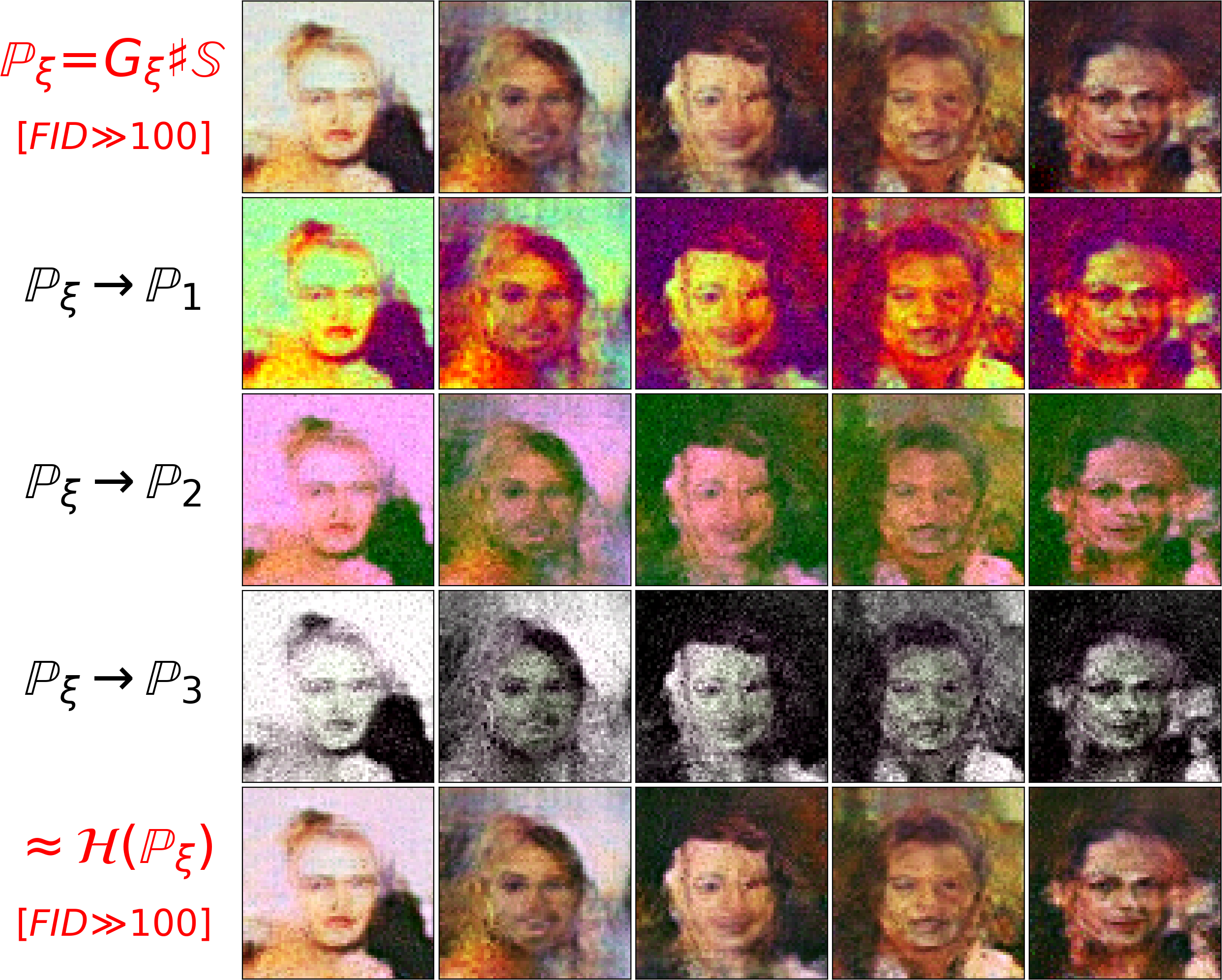
(b) Competitive $[\text{SC}\mathbb{W}_{2}\text{B}]$ algorithm.

Figure 5: The barycenter and maps to input measures estimated by barycenter algorithms. The 1st line shows generated samples $\mathbb{P}_{\xi}=G_{\xi}\sharp\mathbb{S}\approx\mathbb{P}_{\text{Celeba}}$. Lines 2-4 show maps $\widehat{T}_{\mathbb{P}_{\xi}\rightarrow\mathbb{P}_{n}}$. The last line shows the average map $\sum_{n=1}^{N}\alpha_{n}\widehat{T}_{\mathbb{P}_{\xi}\rightarrow\mathbb{P}_{n}}$.

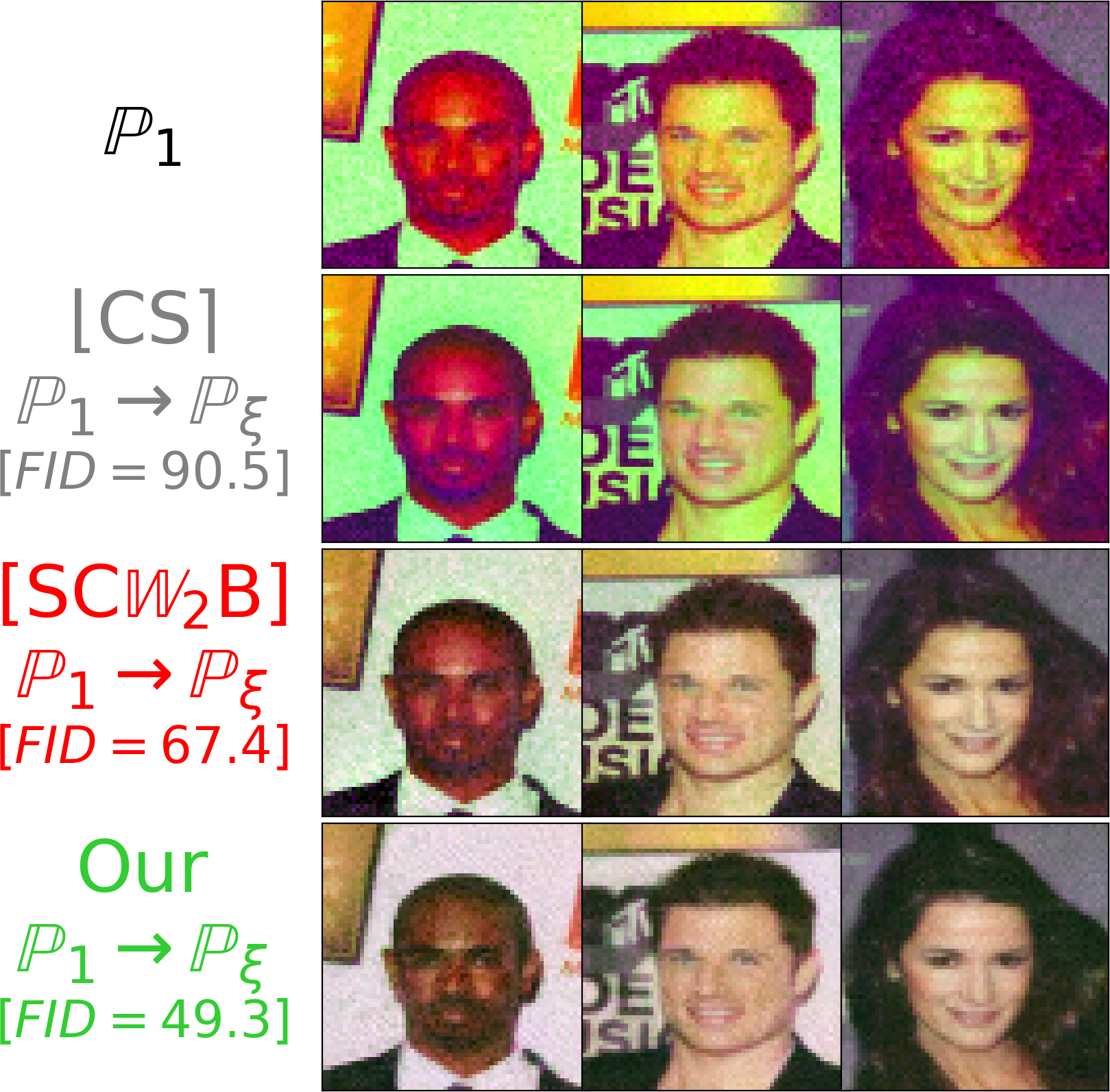
(a) Maps from $\mathbb{P}_{1}$ to the barycenter.

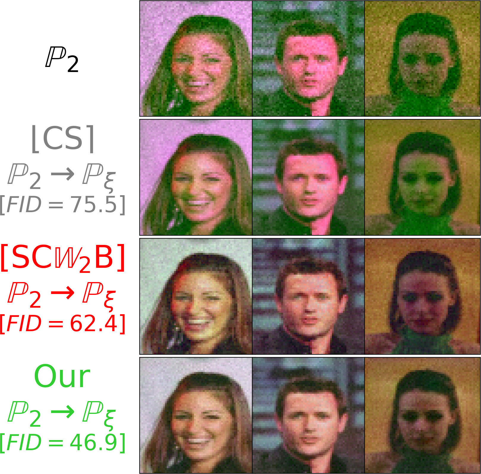
(b) Maps from $\mathbb{P}_{2}$ to the barycenter.

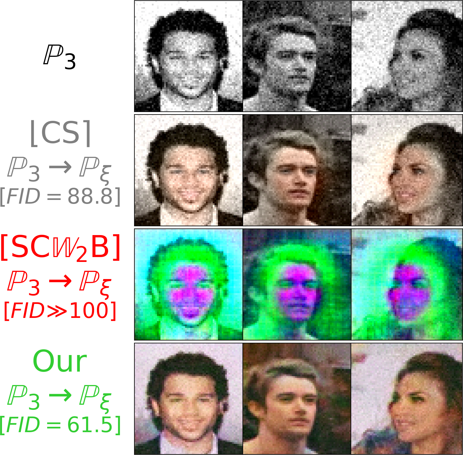
(c) Maps from $\mathbb{P}_{3}$ to the barycenter.

Figure 6: Maps from inputs $\mathbb{P}_{n}$ to the barycenter $\overline{\mathbb{P}}$ estimated by the barycenter algorithms in view. For comparison with the original barycenter images, the faces are the same as in Figure 4.

Method		FID$\downarrow$
$[\text{SC}\mathbb{W}_{2}B]$	$G_{\xi}(z)$	156.3
	$\sum_{n=1}^{N}\alpha_{n}\widehat{T}_{\mathbb{P}_{\xi}\rightarrow\mathbb{P}_{n}}\big{(}G_{\xi}(z)\big{)}$	152.1
Ours	$G_{\xi}(z)$	75.8
	$\sum_{n=1}^{N}\alpha_{n}\widehat{T}_{\mathbb{P}_{\xi}\rightarrow\mathbb{P}_{n}}\big{(}G_{\xi}(z)\big{)}$	52.85

Table 1: FID scores of images from the learned barycenter.

Method		FID$\downarrow$
		$n=1$	$n=2$	$n=3$
$\lfloor\text{CS}\rceil$	$y+(\overline{\mu}-\mu_{n})$	90.5	75.5	88.8
$[\text{SC}\mathbb{W}_{2}B]$	$\widehat{T}_{\mathbb{P}_{n}\rightarrow\mathbb{P}_{\xi}}(y)$	67.4	62.4	319.62
Ours	$\widehat{T}_{\mathbb{P}_{n}\rightarrow\mathbb{P}_{\xi}}(y)$	49.3	46.9	61.5

Table 2: FID scores of images mapped from inputs $\mathbb{P}_{n}$.

6.2 Additional Experimental Results

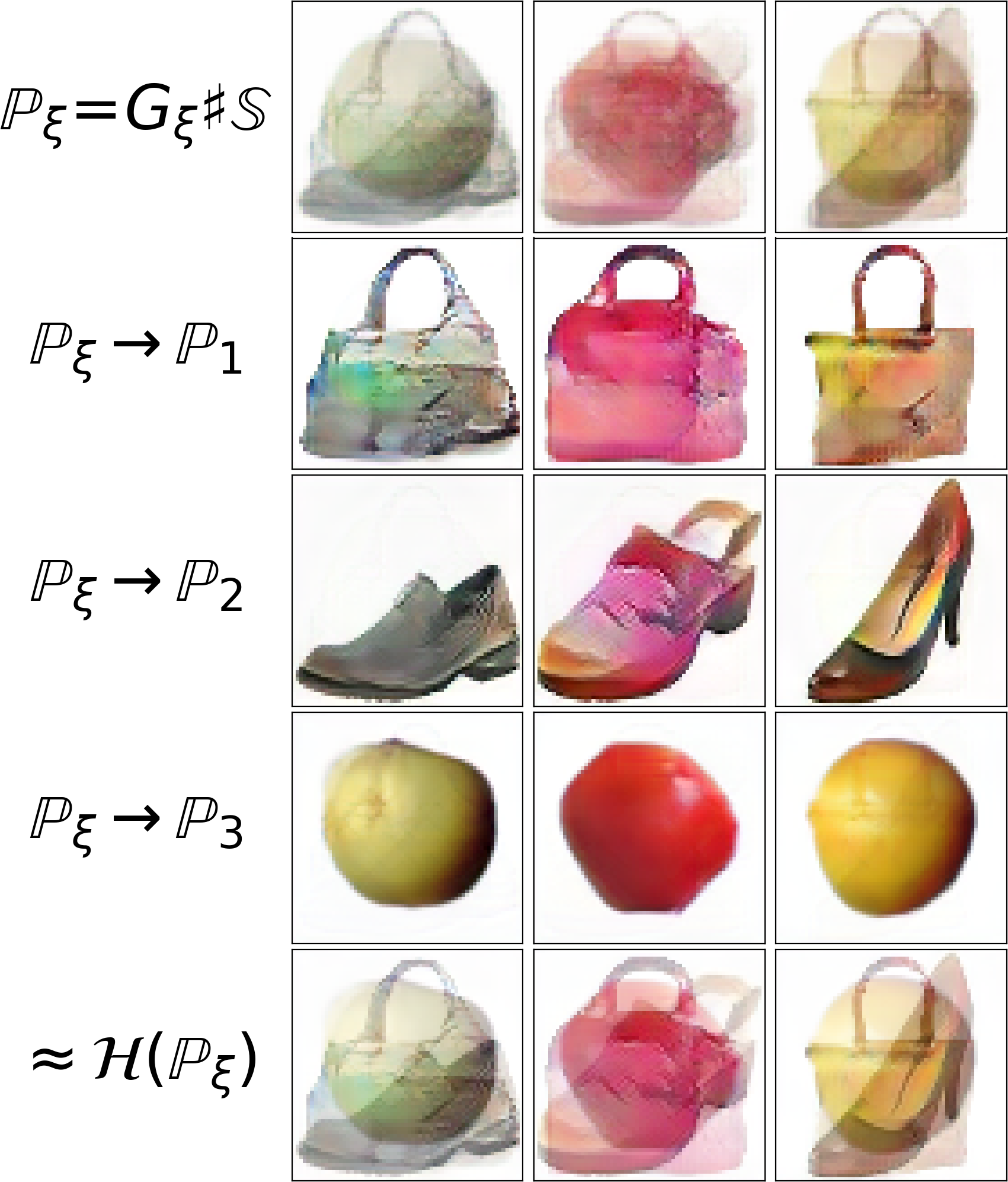
(a) Generated samples $\mathbb{P}_{\xi}\approx\overline{\mathbb{P}}$, fitted maps to each $\mathbb{P}_{n}$ and their average.

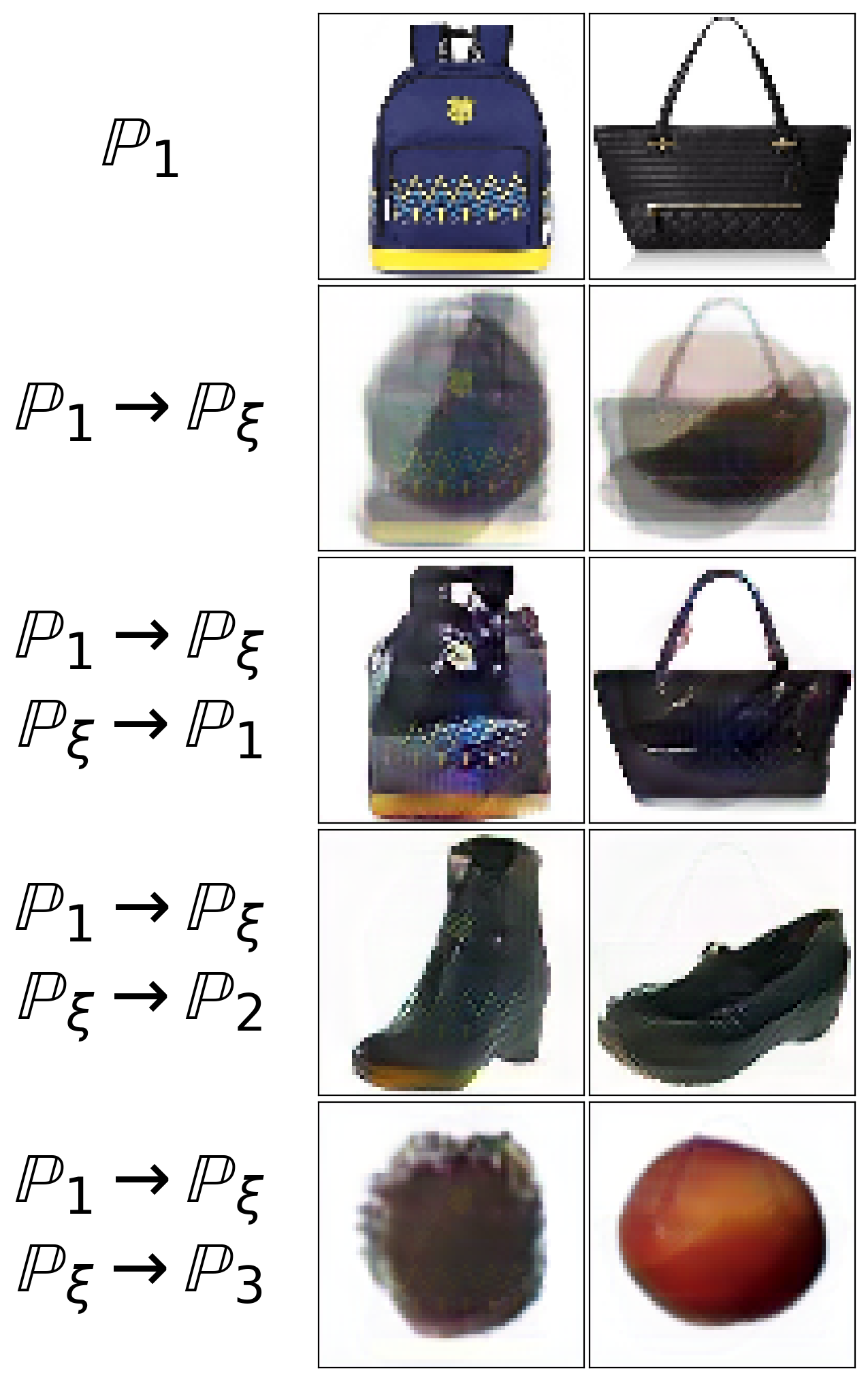
(b) Samples $y\sim\mathbb{P}_{1}$ mapped through $\mathbb{P}_{\xi}$ to each $\mathbb{P}_{n}$.

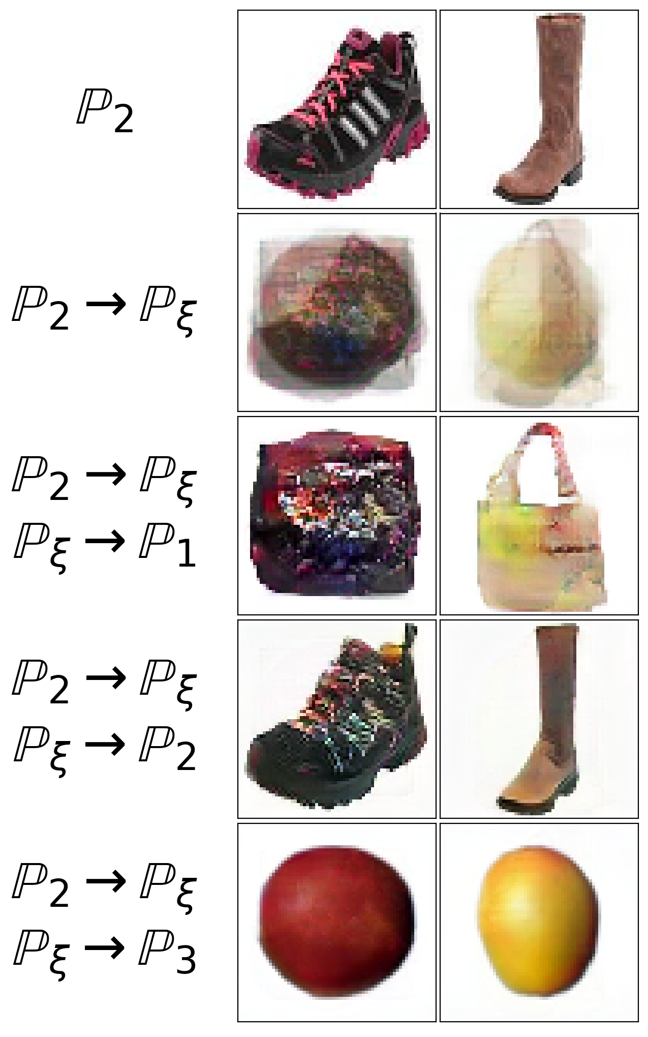
(c) Samples $y\sim\mathbb{P}_{2}$ mapped through $\mathbb{P}_{\xi}$ to each $\mathbb{P}_{n}$.

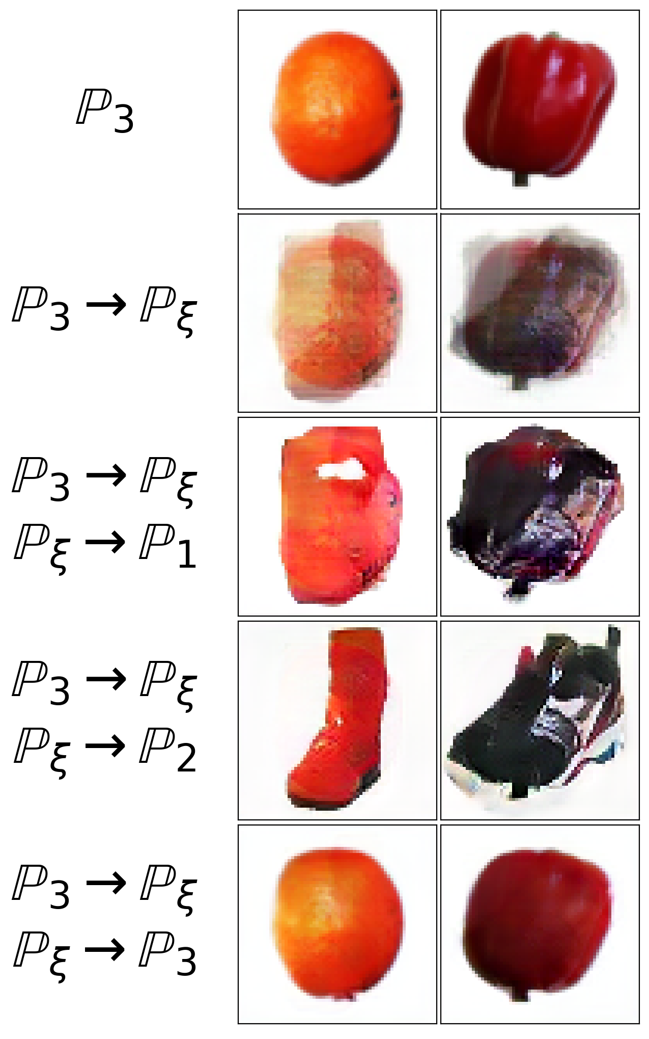
(d) Samples $y\sim\mathbb{P}_{3}$ mapped through $\mathbb{P}_{\xi}$ to each $\mathbb{P}_{n}$.

Figure 7: The barycenter of Handbags, Shoes, Fruit ($64\times 64$) datasets fitted by our Algorithm 1. We give the results of competitive [SC$\mathbb{W}_{2}$B] in Appendix B.4.

Different domains. To stress-test our algorithm 1, we compute the barycenters w.r.t. $(\alpha_{1},\alpha_{2},\alpha_{3})=(\frac{1}{3},\frac{1}{3},\frac{1}{3})$ of notably different datasets: 50K Shoes (yu2014fine, ), 138K Amazon Handbags and 90K Fruits (murecsan2017fruit, ). All the images are rescaled to $64\times 64$. The ground gruth barycenter is unknown, but one may imagine what it looks like. Due to (6), each barycenter image is a pixel-wise average of a shoe, a handbag and a fruit, which is supported by our result shown in Figure 7. In the same figure, we also show the maps between datasets through the barycenter (Figures 7(b), 7(c), 7(d)): this allows generation of images in other categories with styles similar to a given image. For instance, in Figure 7(d), we generate an orange bag and an orange shoe by pushing the image of an orange through the barycenter. We provide more examples in Figure 15 of Appendix C.5.

Extra results. In Appendix C.1, we compute the barycenters of toy 2D dsitributions. In Appendix C.2, we provide quantitative results for computing barycenters in the Gaussian case. In Appendix C.3, we test how our algorithm works as a generative model on the original CelebA dataset, i.e., when $N\!=\!1$ and $\mathbb{P}_{1}=\mathbb{P}_{\text{Celeba}}$. We show that in this case it achieves FID scores comparable to recent WGAN models. In Appendix C.4, similar to fan2020scalable , we compute barycenters of digit classes 0/1 of $32\times 32$ grayscale MNIST (lecun-mnisthandwrittendigit-2010, ). We also test our algorithm on FashionMNIST (xiao2017fashion, ) 10 classes dataset.

7 Discussion

Potential impact (algorithm). We present a scalable barycenter algorithm based on fixed-point iterations with many application prospects. For instance, in medical imaging, MRI is often acquired at multiple sites where the overlap of information (imaging, genetic, diagnosis) between any two sites is limited. Consequently, the data on each site may be biased and can cause generalizability and robustness issues when training models. The developed algorithm could help aggregate data from multiple sites and overcome the distributional shift issue across sites.

Potential impact (dataset). There is no high-dimensional dataset for the barycenter problem except for location-scattered cases (e.g. Gaussians), where the transport maps are always linear. Hence our proposed dataset fills an important gap, thereby allowing quantitative evaluation of future related methods. We expect our Ave, celeba! to become a standard dataset for evaluating continuous barycenter algorithms. In addition, we describe a generic recipe (5) to produce new datasets.

Limitations (algorithm). In our algorithm, the evolving measure $\mathbb{P}_{\xi}$ is not guaranteed to be continuous, while it is continuous in the underlying fixed point approach. To enforce the absolute continuity of $\mathbb{P}_{\xi}=G_{\xi}\sharp\mathbb{S}$, one may use an invertible network (etmann2020iunets, ) for $G_{\xi}$ and an absolutely continuous latent measure $\mathbb{S}$ in a latent space of dimension $H\!=\!D$. However, our results suggest this is unnecessary in practice — common GANs approaches also assume $H\!\ll\!D$. During the fixed-point iterations, the barycenter objective (5) decreases. However, there is no guarantee that the sequence of measures converges to a fixed point which is the barycenter. Identifying the precise conditions on the input measures and the initial point is an important future direction. Besides, our algorithm does not recover inverse OT maps $T_{\mathbb{P}_{n}\rightarrow\overline{\mathbb{P}}}$; we compute them with an OT solver as a follow-up. To avoid this step, one may consider using invertible neural nets (etmann2020iunets, ) to parametrize maps $T_{\theta_{n}}$ in our Algorithm 1.

Limitations (dataset). To create Ave, celeba! dataset (5), we compose ICNNs with decolorization, random reflections and permutations to simulate degraded images. It is unclear how to produce other practically interesting effects via ICNNs. It also remains an open question on how to better hide the information of the barycenter image in the constructed marginal measures. Studying these questions is an interesting future direction that can inspire benchmarking other OT problems.

Acknowledgements. E. Burnaev was supported by the Russian Foundation for Basic Research grant 21-51-12005 NNIO_a. A portion of this project was funded by the Skolkovo Institute of Science and Technology as part of the Skoltech NGP Program and funds were received by the Massachusetts Institute of Technology prior to September 1, 2022. Neither Mr. Li, nor any other MIT personnel, contributed to any substantive or artistic alteration or enhancement of this publication after August 31, 2022.

Checklist

1. For all authors…

   1. Do the main claims made in the abstract and introduction accurately reflect the paper’s contributions and scope?
      [Yes] See 1.

   2. Did you describe the limitations of your work?
      [Yes] See 7.

   3. Did you discuss any potential negative societal impacts of your work?
      [N/A]

   4. Have you read the ethics review guidelines and ensured that your paper conforms to them? [Yes]

2. If you are including theoretical results…

   1. Did you state the full set of assumptions of all theoretical results?
      [Yes] All the assumptions are stated in the main text.

   2. Did you include complete proofs of all theoretical results?
      [Yes] All the proofs are given in the appendices.

3. If you ran experiments…

   1. Did you include the code, data, and instructions needed to reproduce the main experimental results (either in the supplemental material or as a URL)?
      [Yes] The code and the instructions are included in the supplementary material. The datasets that we use are publicly available.

   2. Did you specify all the training details (e.g., data splits, hyperparameters, how they were chosen)?
      [Yes] See 6 and the supplementary material (appendices + code).

   3. Did you report error bars (e.g., with respect to the random seed after running experiments multiple times)?
      [No] Due to the well-known high computational complexity of learning generative models, most experiments (both with our method and alternatives) were conducted only once.

   4. Did you include the total amount of compute and the type of resources used (e.g., type of GPUs, internal cluster, or cloud provider)?
      [Yes] See the discussion in 6 and Appendices.

4. If you are using existing assets (e.g., code, data, models) or curating/releasing new assets…

   1. If your work uses existing assets, did you cite the creators?
      [Yes] See the discussion in section 6.

   2. Did you mention the license of the assets?
      [No] We refer to the datasets’ public pages.

   3. Did you include any new assets either in the supplemental material or as a URL?
      [Yes] See the supplementary material

   4. Did you discuss whether and how consent was obtained from people whose data you’re using/curating?
      [N/A]

   5. Did you discuss whether the data you are using/curating contains personally identifiable information or offensive content?
      [No] For CelebA faces dataset, we refer to the original authors publication.

5. If you used crowdsourcing or conducted research with human subjects…

   1. Did you include the full text of instructions given to participants and screenshots, if applicable?
      [N/A]

   2. Did you describe any potential participant risks, with links to Institutional Review Board (IRB) approvals, if applicable?
      [N/A]

   3. Did you include the estimated hourly wage paid to participants and the total amount spent on participant compensation?
      [N/A]

Appendix A Proofs

First, we recall basic properties of convex conjugate functions that we rely on in our proofs. Let ${\psi:\mathbb{R}^{D}\rightarrow\mathbb{R}}$ be a convex function and $\overline{\psi}$ be its convex conjugate. From the definition of $\overline{\psi}$, we obtain

$$\psi(x)+\overline{\psi}(y)\geq\langle x,y\rangle$$

for all $x,y\in\mathbb{R}^{D}.$ Assume that $\psi$ is differentiable and has an invertible gradient $\nabla\psi:\mathbb{R}^{D}\rightarrow\mathbb{R}^{D}$. The latter condition holds, e.g., for strongly convex functions. From the convexity of $\psi$, we derive

$${x=\operatorname*{arg\,max}_{x\in\mathbb{R}^{D}}[\langle x,y\rangle-\psi(x)]\Leftrightarrow y=\nabla\psi(x)\Leftrightarrow x=(\nabla\psi)^{-1}(y)},$$

which yields

$${\overline{\psi}(y)=\langle(\nabla\psi)^{-1}(x),x\rangle-\psi\big{(}(\nabla\psi)^{-1}(x))}.$$

In particular, the strict equality $\psi(x)+\overline{\psi}(y)=\langle x,y\rangle$ holds if and only if $y=\nabla\psi(x)$. By applying the same logic to $\overline{\psi}$, we obtain $(\nabla\overline{\psi})^{-1}=\nabla\psi$ and $(\nabla\psi)^{-1}=\nabla\overline{\psi}$, i.e., the gradients of conjugate functions are mutually inverse.

A.1 Proof of Lemma 1

Proof.

For each $n=1,2,\dots,N$ we perform the following evaluation:

$$\frac{\partial}{\partial\xi}\mathbb{W}_{2}^{2}(G_{\xi}\sharp\mathbb{S},\mathbb{P}_{n})=\int_{z}\mathbf{J}_{\xi}G_{\xi}(z)^{T}\nabla u_{n}^{*}\big{(}G_{\xi}(z)\big{)}d\mathbb{S}(z),$$ (13)

$$\int_{z}\mathbf{J}_{\xi}G_{\xi}(z)^{T}\big{(}G_{\xi}(z)-T_{\mathbb{P}_{\xi}\rightarrow\mathbb{P}_{n}}\big{(}G_{\xi}(z)\big{)}\bigg{)}d\mathbb{S}(z),$$ (14)

where $u_{n}^{*}$ is the optimal dual potential for $\mathbb{P}_{\xi}=G_{\xi}\sharp\mathbb{S}$ and $\mathbb{P}_{n}$. Equation (13) follows from [22, Equation 3]. Equation (14) follows from the property $\nabla u_{n}^{*}(x)=x-T_{\mathbb{P}_{\xi}\rightarrow\mathbb{P}_{n}}(x)$ connecting dual potentials and OT maps. We sum (14) for $n=1,\dots,N$ w.r.t. weights $\alpha_{n}$ with $\xi=\xi_{0}$ and obtain

$$\frac{\partial}{\partial\xi}\sum_{n=1}^{N}\alpha_{n}\mathbb{W}_{2}^{2}(G_{\xi}\sharp\mathbb{S},\mathbb{P}_{n})=\int_{z}\mathbf{J}_{\xi}G_{\xi_{0}}(z)^{T}\bigg{(}G_{\xi_{0}}(z)-\sum_{n=1}^{N}\alpha_{n}T_{\mathbb{P}_{\xi_{0}}\rightarrow\mathbb{P}_{n}}\big{(}G_{\xi_{0}}(z)\big{)}\bigg{)}d\mathbb{S}(z).$$ (15)

Note that (15) exactly matches the derivative of the left-hand side of (9) evaluated at $\xi=\xi_{0}$. ∎

A.2 Proof of Lemma 2

Proof.

First, we prove the congruence, i.e., $\beta\psi^{l}(x)+(1-\beta)\psi^{r}(x)=\frac{\|x\|^{2}}{2}$ for all $x\in\mathbb{R}^{D}$.

$$\beta\psi^{l}(x)+(1-\beta)\psi^{r}(x)=$$

$$\beta\max_{y_{1}\in\mathbb{R}^{D}}\big{[}\langle x,y_{1}\rangle-\overline{\psi^{l}}(y_{1})\big{]}+(1-\beta)\max_{y_{2}\in\mathbb{R}^{D}}\big{[}\langle x,y_{2}\rangle-\overline{\psi^{r}}(y_{2})\big{]}=$$ (16)

$$\beta\max_{y_{1}\in\mathbb{R}^{D}}\big{[}\langle x,y_{1}\rangle-\beta\frac{\|y_{1}\|^{2}}{2}-(1-\beta)\psi(y_{1})\big{]}+$$

$$(1-\beta)\max_{y_{2}\in\mathbb{R}^{D}}\big{[}\langle x,y_{2}\rangle-(1-\beta)\frac{\|y_{2}\|^{2}}{2}-\beta\overline{\psi}(x)\big{]}=$$

$$\max_{y_{1},y_{2}\in\mathbb{R}^{D}}\big{[}\langle x,\beta y_{1}+(1-\beta)y_{2}\rangle-\beta^{2}\frac{\|y_{1}\|^{2}}{2}-(1-\beta)^{2}\frac{\|y_{2}\|^{2}}{2}-\beta(1-\beta)(\psi(y_{1})+\overline{\psi}(y_{2}))\big{]}\leq$$ (17)

$$\max_{y_{1},y_{2}\in\mathbb{R}^{D}}\big{[}\langle x,\beta y_{1}+(1-\beta)y_{2}\rangle-\beta^{2}\frac{\|y_{1}\|^{2}}{2}-(1-\beta)^{2}\frac{\|y_{2}\|^{2}}{2}-\beta(1-\beta)\langle y_{1},y_{2}\rangle\big{]}=$$

$$\max_{y_{1},y_{2}\in\mathbb{R}^{D}}\frac{\|x\|^{2}}{2}-\frac{1}{2}\|x-(\beta y_{1}+(1-\beta)y_{2})\|^{2}\leq\frac{\|x\|^{2}}{2}.$$ (18)

First, we substitute $(y_{1},y_{2})=(y^{l},\nabla\psi(y^{l}))$. For this pair, $x=\nabla\overline{\psi^{l}}(y^{l})=\beta y^{l}+(1-\beta)\nabla\psi(y^{l})$, which results in $x=\beta y_{1}+(1-\beta)y_{2}$. Moreover, since $y_{2}=\nabla\psi(y_{1})$, we have $\psi(y_{1})+\overline{\psi}(y_{2})=\langle y_{1},y_{2}\rangle$. As the consequence, both inequalities (17) and (18) turn to strict equalities yielding congruence of $\psi^{l},\psi^{r}$. From (10), the smoothness and strong convexity of $\psi$ imply that $\psi^{l}$ and $\psi^{r}$ are smooth. Consequently, $\overline{\psi^{l}}$ and $\overline{\psi^{l}}$ are strongly convex. Thus, the maximizer of (16) is unique. We know the maximum of (16) is attained at $(y_{1},y_{2})=(\nabla\psi^{l}(x),\nabla\psi^{r}(x))=(y^{l},y^{r})$. We conclude $(y^{l},y^{r})=(y^{l},\nabla\psi(y^{l}))$, i.e., $y^{r}=\nabla\psi(y^{l})$. Finally, $y^{l}=\nabla\psi^{l}(x)\Leftrightarrow x=\nabla\overline{\psi^{l}}(y^{l})\Leftrightarrow y^{l}=\max\limits_{y\in\mathbb{R}^{D}}\big{[}\langle x,y\rangle-\overline{\psi^{l}}(y)\big{]}$, which matches (11). ∎

A.3 Proof of Lemma 3

Proof.

First, we check that $\sum_{n=1}^{N}\alpha_{n}$ indeed equals 1:

$$\sum_{n=1}^{N}\alpha_{n}=\sum_{n=1}^{N}\sum_{m=1}^{M}w_{m}\big{[}\beta_{m}\gamma^{l}_{nm}+(1-\beta_{m})\gamma^{r}_{nm}\big{]}=$$

$$\sum_{m=1}^{M}\big{[}w_{m}\beta_{m}\underbrace{\sum_{n=1}^{N}\gamma^{l}_{nm}}_{=1}\big{]}+\sum_{m=1}^{M}\big{[}w_{m}(1-\beta_{m})\underbrace{\sum_{n=1}^{N}\gamma^{r}_{nm}}_{=1}\big{]}=$$

$$\sum_{m=1}^{M}w_{m}\beta_{m}+\sum_{m=1}^{M}w_{m}(1-\beta_{m})=\sum_{m=1}^{M}w_{m}\big{(}\beta_{m}+(1-\beta_{m})\big{)}=\sum_{m=1}^{M}w_{m}=1.$$ (19)

Next, we check that $\psi_{1},\dots,\psi_{N}$ are congruent w.r.t. weights $\alpha_{1},\dots,\alpha_{N}$:

$$\sum_{n=1}^{N}\alpha_{n}\psi_{n}(x)=\sum_{n=1}^{N}\sum_{m=1}^{M}w_{m}\big{[}\beta_{m}\gamma^{l}_{nm}\cdot\psi_{m}^{l}(x)+(1-\beta_{m})\gamma^{r}_{nm}\cdot\psi_{m}^{r}(x)\big{]}=$$

$$\sum_{m=1}^{M}\big{[}w_{m}\beta_{m}\psi_{m}^{l}(x)\underbrace{\sum_{n=1}^{N}\gamma^{l}_{nm}}_{=1}\big{]}+\sum_{m=1}^{M}\big{[}w_{m}(1-\beta_{m})\psi_{m}^{r}(x)\underbrace{\sum_{n=1}^{N}\gamma^{r}_{nm}}_{=1}\big{]}=$$

$$\sum_{m=1}^{M}\big{[}w_{m}\underbrace{\big{(}\beta_{m}\psi_{m}^{l}(x)+(1-\beta_{m})\psi^{r}(x)\big{]}}_{=\frac{\|x\|^{2}}{2}}=\sum_{m=1}^{M}w_{m}\frac{\|x\|^{2}}{2}=\frac{\|x\|^{2}}{2}.$$

∎

Appendix B Experimental Details

B.1 Ave, celeba! Dataset Creation

The initialization of random permutations $\sigma_{m}$ and reflections $s_{m}$ (for $m=1,2$) as well as the random split of CelebA dataset into 3 parts (each containing $\approx 67K$ images) are hardcoded in our provided script for producing Ave, celeba! dataset. To initialize ICNN_m (for $m=1,2$), we use use ConvICNN64 [29, Appendix B.1] checkpoints Early_v1_conj.pt, Early_v2_conj.pt from the official Wasserstein-2 benchmark repository.

We rescale Celeba images to $64\times 64$ by using imresize from scipy.misc. To create empirical samples from input distributions $\mathbb{P}_{n}$ by using the rescaled CelebA dataset, we compute the gradient maps $\nabla\psi_{n}(x)$ ($n=1,2,3$) in Lemma 3 for images $x$ in the CelebA dataset. This computation implies computing gradient maps $\nabla\psi_{m}^{l}(x)$ and $\nabla\psi_{m}^{r}(x)$ for each base function $\psi_{m}^{0}$ ($m=1,2$) and summing them with respective coefficients (12). Following our Lemma 2, we compute $y^{l}_{m}\stackrel{{\scriptstyle\text{def}}}{{=}}\nabla\psi_{m}^{l}(x)$ by solving a concave optimization problem (11) over the space of images. We solve this problem with the gradient descent. We use Adam optimizer [26] with default betas, $lr=2\cdot 10^{-2}$ and do $1000$ gradient steps. To speed up the computation, we simultaneously solve the problem for a batch of $256$ images $x$ from CelebA dataset. Then we compute $y^{r}\stackrel{{\scriptstyle\text{def}}}{{=}}\nabla\psi_{m}^{r}(x)$ as $y^{r}=\nabla\psi_{m}(y^{l})$ (Lemma 2).

Computational complexity. Producing Ave, celeba! takes about $1,5$ days on a GPU GTX 1080 ti.

B.2 Hyperparameters (Algorithm 1, Main Training)

We provide the hyperparameters of all the experiments with algorithm 1 in Table 3. The column total iters shows the sum of gradient steps over generator $G_{\xi}$ and each of $N$ potentials $v_{\omega_{n}}$ in OT solvers.

Optimization. We use Adam optimizer with the default betas. During training, we decrease the learning rates of the generator $G_{\xi}$ and each potential $v_{\omega_{n}}$ every 10K steps of their optimizers. In the Gaussian case, we use a single GPU GTX 1080ti. In all other cases we split the batch over 4$\times$GPU GTX 1080ti (nn.DataParallel in PyTorch).

Neural Network Architectures. In the Gaussian case, we use In the evaluation in the Gaussian case, we use sequential fully-connected neural networks with ReLU activations for the generator $G_{\xi}:\mathbb{R}^{D}\rightarrow\mathbb{R}^{D}$, potentials $v_{\omega_{n}}:\mathbb{R}^{D}\rightarrow\mathbb{R}$ and transport maps ${T_{\theta_{n}}:\mathbb{R}^{D}\rightarrow\mathbb{R}^{D}}$. For all the networks the sizes of hidden layers are:

$$[\max(100,2D),\max(100,2D),\max(100,2D)].$$

Working with images, we use the ResNet generator and discriminator architectures of WGAN-QC [35] for our generator $G_{\xi}$ and potentials $v_{\omega_{n}}$ respectively. As the maps $T_{\theta_{n}}$, we use U-Net [52].

Generator regression loss. In the Gaussian case and experiments with grayscale images (MNIST, FashionMNIST), we use mean squared loss for generator regression. In other experiments, we use the perceptual mean squared loss based on the features of the pre-trained VGG-16 network [57]. The loss is hardcoded in the implementation.

Data pre-processing. In all experiments with images we normalize them to $[-1,1]$. We rescale MNIST and FashionMNIST images to $32\times 32$. In all other cases, we rescale images to $64\times 64$. Note that Fruit360 dataset originally contains $114\times 114$ images; before rescaling, we add white color padding to make the images have the size $128\times 128$. Working with Ave, celeba! dataset, we additionally shift each subset $\mathbb{P}_{n}$ by $(\overline{\mu}-\mu_{n})$, i.e., we train the models on the $\lceil\text{CS}\rfloor$ baseline. This helps the models to avoid learning the shift.

Computational complexity. The most challenging experiments (Ave, celeba! and Handbags, Shoes, Fruit) take about 2-3 days to converge on $4\times$GPU GTX 1080 ti. Other experiments converge faster.

Experiment

D

H

$N$

$G_{\xi}$

$v_{\omega_{n}}$

$T_{\theta_{n}}$

$k_{G}$

$k_{v}$

$k_{T}$

$lr_{G}$

$lr_{v}$

$lr_{T}$

$\ell$

Total iters

Batch size

Toy 2D

2

2

3

MLP

MLP

50

50

10

$1\cdot 10^{-4}$

$1\cdot 10^{-3}$

$1\cdot 10^{-3}$

MSE

12K

1024

Gaussians

2-128

2-128

4

MLP

MLP

10

$1\cdot 10^{-4}$

$1\cdot 10^{-3}$

$1\cdot 10^{-3}$

12K

1024

MNIST 0/1

1024

16

2

ResNet

UNet

15

$1\cdot 10^{-4}$

$1\cdot 10^{-4}$

$1\cdot 10^{-4}$

60K

64

FashionMNIST

10

10

$1\cdot 10^{-4}$

$1\cdot 10^{-4}$

$1\cdot 10^{-4}$

100K

Bags, Shoes, Fruit

12288

128

3

10

$3\cdot 10^{-4}$

$3\cdot 10^{-4}$

$3\cdot 10^{-4}$

VGG

36K

Ave, celeba!

3

10

$3\cdot 10^{-4}$

$3\cdot 10^{-4}$

$3\cdot 10^{-4}$

60K

Celeba

1

15

$1\cdot 10^{-4}$

$1\cdot 10^{-4}$

$1\cdot 10^{-4}$

80K

Celeba (fixed $G$)

1

0

15

$1\cdot 10^{-4}$

$1\cdot 10^{-4}$

$1\cdot 10^{-4}$

120K

Table 3: Hyperparameters that we use in the experiments with our algorithm 1.

B.3 Hyperparameters (Algorithm 2, Learning Maps to the Barycenter)

After using the main algorithm 1 to train $G_{\xi}$, we use algorithm 2 to extract the inverse optimal maps $\mathbb{P}_{n}\rightarrow\mathbb{P}_{\xi}$. We detail the hyperparameters in Table 4 below. In all the cases we use Adam optimizer with the default betas. The column total iters show the number of update steps for each $v^{\text{inv}}_{\omega_{n}^{\prime}}$.

Experiment	D	$N$	$v_{\omega_{n}}$	$T_{\theta_{n}}$	$k_{T}$	$lr_{v}$	$lr_{T}$	Total iters	Batch size
Toy 2D	2	2	MLP	MLP	10	$1\cdot 10^{-3}$	$1\cdot 10^{-3}$	10k	1024
MNIST 0/1	1024	2	ResNet	UNet	10	$1\cdot 10^{-4}$	$1\cdot 10^{-4}$	4k	64
FashionMNIST		10						4k
Bags, Shoes, Fruit	12288	3						20K
Ave, celeba!		3						12K

Table 4: Hyperparameters that we use in the experiments with algorithm 2

Input : latent $\mathbb{S}$ and input $\mathbb{P}_{1},\dots,\mathbb{P}_{N}$ measures; pretrained generator $G_{\xi}:\mathbb{R}^{H}\rightarrow\mathbb{R}^{D}$ satisfying $G_{\xi}\sharp\mathbb{S}\approx\overline{\mathbb{P}}$;

mapping networks $T^{\text{inv}}_{\theta_{1}^{\prime}},\dots,T^{\text{inv}}_{\theta_{N}^{\prime}}:\mathbb{R}^{D}\rightarrow\mathbb{R}^{D}$; potentials $v^{\text{inv}}_{\omega_{1}^{\prime}},\dots,v_{\omega_{N}^{\prime}}^{\text{inv}}:\mathbb{R}^{D}\rightarrow\mathbb{R}$;

number of inner iterations for training transport maps: $K_{T}$;

Output : OT maps satisfying $T_{\theta_{n}^{\prime}}^{\text{inv}}\sharp\mathbb{P}_{n}\approx\mathbb{P}_{\xi}=(G_{\xi}\sharp\mathbb{S})\approx\overline{\mathbb{P}}$;

repeat

     for $n=1,2,\dots,N$ do

         Sample batches $Z\!\sim\!\mathbb{S}$, $Y\!\sim\!\mathbb{P}_{n}$; $X\!\leftarrow\!G_{\xi}(Z)$;

         $\mathcal{L}_{v}\leftarrow\frac{1}{|Y|}\sum\limits_{y\in Y}v^{\text{inv}}_{\omega_{n}^{\prime}}\big{(}T^{\text{inv}}_{\theta_{n}^{\prime}}(y)\big{)}-\frac{1}{|X|}\sum\limits_{x\in X}v^{\text{inv}}_{\omega_{n}^{\prime}}\big{(}x\big{)}$;

         Update $\omega_{n}^{\prime}$ by using $\frac{\partial\mathcal{L}_{v}}{\partial\omega_{n}^{\prime}}$;

        

        for $k_{T}=1,2,\dots,K_{T}$ do

             Sample batch $Y\!\sim\!\mathbb{P}_{n}$;

             ${\mathcal{L}_{T}\!=\!\frac{1}{|Y|}\!\sum\limits_{y\in Y}\!\big{[}\frac{1}{2}\|y\!-\!T^{\text{inv}}_{\theta_{n}^{\prime}}(y)\|^{2}\!-\!v^{\text{inv}}_{\omega_{n}^{\prime}}\!\big{(}T^{\text{inv}}_{\theta_{n}^{\prime}}(y)\big{)}\!\big{]}}$;

             Update $\theta_{n}^{\prime}$ by using $\frac{\partial\mathcal{L}_{T}}{\partial\theta_{n}^{\prime}}$;

            

        

    

until not converged;

Algorithm 2 Learning maps from input measures to the learned barycenter $\mathbb{P}_{\xi}\approx\overline{\mathbb{P}}$ with $\lceil\text{MM:R}\rceil$ OT solver.

B.4 Hyperparameters of competitive [SC$\mathbb{W}_{2}$B] algorithm

On Ave, celeba! we use [19, Algorithm 1] with $k_{3}=50000$, $k_{2}=k_{1}=10$. The optimizer, the learning rates and the generator network are the same as in our algorithm. However, for the potentials (OT solver), we use ICNN architecture as it is required by their method. We use ConvICNN64 [29, Appendix B.1] architecture. For handbags, shoes, fruit (Figure 8), the parameters are the same.

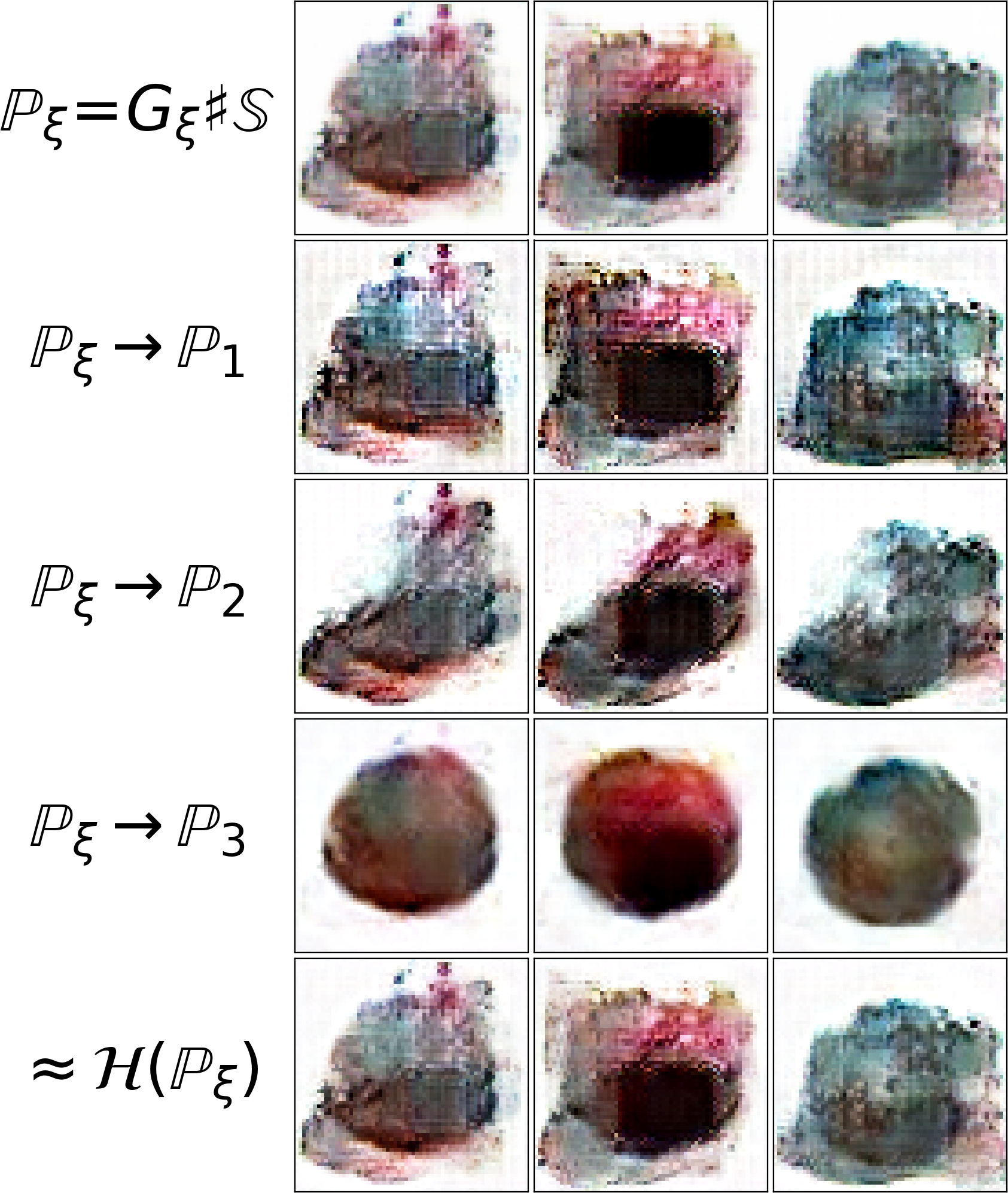
(a) Generated samples $\mathbb{P}_{\xi}\approx\overline{\mathbb{P}}$, fitted maps to each $\mathbb{P}_{n}$ and their average.

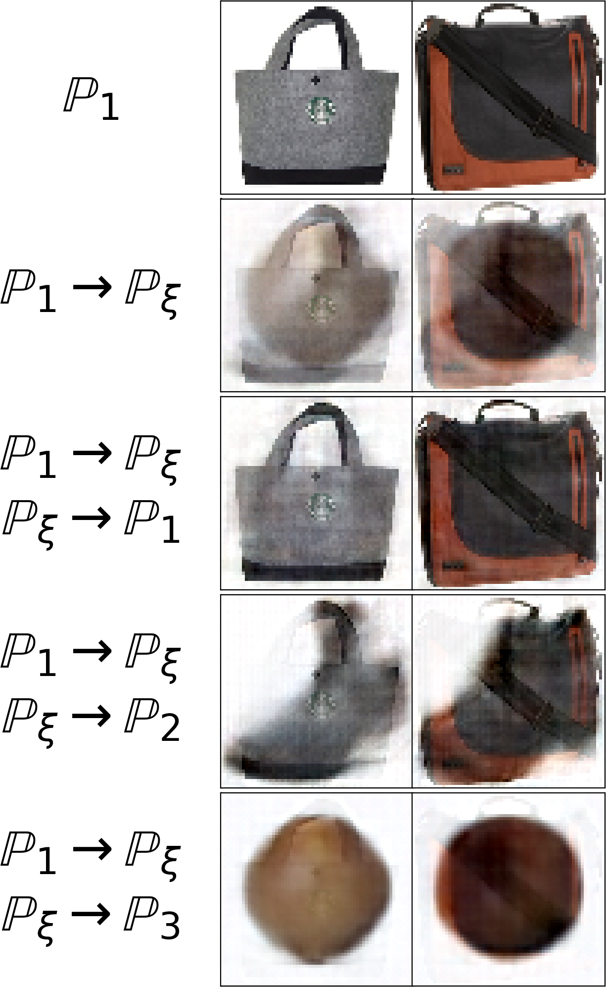
(b) Samples $y\sim\mathbb{P}_{1}$ mapped through $\mathbb{P}_{\xi}$ to each $\mathbb{P}_{n}$.

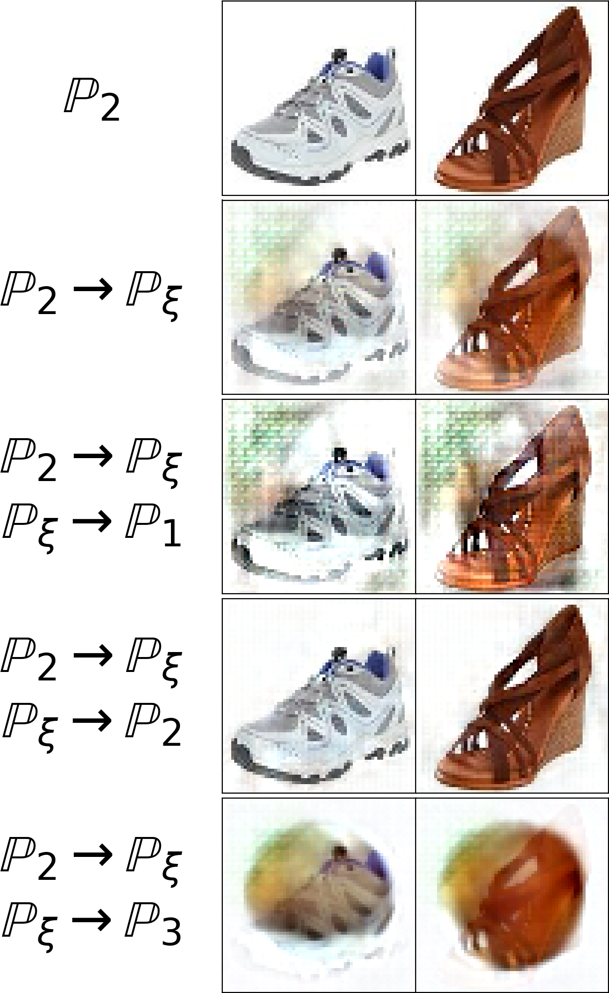
(c) Samples $y\sim\mathbb{P}_{2}$ mapped through $\mathbb{P}_{\xi}$ to each $\mathbb{P}_{n}$.

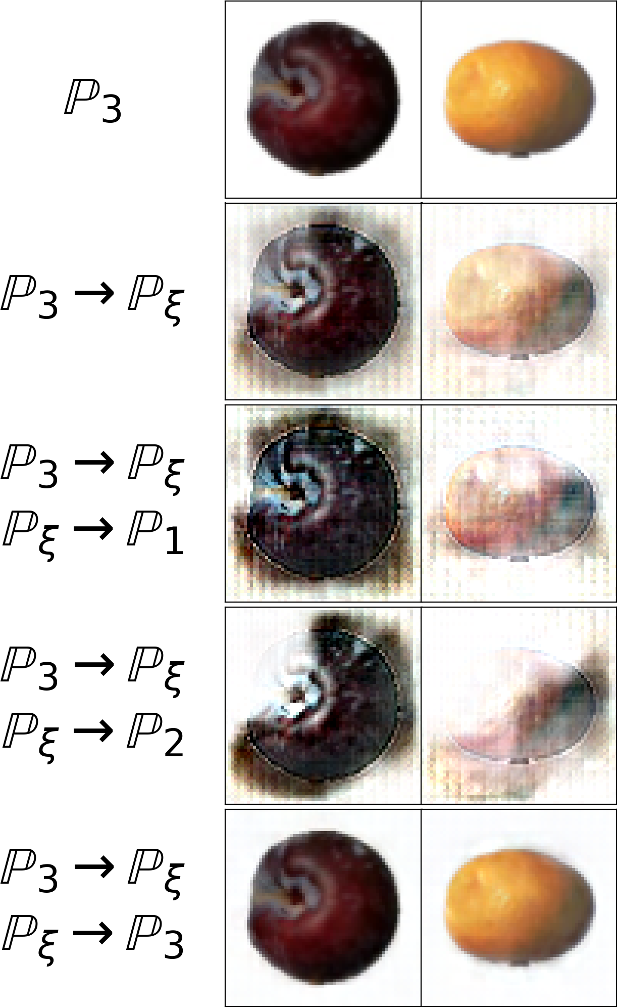
(d) Samples $y\sim\mathbb{P}_{3}$ mapped through $\mathbb{P}_{\xi}$ to each $\mathbb{P}_{n}$.

Figure 8: The barycenter of Handbags, Shoes, Fruit ($64\times 64$) datasets fitted by competitive [SC$\mathbb{W}_{2}$B].

Appendix C Additional Experimental Results

C.1 Toy Experiments

In this section, we provide examples of barycenters computed by our Algorithm for 2D location-scatter cases. To produce the location-scatter population of distributions and compute their ground truth barycenters, we employ the publicly available code of $[\text{C}\mathbb{W}_{2}\text{B}]$ paper [30]. The hyper-parameters of our Algorithm 1 (learning the barycenter and maps to input measures) and Algorithm 2 ($\lceil\text{MM:R}\rfloor$ solver, learning the inverse maps) are given in Tables 3 and 4, respectively. For evaluation, we consider two location-scatter populations produced by a rectangle and a swiss-roll respectively [30, 5]. The computed barycenters and maps to/from the input distributions are shown in Figures 9, 10.

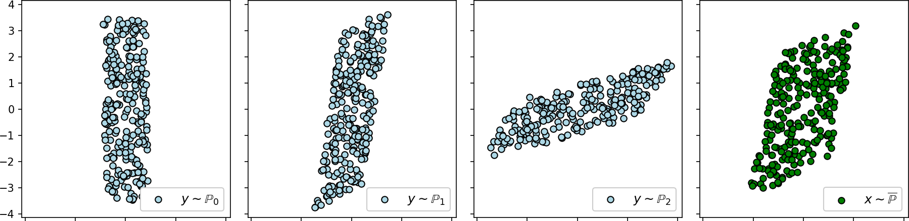
(a) Input measures $\mathbb{P}_{\xi}$ and their ground truth barycenter $\overline{\mathbb{P}}$ w.r.t. weights $\alpha_{1}=\alpha_{2}=\alpha_{3}=\frac{1}{3}$.

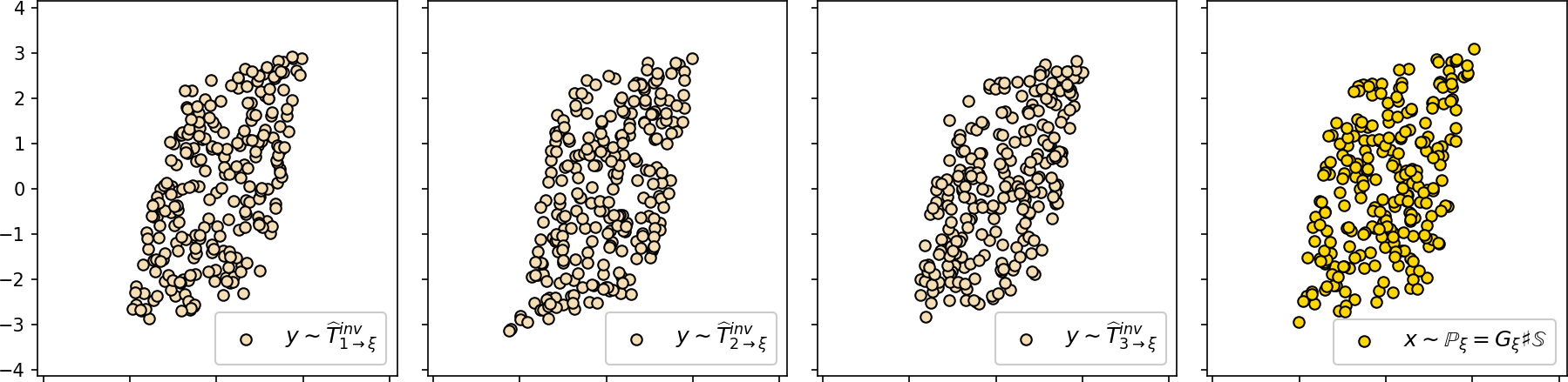
(b) Learned maps $\mathbb{P}_{n}\rightarrow\mathbb{P}_{\xi}$ from the input measures and the generated barycenter $\mathbb{P}_{\xi}=G_{\xi}\sharp\mathbb{S}$.

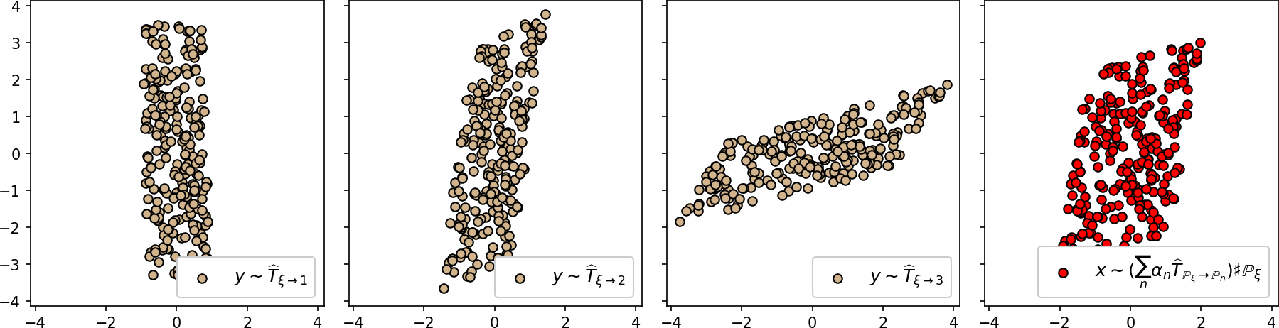
(c) Learned maps $\mathbb{P}_{\xi}\rightarrow\mathbb{P}_{n}$ from the generated barycenter $\mathbb{P}_{\xi}=G_{\xi}\sharp\mathbb{S}$ to the input measures $\mathbb{P}_{n}$and their weighted average map $\sum_{n=1}^{N}\big{[}\alpha_{n}\widehat{T}_{\mathbb{P}_{\xi}\rightarrow\mathbb{P}_{n}}\big{]}\sharp\mathbb{P}_{\xi}$.

Figure 9: The results of applying our algorithm to compute the barycenter of a 2Dlocation-scatter population produced by a rectangle.

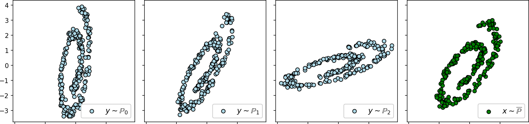
(a) Input measures $\mathbb{P}_{\xi}$ and their ground truth barycenter $\overline{\mathbb{P}}$ w.r.t. weights $\alpha_{1}=\alpha_{2}=\alpha_{3}=\frac{1}{3}$.

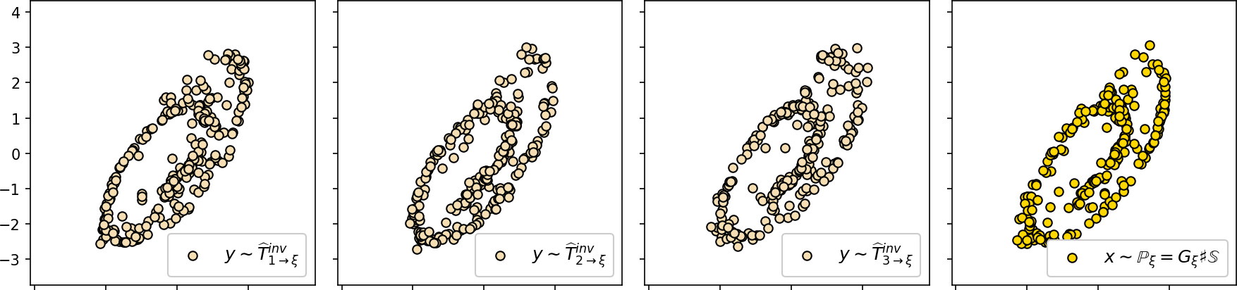
(b) Learned maps $\mathbb{P}_{n}\rightarrow\mathbb{P}_{\xi}$ from the input measures and the generated barycenter $\mathbb{P}_{\xi}=G_{\xi}\sharp\mathbb{S}$.

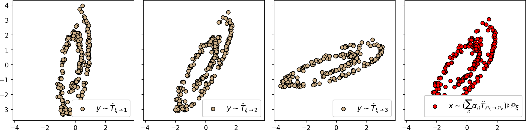
(c) Learned maps $\mathbb{P}_{\xi}\rightarrow\mathbb{P}_{n}$ from the generated barycenter $\mathbb{P}_{\xi}=G_{\xi}\sharp\mathbb{S}$ to the input measures $\mathbb{P}_{n}$and their weighted average map $\sum_{n=1}^{N}\big{[}\alpha_{n}\widehat{T}_{\mathbb{P}_{\xi}\rightarrow\mathbb{P}_{n}}\big{]}\sharp\mathbb{P}_{\xi}$.

Figure 10: The results of applying our algorithm to compute the barycenter of a 2Dlocation-scatter population produced by a Swiss roll.

C.2 Location-Scatter Case

Similar to [30, 19], we consider location-scatter cases for which the true barycenter can be computed [3, §4]. Let $\mathbb{P}_{0}\in\mathcal{P}_{2,\text{ac}}(\mathbb{R}^{D})$ and define the following location-scatter family of distributions $\mathcal{F}(\mathbb{P}_{0})=\{f_{S,u}\sharp\mathbb{P}_{0}\mbox{ }|\mbox{ }S\in\mathcal{M}^{+}_{D\times D},u\in\mathbb{R}^{D}\},$ where $f_{S,u}:\mathbb{R}^{D}\rightarrow\mathbb{R}^{D}$ is a linear map $f_{S,u}(x)=Sx+u$ with positive definite matrix $S\in\mathcal{M}^{+}_{D\times D}$. When $\{\mathbb{P}_{n}\}\subset\mathcal{F}(\mathbb{P}_{0})$, their barycenter $\overline{\mathbb{P}}$ is also an element of $\mathcal{F}(\mathbb{P}_{0})$ and can be computed via fixed-point iterations [3]. We use ${N=4}$ measures with weights ${(\alpha_{1},\dots,\alpha_{4})=(\frac{1}{10},\frac{2}{10},\frac{3}{10},\frac{4}{10})}$. We consider two choices for $\mathbb{P}_{0}$: the $D$-dimensional standard Gaussian and the uniform distribution on $[-\sqrt{3},+\sqrt{3}]^{D}$. By using the publicly available code of [30], we construct $\mathbb{P}_{n}$ as $f_{S_{n}^{T}\Lambda S_{n},0}\sharp\mathbb{P}_{0}\in\mathcal{F}(\mathbb{P}_{0})$, where $S_{n}$ is a random rotation matrix and $\Lambda$ is diagonal with entries $[\frac{1}{2}b^{0},\frac{1}{2}b^{1},\dots,2]$ where $b=\sqrt[D-1]{4}$. We quantify the generated barycenter $G_{\xi}\sharp\mathbb{S}$ with the Bures-Wasserstein Unexplained Variance Percentage [30, 5]:

$$\text{B}\mathbb{W}_{2}^{2}\text{-UVP}(G_{\xi}\sharp\mathbb{S},\overline{\mathbb{P}})=100\cdot\text{B}\mathbb{W}_{2}^{2}(G_{\xi}\sharp\mathbb{S},\overline{\mathbb{P}})/\big{[}\frac{1}{2}\text{Var}(\overline{\mathbb{P}})\big{]}\%,$$

where $\text{B}\mathbb{W}_{2}^{2}(\mathbb{P},\mathbb{Q})=\mathbb{W}_{2}^{2}\big{(}\mathcal{N}(\mu_{\mathbb{P}},\Sigma_{\mathbb{P}}),\mathcal{N}(\mu_{\mathbb{Q}},\Sigma_{\mathbb{Q}})\big{)}$ is the Bures-Wasserstein metric and $\mu_{\mathbb{P}}$, $\Sigma_{P}$ denote mean and covariance of $\mathbb{P}$. The metric admits the closed form [13]. For the trivial baseline prediction $G_{\xi_{0}}(z)\equiv\mu_{\overline{\mathbb{P}}}\equiv\sum_{n=1}^{N}\alpha_{n}\mu_{\mathbb{P}_{n}}$ the metric value is $100\%$. We denote this baseline as $\lfloor\text{C}\rceil.$

Method	D=2	4	8	16	32	64	128
$\lfloor\text{C}\rceil$	100	100	100	100	100	100	100
[SC$\mathbb{W}_{2}$B]	0.07	0.09	0.16	0.28	0.43	0.59	1.28
Ours	0.01	0.02	0.01	0.08	0.11	0.23	0.38

Method	D=2	4	8	16	32	64	128
$\lfloor\text{C}\rceil$	100	100	100	100	100	100	100
[SC$\mathbb{W}_{2}$B]	0.12	0.10	0.19	0.29	0.46	0.6	1.38
Ours	0.04	0.06	0.06	0.08	0.11	0.27	0.46

Table 5: Comparison of B$\mathbb{W}_{2}^{2}$-UVP$\downarrow$ (%) in the location-scatter cases:${\mathbb{P}_{0}=\mathcal{N}(0,I_{D})}$ on the left and ${\mathbb{P}_{0}=\text{Uniform}\big{(}[-\sqrt{3},+\sqrt{3}]^{D}}\big{)}$ on the right.

The results of our algorithm 1 and $[\text{SC}\mathbb{W}_{2}\text{B}]$ adapted from [30, Table 1] are given in Table 5. Both algorithms work well in the location-scatter cases and provide $\text{B}\mathbb{W}_{2}\text{-UVP}<2\%$ in dimension 128.

C.3 Generative Modeling

Analogously to [19], we evaluate our algorithm when $N=1$. In this case, the minimizer of (5) is the measure $\mathbb{P}_{1}$ itself, i.e., $\overline{\mathbb{P}}=\mathbb{P}_{1}$. As the result, our algorithm 1 works as a usual generative model, i.e., it fits data $\mathbb{P}_{1}$ by a generator $G_{\xi}$. For experiments, we use CelebA $64\times 64$ dataset. Generated images $G_{\xi}(z)$ and $\widehat{T}_{\mathbb{P}_{\xi}\rightarrow\mathbb{P}_{1}}\big{(}G_{\xi}(z)\big{)}$ are shown in Figure 11(a).

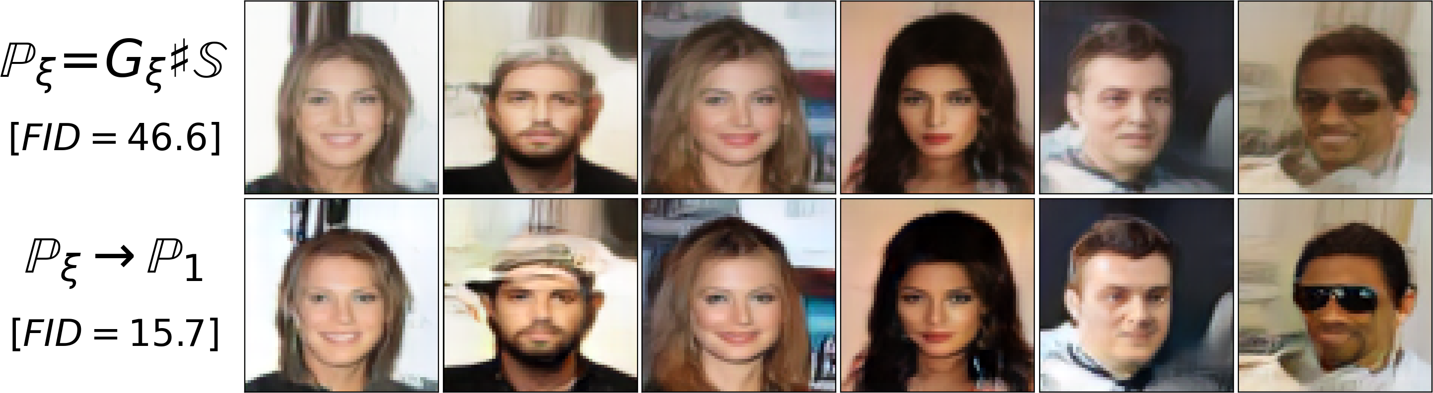
(a) Generator $G_{\xi}$ training enabled ($K_{G}>0$).

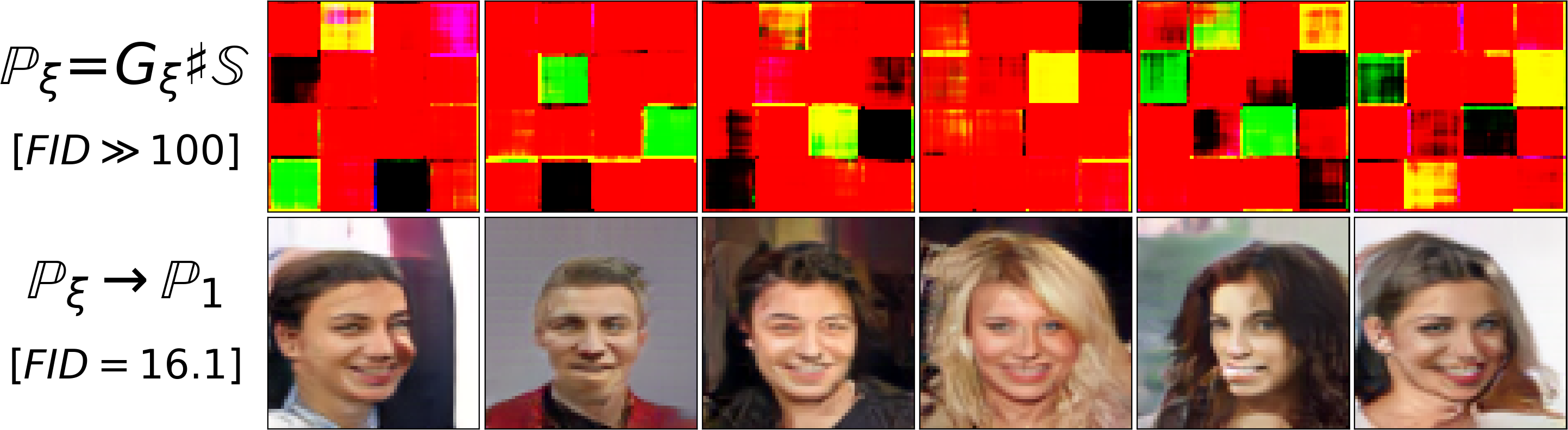
(b) Generator $G_{\xi}$ training disabled ($K_{G}=0$).

Figure 11: Images generated by our algorithm 1 serving as a generative model. The 1st line shows samples from ${G_{\xi}\sharp\mathbb{S}\approx\mathbb{P}_{\text{1}}}$, the 2nd line shows estimated OT map $\widehat{T}_{\mathbb{P}_{\xi}\rightarrow\mathbb{P}_{1}}$ from $G_{\xi}\sharp\mathbb{S}$ to $\mathbb{P}_{1}$ which further improves generated images.

In Table 6, we provide FID for generated images. For comparison, we include FID for ICNN-based $[\text{SC}\mathbb{W}_{2}\text{B}]$, and WGAN-QC [35]. FID scores are adapted from [29, 4.5]. Note that for $N=1$, $[\text{SC}\mathbb{W}_{2}\text{B}]$ is reduced to the OT solver by [40] used as the loss for generative models, a setup tested in [29, Figure 3a]. Serving as a generative model when $N=1$, our algorithm 1 performs comparably to WGAN-QC and drastically outperforms ICNN-based $[\text{SC}\mathbb{W}_{2}\text{B}]$.

Method		FID$\downarrow$
$[\text{SC}\mathbb{W}_{2}B]$	$G_{\xi}(z)$	90.2
	$\widehat{T}_{\mathbb{P}_{\xi}\rightarrow\mathbb{P}_{1}}\big{(}G_{\xi}(z)\big{)}$	89.8
WGAN-QC	$G_{\xi}(z)$	14.4
Ours	$G_{\xi}(z)$	46.6
	$\widehat{T}_{\mathbb{P}_{\xi}\rightarrow\mathbb{P}_{1}}\big{(}G_{\xi}(z)\big{)}$	15.7
Ours (fixed $G_{\xi}$)	$G_{\xi}(z)$	N/A
	$\widehat{T}_{\mathbb{P}_{\xi}\rightarrow\mathbb{P}_{1}}\big{(}G_{\xi}(z)\big{)}$	16.1

Table 6: FID scores of generated faces.

Fixed generator. For $N\!=\!1$, the fixed point approach 4.1 converges in only one step since operator $\mathcal{H}$ immediately maps $G_{\xi}\sharp\mathbb{S}$ to $\mathbb{P}_{1}$. As a result, in our algorithm 1, exclusively when $N=1$, we can fix generator $G_{\xi}$ and train only OT map $T_{\theta_{1}}$ from $G_{\xi}\sharp\mathbb{S}$ to data measure $\mathbb{P}_{1}$ and related potential $v_{\omega_{1}}$. As a sanity check, we conduct such an experiment with randomly initialized generator network $G_{\xi}$. The results are given in Figure 11(b), the FID is included in Table 6. Our algorithm performs well even without generator training at all.

C.4 Barycenters of MNIST Digits and FashionMNIST Classes

Similar to [19, Figure 6], we provide qualitative results of our algorithm applied to computing the barycenter of two MNIST classes of digits $0,1$. The barycenter w.r.t. weights $(\frac{1}{2},\frac{1}{2})$ computed by our algorithm is shown in Figure 12. We also consider a more complex FashionMNIST [66] dataset. Here we compute the barycenter of 10 classes w.r.t. weights $(\frac{1}{10},\dots,\frac{1}{10})$. The results are given in Figures 13 and Figure 14.

Due to (6), each barycenter images are an average (in pixel space) of certain images from the input measure. In all the Figures, the produced barycenter images satisfy this property. The maps to input measures are visually good. The approximate fixed point operator $\mathcal{H}(\mathbb{P}_{\xi})$ is almost the identity as expected (the method converged).

C.5 Additional Results

In Figure 16, we visualize maps between Ave, Celeba! subsets through the learned barycenter. In Figure 15, we provide additional qualitative results for computing barycenters of Handbags, Shoes, Fruit360 datasets.

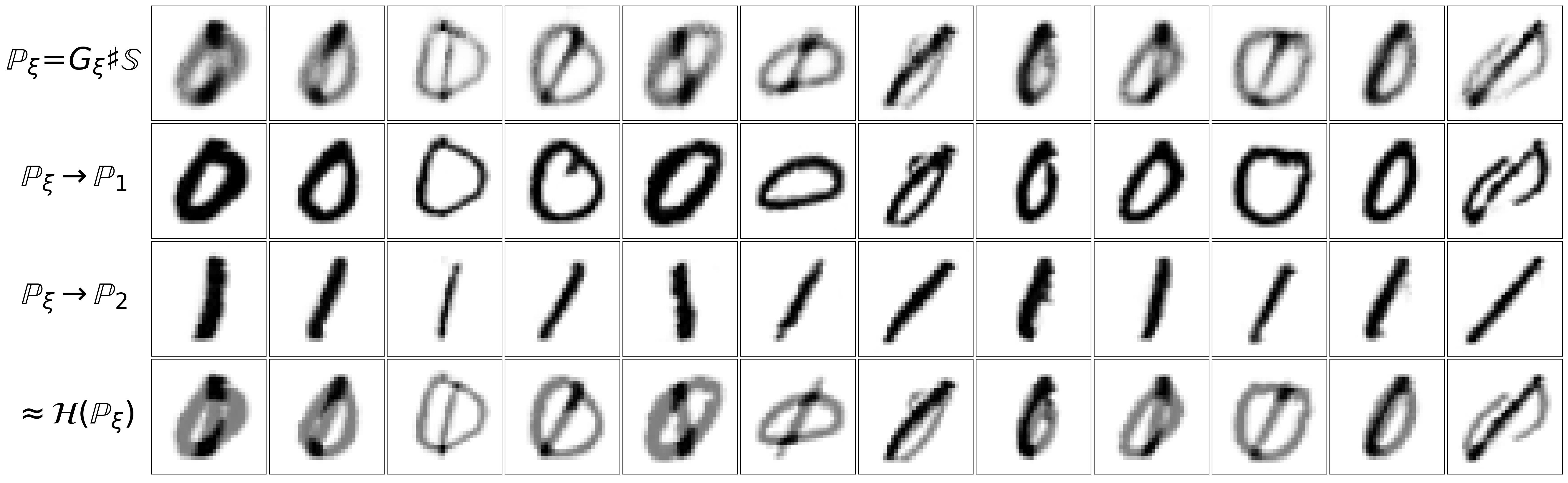
(a) The barycenter $\mathbb{P}_{\xi}$ and maps to input measures $\mathbb{P}_{n}$.

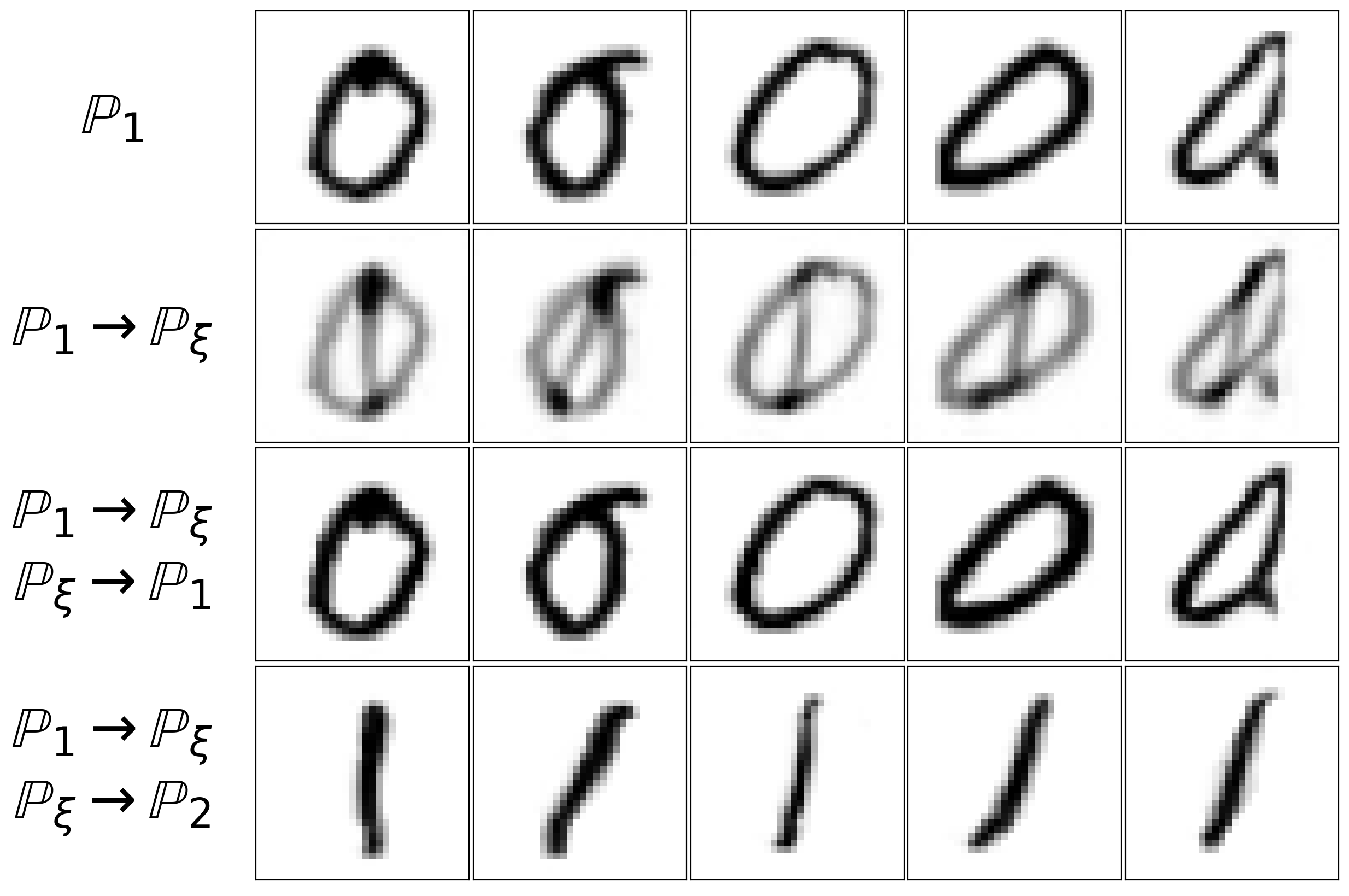
(b) Samples from $\mathbb{P}_{1}$ mapped through $\mathbb{P}_{\xi}$ to each $\mathbb{P}_{n}$.

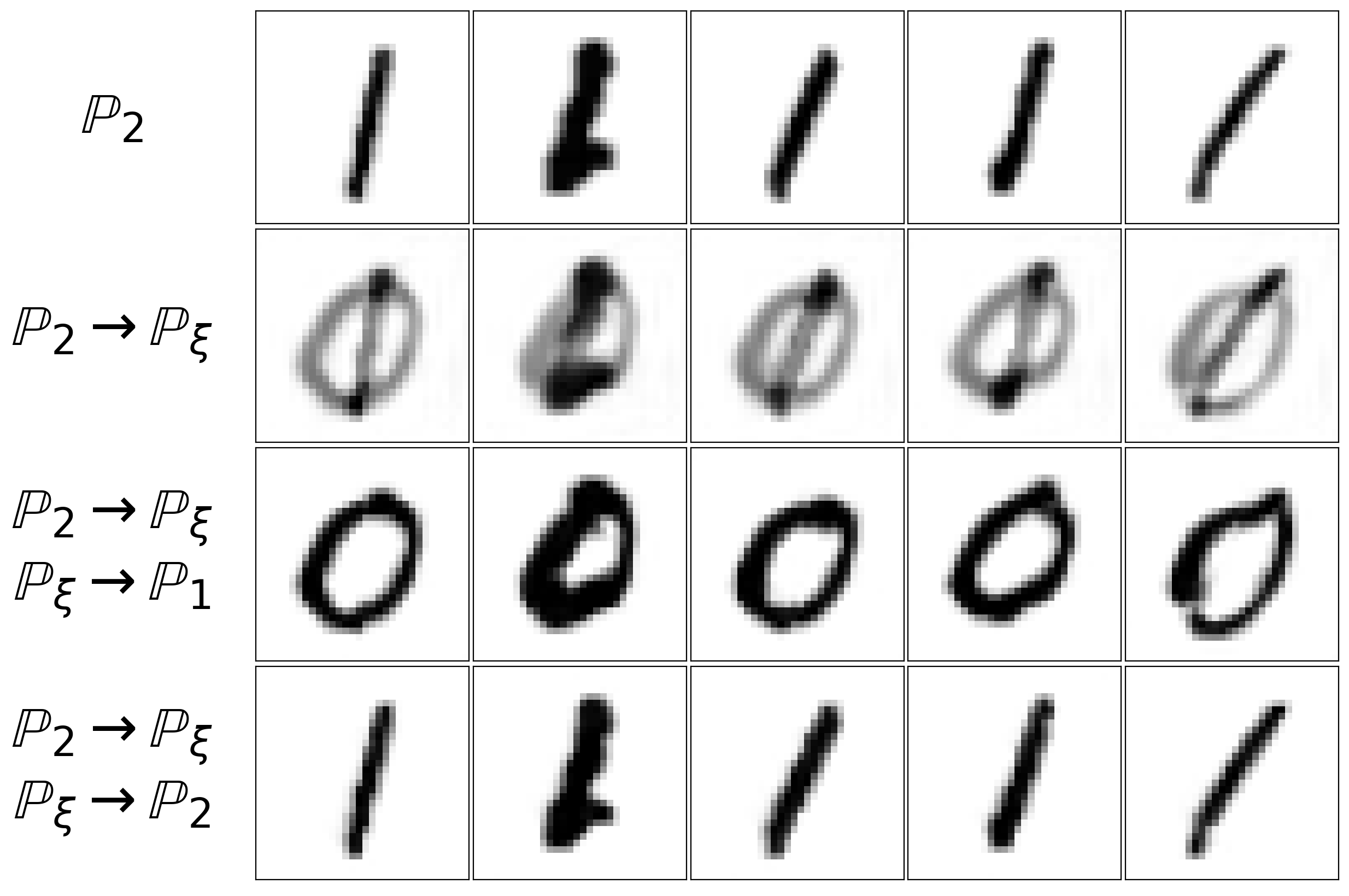
(c) Samples from $\mathbb{P}_{2}$ mapped through $\mathbb{P}_{\xi}$ to each $\mathbb{P}_{n}$.

Figure 12: The barycenter of MNIST digit classes 0/1 learned by Algorithm 1.

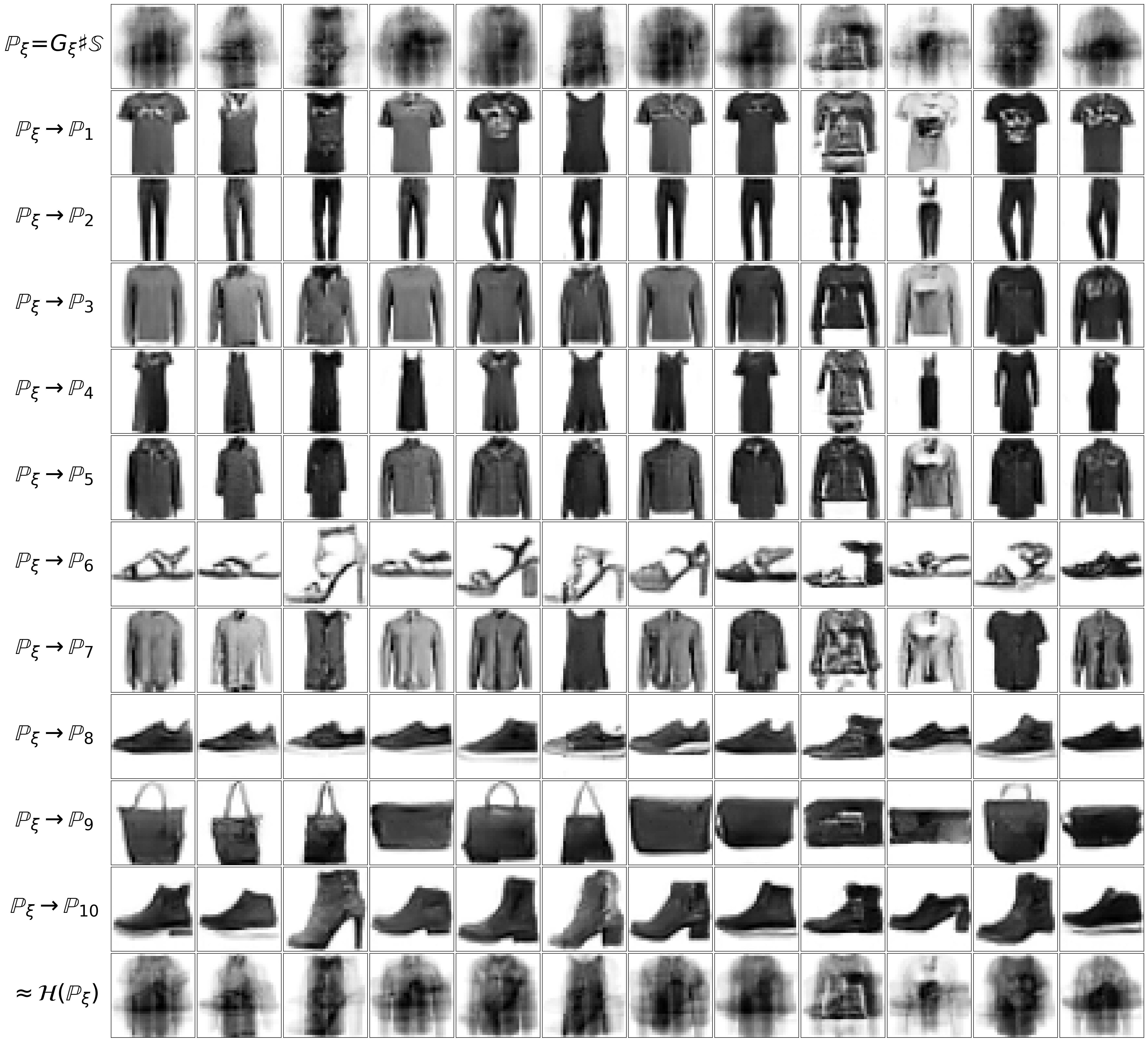
Figure 13: The barycenter and maps to input measures estimated by our method on 10 FashionMNIST classes (32$\times$32). The 1st line shows generated samples from $\mathbb{P}_{\xi}=G_{\xi}\sharp\mathbb{S}\approx\overline{\mathbb{P}}$. Each of 10 next lines shows estimated optimal maps $\widehat{T}_{\mathbb{P}_{\xi}\rightarrow\mathbb{P}_{n}}$ to measures $\mathbb{P}_{n}$. The last line shows average $\big{[}\sum_{n=1}^{N}\alpha_{n}\widehat{T}_{\mathbb{P}_{\xi}\rightarrow\mathbb{P}_{n}}\big{]}\sharp\mathbb{P}_{\xi}$.

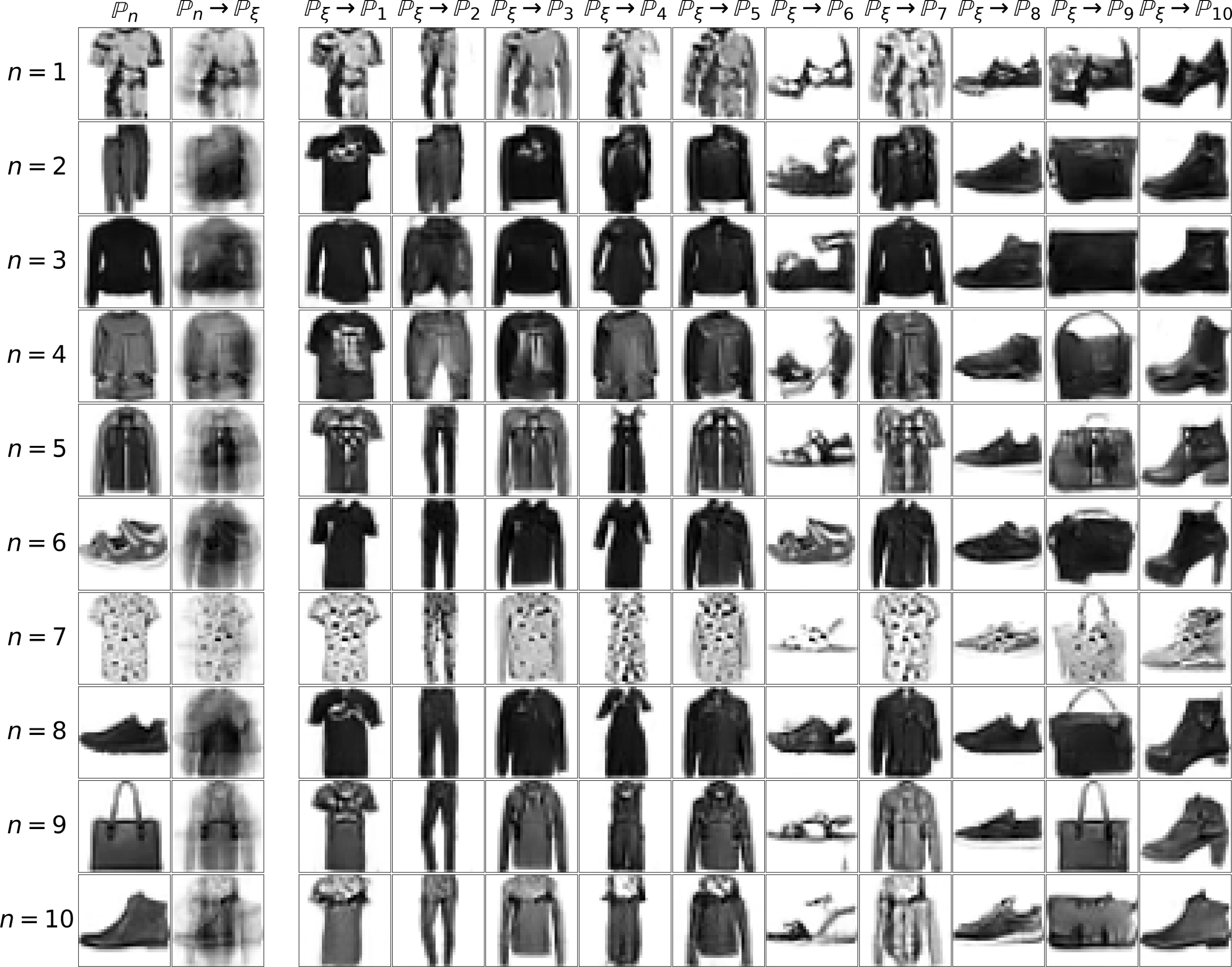
Figure 14: Maps between FashionMNIST classes through the learned barycenter. The 1st images in each $n$-th column shows a sample from $\mathbb{P}_{n}$. The 2nd columns maps these samples to the barycenter. Each next column shows how the maps from the barycenter to the input classes $\mathbb{P}_{n}$.

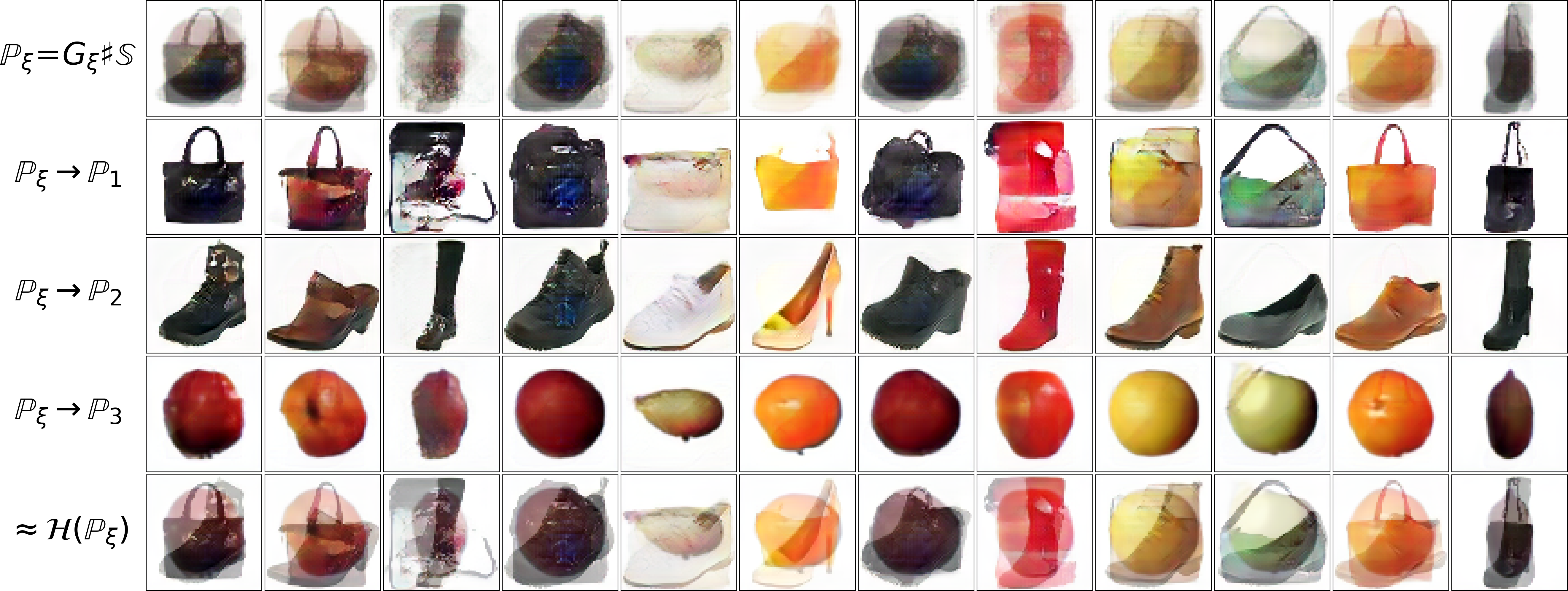
(a) Generated samples $\mathbb{P}_{\xi}\approx\overline{\mathbb{P}}$, fitted maps to each $\mathbb{P}_{n}$ and their average.

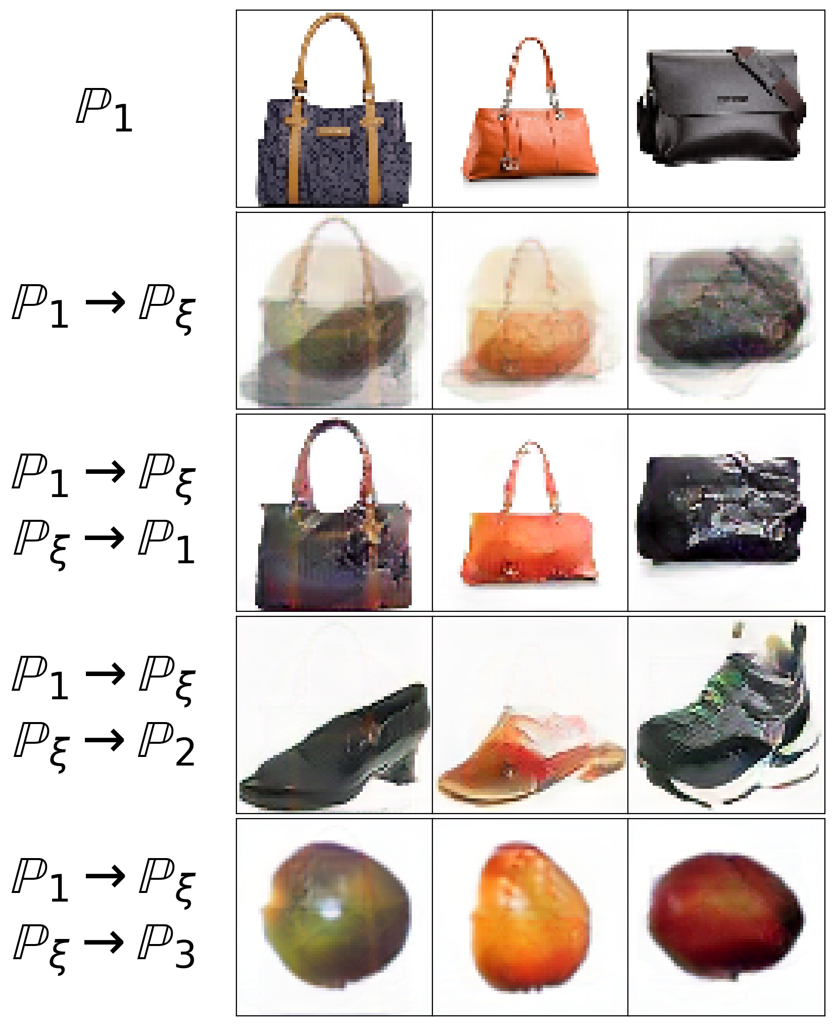
(b) Samples $y\sim\mathbb{P}_{1}$ mapped through $\mathbb{P}_{\xi}$ to each $\mathbb{P}_{n}$.

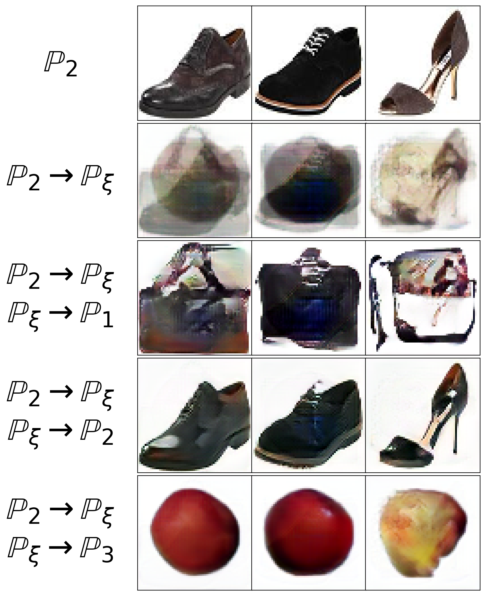
(c) Samples $y\sim\mathbb{P}_{2}$ mapped through $\mathbb{P}_{\xi}$ to each $\mathbb{P}_{n}$.

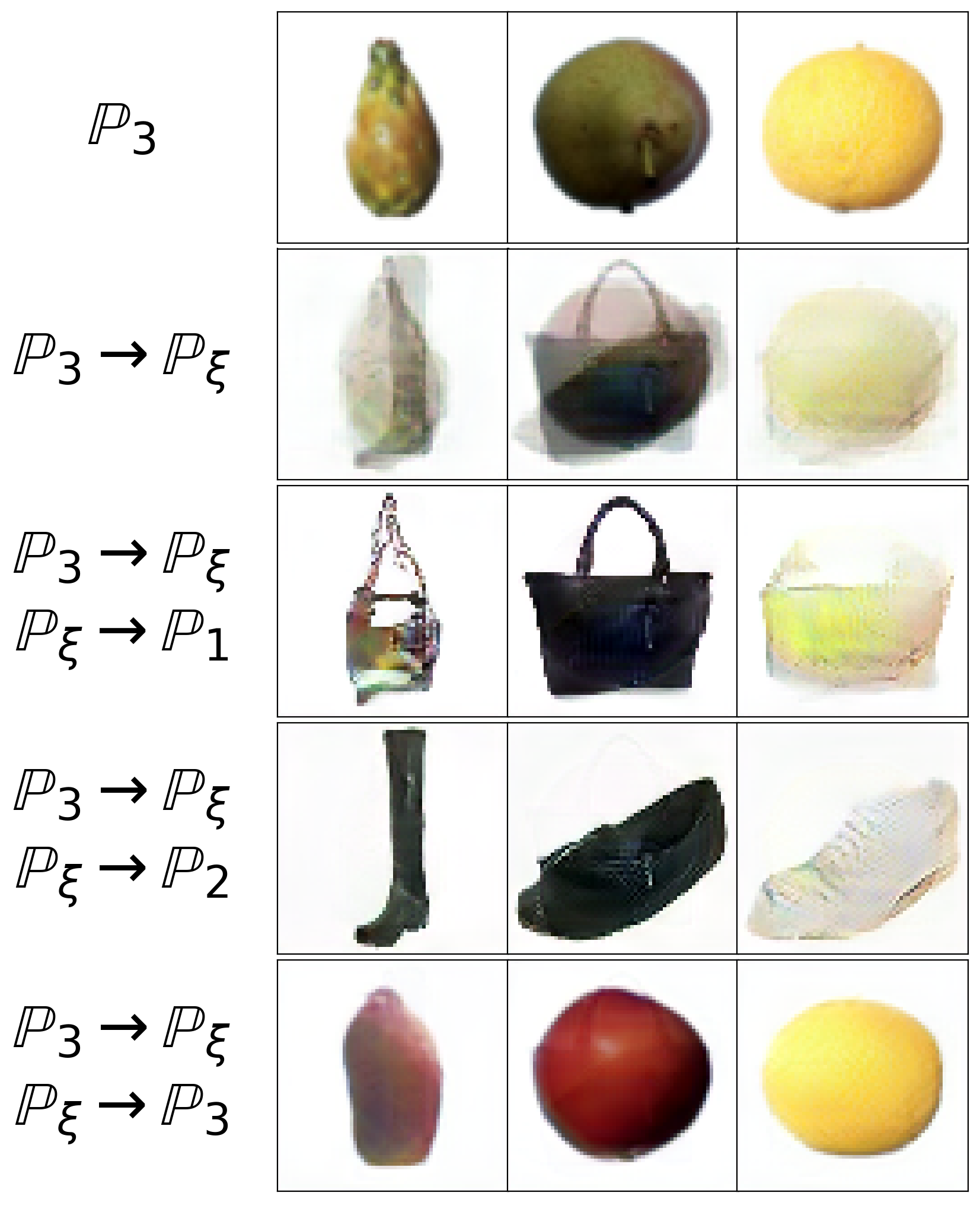
(d) Samples $y\sim\mathbb{P}_{3}$ mapped through $\mathbb{P}_{\xi}$ to each $\mathbb{P}_{n}$.

Figure 15: The barycenter of Handbags, Shoes, Fruit ($64\times 64$) datasets fitted by our algorithm 1.

(a) Samples $y\sim\mathbb{P}_{1}$ mapped through $\mathbb{P}_{\xi}$ to each $\mathbb{P}_{n}$.

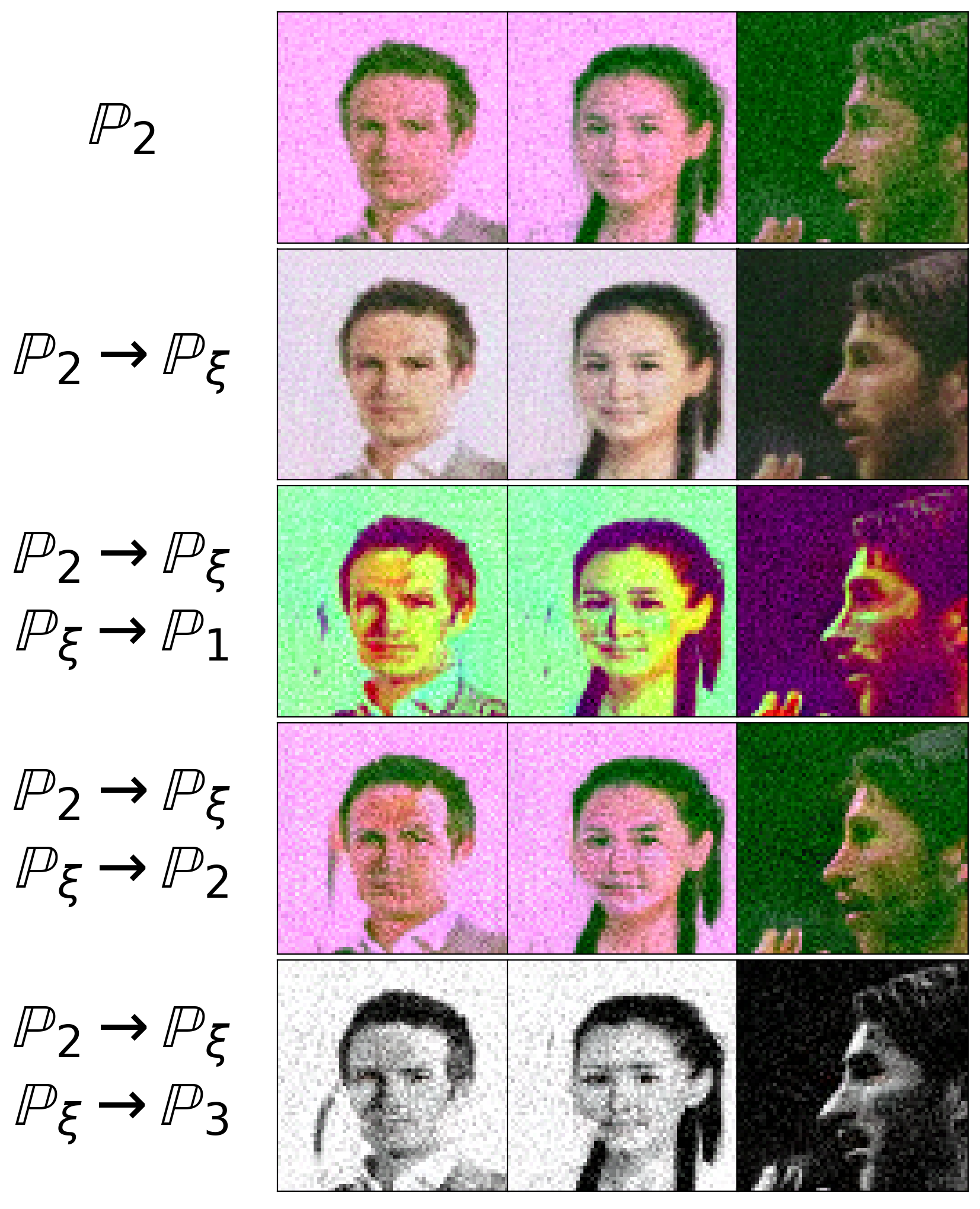
(b) Samples $y\sim\mathbb{P}_{2}$ mapped through $\mathbb{P}_{\xi}$ to each $\mathbb{P}_{n}$.

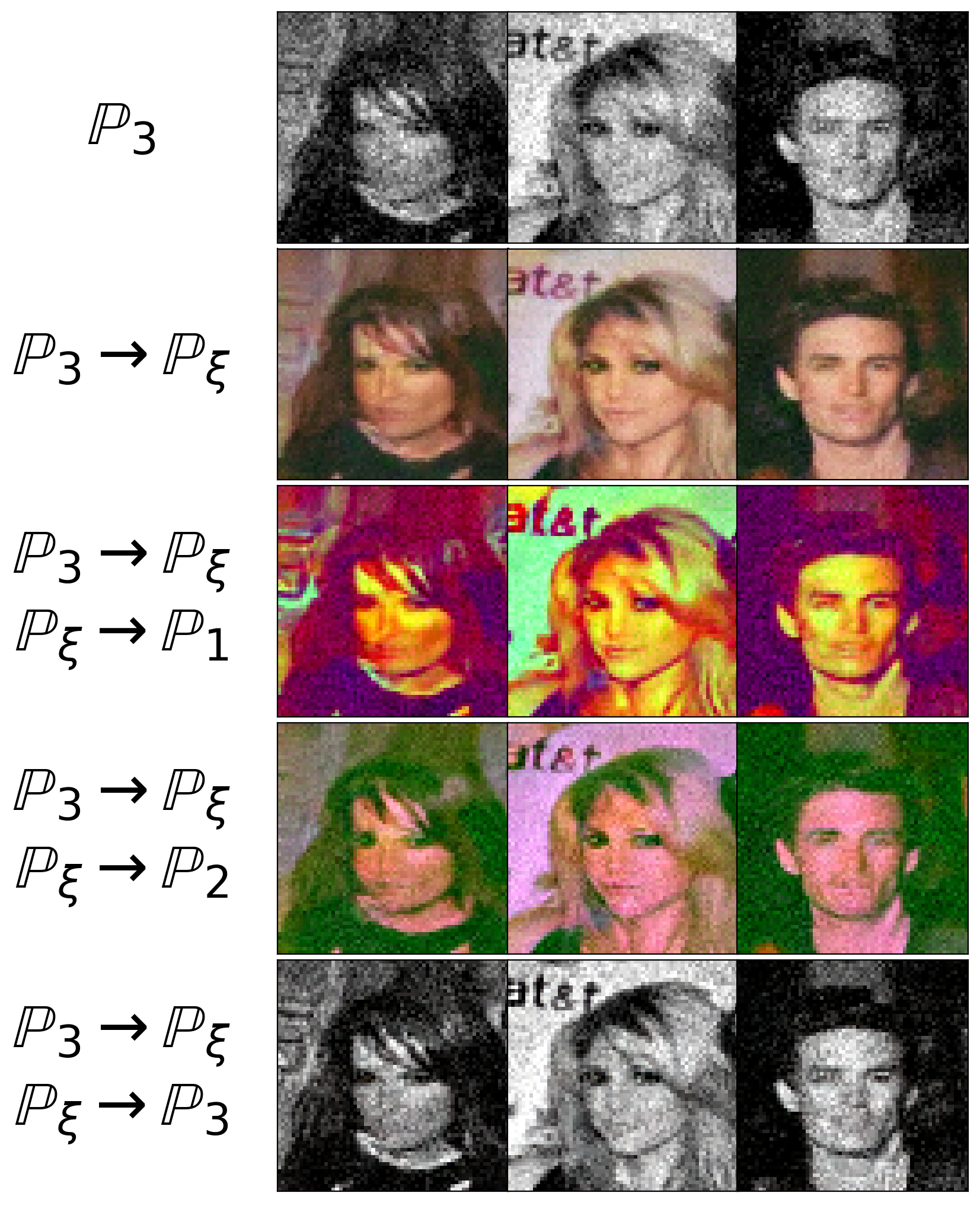
(c) Samples $y\sim\mathbb{P}_{3}$ mapped through $\mathbb{P}_{\xi}$ to each $\mathbb{P}_{n}$.

Figure 16: Maps between subsets of Ave, celeba! dataset through the barycenter learned by our algorithm 1.

References

- [1] Martial Agueh and Guillaume Carlier. Barycenters in the Wasserstein space. SIAM Journal on Mathematical Analysis, 43(2):904–924, 2011.
- [2] Jason M Altschuler, Sinho Chewi, Patrik Gerber, and Austin J Stromme. Averaging on the bures-wasserstein manifold: dimension-free convergence of gradient descent. arXiv preprint arXiv:2106.08502, 2021.
- [3] Pedro C Álvarez-Esteban, E Del Barrio, JA Cuesta-Albertos, and C Matrán. A fixed-point approach to barycenters in Wasserstein space. Journal of Mathematical Analysis and Applications, 441(2):744–762, 2016.
- [4] Brandon Amos, Lei Xu, and J Zico Kolter. Input convex neural networks. In Proceedings of the 34th International Conference on Machine Learning-Volume 70, pages 146–155. JMLR. org, 2017.
- [5] Martin Arjovsky, Soumith Chintala, and Léon Bottou. Wasserstein GAN. arXiv preprint arXiv:1701.07875, 2017.
- [6] Serguei Barannikov, Ilya Trofimov, Nikita Balabin, and Evgeny Burnaev. Representation topology divergence: A method for comparing neural network representations. In Kamalika Chaudhuri, Stefanie Jegelka, Le Song, Csaba Szepesvari, Gang Niu, and Sivan Sabato, editors, Proceedings of the 39th International Conference on Machine Learning, volume 162 of Proceedings of Machine Learning Research, pages 1607–1626. PMLR, 17–23 Jul 2022.
- [7] Serguei Barannikov, Ilya Trofimov, Grigorii Sotnikov, Ekaterina Trimbach, Alexander Korotin, Alexander Filippov, and Evgeny Burnaev. Manifold topology divergence: a framework for comparing data manifolds. Advances in Neural Information Processing Systems, 34:7294–7305, 2021.
- [8] Iaroslav Bespalov, Nazar Buzun, Oleg Kachan, and Dmitry V Dylov. Data augmentation with manifold barycenters. arXiv preprint arXiv:2104.00925, 2021.
- [9] Jérémie Bigot, Elsa Cazelles, and Nicolas Papadakis. Data-driven regularization of wasserstein barycenters with an application to multivariate density registration. Information and Inference: A Journal of the IMA, 8(4):719–755, 2019.
- [10] Nicolas Bonneel, Julien Rabin, Gabriel Peyré, and Hanspeter Pfister. Sliced and radon wasserstein barycenters of measures. Journal of Mathematical Imaging and Vision, 51(1):22–45, 2015.
- [11] Yann Brenier. Polar factorization and monotone rearrangement of vector-valued functions. Communications on pure and applied mathematics, 44(4):375–417, 1991.
- [12] Yucheng Chen, Matus Telgarsky, Chao Zhang, Bolton Bailey, Daniel Hsu, and Jian Peng. A gradual, semi-discrete approach to generative network training via explicit Wasserstein minimization. In International Conference on Machine Learning, pages 1071–1080. PMLR, 2019.
- [13] Sinho Chewi, Tyler Maunu, Philippe Rigollet, and Austin J Stromme. Gradient descent algorithms for bures-wasserstein barycenters. In Conference on Learning Theory, pages 1276–1304. PMLR, 2020.
- [14] Jinjin Chi, Zhiyao Yang, Jihong Ouyang, and Ximing Li. Variational wasserstein barycenters with c-cyclical monotonicity. arXiv preprint arXiv:2110.11707, 2021.
- [15] Pierre Colombo, Guillaume Staerman, Chloe Clavel, and Pablo Piantanida. Automatic text evaluation through the lens of wasserstein barycenters, 2021.
- [16] Chiheb Daaloul, Thibaut Le Gouic, Jacques Liandrat, and Magali Tournus. Sampling from the wasserstein barycenter. arXiv preprint arXiv:2105.01706, 2021.
- [17] Pierre Dognin, Igor Melnyk, Youssef Mroueh, Jerret Ross, Cicero Dos Santos, and Tom Sercu. Wasserstein barycenter model ensembling. arXiv preprint arXiv:1902.04999, 2019.
- [18] Christian Etmann, Rihuan Ke, and Carola-Bibiane Schönlieb. iunets: learnable invertible up-and downsampling for large-scale inverse problems. In 2020 IEEE 30th International Workshop on Machine Learning for Signal Processing (MLSP), pages 1–6. IEEE, 2020.
- [19] Jiaojiao Fan, Amirhossein Taghvaei, and Yongxin Chen. Scalable computations of Wasserstein barycenter via input convex neural networks. arXiv preprint arXiv:2007.04462, 2020.
- [20] Werner Fenchel. On conjugate convex functions. Canadian Journal of Mathematics, 1(1):73–77, 1949.
- [21] Aude Genevay, Marco Cuturi, Gabriel Peyré, and Francis Bach. Stochastic optimization for large-scale optimal transport. In Advances in neural information processing systems, pages 3440–3448, 2016.
- [22] Aude Genevay, Gabriel Peyré, and Marco Cuturi. Gan and vae from an optimal transport point of view. arXiv preprint arXiv:1706.01807, 2017.
- [23] Martin Heusel, Hubert Ramsauer, Thomas Unterthiner, Bernhard Nessler, and Sepp Hochreiter. GANs trained by a two time-scale update rule converge to a local nash equilibrium. In Advances in neural information processing systems, pages 6626–6637, 2017.
- [24] David I Inouye, Zeyu Zhou, Ziyu Gong, and Pradeep Ravikumar. Iterative barycenter flows. arXiv preprint arXiv:2104.07232, 2021.
- [25] Leonid Kantorovitch. On the translocation of masses. Management Science, 5(1):1–4, 1958.
- [26] Diederik P Kingma and Jimmy Ba. Adam: A method for stochastic optimization. arXiv preprint arXiv:1412.6980, 2014.
- [27] Diana Koldasbayeva, Polina Tregubova, Dmitrii Shadrin, Mikhail Gasanov, and Maria Pukalchik. Large-scale forecasting of heracleum sosnowskyi habitat suitability under the climate change on publicly available data. Scientific reports, 12(1):1–11, 2022.
- [28] Alexander Korotin, Vage Egiazarian, Arip Asadulaev, Alexander Safin, and Evgeny Burnaev. Wasserstein-2 generative networks. In International Conference on Learning Representations, 2021.
- [29] Alexander Korotin, Lingxiao Li, Aude Genevay, Justin M Solomon, Alexander Filippov, and Evgeny Burnaev. Do neural optimal transport solvers work? a continuous wasserstein-2 benchmark. Advances in Neural Information Processing Systems, 34:14593–14605, 2021.
- [30] Alexander Korotin, Lingxiao Li, Justin Solomon, and Evgeny Burnaev. Continuous wasserstein-2 barycenter estimation without minimax optimization. In International Conference on Learning Representations, 2021.
- [31] Alexander Korotin, Vladimir V’yugin, and Evgeny Burnaev. Mixability of integral losses: A key to efficient online aggregation of functional and probabilistic forecasts. Pattern Recognition, 120:108175, 2021.
- [32] Julien Lacombe, Julie Digne, Nicolas Courty, and Nicolas Bonneel. Learning to generate wasserstein barycenters. arXiv preprint arXiv:2102.12178, 2021.
- [33] Yann LeCun and Corinna Cortes. MNIST handwritten digit database. 2010.
- [34] Lingxiao Li, Aude Genevay, Mikhail Yurochkin, and Justin Solomon. Continuous regularized Wasserstein barycenters. arXiv preprint arXiv:2008.12534, 2020.
- [35] Huidong Liu, Xianfeng Gu, and Dimitris Samaras. Wasserstein GAN with quadratic transport cost. In Proceedings of the IEEE International Conference on Computer Vision, pages 4832–4841, 2019.
- [36] Ziwei Liu, Ping Luo, Xiaogang Wang, and Xiaoou Tang. Deep learning face attributes in the wild. In Proceedings of International Conference on Computer Vision (ICCV), December 2015.
- [37] Guansong Lu, Zhiming Zhou, Jian Shen, Cheng Chen, Weinan Zhang, and Yong Yu. Large-scale optimal transport via adversarial training with cycle-consistency. arXiv preprint arXiv:2003.06635, 2020.
- [38] Mario Lucic, Karol Kurach, Marcin Michalski, Sylvain Gelly, and Olivier Bousquet. Are GANs created equal? a large-scale study. In Advances in neural information processing systems, pages 700–709, 2018.
- [39] Boyang Lyu, Thuan Nguyen, Prakash Ishwar, Matthias Scheutz, and Shuchin Aeron. Barycenteric distribution alignment and manifold-restricted invertibility for domain generalization, 2021.
- [40] Ashok Vardhan Makkuva, Amirhossein Taghvaei, Sewoong Oh, and Jason D Lee. Optimal transport mapping via input convex neural networks. arXiv preprint arXiv:1908.10962, 2019.
- [41] Alberto Maria Metelli, Amarildo Likmeta, and Marcello Restelli. Propagating uncertainty in reinforcement learning via wasserstein barycenters. In 33rd Conference on Neural Information Processing Systems, NeurIPS 2019, pages 4335–4347. Curran Associates, Inc., 2019.
- [42] Petr Mokrov, Alexander Korotin, Lingxiao Li, Aude Genevay, Justin M Solomon, and Evgeny Burnaev. Large-scale wasserstein gradient flows. Advances in Neural Information Processing Systems, 34:15243–15256, 2021.
- [43] Eduardo Fernandes Montesuma and Fred Maurice Ngole Mboula. Wasserstein barycenter for multi-source domain adaptation. In Proceedings of the IEEE/CVF Conference on Computer Vision and Pattern Recognition, pages 16785–16793, 2021.
- [44] Youssef Mroueh. Wasserstein style transfer. arXiv preprint arXiv:1905.12828, 2019.
- [45] Horea Mureşan and Mihai Oltean. Fruit recognition from images using deep learning. arXiv preprint arXiv:1712.00580, 2017.
- [46] Quan Hoang Nhan Dam, Trung Le, Tu Dinh Nguyen, Hung Bui, and Dinh Phung. Threeplayer Wasserstein GAN via amortised duality. In Proc. of the 28th Int. Joint Conf. on Artificial Intelligence (IJCAI), 2019.
- [47] Quentin Paris. Online learning with exponential weights in metric spaces. arXiv preprint arXiv:2103.14389, 2021.
- [48] Gabriel Peyré, Marco Cuturi, et al. Computational optimal transport. Foundations and Trends® in Machine Learning, 11(5-6):355–607, 2019.
- [49] Julien Rabin, Sira Ferradans, and Nicolas Papadakis. Adaptive color transfer with relaxed optimal transport. In 2014 IEEE International Conference on Image Processing (ICIP), pages 4852–4856. IEEE, 2014.
- [50] Julien Rabin, Gabriel Peyré, Julie Delon, and Marc Bernot. Wasserstein barycenter and its application to texture mixing. In International Conference on Scale Space and Variational Methods in Computer Vision, pages 435–446. Springer, 2011.
- [51] R Tyrrell Rockafellar. Integral functionals, normal integrands and measurable selections. In Nonlinear operators and the calculus of variations, pages 157–207. Springer, 1976.
- [52] Olaf Ronneberger, Philipp Fischer, and Thomas Brox. U-net: Convolutional networks for biomedical image segmentation. In International Conference on Medical image computing and computer-assisted intervention, pages 234–241. Springer, 2015.
- [53] Litu Rout, Alexander Korotin, and Evgeny Burnaev. Generative modeling with optimal transport maps. In International Conference on Learning Representations, 2021.
- [54] Filippo Santambrogio. Optimal transport for applied mathematicians. Birkäuser, NY, 55(58-63):94, 2015.
- [55] Vivien Seguy, Bharath Bhushan Damodaran, Rémi Flamary, Nicolas Courty, Antoine Rolet, and Mathieu Blondel. Large-scale optimal transport and mapping estimation. arXiv preprint arXiv:1711.02283, 2017.
- [56] Dror Simon and Aviad Aberdam. Barycenters of natural images constrained wasserstein barycenters for image morphing. In Proceedings of the IEEE/CVF Conference on Computer Vision and Pattern Recognition, pages 7910–7919, 2020.
- [57] Karen Simonyan and Andrew Zisserman. Very deep convolutional networks for large-scale image recognition. arXiv preprint arXiv:1409.1556, 2014.
- [58] Justin Solomon, Fernando De Goes, Gabriel Peyré, Marco Cuturi, Adrian Butscher, Andy Nguyen, Tao Du, and Leonidas Guibas. Convolutional Wasserstein distances: Efficient optimal transportation on geometric domains. ACM Transactions on Graphics (TOG), 34(4):1–11, 2015.
- [59] Sanvesh Srivastava, Volkan Cevher, Quoc Dinh, and David Dunson. Wasp: Scalable bayes via barycenters of subset posteriors. In Artificial Intelligence and Statistics, pages 912–920, 2015.
- [60] Sanvesh Srivastava, Cheng Li, and David B Dunson. Scalable bayes via barycenter in Wasserstein space. The Journal of Machine Learning Research, 19(1):312–346, 2018.
- [61] Thomas Staudt, Shayan Hundrieser, and Axel Munk. On the uniqueness of kantorovich potentials. arXiv preprint arXiv:2201.08316, 2022.
- [62] Amirhossein Taghvaei and Amin Jalali. 2-Wasserstein approximation via restricted convex potentials with application to improved training for GANs. arXiv preprint arXiv:1902.07197, 2019.
- [63] Jules Vidal, Joseph Budin, and Julien Tierny. Progressive wasserstein barycenters of persistence diagrams. IEEE transactions on visualization and computer graphics, 26(1):151–161, 2019.
- [64] Cédric Villani. Topics in optimal transportation. Number 58. American Mathematical Soc., 2003.
- [65] Cédric Villani. Optimal transport: old and new, volume 338. Springer Science & Business Media, 2008.
- [66] Han Xiao, Kashif Rasul, and Roland Vollgraf. Fashion-mnist: a novel image dataset for benchmarking machine learning algorithms. arXiv preprint arXiv:1708.07747, 2017.
- [67] Yujia Xie, Minshuo Chen, Haoming Jiang, Tuo Zhao, and Hongyuan Zha. On scalable and efficient computation of large scale optimal transport. volume 97 of Proceedings of Machine Learning Research, pages 6882–6892, Long Beach, California, USA, 09–15 Jun 2019. PMLR.
- [68] Aron Yu and Kristen Grauman. Fine-grained visual comparisons with local learning. In Proceedings of the IEEE Conference on Computer Vision and Pattern Recognition, pages 192–199, 2014.