Joint Differential Optimization and Verification for Certified Reinforcement Learning

Abstract.

Model-based reinforcement learning has been widely studied for controller synthesis in cyber-physical systems (CPSs). In particular, for safety-critical CPSs, it is important to formally certify system properties (e.g., safety, stability) under the learned RL controller. However, as existing methods typically conduct formal verification after the controller has been learned, it is often difficult to obtain any certificate, even after many iterations between learning and verification. To address this challenge, we propose a framework that jointly conducts reinforcement learning and formal verification by formulating and solving a novel bilevel optimization problem, which is end-to-end differentiable by the gradients from the value function and certificates formulated by linear programs and semi-definite programs. In experiments, our framework is compared with a baseline model-based stochastic value gradient (SVG) method and its extension to solve constrained Markov Decision Processes (CMDPs) for safety. The results demonstrate the significant advantages of our framework in finding feasible controllers with certificates, i.e., barrier functions and Lyapunov functions that formally ensure system safety and stability.

1. Introduction

Applying machine learning techniques in cyber-physical systems (CPSs) has attracted much attention. In particular, reinforcement learning (RL) has shown great promise (Wang et al., 2021), such as in robotics (Koch et al., 2019) and smart buildings (Xu et al., 2020; Wei et al., 2017), where RL trains control policy by maximizing the value function of the goal state (Sutton and Barto, 2018). However, there is still significant hesitation in applying RL to safety-critical applications (Knight, 2002; Zhu and Sangiovanni-Vincentelli, 2018) of CPSs, such as in autonomous vehicles (Liu et al., 2022, 2023; Wang et al., 2022a), because of the uncertain and potentially dangerous impact on system safety (Wang et al., 2020; Zhu et al., 2021, 2020). It is thus important to find RL-learned controllers that are certified, i.e., under which critical system properties such as safety and stability can be formally guaranteed. And a common approach to guarantee these properties is to find corresponding certificates for them, e.g., a barrier function for safety (Prajna and Jadbabaie, 2004) and a Lyapunov function for stability (Lyapunov, 1992).

In this work, we focus particularly on learning certified controllers with RL for CPSs that can be modeled as ordinary differential equations (ODEs) with unknown parameters, a common scenario in practice. Traditionally, this is typically done in a two-step ‘open-loop’ process: 1) first, model-based reinforcement learning (MBRL) is conducted to learn the system model parameters and the controller simultaneously, and then 2) based on the identified dynamics, formal verification is performed to find certificates for various system properties by solving optimization problems. However, with such an open-loop paradigm, it is often difficult to find any feasible certificates even after many iterations of learning and verification steps, and the failed verification results are not leveraged sufficiently in the learning of a new controller. Thus, integrating controller synthesis and certificate generation in a more holistic manner has received increasing attention recently.

Pioneering works on control-certificate joint learning mainly focus on systems with known models, i.e., explicit models without any unknown parameters (Qin et al., 2021; Wang et al., 2022b; Luo and Ma, 2021; Tsukamoto and Chung, 2020; Robey et al., 2020; Lindemann et al., 2021; Dawson et al., 2022b; Chang et al., 2019). Those methods typically collect samples from the system space, transform the certificate conditions into loss functions, and solve them via supervised learning methods. However, they cannot be directly used to address systems with unknown parameters, and the certificates obtained in those works are often tested/validated via sampling-based approaches without being formally verified.

Moreover, for safety properties, methods that are based on solving constrained Markov Decision Processes (CMDPs) are popular in the safe RL literature (Thananjeyan et al., 2021; Srinivasan et al., 2020; Stooke et al., 2020). However, these methods typically try to achieve safety by restricting the expectation of the cumulative cost for the system’s unsafe actions to be under a certain threshold, which can only be regarded as soft safety constraints as the system may still enter the unsafe region.

Contribution of our work: To address these challenges, we propose a certified RL method with joint differentiable optimization and verification for systems with unknown model parameters. As shown in Fig. 1, our approach seamlessly integrates RL optimization and formal verification by formulating and solving a novel bilevel optimization problem, which generates an optimal controller together with its certificates, e.g., barrier functions for safety and/or Lyapunov functions for stability. Different from CMDP-based methods, we address hard safety constraints where the system should never enter an unsafe region.

The upper-level problem in our bilevel optimization tries to learn the controller parameters $\theta$ and the unknown system model parameters $\alpha$ by MBRL; while the lower-level problem tries to verify system properties by searching for feasible certificates via SDP or LP with a slack variable $c$. Note that we propose LP relaxation in addition to SDP because while SDP may be more efficient for low-dimensional/low-degree systems, LP provides better scalability for higher-dimensional systems. When the lower-level problem fails to find any feasible certificate for given $\theta$ and $\alpha$ from the upper-level MBRL problem, it will return the gradient of the slack variable $c$ over the control parameter $\theta$, to guide the exploration of new $\theta$. Our framework is end-to-end fully differentiable by the gradients from the value function in upper MBRL and from the certificates in lower SDP and LP and can be viewed as a ‘closed-loop learning-verification paradigm where the failed verification provides immediate gradient feedback to the controller synthesis. We conducted experiments on linear and non-linear systems with linear and non-linear controller synthesis, demonstrating significant advantages of our approach over model-based stochastic-value gradient (SVG) and its extension to solve CMDPs for safety. Our approach can find certificates for safety and stability in most cases based on identified dynamics and provide better results of those two properties in simulations.

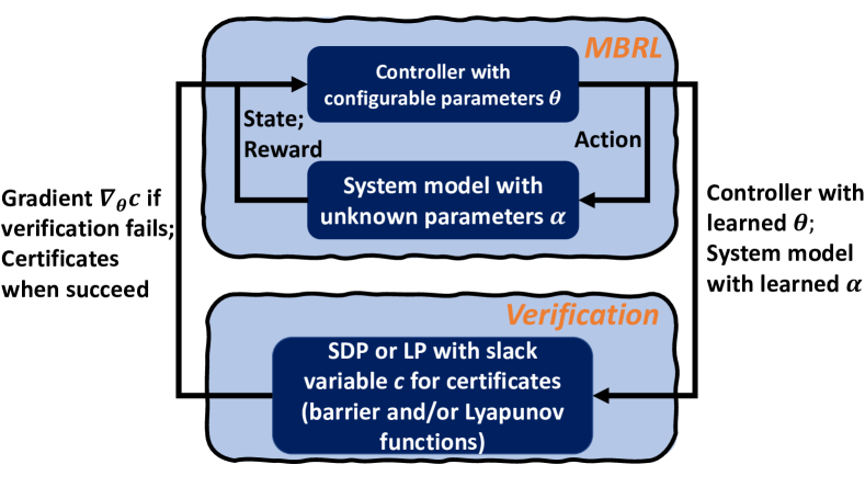
Figure 1. Overview of our joint differentiable optimization and verification framework for certified RL. Our approach integrates RL-based control optimization with formal verification in a closed-loop manner, by formulating and solving a bilevel optimization problem. The upper-level problem learns the controller parameters $\theta$ and the system model parameters $\alpha$ with MBRL, while the lower-level problem verifies system properties by searching for feasible certificates via SDP or LP with a slack variable $c$. The framework is end-to-end differentiable.

In the rest of the paper, Section 2 discusses related works. Section 3 formulates the problem to address. Section 4 presents our proposed approach, and Section 5 shows the experimental results. Section 6 concludes the paper.

2. Related Works

Certificate-based verification in our work is related to the literature on barrier function safety (Prajna and Jadbabaie, 2004) and Lyapunov stability (Lyapunov, 1992), which provide formal guarantees on the safe control of systems to avoid unsafe states and on the system stability around an equilibrium point, respectively. In classical control, finding barrier or Lyapunov functions is challenging (Papachristodoulou and Prajna, 2002) and often requires considerable expertise and manual effort (Chen et al., 2020) through optimization. Our approach, in contrast, automatically searches for certificates and provides gradient feedback from the failed searches to the learning process, to guide the exploration of control parameters for increasing the chance of finding feasible certificates.

Regarding safety in particular, our work aims at addressing hard safety constraints, by ensuring that the system never enters an unsafe region with formal guarantees (Huang et al., 2022, 2019; Fan et al., 2020), both during and after training. In contrast, in the popular CMDP-based methods (Thananjeyan et al., 2021; Srinivasan et al., 2020; Stooke et al., 2020), the agent aims to maximize the expected cumulative reward while restricting the expectation of cumulative cost for their unsafe interactions with the environment under a certain threshold. Since the agent can still take unsafe actions with some cost, the safety constraints in CMDPs can be regarded as addressing soft safety constraints without formal guarantees. There are also works that ensure safety by addressing stability (Berkenkamp et al., 2017) in RL, but we consider these two properties as different in this work, where safety is defined based on the reachability of the system state.

In terms of optimization techniques, our work leverages SVG (Heess et al., 2015) in MBRL and is a first-order, end-to-end differentiable approach with the computation of the analytic gradient of the RL value function. Our work also conducts convex optimization for the certification. As such an optimization problem may not be feasible to solve, our approach tries to ‘repair’ it via a slack variable, which is differentiable to control parameters. This is related to but different from the approach in (Barratt et al., 2021), which tries to repair the infeasible problems by modifying program parameters. Finally, as a differentiable framework, our approach is related to safe PDP (Jin et al., 2021), which, different from ours, requires an explicit dynamical model with no unknown parameters and an initial safe policy.

Our work is also related to the joint learning of controller and verification by leveraging neural networks to represent certificates (Jin et al., 2020; Qin et al., 2021; Luo and Ma, 2021; Tsukamoto and Chung, 2020; Robey et al., 2020; Lindemann et al., 2021; Dawson et al., 2022b; Chang et al., 2019; Robey et al., 2021; Wang et al., 2022c). These approaches first translate the certificate conditions into loss functions, sample and label data points from the system state, and then learn the certificate in a supervised learning manner. However, they require a known system dynamics model or safe demonstration data, and cannot be directly applied to systems models with unknown parameters or without safe data, which is the case our approach addresses via the RL process. Moreover, the neural network-based certificates generated by these approaches are often tested/validated through sampling-based methods and are not formally verified, while our approach provides formal and deterministic guarantees once the certificate is successfully obtained.

3. Problem Formulation

We consider a continuous CPS whose dynamics can be expressed as an ordinary differential equation (ODE):

(1) $$\dot{x}=f(x,u;\alpha),$$

where $x\in X\subset\mathbf{R}^{n}$ is a vector denoting the system state within the state space $X$ and $u\in U\subset\mathbf{R}^{m}$ is the control input variable. $f:\mathbf{R}^{n}\times\mathbf{R}^{m}\rightarrow\mathbf{R}^{n}$ is a locally Lipschitz-continuous function ensuring that there exists a unique solution for the system ODE. Without loss of generality, $f$ is a polynomial function, as common elementary functions, such as $\sin(x),\cos(x),\sqrt{x},\frac{1}{x},e^{x},\ln(x)$ and their combinations, can be equivalently transformed to polynomials (Liu et al., 2015). $\alpha\in\mathbf{R}^{|\alpha|}\in[\underline{\alpha},\bar{\alpha}]$ is a vector denoting the unknown system model parameters, which are within a lower bound $\underline{\alpha}$ and an upper bound $\bar{\alpha}$. The system has an initial state set $X_{0}\subset X$, an unsafe state set $X_{u}\subset X$, and a goal state set $X_{g}\subset X$. Without loss of generality, $X_{g}$ is assumed as the origin point in this paper. These sets are semi-algebraic, which can be expressed as: $X_{0}=\{x|\xi_{i}(x)\geq 0,i=1,\cdots,s\},X_{u}=\{x|\zeta_{i}(x)\geq 0,i=s+1,\cdots,s+q\},X=\{x|\psi_{i}(x)\geq 0,i=s+q+1,\cdots,s+q+r\}.$ The partial derivatives $f_{x}$ and $f_{u}$ can be computed with the parameters $\alpha$. We abbreviate partial differentiation or gradient using subscripts, e.g, $\frac{\partial f(x,u;\alpha)}{\partial x}\overset{\Delta}{=}f_{x}$ with gradient or derivative in front.

Such a continuous system can be controlled by a feedback deterministic controller $\pi(x;\theta)=\theta\cdot w^{\theta}(x):X\rightarrow U$, which is parameterized by vector $\theta\in\mathbb{R}^{|\theta|}$ and monomial basis $w^{\theta}(x)$. Note that $w^{\theta}(x)$ can contains non-linear terms. Given any time $\forall t\geq 0$, the controller $\pi$ reads the system state $x(t)$ at $t$, and computes the control input as $u=\pi(x(t);\theta)$. Overall, the system evolves by following $\dot{x}=f(x,\pi(x;\theta))$ with $\pi$.

A flow function $\varphi(x(0),t):X_{0}\times\mathbb{R}_{+}\rightarrow X$ maps any initial state $x(0)$ to the system state $\varphi(x(0),t)$ at time $t,\forall t\geq 0$. Mathematically, $\varphi$ satisfies 1) $\varphi(x(0),0)=x(0)$, and 2) $\varphi$ is the solution of the $\dot{x}=f(x,u)$. Based on the flow definition, the system safety and stability properties and their corresponding certificates, e.g., barrier function and Lyapunov function, are defined as follows.

Definition 3.1.

(Infinite-time Safety Property) Starting from any initial state $x(0)\in X_{0}$, the system defined in (1) is considered as meeting the safety property if and only if its flow never enters into the unsafe set $X_{u}$: $\forall t\geq 0,\ \varphi(x(0),t)\notin X_{u}.$

This safety property can be formally guaranteed if the controller $\pi$ can obtain a barrier function as:

Definition 3.2.

(Exponential Condition based Barrier Function (Kong et al., 2013)) Given a controller $\pi(x;\theta)$, $B(x;\beta^{B})$ is a safety barrier function parameterized by vector $\beta^{B}\in\mathbb{R}^{|\beta|}$ with $\lambda\in\mathbb{R}$ if:

$$B(x;\beta^{B})\leq 0,\forall x\in X_{0},$$

$$B(x;\beta^{B})>0,\forall x\in X_{u},$$

$$\partialderivative{B}{x}\cdot f(x,\pi(x);\alpha)-\lambda B(x;\beta^{B})\leq 0,\forall x\in X.$$

Remark 3.3.

(Shielding-based One-Step Safety) Another possible way to ensure safety is to check during run-time a pre-defined shield for the system and stop the system when finding a hazard affront. Note that such shielding mechanism is reactional. It tries to protect the system from danger by only looking one step forward, which may degrade the overall performance, as shown in the experiments. Moreover, the system could still be led towards the unsafe region after several steps when taking the current action and has to be stopped eventually. In contrast, if can be found, a barrier function guarantees infinite-time safety.

Definition 3.4.

(Stability Property) Starting from any initial state $x(0)\in X_{0}$, the system defined in (1) is stable around the goal set $X_{g}$ if there exists a $\mathcal{KL}$ function $\tau$ (Khalil, 2002) such that for any $x(0)\in X_{0}$, $\norm{\varphi(x(0),t)}_{X_{g}}\leq\tau(\norm{x(0)}_{X_{g}},t),$ where $\norm{x}_{X_{g}}=\inf_{x_{g}\in X_{g}}\norm{x-x_{g}}$, with $\norm{\cdot}$ denoting the Euclidean distance.

This stability property can be formally guaranteed if there exists a Lyapunov function for $\pi$ as:

Definition 3.5.

(Lyapunov Function) $V(x;\beta^{V})(\beta^{V}\in\mathbb{R}^{|\beta|})$ is a Lyapunov function of controller $\pi(x;\theta)$ if:

$$V(x;\beta^{V})\geq 0,x\in X,$$

$$\partialderivative{V}{x}\cdot f(x,\pi(x;\theta);\alpha)\leq 0,x\in X.$$

Considering the safety and stability certificates, the problem we address in this paper can be defined as a certified control learning problem:

Problem 3.6.

(Certified Control Learning) Given a continuous system defined as in (1), learn the unknown dynamical parameters $\alpha$ and a feedback controller $\pi(x;\theta)$ so that the system formally satisfies the safety property and/or the stability property with barrier function $B(x;\beta^{B})$ and/or Lyapunov function $V(x;\beta^{V})$ as certificates.

4. Our Approach for Certified Differentiable Reinforcement Learning

In this section, we present our certified differentiable reinforcement learning framework to solve the Problem 3.6 defined above. We first introduce a novel bilevel optimization formulation for Problem 3.6 in Section 4.1, by treating the learning of the controller and the system model parameters as an upper-level MBRL problem and formulating the verification as a lower-level SDP or LP problem. We connect these two sub-problems with a slack variable based on certification results. We then solve the bilevel optimization problem with the Algorithm 1 introduced in Section 4.2, which leverages the gradients of the slack variable and the value function in RL, and includes techniques for variable transformation, safety shielding, and parameter identification. Finally, we conduct theoretical analysis on the soundness, incompleteness and optimality of our approach in Section 4.3.

4.1. Bilevel Optimization Problem Formulation

In this section, we introduce a novel and general bilevel optimization problem for the certified control learning framework and then its specific extension to SDP and LP.

In general, we can formulate a constrained optimization problem for the certified control learning defined in Problem 3.6 as:

(2) $$\max_{\theta,\alpha}\mathbb{E}_{f,x(0)\in X_{0}}[\mathcal{V}(x(0))],$$

s.t. $$\mathcal{I}^{i}(x;\theta,\alpha,\beta)\geq 0,$$

$$\mathcal{E}^{j}(x;\theta,\alpha,\beta)=0.$$

Here, $\mathcal{V}(x(0))$ is the value function on the initial state $x(0)\in X_{0}$ in RL. $\mathcal{I}^{i}(x;\theta,\alpha,\beta)$, $\mathcal{E}^{j}(x;\theta,\alpha,\beta)$ are the inequality and equality constraints encoded from barrier certificate and Lyapunov function via various relaxation techniques (such as SDP and LP that are later introduced), with $\theta\in\mathbb{R}^{|\theta|}$, $\alpha\in\mathbb{R}^{|\alpha|}$, $\beta\in\mathbb{R}^{|\beta|}$ as the vector of controller parameters, unknown system parameters, and parameters for certificates, respectively. As RL builds on the discrete-time MDPs, we need to discretize continuous dynamics $f$ to compute $\mathbb{E}[\mathcal{V}(x(0))]$ by simulating different traces with the controller. Specifically, in RL, $\mathcal{V}(x)$ satisfies the Bellman equation as: $\mathcal{V}(x)=r(x,\pi(x))+\gamma\mathcal{V}^{\prime}(x^{\prime}),$ where $r$ is a reward function at the state-action pair $(x,\pi(x))$, encoding the desired learning goal for the controller, $x^{\prime}$ is the next system state, $\mathcal{V}^{\prime}$ is the value function of $x^{\prime}$, and constant factor $\gamma<1$.

Such a constrained optimization problem in RL is often infeasible, where the infeasible certification results cannot directly guide the control learning problem. To leverage the gradient from the verification results and form an end-to-end differentiable framework, the above problem can be modified to our bilevel optimization problem by introducing a slack variable $c\in\mathbb{R}^{+}$. Specifically, the upper problem tries to solve:

$$\max_{\theta,\alpha}\mathbb{E}[\mathcal{V}(x(0);\theta,\alpha)]-\lambda(c^{*}(\theta,\alpha))^{2}-\norm{\alpha-\alpha_{0}}^{2},$$

where $c^{*}(\theta,\alpha)$ is the solution to a lower-level problem:

$$\qquad\min_{\beta}c,~{}$$

(3) subject to $$\begin{cases}\mathcal{I}^{i}(x;\theta,\alpha,\beta)+c\geq 0,\\ \mathcal{E}^{i}(x;\theta,\alpha,\beta)\leq c,\\ \mathcal{E}^{i}(x;\theta,\alpha,\beta)\geq-c,\\ c\geq 0,\end{cases}$$

where $\alpha_{0}\in\mathbb{R}^{|\alpha|}$ is the unknown ground truth value of the unknown system model parameter vector and needs to be estimated in learning. $\lambda\geq 0$ is a penalty multiplier. Overall, the lower-level problem tries to search for a feasible solution for the certificates while reducing the slack variable $c$. The upper-level problem tries to maximize the value function in RL, reduce the penalty from the lower-level slack variable, and learn the uncertain parameters. Once the lower optima $c^{*}=0$, we can obtain a feasible solution for the original constrained problem (2) and therefore generate a certificate. In this way, by differentiating the lower-level problem, the gradient $c^{*}_{\theta}$ of $c^{*}$ with respect to $\theta$ can be combined with the gradient of MBRL in the upper-level problem, and the entire bilevel optimization problem is fully differentiable.

4.1.1. SDP Relaxation for Bilevel Formulation

Definition 4.1.

(Sum-of-Squares) A polynomial $p(x)$ is a sum-of-squares (SOS) if there exist polynomials $f_{1}(x),f_{2}(x),\cdots,f_{m}(x)$ such that $p(x)=\sum_{i=1}^{m}f_{i}(x)^{2}.$ In such case, it is easy to get $p(x)\geq 0$.

For the positivity of SOS, the three conditions in a barrier function as defined in Definition 3.2 can be relaxed into three SOS programmings based on the Putinar’s Positivstellensatz theorem (Nie and Schweighofer, 2007):

$$-B(x)-\sum_{i=1}^{s}\sigma_{i}(x)\cdot\xi_{i}(x)\in\Sigma[x],$$

$$B(x)-\sum_{i=s+1}^{s+q}\sigma_{i}(x)\cdot\zeta_{i}(x)\in\Sigma[x],$$

$$-\partialderivative{B}{x}\cdot f(x,\pi(x))+\lambda B(x)-\sum_{i=s+q+1}^{s+q+r}\sigma_{i}(x)\psi_{i}(x)\in\Sigma[x].$$

Here, $\sigma_{i}\in\Sigma[x]\geq 0,i=1,\cdots,s+q+r$. $\Sigma[x]$ denotes the SOS ring that consists of all the SOSs over $x$. $\xi_{i}(x)\geq 0$, $\zeta_{i}(x)\geq 0$, $\psi_{i}(x)\geq 0$ are the semi-algebraic constraints on $X_{0}$, $X_{u}$, and $X$, respectively. Note that in above formulation, barrier parameter $\beta$ is the decision variable while controller parameter $\theta$ and dynamics parameter$\alpha$ are fixed. If such SOS programmings can be solved, i.e., a feasible barrier function $B(x)$ exists, the system is proved to be always safe under the controller $\pi$ and identified $\alpha$.

Similarly, a Lyapunov function can be formulated into two SOS programmings as the following, and if a solution is obtained, the system stability can be guaranteed:

$$V(x)-\sum_{i=1}^{r}\sigma_{i}(x)\cdot\psi_{i}(x)\in\Sigma[x],$$

$$-\partialderivative{V}{x}\cdot f(x,\pi(x))-\sum_{i=r+1}^{2r}\sigma_{i}(x)\cdot\psi_{i}(x)\in\Sigma[x].$$

Next, we are going to show how to transform an SOS into an SDP, which is used in our framework. Given a polynomial $h(x)$ in SOS with the degree bound $2D$, we have:

$$h(x;\theta,\alpha,\beta)\in\Sigma[x]\Longleftrightarrow h(x;\theta,\alpha,\beta)=w(x)^{T}Q(\theta,\alpha,\beta)w(x),$$

$$Q(\theta,\alpha,\beta)\succeq 0.$$

Here, $w(x)=(1,x_{1},\cdots,x_{n},x_{1}x_{2},\cdots,x_{n}^{D})$ is a vector of monomials, and $Q$ is a $d^{Q}\times d^{Q}$ positive semi-definite matrix, where $d^{Q}=\binom{D+n}{D}$, called Gram matrix of $h(x)$ (Prajna et al., 2002).

The problem in (2) can then be written as:

$$\max_{\theta,\alpha}\mathbb{E}[V(x(0))],$$

s.t. $$h^{i}(x;\theta,\alpha,\beta)=w(x)^{T}Q^{i}(\theta,\alpha,\beta)w(x),$$

$$Q^{i}(\theta,\alpha,\beta)\succeq 0.$$

To make $h(x)=w(x)^{T}Qw(x)$, we need to list all the equations for coefficients in each monomial. Given an upper bound of degree 2D of the polynomial $h(x)$, let $a=(a_{1},a_{2},\cdots,a_{n}),b=(b_{1},b_{2},\cdots,b_{n}),\\ d=(d_{1},d_{2},\cdots,d_{n}),(a_{i},b_{i},d_{i}\in\mathbb{N})$ be the $n$-dimensional vectors indicating the degree of $x=(x_{1},x_{2},\cdots,x_{n})$. Let $h(x)=\sum_{||a||_{1}\leq 2D}h_{a}x_{a}$, where $||\cdot||_{1}$ is the 1-norm operator and $h_{a}(\theta,\alpha,\beta)$ is the coefficient of $x_{a}=\prod_{i=1}^{n}x_{i}^{a_{i}}$. Let $Q={Q_{bd}}$, where $\{Q_{bd}\}$ represents the entry corresponding to $x_{b}$ and $x_{d}$ in the base vector $w(x)$. Then, by equating the coefficients for all the monomials, we have

$$h(x;\theta,\alpha,\beta)=w(x)^{T}Q(\theta,\alpha,\beta)w(x)\Longleftrightarrow$$

$$\forall||a||_{1}\leq 2D,h_{a}(\theta,\alpha,\beta)={\sum_{b+d=a}}Q_{bd}$$

as the equality constraints. Along with $Q\succeq 0$, the problem in (2) can now be written as an SDP problem:

(4) $$\max_{\theta,\alpha}\mathbb{E}[\mathcal{V}(x(0))],$$

s.t. $$h^{i}_{a}(\theta,\alpha,\beta)={\textstyle\sum_{b+d=a}}Q^{i}_{bd},\forall||a||_{1}\leq 2D,~{}Q^{i}(\theta,\alpha,\beta)\succeq 0.$$

Therefore, the bilevel optimization problem in (3) can be written as the following problem with SDP formulation:

$$\max_{\theta,\alpha}\mathbb{E}[\mathcal{V}(x(0);\theta,\alpha)]-\lambda(c^{*}(\theta,\alpha))^{2}-\norm{\alpha-\alpha_{0}}^{2},$$

where $c^{*}(\theta,\alpha)$ is the solution to a lower-level problem:

$$\qquad\qquad\qquad\min_{\beta}c,~{}$$

(5) subject to $$\begin{cases}h^{i}_{a}(\theta,\alpha,\beta)\leq\sum_{b+d=a}Q^{i}_{bd}+c,\forall||a||_{1}\leq 2D,\\ h^{i}_{a}(\theta,\alpha,\beta)\geq\sum_{b+d=a}Q^{i}_{bd}-c,\forall||a||_{1}\leq 2D,\\ Q^{i}(\theta,\alpha,\beta)\succeq 0,\\ c\geq 0,\end{cases}$$

where for barrier function, $i=(1,2,3)$, and for Lyapunov function, $i=(1,2)$.

4.1.2. LP Relaxation for Bilevel Formulation

In addition to SDP, to improve scalability for higher-dimensional/higher-degree systems, we introduce the Handelman Representation (Sankaranarayanan et al., 2013) to encode the bilevel optimization formulation into an LP problem.

Theorem 4.2.

(Handelman) If $p$ is strictly positive over a compact and semi-algebric set $K=\{x|f_{j}(x)\geq 0\}(j=1,\cdots,m)$, then $p$ can be represented as a positive linear combination of the inequalities $f_{j}$:

$$p(x)=\sum_{k=1}^{n}\lambda_{k}\prod_{j=1}^{m}f_{j}(x)^{n_{k,j}},\ \ \textrm{for}\ \ \lambda_{k}>0\ \ \textrm{and}\ \ n_{k,j}\in\mathbb{N}.$$

Theorem 4.2 is proved in (Handelman, 1988). Based on it, finding the general Handelman Representation of a function $p(x)$ within a semi-algebraic set $K$ defined by inequalities $\bigwedge_{i=1}^{m}f_{j}\geq 0$ is as follows.

1. Fix the demand degree $D$.

2. Generate all possible positive power product polynomials upto degree $D$ in the form $p_{a}=\prod_{j=1}^{m}f_{j}^{a_{j}}$, where each $a_{j}\in\mathbb{N}$ and $\sum_{j=1}^{m}a_{j}=\norm{a}_{1}\leq D$, and thus $p_{a}\geq 0$ and we have $PP=\{p_{a}~{}|~{}\forall\norm{a}_{1}\leq D\}$.

3. Express $p(x)=\sum_{p_{a}\in PP}c_{s}p_{a}$ and equate the known polynomial $p$ with the set of power products from the last step to get the linear equality constraint involving $c_{s}$.

4. If $c_{s}$ exists, then $p(x)\geq 0$ is proved.

According to Theorem 4.2, Definition 3.2, and Krivine-Vasilescu-Handelman’s Positivstellensatz (Lasserre, 2005), barrier function can be relaxed into following three LP constraints:

$$B(x)=\sum_{deg(p_{\xi}^{\delta})\leq D}\lambda_{\delta}p_{\xi}^{\delta},\quad-B(x) >\sum_{deg(p_{\zeta}^{\omega})\leq D}\lambda_{\omega}p_{\zeta}^{\omega},$$

$$\partialderivative{B}{x}\cdot f(x,\pi(x;\theta);\alpha)-\lambda B(x) >\sum_{deg(p_{\psi}^{\tau})\leq D}\lambda_{\tau}p_{\psi}^{\tau},$$

$$\lambda_{\delta},\lambda_{\tau},\lambda_{\omega} \geq 0.$$

Here, $p_{\xi}^{\delta}$, $p_{\psi}^{\tau}$, and $p_{\zeta}^{\omega}$ are all power products of polynomials on the initial space, state space, and unsafe space as $\xi_{i}(x)\geq 0$, $\zeta_{i}(x)\geq 0$, and $\psi_{i}(x)\geq 0$. Thus, according to Theorem 4.2, the positivity of each barrier certificate property can be ensured from the above formulation. Similarly, the Lyapunov function can be encoded into the following equations for stability properties.

$$V(x;\beta^{V}) >\sum_{deg(p_{\psi}^{\gamma})\leq D}\lambda_{\epsilon}p_{\psi}^{\gamma},$$

$$-\partialderivative{V}{x}\cdot f(x,\pi(x;\theta);\alpha) >\sum_{deg(p_{\psi}^{\gamma})\leq D}\lambda_{\nu}p_{\psi}^{\gamma},$$

$$\lambda_{\epsilon},\lambda_{\nu} \geq 0.$$

We can conduct the same constraints generation for LP as SDP by equating the coefficients of all the possible monomials. Let $\lambda_{i}p_{i}^{a}$ denote the coefficient of monomial $x_{a}=\prod_{i=1}^{n}x_{i}^{a_{i}},a=(a_{1},\cdots,a_{n})$, and thus $h^{i}_{a}(\theta,\alpha,\beta)=\lambda_{i}{p_{i}^{a}}$. Then the bilevel optimization problem in (3) can be written as the following problem with LP formulation:

$$\max_{\theta,\alpha}\mathbb{E}[\mathcal{V}(x(0);\theta,\alpha)]-\lambda(c^{*}(\theta,\alpha))^{2}-\norm{\alpha-\alpha_{0}}^{2},$$

where $c^{*}(\theta,\alpha)$ is the solution to a lower-level problem:

$$\qquad\qquad\qquad\min_{\beta}c,~{}$$

(6) subject to $$\begin{cases}h^{i}_{a}(\theta,\alpha,\beta)\leq\lambda_{i}{p_{i}^{a}}+c,\forall||a||_{1}\leq D,\\ h^{i}_{a}(\theta,\alpha,\beta)\geq\lambda_{i}{p_{i}^{a}}-c,\forall||a||_{1}\leq D,\\ \forall\lambda_{i}\geq 0,\\ c\geq 0.\end{cases}$$

Remark 4.3.

Note that both SOS and Handelman relaxations are incomplete, meaning that it is possible that a polynomial $p(x)$ is positive but cannot be expressed by SOS or Handelman representations.

4.2. Algorithm for Solving the Bilevel Optimization Problem

We develop the following Algorithm 1 to solve the bilevel optimization problem by SDP and LP. The inputs to Algorithm 1 include the system model (with unknown parameters), the step length, a shielding set for ensuring the system safety during learning (more details below), and the form of polynomials for the certificates and the controller. The outputs include the learned controller and its certificates (barrier and/or Lyapunov function). There are four major modules in Algorithm 1, including variable transformation for system model, shielding-based safe learning, parameter identification, and gradient computation for RL and certificates, as below.

Algorithm 1 End-to-end MBRL with Certification

1:  Input: Nominal dynamics $\dot{x}=f(x,u;\alpha)$ and its discretized form $f^{d}$, with unknown system model parameters $\alpha\in[\underline{\alpha},\bar{\alpha}]$, step length $l$, shielding set $\mathcal{S}$, barrier function form $B(x)=\beta^{B}\cdot w^{B}(x)$ ($\beta^{B}$ unknown), Lyapunov function form $V(x)=\beta^{V}\cdot w^{V}(x)$ ($\beta^{V}$ unknown), and controller form $\pi=\theta\cdot w^{\theta}(x)$ ($\theta$ unknown).

2:  $\theta=0$, $\beta^{B}=0$, $\beta^{V}=0$.

3:  Conduct variable transformation if the system model contains non-polynomial terms.

4:  repeat

5:     Sample trajectory with $\theta$; stop early if state $x\in\mathcal{S}$.

6:     $\mathcal{V^{\prime}}_{x^{\prime}}=0,\mathcal{V^{\prime}}_{\theta^{\prime}}=0$.

7:     for $t=T$ down to $0$ with trajectory do

8:        $\alpha\leftarrow\alpha+\gamma\frac{\Delta x}{\delta t}$; computer gradients $\mathcal{V}_{x}$, $\mathcal{V}_{\theta}$ as in Eq. (7).

9:     Solve lower-level SDP or LP; compute $c^{*},\beta^{*}$; compute gradient $c^{*}_{\theta}$ as in Eq. (8).

10:     $\theta\leftarrow\theta+l(\mathcal{V}_{\theta}-2\lambda c^{*}\cdot c^{*}_{\theta}$), increase $\lambda$.

11:  until $c^{*}=0$

12:  Output: $\pi(x;\theta),B(x;\beta^{B}),V(x;\beta^{V})$.

Variable Transformation: If the system model contains non-polynomial univariate basic elementary functions such as $\sin(x),\\ \cos(x),\exp(x),\log(x),1/x,\sqrt{x}$  or their combinations, we can equivalently transform them into polynomial terms with additional variables (Liu et al., 2015). For example if $\dot{x}=\sin(x)$, we can let $m=\sin(x),n=\cos(x)$, and we then have $\dot{x}=m,\dot{m}=\cos(x)\dot{x}=nm,\dot{n}=-\sin(x)\dot{x}=-m^{2}$ as a polynomial system.

Shielding-based Safe Learning for Training: We compute a shielding set $\mathcal{S}$ to ensure system safety during learning, by stopping the current learning process if the system is within $\mathcal{S}$ (line 5 in Algorithm 1). Specifically, we can construct $\mathcal{S}$ offline, based on the definition that the system may enter the unsafe state set $X_{u}$ in the next step when it is in $\mathcal{S}$, i.e., $\mathcal{S}=\{x|\min_{\alpha}\min_{x_{u}\in X_{u}}\norm{x^{\prime}-x_{u}}=0\}\ \ \textrm{s.t.}~{}~{}\underline{\alpha}\leq\alpha\leq\bar{\alpha}$. Here, $x$ is the current state and $x^{\prime}$ is the predicted next state based on some $\alpha\in[\underline{\alpha},\bar{\alpha}]$ for the discretized system model $f^{d}$ (by applying zeroth-order hold to the continuous system model $f$). During the learning process, when the system is within the shielding set $\mathcal{S}$, the current learning process will stop and start over again. Note that we compute the set with the entire interval of $\alpha$ and it only provides one-step safety as explained in Remark 3.3. Also note that the shielding set is for ensuring safety during learning. Regardless of whether we use it, the controller we obtained after learning, if it exists with the generated barrier function based on the identified dynamics, is always guaranteed to be infinite-time safe as defined in Definition 3.1.

Parameter Identification for System Model: To learn the unknown parameters of the system model during RL, we can compute the state difference between any two adjacent control time steps and then compute the approximated gradient for parameters $\alpha$. For instance, for a one-dimensional system $\dot{x}=\alpha x$, we can perform $\alpha\leftarrow\alpha+\gamma\cdot[f^{d}(x(\delta t),\pi(x(\delta t));\alpha)-x(\delta t)]/\delta$, where $\gamma$ is the learning rate and $f^{d}$ is the discretized system model from the continuous system model $f$, as long as the sampling period $\delta$ is small enough according to the Nyquist–Shannon sampling theorem. In the experiments, we observe that $\alpha$ always converges to its ground truth with the learning (i.e., $\norm{\alpha-\alpha_{0}}^{2}\rightarrow 0$), albeit we cannot guarantee the convergence. Note that the safety or stability guarantee is established on the identified system parameters, and we have the following remark.

Remark 4.4.

(Parameter Identification Error and Certification) The certification is built on the identified system parameters. However, due to the errors from the discretization and gradient approximation, the final identified parameters may be closed to the ground truth value but not the same (the ground truth value is in fact assumed as unknown in this paper). However, if the identification error can be quantified, it can then be viewed as a bounded disturbance to the system. In which case our approach can be easily extended to such disturbed systems as barrier functions can be built on uncertain parameters (Prajna and Jadbabaie, 2004) and parametric Lyapunov function can also be synthesized for LTI systems (Fu and Dasgupta, 2000).

Next, we introduce two gradients that can be computed end-to-end to solve the bilevel problem.

Computing the Value Function Gradient in MBRL: As mentioned above, by applying zeroth-order hold to the continuous system model $f$, we can obtain the discrete-time model $x(t+1)=f^{d}(x(t),\pi(x(t)))$. Note that $f^{d}$ contains the unknown system parameters $\alpha$, which are updated at run-time. By differentiating the Bellman equation $\mathcal{V}(x)=r(x,\pi(x))+\gamma\mathcal{V}^{\prime}(f^{d}(x,\pi(x)))$ (Heess et al., 2015), we can obtain the value function gradients $\mathcal{V}_{x},\mathcal{V}_{\theta}$ with respect to the state $x$ and the controller parameters $\theta$:

(7) $$\mathcal{V}_{x}=r_{x}+r_{u}\pi_{x}+\gamma\mathcal{V}^{{}^{\prime}}_{x^{\prime}}(f^{d}_{x}+f^{d}_{u}\pi_{x}),$$

$$\mathcal{V}_{\theta}=r_{u}\pi_{\theta}+\gamma\mathcal{V}^{{}^{\prime}}_{x^{{}^{\prime}}}f^{d}_{u}\pi_{\theta}+\gamma\mathcal{V}^{{}^{\prime}}_{\theta},$$

where every subscript is a partial derivative. $\mathbb{E}[\mathcal{V}(x(0))]$ will be increased by updating $\theta$ with the direction as gradient $\mathcal{V}_{\theta}(x(0))$. For the implementation, we can collect a trajectory $\{x(0),u(0),r(0),\\ \cdots,x(T),u(T),r(T)\}$ of the discrete-time system by the controller, let $\mathcal{V^{\prime}}_{x^{T}}=0,\mathcal{V^{\prime}}_{\theta}=0$ and roll back to the initial state $x(0)$, and obtain the gradient $\mathcal{V}_{\theta}(x(0))$ based on equation (7).

Computing the Certification Gradient: To solve the bilevel problem in an end-to-end manner, the slack variable $c^{*}$ should be differentiable to the controller parameters $\theta$ as it connects the two sub-problems. The lower-level SDP or LP belongs to the disciplined parameterized programming problem where the optimization variables are $c,\beta$ and the parameters are $\theta$. And the lower-level problem defined in (3) can be viewed as a function mapping of $\theta$ to the optimal solution $(c^{*},\beta^{*})$, e.g., $\mathcal{F}:\theta\rightarrow(c^{*},\beta^{*})$. According to (Agrawal et al., 2019), function $\mathcal{F}$ can be expressed as the composition $\mathcal{R}\circ s\circ\mathcal{C}$, where $\mathcal{C}$ represents the canonical mapping of $\theta$ to a cone problem $(A,e)$, which is then solved by a cone solver $s$ and returns $(\bar{c}^{*},\bar{\beta}^{*})$. Finally, the retriever $\mathcal{R}$ translates the cone solution $(\bar{c}^{*},\bar{\beta}^{*})$ to the original solution $(c^{*},\beta^{*})$. Thus, according to the chain rule, we have

(8) $$c^{*}_{\theta}=\mathcal{R}_{(\bar{c}^{*},\bar{\beta}^{*})}\cdot s_{(A,e)}\cdot\mathcal{C}_{\theta}$$

as a part of the gradient in the upper-level objective. Overall, the controller is updated as $\theta\leftarrow\theta+l(\mathcal{V}_{\theta}-2\lambda c^{*}\cdot c^{*}_{\theta})$. As the termination condition in Algorithm 1, $c^{*}=0$ indicates that the original constrained problem has a feasible solution $\beta^{*}$ given the current $\theta$, meaning that there exists a certificate for the learned controller.

4.3. Theoretical Analysis on Optimality

Proposition 4.5.

(Soundness) Our approach is sound as the final learned controller is formally guaranteed to hold the barrier certificate for safety and Lyapunov function for stability, based on the identified parameters in the system model.

Take the SDP relaxation as an example, the soundness is easy to check as the slack variables $c$ of the learned controller is reduced to $0$ and thus the solution of the bilevel optimization problem (5) is a solution to problem (4). And it is similar for the LP relaxation.

Remark 4.6.

(Incompleteness) Our approach is incomplete as we cannot guarantee our approach will always be able to search a controller with a barrier certificate and Lyapunov function. This is due to 1) the incompleteness of the SDP and LP relaxation approaches we utilized, 2) the limited controller parameter space we optimize on, and 3) the gradients of RL and slack variable affect each other.

However, with some mild assumptions, we can provide the following completeness analysis for our framework. Here we take the SDP relaxation of the bilevel problem as an example, and the analysis can also be applied to the LP-based bilevel problem.

Proposition 4.7.

(Stationary Point) Suppose that there exists a step length $l$ satisfying the Wolfe conditions (Wolfe, 1969) for the value gradient $\mathcal{V}_{\theta_{k}}$ and the verification gradient $c^{*}_{\theta_{k}}$ at the $k$-th update. Then Algorithm 1 will reach a stationary point for problem (5).

$\mathbb{E}[\mathcal{V}(x(0);\theta,\alpha)]-\lambda(c^{*}(\theta,\alpha))^{2}$ can be viewed as an unconstrained optimization problem over $\theta$. For this problem, since we can compute its closed-form gradient as $\mathcal{V}_{\theta}$ and $c^{*}_{\theta}$, we can choose the step length $l$ by the Wolfe conditions, which lead problem (5) to a stationary point when given a $\lambda$. The proof of Proposition 4.7 can be adapted from the general analysis in (Nocedal and Wright, 1999) and is shown below.

Reaching a stationary point does not necessarily mean that $c^{*}=0$ in problem (5) and thus does not necessarily lead to a solution of (4). However, with stronger assumptions, we can guarantee $c^{*}=0$ (and thus a solution of (4)) as follows in Theorem 4.8. The proof of this theorem is also adapted from (Nocedal and Wright, 1999) and shown below.

Theorem 4.8.

(Global Solution) Suppose that $\theta_{k}$ is the exact global maximizer of the objective function in problem (5) at the $k$-th update iteration, and that $\lambda_{k}\rightarrow\infty$. Then every limit point $\theta^{*}$ of the sequence $\{\theta_{k}\}$ is a global solution of (4).

Proof for Proposition 4.7: Let $g(\theta_{k})=-\mathbb{E}[\mathcal{V}(x(0);\theta_{k},\alpha)]+\lambda_{k}c^{2}(\theta_{k})$, which is the negative value of the objective in the bilevel problem (5) and needs to be minimized. Let $p_{k}=-g_{\theta_{k}}$ denote the line search direction as the gradient. According to the second Wolfe condition with two constant numbers $0<d_{1}<d_{2}<1$, we have

$$(g_{\theta_{k+1}}-g_{\theta_{k}})^{T}p_{k}\geq(d_{2}-1)g_{\theta_{k}}^{T}p_{k}.$$

Assume that the gradient $g_{\theta}$ of $g(\theta)$ is Lipschitz continuous, which implies that there exists a constant value $L$ such that

$$\frac{g_{\theta_{k+1}}-g_{\theta_{k}}}{\theta_{k+1}-\theta_{k}}=\frac{g_{\theta_{k+1}}-g_{\theta_{k}}}{l_{k}p_{k}}\leq L,$$

$$(g_{\theta_{k+1}}-g_{\theta_{k}})^{T}p_{k}\leq l_{k}L\norm{p_{k}}^{2},$$

where $l_{k}$ is the step length. Combine the two inequalities, we have

$$l_{k}\geq\frac{d_{2}-1}{L}\frac{g_{\theta_{k}}^{T}p_{k}}{\norm{p_{k}}^{2}}.$$

According to the first Wolfe condition, we can obtain

$$g(\theta_{k+1})\leq g(\theta_{k})-d_{1}\frac{1-d_{2}}{L}\frac{(g_{\theta_{k}}^{T}p_{k})^{2}}{\norm{p_{k}}^{2}},$$

$$g(\theta_{k+1})\leq g(\theta_{k})-d\norm{g_{\theta_{k}}}^{2},$$

where $d=\frac{d_{1}(1-d_{2})}{L}$. We can then extend the inequality to the initial value as

$$g(\theta_{k+1})\leq g(\theta_{0})-d\sum_{i=0}^{k}\norm{g_{\theta_{i}}}^{2}.$$

Since we are considering the episodic RL and $c^{*}$ is bounded from the lower-level SDP, function $g$ is bounded, and thus there is a positive number $N$ such that

$$\sum_{k=0}^{\infty}\norm{g_{\theta_{k}}}^{2}<N\Longrightarrow\lim_{k\rightarrow\infty}\norm{g_{\theta_{k}}}=0,$$

which indicates that the solving the problem (5) with Algorithm 1 eventually reaches a stationary point. ∎

Proof for Theorem 4.8: Problem (4) can be viewed as a constrained problem with constraint $c(\theta)=0$. Suppose that $\bar{\theta}$ is a global solution of problem (4) with $c(\bar{\theta})=0$ (meaning that there exists a feasible certificate), and name the objective function of problem (5) $\max_{\theta,\alpha}\mathbb{E}[\mathcal{V}(x(0);\theta,\alpha)]-\lambda(c^{*}(\theta,\alpha))^{2}-\norm{\alpha-\alpha_{0}}^{2}$ as $g(\theta)$, we then have

$$g(\bar{\theta})\geq g(\theta)\ \forall\theta,c(\theta)=0.$$

Since $\theta_{k}$ maximizes $g(\theta,\lambda_{k})$ for each iteration $k$, we then have $g(\theta_{k},\lambda_{k})\geq g(\bar{\theta},\lambda_{k})$, resulting in the following inequality:

$$\mathbb{E}[\mathcal{V}(x(0);\theta_{k},\alpha)]-\lambda_{k}c^{2}(\theta_{k}) \geq\mathbb{E}[\mathcal{V}(x(0);\bar{\theta},\alpha)]-\lambda_{k}c^{2}(\bar{\theta})$$

$$=\mathbb{E}[\mathcal{V}(x(0);\bar{\theta},\alpha)],$$

and thus,

$$c^{2}(\theta_{k})\leq\frac{\mathbb{E}[\mathcal{V}(x(0);\theta_{k},\alpha)]-\mathbb{E}[\mathcal{V}(x(0);\bar{\theta},\alpha)]}{\lambda_{k}}.$$

Suppose that $\theta^{*}$ is a limit point of the sequence $\{\theta_{k}\}$, so that there exists an infinite sub-sequences $\mathcal{K}$ such that

$$\lim_{k\in\mathcal{K}}\theta_{k}=\theta^{*}.$$

When $k\rightarrow\infty$, we then have

$$c^{2}(\theta^{*})=\lim_{k\in\mathcal{K}}c^{2}(\theta_{k})\leq\lim_{k\in\mathcal{K}}\frac{\mathbb{E}[\mathcal{V}(x(0);\theta_{k},\alpha)]-\mathbb{E}[\mathcal{V}(x(0);\bar{\theta},\alpha)]}{\lambda_{k}}.$$

For $\mathbb{E}[\mathcal{V}(x(0);\theta_{k},\alpha)]$ and $\mathbb{E}[\mathcal{V}(x(0);\bar{\theta},\alpha)]$, since they follow the same distribution on $x(0)\in X_{0}$, and we deal with the episodic setting in RL, their difference is bounded. Because we have $\lambda_{k}\rightarrow\infty$ when $k\rightarrow\infty$, so $c(\theta^{*})=0$, meaning that $\theta^{*}$ is the feasible solution of the problem (4).

Moreover, follow the inequality of $\theta_{k}$ with $k\rightarrow\infty$, we have

$$\lim_{k\in\mathcal{K}} \mathbb{E}[\mathcal{V}(x(0);\theta_{k},\alpha)]-\lambda_{k}c^{2}(\theta_{k})\geq\mathbb{E}[\mathcal{V}(x(0);\bar{\theta},\alpha)],$$

$$\mathbb{E}[\mathcal{V}(x(0);\theta^{*},\alpha)]-\lambda_{k}c^{2}(\theta^{*})\geq\mathbb{E}[\mathcal{V}(x(0);\bar{\theta},\alpha)],$$

$$\mathbb{E}[\mathcal{V}(x(0);\theta^{*},\alpha)]\geq\mathbb{E}[\mathcal{V}(x(0);\bar{\theta},\alpha)].$$

Since $\theta^{*}$ is a feasible solution with $c(\theta^{*})=0$, whose objective is not smaller than that of the global solution $\bar{\theta}$, we can conclude that $\theta^{*}$ is a global solution as well, as claimed in Theorem 4.8. ∎

5. Experimental Results

Experimental Settings: As the focus of our work is to learn certified controllers that formally guarantee system safety and stability, we will compare our approach with an SVG($\infty$) (Heess et al., 2015) based method over a variety of benchmarks. For fair comparison, the SVG is equipped with parameter identification and shielding during both training and testing. For our approach, shielding is used only during training but not needed at testing, as the safety is already guaranteed by the barrier function. For the safety property, the baseline SVG is further extended to solve a CMDP with a safety constraint on the system state’s Euclidean distance to the unsafe set being greater than a threshold. This CMDP is solved by the standard penalty method for its augmented Lagrangian problem. For the stability property, we encode it in the reward function as the negative L2 norm to the origin point (target). We apply formal verification (i.e., search for barrier or Lyapunov function) at each iteration of the SVG to check whether safety or stability can hold.

In our comparison, we carefully select benchmarks with 2-6 states from (Prajna and Jadbabaie, 2004; Brockman et al., 2016; Chen et al., 2014; Huang et al., 2022). It is worth noting that generating certificates for a dynamical system with a given controller is already an NP-hard problem (Prajna, 2006) in theory and difficult to solve in practice. Current state-of-the-art works of learning-based controller synthesis with certificate therefore mainly focus on low-dimensional systems with fewer than 6 dimensional states (Dawson et al., 2022a; Chang et al., 2019; Zhao et al., 2020; Guo et al., 2020; Robey et al., 2020; Lindemann et al., 2021; Luo and Ma, 2021). Thus, we believe that the chosen benchmarks can well reflect the advantages and limitations of our approach. We test the examples on an Intel-i7 machine with 16GB memory.

Comparison on Safety and Stability: Table 1 summarizes the certification results of our approach with SDP and LP and the SVG-based method on four examples. We will discuss each of them in details below.

Table 1. Certification results by our approach with SDP and LP, and the SVG-based method for four examples. $B^{d}$ denotes the successfully obtained barrier function with polynomial degree $d$ for safety guarantees, $L^{d}$ denotes the successfully obtained Lyapunov function with polynomial degree $d$ for stability guarantee. ‘$\times$’ means there does not exist any certificate as the controller is unsafe. ‘$-$’ means that it fails to find a certificate with degree up to $6$. We can see that our approach (both SDP-based and LP-based) succeeds in finding a certified controller in all cases while SVG cannot in most cases.

Examples	PJ	Pendulum	LK	Att. Control
Ours (LP)	$B^{2}$	$L^{2}$	$L^{2},B^{6}$	$L^{2}$
Ours (SDP)	$B^{2}$	$L^{2}$	$L^{2},B^{4}$	$L^{2}$
SVG (CMDP)	$\times$	$-$	$L^{2},-$	$-$

PJ (Safety). We consider a modified example from (Prajna and Jadbabaie, 2004), whose dynamics is expressed as

$$\dot{x_{1}}=\alpha_{1}x_{2},\quad\dot{x_{2}}=\alpha_{2}x_{1}^{3}+u$$

where state $x_{1},x_{2}\in[-100,100]$, and $\alpha_{1},\alpha_{2}\in[-1.5,1.5]$. The initial and unsafe sets are $X_{0}=\{(x_{1}-1.5)^{2}+x_{2}^{2}\leq 0.25\}$, $X_{u}=\{(x_{1}+0.8)^{2}+(x_{2}+1)^{2}\leq 0.25$}. We focus on finding a linear controller and barrier certificate for system safety in this example. Fig. 2 shows the simulated system trajectories by the learned controllers from our approach and from the SVG method with CMDP. It also shows the 0-level contour plot of the barrier functions from our approach. We can see that the controller learned by the SVG after 100 iterations is unsafe (entering the unsafe region in red and has to be stopped by shielding) and thus having no safety certificate. Our approach is safe during and after learning with shielding and the learned barrier certificate.

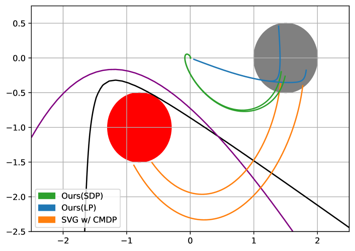
Figure 2. Trajectories under the learned controllers from our approach with SDP and LP, and from SVG (with shielding at testing) for the PJ example. Initial space $X_{0}$ is in grey, and unsafe region $X_{u}$ is in red. The barrier function 0-level plot by ours with the SDP formulation is in black and with the LP formulation is in purple.

Inverted Pendulum (Stability). We consider the inverted pendulum example from the gym environment (Brockman et al., 2016) by a non-linear controller with $\sin{\varphi}$ and $\cos{\varphi}$ terms. The pendulum can be expressed

$$\ddot{\varphi}=-\frac{g}{l}sin(\varphi)-\frac{d}{ml^{2}}\dot{\varphi}+\frac{u}{ml^{2}},$$

where $\varphi$ is the angle deviation. System state $(\varphi,\dot{\varphi})\in\{\varphi^{2}+\dot{\varphi}^{2}\leq 2\}$. $m=1,l=1,d=0.1$. Unknown parameter $g\in[9,10.5]$. $X_{0}=\{\varphi^{2}+\dot{\varphi}^{2}\leq 1\}$. For the $\sin$ function, we conduct variable transformation with $p=\sin(\varphi)$ and $q=\cos(\varphi)$, so that the dynamics can be transformed into a 4D polynomial system. Fig. 3 shows the trajectories from our approach (with SDP and LP) and from SVG, along with the Lyapunov function generated by our approach with SDP. The SVG fails to generate a Lyapunov function with polynomial degree up to 6 during the entire learning, as shown in Table 1 while our approach succeeds with quadratic certificates by both SDP and LP.

Figure 3. Trajectories on $(\varphi,\dot{\varphi})$ under the learned controllers from our approach by SDP and LP, and from baseline SVG for the Pendulum example. The right subplot shows the affiliated Lyapunov function obtained by SDP for the learned controller in our approach.

Lane Keeping (Safety and Stability). We consider a lane keeping example (Chen et al., 2014), where we try to derive a linear controller with barrier and Lyapunov certificate functions for both safety and stability. The system can be expressed as $\dot{x}=Ax+Bu$, where

$$A=\begin{bmatrix}0&1&v_{x}&0\\ 0&\frac{-(C_{\alpha f}+C_{\alpha r})}{mv_{x}}&0&\frac{bC_{\alpha r}-aC_{\alpha f}}{mv_{x}}-v_{x}+\alpha_{1}\\ 0&0&0&1\\ 0&\frac{bC_{\alpha r}-aC_{\alpha f}}{I_{z}v_{x}}&0&\frac{-(a^{2}C_{\alpha f}+b^{2}C_{\alpha r})}{I_{z}v_{x}}+\alpha_{2}\end{bmatrix},B=\begin{bmatrix}0\\ \frac{C_{\alpha f}}{m}\\ 0\\ \frac{aC_{\alpha f}}{I_{z}}\end{bmatrix}.$$

Here, $x=(y,v_{y},\psi_{e},r)^{T}$ is the system state with lateral displacement error $y$, lateral velocity $v_{y}$, yaw angle error $\psi_{e}$ and yaw rate $r$. Control input $u$ represents the steering angle at the front tire. $v_{x}$ is the longitudinal vehicle velocity. $\alpha_{1}\in[-15,5],\alpha_{2}\in[-10,-1]$ are the unknown parameters and other symbols are all known constants. $X_{0}=\{\|x-x_{0}\|_{2}\leq 0.2\}$, $X_{u}=\{\|x-x_{u}\|_{2}\leq 1\}$, and $X=\{\|x\|_{2}\leq 3\}$, where $x_{0}=(0.4,2,0.5,0)^{T}$ and $x_{u}=(2,2,0,1)^{T}$. Fig. 4 shows the simulated system trajectories under the controllers from our approach with SDP and LP, and from the SVG with CMDP. It also shows the barrier function value and the Lyapunov function value generated by our approach with LP, along with the trajectories over time. The SVG with CMDP can generate a quadratic Lyapunov function for stability but fails to find a barrier function for safety, as also shown in Table 1. LP succeeds with polynomial degree $6$ for barrier function and SDP succeeds with degree $4$. Therefore, SDP takes shorter time for each iteration in this example.

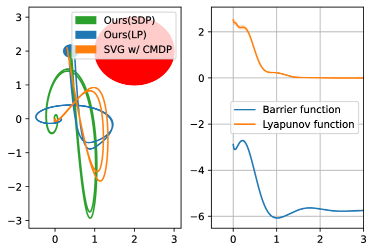
Figure 4. Left: Trajectories on $(y,v_{y})$ under the learned controllers from ours and from SVG with CMDP for Lane Keeping example. Right: Barrier and Lyapunov function values generated by our approach with LP, along with trajectories.

Attitude Control(Stability). The attitude control example (Huang et al., 2022) is the most complex one we tested. It has 6D state and 3D control input, which can be expressed as

$$\dot{\omega}_{1}=\alpha_{1}({u_{0}}+{\omega_{2}\omega_{3}}),$$

$$\dot{\omega}_{2}=\alpha_{2}({u_{1}}-{3\omega_{1}\omega_{3}}),$$

$$\dot{\omega}_{3}=u_{2}+2\omega_{1}\omega_{2},$$

$$\dot{\psi}_{1}{=}0.5\left(\omega_{2}(\psi_{1}\psi_{2}{-}{\psi_{3}}){+}\omega_{3}(\psi_{1}\psi_{3}{+}{\psi_{2}}){+}\omega_{1}({\psi_{1}^{2}}{+}{1})\right),$$

$$\dot{\psi}_{2}{=}0.5\left(\omega_{1}(\psi_{1}\psi_{2}{+}{\psi_{3}}){+}\omega_{3}(\psi_{2}\psi_{3}{-}\psi_{1}){+}\omega_{2}({\psi_{1}^{2}}{+}{1})\right),$$

$$\dot{\psi}_{3}{=}0.5\left(\omega_{1}(\psi_{1}\psi_{3}{-}\psi_{2}){+}\omega_{2}(\psi_{2}\psi_{3}{+}\psi_{1}){+}\omega_{3}({\psi_{3}^{2}}{+}{1})\right),$$

where the state $x=(\omega,\psi)$ consists of the angular velocity vector in a body-fixed frame $\omega\in\mathbb{R}^{3}$ and the Rodrigues parameter vector $\psi\in\mathbb{R}^{3}$. $u\in\mathbb{R}^{3}$ is the control torque. State space $X=\{x\ |\ ||x||_{2}\leq 2\}$, unknown dynamical parameters $\alpha_{1}\in[-1,2],\alpha_{2}\in[-0.5,1.5]$.

Our approach can successfully find a cubic polynomial controller with a quadratic Lyapunov function for stability with both SDP and LP, while SVG cannot generate a Lyapunov function for the entire learning process. Fig. 5 shows the simulated trajectories by learned controllers from different approaches.

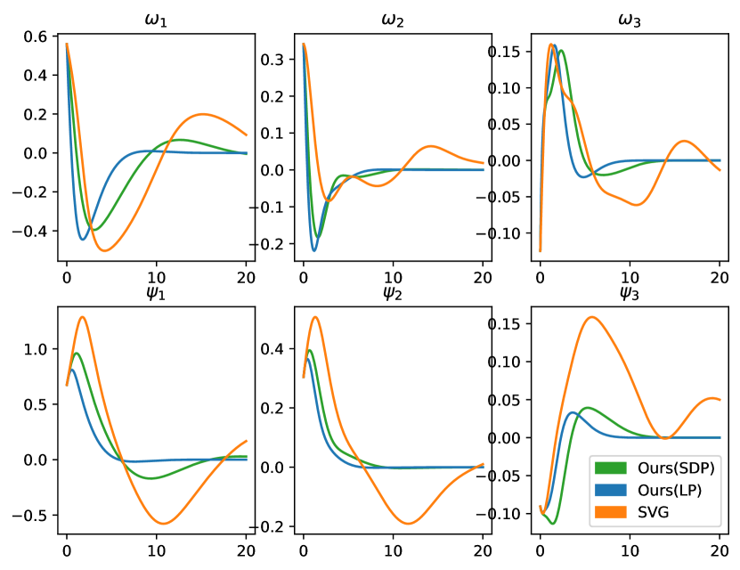
Figure 5. Trajectory on each dimension under the learned controllers from SVG and our approach for Attitude Control.

Timing Complexity of SDP and LP Relaxation: We first test the timing efficiency of SDP and LP in each iteration for the examples introduced before, with the polynomial degrees for certificates set as in Table 1, and the timing results are summarized in Table 2. LP does not show a big advantage, but note that most certificate functions are quadratic in Table 1.

Thus, to further test the scalability of SDP and LP for higher-dimensional systems, we raise the degree of certificates from 2 up to 6 in testing, with runtime shown in Fig. 6. We also show that the total number of variables of LP is fewer than SDP’s in the Attitude Control example in Table 3, especially for higher-dimensional systems. These demonstrate LP’s advantage in scalability, and we plan to explore it further in future work for larger examples.

Table 2. Averaged running time of each iteration by SDP and LP in our approach, with the degree shown in Table 1. LP is typically a bit more efficient than SDP, except for generating barrier certificate in the Lane Keeping example, where SDP succeeds in polynomial degree $4$ while LP needs degree $6$.

	PJ	Pendulum	Lane Keep	Att. Control
SDP(s)	0.95(B)	1.03(L)	2.55(B), 0.45(L)	7.32(L)
LP(s)	0.58(B)	0.81(L)	14.8(B), 0.4(L)	6.52(L)

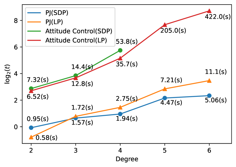
Figure 6. Averaged running time of each iteration by LP and SDP in PJ and Attitude Control examples under different degrees of certificate functions, shown in $\log_{2}$ magnitude with values on the plot. SDP reports timeout with degree 5 and 6 in Attitude Control, while LP can succeed. SDP is faster in the low-dimensional PJ example while LP has better scalability for the higher-dimensional systems.

Table 3. Number of variables in the Attitude Control example under different degree of certificate functions.

Degree	2	3	4	5	6
SDP	475	4042	4168	26078	26502
LP	302	664	1380	2675	4849

6. Conclusion

In this paper, we present a joint differentiable optimization and verification framework for certified reinforcement learning, by formulating and solving a novel bilevel optimization problem in an end-to-end differentiable manner, leveraging the gradients from both the certificates and the value function. Experimental results demonstrate the effectiveness of our approach in finding controllers with certificates for guaranteeing system safety and stability.

References

- (1)
- Agrawal et al. (2019) Akshay Agrawal, Brandon Amos, Shane Barratt, Stephen Boyd, Steven Diamond, and J Zico Kolter. 2019. Differentiable Convex Optimization Layers. Advances in Neural Information Processing Systems 32 (2019), 9562–9574.
- Barratt et al. (2021) Shane Barratt, Guillermo Angeris, and Stephen Boyd. 2021. Automatic repair of convex optimization problems. Optimization and Engineering 22, 1 (2021).
- Berkenkamp et al. (2017) Felix Berkenkamp, Matteo Turchetta, Angela Schoellig, and Andreas Krause. 2017. Safe model-based reinforcement learning with stability guarantees. Advances in neural information processing systems 30 (2017).
- Brockman et al. (2016) Greg Brockman, Vicki Cheung, Ludwig Pettersson, Jonas Schneider, John Schulman, Jie Tang, and Wojciech Zaremba. 2016. Openai gym. arXiv preprint arXiv:1606.01540 (2016).
- Chang et al. (2019) Ya-Chien Chang, Nima Roohi, and Sicun Gao. 2019. Neural lyapunov control. Advances in neural information processing systems 32 (2019).
- Chen et al. (2014) Bo-Chiuan Chen, Bi-Cheng Luan, and Kangwon Lee. 2014. Design of lane keeping system using adaptive model predictive control. In 2014 IEEE International Conference on Automation Science and Engineering (CASE). IEEE, 922–926.
- Chen et al. (2020) Shaoru Chen, Mahyar Fazlyab, Manfred Morari, George J Pappas, and Victor M Preciado. 2020. Learning lyapunov functions for piecewise affine systems with neural network controllers. arXiv preprint arXiv:2008.06546 (2020).
- Dawson et al. (2022a) Charles Dawson, Sicun Gao, and Chuchu Fan. 2022a. Safe Control with Learned Certificates: A Survey of Neural Lyapunov, Barrier, and Contraction methods. arXiv preprint arXiv:2202.11762 (2022).
- Dawson et al. (2022b) Charles Dawson, Zengyi Qin, Sicun Gao, and Chuchu Fan. 2022b. Safe nonlinear control using robust neural lyapunov-barrier functions. In Conference on Robot Learning. PMLR, 1724–1735.
- Fan et al. (2020) Jiameng Fan, Chao Huang, Xin Chen, Wenchao Li, and Qi Zhu. 2020. ReachNN*: A Tool for Reachability Analysis of Neural-Network Controlled Systems. In Automated Technology for Verification and Analysis, Dang Van Hung and Oleg Sokolsky (Eds.). Springer International Publishing, Cham, 537–542.
- Fu and Dasgupta (2000) Minyue Fu and Soura Dasgupta. 2000. Parametric Lyapunov functions for uncertain systems: The multiplier approach. In Advances in linear matrix inequality methods in control. SIAM, 95–108.
- Guo et al. (2020) Meichen Guo, Claudio De Persis, and Pietro Tesi. 2020. Learning control for polynomial systems using sum of squares relaxations. In CDC. IEEE, 2436–2441.
- Handelman (1988) David Handelman. 1988. Representing polynomials by positive linear functions on compact convex polyhedra. Pacific J. Math. 132, 1 (1988), 35–62.
- Heess et al. (2015) Nicolas Heess, Gregory Wayne, David Silver, Timothy Lillicrap, Tom Erez, and Yuval Tassa. 2015. Learning Continuous Control Policies by Stochastic Value Gradients. Advances in Neural Information Processing Systems 28 (2015).
- Huang et al. (2022) Chao Huang, Jiameng Fan, Xin Chen, Wenchao Li, and Qi Zhu. 2022. Polar: A polynomial arithmetic framework for verifying neural-network controlled systems. In ATVA. Springer, 414–430.
- Huang et al. (2019) Chao Huang, Jiameng Fan, Wenchao Li, Xin Chen, and Qi Zhu. 2019. ReachNN: Reachability analysis of neural-network controlled systems. ACM Transactions on Embedded Computing Systems (TECS) 18, 5s (2019), 1–22.
- Jin et al. (2021) Wanxin Jin, Shaoshuai Mou, and George J Pappas. 2021. Safe pontryagin differentiable programming. NeurIPS 34 (2021), 16034–16050.
- Jin et al. (2020) Wanxin Jin, Zhaoran Wang, Zhuoran Yang, and Shaoshuai Mou. 2020. Neural certificates for safe control policies. arXiv preprint arXiv:2006.08465 (2020).
- Khalil (2002) Hassan K Khalil. 2002. Nonlinear systems third edition. (2002).
- Knight (2002) John C Knight. 2002. Safety critical systems: challenges and directions. In Proceedings of the 24th international conference on software engineering. 547–550.
- Koch et al. (2019) William Koch, Renato Mancuso, Richard West, and Azer Bestavros. 2019. Reinforcement learning for UAV attitude control. TCPS 3, 2 (2019), 1–21.
- Kong et al. (2013) Hui Kong, Fei He, Xiaoyu Song, William NN Hung, and Ming Gu. 2013. Exponential-condition-based barrier certificate generation for safety verification of hybrid systems. In CAV. Springer, 242–257.
- Lasserre (2005) Jean B Lasserre. 2005. Polynomial programming: LP-relaxations also converge. SIAM Journal on Optimization 15, 2 (2005), 383–393.
- Lindemann et al. (2021) Lars Lindemann, Haimin Hu, Alexander Robey, Hanwen Zhang, Dimos Dimarogonas, Stephen Tu, and Nikolai Matni. 2021. Learning Hybrid Control Barrier Functions from Data. In Conference on Robot Learning. PMLR, 1351–1370.
- Liu et al. (2015) Jiang Liu, Naijun Zhan, Hengjun Zhao, and Liang Zou. 2015. Abstraction of elementary hybrid systems by variable transformation. In International Symposium on Formal Methods. Springer, 360–377.
- Liu et al. (2022) Xiangguo Liu, Chao Huang, Yixuan Wang, Bowen Zheng, and Qi Zhu. 2022. Physics-aware safety-assured design of hierarchical neural network based planner. In 2022 ACM/IEEE 13th International Conference on Cyber-Physical Systems (ICCPS). IEEE, 137–146.
- Liu et al. (2023) Xiangguo Liu, Ruochen Jiao, Bowen Zheng, Dave Liang, and Qi Zhu. 2023. Safety-driven Interactive Planning for Neural Network-based Lane Changing. In Proceedings of the 28th Asia and South Pacific Design Automation Conference. 39–45.
- Luo and Ma (2021) Yuping Luo and Tengyu Ma. 2021. Learning Barrier Certificates: Towards Safe Reinforcement Learning with Zero Training-time Violations. NeurIPS 34 (2021).
- Lyapunov (1992) Aleksandr Mikhailovich Lyapunov. 1992. The general problem of the stability of motion. International journal of control 55, 3 (1992), 531–534.
- Nie and Schweighofer (2007) Jiawang Nie and Markus Schweighofer. 2007. On the complexity of Putinar’s Positivstellensatz. Journal of Complexity 23, 1 (2007), 135–150.
- Nocedal and Wright (1999) Jorge Nocedal and Stephen J Wright. 1999. Numerical optimization. Springer.
- Papachristodoulou and Prajna (2002) Antonis Papachristodoulou and Stephen Prajna. 2002. On the construction of Lyapunov functions using the sum of squares decomposition. In CDC, Vol. 3. IEEE, 3482–3487.
- Prajna (2006) Stephen Prajna. 2006. Barrier certificates for nonlinear model validation. Automatica 42, 1 (2006), 117–126.
- Prajna and Jadbabaie (2004) Stephen Prajna and Ali Jadbabaie. 2004. Safety verification of hybrid systems using barrier certificates. In HSCC. Springer, 477–492.
- Prajna et al. (2002) Stephen Prajna, Antonis Papachristodoulou, and Pablo A Parrilo. 2002. Introducing SOSTOOLS: A general purpose sum of squares programming solver. In Proceedings of the 41st CDC, 2002., Vol. 1. IEEE, 741–746.
- Qin et al. (2021) Zengyi Qin, Kaiqing Zhang, Yuxiao Chen, Jingkai Chen, and Chuchu Fan. 2021. Learning Safe Multi-Agent Control with Decentralized Neural Barrier Certificates. arXiv preprint arXiv:2101.05436 (2021).
- Robey et al. (2020) Alexander Robey, Haimin Hu, Lars Lindemann, Hanwen Zhang, Dimos V Dimarogonas, Stephen Tu, and Nikolai Matni. 2020. Learning control barrier functions from expert demonstrations. In CDC. IEEE, 3717–3724.
- Robey et al. (2021) Alexander Robey, Lars Lindemann, Stephen Tu, and Nikolai Matni. 2021. Learning robust hybrid control barrier functions for uncertain systems. IFAC-PapersOnLine 54, 5 (2021), 1–6.
- Sankaranarayanan et al. (2013) Sriram Sankaranarayanan, Xin Chen, et al. 2013. Lyapunov Function Synthesis using Handelman Representations. IFAC Proceedings Volumes 46, 23 (2013).
- Srinivasan et al. (2020) Krishnan Srinivasan, Benjamin Eysenbach, Sehoon Ha, Jie Tan, and Chelsea Finn. 2020. Learning to be safe: Deep rl with a safety critic. arXiv preprint arXiv:2010.14603 (2020).
- Stooke et al. (2020) Adam Stooke, Joshua Achiam, and Pieter Abbeel. 2020. Responsive safety in reinforcement learning by pid lagrangian methods. In ICML. PMLR, 9133–9143.
- Sutton and Barto (2018) Richard S Sutton and Andrew G Barto. 2018. Reinforcement learning: An introduction. MIT press.
- Thananjeyan et al. (2021) Brijen Thananjeyan, Ashwin Balakrishna, Suraj Nair, Michael Luo, Krishnan Srinivasan, Minho Hwang, Joseph E Gonzalez, Julian Ibarz, Chelsea Finn, and Ken Goldberg. 2021. Recovery rl: Safe reinforcement learning with learned recovery zones. IEEE Robotics and Automation Letters 6, 3 (2021), 4915–4922.
- Tsukamoto and Chung (2020) Hiroyasu Tsukamoto and Soon-Jo Chung. 2020. Neural contraction metrics for robust estimation and control: A convex optimization approach. IEEE Control Systems Letters 5, 1 (2020), 211–216.
- Wang et al. (2022b) Yixuan Wang, Chao Huang, Zhaoran Wang, Zhilu Wang, and Qi Zhu. 2022b. Design-while-verify: correct-by-construction control learning with verification in the loop. In Proceedings of the 59th Design Automation Conference. 925–930.
- Wang et al. (2021) Yixuan Wang, Chao Huang, Zhilu Wang, Shichao Xu, Zhaoran Wang, and Qi Zhu. 2021. Cocktail: Learn a better neural network controller from multiple experts via adaptive mixing and robust distillation. In 2021 58th ACM/IEEE Design Automation Conference (DAC). IEEE, 397–402.
- Wang et al. (2020) Yixuan Wang, Chao Huang, and Qi Zhu. 2020. Energy-efficient control adaptation with safety guarantees for learning-enabled cyber-physical systems. In 2020 International Conference On Computer Aided Design (ICCAD). IEEE, 1–9.
- Wang et al. (2022c) Yixuan Wang, Simon Sinong Zhan, Ruochen Jiao, Zhilu Wang, Wanxin Jin, Zhuoran Yang, Zhaoran Wang, Chao Huang, and Qi Zhu. 2022c. Enforcing Hard Constraints with Soft Barriers: Safe Reinforcement Learning in Unknown Stochastic Environments. arXiv preprint arXiv:2209.15090 (2022).
- Wang et al. (2022a) Zhilu Wang, Chao Huang, and Qi Zhu. 2022a. Efficient Global Robustness Certification of Neural Networks via Interleaving Twin-Network Encoding. In DATE’22: Proceedings of the Conference on Design, Automation and Test in Europe.
- Wei et al. (2017) T. Wei, Yanzhi Wang, and Q. Zhu. 2017. Deep reinforcement learning for building HVAC control. In 2017 54th ACM/EDAC/IEEE Design Automation Conference (DAC). 1–6. https://doi.org/10.1145/3061639.3062224
- Wolfe (1969) Philip Wolfe. 1969. Convergence conditions for ascent methods. SIAM review 11, 2 (1969), 226–235.
- Xu et al. (2020) Shichao Xu, Yixuan Wang, Yanzhi Wang, Zheng O’Neill, and Qi Zhu. 2020. One for many: Transfer learning for building hvac control. In Proceedings of the 7th ACM international conference on systems for energy-efficient buildings, cities, and transportation. 230–239.
- Zhao et al. (2020) Hengjun Zhao, Xia Zeng, Taolue Chen, and Zhiming Liu. 2020. Synthesizing barrier certificates using neural networks. In HSCC. 1–11.
- Zhu et al. (2021) Qi Zhu, Chao Huang, Ruochen Jiao, Shuyue Lan, Hengyi Liang, Xiangguo Liu, Yixuan Wang, Zhilu Wang, and Shichao Xu. 2021. Safety-assured design and adaptation of learning-enabled autonomous systems. In Proceedings of the 26th Asia and South Pacific Design Automation Conference. 753–760.
- Zhu et al. (2020) Qi Zhu, Wenchao Li, Hyoseung Kim, Yecheng Xiang, Kacper Wardega, Zhilu Wang, Yixuan Wang, Hengyi Liang, Chao Huang, Jiameng Fan, and Hyunjong Choi. 2020. Know the Unknowns: Addressing Disturbances and Uncertainties in Autonomous Systems. In Proceedings of the 39th International Conference on Computer-Aided Design (Virtual Event, USA) (ICCAD ’20).
- Zhu and Sangiovanni-Vincentelli (2018) Qi Zhu and Alberto Sangiovanni-Vincentelli. 2018. Codesign Methodologies and Tools for Cyber–Physical Systems. Proc. IEEE 106, 9 (Sep. 2018), 1484–1500. https://doi.org/10.1109/JPROC.2018.2864271