Simulating surface height and terminus position for marine outlet glaciers using a level set method with data assimilation

Abstract

We implement a data assimilation framework for integrating ice surface and terminus position observations into a numerical ice-flow model. The model uses the well-known shallow shelf approximation (SSA) coupled to a level set method to capture ice motion and changes in the glacier geometry. The level set method explicitly tracks the evolving ice–atmosphere and ice–ocean boundaries for a marine outlet glacier. We use an Ensemble Transform Kalman Filter to assimilate observations of ice surface elevation and lateral ice extent by updating the level set function that describes the ice interface. Numerical experiments on an idealized marine-terminating glacier demonstrate the effectiveness of our data assimilation approach for tracking seasonal and multi-year glacier advance and retreat cycles. The model is also applied to simulate Helheim Glacier, a major tidewater-terminating glacier of the Greenland Ice Sheet that has experienced a recent history of rapid retreat. By assimilating observations from remotely-sensed surface elevation profiles we are able to more accurately track the migrating glacier terminus and glacier surface changes. These results support the use of data assimilation methodologies for obtaining more accurate predictions of short-term ice sheet dynamics.

1 Introduction

The rapid increases in ice loss from the Earth’s cryosphere over the past few decades [53] and ongoing uncertainty regarding the future of the ice sheets [7, 47] highlight the urgent need to integrate any available in-situ and remotely-sensed observations along with state-of-the-art numerical models [28] in order to better understand current and future changes. For instance, ice dynamical imbalances have been a significant source of ice loss with increased discharge from outlet glaciers in both Antarctica [40] and the Greenland Ice Sheet [22]. Tidewater outlet glaciers are highly sensitive to changes occurring at their terminus [7, 27], with potentially dramatic consequences [12, 51, 58] that make it challenging to confidently predict the rate of future mass loss. Because of these dynamic instabilities, considerable uncertainty remains when projecting dynamic ice behaviour into the future. Predicting short-term (inter- and intra-annual, multi-year) ice dynamics could be improved with the seamless integration of time-ordered observations into dynamical ice sheet models. In this paper, we develop a data assimilation approach combined with a level set method to estimate the ice surface and terminus position over seasonal and multi-year time scales.

Data assimilation combines observational data with a dynamical system model to compute accurate estimates of the current and future states of the system together with a measure of the uncertainty in those states [30]. Data assimilation can be helpful in reducing uncertainties in model state and parameters [46]. Historically, data assimilation has been used in operational meteorology and oceanography [26], while more recently it has been applied to subjects as diverse as seismology [19], nuclear fusion [39], medicine [10] and agronomy [24]. Glaciologists have also begun exploiting data assimilation techniques to incorporate time-ordered observations into their modelling studies [3, 4, 16], and with the recent growth in availability of observations [8, 15, 31, 56] it is only natural that data assimilation will increase in importance in the glaciology community.

Due to the paucity of observations measuring glacier bed properties ice sheet modellers have long employed static inverse techniques to determine basal conditions from surface velocity observations [18, 34, 49]. These methods have also been used for estimating other unknowns, such as optimal initial conditions from available observations [48]. More recently, time-dependent adjoints have been considered for state and parameter estimation as well as sensitivity analysis [9, 17]. In this paper, we utilize a sequential data assimilation method based on the ensemble Kalman filter (EnKF), which is a Monte Carlo approach to the Bayesian update problem. Such methods have also been applied in glaciology. For example, Bonan et al. [4] developed an Ensemble Transform Kalman Filter (ETKF) [2, 23] for a Shallow Ice Approximation (SIA) model of ice dynamics in order to estimate jointly the bedrock topography, ice thickness and basal sliding parameter for an ice sheet. Bonan et al. [3] further investigated such data assimilation approaches to estimate the state of a grounded ice sheet simulated using a moving mesh method. Gillet-Chaulet [16] has recently published a study of the EnKF method to initialize a marine ice sheet model including grounding line migration. There is immense potential to further exploit these sequential data assimilation techniques in forecast models of marine ice sheets, tidewater glaciers and rapidly retreating outlet glaciers.

The level set method (LSM) is a versatile numerical technique for simulating the motion of dynamically evolving surfaces and has found many applications in image processing [44], fire front propagation [36, 52], tumor growth [35, 38], materials science [41], computational fluid dynamics [52], among others. The LSM was first employed to track ice surfaces by Pralong and Funk [50], who simulated the steady-state configuration of a glacier by computing the stationary form of the level set equation. Pralong and Funk [50] compared different numerical solutions of the model with other published analytical and numerical solutions. Bondzio et al. [5] have also developed a LSM-based 2D plan-view model to study the dynamic evolution of a glacier calving front, but they did not consider the elevation of the ice sheet. Recently, we have developed a level set algorithm for explicitly tracking ice interfaces, moving ice margin, and grounding line position in the context of a fixed grid finite-difference scheme [20], which challenges the assertion in [57] that fixed grid methods are inadequate for capturing grounding line or terminus position.

There have been some recent attempts at implementing data assimilation for applications using the level set method. One example is front tracking for oil spills, for which Li et al. [32] proposed a level set based image assimilation method that captures the complex topological structure of oil slicks and polluted regions to minimize any delays in cleanup efforts because of inaccurate predictions from observations. A second example relates to wildfire spread, where Mandel et al. [37] used an EnKF method to estimate the state of a wildland fire using available data and a model which accounts for interactions between the fire and the atmosphere. These authors implemented a level set method coupled with an atmospheric model to deliver short-term predictions of fire propagation in a timely and expedient manner.

We develop a glacier model that estimates ice surface elevation and terminus position by combining the level set approach developed by Hossain et al. [20] with the advantages of data assimilation when observations are available to reinitialize the model. We begin in Section 2 by introducing our ice sheet model, which is a shallow shelf approximation (SSA) [6] that is closely related to the SIA model. Section 3 describes the details of the level set method used to capture the evolving ice sheet boundary. In Section 4 we apply the Ensemble Transform Kalman Filter (ETKF) to our state estimation problem, and in Section 5 we outline our hybrid SSA–LSM–ETKF algorithm that combines the various algorithm components. In Section 6 we demonstrate the effectiveness of the SSA–LSM–ETKF method for simulating an idealized ice sheet test problem, as well as a more realistic problem using actual data taken from Helheim Glacier, Greenland.

2 Ice flow equations

In this section, we introduce the ice sheet model corresponding to the shallow shelf approximation (SSA) for ice streams. We also describe our numerical approach for computing the SSA velocities, which are used as input to the LSM algorithm for evolving the ice sheet and tracking the ice–air and ice–water interfaces (described later in Section 3). The ETKF algorithm is then used to update the ice surface and terminus positions using observations (see Section 4).

The flow of an ice sheet is a large-scale fluid dynamics problem that has many features in common with other geophysical systems such as atmospheric or ocean circulation. As such we describe the ice motion using a velocity field $\bm{\mathrm{u}}(x,y,z,t)$ that is governed by the Navier-Stokes equations:

$$\frac{\partial\rho}{\partial t}+\nabla\cdot(\rho\bm{\mathrm{u}}) =0,$$ (1)

$$\rho(\bm{\mathrm{u}}_{t}+\bm{\mathrm{u}}\cdot\nabla\bm{\mathrm{u}}) =-\nabla p+\nabla\cdot\tau_{i,j}+\rho\bm{\mathrm{g}},$$ (2)

where $\rho$ is the ice density, $p$ is pressure, $\tau_{i,j}$ is the deviatoric stress tensor, and $\bm{\mathrm{g}}=(0,0,-g)$ is the acceleration due to gravity. The uppermost compressible layer of an ice sheet is shallow compared to the entire body of ice [11], and consists of snow and firn (compacted snow that is transforming into glacier ice). Moreover, there is little variation in ice density due to changes in depth or temperature, so that the ice can be considered an incompressible fluid for which the mass conservation equation (1) simplifies to $\nabla\cdot\bm{\mathrm{u}}=0$.

2.1 Stokes approximation

Within glaciers, the ice behaves as a very slow-moving fluid so that inertial forces can be neglected and thus

$$\rho(\bm{\mathrm{u}}_{t}+\bm{\mathrm{u}}\cdot\nabla\bm{\mathrm{u}})\approx 0,$$

which when substituted into (2) yields the linearized Stokes approximation. Furthermore, ice flow models typically use a strain-rate-dependent viscosity to describe ice rheology, for which the most widely used form (called Glen’s flow law) is derived by fitting empirical measurements of ice deformation to a power law [11]. The standard model for isothermal ice flow is therefore given by an augmented version of the Stokes equations:

(incompressibility) $$\nabla\cdot\bm{\mathrm{u}} =0,$$ (3)

(Stokes equations, stress balance) $$0 =-\nabla p+\nabla\cdot\tau_{i,j}+\rho\bm{\mathrm{g}},$$ (4)

(Glen’s flow law) $$\mathcal{D}u_{i,j} =A\tau^{\alpha-1}\tau_{i,j},$$ (5)

where the strain rate tensor is $\mathcal{D}u_{i,j}=\frac{1}{2}\left(\frac{\partial u_{i}}{\partial x_{j}}+\frac{\partial u_{j}}{\partial x_{i}}\right)$ and $\tau^{2}=\frac{1}{2}\tau_{i,j}\tau_{j,i}$ (with the summation convention assumed for repeated indices). A typical value of the exponent in Glen’s flow law is $\alpha=3$. Because the Stokes equations contain no time derivative, the ice velocity $\bm{\mathrm{u}}$, pressure $p$, and stress field $\tau_{i,j}$ are determined simultaneously from the gravitational force $\rho\bm{\mathrm{g}}$, ice softness $A$, and boundary stresses.

2.2 Shallow shelf approximation (SSA)

The Stokes equations (3)–(5) remain challenging to implement on a routine basis. The SSA is a well-established and frequently used approximation that neglects vertical shear [33], which is valid for ice shelves and ice streams because they are characterized by low basal drag. We introduce the SSA here for a two-dimensional grounded shallow marine ice sheet as pictured in Fig. 1. Let $x$ denote the horizontal coordinate in the flow direction with $x=0$ defining the up-glacier boundary of the ice stream, and let $z$ be the vertical coordinate measured upward from sea level. In the horizontal direction, the ice sheet extends from $x=0$ to the location $x=x_{\mathrm{g}}$ that separates grounded ice from the surrounding ocean, which is known as the grounding line (and terminus position, if a floating ice shelf is absent). We then define $H(x,t)$ as the ice thickness at position $x$ and time $t$, and $b(x)$ as the bedrock surface height, so that the location of the upper ice surface in contact with the atmosphere is at $z=h(x,t)=H(x,t)+b(x)$ (see Fig. 1).

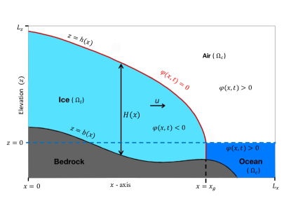
Fig. 1: A grounded, marine-terminated ice sheet profile, illustrating how the level set function $\varphi(\bm{\mathrm{x}},t)$ separates the domain into three regions: the ice region ($\Omega_{i}$ with $\varphi<0$), the air/ocean region lying outside the ice ($\Omega_{c}$ with $\varphi>0$), and the interface between them ($z=h=H+b$ along $\varphi=0$).

The SSA model for a grounded ice sheet occupying the region $0<x<x_{\mathrm{g}}(t)$ is a nonlinear differential equation

$$\left(2A^{-1/\alpha}H|u_{x}|^{1/\alpha-1}u_{x}\right)_{x}-C|u|^{\beta-1}u=\rho gHh_{x},$$ (6)

where we note that the spatial domain is time-dependent owing to changes in the terminus position $x_{\mathrm{g}}(t)$. This is a statement of momentum conservation that is obtained from Eqs. (3)–(5). The first term in Eq. (6) is the vertically-integrated longitudinal stress. The second term $\tau_{\mathrm{b}}=C|u|^{\beta-1}u$ represents the basal shear stress, where $C$ is a friction coefficient (with $C\equiv 0$ for an ice shelf) and the friction exponent $\beta$ has a typical value of $\beta=\frac{1}{3}$. The final term on the right hand side is the driving stress due to gravity, $\tau_{\mathrm{d}}=\rho gHh_{x}$. As a result, the SSA equation represents a stress balance wherein longitudinal strain rates are determined by the integrated ice hardness (through the coefficient $2A^{-1/\alpha}H$), the slipperiness of the bedrock (friction coefficient $C$ and exponent $\beta$), and the geometry of the ice sheet (thickness $H$ and surface slope $h_{x}$).

Because Eq. (6) is a 1D nonlinear second-order equation for $u$, two boundary conditions are required. We also note that effects of time variation only appear implicitly through changes in the ice thickness $H(x,t)$. For this reason, we will often write the ice velocity $u(x,t)$ as $u(x)$, treating the time $t$ as a parameter. On the left-hand boundary or the up-glacier boundary, the ice is simply assumed to have a constant velocity:

$$u=u_{\mathrm{in}}\quad\textrm{at}\quad x=0.$$ (7)

At the terminus position, the right-most point where ice begins to float, we impose the flotation condition

$$h=(1-\rho/\rho_{\mathrm{w}})H\quad\textrm{at}\quad x=x_{\mathrm{g}}.$$

Upon substituting this expression into (6) and neglecting basal friction for floating ice (by dropping the term $C|u|^{\beta-1}u$), we obtain the corresponding right hand boundary condition for $u$

$$2A^{-1/\alpha}H|u_{x}|^{1/\alpha-1}u_{x}=\frac{1}{2}\rho(1-\rho/\rho_{\mathrm{w}})gH^{2}\quad\textrm{at}\quad x=x_{\mathrm{g}}.$$ (8)

The SSA model only determines the horizontal ice velocity $u(x,t)$, but any ice sheet travelling over a non-uniform bedrock layer will also induce a vertical ice motion. We can easily obtain this vertical velocity of the ice stream by assuming that the bedrock is rigid and that no melting occurs at the bottom surface. In that case, we can impose a kinematic boundary condition that the ice velocity directed perpendicular to the rigid bedrock must vanish on the boundary itself ($\frac{\partial b}{\partial t}=0$). When combined with the incompressibility condition (3), this yields the vertical velocity corresponding to any horizontal velocity field $u$ as

$$w(x,z,t)=u(x,t)b_{x}-(z-b(x))u_{x}\quad\textrm{for}\quad 0\leqslant x\leqslant x_{\mathrm{g}},$$ (9)

where the 2D SSA velocity is $\bm{\mathrm{u}}(x,z,t)=\Big{(}u(x,t),\,w(x,z,t)\Big{)}$.

2.3 Numerical solution of the SSA

Taking the ice thickness as a given function $H(x)$, our aim is to solve the nonlinear differential equation (6) for the unknown velocity $u(x)$. We choose a spatial grid with constant spacing $\Delta x$ and $N_{x}$ equally-spaced points $x_{i}=i\Delta x$, and define corresponding solution approximations as $u_{i}\approx u(x_{i})$, where $N_{x}\Delta x\leqslant x_{\mathrm{g}}<(N_{x}+1)\Delta x$. Note that the SSA is a quasi-steady 1D approximation used to determine the velocity components $(u,w)$ in the $x$ and $z$ directions at any time $t$ based on the current height profile $H(x)$. At discrete times labelled $t^{k}$, velocity components are denoted by $u^{k}$, $w^{k}$, and ice thickness and surface height by $H^{k}$, $h^{k}$. For simplicity of notation, we will often suppress the superscript $k$ in the SSA algorithm.

The discrete equations for $u_{i}$ are solved using a Picard iteration approach that linearizes the nonlinear system. Letting $u^{(r)}$ denote the current velocity iterate, the Picard approach linearizes the equation by labeling various terms in the left hand side of (6) as follows:

$$\left(W^{(r-1)}u^{(r)}_{x}\right)_{x}-C\left|u^{(r-1)}\right|^{\beta-1}u^{(r)}=\rho gHh_{x},$$ (10)

where $W^{(r-1)}=2A^{-1/\alpha}H\left|u^{(r-1)}_{x}\right|^{1/\alpha-1}$, and noting that $\rho gHh_{x}$ remains constant for all iterations. For stability and accuracy reasons, the coefficient function $W^{(r)}$ is discretized with a compact, centered difference approximation so that the discrete form of the first term in (10) is

$$\left(W^{(r-1)}u^{(r)}_{x}\right)_{x}=\frac{W_{i+1/2}^{(r-1)}(u_{i+1}^{(r)}-u_{i}^{(r)})-W_{i-1/2}^{(r-1)}(u_{i}^{(r)}-u_{i-1}^{(r)})}{\Delta x^{2}}$$

where $W_{i+1/2}^{(r-1)}=2A^{-1/\alpha}\left(\frac{H_{i+1}+H_{i}}{2}\right)\left|\frac{u_{i+1}^{(r-1)}-u_{i}^{(r-1)}}{\Delta x}\right|^{1/\alpha-1}$. The corresponding discrete form of (10) is a linear system for $u_{i}^{(r)}$ that is solved in each iteration. In practice, we use a convergence tolerance of $10^{-10}$ in the max-norm which requires between 5 and 20 Picard iterations.

To obtain the initial velocity iterate $u^{(0)}$, we assume that the grounded ice ($0<x<x_{\mathrm{g}}$) is held in place by basal resistance only. Therefore, $u^{(0)}(x)=\left(-C^{-1}\rho gHh_{x}\right)^{1/\beta}$ and the boundary condition from (7) is imposed on the left. The right end condition (8) can be written as

$$u_{x}(x_{\mathrm{g}})=\frac{u_{N_{x}+1}-u_{N_{x}}}{\Delta x}=A\left(\frac{1}{4}\rho(1-\rho/\rho_{\mathrm{w}})gH(x_{\mathrm{g}})\right)^{\alpha}\,\,\mathrm{where}\,\,N_{x}\Delta x\leqslant x_{\mathrm{g}}<(N_{x}+1)\Delta x.$$ (11)

The discretized form of (10) at $x=x_{N_{x}}$ contains the value $u_{N_{x}+1}$, which is replaced using the relation (11) and then the “ghost” value $W_{N_{x}+1/2}$ can be determined using cubic extrapolation.

The vertical velocity is discretized using centered difference approximations for $b_{x}$ and $u_{x}$ to give

$$w_{i,j}=u_{i}\frac{b_{i+1}-b_{i-1}}{2\Delta x}-(z_{j}-b_{i})\frac{u_{i+1}-u_{i-1}}{2\Delta x},$$

with the boundary points handled using one-sided differences. Here, the vertical coordinate is discretized at points $z_{j}=j\Delta z$ with $j=0,1,\dots,N_{z}$ with $N_{z}=100$ points in practice. Because care has been taken to employ second-order difference approximations for all spatial derivatives, the SSA algorithm can be expected to converge with second-order accuracy in space, which has been confirmed in previous work [20].

Parameter	Symbol	Value	Units
Ice density	$\rho$	900	$\mathrm{kg/m^{3}}$
Water density	$\rho_{\mathrm{w}}$	1000	$\mathrm{kg/m^{3}}$
Ice softness	$A$	$5.6\times 10^{-17}$	$\mathrm{1/(Pa^{3}\,yr)}$
Gravitational acceleration	$g$	9.8	$\mathrm{m/s^{2}}$
Glen’s law exponent	$\alpha$	3	–
Friction exponent	$\beta$	1/3	–
Friction coefficient	$C$	[0.01, 0.015]   0.03	$\mathrm{MPa\,(yr/m)^{1/3}}$
Velocity at up-glacier boundary	$u_{\mathrm{in}}$	8.0   4.5	$\mathrm{km/yr}$
Front stress perturbation coefficient	$C_{F}$	1.0   [1.5, 3.5]	–
Domain length	$L_{x}$	10   40	$\mathrm{km}$
Domain height	$L_{z}$	400   1000	$\mathrm{m}$
Vertical grid dimension	$N_{z}$	100	–
Number of ensembles	$N_{e}$	50	–

Table 1: Values of the physical and numerical parameters. In the “value” column, when two numbers are separated by a “   ”, the first number corresponds to Experiments 1 and 2, and the second to Experiment 3.

3 Level set method

When the effect of vertical ice accumulation is incorporated into the ice velocity obtained from the 1D SSA model, the combined ice–air and ice–water interface evolves in two dimensions. In this section, we describe a numerical approach called the level set method (LSM) that is capable of accurately and efficiently tracking this ice interface in 2D. We provide only the essential details of the coupled SSA–LSM approach and direct the interested reader to Hossain et al. [20] for complete details, including computational studies based on an extensive suite of test cases.

The level set method was originally developed by Osher and Sethian [45] for capturing an evolving interface $\Gamma(t)$ implicitly in terms of a level set function $\varphi(\bm{\mathrm{x}},t)$. The function $\varphi$ is real-valued and differentiable on a space-time domain $\Omega\times\mathbb{R}_{+}$, where the spatial variable is $\bm{\mathrm{x}}\in\Omega$. The interface $\Gamma(t)\subset\Omega$ is a curve that evolves in time $t$ and is represented as the zero isosurface or level set ${\varphi(\bm{\mathrm{x}},t)=0}$, which propagates at a speed directed normal to the interface.

When tracking the interface in our ice sheet model, we employ a common approach in which the level set function is defined as a signed distance function

$$\varphi(\bm{\mathrm{x}},t)=\left\{\begin{array}[]{cl}-d(\bm{\mathrm{x}},\Gamma),&\mathrm{for}\,\,\bm{\mathrm{x}}\in\Omega_{i},\\ \phantom{-}d(\bm{\mathrm{x}},\Gamma),&\mathrm{for}\,\,\bm{\mathrm{x}}\in\Omega_{c},\\ 0,&\mathrm{for}\,\,\bm{\mathrm{x}}\in\Gamma,\end{array}\right.$$ (15)

where $\Omega_{i}$ represents the region inside the ice body, $\Omega_{c}$ is the region outside the ice (consisting of either air or water), $\Gamma$ is the ice–air or ice–water interface, and $\Omega=\Omega_{i}\cup\Omega_{c}\cup\Gamma$ (see Fig. 1). The value of the level set function corresponds to the Euclidean distance ${d(\bm{\mathrm{x}},\Gamma)}$ between any spatial location $\bm{\mathrm{x}}$ and the corresponding closest point on the interface $\Gamma$, with the sign chosen to be negative at points inside the ice region and positive outside.

3.1 Level set evolution

In order to derive an equation for the evolution of the level set function, we first require that any point $\bm{\mathrm{x}}(t)\in\Gamma(t)$ on the interface being tracked must satisfy $\varphi(\bm{\mathrm{x}}(t),t)=0$, which can be differentiated in time to obtain

$$\frac{\partial\varphi}{\partial t}+\nabla\varphi(\bm{\mathrm{x}}(t),t)\cdot\bm{\mathrm{x}}^{\prime}(t)=0.$$

Let $S$ represent the speed of the interface in the outward-pointing normal direction. Then

$$\bm{\mathrm{x}}^{\prime}(t)\cdot\bm{\mathrm{n}}=S\quad\textrm{where}\quad\bm{\mathrm{n}}=\nabla\varphi/\|\nabla\varphi\|,$$

and the evolution equation for the level set function may be re-written in the form of a Hamilton-Jacobi equation

$$\frac{\partial\varphi}{\partial t}+S\|\nabla\varphi\|=0.$$ (16)

The essential remaining component of the LSM is an expression for the normal speed $S$, which must incorporate the ice velocity field $\bm{\mathrm{u}}(\bm{\mathrm{x}},t)$ together with any accumulation or melting along $\Gamma$ [50]. Let $\omega(\bm{\mathrm{x}},t)$ denote the net accumulation rate of ice at the upper surface, which is a combination of snow accumulation and melting (or ablation) that can either be modelled separately or specified using observational data. If we assume that snowfall and melting correspond to vertical variations only, then the total ice velocity may be written as $\bm{\mathrm{u}}(\bm{\mathrm{x}},t)+\omega(\bm{\mathrm{x}},t)\bm{\mathrm{\hat{z}}}$ where $\bm{\mathrm{\hat{z}}}$ is the unit vector in the vertical direction. However, this velocity field is defined only inside the ice region $\Omega_{i}$, and because the level set equation is solved throughout the entire computational domain $\Omega$ we must also determine values of the so-called extended speed $S^{\mathrm{ext}}$ at points in $\Omega_{c}$ lying outside the ice region (see Fig. 2). Therefore, we can write the normal speed function as

$$S(\bm{\mathrm{x}},t)=\left\{\begin{array}[]{ll}\Big{(}\bm{\mathrm{u}}(\bm{\mathrm{x}},t)+\omega(\bm{\mathrm{x}},t)\bm{\mathrm{\hat{z}}}\Big{)}\cdot\bm{\mathrm{n}},&\mathrm{for}\,\,\bm{\mathrm{x}}\in\Omega_{i}\cup\Gamma,\\ S^{\mathrm{ext}},&\mathrm{for}\,\,\bm{\mathrm{x}}\in\Omega_{c}.\end{array}\right.$$ (19)

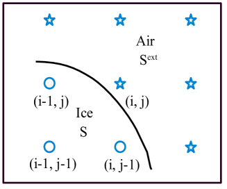
Fig. 2: The ice–air interface or zero level set of $\varphi$ is represented by a solid line, lying in the neighbourhood of a discrete point at location $(i,j)$. The interface speed $S$ is known at all points inside the ice, denoted by ‘$\circ$’ and the speed is extended outside the ice region to obtain $S^{\mathrm{ext}}$ at points ‘✩’.

We now complete the LSM algorithm description by illustrating how the extended velocity field is computed, which is based on the desirable assumption that $S^{\mathrm{ext}}$ should propagate level sets in such a way that the signed distance function is preserved. Following [59], $\varphi(\bm{\mathrm{x}}(t),t)$ remains a signed distance function if and only if

$$\nabla S^{\mathrm{ext}}\cdot\nabla\varphi=0.$$ (20)

Recognizing that interfaces evolving according to (16) may undergo topological changes, there are a large number of possible cases that must be considered relating to the configuration of the interface in the neighbourhood of any discrete point [52]. We illustrate how to implement (20) for the special case pictured in Fig. 2, where the point $(i,j)$ lies outside the ice region and $S^{\mathrm{ext}}$ is determined there based on the three neighbouring point values at $(i-1,j)$, $(i-1,j-1)$ and $(i-1,j-1)$, all of which lie inside the ice region. Using a finite difference discretization of the derivatives in (20) we can approximate the extended speed $S^{\mathrm{ext}}$ at position ${(i,j)}$ in terms of interior values of $\varphi$ and $S$ as

$$S^{\mathrm{ext}}_{i,j}=\frac{S_{i-1,j}(\varphi_{i,j}-\varphi_{i-1,j})+\left(\frac{\Delta x}{\Delta z}\right)^{2}S_{i,j-1}(\varphi_{i,j}-\varphi_{i,j-1})}{(\varphi_{i,j}-\varphi_{i-1,j})+\left(\frac{\Delta x}{\Delta z}\right)^{2}(\varphi_{i,j}-\varphi_{i,j-1})},$$

where $\Delta x$ and $\Delta z$ are the horizontal and vertical grid spacings respectively. Similar formulas can be derived for other configurations of the interface and grid to ensure that Eq. (20) is satisfied at all points outside the ice.

3.2 Numerical scheme for level set method

We have implemented the level set approach using a fixed, rectangular, equally-spaced mesh with discrete solution values $\varphi_{i,j}\approx\varphi(x_{i},z_{j})$, where the grid spacings $\Delta x$, $\Delta z$ in each direction may be different. With similar approximations of $S_{i,j}$, we approximate the spatial derivatives $(\varphi_{x})_{i,j}$ and $(\varphi_{z})_{i,j}$ at position $(x_{i},z_{j})$ in Eq. (16) using the second-order accurate Essentially Non-Oscillatory (ENO) scheme [43]. For the time discretization, we employ the Total Variation Diminishing Runge-Kutta (TVD-RK) scheme of order two, which is a simple explicit method that determines new values of $\varphi_{i,j}^{k+1}$ at time $t^{k+1}$ based on known solution values at the previous time $t^{k}$. The TVD-RK scheme of second order (also called the modified Euler method [43]) is

$$\varphi_{i,j}^{k+1}=\varphi_{i,j}^{k}+\frac{1}{2}\,\Delta t\,S_{i,j}^{k}\left(\|\nabla\varphi_{i,j}^{k}\|+\|\nabla\widetilde{\varphi}_{i,j}^{k+1}\|\right),$$

where

$$\widetilde{\varphi}_{i,j}^{k+1}=\varphi_{i,j}^{k}+\Delta t\,S_{i,j}^{k}\|\nabla\varphi_{i,j}^{k}\|\quad\text{and}\quad\|\nabla\varphi_{i,j}\|=\sqrt{(\varphi_{x})_{i,j}^{2}+(\varphi_{z})_{i,j}^{2}}.$$

As is usual for explicit schemes of this type, a Courant-Friedrichs-Lewy (CFL) stability restriction is used to determine the time step $\Delta t$ in terms of the grid spacings $\Delta x$, $\Delta z$ and the maximum flow speed. We therefore define

$$\mathit{CFL}:=\frac{\Delta t\,\max_{i,j}|S_{i,j}|}{\min(\Delta x,\Delta z)},$$

and then choose $\Delta t$ small enough so that the condition $0<\mathit{CFL}<1$ is always satisfied.

The level set is evolved over a time interval corresponding to the next data assimilation update step (described in the next section). After the data assimilation procedure is used to update the ice profiles, the level set function must be reinitialized according to the signed distance function. For this purpose, we employ the Fast Marching Method (FMM)  [20] which has proven to be an efficient algorithm for this reinitialization step. Indeed, the FMM is capable of rebuilding $\varphi$ with a computational cost of only $\mathcal{O}(N\log N)$, where $N=N_{x}\cdot N_{z}$ is the total number of grid points [1].

4 Data assimilation

Data assimilation methods combine observations with a discrete dynamical model that we write in the general form

$$\bm{\mathrm{z}}_{n+1}=\mathcal{M}_{n}(\bm{\mathrm{z}}_{n})+\bm{\zeta}_{n},$$ (21)

where $\bm{\mathrm{z}}_{n}\in\mathbb{R}^{N_{z}}$ is the state vector that consists of the model solution at each analysis time $t_{n}$. Note that the data assimilation procedure is not applied at every time step used in the underlying discrete model, but rather only at a subset of times $t_{n}$ (called analysis times) for which observations are available. The model $\mathcal{M}_{n}$ describes the evolution of the state variables from time $t_{n}$ to $t_{n+1}$ and $\bm{\zeta}_{n}\in\mathbb{R}^{N_{z}}$ represents a vector of model errors. In this paper, the operator $\mathcal{M}_{n}$ corresponds to the process of integrating the discrete SSA–LSM model up to current analysis time, and the state variables correspond to the glacier surface heights $H(x_{i},t_{n})$ and terminus position $x_{\mathrm{g}}(t_{n})$. For simplicity, the model is assumed to be a perfect fit so that $\bm{\zeta}_{n}\equiv 0$. The initial state $\bm{\mathrm{z}}_{0}$ is taken to be a random vector with given mean $\overline{\bm{\mathrm{z}}}_{0}=E[\bm{\mathrm{z}}_{0}]$ and covariance $\bm{\mathrm{P}}_{0}=E\Big{[}(\bm{\mathrm{z}}_{0}-\overline{\bm{\mathrm{z}}}_{0})(\bm{\mathrm{z}}_{0}-\overline{\bm{\mathrm{z}}}_{0})^{T}\Big{]}$, where $E[\cdot]$ denotes the mean or expected value.

Suppose in addition that at each analysis time $t_{n}$ we are provided with $N_{y}$ observations denoted $\bm{\mathrm{y}}_{n}^{o}$, which are related to the state vector by the observational equations

$$\bm{\mathrm{y}}_{n}^{o}=\mathcal{H}_{n}(\bm{\mathrm{z}}_{n})+\bm{\eta}_{n},$$

where $\bm{\mathrm{y}}_{n}^{o}\in\mathbb{R}^{N_{y}}$ is called the observation vector, $\mathcal{H}_{n}$ is the observation operator that maps the model space to the observation space, and $\bm{\eta}_{n}\in\mathbb{R}^{N_{y}}$ is the measurement noise. In this paper, we take observations of ice surface elevation ($h=H+b$) and terminus position ($x_{\mathrm{g}}$) which are readily observed by remote sensing methods [56]. We assume that observations $\bm{\mathrm{y}}_{n}^{o}$ and a forecast (or background) state $\bm{\mathrm{z}}_{n}^{f}$ are both provided at time $t_{n}$. Our aim is then to compute an analysis state $\bm{\mathrm{z}}_{n}^{a}$, which is updated through the ETKF data assimilation process that we describe next. Finally, we use the resulting $\bm{\mathrm{z}}_{n}^{a}$ state to obtain the forecast state $\bm{\mathrm{z}}_{n+1}^{f}$ by integrating the dynamical model in Eq. (21) to the next analysis time $t_{n+1}$.

4.1 Ensemble Kalman Filter

This paper uses a variant of the Ensemble Kalman Filter (EnKF) which is a well-known approach for data assimilation based on replacing a single forecast state with an ensemble of states. The EnKF was first introduced by Evensen [13] and a comprehensive overview of ensemble filters can be found in [14]. The ensembles of forecast and analysis states are denoted by $\Big{\{}\bm{\mathrm{z}}_{n}^{(m)f}\Big{\}}$ and $\Big{\{}\bm{\mathrm{z}}_{n}^{(m)a}\Big{\}}$ for $m=1,2,\dots,N_{e}$, where $N_{e}$ represents the number of ensembles. We assume that the number of ensembles is much smaller than the number of state variables (that is, $N_{e}\ll N_{z}$), which is motivated primarily by limitations on computational resources. The actual forecast and analysis states are then computed as the average of their respective ensembles:

$$\overline{\bm{\mathrm{z}}}_{n}^{f}=\frac{1}{N_{e}}\sum_{m=1}^{N_{e}}\bm{\mathrm{z}}_{n}^{(m)f}\quad\text{and}\quad\overline{\bm{\mathrm{z}}}_{n}^{a}=\frac{1}{N_{e}}\sum_{m=1}^{N_{e}}\bm{\mathrm{z}}_{n}^{(m)a}.$$ (22)

At any time $t_{n}$ we next define ensemble perturbation matrices based on these averages as

$$\bm{\mathrm{Z}}_{n}^{f} =\left[\left(\bm{\mathrm{z}}_{n}^{(1)f}-\overline{\bm{\mathrm{z}}}_{n}^{f}\right),\;\left(\bm{\mathrm{z}}_{n}^{(2)f}-\overline{\bm{\mathrm{z}}}_{n}^{f}\right),\;\dots,\left(\bm{\mathrm{z}}_{n}^{(N_{e})f}-\overline{\bm{\mathrm{z}}}_{n}^{f}\right)\right],$$ (23)

$$\bm{\mathrm{Z}}_{n}^{a} =\left[\left(\bm{\mathrm{z}}_{n}^{(1)a}-\overline{\bm{\mathrm{z}}}_{n}^{a}\right),\;\left(\bm{\mathrm{z}}_{n}^{(2)a}-\overline{\bm{\mathrm{z}}}_{n}^{a}\right),\;\dots,\left(\bm{\mathrm{z}}_{n}^{(N_{e})a}-\overline{\bm{\mathrm{z}}}_{n}^{a}\right)\right],$$ (24)

which are both $N_{z}\times N_{e}$ matrices whose $m$-th columns are $\bm{\mathrm{z}}_{n}^{(m)f}-\overline{\bm{\mathrm{z}}}_{n}^{f}$ and $\bm{\mathrm{z}}_{n}^{(m)a}-\overline{\bm{\mathrm{z}}}_{n}^{a}$ respectively. The corresponding empirical error covariance matrices can then be written as

$$\bm{\mathrm{P}}_{n}^{f} =\frac{1}{N_{e}-1}\sum_{m=1}^{N_{e}}\left(\bm{\mathrm{z}}_{n}^{(m)f}-\overline{\bm{\mathrm{z}}}_{n}^{f}\right)\cdot\left(\bm{\mathrm{z}}_{n}^{(m)f}-\overline{\bm{\mathrm{z}}}_{n}^{f}\right)^{T}=\frac{1}{N_{e}-1}\bm{\mathrm{Z}}_{n}^{f}{(\bm{\mathrm{Z}}_{n}^{f})}^{T},$$ (25)

$$\bm{\mathrm{P}}_{n}^{a} =\frac{1}{N_{e}-1}\sum_{m=1}^{N_{e}}\left(\bm{\mathrm{z}}_{n}^{(m)a}-\overline{\bm{\mathrm{z}}}_{n}^{a}\right)\cdot\left(\bm{\mathrm{z}}_{n}^{(m)a})-\overline{\bm{\mathrm{z}}}_{n}^{a}\right)^{T}=\frac{1}{N_{e}-1}\bm{\mathrm{Z}}_{n}^{a}{(\bm{\mathrm{Z}}_{n}^{a})}^{T}.$$ (26)

The main idea behind the EnKF is to choose initial ensembles at time $t_{n}$ whose spread around the average $\overline{\bm{\mathrm{z}}}_{n}$ characterizes the analysis covariance $\bm{\mathrm{P}}_{n}^{a}$, and then to propagate each ensemble member using the nonlinear model $\mathcal{M}_{n}(\cdot)$ and compute $\bm{\mathrm{P}}_{n+1}^{f}$ based on the forecasted ensemble at time $t_{n+1}$ [13].

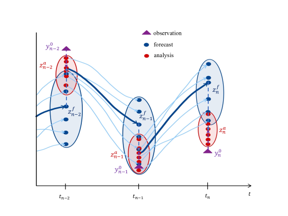
Fig. 3: Illustration of the Ensemble Kalman Filter (EnKF) sequence. The goal of EnKF is to use available observation (purple triangle) to correct the model prediction and get closer to the unknown truth. Blue and red ellipses represent the uncertainty in forecast and assimilated states, respectively. Thin blue lines depict the evolution of ensembles, while the thick blue line traces the average or mean state.

This EnKF procedure is illustrated graphically in Fig. 3, and the process can be summarized compactly as follows: the EnKF forecast ensembles are determined by applying the model to the previous analysis states

$$\bm{\mathrm{z}}_{n+1}^{(m)f}=\mathcal{M}_{n}(\bm{\mathrm{z}}_{n}^{(m)a}),$$

and then the data assimilation step can be written in matrix form as

$$\bm{\mathrm{K}}_{n+1} =\bm{\mathrm{P}}_{n+1}^{f}\bm{\mathrm{H}}_{n+1}^{T}\Big{[}\bm{\mathrm{H}}_{n+1}\bm{\mathrm{P}}_{n+1}^{f}\bm{\mathrm{H}}_{n+1}^{T}+\bm{\mathrm{R}}_{n+1}\Big{]}^{-1},$$

$$\bm{\mathrm{z}}_{n+1}^{(m)a} =\bm{\mathrm{z}}_{n+1}^{(m)f}+\bm{\mathrm{K}}_{n+1}\left(\bm{\mathrm{y}}_{n+1}^{o}-\mathcal{H}_{n+1}(\bm{\mathrm{z}}_{n+1}^{(m)f})\right).$$

Here, $\bm{\mathrm{K}}_{n}$ (with time index shifted by 1 for simplicity) is constructed in terms of the observational error covariance matrix $\bm{\mathrm{R}}_{n}=E[\bm{\eta}_{n}\bm{\eta}_{n}^{T}]$ and the matrix products

$$\bm{\mathrm{P}}_{n}^{f}\bm{\mathrm{H}}_{n}^{T} =\frac{1}{N_{e}-1}\sum_{m=1}^{N_{e}}\left(\bm{\mathrm{z}}_{n}^{(m)f}-\overline{\bm{\mathrm{z}}}_{n}^{f}\right)\left(\mathcal{H}_{n}(\bm{\mathrm{z}}_{n}^{(m)f})-\frac{1}{N_{e}}\sum_{m^{\prime}=1}^{N_{e}}\mathcal{H}_{n}\left(\bm{\mathrm{z}}_{n}^{(m^{\prime})f}\right)\right)^{T},$$

$$\bm{\mathrm{H}}_{n}\bm{\mathrm{P}}_{n}^{f}\bm{\mathrm{H}}_{n}^{T} =\frac{1}{N_{e}-1}\sum_{m=1}^{N_{e}}\left(\mathcal{H}_{n}(\bm{\mathrm{z}}_{n}^{(m)f})-\frac{1}{N_{e}}\sum_{m^{\prime}=1}^{N_{e}}\mathcal{H}_{n}\left(\bm{\mathrm{z}}_{n}^{(m^{\prime})f}\right)\right)\left(\mathcal{H}_{n}(\bm{\mathrm{z}}_{n}^{(m)f})-\frac{1}{N_{e}}\sum_{m^{\prime}=1}^{N_{e}}\mathcal{H}_{n}\left(\bm{\mathrm{z}}_{n}^{(m^{\prime})f}\right)\right)^{T}.$$

The error covariances $\bm{\mathrm{P}}_{n}^{f}$ are propagated implicitly in time through the ensemble forecasts, which is suitable for large-scale problems and avoids any need to linearize the model equations. In contrast, for a single-forecast filter (without ensembles) the covariances would be propagated explicitly through the use of linearized versions of the model and observation operators.

4.2 ETKF formulation

Among the many variants of the EnKF approach [14], we apply a particular deterministic variant known as the Ensemble Transform Kalman Filter (ETKF) that was originally introduced by Bishop et al. [2]. The key to the ETKF method is defining the analysis covariance matrix $\bm{\mathrm{P}}^{a}$ as a linear transformation of the forecast ensemble perturbation $\bm{\mathrm{Z}}^{f}$. To this end, we first write the forecast ensembles projected onto the observation space in the form of an $N_{y}\times N_{e}$ matrix

$$\left[\bm{\mathrm{y}}_{n}^{(1)f},\;\bm{\mathrm{y}}_{n}^{(2)f},\;\dots,\;\bm{\mathrm{y}}_{n}^{(N_{e})f}\right]=\left[\mathcal{H}_{n}(\bm{\mathrm{z}}_{n}^{(1)f}),\;\mathcal{H}_{n}(\bm{\mathrm{z}}_{n}^{(2)f}),\;\dots,\;\mathcal{H}_{n}(\bm{\mathrm{z}}_{n}^{(N_{e})f})\right],$$

where we recall that $\mathcal{H}$ is the observation operator from (4). These forecast ensembles have mean

$$\overline{\bm{\mathrm{y}}}_{n}^{f}=\frac{1}{N_{e}}\sum_{m=1}^{N_{e}}\bm{\mathrm{y}}_{n}^{(m)f}$$ (27)

and associated associated perturbation matrix

$$\bm{\mathrm{Y}}_{n}^{f}=\left[\left(\bm{\mathrm{y}}_{n}^{(1)f}-\overline{\bm{\mathrm{y}}}_{n}^{f}\right),\;\left(\bm{\mathrm{y}}_{n}^{(2)f}-\overline{\bm{\mathrm{y}}}_{n}^{f}\right),\;\dots,\left(\bm{\mathrm{y}}_{n}^{(N_{e})f}-\overline{\bm{\mathrm{y}}}_{n}^{f}\right)\right].$$ (28)

Next, let $\bm{\mathrm{q}}$ be a vector in $\mathbb{R}^{N_{e}}$ so that $\bm{\mathrm{Z}}_{n}^{f}\bm{\mathrm{q}}$ belongs to the space $\mathbb{R}^{N_{z}}$ spanned by the forecast ensemble perturbation matrix $\bm{\mathrm{Z}}_{n}^{f}$, and let $\bm{\mathrm{z}}_{n}=\overline{\bm{\mathrm{z}}}_{n}^{f}+\bm{\mathrm{Z}}_{n}^{f}\bm{\mathrm{q}}$ be the corresponding model state vector. If $\bm{\mathrm{q}}$ is taken to be a Gaussian random vector with mean $\bm{\mathrm{0}}$ and covariance $(N_{e}-1)^{-1}\bm{\mathrm{I}}$, then $\bm{\mathrm{z}}_{n}=\overline{\bm{\mathrm{z}}}_{n}^{f}+\bm{\mathrm{Z}}_{n}^{f}\bm{\mathrm{q}}$ is also Gaussian with mean $\overline{\bm{\mathrm{z}}}_{n}^{f}$ and covariance $\bm{\mathrm{P}}_{n}^{f}=\frac{1}{N_{e}-1}\bm{\mathrm{Z}}_{n}^{f}(\bm{\mathrm{Z}}_{n}^{f})^{T}$. Following [21, 23] we make the linear approximation

$$\mathcal{H}\Big{(}\overline{\bm{\mathrm{z}}}_{n}^{f}+\bm{\mathrm{Z}}_{n}^{f}\bm{\mathrm{q}}\Big{)}\approx\overline{\bm{\mathrm{y}}}_{n}^{f}+\bm{\mathrm{Y}}_{n}^{f}\bm{\mathrm{q}}$$

in order to construct a cost function to use in finding an optimal choice for $\bm{\mathrm{q}}$. The ETKF analysis step then corresponds to minimizing the following cost function [23]

$$\mathcal{J}(\bm{\mathrm{q}})=\frac{(N_{e}-1)}{2}\bm{\mathrm{q}}^{T}\bm{\mathrm{q}}+\frac{1}{2}\left(\bm{\mathrm{y}}^{o}-\overline{\bm{\mathrm{y}}}^{f}-\bm{\mathrm{Y}}^{f}\bm{\mathrm{q}}\right)^{T}\bm{\mathrm{R}}^{-1}\left(\bm{\mathrm{y}}^{o}-\overline{\bm{\mathrm{y}}}^{f}-\bm{\mathrm{Y}}^{f}\bm{\mathrm{q}}\right)$$

(dropping the time index $n$ for simplicity) to obtain the minimizer

$$\bm{\mathrm{q}}^{a}=\arg\min_{\bm{\mathrm{q}}}\,\mathcal{J}(\bm{\mathrm{q}})=\widetilde{\bm{\mathrm{P}}}^{a}(\bm{\mathrm{Y}}^{f})^{T}\bm{\mathrm{R}}^{-1}\left(\bm{\mathrm{y}}^{o}-\overline{\bm{\mathrm{y}}}^{f}\right),$$ (29)

where

$$\widetilde{\bm{\mathrm{P}}}^{a}=\left((N_{e}-1)\bm{\mathrm{I}}+(\bm{\mathrm{Y}}^{f})^{T}\bm{\mathrm{R}}^{-1}\bm{\mathrm{Y}}^{f}\right)^{-1}$$ (30)

is the inverse of the Hessian of $\mathcal{J}$ at the minimizer. In the model state space, the corresponding analysis mean and covariance are given by

$$\overline{\bm{\mathrm{z}}}^{a} =\overline{\bm{\mathrm{z}}}^{f}+\bm{\mathrm{Z}}^{f}\bm{\mathrm{q}}^{a},$$ (31)

$$\bm{\mathrm{P}}^{a} =\bm{\mathrm{Z}}^{f}\widetilde{\bm{\mathrm{P}}}^{a}{(\bm{\mathrm{Z}}^{f})}^{T}.$$ (32)

To initialize the ensemble forecast that will produce the background state for the next analysis step, we have to choose an analysis ensemble whose sample mean and covariance are equal to $\overline{\bm{\mathrm{z}}}^{a}$ and $\bm{\mathrm{P}}^{a}$ respectively. We therefore construct a matrix $\bm{\mathrm{Z}}^{a}$ so that the sum of its columns is zero and Eq. (26) holds. To this end, the ensemble mean is updated using the analysis equation (31), whereas the ensemble perturbations are updated using the simple linear transformation [2]

$$\bm{\mathrm{Z}}^{a}=\bm{\mathrm{Z}}^{f}\bm{\mathrm{Q}}^{a},$$

where the ensemble transform matrix is

$$\bm{\mathrm{Q}}^{a}=\left((N_{e}-1)\widetilde{\bm{\mathrm{P}}}^{a}\right)^{1/2}.$$

It is then straightforward to show that using

$$\widetilde{\bm{\mathrm{P}}}^{a}=(N_{e}-1)^{-1}\bm{\mathrm{Q}}^{a}(\bm{\mathrm{Q}}^{a})^{T}$$

in Eq. (26) satisfies (32), after which the analysis ensemble perturbation matrix can be obtained using

$$\bm{\mathrm{Z}}^{a}=\bm{\mathrm{Z}}^{f}\left((N_{e}-1)\widetilde{\bm{\mathrm{P}}}^{a}\right)^{1/2}$$ (33)

Finally, the analysis ensemble is formed by adding $\overline{\bm{\mathrm{z}}}^{a}$ to each column of $\bm{\mathrm{Z}}^{a}$ using

$$\bm{\mathrm{z}}^{(m)a}=\overline{\bm{\mathrm{z}}}^{a}+\bm{\mathrm{Z}}^{(m)a},$$ (34)

for $m=1,2,\dots,N_{e}$, after which we may then proceed to the next forecast step by evolving the nonlinear model (21).

5 The SSA–LSM–ETKF algorithm

We now present the SSA–LSM–ETKF procedure described in the previous three sections in algorithmic form, which combines the SSA–LSM algorithm for evolving the ice sheet velocity and interface along with the ETKF algorithm for assimilating observations. Assuming that measurements of surface elevation and terminus position are available at a discrete set of analysis times, we begin by defining the level set function for each initial ensemble. Starting from the state vector $\bm{\mathrm{z}}_{n}$ at time $t_{n}$ (which contains the terminus position and ice thicknesses along the glacier flow line), the forecast step proceeds by integrating the nonlinear model (21) for each ensemble over a single time step. At each analysis time, the data assimilation phase applies the ETKF scheme to generate an analysis state $\bm{\mathrm{z}}^{a}$, after which the level set function is reinitialized for each ensemble. This forecast–assimilation cycle is expanded in detail below:

1. Initialization step: Build a level set function $\varphi$ for each ensemble using the signed distance function in Eq. (15), which requires computing the shortest distance between each discrete grid point $\bm{\mathrm{x}}_{i,j}$ and the ice interface $\Gamma$. To ensure that $\varphi$ is smooth, a finer spatial grid with 50 regularly-spaced points is used in the interior. To handle the possibility that $\Gamma$ may be non-analytic, cubic spline interpolation is used to generate discrete values of $\Gamma$ on finer grids.

2. Forecast step: For each ensemble, the ice velocities $u$, $w$, speed function $S$, and level set function $\varphi$ are computed on a 2D grid of points, $\bm{\mathrm{x}}_{i,j}$. The ice thickness $H$ and upper surface height $h$ are computed at points $x_{i}$.

   1. Compute velocities $u^{k}$ and $w^{k}$: At each time $t^{k}$, the ice thickness $H^{k}$ and the height of the upper surface $h^{k}$ are known. Use these along with the horizontal derivative of $h^{k}$ (determined using a centered difference approximation) in Eq. (10) to determine $u^{k}$. Then use centered approximations of derivatives in Eq. (9) to determine $w^{k}$.

   2. Compute normal speeds $S^{k}$: Use the ice velocities $(u^{k},w^{k})$ and the given surface mass balance function $\omega$ to determine $S^{k}$ at all grid points inside the ice sheet using Eq. (19). At exterior points, values of $S^{k}$ are determined using the procedure described in Section 3.1.

   3. Compute $\varphi^{k+1}$: The level set function is evolved to the next time step using Eq. (16) and the procedure described in Section 3.2.

   4. Extract $H^{k+1}$: The zero level set is determined with subgrid scale precision as the zero contour line of $\varphi^{k+1}$, which is then used to compute $H^{k+1}$ and $h^{k+1}$. The terminus position $x_{\mathrm{g}}^{k}$ is identified as the point where the zero level set intersects the bottom boundary of the domain.

   5. Inner time-stepping loop: Set $t^{k+1}=t^{k}+\Delta t$, increment $k$ and return to Step 2.1, until the next analysis time $t_{n+1}$.

3. Data assimilation step: At each analysis time $t_{n}$ when observations are available, the ETKF procedure combines forecast ensemble states $\bm{\mathrm{z}}^{(m)f}$ (consisting of ice thickness and terminus position) with observations $\bm{\mathrm{y}}^{o}$ to obtain analysis states $\bm{\mathrm{z}}^{(m)a}$. This ETKF scheme is performed according to the following steps:

   1. Use forecast ensembles of ice thickness and terminus position to determine $\overline{\bm{\mathrm{z}}}^{f}$ and $\bm{\mathrm{Z}}^{f}$ using Eqs. (22) and (23).

   2. Compute the corresponding forecast ensembles projected onto the observation space, $\overline{\bm{\mathrm{y}}}^{f}$ and $\bm{\mathrm{Y}}^{f}$, using (27) and (28).

   3. The analysis procedure is divided into two stages, the first of which updates the analysis state only for the single element corresponding to the terminus position, while holding the ice thickness constant:

      1. Compute $\bm{\mathrm{q}}^{a}$ and $\widetilde{\bm{\mathrm{P}}}^{a}$ from Eqs. (29) and (30).

      2. Compute $\overline{\bm{\mathrm{z}}}^{a}$ using $\bm{\mathrm{q}}^{a}$ and forecasts $\overline{\bm{\mathrm{z}}}^{f}$, $\bm{\mathrm{Z}}^{f}$ in (31).

      3. Compute $\bm{\mathrm{Z}}^{a}$ using $\bm{\mathrm{Z}}^{f}$ and $\widetilde{\bm{\mathrm{P}}}$ in (33).

      4. Compute the analysis ensembles by adding $\overline{\bm{\mathrm{z}}}^{a}$ to each of the columns of $\bm{\mathrm{Z}}^{a}$ using (34).

   4. Update the ice thickness to account for calving at the glacier front in two cases:

      1. If the analysis terminus point is advanced beyond the forecasted ice thickness profile, then extend the ice thickness profile using linear interpolation.

      2. If the analysis terminus point lies inside the forecasted ice profile, then adjust the ice thickness profile by removing all ice downstream of the new terminus position.

   5. In stage two of the analysis procedure, repeat Steps 3.3a–d for the elements corresponding to ice thicknesses, while holding the terminus position constant.

4. Reinitialization step: The analysis ensemble $\bm{\mathrm{z}}^{(m)a}$ defines the ice thickness profile and terminus position for each ensemble. The FMM algorithm from Section 3.2 and [20] is used to rebuild the level set function $\varphi$ for each analysis ensemble $\bm{\mathrm{z}}^{(m)a}$.

5. Outer loop: Return to Step 2 to continue the time integration.

6 Numerical results

We now apply the SSA–LSM–ETKF algorithm just described to three experiments of increasing complexity:

• Experiment 1: An idealized marine outlet glacier undergoing inter-annual advances and retreats in response to a given melt rate that is a simple periodic function of time. This first test is performed without any data assimilation to examine the SSA–LSM component of the model only.

• Experiment 2: A repeat of the first experiment with a more realistic pseudo-random time series for the melt rate forcing. Data assimilation is incorporated using synthetic ensembles determined by perturbing the background state.

• Experiment 3: A more realistic test of the data assimilation algorithm that simulates terminus change at Helheim Glacier, one of Greenland’s largest outlet glaciers. The data assimilation step incorporates actual measurements taken over the period 2001–2006.

Each experiment is described separately in the following three sections.

6.1 Experiment 1: Idealized seasonal ice dynamics, without data assimilation

Here we consider the SSA model coupled with the LSM (as described in Section 5) to track a simple grounded marine ice sheet profile as it advances and retreats in response to a synthetic seasonal melting variation. We ignore any effects of ice melange or tidal flexure on the ice dynamics, and assume that the glacier terminates at a calving front with grounding line position $x=x_{\mathrm{g}}$ so that there is no floating portion of the ice shelf.

6.1.1 Experimental design

Following an example from Krug et al. [29], the ice sheet is given an initial profile with surface height

$$h(x)=h_{0}\left(1-(x/x_{\mathrm{g}})^{4}\right)-(1-\rho/\rho_{\mathrm{w}})b(x)\quad\text{for}\;0\leqslant x\leqslant x_{\mathrm{g}},$$ (35)

which lies on top of bedrock having a constant 1% downward slope described by the function $b(x)=-500-0.01x$ (measured in m). The initial terminus position is at $x_{\mathrm{g}}=5000$ m (where the flotation condition (8) is satisfied) and the glacier surface is fixed on the left boundary at a height $h(0)=200\,\mathrm{m}$ above sea level throughout. This initial ice sheet geometry is shown in Fig. 4. The other constant parameter values are ice density $\rho=900\,\mathrm{kg/m^{3}}$, water density $\rho_{\mathrm{w}}=1000\,\mathrm{kg/m^{3}}$ and $h_{0}=150\,\mathrm{m}$. The basal friction coefficient $C(x)$ from Eq. (6) is specified as a linear function that starts at $1.5\times 10^{-2}\,\mathrm{MPa\,m^{-1/3}\,yr^{1/3}}$ at the up-glacier (left) boundary where $x=0$ m, and decreases in the flow direction to $1.0\times 10^{-2}\,\mathrm{MPa\,m^{-1/3}\,yr^{1/3}}$ at $x=10000\,\mathrm{m}$. The ice softness parameter $A$ is set to $5.6\times 10^{-17}\,\mathrm{Pa^{-3}\,yr^{-1}}$, which is typical of glacial ice rheology at a temperature of $-5^{\circ}$C.

Fig. 4: Initial profile of the idealized marine outlet glacier in Experiment 1.

This experiment has a total duration of 7 years and starts off during the initial 2 years with a constant melt rate of $0.41\,\mathrm{m/day}$, which is applied in order to generate a steady-state ice sheet profile. After that, a periodic annual melt cycle with the following time variation is imposed during each of the remaining 5 years

$$\omega(t)=\left\{\begin{array}[]{ll}0.41,&\mathrm{if}\,\,0\leqslant t\leqslant\frac{5}{12},\\[5.69046pt] 0.41+(1.2-0.41)\sin(3\pi t-5\pi/4),&\mathrm{if}\,\,\frac{5}{12}<t\leqslant\frac{9}{12},\\[5.69046pt] 0.41,&\mathrm{if}\,\,\frac{9}{12}<t\leqslant 1,\end{array}\right.$$ (39)

(measured in m/day). The complete seven-year melting rate time series is pictured in Fig. 5a.

The SSA velocity must be determined on a spatial domain extending from $x=0$ to the grounded calving front, which is discretized on a regular spatial grid with spacing of $\Delta x=50\,\mathrm{m}$. Because the terminus position varies continuously with time, $x_{\mathrm{g}}$ does not necessarily coincide with a grid point; consequently, we perform the velocity solve on the computational domain $[0,\,N_{x}\Delta x]$ where $N_{x}=\left\lfloor{x_{\mathrm{g}}}/{\Delta x}\right\rfloor$ so that the terminus point always lies in the interval $N_{x}\Delta x\leqslant x_{\mathrm{g}}<(N_{x}+1)\Delta x$. A constant velocity of $u_{\mathrm{in}}=8000\,\mathrm{m/yr}$ is imposed on the up-glacier boundary, whereas at the calving front we impose the discrete form of $\frac{\partial u}{\partial x}=\left(\frac{1}{4}A^{1/\alpha}(1-\rho/\rho_{\mathrm{w}})\rho gH\right)^{\alpha}$ at $x=x_{\mathrm{g}}$ using cubic extrapolation when the terminus lies outside the computational domain. The LSM solver employs a spatial domain of size $[0,10000\,\mathrm{m}]\times[0,400\,\mathrm{m}]$ which is discretized at a uniform $200\times 100$ grid of points, ensuring that $\Delta x$ is the same for both LSM and SSA solvers and so the horizontal grid locations interior to the ice region coincide. The coupled system is integrated using a constant time step of $\Delta t=5\times 10^{-4}\,\mathrm{yr}$.

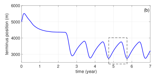
Fig. 5: (a) Prescribed melt rate used as input for Experiment 1. (b) Computed variations in terminus position, with the one-year period $t\in[4.74,5.74]$ highlighted by a dashed box.

6.1.2 Results of seasonal melt forcing

During the start-up period with a constant melt rate the ice sheet experiences a period of relatively rapid advance, reaching its greatest extent of $x_{\mathrm{g}}=5509\,\mathrm{m}$ after 0.14 year. This is simply an artificially induced transient behaviour arising from our initial choice for the upstream glacier height. Following that, the ice sheet retreats and thins, gradually reaching a steady state after roughly 2 years have elapsed (see Fig. 5b). Fig. 6 depicts the corresponding initial ice surface as a black curve, alongside the “steady-state” profile reached after 2 years in green.

After the initial start-up period, the seasonal variations in melt rate pictured in Fig. 5a begin to take place, which causes the ice sheet to experience an annual cycle of advance and retreat. This behaviour can be seen in Fig. 5, where it is easy to connect variations in terminus position with the annual variations in melt rate. The terminus position clearly exhibits a periodic pattern with the same period as the melt rate cycle, varying in extent between $2749.7\,\mathrm{m}$ and $3807.8\,\mathrm{m}$ as measured from the up-glacier domain boundary.

Throughout these annual melting cycles, the ice sheet reaches its minimum extent at times $t=2.76$, 3.74, 4.74, 5.74 and 6.74 years, with the successive maxima occurring at $t=3.42$, 4.42, 5.42 and 6.42 years. The red and blue lines in Fig. 6 picture the advancing/retreating ice profiles at 10 equally-spaced times separated by 0.1 year during the annual period corresponding to $t\in[4.74,5.74]$ (highlighted in the dashed box in Fig. 5b). The red curves show the glacier while advancing and the blue curves during retreat, with the two outermost dash-dot lines representing the maximum and minimum glacier extent. The speed of advance is significantly slower than that for retreat, which is reflected in the fact that more red lines are required to capture the advancing stage. This cycle of slow advance followed by fast retreat is also clearly captured in the plot of terminus position in Fig. 5b where the leading edge of each peak is considerably shallower than the trailing edge. More specifically, the advance from minimum to maximum extent requires approximately 0.68 year, while the subsequent retreat lasts only 0.32 year so that the glacier retreats roughly twice as fast as it advances.

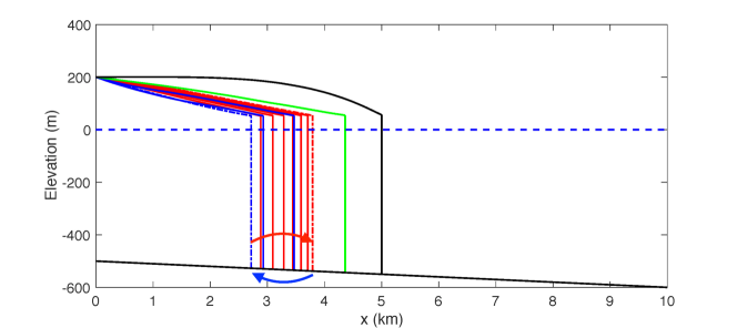
Fig. 6: Variations in glacier surface profile over time for Experiment 1. The black line depicts the initial ice surface from Eq. (35) whereas the green line shows the surface after 2 years of constant melting. Following that, the ice experiences a seasonal cycle of advance and retreat in response to a periodically varying melt rate. The curves corresponding to advance (red) and retreat (blue) are also shown for a single annual cycle at every 0.1 years over the time interval $[4.74,5.74]$.

6.2 Experiment 2: Seasonal ice dynamics with data assimilation

The second experiment is a modified version of Experiment 1 that applies a “pseudo-random” variation in melt rate to more realistically mimic actual weather. We also incorporate the data assimilation portion of the algorithm to illustrate how exploiting observational data within the solution updates can improve accuracy.

6.2.1 Experimental design – Truth run and synthetic observations

We start by generating a model solution using the SSA–LSM algorithm with initial and boundary conditions from Experiment 1, where Eq. (35) is taken as the “true” or reference state for the initial glacier surface, again with $h_{0}=150\,\mathrm{m}$ so that the up-glacier boundary is fixed at $200\,\mathrm{m}$ above the sea level. However, we modify the melt rate forcing from Fig. 5a by applying the constant melt rate $0.41\,\mathrm{m}\,\mathrm{day}^{-1}$ in year 1 only, followed by a seasonal rate that tracks Eq. (39) as a baseline but adds random variability. Because of “pseudo-random” nature of this melt rate, the glacier never reaches a steady state, which is why we only apply the constant melt rate for a single year (compared with 2 years for Experiment 1). The constant melt rate during year 1 also allows us to observe the terminus dynamics in the absence of seasonal melt rate variations. Random variability is incorporated through a linear superposition of 41 Fourier modes of the form $a_{i}\sin(2\pi f_{i}\,t+\phi_{i})$, with frequencies $f_{i}=\frac{i}{6}$ for $i=0,\dots,40$ (where the denominator 6 represents the number of years in this experiment). The amplitude and phase shift for each mode are both chosen randomly from normal distributions, with $a$ having mean 0 and standard deviation 0.025, and $\phi$ with mean 0 and standard deviation $2\pi$. This procedure is used to generate a unique melt rate distribution for the truth run as well as for each ensemble member. In Fig. 7, the true (or reference) melt rate is displayed as a thick blue curve, while the melt rates corresponding to the randomly-generated ensembles lie within the shaded region surrounding this curve. The simulation based on the reference melt rate is considered the “truth run” and is used to measure the quality of our data assimilation estimates.

We next describe the process for generating synthetic observations in the data assimilation process. Based on the truth run described above, we generate randomly perturbed observations by sampling ice surface and terminus position from Gaussian distributions with means equal to the truth values and standard deviations $\sigma_{h}^{\mathrm{obs}}=10\,\mathrm{m}$ and $\sigma_{x_{\mathrm{g}}}^{\mathrm{obs}}=50\,\mathrm{m}$ respectively. Note that this introduces vertical errors in the surface elevation whereas the terminus error is in the horizontal direction. Synthetic observations are generated from the truth run at 10 equally-spaced time intervals each year (for a total of $N_{y}=50$ observations) with samples of surface elevation taken at equidistant points along the flow line with separation distance of $800\,\mathrm{m}$.

Fig. 7: Melt rate time series for the data assimilation Experiment 2. The true/reference melt rate is shown as a solid blue line and the shaded light blue region depicts the spread in melt rates represented by the $N_{e}=50$ ensemble members.

6.2.2 Initial ensembles

There is no well-accepted rule for generating the $N_{e}$ initial ensembles and so we have chosen to employ a common approach [3] that adds Gaussian noise to the background state for the ice surface height. We also introduce an additional horizontal offset by scaling the reference terminus position with a constant factor, replacing $x_{\mathrm{g}}$ with $\lambda x_{\mathrm{g}}$ in Eq. (35). In our EnKF simulations, the ensembles have a mean initial terminus position larger than that for the truth corresponding to $\lambda=1.1$. To generate ensemble values for terminus position $x_{\mathrm{g}}^{(i)}$, we add Gaussian noise to the scaled terminus position $\lambda x_{\mathrm{g}}$ that is sampled from the normal distribution $\mathcal{N}(0,\,\sigma_{\lambda x_{\mathrm{g}}}^{2})$ with standard deviation $\sigma_{\lambda x_{\mathrm{g}}}=50\,\mathrm{m}$. Similarly, the up-glacier surface elevations $h_{0}^{(i)}$ are supplemented with noise sampled from $\mathcal{N}(0,\,\sigma_{h_{0}}^{2})$ with $\sigma_{h_{0}}=10\,\mathrm{m}$. The initial ice surface profile for each ensemble is then generated by replacing (35) with

$$h^{(i)}(x)=h_{0}^{(i)}\left(1-\left(x/{x_{\mathrm{g}}^{(i)}}\right)^{4}\right)-(1-\rho/\rho_{\mathrm{w}})b(x)\quad\text{for}\;0\leqslant x\leqslant x_{\mathrm{g}}^{(i)},$$

for ensembles $i=1,2,\dots,N_{e}$. For this experiment, we generate $N_{e}=50$ ensemble members (consistent with the EnKF approach in [16]) for which our initial ice surface profiles and reference/background states are pictured in Fig. 8. Note that each ensemble is forced using a unique pseudo-random melt rate time series that is different from that of the reference melt rate (see Fig. 7). Furthermore, unlike for the truth run, the surface elevations $h_{0}^{(i)}$ at the up-glacier boundary are not fixed, but instead can vary over time.

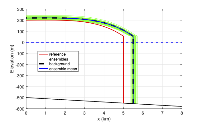
Fig. 8: For Experiment 2, the reference or true ice surface profile is shown in red, the background profile as a dashed black line, the ensemble profiles by green lines, and the ensemble mean in blue.

6.2.3 Results of ETKF simulation with seasonal melt forcing

Using the initial background and ensemble states, we apply the forecast–analysis–reinitialization sequence outlined in the SSA–LSM–ETKF algorithm in Section 5. For comparison purposes, this experiment is repeated using the same initial background states but without data assimilation. Both simulations are subjected to the same pseudo-random melt rate time series described in Section 6.2.1 and pictured in Fig. 7. Note that the ice surface at the up-glacier boundary for this comparison run can also change with time, similar to the data assimilation case.

Between times $t=0$ and $0.1$ yr, we apply the forecast step in Section 5 to predict the ice surface and terminus position for the $N_{e}$ ensembles, with the reference state being used to generate the first set of synthetic observations. The assimilation results from $t=0.1$ are summarised in Fig. 9, where the ensembles of forecast terminus position exhibit a spread between $5765\,\mathrm{m}$ and $6455\,\mathrm{m}$ (refer to Fig. 9a). The analysis step updates the solution as pictured in Fig. 9b, where the terminus observation of $5563.5\,\mathrm{m}$ causes the analysis ensembles to shift into a much tighter range lying between $5542\,\mathrm{m}$ and $5570\,\mathrm{m}$. The mean value of the forecast ensembles is $6080\,\mathrm{m}$, and after the data assimilation step the analysis ensemble mean is $5565\,\mathrm{m}$. Considering that the reference terminus solution is $5537\,\mathrm{m}$, the data assimilation process is clearly successful in moving the ensembles significantly closer to the desired target solution. Likewise, we observe at the up-glacier boundary that the ETKF process also narrows the range of ensemble analysis heights from the forecast range $[188,225]\,\mathrm{m}$ to that of the analysis $[188,210]\,\mathrm{m}$, with the reference/truth value being fixed at $200\,\mathrm{m}$.

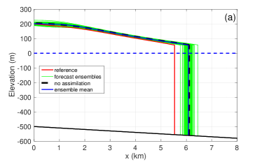
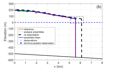
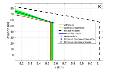
Fig. 9: Solution for Experiment 2 at time $t=0.1$ year. (a) ETKF forecast (before data assimilation) compared with the reference. (b) ETKF analysis (after data assimilation) compared with reference. (c) A zoomed-in view of the boxed region near the terminus highlighted in plot (b). The reference or true ice stream is shown in red, the background as a black dashed line, ensembles in green, and the ensemble average in blue.

We continue applying the forecast–analysis–reinitialization sequence over the full 6-year time period with observational data assimilated every 0.1 yr. After the first full year of the simulation, seasonal melt rate variations begin that drive cycles of ice sheet advance and retreat similar to those observed in Experiment 1. Based on the plot of terminus position in Fig. 10a we observe similar behaviour to the results from Fig. 5, where there is no seasonal melt rate variability during the initial start-up period, after which the terminus position again experiences an approximately periodic pattern of slow advance and rapid retreat. A particularly striking comparison is offered with the simulation without data assimilation which suggests the ice sheet retreats completely after roughly 2.55 years, in stark contrast with the clear cycle of advance/retreat suggested by the data. This is likely due to the fact that the up-glacier boundary height is fixed throughout the entire simulation, whereas the data assimilation algorithm allows the up-glacier height to adjust adaptively with the ensembles in each analysis step.

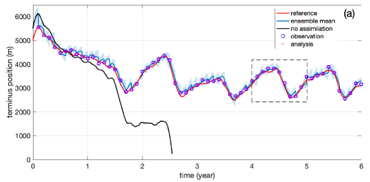
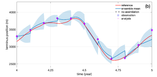
Fig. 10: (a) Time series of terminus positions for Experiment 2. The reference solution is shown as a red line, the ensemble mean in blue, and the ensemble spread by the shaded area. Observation points are available every 0.1 years and shown as circular points. The simulation without data assimilation is shown as a black line. (b) Zoomed-in view of the highlighted area of the terminus plot from plot (a). By focusing in on the time period $[4,5]\;$years, it is much easier to recognize the observation and analysis points and the effect of assimilating observations into the analysis ensembles.

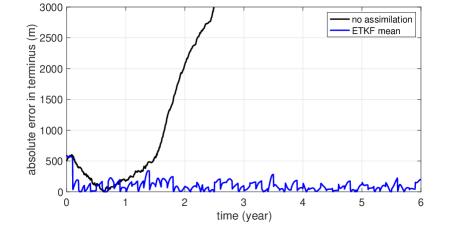
Fig. 11: Mean absolute error in terminus position for Experiment 2, with and without data assimilation.

A zoomed-in view of the terminus plot corresponding to the time period $[4,5]\,\mathrm{yr}$ (highlighted in Fig. 10a) is depicted in Fig. 10b. This plot shows more clearly how the terminus estimate is improved in each data assimilation step and drawn back towards the reference solution. The ETKF procedure provides consistent estimates in the sense that the reference terminus position always lies within the shaded area representing the spread of ensembles. Fig. 11 depicts the evolution of the mean error in terminus position and demonstrates that the ETKF generates reliable forecasts up to the next assimilation time. For example, in the first analysis step at time $t=0.1$ the absolute error in terminus position of the ensemble mean is reduced to $28\,\mathrm{m}$ from the uncorrected value of $546\,\mathrm{m}$, with a similar reduction in every data assimilation step. This well-controlled nature of the ETKF errors should be compared to the errors without data assimilation, shown as black curves in Figs. 10a and 11. Without data assimilation, there is an initial transient reduction in error over the initial time interval $[0,0.635]$, after which the error grows steadily and eventually becomes so large that the glacier retreats completely beyond the up-glacier boundary.

6.3 Experiment 3: Helheim Glacier in Greenland

The final experiment applies our coupled data assimilation algorithm to simulate the motion of Helheim Glacier which is one of the largest outlet glaciers of the Greenland Ice Sheet. The simulated glacier is evolved in time with the SSA–LSM model and remotely-sensed observations of terminus position and surface elevation are incorporated at various times over the period May 2001 to August 2006 using the ETKF. Helheim is a tidewater-terminating glacier that experienced a rapid retreat during the early 2000s followed by a subsequent re-advance (see [22], for example). This period of dramatic ice loss, ice-flow acceleration, and glacier thinning is thought to have resulted from an increase in air temperatures that triggered surface melt-induced thinning and increased basal lubrication, along with increased ocean temperatures that destabilized the glacier terminus [25, 54]. This behaviour has led to the hypothesis that the dynamic mass loss from the Greenland Ice Sheet seen over the past two decades has been triggered largely by perturbations occurring at the terminus of outlet glaciers such as Helheim [55], and it seems likely that Helheim Glacier is set for another period of dramatic retreat [58]. With this in mind, dynamic models that accurately track the terminus position of rapidly changing glaciers are of particular importance for the entire ice sheet [7].

6.3.1 Experimental design

We now describe the configuration of the numerical experiment that will be used to assess the performance of our SSA–LSM–ETKF algorithm. The initial ice geometry is taken from Nick et al. [42] and is based on measured data of glacier surface and bedrock elevations along the near-terminus flow line (see Fig. 12). The horizontal location of the up-glacier boundary is chosen to be $28\,\mathrm{km}$ from the initial terminus. Velocity observations from [42] suggest that horizontal surface velocity at the up-glacier boundary $x=0$ varies between 4.0 and $5.2\,\mathrm{km/yr}$ during the period May 2001 to August 2006. For simplicity, we choose an up-glacier velocity of $u_{\mathrm{in}}$ = $4.5\,\mathrm{km/yr}$ that lies near the middle of this range and is held constant throughout the experiment, which means that the total depth-integrated flux through the up-glacier boundary is constant between observations.

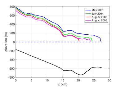
Fig. 12: Bedrock and ice surface profiles for Helheim Glacier, which have been extracted digitally from Nick et al. [42, Fig. 1] using WebPlotDigitizer (https://automeris.io/WebPlotDigitizer).

The computational domain for the SSA velocity solve extends from the up-glacier boundary at $x=0$ to the grounded calving front at $x=x_{\mathrm{g}}$. The left-hand boundary condition is $u(0)=u_{\mathrm{in}}=4.5\,\mathrm{km/yr}$ and a slight modification of the flotation condition (8) is imposed on the right

$$\frac{\partial u(x_{\mathrm{g}})}{\partial x}=C_{F}A\left({\textstyle\frac{1}{4}}\rho(1-\rho/\rho_{\mathrm{w}})gH(x_{\mathrm{g}})\right)^{n},$$

in order to capture the rapid discharge of ice into the ocean. Following [42] we introduce an extra scaling factor $C_{F}$ into Eq. (11), which is a constant front stress perturbation coefficient, with $C_{F}=1$ denoting an unperturbed calving front and $C_{F}>1$ indicating an increased longitudinal strain rate at the terminus position due to rapid discharge (our specific choice for $C_{F}$ is explained in Section 6.3.2).

To capture ice loss due to surface melting we impose a linear variation of net melting rate with distance, increasing from 0 m/yr on the upstream boundary to 40 m/yr at the initial terminus $x=28\,\mathrm{km}$. The basal friction is assigned the constant value $C=3.0\times 10^{-2}\,\mathrm{MPa\,m^{-1/3}\,yr^{1/3}}$, while all other physical parameters are chosen the same as in other experiments (see Table 1). The horizontal and vertical grid spacings for the SSA and LSM discretization are $\Delta x=0.2\,\mathrm{km}$ and $\Delta z=10\,\mathrm{m}$ respectively, and the time step is $\Delta t=5\times 10^{-3}\,\mathrm{yr}$. Finally, within the data assimilation process we incorporate observations of terminus position and surface height (the latter sampled at $2\,\mathrm{km}$ intervals), both of which are extracted from the [42] profiles shown in Fig. 12. These data are then perturbed by random noise sampled from a Gaussian distribution, as explained in the next section.

6.3.2 Initial ensembles

To determine the initial ensembles for Experiment 3, we take the initial background state to be the ice profile observed on May 2001 (see Fig. 12). Ensembles are generated by adding Gaussian noise from $\mathcal{N}(0,\,\sigma^{2})$ to the surface height and choosing terminus positions that satisfy the flotation criteria, which is repeated for $N_{e}=50$ ensemble members with $\sigma=20\,\mathrm{m}$ (see Fig. 13). The flotation criterion is imposed at the terminus for all ensemble members as follows: for any member with surface height lying above the background state, the surface is extrapolated linearly up to the position where the flotation criterion is satisfied; if the surface lies below the background state, then the ice sheet is truncated at the point where flotation criteria is satisfied. Each ensemble is simulated using a different value of the stress perturbation coefficient chosen from the range $[1.5,\,3.5)$, with $C_{F}=1.5+\frac{2}{N_{e}}(i-1)$ for ensembles numbered $i=1,2,\dots,N_{e}$. Note that this range includes the value $C_{F}=2.8$ used by Nick et al. [42] in their modelling studies of Helheim Glacier.

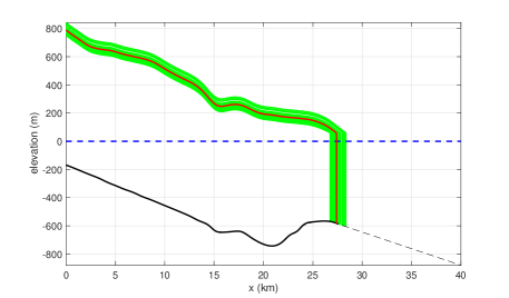
Fig. 13: Initial data for Experiment 3, with the reference or true ice stream in red and the initial ensembles in green.

6.3.3 Tracking ice thickness and terminus for Helheim Glacier

Observational data for surface elevation and terminus position are extracted for this experiment from the measured surface height profiles for Helheim Glacier at three analysis times: July 2004, August 2005 and August 2006 (refer to Fig. 12). For surface elevation we choose equidistant observation points separated by a distance of $2\,\mathrm{km}$ along the flow direction, and add uncorrelated Gaussian noise with zero mean and standard deviation $\sigma_{h}^{\mathrm{obs}}=20\,\mathrm{m}$. A similar process is used to generate observations of the terminus position except that a standard deviation of $\sigma_{x_{\mathrm{g}}}^{\mathrm{obs}}=200\,\mathrm{m}$ is used instead.

Using this data, we may then compute the ice sheet motion by applying the SSA–LSM–ETKF algorithm from Section 5 and performing the forecast–analysis–reinitialization process at the three analysis times. The plots in Figs. 14a–c display the forecast and analysis ensembles on each of these three dates. At the initial time May 2001, we apply the forecast step to predict the ice surface and terminus using $N_{e}$ ensembles. After integrating the SSA model to July 2004, the terminus positions in the forecast ensembles all lie within the range $[24.0,27.0]\,\mathrm{km}$. The corresponding mean terminus position is $26.2\,\mathrm{km}$ which lies $1.9\,\mathrm{km}$ downstream of the observation point. Moving to the ice surface profiles, note that the ensemble elevations encompass the observation point at the up-glacier boundary, with a forecast ranging between $[682.4,737.0]\,\mathrm{m}$ at $x=0$ and with a mean value of $713.7\,\mathrm{m}$.

The algorithm proceeds next to incorporate observations from July 2004 along with the forecast to determine analysis ensembles for ice surface and terminus position. It is clear from Fig. 14a that the ETKF process has contracted the analysis ensembles (in magenta) into a tighter band much closer to the observations. The analysis terminus position lies within the spread of the forecast ensembles, although it has retreated further than most of the forecasts predict. We note also that the forecast ensembles diverge between upward- and downward-sloping portions of the bedrock. At this stage, the level set functions are rebuilt using the FMM and the SSA model integration continues to the next analysis step.

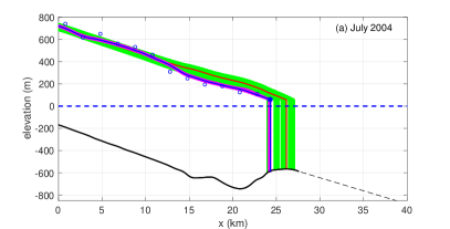
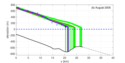
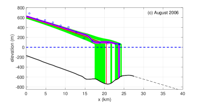
Fig. 14: Forecast and analysis ensembles for Experiment 3 at the three analysis times when observations are assimilated (July 2004, August 2005, August 2006). The green and magenta curves represent forecast and analysis ensembles respectively, and the corresponding means are plotted in red and blue. The ‘$\circ$’ symbol represents ice surface observation points and ‘$\ast$’ the terminus observations.

Upon reaching August 2005 (refer to Fig. 14b) the ensembles exhibit a noticeably larger spread than in the previous step, with the terminus positions ranging between $[20.4,27.0]\,\mathrm{km}$. This demonstrates the inherent uncertainty in the forecast resulting from the nonlinearity of the problem and the sensitivity to slight changes in the bedrock slope at the terminating position as well as the parameter choice $C_{F}$ (which represents buttressing at the terminus). Twelve of the ensembles advance over the bedrock bump and are concentrated on the downward-sloping portion of the bed between $[26.3,27.0]\,\mathrm{km}$, whereas the remaining 38 ensembles retreat (some quite rapidly) and terminate along the upward-sloping portion of the bed. The migration over time of the terminus positions can be seen in Fig. 15, where the mean forecast terminus position on August 2005 is $24.4\,\mathrm{km}$. However, the observed position indicates a dramatic retreat that places the terminus near $x=20.4\,\mathrm{km}$, which coincides with the most rapidly retreating forecasts (at one extreme of the ensemble distribution). This unusually rapid rate of glacier retreat during the 13 months spanning July 2004 to August 2005 (when the observed terminus retreats by $4.1\,\mathrm{km}$, compared to the three-year period from May 2001 to July 2004 when it retreats only $2.8\,\mathrm{km}$) has been the subject of much discussion in the literature (see [22, 25, 54, 55]).

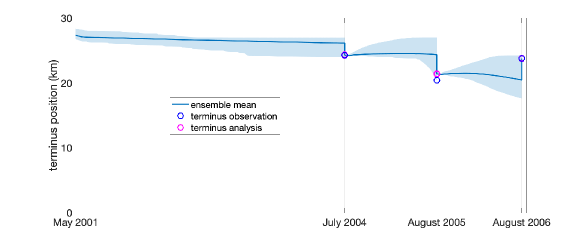
Fig. 15: Terminus positions for Experiment 3, showing the range covered by the ensembles (light blue shaded region), ensemble mean (blue curve) and observation/analysis points (circles).

The data assimilation step succeeds in shifting the simulated terminus back toward the observed retreated location and thereby reducing uncertainty in the solution (see Fig. 15). Focusing again on the up-glacier boundary in Fig. 14b, the simulations yield elevations that are centred around the observation which is similar to the July 2004 analysis step. At lower glacier elevations, the ETKF correction step lowers the ice surface as suggested by the observations. We again reinitialize all ensembles and continue integrating to the final observation point.

Between August 2005 and August 2006, Fig. 14c shows that the forecast again exhibits a strong sensitivity to the initial condition and parameter choice, with some ensembles advancing up the upward sloping bed and others retreating up the downward sloping bed. Observations indicate that Helheim Glacier actually stabilized and re-advanced during this time period, likely in response to an anomalously cold year over Greenland [25]. The data assimilation update, by combining measured observations with the numerical forecast, is shown to address the forecast uncertainties and improve forecasting skill by reinitializing the ice sheet geometry.

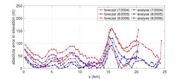
Fig. 16: Absolute error in elevation for the forecast and analysis ensemble means in Experiment 3.

We close by computing the absolute errors in ice sheet elevation for the simulated forecast and analysis means, compared with the observed surface profiles from Fig. 12. These two errors are plotted in Fig. 16 for each analysis time, which shows that the analysis means are more accurate than those for the forecast. Also, the errors within the downward sloping (linear) portion of the bedrock are relatively smaller than those within the non-linear “humped” portion.

7 Conclusion

We developed an algorithm that integrates an Ensemble Transform Kalman Filter (ETKF) data assimilation scheme with an ice-flow model that exploits the level set method to track the ice surface. Accurate simulations of ice sheet-ice stream systems are normally thought to require use of higher order models [28]. However, our hybrid SSA–LSM–ETKF algorithm, using a zeroth-order SSA model, takes special care to accurately capture the terminus position with a LSM and assimilates observational data for both ice surface elevation and terminus position to improve solution fidelity. Based on two idealized marine-terminating glacier experiments and a simulation of the retreat-advance cycle of Helheim Glacier in southeast Greenland, we demonstrate that our data assimilation approach can seamlessly track seasonal and multi-year variability in terminus position and ice surface elevation. This model successfully tracks the ice surface elevation and terminus positions during advance and retreat cycles.

We emphasize that our level set approach allows the terminus position and ice surface to be tracked accurately and efficiently, despite using a simple finite difference discretization on a fixed grid. The LSM approach is robust and should be relatively easy to couple with any ice sheet model from the shallow shelf approximation to a full Stokes flow solver. And even though this paper is restricted to 2D model geometries, it would be straightforward to extend the LSM algorithm to 3D geometries having a dynamically evolving 2D glacier surface and a terminus line. Our data assimilation approach has the additional advantage of being a useful platform for parameter estimation. More specifically, when good estimates are unavailable for model parameters (such as melt rate, front stress perturbation, etc.) we can simply choose a range for each unknown parameter and distribute those values over ensembles, taking advantage of observed data to pinpoint an “optimal” ensemble member. Results of model simulations for experiments on idealized marine-terminating glaciers and Helheim Glacier are encouraging and suggest that this model could be exploited to improve the predictive capability of ice sheet modelling. Marine outlet glaciers (such as Helheim) experience dynamic instabilities due to sensitivity to bed topography and perturbations occurring at ice–atmosphere, ice–ocean, and ice–bed boundaries. The nonlinear response of these glaciers to climate forcing has profound implications for making projections of future mass loss from ice sheets and the resulting sea-level rise. Therefore, numerical techniques such as the one described here could play an important role in efforts to make more accurate predictions of ice mass loss due to climate change.

References

- [1] D. Adalsteinsson and J. A. Sethian. The fast construction of exension velocities in level set methods. Journal of Computational Physics, 148(1):2–22, 1999.
- [2] C. H. Bishop, B. J. Etherton, and S. J. Majumdar. Adaptive sampling with the Ensemble Transform Kalman Filter. Part I: Theoretical aspects. Monthly Weather Review, 129(3):420–436, 2001.
- [3] B. Bonan, N. K. Nichols, M. J. Baines, and D. Partridge. Data assimilation for moving mesh methods with an application to ice sheet modelling. Nonlinear Processes in Geophysics, 24(3):515–534, 2017.
- [4] B. Bonan, M. Nodet, C. Ritz, and V. Peyaud. An ETKF approach for initial state and parameter estimation in ice sheet modelling. Nonlinear Processes in Geophysics, 21(2):569–582, 2014.
- [5] J. H. Bondzio, H. Seroussi, M. Morlighem, T. Kleiner, M. Rückamp, A. Humbert, and E. Y. Larour. Modelling calving front dynamics using a level-set method: Application to Jakobshavn Isbræ, West Greenland. The Cryosphere, 10(2):497–510, 2016.
- [6] E. Bueler and J. Brown. Shallow shelf approximation as a ‘sliding law’ in a thermomechanically coupled ice sheet model. Journal of Geophysical Research: Earth Surface, 114:F03008, 2009.
- [7] G. A. Catania, L. A. Stearns, T. A. Moon, E. M. Enderlin, and R. H. Jackson. Future evolution of Greenland’s marine-terminating outlet glaciers. Journal of Geophysical Research: Earth Surface, 125(2):e2018JF004873, 2020.
- [8] D. Cheng, W. Hayes, E. Larour, Y. Mohajerani, M. Wood, I. Velicogna, and E. Rignot. Calving Front Machine (CALFIN): glacial termini dataset and automated deep learning extraction method for Greenland, 1972-2019. The Cryosphere, 15:1663–1675, 2021.
- [9] G. Cheng, N. Kirchner, and P. Lötstedt. Sensitivity of ice sheet surface velocity and elevation to variations in basal friction and topography in the full Stokes and shallow-shelf approximation frameworks using adjoint equations. The Cryosphere, 15:715–742, 2021.
- [10] N. G. Cogan, F. Bao, R. Paus, and A. Dobreva. Data assimilation of synthetic data as a novel strategy for predicting disease progression in Alopecia areata. Mathematical Medicine and Biology: A Journal of the IMA, 38(3):314–332, 2021.
- [11] K. M. Cuffey and W. S. B. Paterson. The Physics of Glaciers. Academic Press, Cambridge, MA, 2010.
- [12] T. L. Edwards, M. A. Brandon, G. Durand, N. R. Edwards, N. R. Golledge, P. B. Holden, I. J. Nias, A. J. Payne, C. Ritz, and A. Wernecke. Revisiting Antarctic ice loss due to marine ice-cliff instability. Nature, 566:58–64, 2019.
- [13] G. Evensen. Sequential data assimilation with a nonlinear quasi-geostrophic model using Monte Carlo methods to forecast error statistics. Journal of Geophysical Research: Oceans, 99(C5):10143–10162, 1994.
- [14] G. Evensen. The ensemble Kalman filter: Theoretical formulation and practical implementation. Ocean Dynamics, 53(4):343–367, 2003.
- [15] P. Friedl, F. Weiser, A. Fluhrer, and M. H. Braun. Remote sensing of glacier and ice sheet grounding lines: A review. Earth-Science Reviews, 201:102948, 2020.
- [16] F. Gillet-Chaulet. Assimilation of surface observations in a transient marine ice sheet model using an ensemble Kalman filter. The Cryosphere, 14(3):811–832, 2020.
- [17] D. Goldberg and P. Heimbach. Parameter and state estimation with a time-dependent adjoint marine ice sheet model. The Cryosphere, 7:1659–1678, 2013.
- [18] D. N. Goldberg and O. V. Sergienko. Data assimilation using a hybrid ice flow model. The Cryosphere, 5(2):315–327, 2011.
- [19] M. Hoshiba and S. Aoki. Numerical shake prediction for earthquake early warning: Data assimilation, real-time shake mapping, and simulation of wave propagation. Bulletin of the Seismological Society of America, 105(3):1324–1338, 2015.
- [20] M. A. Hossain, S. Pimentel, and J. M. Stockie. Modelling dynamic ice-sheet boundaries and grounding line migration using the level set method. Journal of Glaciology, 66(259):766–776, 2020.
- [21] P. L. Houtekamer and H. L. Mitchell. A sequential ensemble Kalman filter for atmospheric data assimilation. Monthly Weather Review, 129(1):123–137, 2001.
- [22] I. M. Howat, I. Joughin, M. Fahnestock, B. E. Smith, and T. A. Scambos. Synchronous retreat and acceleration of southeast Greenland outlet glaciers 2000-06 ice dynamics and coupling to climate. Journal of Glaciology, 54:646–660, 2008.
- [23] B. R. Hunt, E. J. Kostelich, and I. Szunyogh. Efficient data assimilation for spatiotemporal chaos: A local ensemble transform Kalman filter. Physica D: Nonlinear Phenomena, 230(1-2):112–126, 2007.
- [24] X. Jin, L. Kumar, Z. Li, H. Feng, X. Xu, G. Yang, and J. Wang. A review of data assimilation of remote sensing and crop models. European Journal of Agronomy, 92:141–152, 2018.
- [25] I. Joughin, I. Howat, R. B. Alley, G. Ekstrom, M. Fahnestock, T. Moon, M. Nettles, M. Truffer, and V. C. Tsai. Ice-front variation and tidewater behavior on Helheim and Kangerdlugssuaq glaciers, Greenland. Journal of Geophysical Research: Earth Surface, 113:F01004, 2008.
- [26] E. Kalnay. Atmospheric Modeling, Data Assimilation and Predictability. Cambridge University Press, Cambridge, UK, 2002.
- [27] M. D. King, I. M. Howat, S. G. Candela, M. J. Noh, S. Jeong, B. P. Noël, M. R. van den Broeke, B. Wouters, and A. Negrete. Dynamic ice loss from the Greenland Ice Sheet driven by sustained glacier retreat. Communications Earth & Environment, 1(1):1–7, 2020.
- [28] N. Kirchner, K. Hutter, M. Jakobsson, and R. Gyllencreutz. Capabilities and limitations of numerical ice sheet models: A discussion for Earth-scientists and modelers. Quaternary Science Reviews, 30:3691–3704, 2011.
- [29] J. Krug, G. Durand, O. Gagliardini, and J. Weiss. Modelling the impact of submarine frontal melting and ice mélange on glacier dynamics. The Cryosphere, 9(3):989–1003, 2015.
- [30] K. Law, A. Stuart, and K. Zygalakis. Data Assimilation, volume 62 of Texts in Applied Mathematics. Springer, Cham, Switzerland, 2015.
- [31] J. T. Lenaerts, B. Medley, M. R. van den Broeke, and B. Wouters. Observing and modeling ice sheet surface mass balance. Reviews of Geophysics, 57(2):376–420, 2019.
- [32] L. Li, F.-X. Le Dimet, J. Ma, and A. Vidard. A level-set-based image assimilation method: Potential applications for predicting the movement of oil spills. IEEE Transactions on Geoscience and Remote Sensing, 55(11):6330–6343, 2017.
- [33] D. R. MacAyeal. Large-scale ice flow over a viscous basal sediment: Theory and application to ice stream B, Antarctica. Journal of Geophysical Research: Solid Earth, 94(B4):4071–4087, 1989.
- [34] D. R. MacAyeal. The basal stress distribution of Ice Stream E, Antarctica, inferred by control methods. Journal of Geophysical Research, 97:595–603, 1992.
- [35] P. Macklin and J. Lowengrub. An improved geometry-aware curvature discretization for level set methods: Application to tumor growth. Journal of Computational Physics, 215(2):392–401, 2006.
- [36] V. Mallet, D. E. Keyes, and F. E. Fendell. Modeling wildland fire propagation with level set methods. Computers & Mathematics With Applications, 57(7):1089–1101, 2009.
- [37] J. Mandel, J. D. Beezley, J. L. Coen, and M. Kim. Data assimilation for wildland fires. IEEE Control Systems Magazine, 29(3):47–65, 2009.
- [38] M. L. Martins, S. C. Ferreira Jr, and M. J. Vilela. Multiscale models for the growth of avascular tumors. Physics of Life Reviews, 4(2):128–156, 2007.
- [39] Y. Morishita, S. Murakami, M. Yokoyama, and G. Ueno. Data assimilation system based on integrated transport simulation of large helical device plasma. Nuclear Fusion, 60(5):056001, 2020.
- [40] J. Mouginot, E. Rignot, and B. Scheuchl. Sustained increase in ice discharge from the Amundsen Sea Embayment, West Antarctica, from 1973 to 2013. Geophysical Research Letters, 41:1576–1584, 2014.
- [41] S. S. Nanthakumar, T. Lahmer, X. Zhuang, G. Zi, and T. Rabczuk. Detection of material interfaces using a regularized level set method in piezoelectric structures. Inverse Problems in Science and Engineering, 24(1):153–176, 2016.
- [42] F. M. Nick, A. Vieli, I. M. Howat, and I. Joughin. Large-scale changes in Greenland outlet glacier dynamics triggered at the terminus. Nature Geoscience, 2(2):110–114, 2009.
- [43] S. Osher and R. Fedkiw. Level Set Methods and Dynamic Implicit Surfaces, volume 153 of Applied Mathematical Sciences. Springer Science & Business Media, New York, 2006.
- [44] S. Osher and N. Paragios. Geometric Level Set Methods in Imaging, Vision, and Graphics. Springer Science & Business Media, New York, 2003.
- [45] S. Osher and J. A. Sethian. Fronts propagating with curvature-dependent speed: Algorithms based on Hamilton-Jacobi formulations. Journal of Computational Physics, 79(1):12–49, 1988.
- [46] M. A. Parrish, H. Moradkhani, and C. M. DeChant. Toward reduction of model uncertainty: Integration of Bayesian model averaging and data assimilation. Water Resources Research, 48(3):W03519, 2012.
- [47] F. Pattyn and M. Morlighem. The uncertain future of the Antarctic Ice Sheet. Science, 367(6484):1331–1335, 2020.
- [48] M. Perego, S. Price, and G. Stadler. Optimal initial conditions for coupling ice sheet models to Earth system models. Journal of Geophysical Research: Earth Surface, 119(9):1894–1917, 2014.
- [49] N. Petra, H. Zhu, G. Stadler, T. J. Hughes, and O. Ghattas. An inexact Gauss-Newton method for inversion of basal sliding and rheology parameters in a nonlinear Stokes ice sheet model. Journal of Glaciology, 58:889–903, 2012.
- [50] A. Pralong and M. Funk. A level-set method for modeling the evolution of glacier geometry. Journal of Glaciology, 50(171):485–491, 2004.
- [51] A. A. Robel, H. Seroussi, and G. H. Roe. Marine ice sheet instability amplifies and skews uncertainty in projections of future sea-level rise. Proceedings of the National Academy of Sciences, 116:14887–14892, 2019.
- [52] J. A. Sethian. Level Set Methods and Fast Marching Methods: Evolving Interfaces in Computational Geometry, Fluid Mechanics, Computer Vision, and Materials Science, volume 3 of Cambridge Monographs on Applied and Computational Mathematics. Cambridge University Press, Cambridge, UK, 1999.
- [53] T. Slater, I. R. Lawrence, I. N. Otosaka, A. Shepherd, N. Gourmelen, L. Jakob, P. Tepes, L. Gilbert, and P. Nienow. Review article: Earth’s ice imbalance. The Cryosphere, 15:233–246, 2021.
- [54] F. Straneo, R. G. Curry, D. A. Sutherland, G. S. Hamilton, C. Cenedese, K. Våge, and L. A. Stearns. Impact of fjord dynamics and glacial runoff on the circulation near Helheim Glacier. Nature Geoscience, 45:322–327, 2011.
- [55] F. Straneo, P. Heimbach, O. Sergienko, G. Hamilton, G. Catania, S. Griffies, R. Hallberg, A. Jenkins, I. Joughin, R. Motyka, et al. Challenges to understanding the dynamic response of Greenland’s marine terminating glaciers to oceanic and atmospheric forcing. Bulletin of the American Meteorological Society, 94(8):1131–1144, 2013.
- [56] M. Tedesco. Remote Sensing of the Cryosphere. John Wiley & Sons, Hoboken, NJ, 2014.
- [57] A. Vieli and A. J. Payne. Assessing the ability of numerical ice sheet models to simulate grounding line migration. Journal of Geophysical Research, 110:F01003, 2005.
- [58] J. J. Williams, N. Gourmelen, P. Nienow, C. Bunce, and D. Slater. Helheim Glacier poised for dramatic retreat. Geophysical Research Letters, 48:e2021GL094546, 2021.
- [59] H.-K. Zhao, T. Chan, B. Merriman, and S. Osher. A variational level set approach to multiphase motion. Journal of Computational Physics, 127(1):179–195, 1996.