Neural Optimal Transport

Abstract

We present a novel neural-networks-based algorithm to compute optimal transport maps and plans for strong and weak transport costs. To justify the usage of neural networks, we prove that they are universal approximators of transport plans between probability distributions. We evaluate the performance of our optimal transport algorithm on toy examples and on the unpaired image-to-image translation.

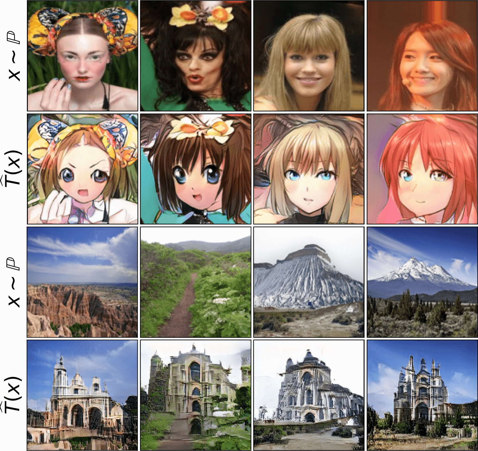
(a) Celeba (female) $\rightarrow$ anime, outdoor $\rightarrow$ church,deterministic (one-to-one, $\mathbb{W}_{2}$).

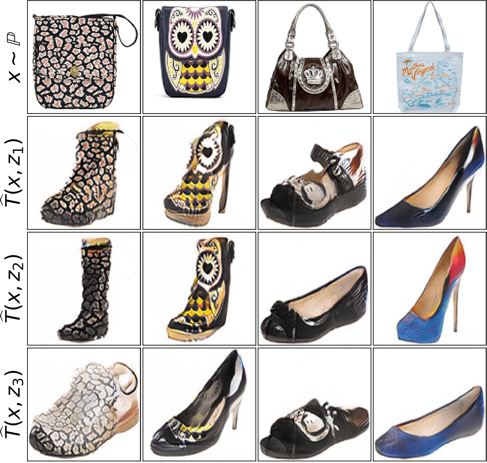
(b) Handbags $\rightarrow$ shoes,stochastic (one-to-many, $\mathcal{W}_{2,1}$).

Figure 1: Unpaired translation with our Neural Optimal Transport (NOT) Algorithm 1.

1 Introduction

Solving optimal transport (OT) problems with neural networks has become widespread in machine learning tentatively starting with the introduction of the large-scale OT (Seguy et al., 2017) and Wasserstein GANs (Arjovsky et al., 2017). The majority of existing methods compute the OT cost and use it as the loss function to update the generator in generative models (Gulrajani et al., 2017; Liu et al., 2019; Sanjabi et al., 2018; Petzka et al., 2017). Recently, (Rout et al., 2022; Daniels et al., 2021) have demonstrated that the OT plan itself can be used as a generative model providing comparable performance in practical tasks.

In this paper, we focus on the methods which compute the OT plan. Most recent methods (Korotin et al., 2021b; Rout et al., 2022) consider OT for the quadratic transport cost (the Wasserstein-2 distance, $\mathbb{W}_{2}$) and recover a nonstochastic OT plan, i.e., a deterministic OT map. In general, it may not exist. (Daniels et al., 2021) recover the entropy-regularized stochastic plan, but the procedures for learning the plan and sampling from it are extremely time-consuming due to using score-based models and the Langevin dynamics (Daniels et al., 2021, 6).

Contributions. We propose a novel algorithm to compute deterministic and stochastic OT plans with deep neural networks (4.1, 4.2). Our algorithm is designed for weak and strong optimal transport costs (2) and generalizes previously known scalable approaches (3, 4.3). To reinforce the usage of neural nets, we prove that they are universal approximators of transport plans (4.4). We show that our algorithm can be applied to large-scale computer vision tasks (5).

Notations. We use $\mathcal{X},\mathcal{Y},\mathcal{Z}$ to denote Polish spaces and $\mathcal{P}(\mathcal{X}),\mathcal{P}(\mathcal{Y}),\mathcal{P}(\mathcal{Z})$ to denote the respective sets of probability distributions on them. We denote the set of probability distributions on $\mathcal{X}\times\mathcal{Y}$ with marginals $\mathbb{P}$ and $\mathbb{Q}$ by $\Pi(\mathbb{P},\mathbb{Q})$. For a measurable map $T:\mathcal{X}\times\mathcal{Z}\rightarrow\mathcal{Y}$ (or $T:\mathcal{X}\rightarrow\mathcal{Y}$), we denote the associated push-forward operator by $T_{\#}$.

2 Preliminaries

In this section, we provide key concepts of the OT theory (Villani, 2008; Santambrogio, 2015; Gozlan et al., 2017; Backhoff-Veraguas et al., 2019) that we use in our paper.

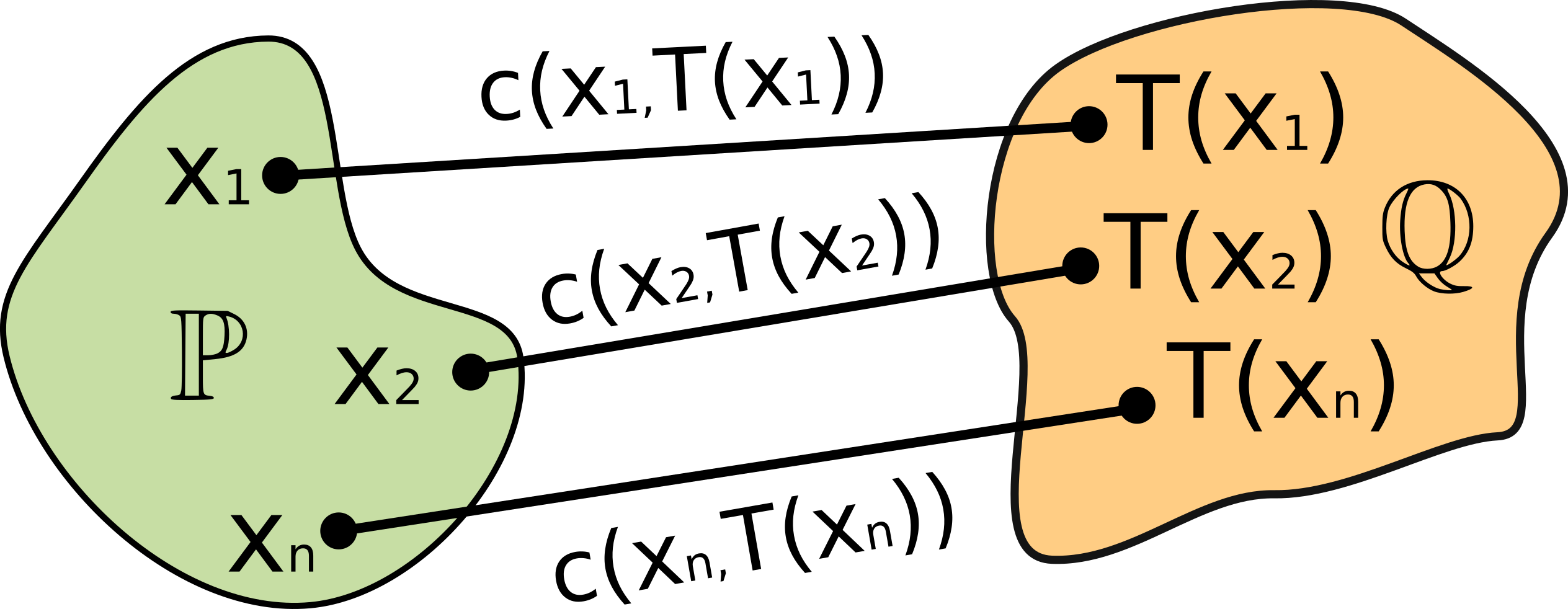
Figure 2: Monge’s OT formulation.

Strong OT formulation. For ${\mathbb{P}\in\mathcal{P}(\mathcal{X})}$, $\mathbb{Q}\in\mathcal{P}(\mathcal{Y})$ and a cost function ${c:\mathcal{X}\times\mathcal{Y}\rightarrow\mathbb{R}}$, Monge’s primal formulation of the OT cost is

$$\text{Cost}(\mathbb{P},\mathbb{Q})\stackrel{{\scriptstyle\text{def}}}{{=}}\inf_{T_{\#}\mathbb{P}=\mathbb{Q}}\ \int_{\mathcal{X}}c\big{(}x,T(x)\big{)}d\mathbb{P}(x),$$ (1)

where the minimum is taken over measurable functions (transport maps) $T:\mathcal{X}\rightarrow\mathcal{Y}$ that map $\mathbb{P}$ to $\mathbb{Q}$ (Figure 2). The optimal $T^{*}$ is called the OT map.

Note that (1) is not symmetric and does not allow mass splitting, i.e., for some ${\mathbb{P},\mathbb{Q}\in\mathcal{P}(\mathcal{X}),\mathcal{P}(\mathcal{Y})}$, there may be no $T$ satisfying $T_{\#}\mathbb{P}=\mathbb{Q}$. Thus, (Kantorovitch, 1958) proposed the following relaxation:

$$\text{Cost}(\mathbb{P},\mathbb{Q})\stackrel{{\scriptstyle\text{def}}}{{=}}\inf_{\pi\in\Pi(\mathbb{P},\mathbb{Q})}\int_{\mathcal{X}\times\mathcal{Y}}c(x,y)d\pi(x,y),\vspace{-1mm}$$ (2)

where the minimum is taken over all transport plans $\pi$ (Figure 3(a)), i.e., distributions on $\mathcal{X}\times\mathcal{Y}$ whose marginals are $\mathbb{P}$ and $\mathbb{Q}$. The optimal $\pi^{*}\in\Pi(\mathbb{P},\mathbb{Q})$ is called the optimal transport plan. If $\pi^{*}$ is of the form $[\text{id},T^{*}]_{\#}\mathbb{P}\in\Pi(\mathbb{P},\mathbb{Q})$ for some $T^{*}$, then $T^{*}$ minimizes (1). In this case, the plan is called deterministic. Otherwise, it is called stochastic (nondeterministic).

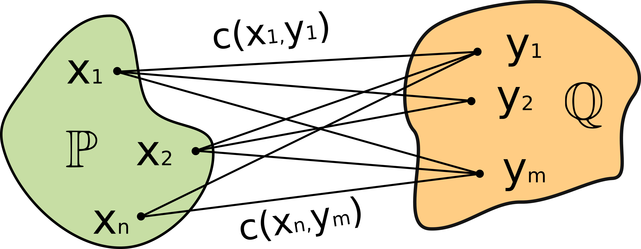
(a) Strong OT formulation (2).

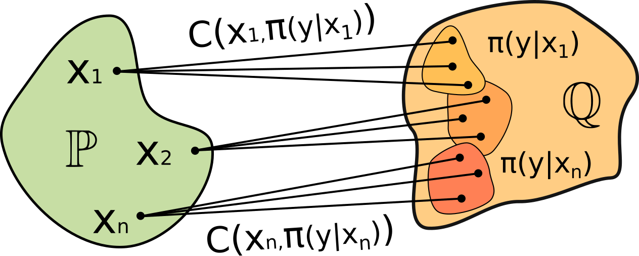
(b) Weak OT formulation (3).

Figure 3: Strong (Kantorovich’s) and weak (Gozlan et al., 2017) optimal transport fomulations.

An example of OT cost for $\mathcal{X}=\mathcal{Y}=\mathbb{R}^{D}$ is the ($p$-th power of) Wasserstein-$p$ distance $\mathbb{W}_{p}$, i.e., formulation (2) with $c(x,y)=\|x-y\|^{p}$. Two its most popular cases are $p=1,2$ ($\mathbb{W}_{1},\mathbb{W}_{2}^{2}$).

Weak OT formulation (Gozlan et al., 2017). Let ${C:\mathcal{X}\times\mathcal{P}(\mathcal{Y})\rightarrow\mathbb{R}}$ be a weak cost, i.e., a function which takes a point $x\in\mathcal{X}$ and a distribution of $y\in\mathcal{Y}$ as input. The weak OT cost between $\mathbb{P},\mathbb{Q}$ is

$$\text{Cost}(\mathbb{P},\mathbb{Q})\stackrel{{\scriptstyle\text{def}}}{{=}}\inf_{\pi\in\Pi(\mathbb{P},\mathbb{Q})}\int_{\mathcal{X}}C\big{(}x,\pi(\cdot|x)\big{)}d\pi(x),\vspace{-1mm}$$ (3)

where $\pi(\cdot|x)$ denotes the conditional distribution (Figure 3(b)). Note that (3) is a generalization of (2). Indeed, for cost $C\big{(}x,\mu\big{)}=\int_{\mathcal{Y}}c(x,y)d\mu(y)$, the weak formulation (3) becomes strong (2). An example of a weak OT cost for $\mathcal{X}=\mathcal{Y}=\mathbb{R}^{D}$ is the $\gamma$-weak ($\gamma\!\geq\!0$) Wasserstein-2 ($\mathcal{W}_{2,\gamma}$):

$$C\big{(}x,\mu\big{)}=\int_{\mathcal{Y}}\frac{1}{2}\|x-y\|^{2}d\mu(y)-\frac{\gamma}{2}\text{Var}(\mu)\vspace{-1mm}$$ (4)

Existence and duality. Throughout the paper, we consider weak costs $C(x,\mu)$ which are lower bounded, convex in $\mu$ and jointly lower semicontinuous in an appropriate sense. Under these assumptions, (Backhoff-Veraguas et al., 2019) prove that the minimizer $\pi^{*}$ of (3) always exists. With mild assumptions on $c$, strong costs satisfy these assumptions. In particular, they are linear w.r.t. $\mu$, and, consequently, convex. The $\gamma$-weak quadratic cost (4) is lower-bounded (for $\gamma\leq 1$) and is also convex since the functional $\text{Var}(\mu)$ is concave in $\mu$. For the costs in view, the dual form of (3) is

$$\text{Cost}(\mathbb{P},\mathbb{Q})=\sup_{f}\int_{\mathcal{X}}f^{C}(x)d\mathbb{P}(x)+\int_{\mathcal{Y}}f(y)d\mathbb{Q}(y),\vspace{-1mm}$$ (5)

where $f$ are the upper-bounded continuous functions with not very rapid growth (Backhoff-Veraguas et al., 2019, Equation 1.2) and $f^{C}$ is the weak $C$-transform of $f$, i.e.

$$f^{C}(x)\stackrel{{\scriptstyle\text{def}}}{{=}}\inf_{\mu\in\mathcal{P}(\mathcal{Y})}\left\{C(x,\mu)-\int_{\mathcal{Y}}f(y)d\mu(y)\right\}.\vspace{-2mm}$$ (6)

Note that for strong costs $C$, the infimum is attained at any ${\mu\in\mathcal{P}(\mathcal{Y})}$ supported on the $\operatorname*{arg\,inf}_{y\in\mathcal{Y}}\{c(x,y)-f(y)\}$ set. Therefore, it suffices to use the strong $c$-transform:

$$f^{C}(x)=f^{c}(x)\stackrel{{\scriptstyle\text{def}}}{{=}}\inf_{y\in\mathcal{Y}}\left\{c(x,y)-f(y)\right\}.$$ (7)

For strong costs (2), formula (5) with (7) is the well known Kantorovich duality (Villani, 2008, 5).

Nonuniqueness. In general, an OT plan $\pi^{*}$ is not unique, e.g., see (Peyré et al., 2019, Remark 2.3).

3 Related Work

In large-scale machine learning, OT costs are primarily used as the loss to learn generative models. Wasserstein GANs introduced by (Arjovsky et al., 2017; Gulrajani et al., 2017) are the most popular examples of this approach. We refer to (Korotin et al., 2022b; 2021b) for recent surveys of principles of WGANs. However, these models are out of scope of our paper since they only compute the OT cost but not OT plans or maps (4.3). To compute OT plans (or maps) is a more challenging problem, and only a limited number of scalable methods to solve it have been developed.

We overview methods to compute OT plans (or maps) below. We emphasize that existing methods are designed only for strong OT formulation (2). Most of them search for a deterministic solution (1), i.e., for a map $T^{*}$ rather than a stochastic plan $\pi^{*}$, although $T^{*}$ might not always exist.

To compute the OT plan (map), (Lu et al., 2020; Xie et al., 2019) approach the primal formulation (1) or (2). Their methods imply using generative models and yield complex optimization objectives with several adversarial regularizers, e.g., they are used to enforce the boundary condition ($T_{\#}\mathbb{P}=\mathbb{Q}$). As a result, the methods are hard to setup since they require careful selection of hyperparameters.

In contrast, methods based on the dual formulation (5) have simpler optimization procedures. Most of such methods are designed for OT with the quadratic cost, i.e., the Wasserstein-2 distance ($\mathbb{W}_{2}^{2}$). An evaluation of these methods is provided in (Korotin et al., 2021b). Below we mention their issues.

Methods by (Taghvaei & Jalali, 2019; Makkuva et al., 2020; Korotin et al., 2021a; c) based on input-convex neural networks (ICNNs, see (Amos et al., 2017)) have solid theoretical justification, but do not provide sufficient performance in practical large-scale problems. Methods based on entropy regularized OT (Genevay et al., 2016; Seguy et al., 2017; Daniels et al., 2021) recover regularized OT plan that is biased from the true one, it is hard to sample from it or compute its density.

According to (Korotin et al., 2021b), the best performing approach is $\lceil\text{MM:R}\rfloor$, which is based on the maximin reformulation of (5). It recovers OT maps fairly well and has a good generative performance. The follow-up papers (Rout et al., 2022; Fan et al., 2022) test extensions of this approach for more general strong transport costs $c(\cdot,\cdot)$ and apply it to compute $\mathbb{W}_{2}$ barycenters (Korotin et al., 2022a). Their key limitation is that it aims to recover a deterministic OT map $T^{*}$ which might not exist.

4 Algorithm for Learning OT Plans

In this section, we develop a novel neural algorithm to recover a solution $\pi^{*}$ of OT problem (3). The following lemma will play an important role in our derivations.

Lemma 1 (Existence of transport maps.).

Let $\mu$ and $\nu$ be probability distributions on $\mathbb{R}^{M}$ and $\mathbb{R}^{N}$. Assume that $\mu$ is atomless. Then there exists a measurable $t\!:\!\mathbb{R}^{M}\!\rightarrow\!\mathbb{R}^{N}$ satisfying $t_{\#}\mu=\nu$.

Proof.

(Santambrogio, 2015, Cor. 1.29) proves the fact for $M\!=\!N$. The proof works for $M\!\neq\!N$. ∎

Throughout the paper we assume that $\mathbb{P},\mathbb{Q}$ are supported on subsets $\mathcal{X}\subset\mathbb{R}^{P}$, $\mathcal{Y}\subset\mathbb{R}^{Q}$, respectively.

4.1 Reformulation of the Dual Problem

First, we reformulate the optimization in $C$-transform (6). For this, we introduce a subset $\mathcal{Z}\subset\mathbb{R}^{S}$ with an atomless distribution $\mathbb{S}$ on it, e.g., $\mathbb{S}=\text{Uniform}\big{(}[0,1]\big{)}$ or $\mathcal{N}(0,1)$.

Lemma 2 (Reformulation of the $C$-transform).

The following equality holds:

$$f^{C}(x)\!=\!\inf_{t}\!\left\{C(x,t_{\#}\mathbb{S})\!-\!\int_{\mathcal{Z}}f\big{(}t(z)\big{)}d\mathbb{S}(z)\!\right\},$$ (8)

where the infimum is taken over all measurable ${t:\mathcal{Z}\rightarrow\mathcal{Y}}$.

Proof.

For all $x\in\mathcal{X}$ and $t:\mathcal{Z}\rightarrow\mathcal{Y}$ we have $f^{C}(x)\!\leq\!C(x,t_{\#}\mathbb{S})-\int_{\mathcal{Z}}f\big{(}t(z)\big{)}d\mathbb{S}(z).$ The inequality is straightforward: we substitute $\mu=t_{\#}\mathbb{S}$ to (6) to upper bound $f^{C}(x)$ and use the change of variables. Taking the infimum over $t$, we obtain

$$f^{C}(x)\!\leq\!\inf_{t}\left\{C(x,t_{\#}\mathbb{S})-\int_{\mathcal{Z}}f\big{(}t(z)\big{)}d\mathbb{S}(z)\right\}.$$ (9)

Now let us turn (9) to an equality. We need to show that $\forall\epsilon>0$ there exists $t^{\epsilon}:\mathcal{Z}\rightarrow\mathcal{Y}$ satisfying

$$f^{C}(x)\!+\!\epsilon\;\geq\;C(x,t^{\epsilon}_{\#}\mathbb{S})\!-\!\int_{\mathcal{Z}}f\big{(}t^{\epsilon}(z)\big{)}d\mathbb{S}(z).$$ (10)

By (6) and the definition of $\inf$, $\exists\mu^{\epsilon}\!\in\!\mathcal{P}(\mathcal{Y})$ such that $f^{C}(x)+\epsilon\geq C(x,\mu^{\epsilon})-\int_{\mathcal{Y}}f(y)d\mu^{\epsilon}(y)$. Thanks to Lemma 1, there exists $t^{\epsilon}:\mathcal{Z}\rightarrow\mathcal{Y}$ such that $\mu^{\epsilon}=t^{\epsilon}_{\#}\mathbb{S}$, i.e., (10) holds true. ∎

Now we use Lemma 2 to get an analogous reformulation of the integral of $f^{C}$ in the dual form (5).

Lemma 3 (Reformulation of the integrated $C$-transform).

The following equality holds:

$$\int_{\mathcal{X}}f^{C}(x)d\mathbb{P}(x)=\inf_{T}\int_{\mathcal{X}}\!\left(\!C\big{(}x,T(x,\cdot)_{\#}\mathbb{S}\big{)}\!-\!\int_{\mathcal{Z}}f\big{(}T(x,z)\big{)}d\mathbb{S}(z)\!\right)\!d\mathbb{P}(x),$$ (11)

where the inner minimization is performed over all measurable functions $T:\mathcal{X}\times\mathcal{Z}\rightarrow\mathcal{Y}$.

Proof.

The lemma follows from the interchange between the infimum and integral provided by the Rockafellar’s interchange theorem (Rockafellar, 1976, Theorem 3A).

The theorem states that for a function $F:\mathcal{A}\times\mathcal{B}\rightarrow\mathbb{R}$ and a distribution $\nu$ on $\mathcal{A}$,

$$\int_{\mathcal{A}}\inf_{b\in\mathcal{B}}F(a,b)d\nu(a)\!=\!\inf_{H:\mathcal{A}\rightarrow\mathcal{B}}\!\int_{\mathcal{A}}F(a,H(a))d\nu(a)$$ (12)

We apply (12), use $\mathcal{A}=\mathcal{X}$, $\nu=\mathbb{P}$, and put $\mathcal{B}$ to be the space of measurable functions $\mathcal{Z}\rightarrow\mathcal{Y}$, and $F(a,b)=C(a,b_{\#}\mathbb{S})\!-\!\int_{\mathcal{Y}}f\big{(}y\big{)}d\big{[}b_{\#}\mathbb{S}\big{]}(y).$ Consequently, we obtain that $\int_{\mathcal{X}}f^{C}(x)d\mathbb{P}(x)$ equals

$$\inf_{H}\!\int_{\mathcal{X}}\!\left(\!C\big{(}x,H(x)_{\#}\mathbb{S}\big{)}\!-\!\int_{\mathcal{Y}}f(y)d\big{[}H(x)_{\#}\mathbb{S}](y)\!\right)\!d\mathbb{P}(x)$$ (13)

Finally, we note that the optimization over functions $H:\mathcal{X}\rightarrow\{t:\mathcal{Z}\rightarrow\mathcal{Y}\}$ equals the optimization over functions ${T:\mathcal{X}\times\mathcal{Z}\rightarrow\mathcal{Y}}$. We put $T(x,z)\!=\$, use the change of variables for $y=T(x,z)$ and derive (11) from (13). ∎

Lemma 3 provides the way to represent the dual form (5) as a saddle point optimization problem.

Corollary 1 (Maximin reformulation of the dual problem).

The following holds:

$$\text{Cost}(\mathbb{P},\mathbb{Q})=\sup_{f}\inf_{T}\mathcal{L}(f,T),$$ (14)

where the functional $\mathcal{L}$ is defined by

$$\mathcal{L}(f,T)\stackrel{{\scriptstyle def}}{{=}}\int_{\mathcal{Y}}f(y)d\mathbb{Q}(y)+\int_{\mathcal{X}}\!\left(\!C\big{(}x,T(x,\cdot)_{\#}\mathbb{S}\big{)}\!-\!\int_{\mathcal{Z}}f\big{(}T(x,z)\big{)}d\mathbb{S}(z)\!\right)\!d\mathbb{P}(x).$$ (15)

Proof.

It suffices to substitute (11) into (5). ∎

We say that functions $T:\mathcal{X}\times\mathcal{Z}\rightarrow\mathcal{Y}$ are stochastic maps. If a map $T$ is independent of $z$, i.e., for all $(x,z)\in\mathcal{X}\times\mathcal{Z}$ we have $T(x,z)\equiv T(x)$, we say the map is deterministic.

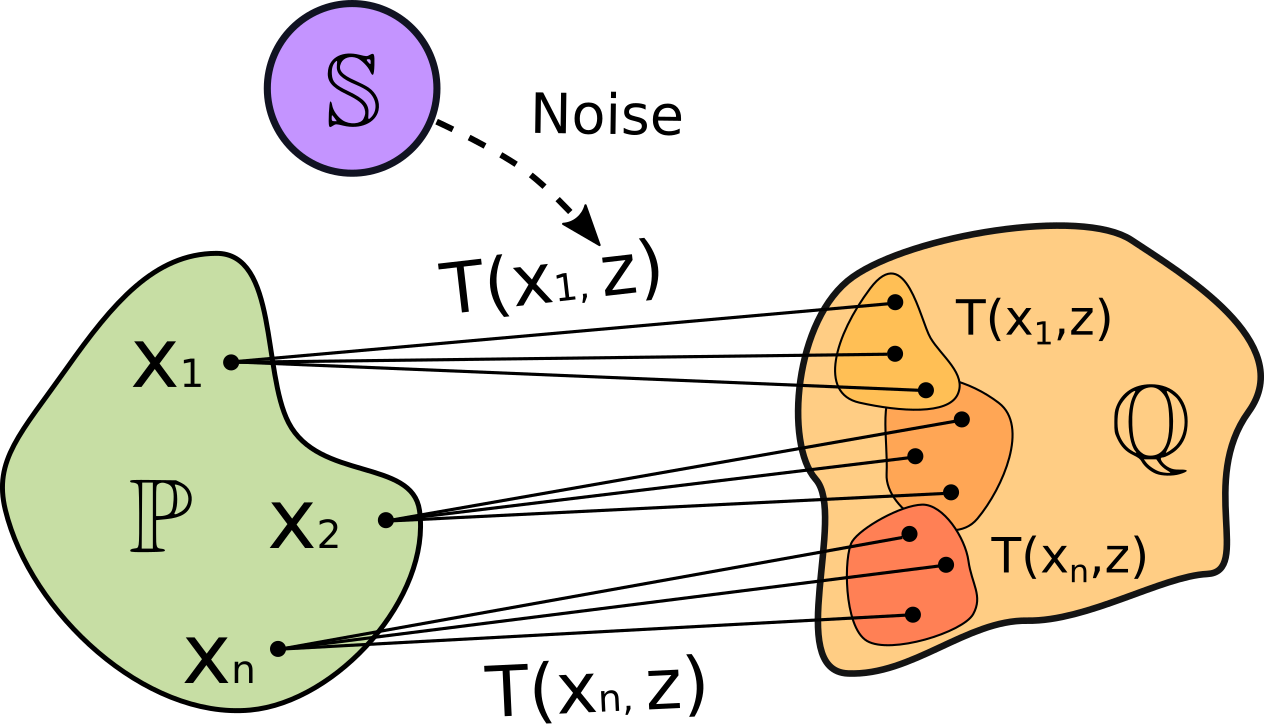
Figure 4: Stochastic function $T(x,z)$ representing a transport plan. The function’s input is $x\in\mathcal{X}$ and $z\sim\mathbb{S}$.

The idea behind the introduced notation is the following. An optimal transport plan $\pi^{*}$ might be nondeterministic, i.e., there might not exist a deterministic function $T:\mathcal{X}\rightarrow\mathcal{Y}$ which satisfies $\pi^{*}=[\text{id}_{\mathcal{X}},T]_{\#}\mathbb{P}$. However, each transport plan $\pi\in\Pi(\mathbb{P},\mathbb{Q})$ can be represented implicitly through a stochastic function ${T:\mathcal{X}\times\mathcal{Z}\rightarrow\mathcal{Y}}$. This fact is known as noise outsourcing (Kallenberg, 1997, Theorem 5.10) for $\mathcal{Z}=[0,1]\subset\mathbb{R}^{1}$ and ${\mathbb{S}=\text{Uniform}([0,1])}$. Combined with Lemma 1, the noise outsourcing also holds for a general $\mathcal{Z}\subset\mathbb{R}^{S}$ and atomless $\mathbb{S}\in\mathcal{P}(\mathcal{Z})$. We visualize the idea in Figure 4. For a plan $\pi$, there might exist multiple maps $T$ which represent it.

For a pair of probability distributions $\mathbb{P},\mathbb{Q}$, we say that $T^{*}$ is a stochastic optimal transport map if it realizes some optimal transport plan $\pi^{*}$. Such maps solve the inner problem in (14) for optimal $f^{*}$.

Lemma 4 (Optimal maps solve the maximin problem).

For any maximizer $f^{*}$ of (5) and for any stochastic map $T^{*}$ which realizes some optimal transport plan $\pi^{*}$, it holds that

$$T^{*}\in\operatorname*{arg\,inf}_{T}\mathcal{L}(f^{*},T).$$ (16)

Proof.

Let $\pi^{*}$ be the OT plan realized by $T^{*}$. We derive

$$\int_{\mathcal{X}}\int_{\mathcal{Z}}f^{*}\big{(}T^{*}(x,z)\big{)}d\mathbb{S}(z)d\mathbb{P}(x)=\int_{\mathcal{X}}\int_{\mathcal{Y}}f^{*}(y)d\pi^{*}(y|x)d\pi^{*}(x)=$$

$$\int_{\mathcal{X}\times\mathcal{Y}}f^{*}(y)d\pi^{*}(x,y)=\int_{\mathcal{Y}}f^{*}(y)d\mathbb{Q}(y),$$ (17)

where we change the variables for $y=T^{*}(x,z)$ and use the property $d\pi^{*}(x)=d\mathbb{P}(x)$. Now assume that $T^{*}\notin\operatorname*{arg\,inf}_{T}\mathcal{L}(f^{*},T)$. In this case, from the definition (15) we conclude that $\mathcal{L}(f^{*},T^{*})>\text{Cost}(\mathbb{P},\mathbb{Q})$. However, we derive substituting (17) into (15), we see that $\mathcal{L}(f^{*},T^{*})=\int_{\mathcal{X}}C\big{(}x,\underbrace{T^{*}(x,\cdot)_{\#}\mathbb{S}}_{\pi^{*}(y|x)}\big{)}\underbrace{d\mathbb{P}(x)}_{d\pi^{*}(x)}\!=\!\text{Cost}(\mathbb{P},\mathbb{Q}),$ which is a contradiction. Thus, (16) holds true. ∎

For the $\gamma$-weak quadratic cost (4) which we use in the experiments (5), a maximizer $f^{*}$ of (5) indeed exists, see (Alibert et al., 2019, 5.22) or (Gozlan & Juillet, 2020). Thanks to our Lemma 16, one may solve the saddle point problem (14) and extract an optimal stochastic transport map $T^{*}$ from its solution $(f^{*},T^{*})$. In general, the $\operatorname*{arg\,inf}$ set for $f^{*}$ may contain not only the optimal stochastic transport maps but other stochastic functions as well. In Appendix F, we show that for strictly convex (in $\mu$) costs $C(x,\mu)$, all the solutions of (14) provide stochastic OT maps.

4.2 Practical Optimization Procedure

To approach the problem (14) in practice, we use neural networks $T_{\theta}:\mathbb{R}^{P}\times\mathbb{R}^{S}\rightarrow\mathbb{R}^{Q}$ and $f_{\omega}:\mathbb{R}^{Q}\rightarrow\mathbb{R}$ to parameterize $T$ and $f$, respectively. We train their parameters with the stochastic gradient ascent-descent (SGAD) by using random batches from $\mathbb{P},\mathbb{Q},\mathbb{S}$, see Algorithm 1.

Input : distributions $\mathbb{P},\mathbb{Q},\mathbb{S}$ accessible by samples; mapping network $T_{\theta}:\mathbb{R}^{P}\times\mathbb{R}^{S}\rightarrow\mathbb{R}^{Q}$;

potential network $f_{\omega}:\mathbb{R}^{Q}\rightarrow\mathbb{R}$; number of inner iterations $K_{T}$;

(weak) cost $C:\mathcal{X}\!\times\!\mathcal{P}(\mathcal{Y})\!\rightarrow\!\mathbb{R}$; empirical estimator $\widehat{C}\big{(}x,T(x,Z)\big{)}$ for the cost;

Output : learned stochastic OT map $T_{\theta}$ representing an OT plan between distributions $\mathbb{P},\mathbb{Q}$;

repeat

     Sample batches $Y\!\sim\!\mathbb{Q}$, $X\sim\mathbb{P}$; for each $x\in X$ sample batch $Z_{x}\sim\mathbb{S}$;

     ${\mathcal{L}_{f}\leftarrow\frac{1}{|X|}\!\sum_{x\in X}\frac{1}{|Z_{x}|}\sum_{z\in Z_{x}}f_{\omega}\!\big{(}T_{\theta}(x,z)\big{)}\!-\!\frac{1}{|Y|}\!\sum_{y\in Y}\!f_{\omega}\!(y)}$;

    

    Update $\omega$ by using $\frac{\partial\mathcal{L}_{f}}{\partial\omega}$;

    

    for $k_{T}=1,2,\dots,K_{T}$ do

         Sample batch $X\sim\mathbb{P}$; for each $x\in X$ sample batch $Z_{x}\sim\mathbb{S}$;

         ${\mathcal{L}_{T}\leftarrow\frac{1}{|X|}\sum_{x\in X}\big{[}\widehat{C}\big{(}x,T_{\theta}(x,Z_{x})\big{)}-\frac{1}{|Z_{x}|}\sum_{z\in Z_{x}}f_{\omega}\big{(}T_{\theta}(x,z)\big{)}\!\big{]}}$;

         Update $\theta$ by using $\frac{\partial\mathcal{L}_{T}}{\partial\theta}$;

        

    

until not converged;

Algorithm 1 Neural optimal transport (NOT)

duct tape

Our Algorithm 1 requires an empirical estimator $\widehat{C}$ for $C\big{(}x,T(x,\cdot)_{\#}\mathbb{S}\big{)}$. If the cost is strong, it is straightforward to use the following unbiased Monte-Carlo estimator from a random batch $Z\sim\mathbb{S}$:

$$C\big{(}x,T(x,\cdot)_{\#}\mathbb{S}\big{)}=\int_{\mathcal{Z}}c(x,T(x,z))d\mathbb{S}(z)\approx\frac{1}{|Z|}\sum_{z\in Z}c\big{(}x,T(x,z)\big{)}\stackrel{{\scriptstyle def}}{{=}}\widehat{C}\big{(}x,T(x,Z)\big{)}.$$ (18)

For general costs $C$, providing an estimator might be nontrivial. For the $\gamma$-weak quadratic cost (4), such an unbiased Monte-Carlo estimator is straightforward to derive:

$$\widehat{C}\big{(}x,T(x,Z)\big{)}\stackrel{{\scriptstyle def}}{{=}}\frac{1}{2|Z|}\sum_{z\in Z}\|x-T(x,z)\|^{2}-\frac{\gamma}{2}\hat{\sigma}^{2},$$ (19)

where $\hat{\sigma}^{2}$ is the (corrected) batch variance $\hat{\sigma}^{2}=\frac{1}{|Z|-1}\sum_{z\in Z}\|T(x,z)-\frac{1}{|Z|}\sum_{z\in Z}T(x,z)\|^{2}.$ To estimate strong costs (18), it is enough to sample a single noise vector ($|Z|=1$). To estimate the $\gamma$-weak quadratic cost (19), one needs $|Z|\geq 2$ since the estimation of the variance $\hat{\sigma}^{2}$ is needed.

4.3 Relation to Prior Works

Generative adversarial learning. Our algorithm 1 is a novel approach to learn stochastic OT plans; it is not a GAN or WGAN-based solution endowed with additional losses such as the OT cost. WGANs (Arjovsky et al., 2017) do not learn an OT plan but use the (strong) OT cost as the loss to learn the generator network. Their problem is $\inf_{T}\sup_{f}\mathcal{V}(T,f)$. The generator $T^{*}$ solves the outer $\inf_{T}$ problem and is the first coordinate of an optimal saddle point $(T^{*},f^{*})$. In our algorithm 1, problem (15) is $\sup_{f}\inf_{T}\mathcal{L}(f,T)$, the generator (transport map) $T^{*}$ solves of the inner $\inf_{T}$ problem and is the second coordinate of an optimal saddle point $(f^{*},T^{*})$. Intuitively, in our case the generator $T$ is adversarial to potential $f$ (discriminator), not vise-versa as in GANs. Theoretically, the problem is also significantly different – swapping $\inf_{T}$ and $\sup_{f}$, in general, yields a different problem with different solutions, e.g., $1\!=\!\inf_{x}\sup_{y}\sin(x\!+\!y)\!\neq\!\sup_{y}\inf_{x}\sin(x\!+\!y)\!=\!-\!1$. Practically, we do $K_{T}>1$ updates of $T$ per one step of $f$, which again differs from common GAN practices, where multiple updates of $f$ are done per a step of $T$. Finally, in contrast to WGANs, we do not need to enforce any constraints on $f$, e.g., the $1$-Lipschitz continuity.

Stochastic generator parameterization. We add an additional noise input $z$ to transport map $T(x,z)$ to make it stochastic. This approach is a common technical instrument to parameterize one-to-many mappings in generative modeling, see (Almahairi et al., 2018, 3.1) or (Zhu et al., 2017b, 3). In the context of OT, (Yang & Uhler, 2019) employ a stochastic generator to learn a transport plan $\pi$ in the unbalanced OT problem (Chizat, 2017). Due to this, their optimization objective slightly resembles ours (15). However, this similarity is deceptive, see Appendix G.

Dual OT solvers. Our algorithm 1 recovers stochastic plans for weak costs (3). It subsumes previously known approaches which learn deterministic OT maps for strong costs (2). When the cost is strong (3) and transport map $T$ is restricted to be deterministic ${T(x,z)\equiv T(x)}$, our Algorithm 1 yields maximin method $\lceil\text{MM:R}\rfloor$, which was discussed in (Korotin et al., 2021b, 2) for the quadratic cost ${\frac{1}{2}\|x-y\|^{2}}$ and further developed by (Rout et al., 2022) for the $Q$-embedded cost ${-\langle Q(x),y\rangle}$ and by (Fan et al., 2022) for other strong costs $c(x,y)$. These works are the most related to our study.

4.4 Universal Approximation with Neural Networks

In this section, we show that it is possible to approximate transport maps with neural nets.

Theorem 1 (Neural networks are universal approximators of stochastic transport maps).

Assume that $\mathcal{X},\mathcal{Z}$ are compact and $\mathbb{Q}$ has finite second moment. Let $T$ be a stochastic map from $\mathbb{P}$ to $\mathbb{Q}$ (not necessarily optimal). Then for any nonaffine continuous activation function which is continuously differentiable at at least one point (with nonzero derivative at that point) and for any $\epsilon>0$, there exists a neural network $T_{\theta}:\mathbb{R}^{P}\times\mathbb{R}^{S}\rightarrow\mathbb{R}^{Q}$ satisfying

$$\|T_{\theta}-T\|^{2}_{L^{2}}\leq\epsilon\qquad\text{and}\qquad\mathbb{W}_{2}^{2}\big{(}(T_{\theta})_{\#}(\mathbb{P}\times\mathbb{S}),\mathbb{Q}\big{)}\leq\epsilon,$$ (20)

where $L^{2}=L^{2}(\mathbb{P}\times\mathbb{S},\mathcal{X}\times\mathcal{Z}\rightarrow\mathbb{R}^{Q})$ is the space of quadratically integrable w.r.t. $\mathbb{P}\times\mathbb{S}$ functions $\mathcal{X}\times\mathcal{Z}\rightarrow\mathbb{R}^{Q}$. That is, the network $T_{\theta}$ generates a distribution which is $\epsilon$-close to $\mathbb{Q}$ in $\mathbb{W}_{2}^{2}$.

Proof.

The squared norm $\|T\|_{L^{2}}^{2}$ is equal to the second moment of $\mathbb{Q}$ since $T$ pushes $\mathbb{P}\times\mathbb{S}$ to $\mathbb{Q}$. The distribution $\mathbb{Q}$ has finite second moment, and, consequently, $T\in L^{2}$. Thanks to (Folland, 1999, Proposition 7.9), the continuous functions ${C^{0}(\mathcal{X}\times\mathcal{Z}\rightarrow\mathbb{R}^{Q})}$ are dense in $L^{2}$. According to (Kidger & Lyons, 2020, Theorem 3.2), the neural networks $\mathbb{R}^{P}\times\mathbb{R}^{S}\rightarrow\mathbb{R}^{Q}$ with the above-mentioned activations are dense in ${C^{0}(\mathcal{X}\times\mathcal{Z}\rightarrow\mathbb{R}^{Q})}$ w.r.t. $L^{\infty}$ norm and, consequently, w.r.t. $L^{2}$ norm. Combining these results yields that neural nets are dense in $L^{2}$, and for every $\epsilon>0$ there necessarily exists network $T_{\theta}$ satisfying the left inequality in (20). For $T_{\theta}$, the right inequality follows from (Korotin et al., 2021a, Lemma A.2). ∎

Our Theorem 1 states that neural nets can approximate stochastic maps in $L^{2}$ norm. It should be taken into account that such continuous nets $T_{\theta}$ may be highly irregular and hard to learn in practice.

5 Evaluation

We perform comparison with the weak discrete OT (considered as the ground truth) on toy 2D, 1D distributions in Appendices B, C, respectively. In this section, we test our algorithm on an unpaired image-to-image translation task. We perform comparison with popular existing translation methods in Appendix D. The code is written in PyTorch framework and is publicly available at

https://github.com/iamalexkorotin/NeuralOptimalTransport

Image datasets. We use the following publicly available datasets as $\mathbb{P},\mathbb{Q}$: aligned anime faces, celebrity faces (Liu et al., 2015), shoes (Yu & Grauman, 2014), Amazon handbags, churches from LSUN dataset (Yu et al., 2015), outdoor images from the MIT places database (Zhou et al., 2014). The size of datasets varies from 50K to 500K images.

Train-test split. We pick 90% of each dataset for unpaired training. The rest 10% are considered as the test set. All the results presented here are exclusively for test images, i.e., unseen data.

Transport costs. We experiment with the strong ($\gamma=0$) and $\gamma$-weak ($\gamma>0$) quadratic costs. Testing other costs, e.g., perceptual (Johnson et al., 2016) or semantic (Cherian & Sullivan, 2019), might be interesting practically, but these two quadratic costs already provide promising performance.

The other training details are given in Appendix E.

5.1 Preliminary Evaluation

In the preliminary experiments with strong cost ($\gamma=0$), we noted that $T(x,z)$ becomes independent of $z$. For a fixed potential $f$ and a point $x$, the map $T(x,\cdot)$ learns to be the map pushing distribution $\mathbb{S}$ to some $\operatorname*{arg\,inf}$ distribution $\mu$ of (6). For strong costs, there are suitable degenerate distributions $\mu$, see the discussion around (7). Thus, for $T$ it becomes unnecessary to keep any dependence on $z$; it simply learns a deterministic map ${T(x,z)=T(x)}$. We call this behavior a conditional collapse.

Importantly, for the $\gamma$-weak cost ($\gamma>0$), we noted a different behavior: the stochastic map $T(x,z)$ did not collapse conditionally. To explain this, we substitute (4) into (3) to obtain

$$\mathcal{W}_{2,\gamma}^{2}(\mathbb{P},\mathbb{Q})=\inf_{\pi\in\Pi(\mathbb{P},\mathbb{Q})}\bigg{[}\int_{\mathcal{X}\times\mathcal{Y}}\frac{1}{2}\|x-y\|^{2}d\pi(x,y)-\gamma\cdot\int_{\mathcal{X}}\frac{1}{2}\text{Var}\big{(}\pi(y|x)\big{)}\underbrace{d\pi(x)}_{d\mathbb{P}(x)}\bigg{]}.\vspace{-0.5mm}$$

The first term is analogous to the strong cost ($\mathbb{W}_{2}=\mathcal{W}_{2,0}$), while the additional second term stimulates the OT plan to be stochastic, i.e., to have high conditional variance.

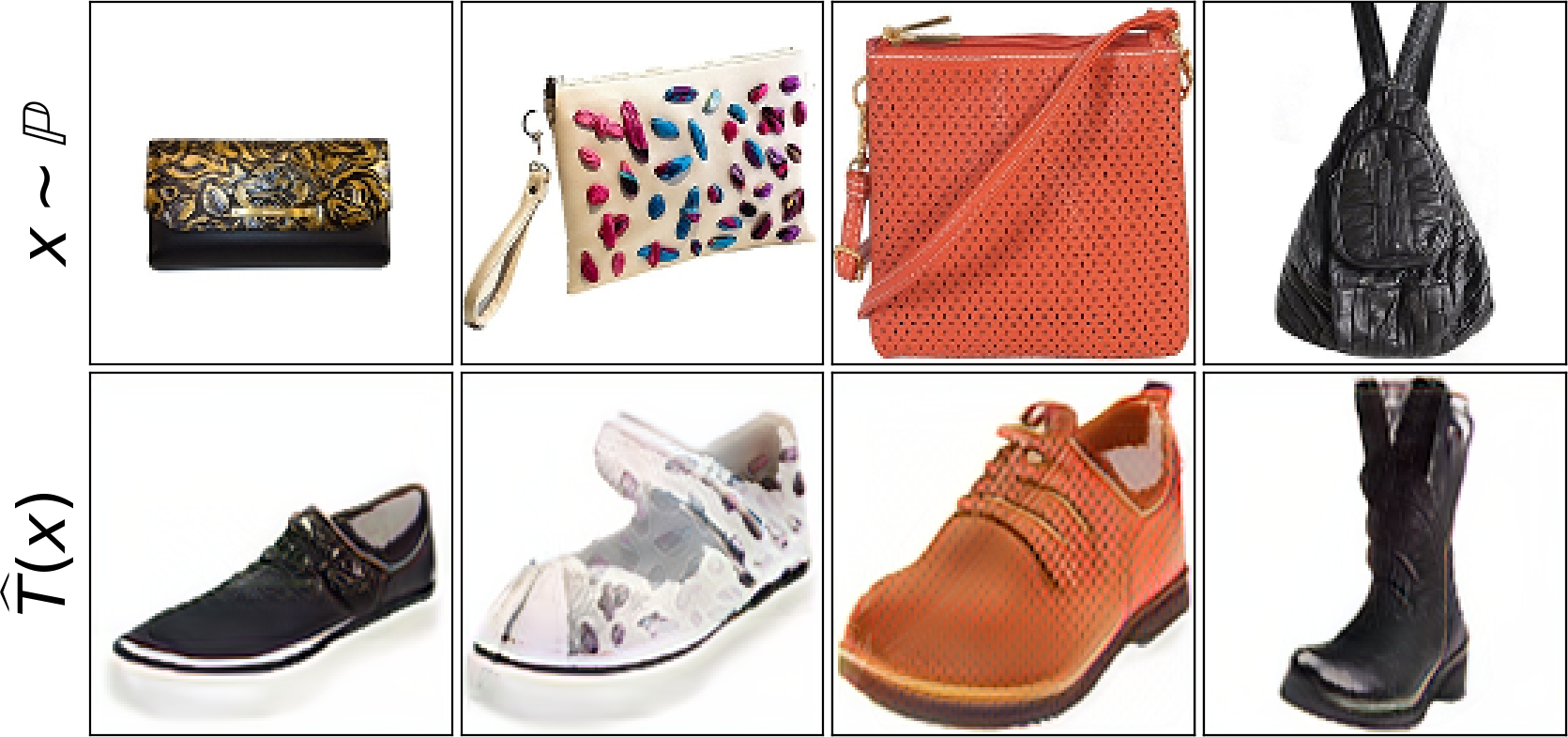
(a) Handbags $\rightarrow$ shoes, $128\times 128$.

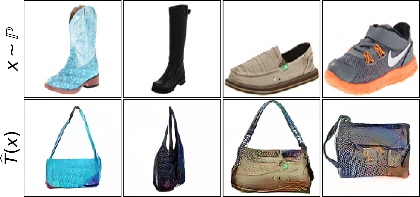
(b) Shoes $\rightarrow$ handbags, $128\times 128$.

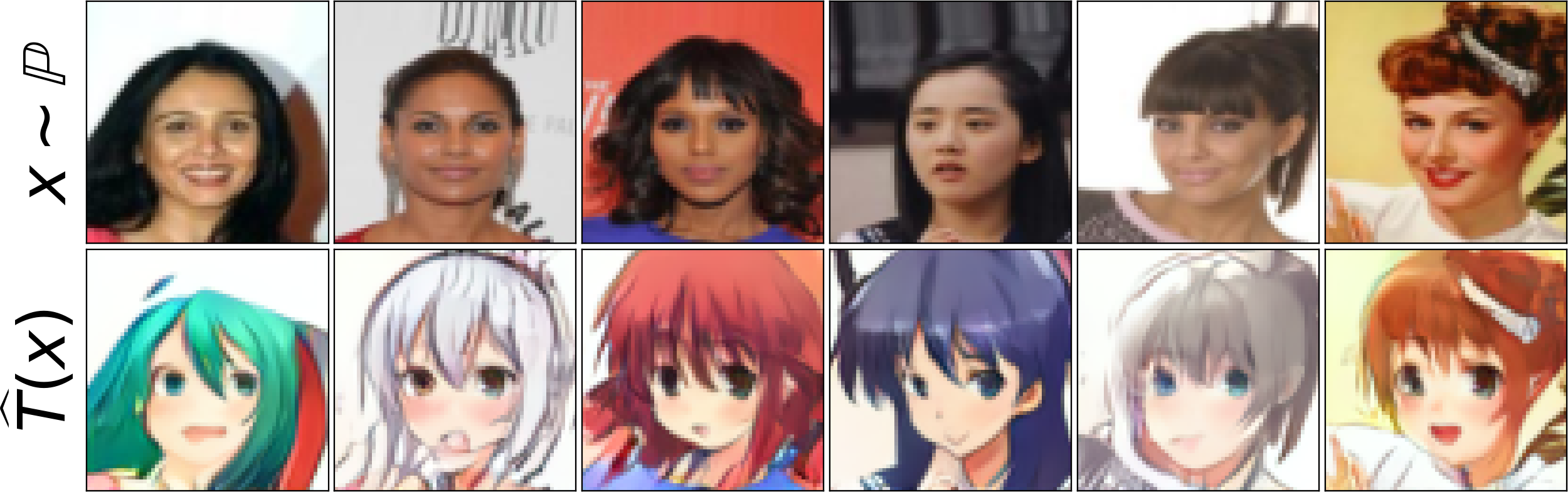
(c) Celeba (female) $\rightarrow$ anime, $64\times 64$.

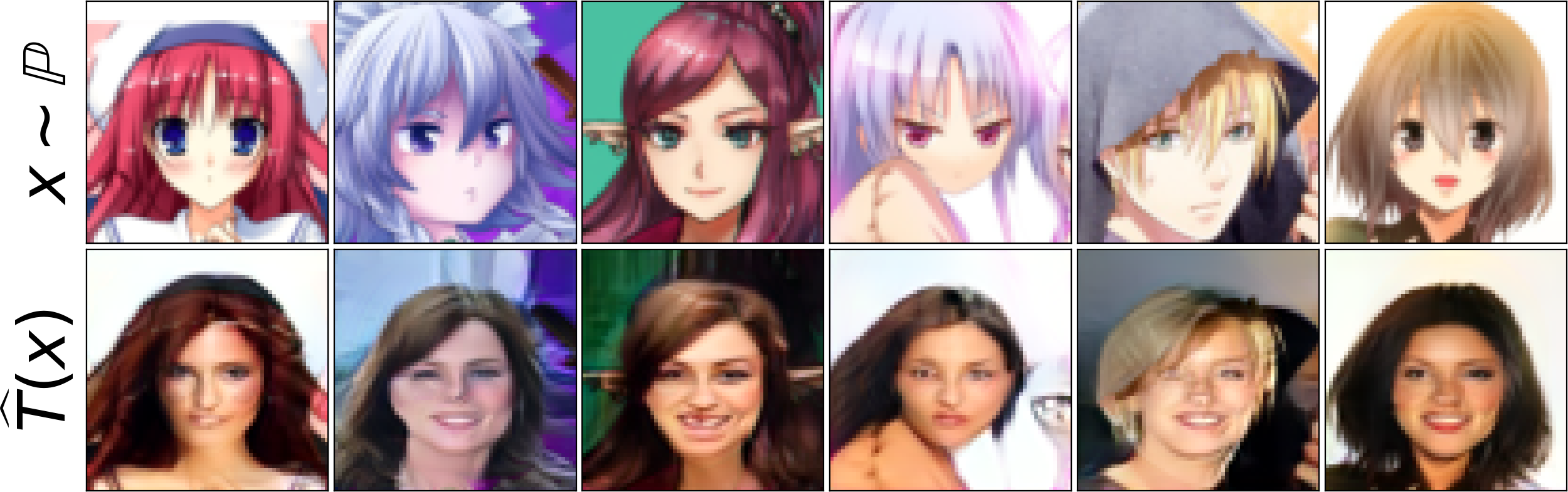
(d) Anime $\rightarrow$ celeba (female), $64\times 64$.

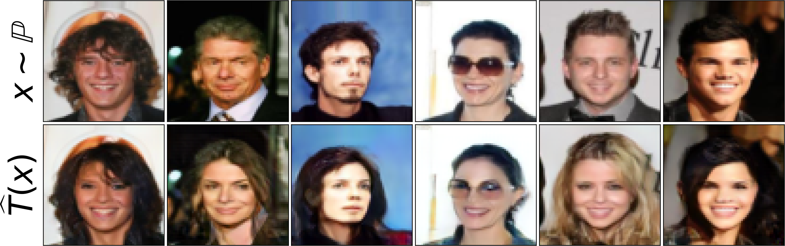
(e) Celeba (male) $\rightarrow$ celeba (female), $64\times 64$.

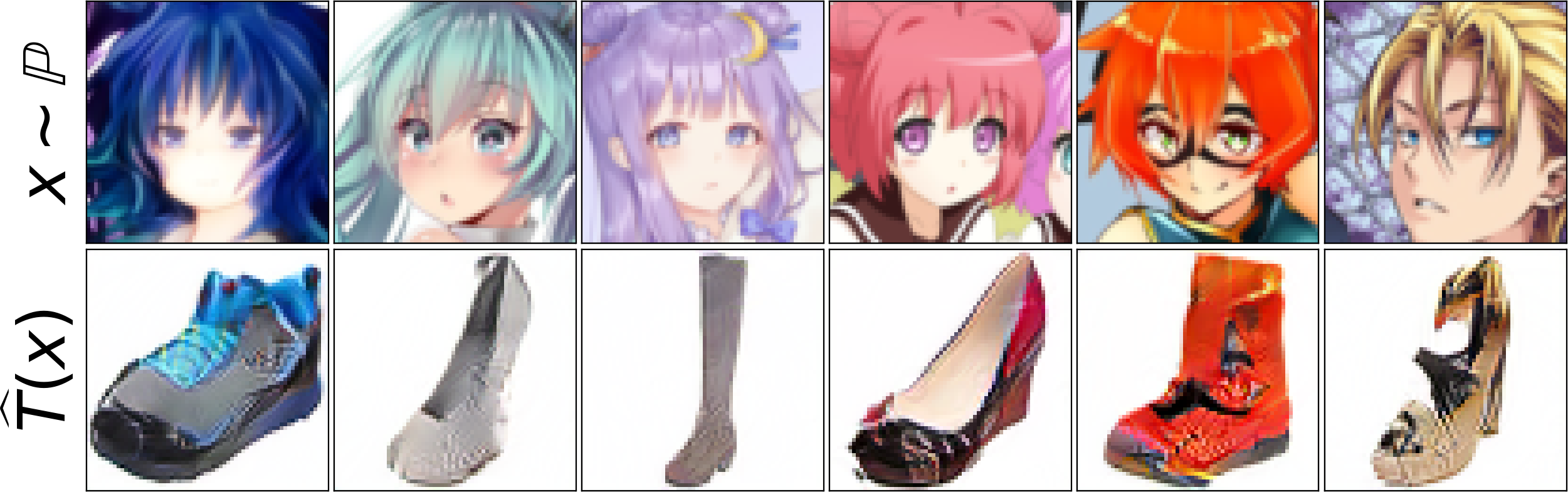
(f) Anime $\rightarrow$ shoes, $64\times 64$.

Figure 5: Unpaired translation with deterministic OT maps ($\mathbb{W}_{2}$).

Taking into account our preliminary findings, we perform two types of experiments. In §5.2, we learn deterministic (one-to-one) translation maps $T(x)$ for the strong cost ($\gamma=0$), i.e., do not add $z$-channel. In §5.3, we learn stochastic (one-to-many) maps $T(x,z)$ for the $\gamma$-weak cost ($\gamma>0$). For completeness, in Appendix A, we study how varying $\gamma$ affects the diversity of samples.

5.2 One-to-one Translation with Optimal Maps

We learn deterministic OT maps between various pairs of datasets. We provide the results in Figures 1(a) and 5. Extra results for all the dataset pairs that we consider are given in Appendix H.

Being optimal, our translation map $\widehat{T}(x)$ tries to minimally change the image content $x$ in the $L^{2}$ pixel space. This results in preserving certain features during translation. In shoes $\leftrightarrow$ handbags (Figures 5(b), 5(a)), the image color and texture of the pushforward samples reflects those of input samples. In celeba (female) $\leftrightarrow$ anime (Figures 1(a), 5(c), 5(d)), head forms, hairstyles are mostly similar for input and output images. The hair in anime is usually bigger than that in celeba. Thus, when translating celeba (female) $\leftrightarrow$ anime, the anime hair inherits the color from the celebrity image background. In outdoor $\rightarrow$ churches (Figure 1(a)), the ground and the sky are preserved, in celeba (male) $\rightarrow$ celeba (female) (Figure 5(e)) – the face does not change. We also provide results for translation in the case when the input and output domains are significantly different, see anime $\rightarrow$ shoes (Figure 5(f)).

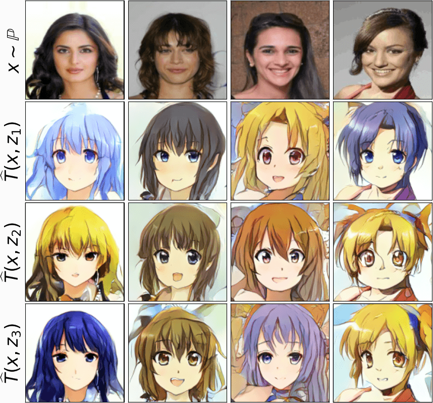
(a) Celeba (female) $\rightarrow$ anime, $128\times 128$ ($\mathcal{W}_{2,\frac{2}{3}}$).

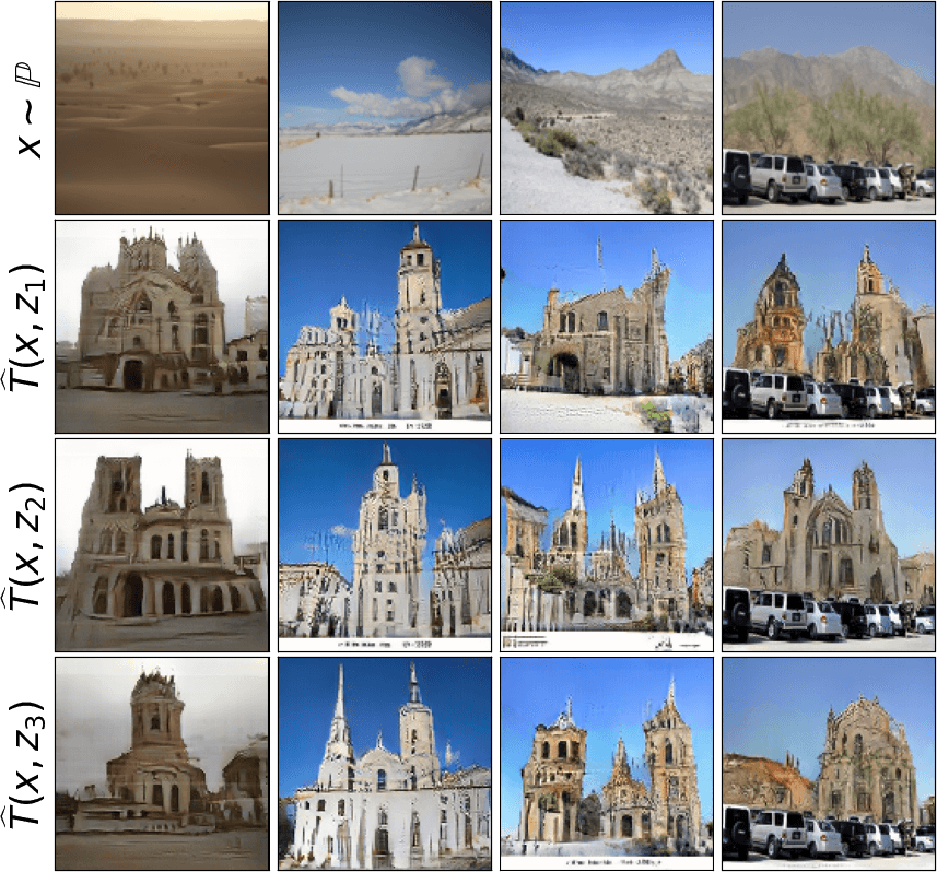
(b) Outdoor $\rightarrow$ church, $128\times 128$ ($\mathcal{W}_{2,\frac{2}{3}}$).

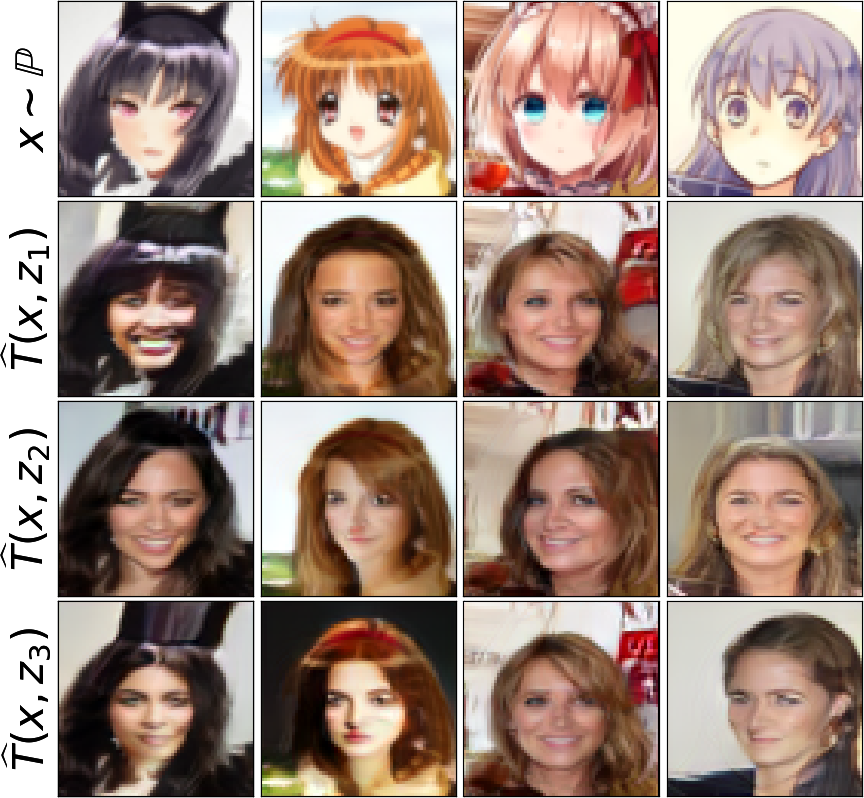
(c) Anime $\rightarrow$ celeba (f), $64\!\times\!64$ ($\mathcal{W}_{2,\frac{2}{3}}$).

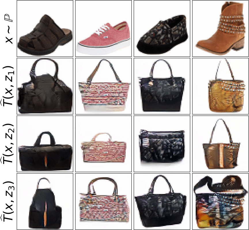
(d) Shoes $\rightarrow$ handbags, $64\times 64$ ($\mathcal{W}_{2,1}$).

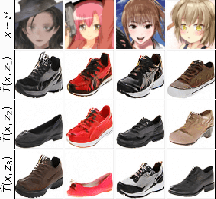
(e) Anime $\rightarrow$ shoes, $64\times 64$ ($\mathcal{W}_{2,1}$).

Figure 6: Unpaired translation with stochastic OT maps ($\mathcal{W}_{2,\gamma}$).

Related work. Existing unpaired translation models, e.g., CycleGAN (Zhu et al., 2017a) or UNIT (Liu et al., 2017), typically have complex adversarial optimization objectives endowed with additional losses. These models require simultaneous optimization of several neural networks. Importantly, vanilla CycleGAN searches for a random translation map and is not capable of preserving certain attributes, e.g., the color, see (Lu et al., 2019, Figure 5b). To handle this issue, imposing extra losses is required (Benaim & Wolf, 2017; Kim et al., 2017), which further complicates the hyperparameter selection. In contrast, our approach has a straightforward objective (14); we use only 2 networks (potential $f$, map $T$), see Table 2 for the comparison of hyperparameters. While the majority of existing unpaired translation models are based on GANs, recent work (Su et al., 2023) proposes a diffusion model (DDIBs) and relates it to Schrödinger Bridge (Léonard, 2014), i.e., entropic OT.

5.3 One-to-many Translation with Optimal Plans

We learn stochastic OT maps between various pairs of datasets for the $\gamma$-weak quadratic cost. The parameter $\gamma$ equals $\frac{2}{3}$ or $1$ in the experiments. We provide the results in Figures 1(b) and 6. In all the cases, the random noise inputs $z\sim\mathbb{S}$ are not synchronized for different inputs $x$. The examples with the synchronized noise inputs $z$ are given in Appendix I. Extended results and examples of interpolation in the conditional latent space are given in Appendix H. The stochastic map $\widehat{T}(x,z)$ preserves the attributes of the input image and produces multiple outputs.

Related work. Transforming a one-to-one learning pipeline to one-to-many is nontrivial. Simply adding additional noise input leads to conditional collapse (Zhang, 2018). This is resolved by AugCycleGAN (Almahairi et al., 2018) and M-UNIT (Huang et al., 2018), but their optimization objectives are much more complicated then vanilla versions. Our method optimizes only $2$ nets $f,T$ in straightforward objective (14). It offers a single parameter $\gamma$ to control the amount of variability in the learned maps. We refer to Table 2 for the comparison of hyperparameters of the methods.

6 Discussion

Potential impact. Our method is a novel generic tool to align probability distributions with deterministic and stochastic transport maps. Beside unpaired translation, we expect our approach to be applied to other one-to-one and one-to-many unpaired learning tasks as well (image restoration, domain adaptation, etc.) and improve existing models in those fields. Compared to the popular models based on GANs (Goodfellow et al., 2014) or diffusion models (Ho et al., 2020), our method provides better interpretability of the learned map and allows to control the amount of diversity in generated samples (Appendix A). It should be taken into account that OT maps we learn might be suitable not for all unpaired tasks. We mark designing task-specific transport costs as a promising research direction.

Limitations. Our method searches for a solution $(f^{*},T^{*})$ of a saddle point problem (14) and extracts the stochastic OT map $T^{*}$ from it. We highlight after Lemma 16 and in 5.1 that not all $T^{*}$ are optimal stochastic OT maps. For strong costs, the issue leads to the conditional collapse. Studying saddle points of (14) and $\operatorname*{arg\,inf}$ sets (16) is an important challenge to address in the further research.

Potential societal impact. Our developed method is at the junction of optimal transport and generative learning. In practice, generative models and optimal transport are widely used in entertainment (image-manipulation applications like adding masks to images, hair coloring, etc.), design, computer graphics, rendering, etc. Our method is potentially applicable to many problems appearing in mentioned industries. While the mentioned applications allow making image processing methods publicly available, a potential negative is that they might transform some jobs in the graphics industry.

Reproducibility. We provide the source code for all experiments and release the checkpoints for all models of 5. The details are given in README.MD in the official repository.

ACKNOWLEDGEMENTS. The work was supported by the Analytical center under the RF Government (subsidy agreement 000000D730321P5Q0002, Grant No. 70-2021-00145 02.11.2021).

Appendix A Variance-Similarity Trade-off

In this section, we study the effect of the parameter $\gamma$ on the structure of the learned stochastic map for the $\gamma$-weak quadratic cost. We consider handbags $\rightarrow$ shoes translation ($64\times 64$) and test $\gamma\in\{0,\frac{1}{3},\frac{2}{3},1\}$. The results are shown in Figure 7.

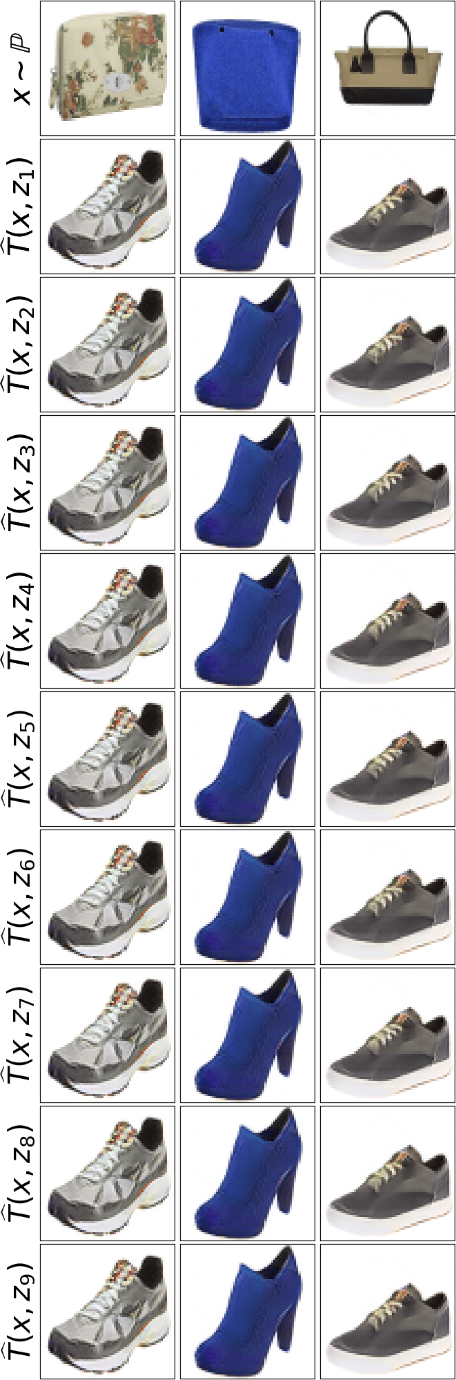
(a) $\gamma=0$

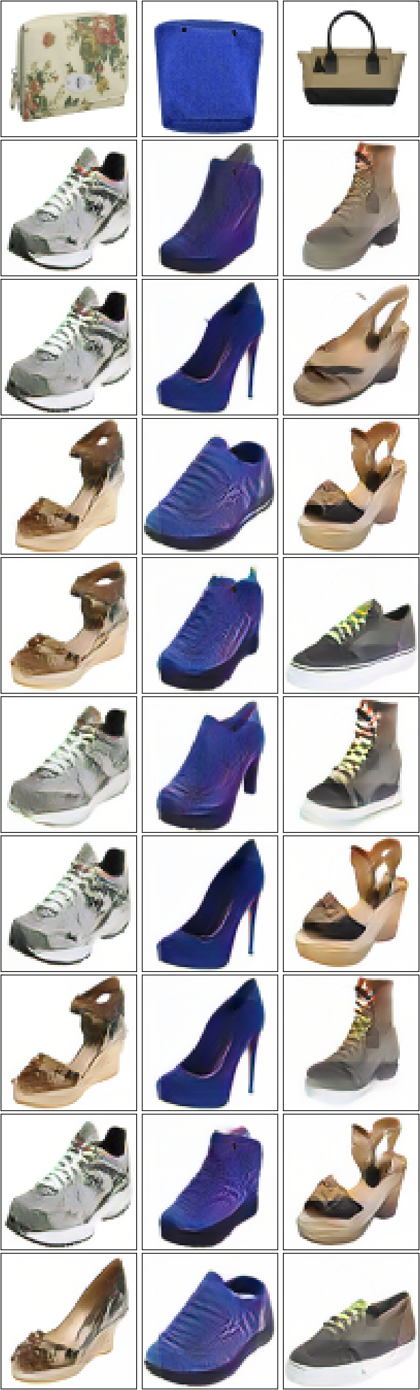
(b) $\gamma=\frac{1}{3}$

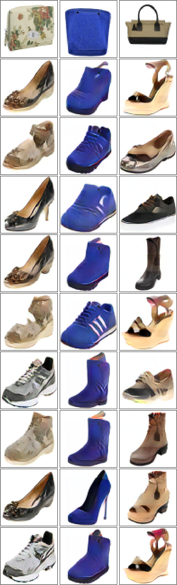
(c) $\gamma=\frac{2}{3}$

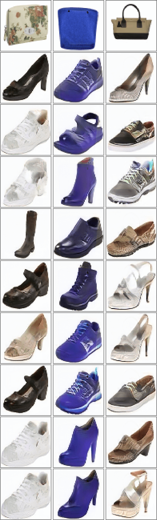
(d) $\gamma=1$

Figure 7: Stochastic Handbags $\rightarrow$ shoes translation with the $\gamma$-weak quadratic cost for various $\gamma$.

Discussion. For $\gamma=0$ there is no variety in produced samples (Figure 7(a)), i.e., the conditional collapse happens. With the increase of $\gamma$ (Figures 7(b), 7(c)), the variety of samples increases and the style of the input images is mostly preserved. For $\gamma=1$ (Figure 7(d)), the variety of samples is very high but many of them do not preserve the style of the input image. The parameter $\gamma$ can be viewed as the trade-off parameter balancing the variance of samples and their similarity to the input.

Appendix B Toy 2D experiments

In this section, we test our Algorithm 1 on toy 2D distributions $\mathbb{P},\mathbb{Q}$, i.e., $P=Q=2$.

Strong quadratic cost ($\gamma=0$). As we noted in 5.1 and Appendix A, for the strong quadratic cost, our method tends to learn deterministic maps $T(x,z)=T(x)$ which are independent of the noise input $z$. For deterministic maps $T(x)$, our method yields $\lfloor\text{MM:R}\rceil$ method which has been evaluated in the recent Wasserstein-2 benchmark by (Korotin et al., 2021b). The authors show that the method recovers OT maps well on synthetic high-dimensional pairs $\mathbb{P},\mathbb{Q}$ with known ground truth OT maps. Thus, for brevity, we do not include toy experiments with our method for the strong quadratic cost.

(a) Input distribution $\mathbb{P}$.

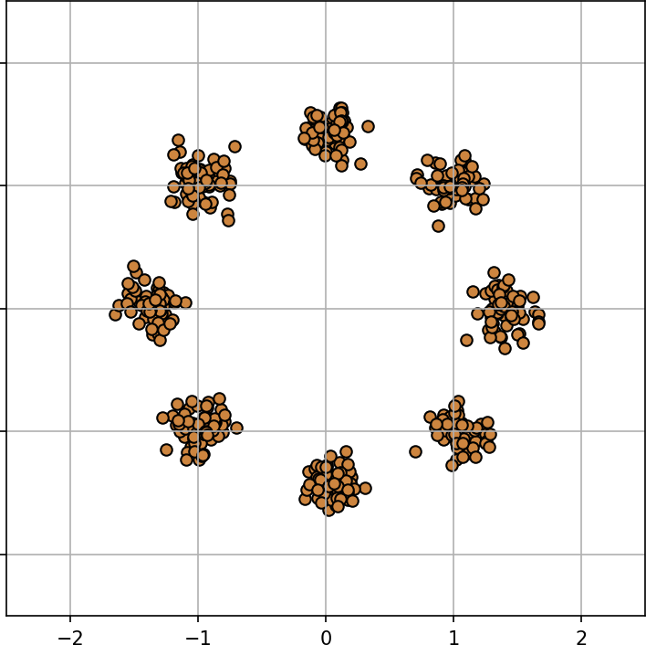
(b) Target distribution $\mathbb{Q}$.

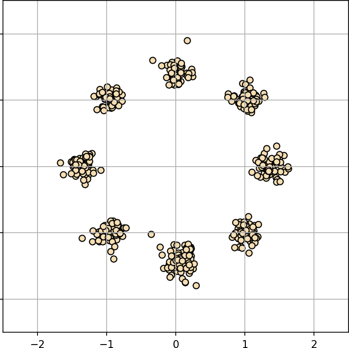
(c) Fitted $\widehat{T}_{\#}(\mathbb{P}\times\mathbb{S})\approx\mathbb{Q}$.

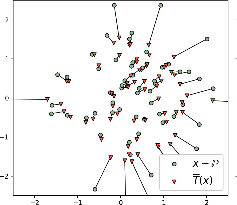
(d) Map $\overline{T}(x)=\int_{\mathcal{Z}}\widehat{T}(x,z)d\mathbb{S}(z)$.

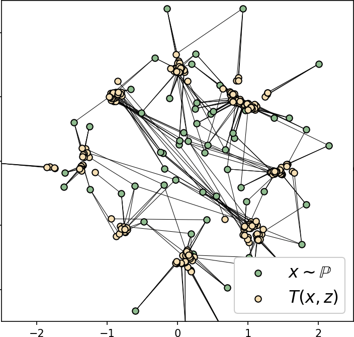
(e) Learned stochastic map $\widehat{T}(x,z)$.

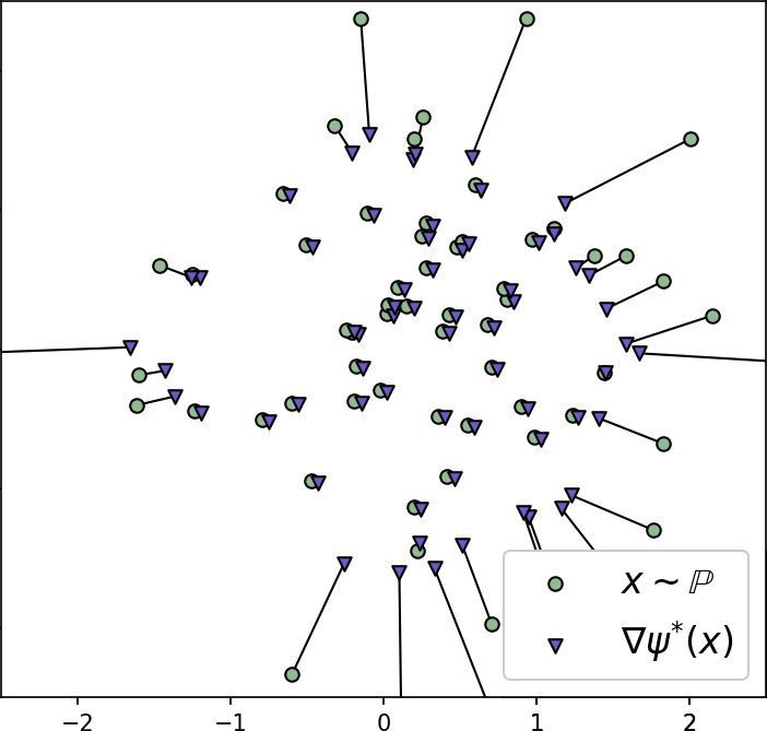
(f) Map $x\!\mapsto\!\int_{\mathcal{Y}}yd\pi^{*}(y|x)$.

Figure 8: Gaussian $\rightarrow$ Mixture of 8 Gaussians, learned stochastic map for the $1$-weak quadratic cost.

Weak quadratic cost ($\gamma>0$). To our knowledge, our method is the first to solve weak OT, i.e., there are no approaches to compare with. The analysis of computed transport plans for weak costs is challenging due to the lack of nontrivial pairs $\mathbb{P},\mathbb{Q}$ with known ground truth OT plan $\pi^{*}$. The situation is even worsened by the nonuniqueness of $\pi^{*}$. To cope with this issue, we consider the weak quadratic cost with $\gamma=1$. For this cost, one may derive

$$C\big{(}x,\mu\big{)}=\int_{\mathcal{Y}}\frac{1}{2}\|x-y\|^{2}d\mu(y)-\frac{1}{2}\text{Var}(\mu)=\frac{1}{2}\|x-\int_{\mathcal{Y}}y\hskip 1.42262ptd\mu(y)\|^{2}.$$ (21)

For cost (21) and a pair $\mathbb{P},\mathbb{Q}$, (Gozlan & Juillet, 2020, Theorem 1.2) states that there exists a $\mathbb{P}$-unique (up to a constant) convex $\psi:\mathbb{R}^{P}\rightarrow\mathbb{R}$ such that every OT plan $\pi^{*}$ satisfies $\nabla\psi(x)=\int_{\mathcal{Y}}y\hskip 2.84526ptd\pi^{*}(y|x)$. Besides, $\nabla\psi:\mathbb{R}^{P}\rightarrow\mathbb{R}^{P}$ is $1$-Lipschitz. Let $\widehat{T}(x,z)$ be the stochastic map recovered by our Algorithm 1, and let $\widehat{\pi}$ be the corresponding plan. Let

$$\overline{T}(x)\stackrel{{\scriptstyle def}}{{=}}\int_{\mathcal{Y}}y\hskip 1.42262ptd\widehat{\pi}(y|x)=\int_{\mathcal{Z}}\widehat{T}(x,z)d\mathbb{S}(z).$$ (22)

Due to the above mentioned characterization of OT plans, $\overline{T}(x)$ should look like a gradient $\nabla\psi(x)$ of some convex function $\psi(x)$ and should nearly be a contraction. Since here we work in the 2D space, we are able to get sufficiently many samples from $\mathbb{P}$ and $\mathbb{Q}$ and obtain a fine approximation of an OT plan $\pi^{*}$ and $\nabla\psi$ by a discrete weak OT solver. We may sample random batches from $X\sim\mathbb{P}$ and $Y\sim\mathbb{Q}$ of size $2^{10}$ and use ot.weak from POT library to get some optimal $\pi^{*}$ and $\nabla\psi=\int_{\mathcal{Y}}y\hskip 2.84526ptd\pi^{*}(y|x)$. We are going to compare our recovered average map $\overline{T}$ with $\nabla\psi$.

Datasets. We test 2 pairs $\mathbb{P},\mathbb{Q}$: Gaussian $\rightarrow$ Mixture of 8 Gaussians; Gaussian $\rightarrow$ Swiss roll.

Neural Networks. We use multi-layer perceptrons as $f_{\omega},T_{\theta}$ with 3 hidden layers of 100 neurons and ReLU nonlinearity. The input of the stochastic map $T_{\theta}(x,z)$ is $2+2=4$ dimensional. The two first dimensions represent the input $x\in\mathbb{R}^{2}$ while the other dimensions represent the noise $z\sim\mathbb{S}$. We employ a Gaussian noise with $\sigma=0.1$

Discussion. We provide qualitative results in Figures 8 and 9. In both cases, the pushforward distribution $\widehat{T}_{\#}(\mathbb{P}\times\mathbb{S})$ matches the desired target distribution $\mathbb{Q}$ (Figures 8(c) and 9(c)). Figures 8(e) and 9(e) show how the mass of points $x\sim\mathbb{P}$ is split by the stochastic map. The average maps $\overline{T}(x)$ (Figures 8(d), 9(d)) indeed nearly match the ground truth $\nabla\psi$ (Figures 8(f), 9(f)) obtained by POT. To quantify them, we compute $\mathcal{L}^{2}$-UVP $(\overline{T})=100\%\cdot\|\overline{T}-\nabla\psi\|^{2}_{\mathbb{P}}/\mbox{Var}(\nabla\psi_{\#}\mathbb{P})$ metric (Korotin et al., 2021a, 5.1). Here we obtain small values $<1\%$ and $\approx 3\%$ for the Swiss Roll and 8 Gaussians examples which further indicates the similarity of the learned $\overline{T}$ and the ground truth $\nabla\psi(x)$.

Note that $\overline{T}$ indeed roughly equals a gradient of a convex function. The gradients of convex functions are cycle monotone (Rockafellar, 1966). Cycle monotonicity yields that for $x_{1}\neq x_{2}$ the segments $[x_{1},\nabla\psi(x_{1})]$ and $[x_{2},\nabla\psi(x_{2})]$ do not intersect in the inner points (Villani, 2008, 8). Visually, we see that in Figures 8(d) and 9(d) the segments $[x,\overline{T}(x)]$ do not intersect for different $x$, which is good.

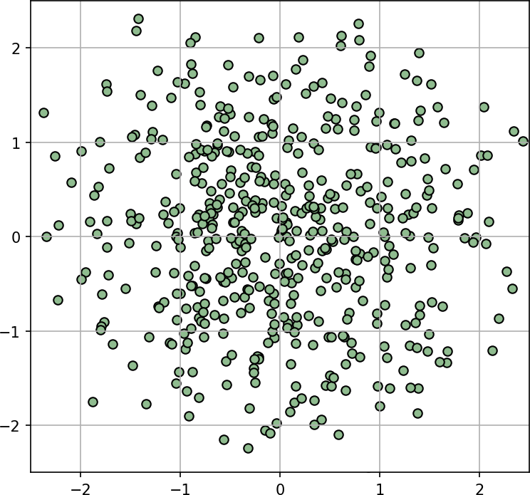
(a) Input distribution $\mathbb{P}$.

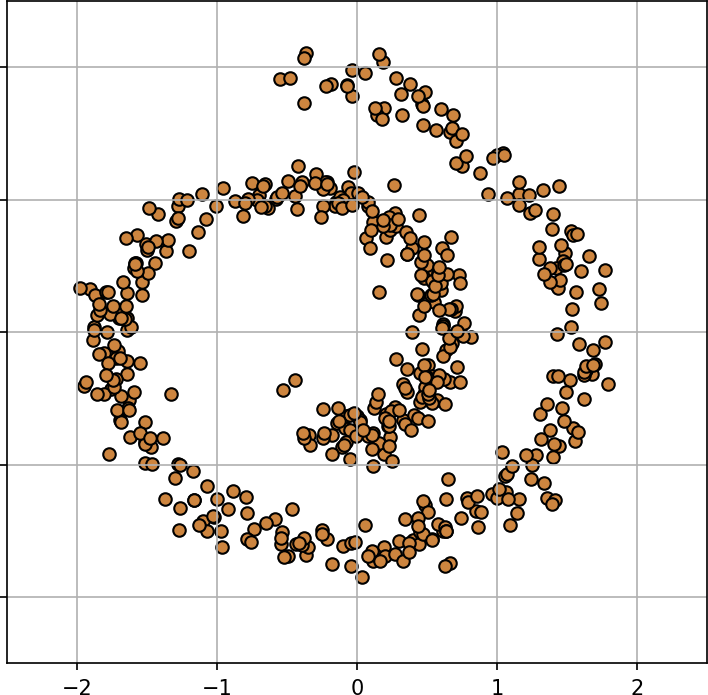
(b) Target distribution $\mathbb{Q}$.

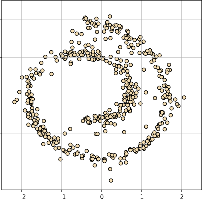
(c) Fitted $\widehat{T}_{\#}(\mathbb{P}\times\mathbb{S})\approx\mathbb{Q}$.

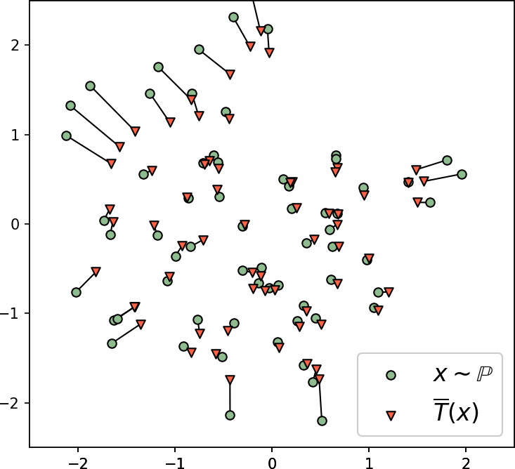
(d) Map $\overline{T}(x)=\int_{\mathcal{Z}}\widehat{T}(x,z)d\mathbb{S}(z)$.

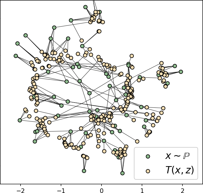
(e) Learned stochastic map $\widehat{T}(x,z)$.

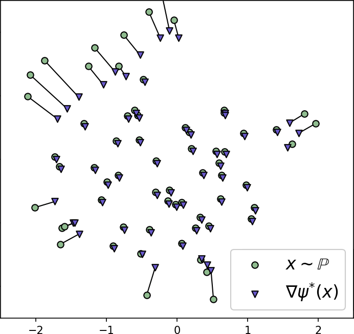
(f) Map $x\!\mapsto\!\int_{\mathcal{Y}}yd\pi^{*}(y|x)$.

Figure 9: Gaussian $\rightarrow$ Swiss Roll, learned stochastic OT map for the $1$-weak quadratic cost.

Appendix C Toy 1D Experiments

In this section, we additionally test our Algorithm 1 on toy 1D distributions $\mathbb{P},\mathbb{Q}$, i.e., $P=Q=1$. In this case, transport plans are 2D distributions and can be conveniently visualized.

We experiment with the $1$-weak quadratic cost (21). Following the discussion in the previous section, we recall that an OT plan $\pi^{*}$ may be not unique. However, all OT plans satisfy ${\nabla\psi(x)=\int_{\mathcal{Y}}y\hskip 2.84526ptd\pi^{*}(y|x)}$ for some 1-smooth convex function $\psi:\mathbb{R}\rightarrow\mathbb{R}$. This simply means that $x\mapsto\nabla\psi(x)=\int_{\mathcal{Y}}y\hskip 2.84526ptd\pi^{*}(y|x)$ is a monotone increasing $1$-Lipschitz function $\nabla\psi:\mathbb{R}\rightarrow\mathbb{R}$. Below we check that this necessary condition holds for $\overline{T}$ (22), where $\hat{T}$ is our learned stochastic map.

Datasets. We test 2 pairs $\mathbb{P},\mathbb{Q}$: Gaussian $\rightarrow$ Mix of 2 Gaussians; Gaussian $\rightarrow$ Mix of 3 Gaussians.

Neural Networks. We use the same networks as in Appendix B. This time, the input of the stochastic map $T_{\theta}(x,z)$ is $1+1=2$ dimensional, the input to $f_{\omega}$ – 1-dimensional.

Discussion. We provide qualitative results in Figures 10 and 11. For each case, we plot the results of 3 random restarts of our method ($\hat{\pi}$ denotes our learned OT plan). Similarly to Appendix B, we plot the results obtained by a discrete weak OT solver (ot.weak from POT library). Namely, in Figures 10(e), 11(e) we show its results obtained for 4 restarts with differing seeds. Note that the average maps $\overline{T}$ computed by our algorithm in both cases nearly match those computed by the discrete weak OT. This indicates that the transport cost of our computed plan $\hat{\pi}$ is since

$$[\text{Cost of }\hat{\pi}]=\int_{\mathcal{X}}\frac{1}{2}\|x-\underbrace{\overline{T}(x)}_{\approx\psi(x)}\|^{2}d\mathbb{P}(x)\approx\int_{\mathcal{X}}\frac{1}{2}\|x-\nabla\psi(x)\|^{2}d\mathbb{P}(x)=\text{Cost}(\mathbb{P},\mathbb{Q}),$$

i.e., it nearly equals the optimal cost. Here we use $\overline{T}(x)\approx\nabla\psi(x)$ observed from the experiments. To conclude, wee see that the recovered plans are close to the DOT considered as the ground truth.

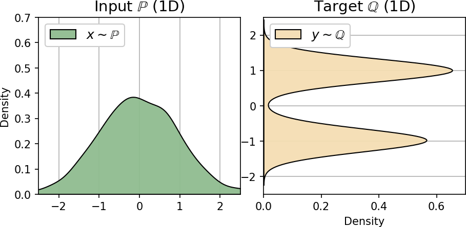
(a) Input and output distributions.

(b) Learned plan $\hat{\pi}$ and marginal $\hat{T}_{\#}(\mathbb{P}\times\mathbb{S})$, test 1.

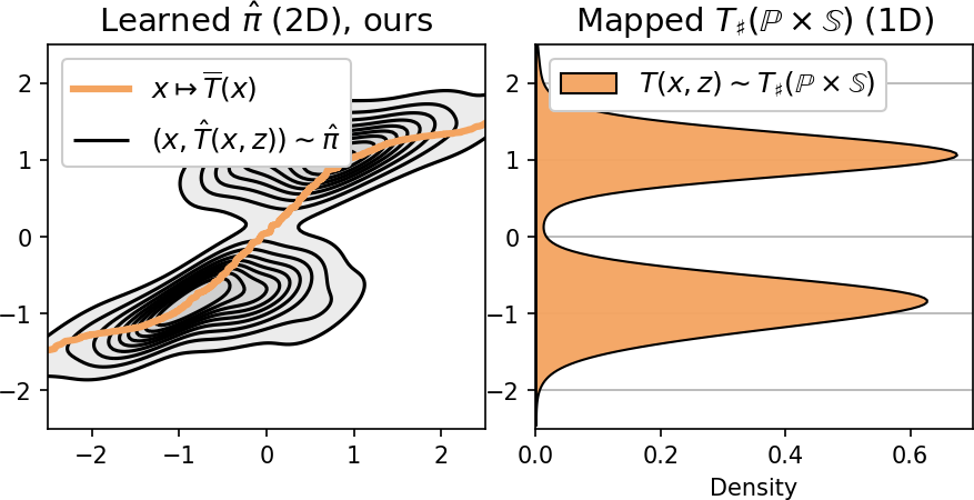
(c) Learned plan $\hat{\pi}$ and marginal $\hat{T}_{\#}(\mathbb{P}\times\mathbb{S})$, test 2.

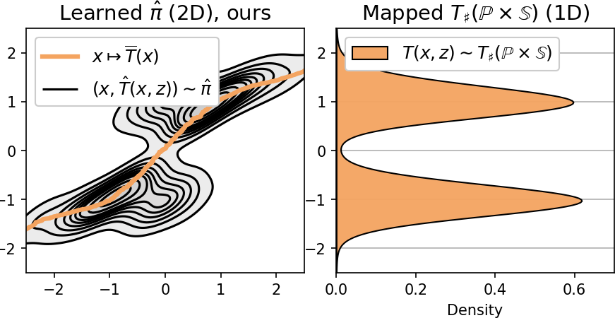
(d) Learned plan $\hat{\pi}$ and marginal $\hat{T}_{\#}(\mathbb{P}\times\mathbb{S})$, test 3.

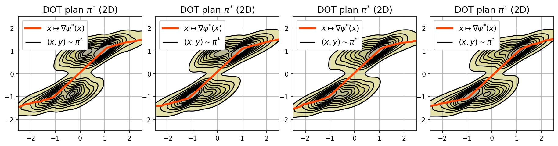
(e) Various optimal plans $\pi^{*}$ learned by discrete OT (considered here as the ground truth).

Figure 10: Stochastic plans between toy 1D distributions (Figure 10(a)) learned by NOT (Figures 10(b), 10(c), 10(d)) and discrete OT (Figure 10(e)) with the 1-weak quadratic cost. The figures with the 2D transport plans also demonstrate the average map $x\mapsto\int_{\mathcal{Y}}yd\hat{\pi}(y|x)$ (conditional expectation).

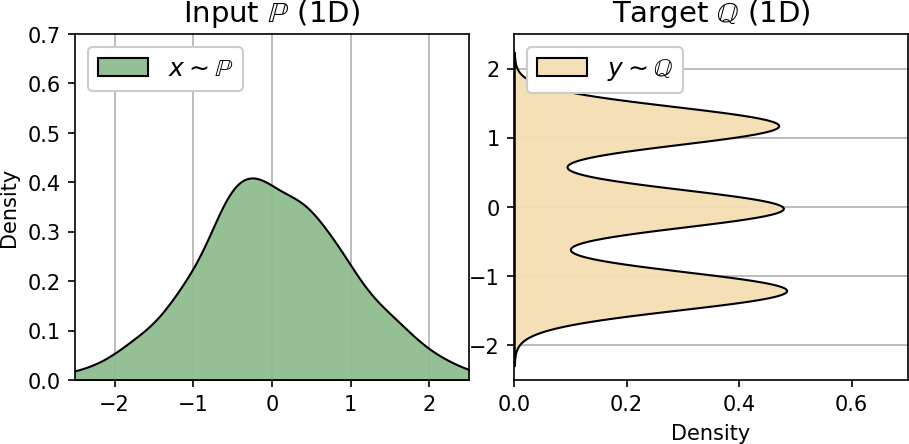
(a) Input and output distributions.

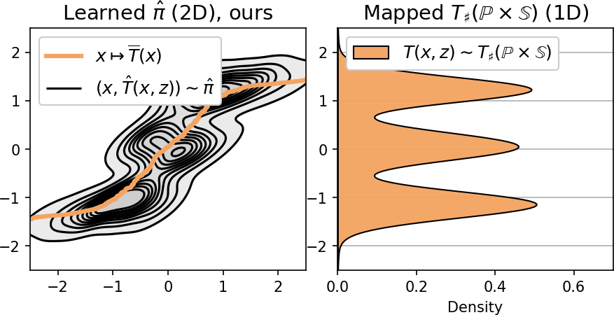
(b) Learned plan $\hat{\pi}$ and marginal $\hat{T}_{\#}(\mathbb{P}\times\mathbb{S})$, test 1.

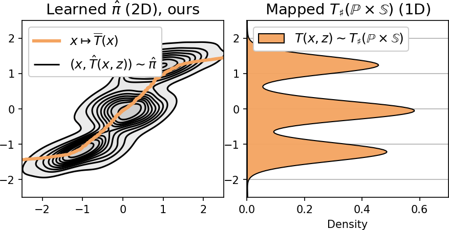
(c) Learned plan $\hat{\pi}$ and marginal $\hat{T}_{\#}(\mathbb{P}\times\mathbb{S})$, test 2.

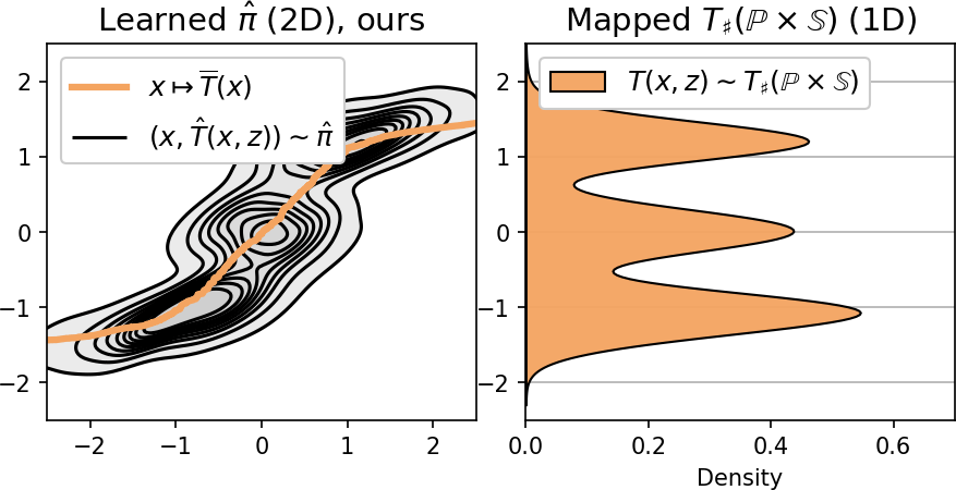
(d) Learned plan $\hat{\pi}$ and marginal $\hat{T}_{\#}(\mathbb{P}\times\mathbb{S})$, test 3.

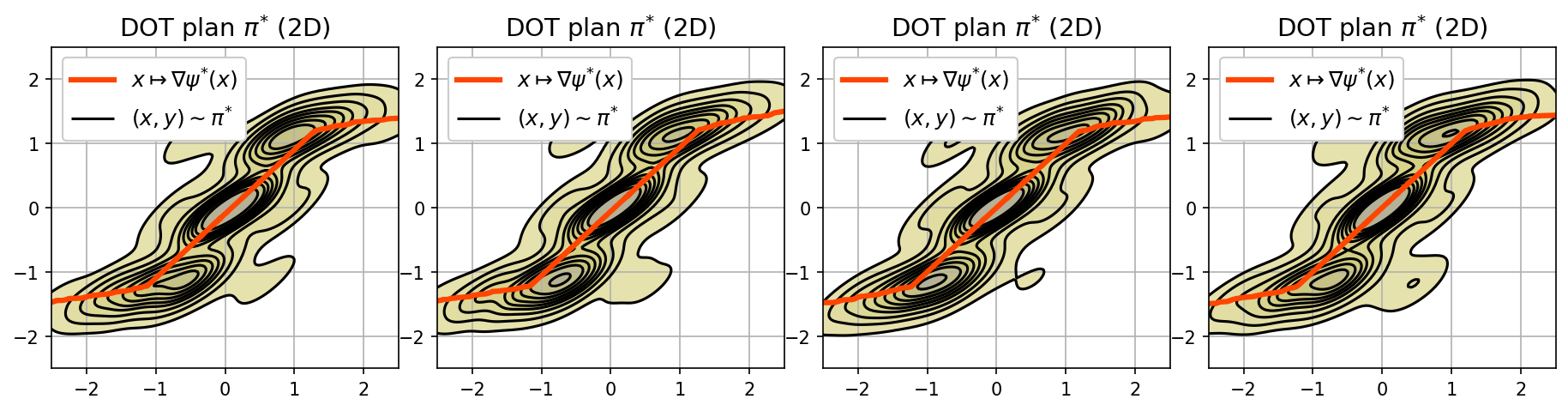
(e) Various optimal plans $\pi^{*}$ learned by discrete OT (considered here as the ground truth).

Figure 11: Stochastic plans between toy 1D distributions (Figure 11(a)) learned by NOT (Figures 11(b), 11(c), 11(d)) and discrete OT (Figure 11(e)) with the 1-weak quadratic cost. The figures with the 2D transport plans also demonstrate the average map $x\mapsto\int_{\mathcal{Y}}yd\hat{\pi}(y|x)$ (conditional expectation).

Appendix D Comparison with Principal Unpaired Translation Methods

We compare our Algorithm 1 with popular models for unpaired translation. We consider handbags $\rightarrow$ shoes ($64\times 64$), celeba male $\rightarrow$ female ($64\times 64$), outdoor $\rightarrow$ church ($128\times 128$) translation. For quantitative comparison, we compute Frechet Inception Distance (Heusel et al., 2017, FID) of the mapped test handbags subset w.r.t. the test shoes subset. The scores of our method and alternatives are given in Table 1. The translated images are shown in Figures 12, 13, 14.

Methods. We compare our method with one-to-one CycleGAN (Zhu et al., 2017a), DiscoGAN (Kim et al., 2017) and with one-to-many AugCycleGAN (Almahairi et al., 2018) and MUNIT (Huang et al., 2018). We use the official or community implementations with the hyperparameters from the respective papers. We choose the above-mentioned methods for comparison because they are principal methods for one-to-one and one-to-many translation. Recent methods (GMM-UNIT (Liu et al., 2020), COCO-FUNIT (Saito et al., 2020), StarGAN (Choi et al., 2020)) are based on them and focus on specific details/setups such as style/content separation, few-shot learning, disentanglement, multi-domain transfer, which are out of scope of our paper.

Discussion. Existing one-to-one methods visually preserve the style during translation comparably to our method. Alternative one-to-many methods do not preserve the style at all. When the input and output domains are similar (handbags$\rightarrow$shoes, celeba male $\rightarrow$ female), the FID scores of all the models are comparable. However, most models are outperformed by NOT when the domains are distant (outdoor $\rightarrow$ church), see Figure 14 and the last row in Table 1. For completeness, in Table 2 we compare the number of hyperparameters of the translation methods in view. Note that in contrast to the other methods, we optimize only $2$ neural networks – transport map and potential.

Type	One-to-one			One-to-many
Method	Disco GAN	Cycle GAN	NOT (ours)	AugCycle GAN	MUNIT	NOT (ours)
Handbags $\rightarrow$ shoes (64$\times$ 64)	22.42	16.00	13.77	18.84 $\pm$ 0.11	15.76 $\pm$ 0.11	13.44 $\pm$ 0.12
Celeba male $\rightarrow$ female (64$\times$ 64)	35.64	17.74	13.23	12.94 $\pm$0.08	17.07 $\pm$0.11	11.96 $\pm$0.07
Outdoor $\rightarrow$ church (128$\times$ 128)	75.36	46.39	25.5	51.42 $\pm$0.12	31.42 $\pm$0.16	25.97 $\pm$0.14

Table 1: Test FID$\downarrow$ of the considered unpaired translation methods.

Type	One-to-one			One-to-many
Method	Disco GAN	Cycle GAN	NOT (ours)	AugCycle GAN	MUNIT	NOT (ours)
Hyperparameters of optimization objectives	None	Weights of cycle and identity losses $\lambda_{cyc},\lambda_{id}$	None	Weights of cycle losses $\gamma_{1},\gamma_{2}$	Weights of reconstruction losses $\lambda_{x},\lambda_{c},\lambda_{s}$	Diversity control parameter $\gamma$
Total number of hyperparameters	0	2	0	2	3	1
Networks	2 generators, 2$\times$29.2M 2 discriminators 2$\times$0.7M	2 generators 2$\times$11.4M 2 discriminators 2$\times$2.8M	1 transport 9.7M, 1 potential 22.9M [32.4M∗]	2 generators 2$\times$1.1M, 2 discriminators 2$\times$2.8M, 2 encoders 2$\times$1.4M	2 generators 2$\times$15.0M, 2 discriminators 2$\times$8.3M	1 transport map 9.7M, 1 potential 22.9M [32.4M∗]
Total number of networks and parameters	4 networks 59.8M	4 networks 28.2M	2 networks 32.6M [42.1M∗]	6 networks 7.0M	4 networks 46.6M	2 networks 32.6M [42.1M∗]

Table 2: Comparison of the number of hyperparameters of the optimization objectives, the number of networks and their parameters for the considered unpaired translation methods for 64$\times$64 images.

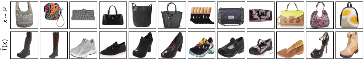
(a) NOT (ours, $\mathbb{W}_{2}$), one-to-one.

(b) DiscoGAN, one-to-one.

(c) CycleGAN, one-to-one.

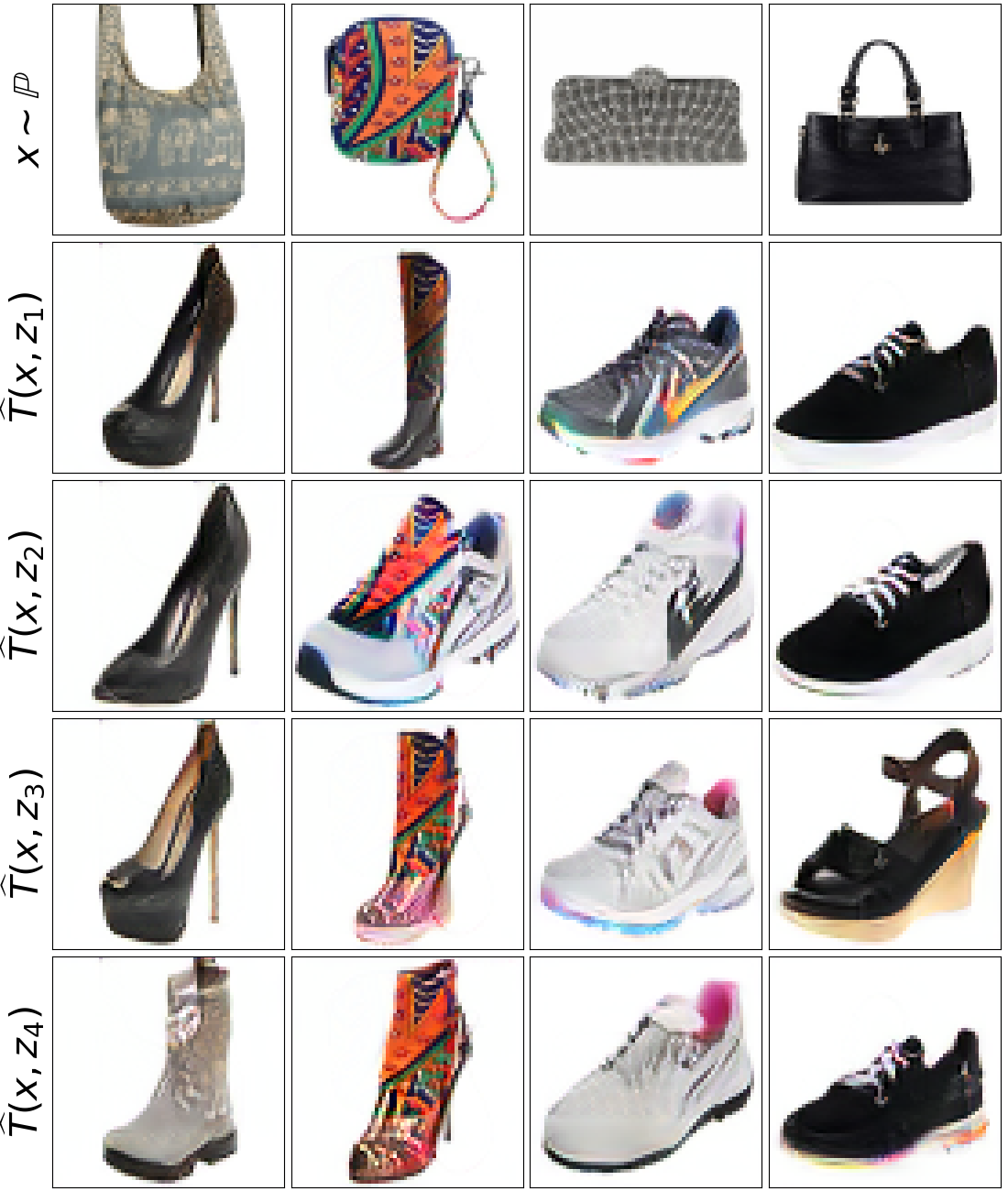
(d) NOT (ours, $\mathcal{W}_{2,\frac{2}{3}}$), one-to-many.

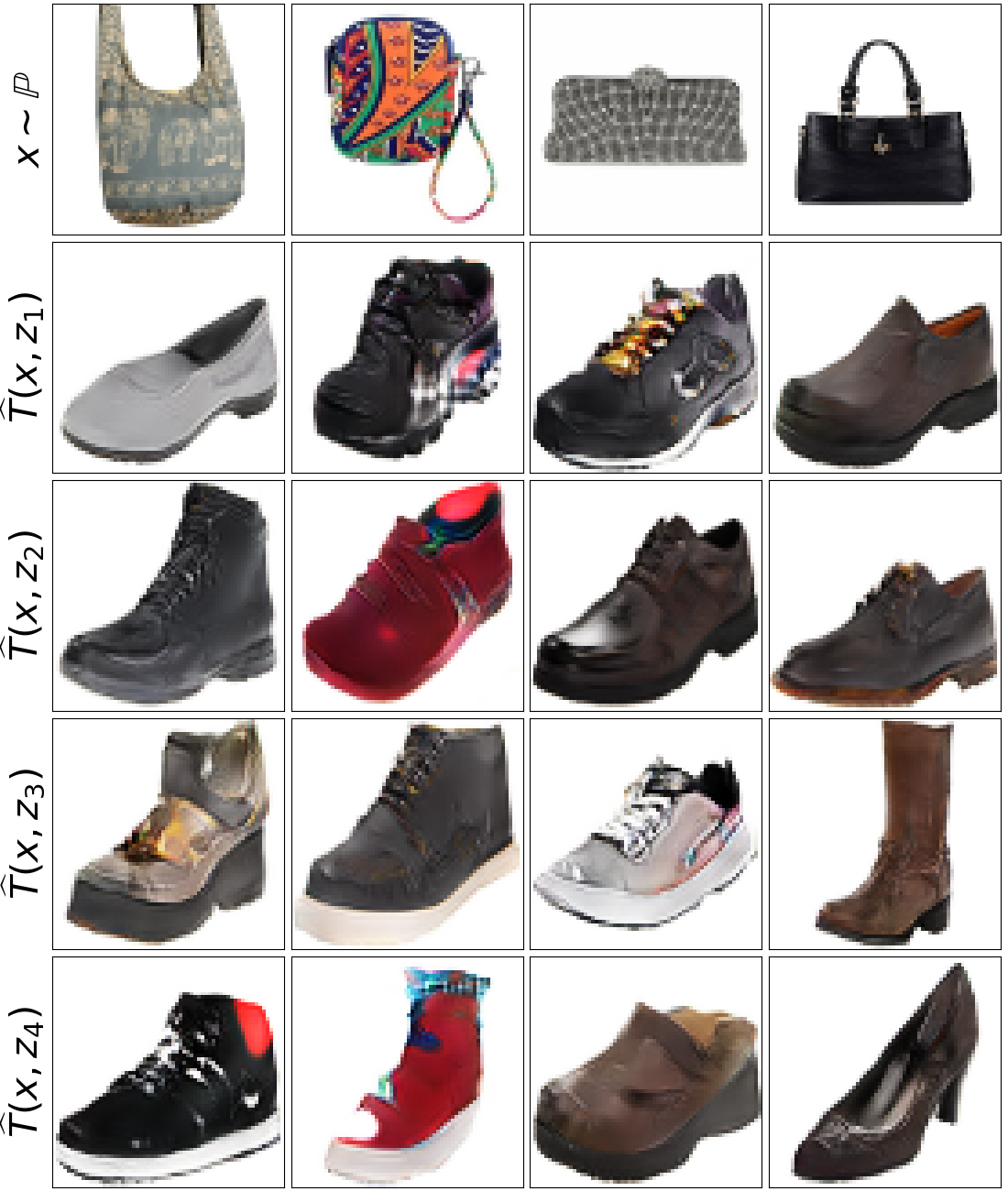
(e) MUNIT, one-to-many.

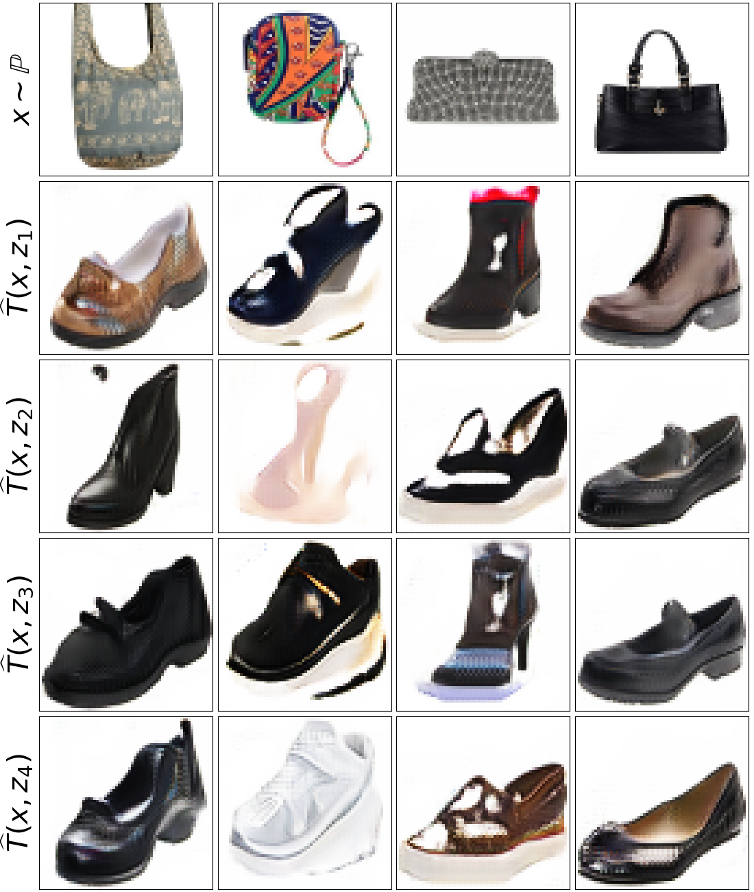
(f) AugCycleGAN

Figure 12: Handbags $\rightarrow$ shoes translation ($64\times 64$) by the methods in view.

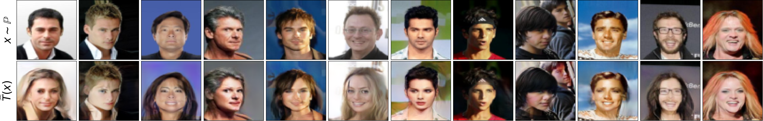
(a) NOT (ours, $\mathbb{W}_{2}$), one-to-one.

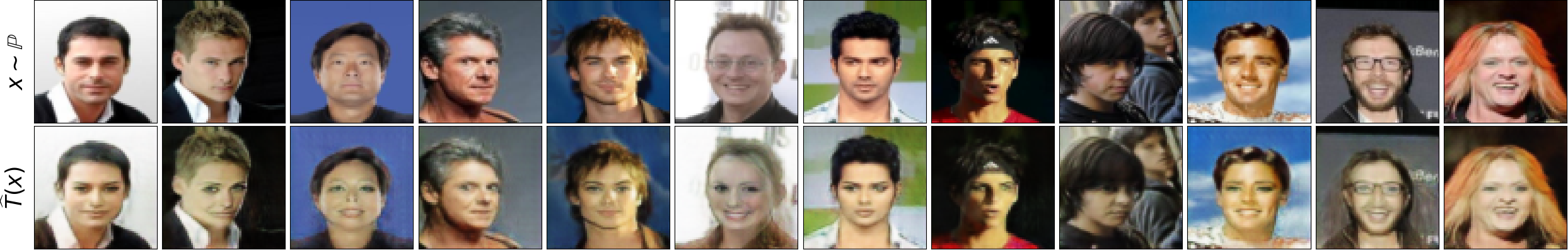
(b) DiscoGAN, one-to-one.

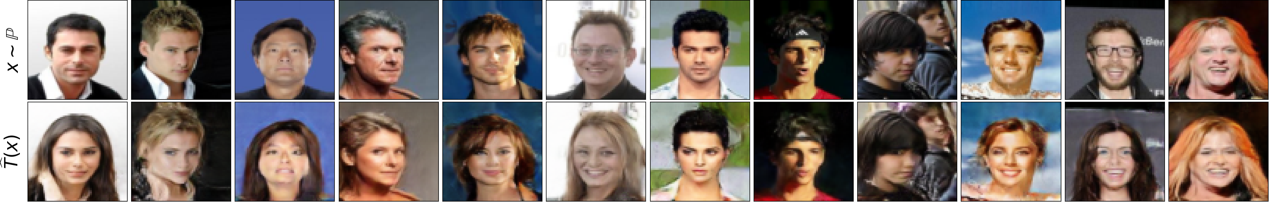
(c) CycleGAN, one-to-one.

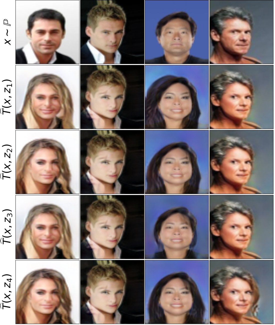
(d) NOT (ours, $\mathcal{W}_{2,\frac{2}{3}}$), one-to-many.

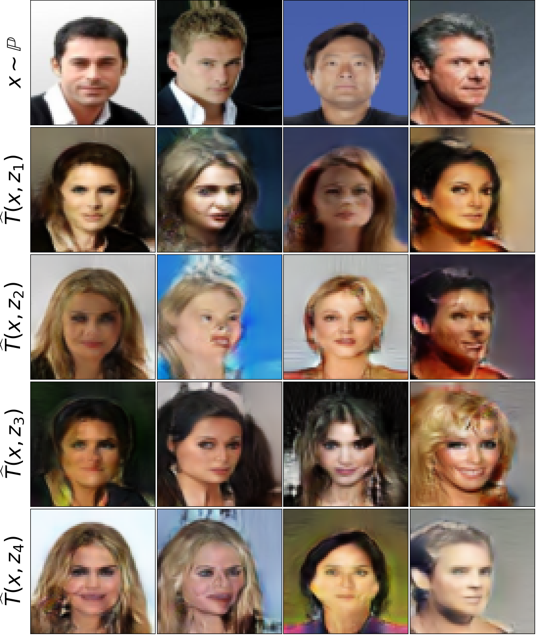
(e) MUNIT, one-to-many.

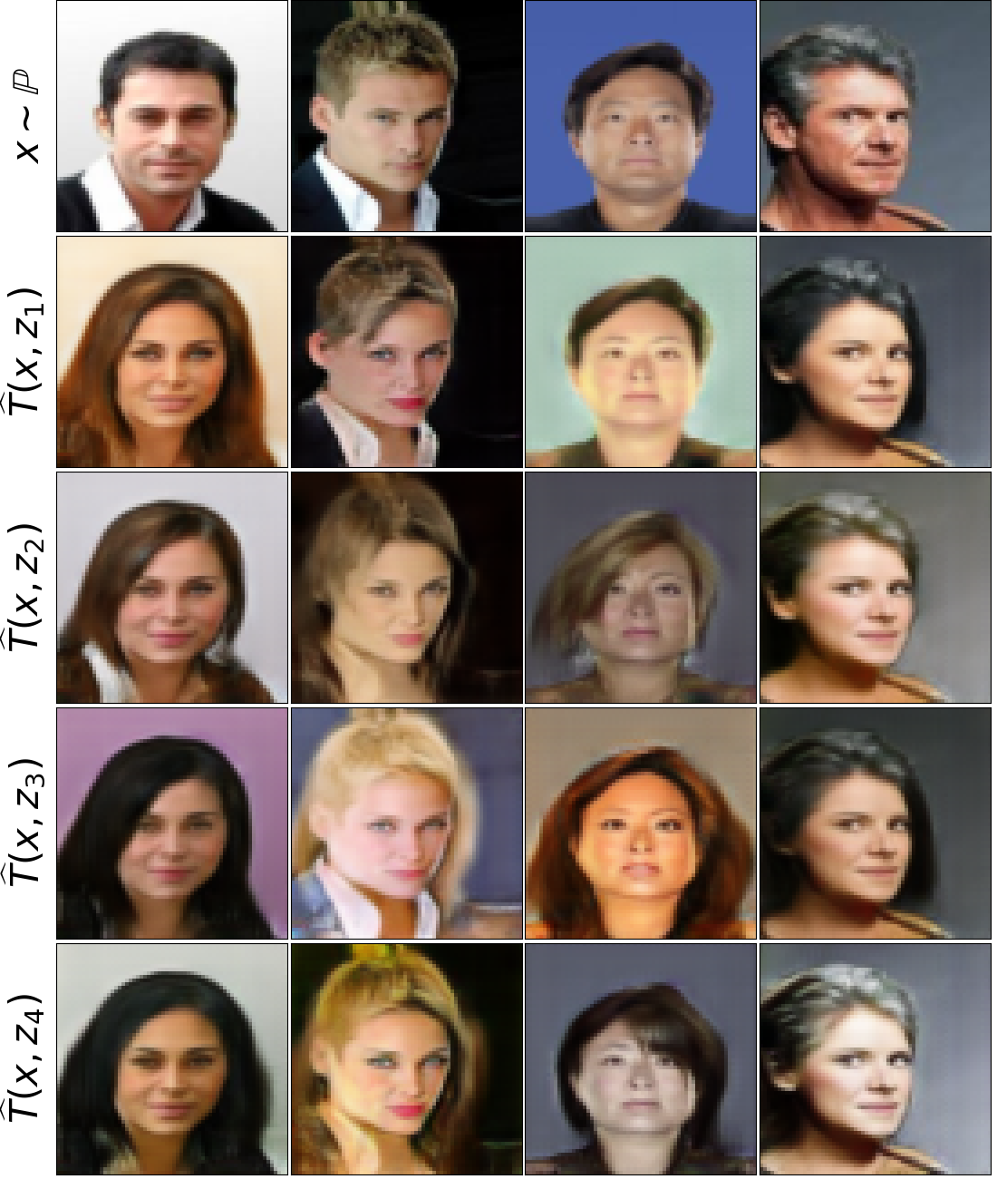
(f) AugCycleGAN

Figure 13: Celeba (male) $\rightarrow$ Celeba (female) translation ($64\times 64$) by the methods in view.

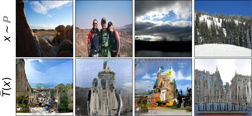
(a) DiscoGAN, one-to-one.

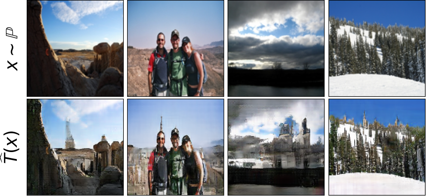
(b) CycleGAN, one-to-one.

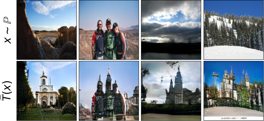
(c) NOT (ours, $\mathbb{W}_{2}$), one-to-one.

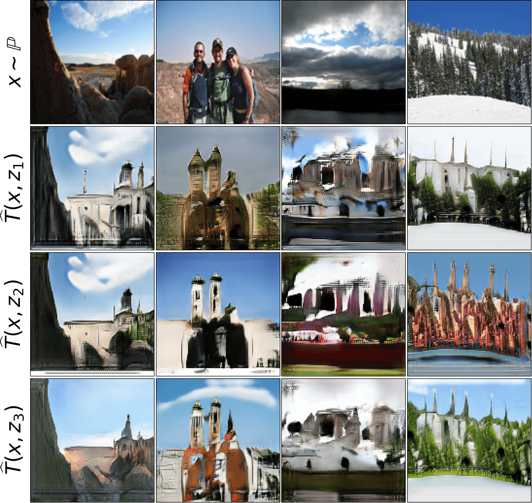
(d) AugCycleGAN, one-to-many.

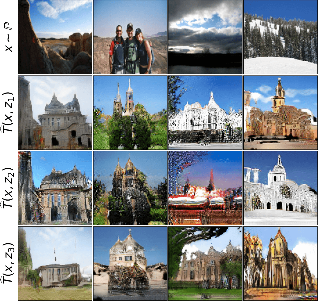
(e) MUNIT, one-to-many.

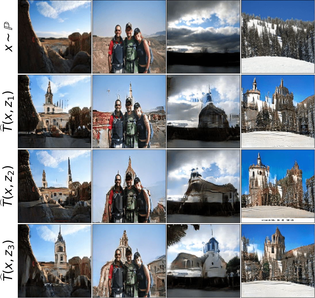
(f) NOT (ours, $\mathcal{W}_{2,\frac{2}{3}}$), one-to-many.

Figure 14: Outdoor $\rightarrow$ church ($128\times 128$) translation with various methods.

Appendix E Experimental Details

Pre-processing. We beforehand rescale anime face images to $512\times 512$, and do $256\times 256$ crop with the center located $14$ pixels above the image center to get the face. Next, for all these datasets, we rescale RGB channels to $[-1,1]$ and resize images to the required size ($64\times 64$ or $128\times 128$). We do not apply any augmentations to data.

Neural networks. We use WGAN-QC discriminator’s ResNet architecture (Liu et al., 2019) for potential $f$. We use UNet (Ronneberger et al., 2015) as the stochastic transport map $T(x,z)$. The noise $z$ is simply an additional $4$th input channel (RGBZ), i.e., the dimension of the noise equals the image size ($64\times 64$ or $128\times 128$). We use high-dimensional Gaussian noise with axis-wise $\sigma=0.1$.

Optimization. We use the Adam optimizer (Kingma & Ba, 2014) with the default betas for both $T_{\theta}$ and $f_{\omega}$. The learning rate is $lr=1\cdot 10^{-4}$. The batch size is $|X|=64$. The number of inner iterations is $k_{T}=10$. When training with the weak cost (4), we sample $|Z_{x}|=4$ noise samples per each image $x$ in batch. In toy experiments, we do $10$K total iterations of $f_{\omega}$ update. In the experiments with unpaired translation, our Algorithm 1 converges in $\approx 40$K iterations for most datasets.

Dynamic weak cost. In 5.3, we train the algorithm with the gradually changing $\gamma$. Starting from $\gamma=0$, we linearly increase it to the desired value ($\frac{2}{3}$ or $1$) during 25K first iterations of $f_{\omega}$.

Stability of training. In several cases, we noted that the optimization fluctuates around the saddle points or diverges. An analogous behavior of saddle point methods for OT has been observed in (Korotin et al., 2021b). For the $\gamma$-weak quadratic cost ($\gamma>0$), we sometimes experienced instabilities when the input $\mathbb{P}$ is notably less disperse than $\mathbb{Q}$ or when the parameter $\gamma$ is high. Studying this behaviour and improving stability/convergence of the optimization is a promising research direction.

Computational complexity. The time and memory complexity of training deterministic OT maps $T(x)$ is comparable to that of training usual generative models for unpaired translation. Our networks converge in 1-3 days on a Tesla V100 GPU (16 GB); wall-clock times depend on the datasets and the image sizes. Training stochastic $T(x,z)$ is harder since we sample multiple random $z$ per $x$ (we use $|Z|=4$). Thus, we learn stochastic maps on 4 $\times$ Tesla V100 GPUs.

Appendix F Optimality of Solutions for Strictly Convex Costs

Our Lemma 16 proves that optimal maps $T^{*}$ are contained in the $\operatorname*{arg\,inf}_{T}$ sets of optimal potentials $f^{*}$ but leaves the question what else may be contained in these $\operatorname*{arg\,inf}_{T}$ sets open. Our following result shows that for strictly convex costs, nothing else beside OT maps is contained there.

Lemma 5 (Solutions of the maximin problem are OT maps).

Let $C(x,\mu)$ be a weak cost which is strictly convex in $\mu$. Assume that there exists at least one potential $f^{*}$ which maximizes dual form (5). Consider any such optimal potential $f^{*}\in\operatorname*{arg\,sup}_{f}\inf_{T}\mathcal{L}(f,T)$. It holds that

$$\hat{T}\in\operatorname*{arg\,inf}_{T}\mathcal{L}(f^{*},T)\Rightarrow\hat{T}\mbox{ is a stochastic OT map}.$$

Proof of Lemma (5)..

By the definition of $f^{*}$, we have

$$\mathcal{L}(f^{*},\hat{T})=\sup_{f}\inf_{T}\mathcal{L}(f,T)=\mbox{Cost}(\mathbb{P},\mathbb{Q}),$$

i.e., $\hat{T}$ attains the optimal cost. It remains to check that it satisfies $\hat{T}\sharp(\mathbb{P}\times\mathbb{S})=\mathbb{Q}$, i.e., $\hat{T}$ generates $\mathbb{Q}$ from $\mathbb{P}$. Let $T^{*}$ be any true stochastic OT map. We denote $\mu_{x}^{*}=T^{*}(x,\cdot)\sharp\mathbb{S}$ and $\hat{\mu}_{x}=\hat{T}(x,\cdot)\sharp\mathbb{S}$ for all $x\in\mathcal{X}$ and define $\mu^{1}_{x}=\frac{1}{2}(\mu^{*}_{x}+\hat{\mu}_{x})$. Let $T^{1}:\mathcal{X}\times\mathcal{Z}\rightarrow\mathcal{Y}$ be any stochastic map which satisfies $T^{1}(x,\cdot)\sharp\mathbb{S}=\mu_{x}^{1}$ for all $x\in\mathcal{X}$ (4.1). By using the change of variables, we derive

$$\mbox{Cost}(\mathbb{P},\mathbb{Q})\geq\mathcal{L}(f^{*},T^{1})=\int_{\mathcal{X}}C(x,\mu_{x}^{1})d\mathbb{P}(x)-\int_{\mathcal{X}}\big{[}\int_{\mathcal{Y}}f^{*}(y)d\mu_{x}^{1}(y)\big{]}d\mathbb{P}(x)+\int_{\mathcal{Y}}f^{*}(y)\mathbb{Q}(y).$$ (23)

Since $C$ is convex in the second argument, we have

$$C(x,\mu_{1}^{x})=C\big{(}x,\frac{1}{2}(\mu^{*}_{x}+\hat{\mu}_{x})\big{)}\geq\frac{1}{2}C(x,\mu^{*}_{x})+\frac{1}{2}C(x,\hat{\mu}_{x}).$$ (24)

Since $C$ is strictly convex, the equality in (24) is possible only when $\mu_{x}^{*}=\hat{\mu}_{x}$. We also note that

$$\int_{\mathcal{Y}}f^{*}(y)d\mu_{x}^{1}(y)=\int_{\mathcal{Y}}f^{*}(y)d\frac{(\mu^{*}_{x}+\hat{\mu}_{x})}{2}(y)=\frac{1}{2}\int_{\mathcal{Y}}f^{*}(y)d\mu^{*}_{x}(y)+\frac{1}{2}\int_{\mathcal{Y}}f^{*}(y)d\hat{\mu}_{x}(y).$$

We substitute these findings to $\mathcal{L}(f^{*},T^{1})$ and get

$$\mbox{Cost}(\mathbb{P},\mathbb{Q})\geq\mathcal{L}(f^{*},T^{1})\geq\frac{1}{2}\mathcal{L}(f^{*},T^{*})+\frac{1}{2}\mathcal{L}(f^{*},\hat{T})=\\ \frac{1}{2}\mbox{Cost}(\mathbb{P},\mathbb{Q})+\frac{1}{2}\mbox{Cost}(\mathbb{P},\mathbb{Q})=\mbox{Cost}(\mathbb{P},\mathbb{Q}).$$

Thus, (23) is an equality $\mathbb{P}$-almost surely for all $x\in\mathcal{X}$ and $\mu_{x}^{*}=\hat{\mu}_{x}$ holds $\mathbb{P}$-almost surely. This means that $T^{*}$ and $\hat{T}$ generate the same distribution from $\mathbb{P}\times\mathbb{S}$, i.e., $\hat{T}$ is a stochastic OT map. ∎

Our generic framework allows learning stochastic transport maps (Lemma 16). For strictly convex costs, all the solutions of our objective (14) are guaranteed to be stochastic OT maps (Lemma 5). In the experiments, we focus on strong and weak quadratic costs, which are not strictly convex but still provide promising performance in the downstream task of unpaired image-to-image translation (5). Developing strictly convex costs is a promising research avenue for the future work.

Appendix G Relation to Prior Works in Unbalanced Optimal Transport

In the context of OT, (Yang & Uhler, 2019) employ a stochastic generator to learn a transport plan $\pi$ in the unbalanced OT problem (Chizat, 2017). Due to this, their optimization objective slightly resembles our objective (15). However, this similarity is deceptive. Unlike strong (2) or weak (3) OT, the unbalanced OT is an unconstrained problem, i.e., there is no need to satisfy $\pi\in\Pi(\mathbb{P},\mathbb{Q})$. This makes unbalanced OT easier to handle: to optimize it one just has to parametrize the plan $\pi$ and backprop through the loss. The challenging part with which the authors deal is the estimation of the $\phi$-divergence terms in the unbalanced OT objective. These terms can be interpreted as a soft relaxation of the constraints $\pi\in\Pi(\mathbb{P},\mathbb{Q})$, i.e., penalization for disobeying the constraints. The authors compute these terms by employing the variational (dual) formula from $f$-GAN (Nowozin et al., 2016). This yields a GAN-style optimization problem $\min_{T}\max_{f}$ which is similar to other problems in the generative adversarial framework. The problem we tackle is strong (2) and weak (3) OT which requires enforcing of the constraint $\pi\in\Pi(\mathbb{P},\mathbb{Q})$. We reformulate the dual (weak) OT problem (5) into maximin problem (15) which can be used to recover the OT plan (via the stochastic map $T$). Our approach can be viewed as a hard enforcement of the constraints. Our $\max_{f}\min_{T}$ saddle point problem (15) is atypical for the traditional generative adversarial framework.

Appendix H Additional Experimental Results

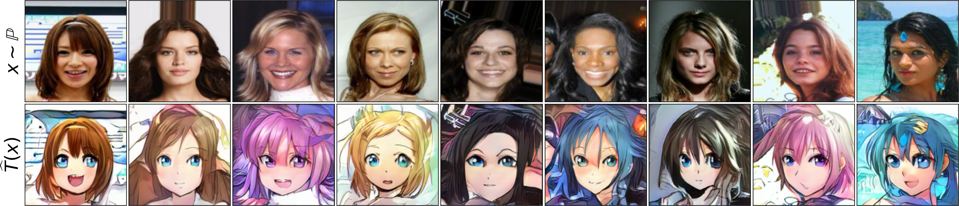
(a) Celeba (female) $\rightarrow$ anime translation, $128\times 128$.

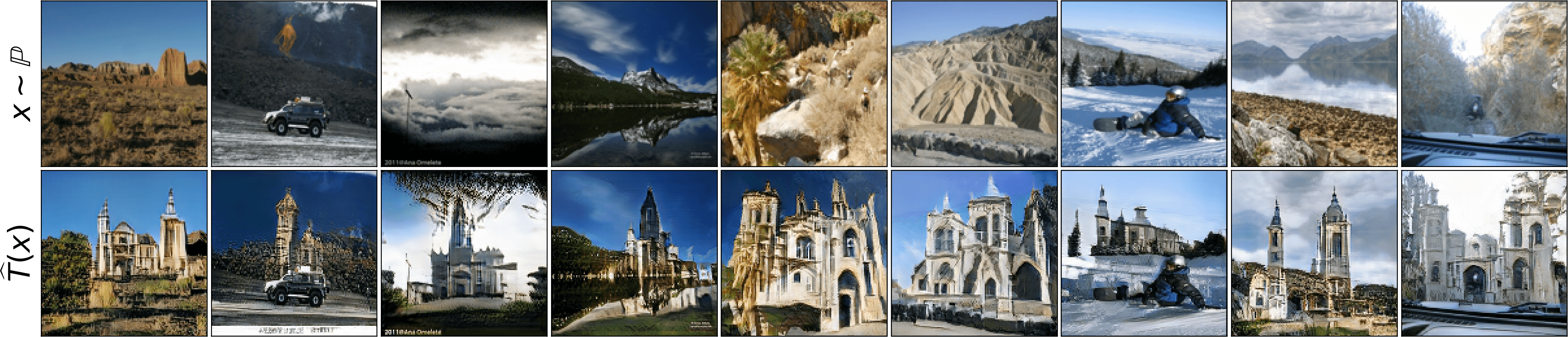
(b) Outdoor $\rightarrow$ church, $128\times 128$.

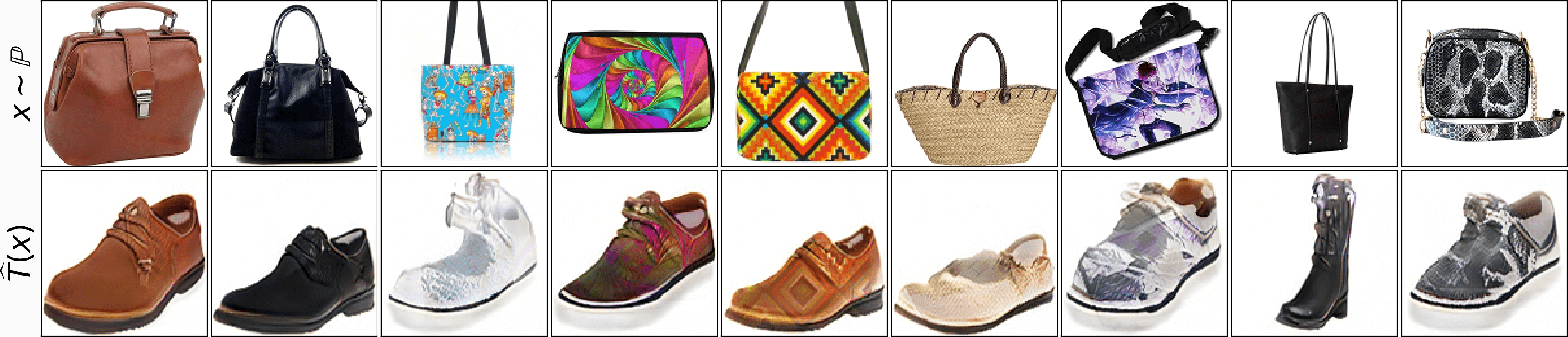
(c) Handbags $\rightarrow$ shoes, $128\times 128$.

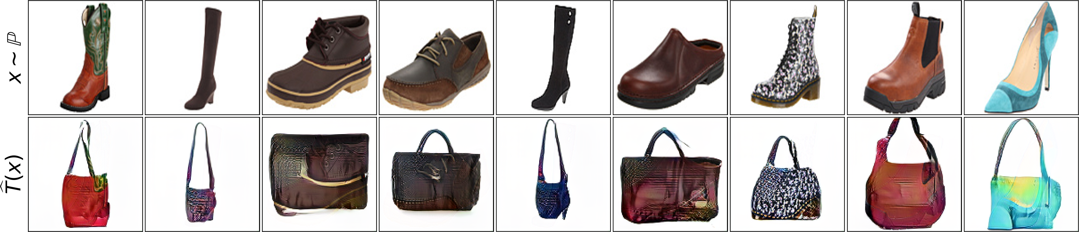
(d) Shoes $\rightarrow$ handbags, $128\times 128$.

Figure 15: Unpaired translation with OT maps ($\mathbb{W}_{2}$). Additional examples (part 1).

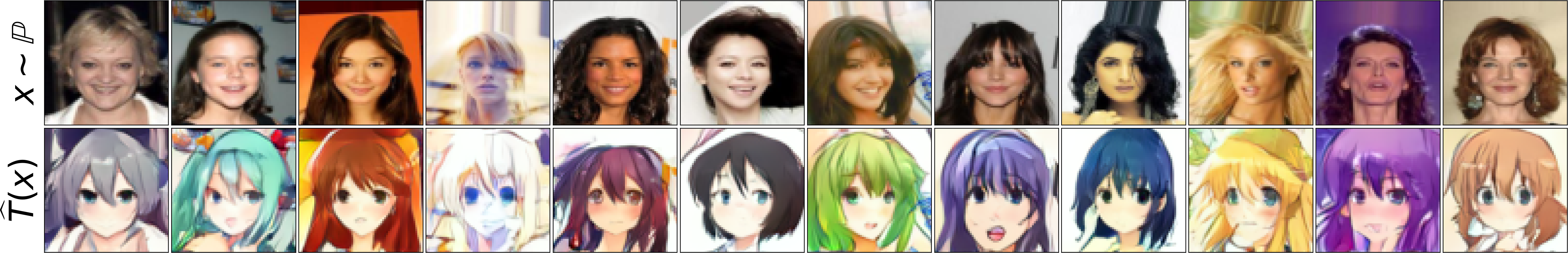
(a) Celeba (female) $\rightarrow$ anime translation, $64\times 64$.

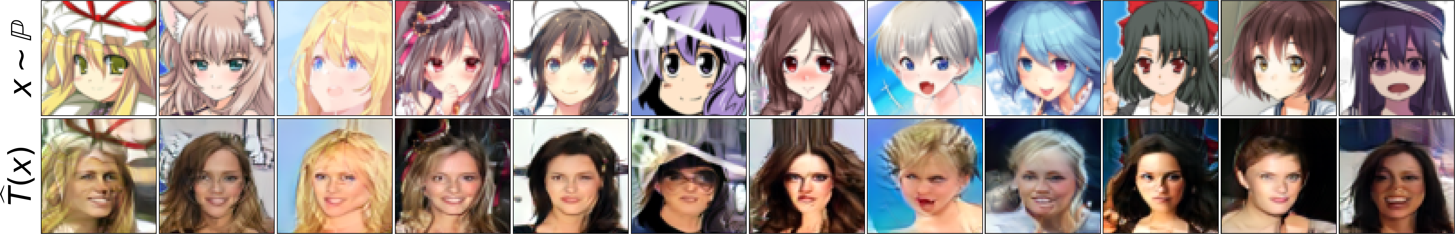
(b) Anime $\rightarrow$ celeba (female) translation, $64\times 64$.

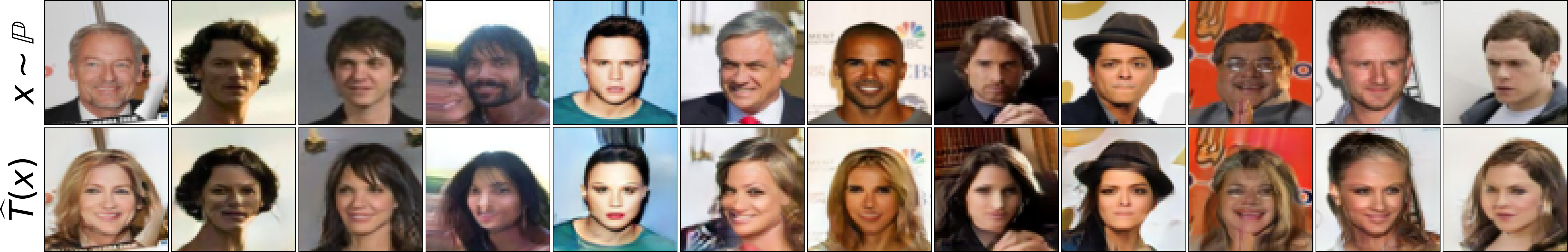
(c) Celeba (male) $\rightarrow$ celeba (female) translation, $64\times 64$.

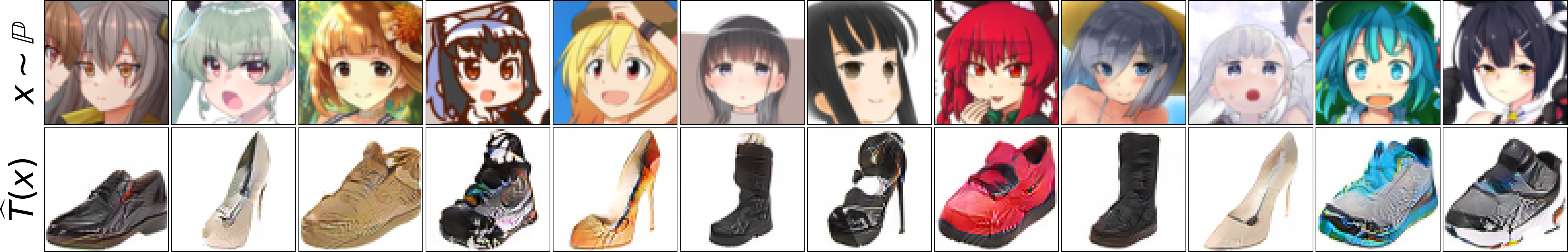
(d) Anime $\rightarrow$ shoes translation, $64\times 64$.

Figure 16: Unpaired translation with OT maps ($\mathbb{W}_{2}$). Additional examples (part 2).

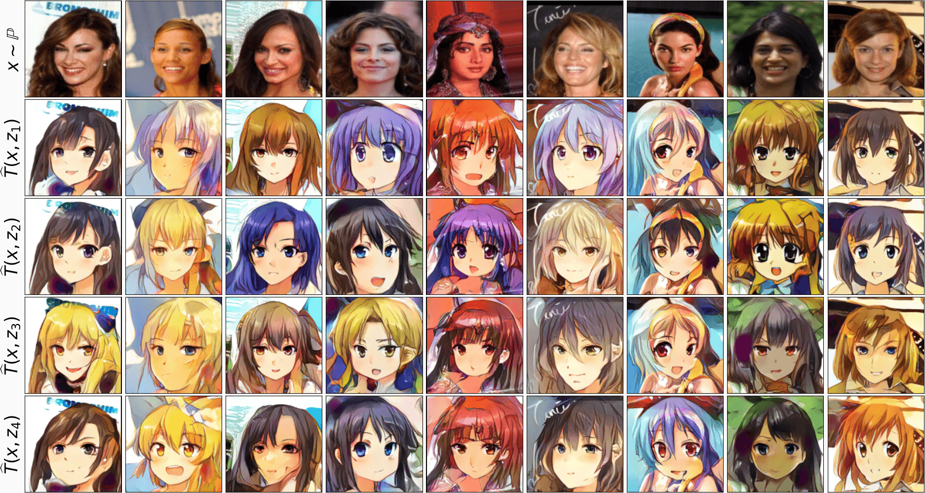
(a) Input images $x$ and random translated examples $T(x,z)$.

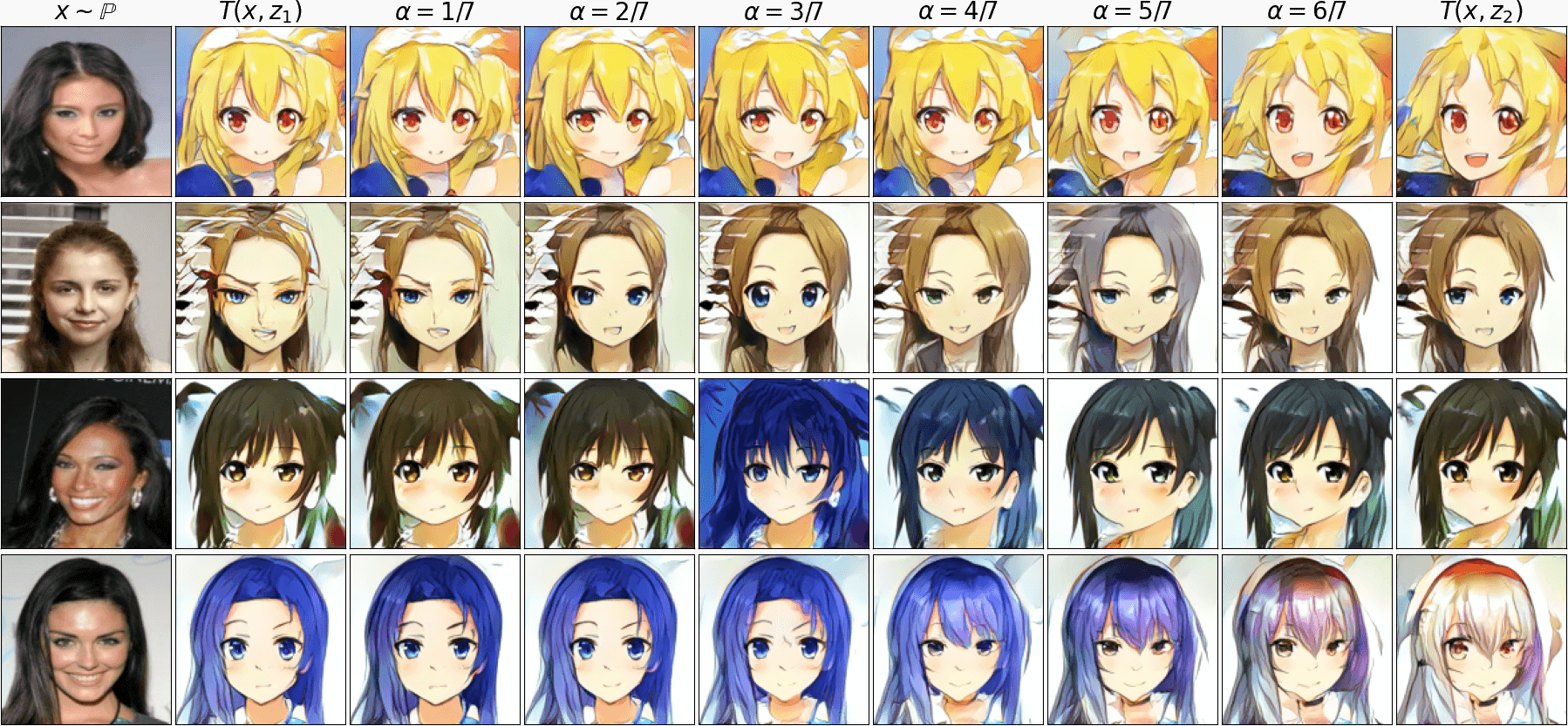
(b) Interpolation in the conditional latent space, $z=(1-\alpha)z_{1}+\alpha z_{2}$.

Figure 17: Celeba (female) $\rightarrow$ anime, $128\times 128$, stochastic. Additional examples.

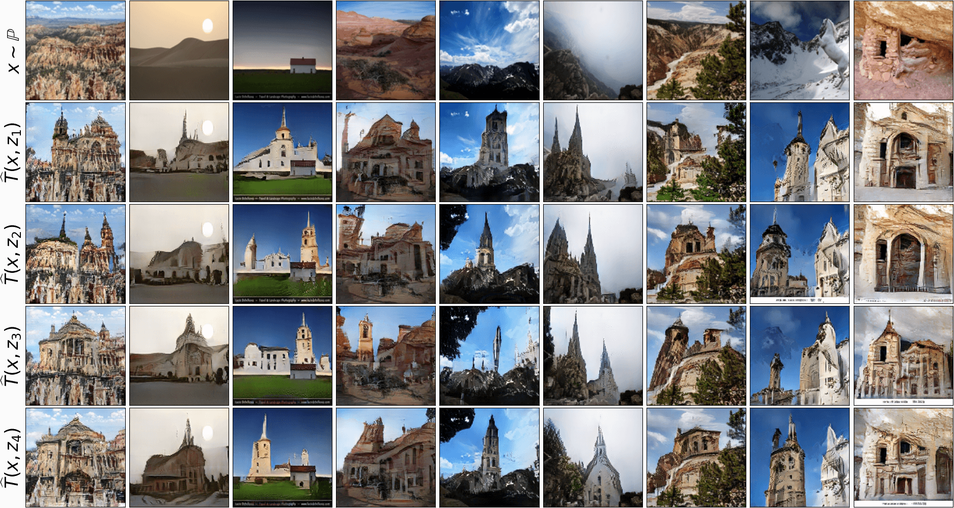
(a) Input images $x$ and random translated examples $T(x,z)$.

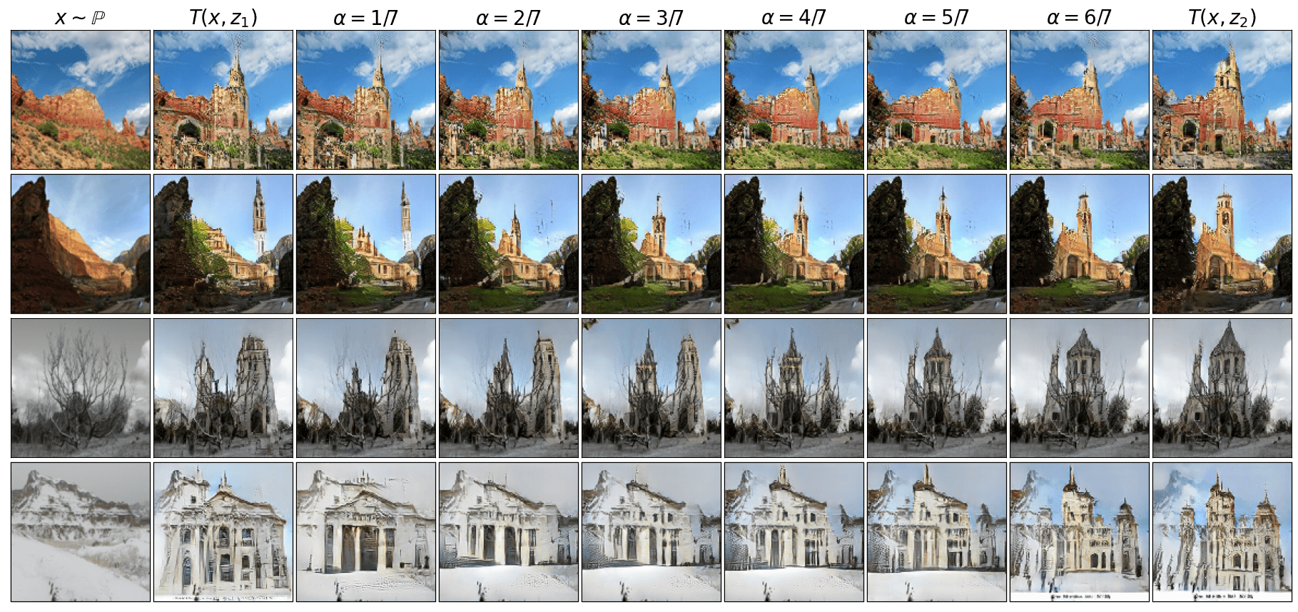
(b) Interpolation in the conditional latent space, $z=(1-\alpha)z_{1}+\alpha z_{2}$.

Figure 18: Outdoor $\rightarrow$ church, $128\times 128$, stochastic. Additional examples.

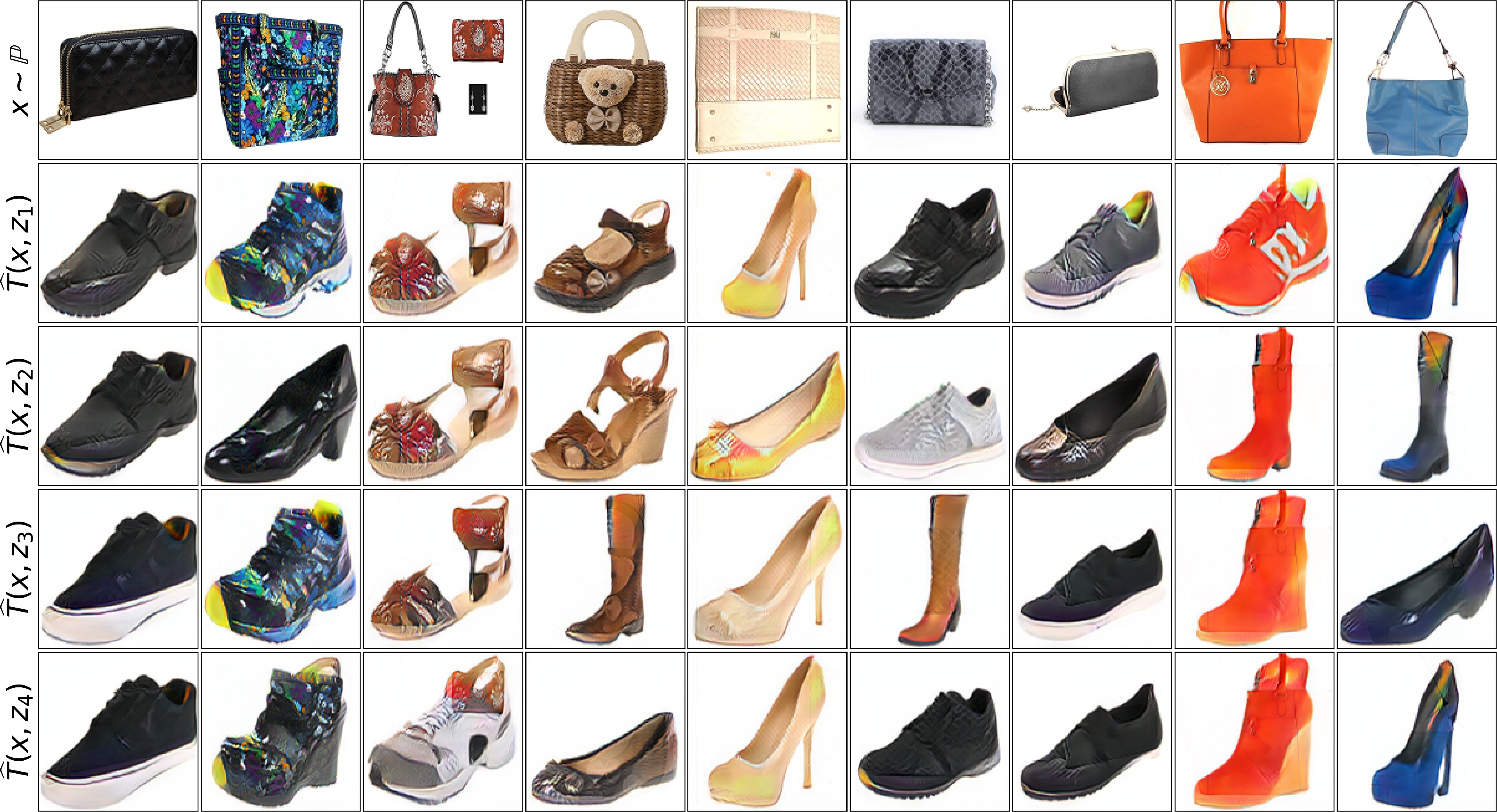
(a) Input images $x$ and random translated examples $T(x,z)$.

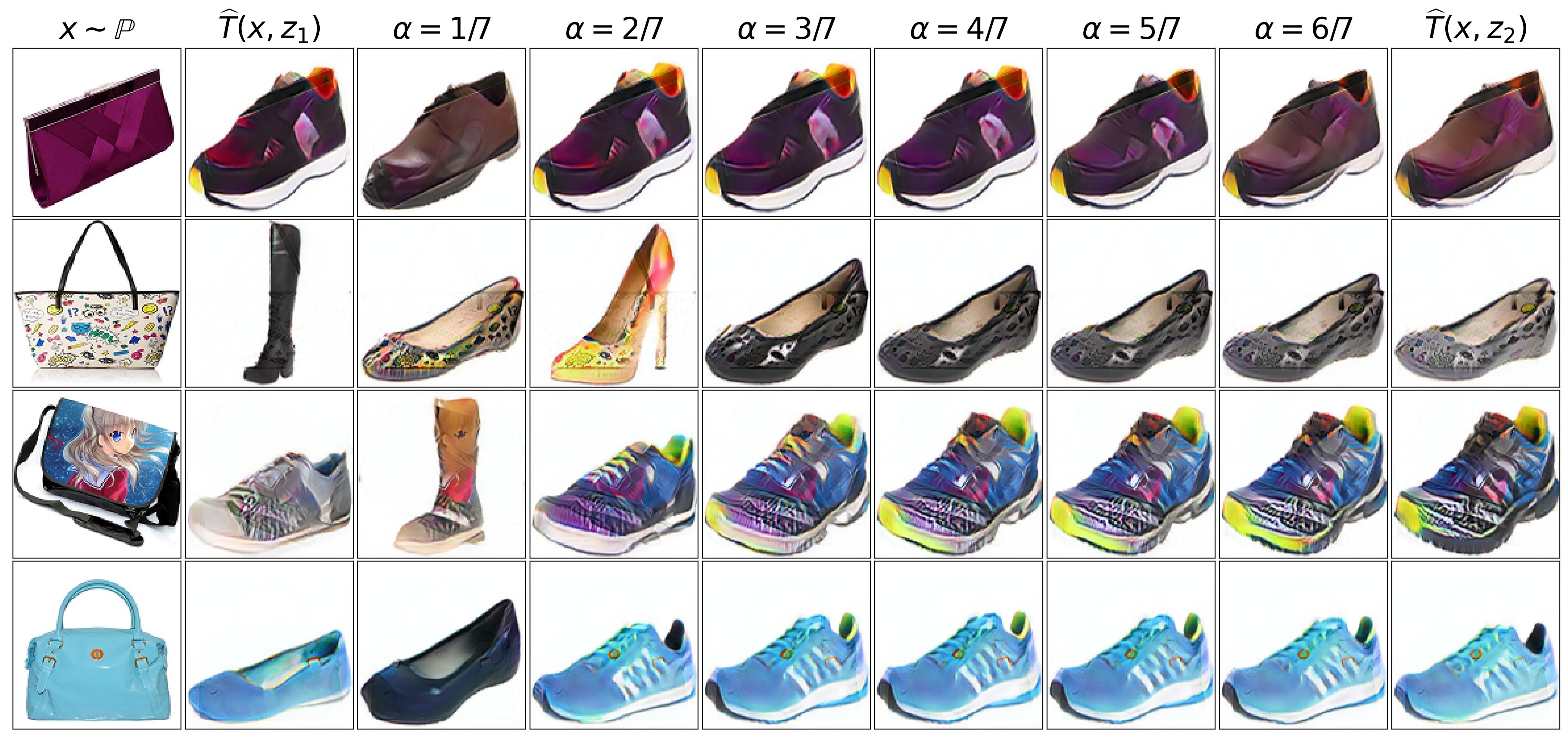
(b) Interpolation in the conditional latent space, $z=(1-\alpha)z_{1}+\alpha z_{2}$.

Figure 19: Handbags $\rightarrow$ shoes translation, $128\times 128$, stochastic. Additional examples.

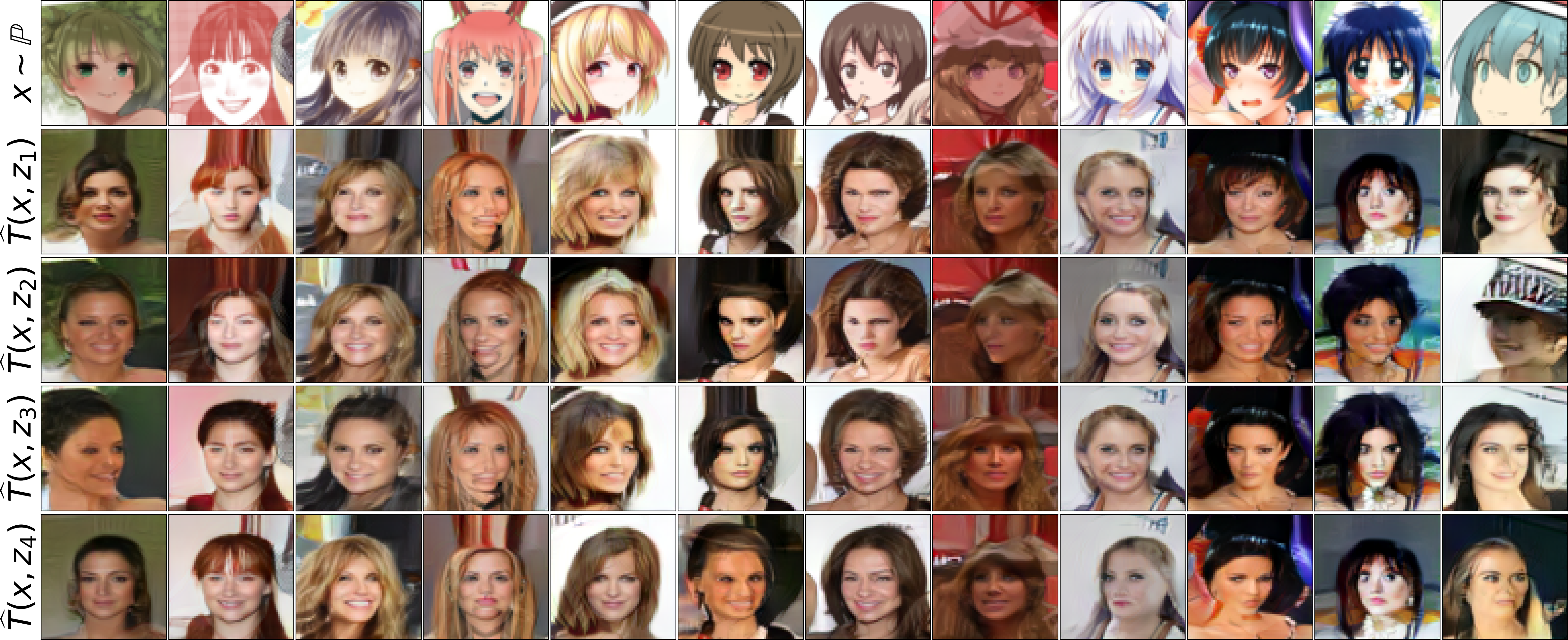
(a) Input images $x$ and random translated examples $T(x,z)$.

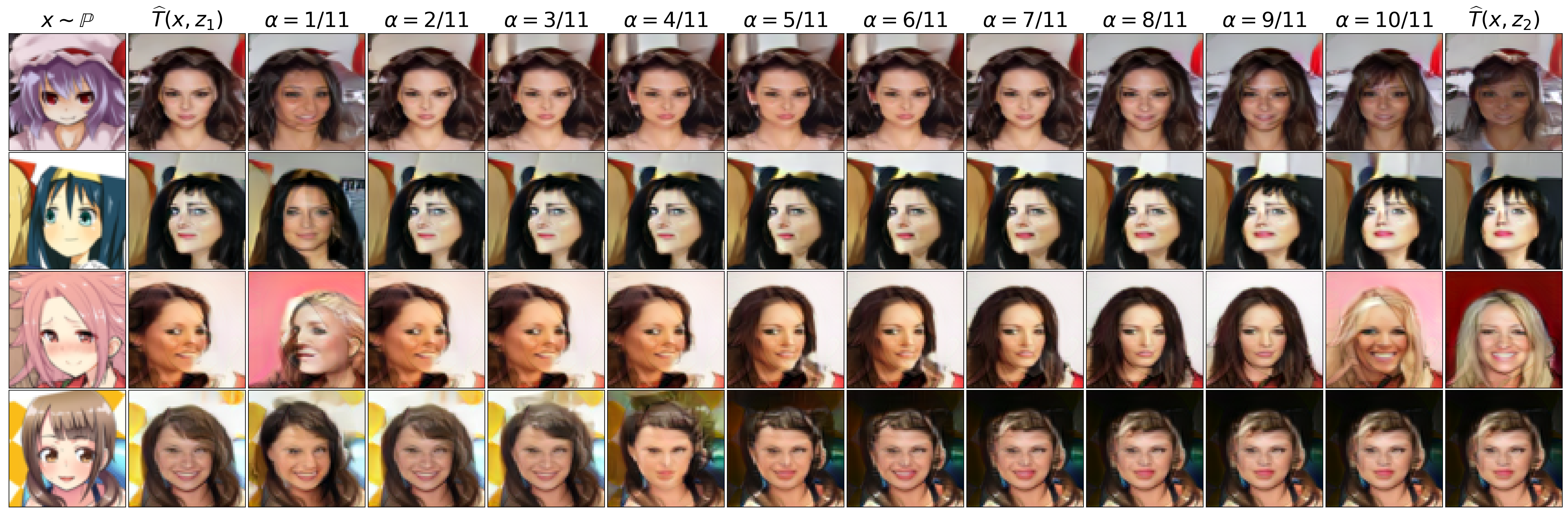
(b) Interpolation in the conditional latent space, $z=(1-\alpha)z_{1}+\alpha z_{2}$.

Figure 20: Anime $\rightarrow$ celeba (female) translation, $64\times 64$, stochastic. Additional examples.

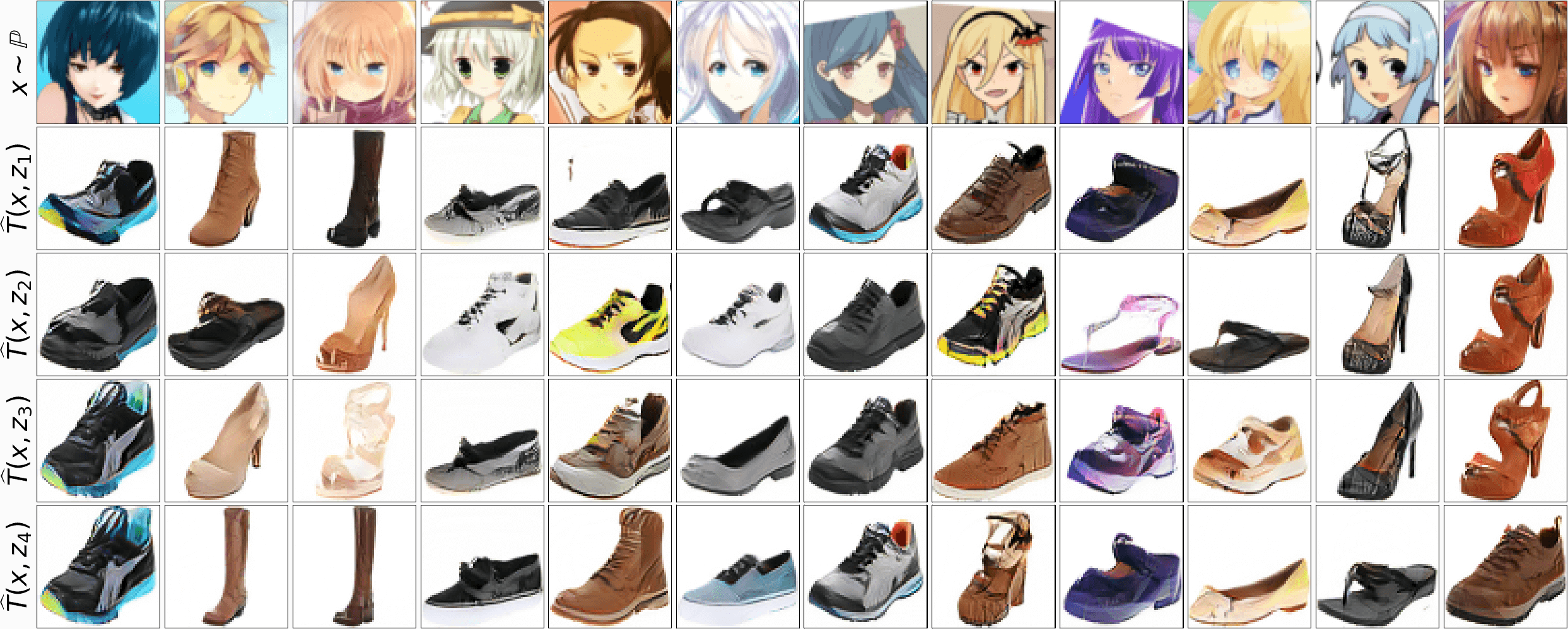
(a) Input images $x$ and random translated examples $T(x,z)$.

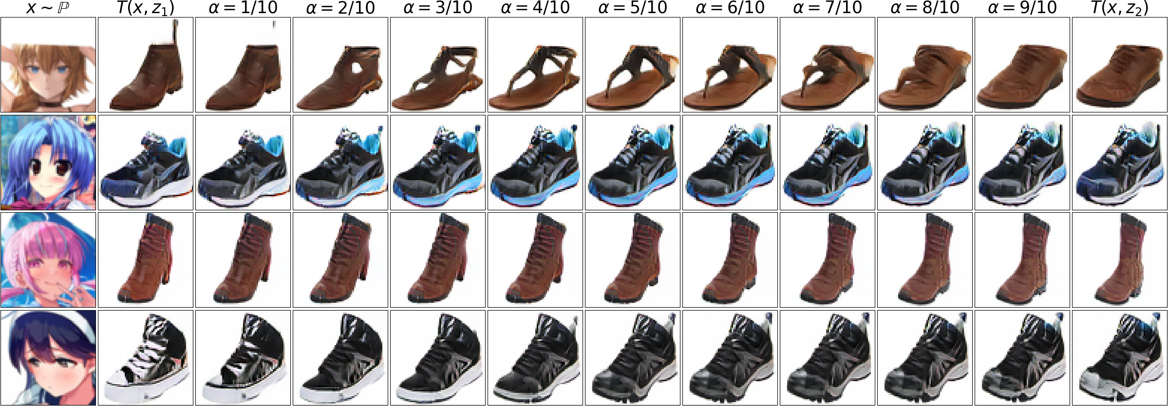
(b) Interpolation in the conditional latent space, $z=(1-\alpha)z_{1}+\alpha z_{2}$.

Figure 21: Anime $\rightarrow$ shoes translation, $64\times 64$, stochastic. Additional examples.

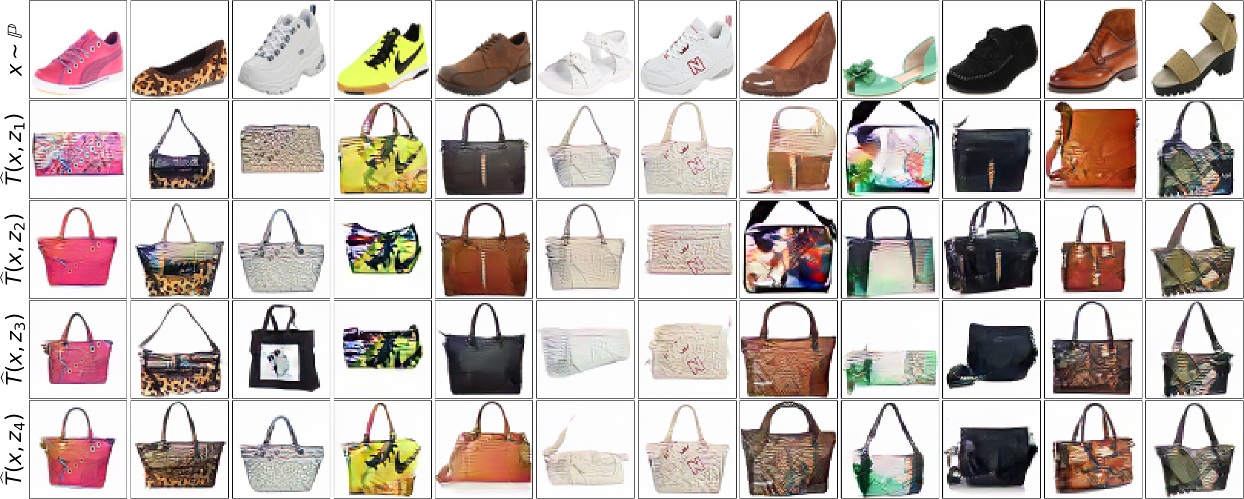
(a) Input images $x$ and random translated examples $T(x,z)$.

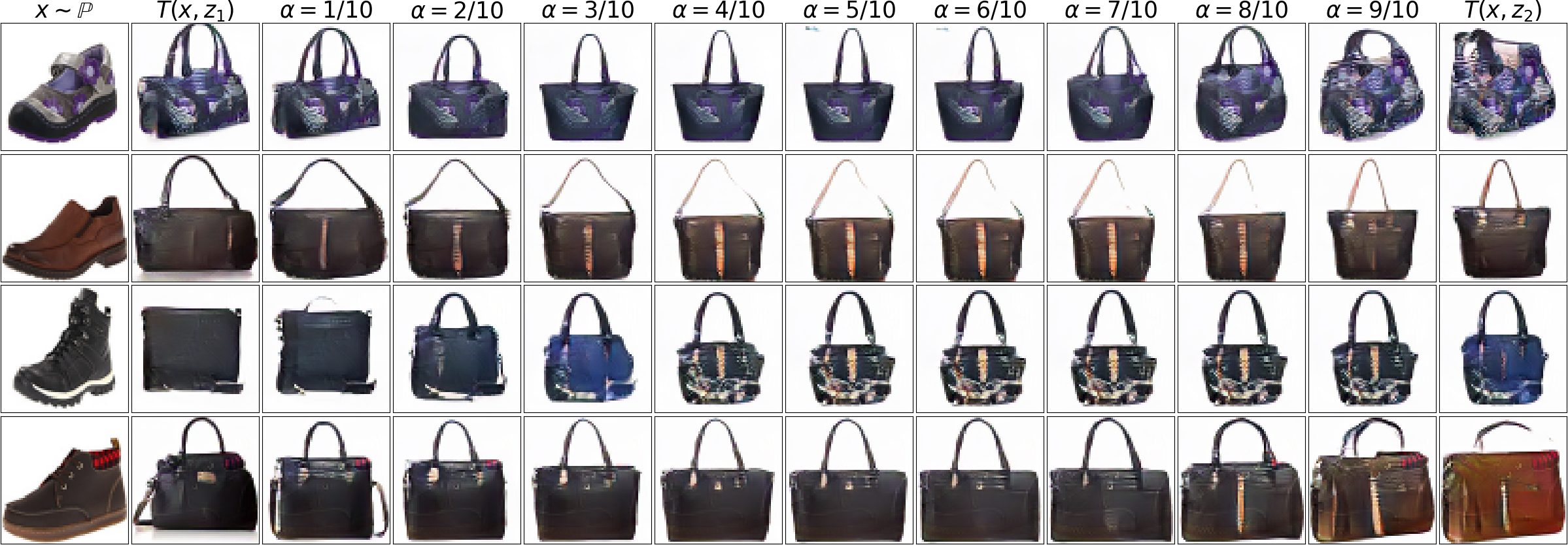
(b) Interpolation in the conditional latent space, $z=(1-\alpha)z_{1}+\alpha z_{2}$.

Figure 22: Shoes $\rightarrow$ handbags, $64\times 64$, stochastic. Additional examples.

Appendix I Examples with the Synchronized Noise

In this section, for handbags$\rightarrow$shoes (64$\times$64) and outdoor$\rightarrow$church (128$\times$128) datasets, we pick a batch of input data $x_{1},\dots,x_{N}\sim\mathbb{P}$ and noise $z_{1},\dots,z_{K}\sim\mathbb{S}$ to plot the $N\times K$ matrix of generated images $T_{\theta}(x_{n},z_{k})$. Our goal is to assess whether using the same $z_{k}$ for different $x_{n}$ leads to some shared effects such as the same form a generated shoe or church.

The images results are given in Figures 23 and 24. Qualitatively, we do not find any close relation between images produced with the same noise vectors for different input images $x_{n}$.

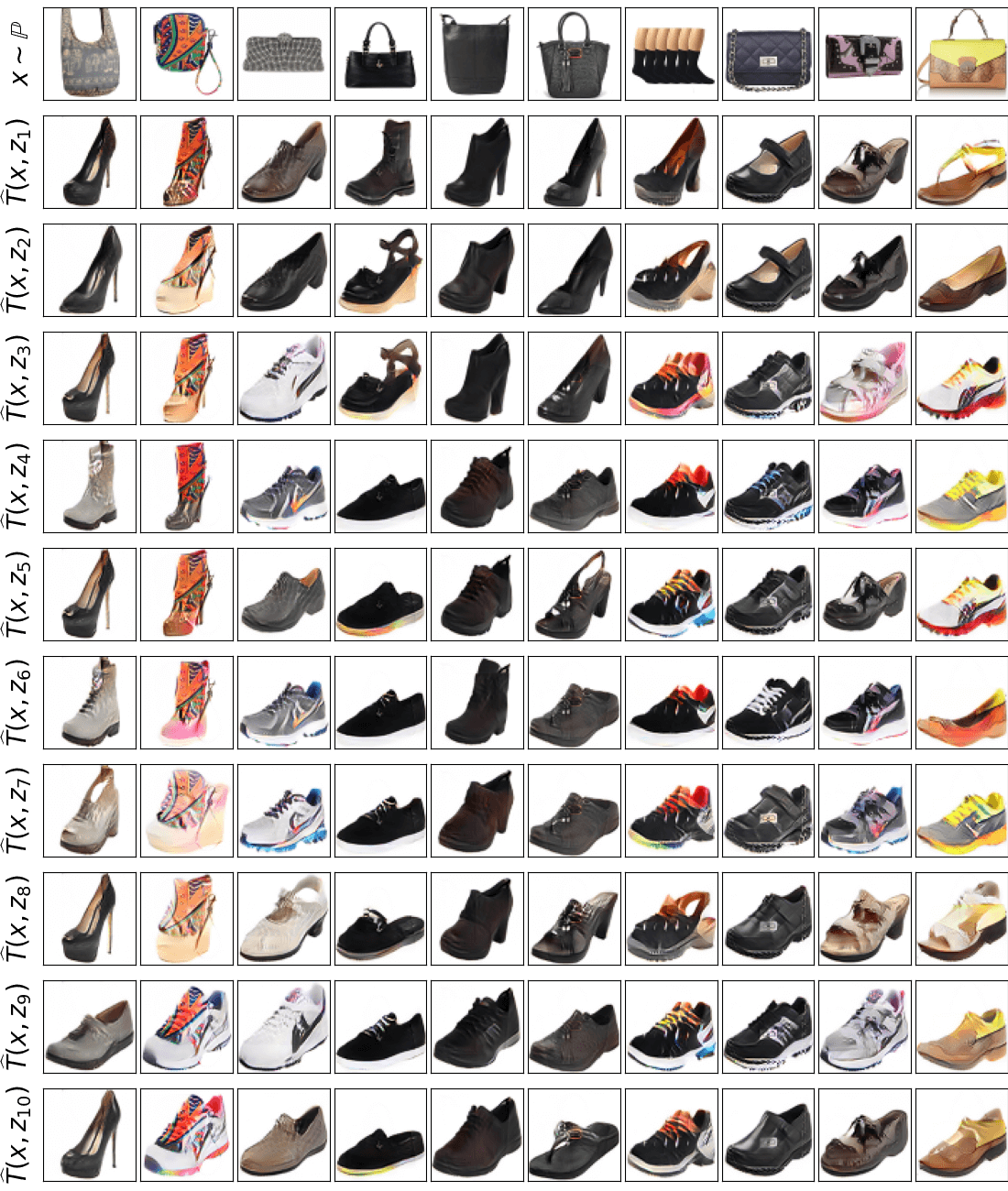
Figure 23: Input images $x$ and random translated examples $T(x,z)$.In this example, noise inputs $z$ are synchronized between different input images $x$.

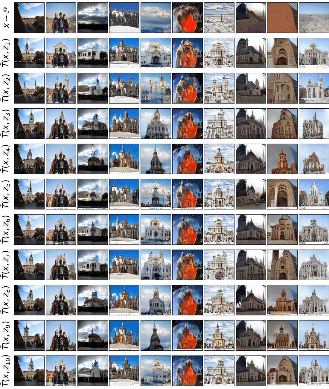
Figure 24: Input images $x$ and random translated examples $T(x,z)$.In this example, noise inputs $z$ are synchronized between different input images $x$.

References

- Alibert et al. (2019) J-J Alibert, Guy Bouchitté, and Thierry Champion. A new class of costs for optimal transport planning. European Journal of Applied Mathematics, 30(6):1229–1263, 2019.
- Almahairi et al. (2018) Amjad Almahairi, Sai Rajeshwar, Alessandro Sordoni, Philip Bachman, and Aaron Courville. Augmented cyclegan: Learning many-to-many mappings from unpaired data. In International Conference on Machine Learning, pp. 195–204. PMLR, 2018.
- Amos et al. (2017) Brandon Amos, Lei Xu, and J Zico Kolter. Input convex neural networks. In Proceedings of the 34th International Conference on Machine Learning-Volume 70, pp. 146–155. JMLR. org, 2017.
- Arjovsky et al. (2017) Martin Arjovsky, Soumith Chintala, and Léon Bottou. Wasserstein generative adversarial networks. In International conference on machine learning, pp. 214–223. PMLR, 2017.
- Backhoff-Veraguas et al. (2019) Julio Backhoff-Veraguas, Mathias Beiglböck, and Gudmun Pammer. Existence, duality, and cyclical monotonicity for weak transport costs. Calculus of Variations and Partial Differential Equations, 58(6):1–28, 2019.
- Benaim & Wolf (2017) Sagie Benaim and Lior Wolf. One-sided unsupervised domain mapping. Advances in Neural Information Processing Systems, 30, 2017.
- Cherian & Sullivan (2019) Anoop Cherian and Alan Sullivan. Sem-gan: semantically-consistent image-to-image translation. In 2019 ieee winter conference on applications of computer vision (wacv), pp. 1797–1806. IEEE, 2019.
- Chizat (2017) Lenaic Chizat. Unbalanced optimal transport: Models, numerical methods, applications. PhD thesis, Université Paris sciences et lettres, 2017.
- Choi et al. (2020) Yunjey Choi, Youngjung Uh, Jaejun Yoo, and Jung-Woo Ha. Stargan v2: Diverse image synthesis for multiple domains. In Proceedings of the IEEE/CVF conference on computer vision and pattern recognition, pp. 8188–8197, 2020.
- Daniels et al. (2021) Grady Daniels, Tyler Maunu, and Paul Hand. Score-based generative neural networks for large-scale optimal transport. Advances in Neural Information Processing Systems, 34, 2021.
- Fan et al. (2022) Jiaojiao Fan, Shu Liu, Shaojun Ma, Yongxin Chen, and Hao-Min Zhou. Scalable computation of monge maps with general costs. In ICLR Workshop on Deep Generative Models for Highly Structured Data, 2022. URL https://openreview.net/forum?id=rEnGR3VdDW5.
- Folland (1999) Gerald B Folland. Real analysis: modern techniques and their applications, volume 40. John Wiley & Sons, 1999.
- Genevay et al. (2016) Aude Genevay, Marco Cuturi, Gabriel Peyré, and Francis Bach. Stochastic optimization for large-scale optimal transport. In Advances in neural information processing systems, pp. 3440–3448, 2016.
- Goodfellow et al. (2014) Ian Goodfellow, Jean Pouget-Abadie, Mehdi Mirza, Bing Xu, David Warde-Farley, Sherjil Ozair, Aaron Courville, and Yoshua Bengio. Generative adversarial nets. In Advances in neural information processing systems, pp. 2672–2680, 2014.
- Gozlan & Juillet (2020) Nathael Gozlan and Nicolas Juillet. On a mixture of brenier and strassen theorems. Proceedings of the London Mathematical Society, 120(3):434–463, 2020.
- Gozlan et al. (2017) Nathael Gozlan, Cyril Roberto, Paul-Marie Samson, and Prasad Tetali. Kantorovich duality for general transport costs and applications. Journal of Functional Analysis, 273(11):3327–3405, 2017.
- Gulrajani et al. (2017) Ishaan Gulrajani, Faruk Ahmed, Martin Arjovsky, Vincent Dumoulin, and Aaron C Courville. Improved training of Wasserstein GANs. In Advances in Neural Information Processing Systems, pp. 5767–5777, 2017.
- Heusel et al. (2017) Martin Heusel, Hubert Ramsauer, Thomas Unterthiner, Bernhard Nessler, and Sepp Hochreiter. GANs trained by a two time-scale update rule converge to a local nash equilibrium. In Advances in neural information processing systems, pp. 6626–6637, 2017.
- Ho et al. (2020) Jonathan Ho, Ajay Jain, and Pieter Abbeel. Denoising diffusion probabilistic models. Advances in Neural Information Processing Systems, 33:6840–6851, 2020.
- Huang et al. (2018) Xun Huang, Ming-Yu Liu, Serge Belongie, and Jan Kautz. Multimodal unsupervised image-to-image translation. In Proceedings of the European conference on computer vision (ECCV), pp. 172–189, 2018.
- Johnson et al. (2016) Justin Johnson, Alexandre Alahi, and Li Fei-Fei. Perceptual losses for real-time style transfer and super-resolution. In European conference on computer vision, pp. 694–711. Springer, 2016.
- Kallenberg (1997) Olav Kallenberg. Foundations of modern probability, volume 2. Springer, 1997.
- Kantorovitch (1958) Leonid Kantorovitch. On the translocation of masses. Management Science, 5(1):1–4, 1958.
- Kidger & Lyons (2020) Patrick Kidger and Terry Lyons. Universal approximation with deep narrow networks. In Conference on learning theory, pp. 2306–2327. PMLR, 2020.
- Kim et al. (2017) Taeksoo Kim, Moonsu Cha, Hyunsoo Kim, Jung Kwon Lee, and Jiwon Kim. Learning to discover cross-domain relations with generative adversarial networks. In International Conference on Machine Learning, pp. 1857–1865. PMLR, 2017.
- Kingma & Ba (2014) Diederik P Kingma and Jimmy Ba. Adam: A method for stochastic optimization. arXiv preprint arXiv:1412.6980, 2014.
- Korotin et al. (2021a) Alexander Korotin, Vage Egiazarian, Arip Asadulaev, Alexander Safin, and Evgeny Burnaev. Wasserstein-2 generative networks. In International Conference on Learning Representations, 2021a. URL https://openreview.net/forum?id=bEoxzW_EXsa.
- Korotin et al. (2021b) Alexander Korotin, Lingxiao Li, Aude Genevay, Justin M Solomon, Alexander Filippov, and Evgeny Burnaev. Do neural optimal transport solvers work? a continuous wasserstein-2 benchmark. Advances in Neural Information Processing Systems, 34, 2021b.
- Korotin et al. (2021c) Alexander Korotin, Lingxiao Li, Justin Solomon, and Evgeny Burnaev. Continuous wasserstein-2 barycenter estimation without minimax optimization. In International Conference on Learning Representations, 2021c. URL https://openreview.net/forum?id=3tFAs5E-Pe.
- Korotin et al. (2022a) Alexander Korotin, Vage Egiazarian, Lingxiao Li, and Evgeny Burnaev. Wasserstein iterative networks for barycenter estimation. In Alice H. Oh, Alekh Agarwal, Danielle Belgrave, and Kyunghyun Cho (eds.), Advances in Neural Information Processing Systems, 2022a. URL https://openreview.net/forum?id=GiEnzxTnaMN.
- Korotin et al. (2022b) Alexander Korotin, Alexander Kolesov, and Evgeny Burnaev. Kantorovich strikes back! wasserstein GANs are not optimal transport? In Thirty-sixth Conference on Neural Information Processing Systems Datasets and Benchmarks Track, 2022b. URL https://openreview.net/forum?id=VtEEpi-dGlt.
- Léonard (2014) Christian Léonard. A survey of the schrödinger problem and some of its connections with optimal transport. Discrete & Continuous Dynamical Systems, 34(4):1533, 2014.
- Liu et al. (2019) Huidong Liu, Xianfeng Gu, and Dimitris Samaras. Wasserstein GAN with quadratic transport cost. In Proceedings of the IEEE International Conference on Computer Vision, pp. 4832–4841, 2019.
- Liu et al. (2017) Ming-Yu Liu, Thomas Breuel, and Jan Kautz. Unsupervised image-to-image translation networks. In Advances in neural information processing systems, pp. 700–708, 2017.
- Liu et al. (2020) Yahui Liu, Marco De Nadai, Jian Yao, Nicu Sebe, Bruno Lepri, and Xavier Alameda-Pineda. Gmm-unit: Unsupervised multi-domain and multi-modal image-to-image translation via attribute gaussian mixture modeling. arXiv preprint arXiv:2003.06788, 2020.
- Liu et al. (2015) Ziwei Liu, Ping Luo, Xiaogang Wang, and Xiaoou Tang. Deep learning face attributes in the wild. In Proceedings of International Conference on Computer Vision (ICCV), December 2015.
- Lu et al. (2019) Guansong Lu, Zhiming Zhou, Yuxuan Song, Kan Ren, and Yong Yu. Guiding the one-to-one mapping in cyclegan via optimal transport. In Proceedings of the AAAI Conference on Artificial Intelligence, volume 33, pp. 4432–4439, 2019.
- Lu et al. (2020) Guansong Lu, Zhiming Zhou, Jian Shen, Cheng Chen, Weinan Zhang, and Yong Yu. Large-scale optimal transport via adversarial training with cycle-consistency. arXiv preprint arXiv:2003.06635, 2020.
- Makkuva et al. (2020) Ashok Makkuva, Amirhossein Taghvaei, Sewoong Oh, and Jason Lee. Optimal transport mapping via input convex neural networks. In International Conference on Machine Learning, pp. 6672–6681. PMLR, 2020.
- Nowozin et al. (2016) Sebastian Nowozin, Botond Cseke, and Ryota Tomioka. f-GAN: Training generative neural samplers using variational divergence minimization. In Advances in neural information processing systems, pp. 271–279, 2016.
- Petzka et al. (2017) Henning Petzka, Asja Fischer, and Denis Lukovnicov. On the regularization of wasserstein gans. arXiv preprint arXiv:1709.08894, 2017.
- Peyré et al. (2019) Gabriel Peyré, Marco Cuturi, et al. Computational optimal transport. Foundations and Trends® in Machine Learning, 11(5-6):355–607, 2019.
- Rockafellar (1976) R Tyrrell Rockafellar. Integral functionals, normal integrands and measurable selections. In Nonlinear operators and the calculus of variations, pp. 157–207. Springer, 1976.
- Rockafellar (1966) Ralph Rockafellar. Characterization of the subdifferentials of convex functions. Pacific Journal of Mathematics, 17(3):497–510, 1966.
- Ronneberger et al. (2015) Olaf Ronneberger, Philipp Fischer, and Thomas Brox. U-net: Convolutional networks for biomedical image segmentation. In International Conference on Medical image computing and computer-assisted intervention, pp. 234–241. Springer, 2015.
- Rout et al. (2022) Litu Rout, Alexander Korotin, and Evgeny Burnaev. Generative modeling with optimal transport maps. In International Conference on Learning Representations, 2022. URL https://openreview.net/forum?id=5JdLZg346Lw.
- Saito et al. (2020) Kuniaki Saito, Kate Saenko, and Ming-Yu Liu. Coco-funit: Few-shot unsupervised image translation with a content conditioned style encoder. In European Conference on Computer Vision, pp. 382–398. Springer, 2020.
- Sanjabi et al. (2018) Maziar Sanjabi, Jimmy Ba, Meisam Razaviyayn, and Jason D Lee. On the convergence and robustness of training gans with regularized optimal transport. Advances in Neural Information Processing Systems, 31, 2018.
- Santambrogio (2015) Filippo Santambrogio. Optimal transport for applied mathematicians. Birkäuser, NY, 55(58-63):94, 2015.
- Seguy et al. (2017) Vivien Seguy, Bharath Bhushan Damodaran, Remi Flamary, Nicolas Courty, Antoine Rolet, and Mathieu Blondel. Large scale optimal transport and mapping estimation. In International Conference on Learning Representations, 2017.
- Su et al. (2023) Xuan Su, Jiaming Song, Chenlin Meng, and Stefano Ermon. Dual diffusion implicit bridges for image-to-image translation. In International Conference on Learning Representations, 2023. URL https://openreview.net/forum?id=5HLoTvVGDe.
- Taghvaei & Jalali (2019) Amirhossein Taghvaei and Amin Jalali. 2-Wasserstein approximation via restricted convex potentials with application to improved training for GANs. arXiv preprint arXiv:1902.07197, 2019.
- Villani (2008) Cédric Villani. Optimal transport: old and new, volume 338. Springer Science & Business Media, 2008.
- Xie et al. (2019) Yujia Xie, Minshuo Chen, Haoming Jiang, Tuo Zhao, and Hongyuan Zha. On scalable and efficient computation of large scale optimal transport. volume 97 of Proceedings of Machine Learning Research, pp. 6882–6892, Long Beach, California, USA, 09–15 Jun 2019. PMLR. URL http://proceedings.mlr.press/v97/xie19a.html.
- Yang & Uhler (2019) Karren D. Yang and Caroline Uhler. Scalable unbalanced optimal transport using generative adversarial networks. In International Conference on Learning Representations, 2019. URL https://openreview.net/forum?id=HyexAiA5Fm.
- Yu & Grauman (2014) Aron Yu and Kristen Grauman. Fine-grained visual comparisons with local learning. In Proceedings of the IEEE Conference on Computer Vision and Pattern Recognition, pp. 192–199, 2014.
- Yu et al. (2015) Fisher Yu, Ari Seff, Yinda Zhang, Shuran Song, Thomas Funkhouser, and Jianxiong Xiao. Lsun: Construction of a large-scale image dataset using deep learning with humans in the loop. arXiv preprint arXiv:1506.03365, 2015.
- Zhang (2018) Yongqi Zhang. Xogan: One-to-many unsupervised image-to-image translation. arXiv preprint arXiv:1805.07277, 2018.
- Zhou et al. (2014) Bolei Zhou, Agata Lapedriza, Jianxiong Xiao, Antonio Torralba, and Aude Oliva. Learning deep features for scene recognition using places database. 2014.
- Zhu et al. (2017a) Jun-Yan Zhu, Taesung Park, Phillip Isola, and Alexei A Efros. Unpaired image-to-image translation using cycle-consistent adversarial networks. In Proceedings of the IEEE international conference on computer vision, pp. 2223–2232, 2017a.
- Zhu et al. (2017b) Jun-Yan Zhu, Richard Zhang, Deepak Pathak, Trevor Darrell, Alexei A Efros, Oliver Wang, and Eli Shechtman. Toward multimodal image-to-image translation. Advances in neural information processing systems, 30, 2017b.