Spectral study of the diffuse synchrotron source in the galaxy cluster Abell 523

Abstract

The galaxy cluster Abell 523 (A523) hosts an extended diffuse synchrotron source historically classified as a radio halo. Its radio power at 1.4 GHz makes it one of the most significant outliers in the scaling relations between observables derived from multi-wavelength observations of galaxy clusters: it has a morphology that is different and offset from the thermal gas, and it has polarized emission at 1.4 GHz typically difficult to observe for this class of sources. A magnetic field fluctuating on large spatial scales ($\sim$1 Mpc) can explain these peculiarities but the formation mechanism for this source is not yet completely clear. To investigate its formation mechanism, we present new observations obtained with the LOw Frequency ARray at 120-168 MHz and the Jansky Very Large Array at 1-2 GHz, which allow us to study the spectral index distribution of this source. According to our data the source is observed to be more extended at 144 MHz than previously inferred at 1.4 GHz, with a total size of about 1.8 Mpc and a flux density $S_{\rm 144\,MHz}=(1.52\pm 0.31)$ Jy. The spectral index distribution of the source is patchy with an average spectral index $\alpha\sim 1.2$ between 144 MHz and 1.410 GHz, while an integrated spectral index $\alpha\,\sim\,2.1$ has been obtained between 1.410 GHz and 1.782 GHz. A previously unseen patch of steep spectrum emission is clearly detected at 144 MHz in the south of the cluster. Overall, our findings suggest that we are observing an overlapping of different structures, powered by the turbulence associated with the primary and a possible secondary merger.

1 Introduction

Diffuse synchrotron sources observed in merging galaxy clusters indicate the presence of ultra-relativistic electrons ($\gamma>>1000$) spiralling along the flux lines of weak magnetic fields ($\sim\mu$G), and can be classified as (giant) halos and relics (e.g., Feretti et al., 2012; Brunetti & Jones, 2014; Vacca et al., 2018a; van Weeren et al., 2019).

Radio halos have been observed in a fraction of massive and disturbed galaxy clusters where they fill the central volume of the system (Cassano et al., 2010). The prototype and most famous radio halo is Coma C which resides in the Coma cluster and was first observed by Large et al. (1959). Overall, radio halos extend up to spatial scales of $\sim$1-2 Mpc and are characterized by low radio brightness ($\sim$0.1 $\mu$Jy/arcsec² at 1.4 GHz). Out of about 100 radio halos presently confirmed, three show filaments of polarized emission at around 20% at 1.4 GHz (A2255 Govoni et al. 2005, MACS J0717.5+3745 Bonafede et al. 2009, and A523 Girardi et al. 2016). These are likely projected on the cluster center as suggested by recent studies of A2255 and MACS J0717.5+3745 (Pizzo et al., 2011; Botteon et al., 2020; Rajpurohit et al., 2020). Moreover, a 5$\sigma$ upper limit of 13% on the fractional polarization has been derived for the radio halo in 1E 0657-55.8 by Shimwell et al. (2014). Three-dimensional numerical simulations suggest that radio halos are intrinsically polarized at 1.4 GHz, with filaments of polarized emission expected to be observed at distances greater than 1.5 Mpc from the cluster center, reflecting the intracluster magnetic field structure (Loi et al., 2019). However, the resolution and sensitivity of present instruments hinder the detection of this polarized emission in most radio halos (Govoni et al., 2013).

Typically, most powerful and extended radio halos are hosted in massive and bright X-ray clusters and show strong correlation between the integrated radio halo emission at 1.4 GHz and the X-ray luminosity of the intracluster medium (ICM) and galaxy cluster mass (e.g., Liang et al., 2000; Cassano et al., 2013; Yuan et al., 2015; Cuciti et al., 2021). Exceptions have been observed of radio halos that show a radio power at 1.4 GHz larger than expected from the radio power ($P_{\rm 1.4\,GHz}$) - X-ray luminosity ($L_{\rm X,0.1-2.4\,keV}$) correlation holding for the most of radio halos, one of the most significant being the source in A523 (Giovannini et al., 2011).  Detailed studies indicate, in some cases, a point-to-point correlation between the X-ray and radio brightness at 1.4 GHz as, e.g., for the radio halos in the Coma cluster and 1RXS  J0603.3+4214 (Govoni et al., 2001a; Brown & Rudnick, 2011; Rajpurohit et al., 2018), while a minor (e.g., A520 Govoni et al. 2001b; Hoang et al. 2019) or absent (e.g., 1E 0657-55.8 Shimwell et al. 2014) correlation has been found in other clusters.

Radio relics are elongated diffuse synchrotron sources with filamentary morphology that are observed in the periphery of a number of merging galaxy clusters. Sometimes they come in pairs along the merger axis but on opposite sides (e.g., Rottgering et al., 1997; Bagchi et al., 2006; van Weeren et al., 2011) and/or coexist with cluster radio halos (e.g., Brown et al., 2011; Lindner et al., 2014; Parekh et al., 2017). They are extended on spatial scales of $\sim$0.5-2 Mpc, are characterized by low radio surface brightness ($\sim$0.1 $\mu$Jy/arcsec² at 1.4 GHz), and are highly polarized at GHz frequencies with fractional polarization larger than 20% at 1.4 GHz.

In our present understanding, a key role in the origin of radio halos and relics is likely played by cluster merger phenomena in the form of turbulence and shocks. Merger-induced turbulence is thought to accelerate a pre-existing electron population (seed population) through the Fermi-II mechanism, giving rise to diffuse synchrotron sources filling the central volume, i.e. radio halos, of a fraction of massive galaxy clusters. According to this scenario, a variety of spectra and spectral trends are expected (see, e.g. Brunetti & Jones, 2014). Compelling evidence is now available that directly links radio relics with cluster shocks observed at X-rays and mm/sub-mm wavelengths (e.g., Akamatsu et al., 2013; Planck Collaboration et al., 2013; Erler et al., 2015; Eckert et al., 2016; Urdampilleta et al., 2018). According to these findings, the emission observed in radio seems to be explained if cosmic-ray electrons are accelerated up to $\sim$GeV energies through diffusive shock acceleration (DSA Drury, 1983; Blandford & Ostriker, 1978) either from the thermal pool, as proposed first by Ensslin et al. (1998), or from supra-thermal/relativistic plasma (e.g., Markevitch et al. 2005 and Kang et al. 2012).

Precious insights on the origin of these sources come from the spectral analysis of their properties over a wide frequency range and from the comparison of observations with theoretical expectations and simulations. Radio halos are characterized by steep-spectra ($S_{\nu}\propto\nu^{-\alpha}$, with $\alpha\simeq$1-1.4, where $S_{\nu}$ is the flux density at the observing frequency $\nu$ and $\alpha$ is the spectral index). Detailed spatially-resolved spectral index images have been produced for a number of radio halos, revealing different behaviours. Indications of radial steepening have been found in a few clusters (e.g., Giovannini et al., 1993; Feretti et al., 2004; Pearce et al., 2017), while other radio halos show no clear trend with either uniform (e.g., Vacca et al., 2014; Rajpurohit et al., 2018; Hoang et al., 2019) or complex (e.g., Giacintucci et al., 2005; Orrú et al., 2007; Kale & Dwarakanath, 2010; Shimwell et al., 2014; Rajpurohit et al., 2020; Botteon et al., 2020) distributions. Radio relics are also characterized by steep-spectra ($\alpha\simeq$1-1.5), and detailed spectral index images show a steepening transversely to their elongation towards the cluster center (e.g., Clarke & Ensslin, 2006; de Gasperin et al., 2015; Di Gennaro et al., 2018). The steepening is interpreted as synchrotron and inverse Compton losses in the shock downstream region.

In this paper we present new 144 MHz LOw Frequency ARray (LOFAR) observations and new 1-2 GHz Jansky Very Large Array (VLA) observations of the galaxy cluster A523 which hosts a powerful diffuse source associated with the ICM, historically classified as a radio halo. Its radio power at 1.4 GHz makes it one of the most significant outliers in the scaling relations between observables derived from multi-wavelength observations of galaxy clusters: it has a morphology that is different and offset from the thermal gas, and it has polarized emission at 1.4 GHz typically difficult to observe for this class of sources. We study the spectral behaviour of the emission between 144 MHz and 2 GHz to better understand the formation mechanism of this source and compare the radio emission with observations at X-ray wavelengths. In §2 we summarize the present knowledge on this cluster, in §3 we describe the data used for the analysis. In §4 we present the new images of the cluster, in §5 the spectral behaviour and in §6 a comparison between the radio and X-ray derived cluster properties. Finally, in §7 and in §8 we discuss the nature of the system and draw our conclusions. Throughout, we use a $\Lambda$CDM cosmology with $H_{0}=67.4$ km/s/Mpc, $\Omega_{0}=0.315$ and $\Omega_{\Lambda}=0.685$ (Planck Collaboration et al., 2020). With this cosmology, at the distance of A523 ($z=0.104$, luminosity distance 499 Mpc), $1^{\prime\prime}$ corresponds to 1.98 kpc.

Table 1: Radio observations used in this work.

RA	Dec	Instrument	$\nu$	Bandwidth	Config.	Date	Duration	Project
h:m:s	∘:′:′′		(MHz)	(MHz)			(h)
(J2000)	(J2000)
04:57:06.3	+08:56:53.7	LOFAR	144	48	HBA DUAL	31-10-2018	4	LC10$\_$024
04:57:06.3	+08:56:53.7	LOFAR	144	48	HBA DUAL	11-10-2018	4	LC10$\_$024
04:59:10.0	+08:49:00.0	VLA	1.5	1000	C	06-07-2013	1.1	13A-168
04:59:10.0	+08:49:00.0	VLA	1.5	1000	D	29-01-2013	1.1	13A-168

2 The galaxy cluster A523

A523 is a nearby cluster ($z=0.1040\pm 0.0004$, Girardi et al. 2016) with an estimated $M_{\rm X,500}\approx 2.2-3.6\times 10^{14}M_{\odot}$ Cova et al. 2019, where $M_{\rm X,500}$ is the mass derived from X-observables within $R_{\rm 500}$. A523 is a disturbed system with an ongoing merger along the SSW-NNE direction between two subclusters (Girardi et al., 2016; Golovich et al., 2019). A secondary merger is likely present along the ESE-WNW direction (Cova et al., 2019). The cluster is known to host a powerful extended synchrotron source, classified as a radio halo because it permeates both the merging clumps and does not show transverse flux asymmetry typical of radio relics (Giovannini et al., 2011). Girardi et al. (2016) derived a flux density of the source at 1.4 GHz of $72\pm 3$ mJy. According to Einasto et al. (2001), A523 belongs to the supercluster SCL 62 that includes the clusters A525, A515, A529, A532, all of which lie at a similar redshift. In this context, the supercluster has been recently targeted to search for diffuse emission in and beyond galaxy clusters with the Sardinia Radio Telescope (SRT) by Vacca et al. (2018b) who found patches of diffuse emission of unknown origin. A fraction of these turned out to be Galactic H-$\alpha$ regions and blending of discrete sources (Hodgson et al., 2020). Follow up studies are still in progress for the remaining regions.

A detailed multi-wavelength study including optical, X-ray, and radio data at 1.4 GHz has enabled an accurate characterization of the cluster dynamical and non-thermal properties, revealing that the radio halo emission is mainly elongated perpendicular to the merging axis defined by the optical and X-ray observations, with a clear offset between the peaks of the radio and the X-ray brightness distribution of about 310 kpc (Girardi et al., 2016). Unlike other radio halos, the source in A523 does not show a strong point-to-point correlation between the 1.4 GHz radio and X-ray brightness distribution but it is rather characterized by a broad intrinsic scatter between these two quantities (Cova et al., 2019). Overall, its radio power at 1.4 GHz is $P_{\rm 1.4\,GHz}=2.2\times 10^{24}$ W/Hz, while the X-ray luminosity is $L_{\rm X,500[0.1-2.4]}=1.5\times 10^{44}$ erg/s (Girardi et al., 2016; Cova et al., 2019). The 1.4 GHz radio emission appears to be higher by a factor $\sim 6-18$ than expected from the X-ray luminosity of the system according to the best-fit scaling relations presented in Yuan et al. (2015). We use for the redshift of this cluster $z=0.1040\pm 0.0004$ (Girardi et al., 2016), derived through a detailed optical study based on 132 spectroscopic redshifts of which 80 related to cluster members and later confirmed by Golovich et al. (2019). This makes it very unlikely that an incorrect estimate of the redshift could be the reason of the higher radio power.

It might be that the cluster emission is overly bright in the radio because of a third subcluster merging in the direction perpendicular to the main merger and causing additional turbulence, as proposed by Cova et al. (2019) on the basis of new XMM-Newton and Nustar observations. Other clusters undergoing multiple mergers have been found to host radio halos, but these radio halos are not over-luminous in radio with respect to X-rays (e.g., Bonafede et al., 2009). The peculiarity of A523 is apparent also in its location on the $P_{\rm 1.4\,GHz}$ - $M_{\rm X,500}$ correlation. By considering the $P_{\rm 1.4\,GHz}$-$M_{\rm X,500}$ correlation for radio halos found by Yuan et al. (2015), we derive a mass $M_{\rm X,500}\,\approx\,6-10\,\times\,10^{14}\,M_{\odot}$, larger than the estimated mass by Cova et al. (2019) even when the uncertainties in the radio power and in the correlation have been taken into account.

A strongly polarized signal ($\sim 15-20\%$), associated with the radio halo, has been detected by Girardi et al. (2016) across most of the radio halo extension. Numerical three-dimensional simulations demonstrate that an intracluster magnetic field with a strength $\langle B_{0}\rangle\simeq 0.5\,\mu$G at the center of the cluster and fluctuating over a range of scales between a few kpc up to 1 Mpc is consistent with both the total intensity and polarized emission of the radio halo (Girardi et al., 2016). The magnetic field has been constrained by the fractional polarization of the diffuse emission, and is therefore relatively independent of the relativistic electron population. Such a magnetic field auto-correlation scale is much larger than the resolution of radio observations ($\sim$130 kpc), preventing the beam depolarization of the radio signal that usually hinders the detection of radio halo polarized emission (Govoni et al., 2013). The value of the magnetic field strength derived by Girardi et al. (2016) is consistent with the results from upper limits on inverse Compton emission of the cluster by Cova et al. (2019), who derive a magnetic field larger than 0.2 $\mu$G over the whole radio halo region and larger than 0.8 $\mu$G when only the brightest region is considered.

3 Radio observations and data reduction

For our analysis, we use new LOFAR data at 120-168 MHz and new VLA observations in the frequency range 1-2 GHz, as described in the following subsections.

3.1 LOFAR observations

We present LOFAR data (SAS ID 682162,672474) obtained through the observing program LC10_024 (PI V. Vacca). A summary of the observations is reported in Table 1. The observations have been carried out with the instrument in interferometer mode in the HBA Dual Inner configuration, with the full (core, remote and international stations) LOFAR array. The study presented in this paper is based on the data from the core and remote stations only. We used a 48 MHz (120-168 MHz) bandwidth with a total of 231 sub-bands per beam. The observations exploit the multi-beam capability of the HBA and were conducted together with the LoTSS observations through the co-observing program offered by the observatory. The observations presented here correspond to the LoTSS pointing P074+09. Due to the low declination of the source ($\sim 8.8^{\circ}$), the observation has been split in two 4 h-blocks to ensure the elevation of the target is higher than 30^∘ throughout the observation.

Table 2: Details of the radio brightness images presented in this work. Col. 1, 2: central frequency and bandwidth; Col. 3: uv-range; Col. 4: resolution; Col. 5: maximum angular scale accessible with the observations; Col. 6: sensitivity; Col. 7: robust; Col. 8: figure/table where the image has been used.

Frequency	Bandwidth	uv-range	Beam	Max scale	$\sigma$	Robust	Figure/Table
MHz	MHz	$\lambda$	${\prime\prime}\times{\prime\prime}$	${\circ}$	mJy/beam
144	48	all	9$\times$9	1.2	0.35	-0.5	Fig. 1
144	48	980- 16980	13.5$\times$13.5	0.06	0.5	-1	Table 3
144	48	all	20$\times$20	1.2	0.4	-0.5	Fig. 2
144	48	158-16980	20$\times$20	0.36	0.45	-0.5	Fig. 5
144	48	all	65$\times$65	1.2	1.3	-0.5	Fig. 3
144	48	158-4835	65$\times$65	0.36	0.9	-0.5	Fig. 5
144	48	196-4835	65$\times$65	0.29	0.9	-0.5	Fig. 4
1410	192	980- 16980	13.5$\times$13.5	0.06	0.09	-1	Table 3
1410	192	158-16980	20$\times$20	0.36	0.075	-0.5	Fig. 5
1410	192	all	65$\times$65	0.36	0.14	0.5	Fig. 3
1410	192	158-4835	65$\times$65	0.36	0.13	-0.5	Fig. 5
1410	192	196-4835	65$\times$65	0.29	0.12	-0.5	Fig. 4
1782	320	980- 16980	13.5$\times$13.5	0.06	0.08	-1	Table 3
1782	320	all	65$\times$65	0.29	0.11	0.5	Fig. 3
1782	320	196-4835	65$\times$65	0.29	0.11	-0.5	Fig. 4

To solve for the complex gains, and to calibrate the bandpass and amplitude, a direction-independent calibration step has been done. The non-directional calibration includes radio frequency interference (RFI) and bright off-axis source removal, as well as clock-total electron content separation based on the calibrator data (see e.g., van Weeren et al., 2016a). During this step the calibrators J0813+4813 (3C196) and J0542+4951 (3C147) have been used as reference respectively for each of the two observing blocks. Direction-independent calibration of the data has been done with pre-factor that takes 1 s and 16 ch/sb and averages down to 8 s and 2 ch/sb (van Weeren et al., 2016a; de Gasperin et al., 2019). These direction-independent calibrated datasets have then been processed with the direction-dependent ddf-pipeline used by the LOFAR Surveys Key Science Project (KSP) for reduction of the LoTSS survey (Tasse et al., 2021). The ddf-pipeline is based on DDFacet (Tasse et al., 2018) and KillMS (Tasse, 2014a, b; Smirnov & Tasse, 2015) and repeats several iterations of direction-dependent self-calibration towards 45 directions of the sky (i.e. facets), with an inner cut on the recorded visibilities of 0.1 km, corresponding to $\sim$48 $\lambda$ at the central frequency of the observations. Shorter baselines have been excluded because of RFI. We performed a further refining of the data in the region where the cluster is located through amplitude and phase self-calibration. Flux contributions from sources outside a square box with sides of length 0.4^∘ centered at approximately the location of the X-ray peak of the cluster (RA 04h:59m:07s and Dec 08^∘:45^′:00^′′) have been subtracted in the uv plane using the direction-dependent calibrations and final ddf-pipeline model, a phase-shift has been applied to locate the target in the phase center, and finally a correction for the LOFAR station beam towards this direction has been applied (this procedure is detailed in van Weeren et al. 2021). We reimage the data that are calibrated in the direction of our target using wsclean-2.10 (Offringa et al., 2014). A post-processing step, summarised in Hardcastle et al. (2021) and which will be described in more detail in Shimwell et al. in prep., was used to scale the wide-field image of our pointing to align the fluxes with the same technique used for LoTSS-DR2 which is itself aligned with the 6C survey (Hales et al., 1988; Hales et al., 1990) through a comparison with the NRAO VLA Sky Survey (NVSS, Condon et al., 1998). The flux scale of the extracted data which, as described above, underwent further processing, was then aligned with the wide field by applying an overall multiplicative factor of 1.720 to the final images made from the extracted data to ensure alignment consistent with the flux scaling strategy used for the LoTSS Data Release 2.

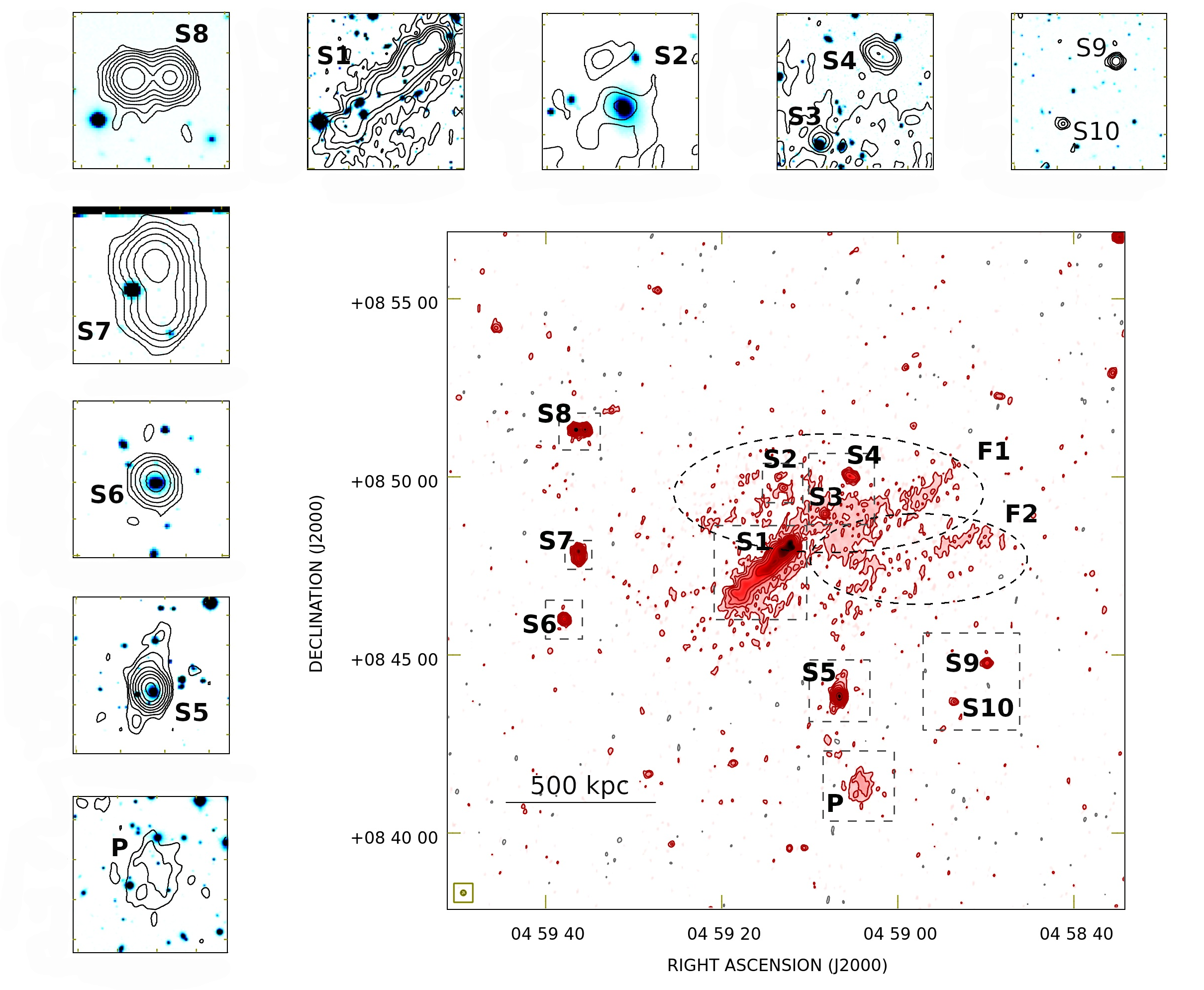
Figure 1: Main panel: LOFAR high-resolution image ($9^{\prime\prime}\times 9^{\prime\prime}$) of the central region of the galaxy cluster A523 in contours and colors. Red contours start at 3$\sigma$ ($\sigma$ = 0.35 mJy/beam) and scale by a factor 2, gray contours are drawn at -3$\sigma$. The horizontal black bar corresponds to 500 kpc at the chosen cosmology and the synthesised beam is shown in the bottom left. The dashed ellipses identify the position of the two filaments F1 and F2. Left and top panels: Zoom on the discrete sources in the field where the radio contours at 9^′′ are superimposed on the optical image from the INT r-band by Girardi et al. (2016), see the text for more details. Positive radio contours are the same as in the large panel. The position of the small panels is marked in the main panel by dashed gray boxes.

In order to investigate the emission from discrete sources as well as from the radio halo, we produced images at low- and high-spatial resolution. At this declination the beam is not circular and, in order to better compare our results with 1.4 GHz observations we convolved the high resolution image with a circular beam of 9^′′ and 13.5^′′, while circular beams of 20^′′ and 65^′′ have been used to restore the images at lower resolution. We note that these images have been produced including all baselines starting from 48 $\lambda$. Shorter baselines have been excluded because of RFI, as noted above. Details about the images presented in the following are given in Table 2. In the following, we assume an uncertainty on the LOFAR flux density scale of 20%, as done for LoTSS (Shimwell et al., 2019).

3.2 VLA observations

We present new VLA data in the frequency range 1-2 GHz in C and D configuration obtained with a mosaic of six pointings in the context of the observing program 13A-168 (PI M. Murgia). The details of the observations are reported in Table 1. The data were reduced following standard procedures using the NRAO’s Astronomical Image Processing System (AIPS) package. The data were collected in spectral line mode in full Stokes, with a total initial bandwidth of 1 GHz subdivided in 16 spectral windows. Each spectral window is 64 MHz wide with 64 channels, and Hanning smoothing was applied before bandpass calibration. The source J0319+4130 (3C84) was used as a bandpass and polarization leakage calibrator, the source J0137+3309 (3C48) was used as a flux density calibrator, and the nearby source J0459+0229 was observed for complex gain calibration. The flux density scale by Perley & Butler (2017) was adopted. RFI flagging has been applied by excision of data with values clearly exceeding the source flux ($\gtrsim 600$ mJy). Following calibration, the data were spectrally averaged to 16 channels of 4 MHz per 64 MHz wide spectral window. Spectral windows from 0 to 5, 9 and 10 were too severely affected by RFI to provide useful information, so we disregard them in the following.

Surface brightness images were produced using the Common Astronomy Software Applications (CASA) package (task tclean). The final images have been produced using spectral windows from 6 to 8 and from 11 to 15, including the full uv-range available, unless differently stated. Circular restoring beams of 13.5^′′, 20^′′ and 65^′′ were used to restore the images in C, C+D, and in D configurations, respectively. Details about the images presented in the following are given in Table 2. In the following, we assume an uncertainty on the VLA flux density scale of 2.5%, in agreement with Perley & Butler (2013).

Everywhere in the text, unless differently stated, the overall uncertainties on the radio brightness and flux density include both the statistical uncertainty and the appropriate uncertainty in the flux density scale.

4 Continuum images

In Fig. 1 we show the 144 MHz cluster emission with 9^′′ resolution. A number of radio galaxies, labelled S1-S10, are present in the field embedded in the diffuse emission and with peaks in the radio brightness higher than 8 $\sigma$. Zoom in’s on these radio galaxies are shown in the left and top panels, where the radio contours are superimposed on the optical image from the Isaac Newton Telescope (INT) r-band by Girardi et al. (2016). These authors identify the head tail S1 with the member-galaxy ID 68, S3 with a point-like source with unknown redshift, S4 with a likely background galaxy, and S5 with the second BCG of the cluster. Using the optical information from the same authors, S2 appears to be the radio counterpart of the brightest cluster galaxy, previously undetected in radio, and S6 the dominant galaxy in the galaxy population of the ESE region, likely in the background at z$\sim$0.14.

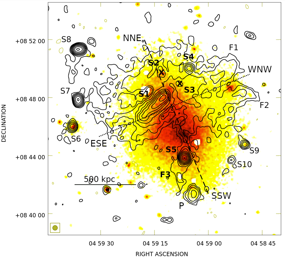
Figure 2: Radio emission from the galaxy cluster A523 at 144 MHz with LOFAR at 20^′′. Black contours start at 3$\sigma$ ($\sigma=$0.4 mJy/beam) and scale by a factor 2, while negative 3$\sigma$ contours are drawn in army green. The beam is shown in the bottom left of the image and the horizontal black bar corresponds to 500 kpc at the chosen cosmology. The radio emission is overlaid on the X-ray image of the cluster from XMM-Newton (Cova et al., 2019), see the text for more details. The dashed and the dotted lines show respectively the axis of the primary and of the secondary merger.

Two filaments of size $\sim$ 6${}^{\prime}\,\times\,1^{\prime}$ (corresponding to about 710 kpc $\times$ 120 kpc) and with higher surface brightness than their surrounding regions of radio emission can be identified and are labelled respectively F1 and F2 (see dashed ellipses in Fig. 1). F1 occupies the region to the north-west of S1, with a few embedded radio sources (S2, S3, S4). F2 is located west of the central AGN S1. No other similar structures are seen elsewhere in the image, suggesting that these filaments are unlikely to be artefacts related to calibration or imaging but rather are real structures. Further south, a new roundish patch of emission, labelled P, is detected at RA 04h59m04s and Dec 08^∘41^′21^′′, with an average brightness that is higher than the brightest regions of the filaments.

Table 3: Spectral index of point sources embedded in the diffuse emission. Col. 1: Source name (see Fig. 1); Col. 2,3: RA and Dec corresponding to the peak of the source at 144 MHz; Col. 4, 5, 6: Flux density at 144 MHz, 1.410 GHz, and 1.782 GHz respectively (this work); Col. 7: Spectral index derived from the flux density values at 144 MHz and 1.410 GHz (this work); Col. 8, 9, 10: Flux density from TGSS (147 MHz) and NVSS (1.4 GHz) and the corresponding spectral index as given by de Gasperin et al. (2018).

Source	RA (J2000)	Dec (J2000)	$S_{\rm 144\,MHz}$	$S_{\rm 1.410\,GHz}$	$S_{\rm 1.782\,GHz}$	$\alpha$	$S_{\rm TGSS}$	$S_{\rm NVSS}$	$\alpha_{\rm dG18}$
	hh:mm:ss	∘:′:′′	mJy	mJy	mJy		mJy	mJy
S1	04:59:12.3	+08:48:04	971.981 $\pm$ 194.43	104.191 $\pm$ 2.68	89.25 $\pm$ 2.30	0.98 $\pm$ 0.09	688.03$\pm$ 13.90	121.71$\pm$1.22	0.77 $\pm$ 0.01
S2	04:59:13.0	+08:49:41	5.81 $\pm$ 1.17	0.54 $\pm$ 0.03	0.23 $\pm$ 0.02	1.04 $\pm$ 0.09	-	-	-
S3	04:59:08.3	+08:48:58	10.88 $\pm$ 2.18	1.04 $\pm$ 0.04	0.93 $\pm$ 0.03	1.03 $\pm$ 0.09	-	-	-
S4	04:59:05.4	+08:50:01	32.48 $\pm$ 6.50	4.44 $\pm$ 0.11	4.55 $\pm$ 0.12	0.87 $\pm$ 0.09	-	-	-
S5	04:59:06.6	+08:43:50	313.68 $\pm$ 62.74	61.74 $\pm$ 1.54	55.84 $\pm$ 1.40	0.71 $\pm$ 0.09	213.91 $\pm$11.10	61.33$\pm$ 1.01	0.55 $\pm$ 0.02
S6	04:59:37.9	+08:46:01	34.65 $\pm$ 6.93	6.91 $\pm$ 0.17	5.78 $\pm$ 0.15	0.71 $\pm$ 0.09	0.0$\pm$ 0.0	6.11$\pm$ 1.02	0.52 $\pm$ 0.00
S7	04:59:36.3	+08:47:54	112.34 $\pm$ 22.47	10.87 $\pm$ 0.27	8.20 $\pm$ 0.21	1.02 $\pm$ 0.09	77.54$\pm$11.05	8.69$\pm$ 1.02	0.97 $\pm$ 0.09
S8	04:59:36.5	+08:51:20	238.71 $\pm$ 47.74	22.14 $\pm$ 0.57	17.35 $\pm$ 0.44	1.04 $\pm$ 0.09	144.93$\pm$ 11.41	19.54$\pm$ 1.00	0.89 $\pm$ 0.04
S9	04:58:49.9	+08:44:46	16.27 $\pm$ 3.26	3.21 $\pm$ 0.09	2.83 $\pm$ 0.07	0.71 $\pm$ 0.09	0.0 $\pm$0.0	5.30$\pm$ 1.00	0.68 $\pm$ 0.00
S10	04:58:53.6	+08:43:41	4.87 $\pm$ 0.98	0.44 $\pm$ 0.02	0.48 $\pm$ 0.02	1.05 $\pm$ 0.09	-	-	-
1 These flux density values include the contribution of the diffuse emission that amounts to about 35 mJy at 144 MHz and to about 2 mJy at 1.4 GHz.

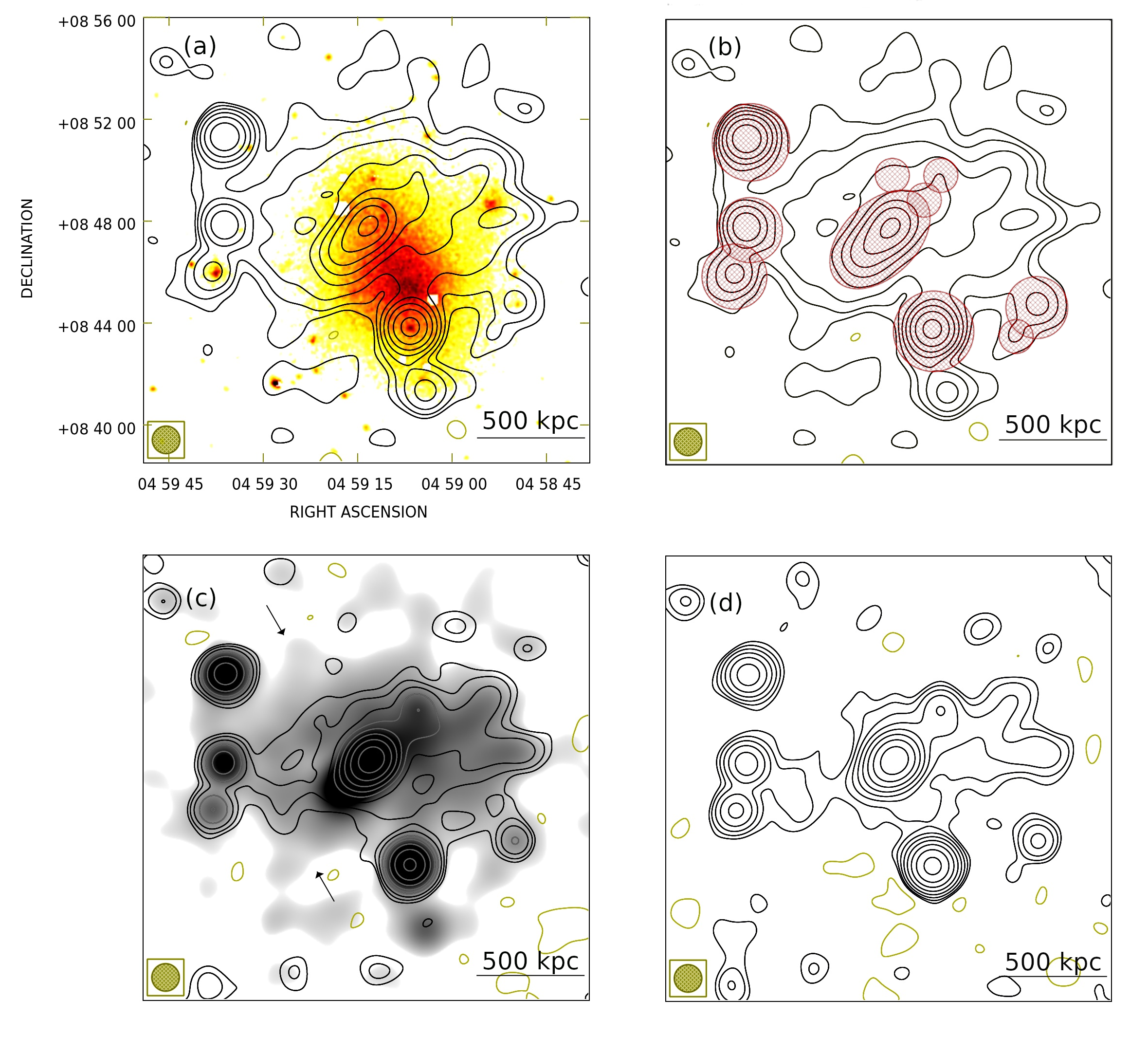
Figure 3: Panel (a): Radio emission in black contours from the galaxy cluster A523 at 144 MHz ($\sigma=1.3$ mJy/beam) overlaid on the X-ray image of the cluster from XMM-Newton (Cova et al., 2019) in colors, see the text for more details. Panel (b): Contours are the same as in panel (a), with regions used to mask the emission of discrete sources shown in red. Panel (c): Radio emission in black contours from the galaxy cluster A523 at 1.410 GHz ($\sigma=0.14$ mJy/beam) overlaid on the radio emission in gray colors at 144 MHz. Arrows point to the regions in the north-east and south-east detected with LOFAR but not with the VLA. Panel (d): Radio emission in black contours from the galaxy cluster A523 at 1.782 GHz ($\sigma=0.11$ mJy/beam). All radio images are shown at 65^′′ of resolution and the synthesised beam is shown in the bottom left. Black contours start at 3$\sigma$ and scale by a factor 2, while negative 3$\sigma$ contours are drawn in army green. In each panel the horizontal black bar corresponds to 500 kpc at the chosen cosmology.

In Fig. 2 we show the radio image of the cluster at 144 MHz obtained with LOFAR at 20^′′. The radio image is superimposed on the background-subtracted and exposure-corrected XMM-Newton image, with point sources removed. The X-ray image has been obtained with the combination of data from the three EPIC instruments in the soft 0.5-2.5 keV band for a total exposure time of about 220 ks and was recently published by Cova et al. (2019). Dashed and dotted lines indicate respectively the primary (SSW-NNE) and secondary (ESE-WNW) merger axis. The diffuse radio source extends further than filaments F1 and F2, and a third filament, F3, is visible, with a size of $7^{\prime}\,\times\,1^{\prime}$ (i.e., 830 kpc $\times$ 120 kpc), that embraces S5 and terminates near the roundish patch of emission P. Overall, the diffuse emission sits in the northern part of the thermal gas distribution, is characterized by an E-W linear morphology that is approximately perpendicular to the axis of the main merger in the SSW-NNE direction, cuts through the central part of the X-ray region, and encompasses the discrete sources S1, S2, S3, S4, and S5 (see Fig. 2).

Flux density of point sources

In Table 3, we report the position and flux densities of the discrete sources S1-S10 at 144 MHz, 1.410 GHz, and 1.782 GHz estimated from the images at 13.5^′′, obtained by applying the same uv-range and weighting-scheme (robust=-1) at the three frequencies. As in Vacca et al. (2018b), we model the sources with a 2-dimensional elliptical Gaussian sitting on a plane. Overall, there are nine free parameters of the fit: the x, y coordinates in the sky of the centre of the Gaussian, the full width half maximum along the two axes, the position angle, the amplitude, and the three components of the direction normal to the plane. The non-zero baseline fit ensures that any contribution from the diffuse emission, if present, is not absorbed into the flux density of the sources. The uncertainty has been estimated by adding in quadrature the uncertainty derived from the fit procedure and the flux scale uncertainty at the corresponding frequency (20% at 144 MHz and of 2.5% at 1.410 and 1.782 GHz). This procedure was used for all the discrete sources except the central AGN S1. Being an extended source, we determined the flux density by applying a 3$\sigma$ sensitivity threshold to the LOFAR image ($\sigma=0.5$ mJy/beam) and blanked the two VLA images in the same regions as the LOFAR one. We refer to § 5.3 for spectral studies of these sources.

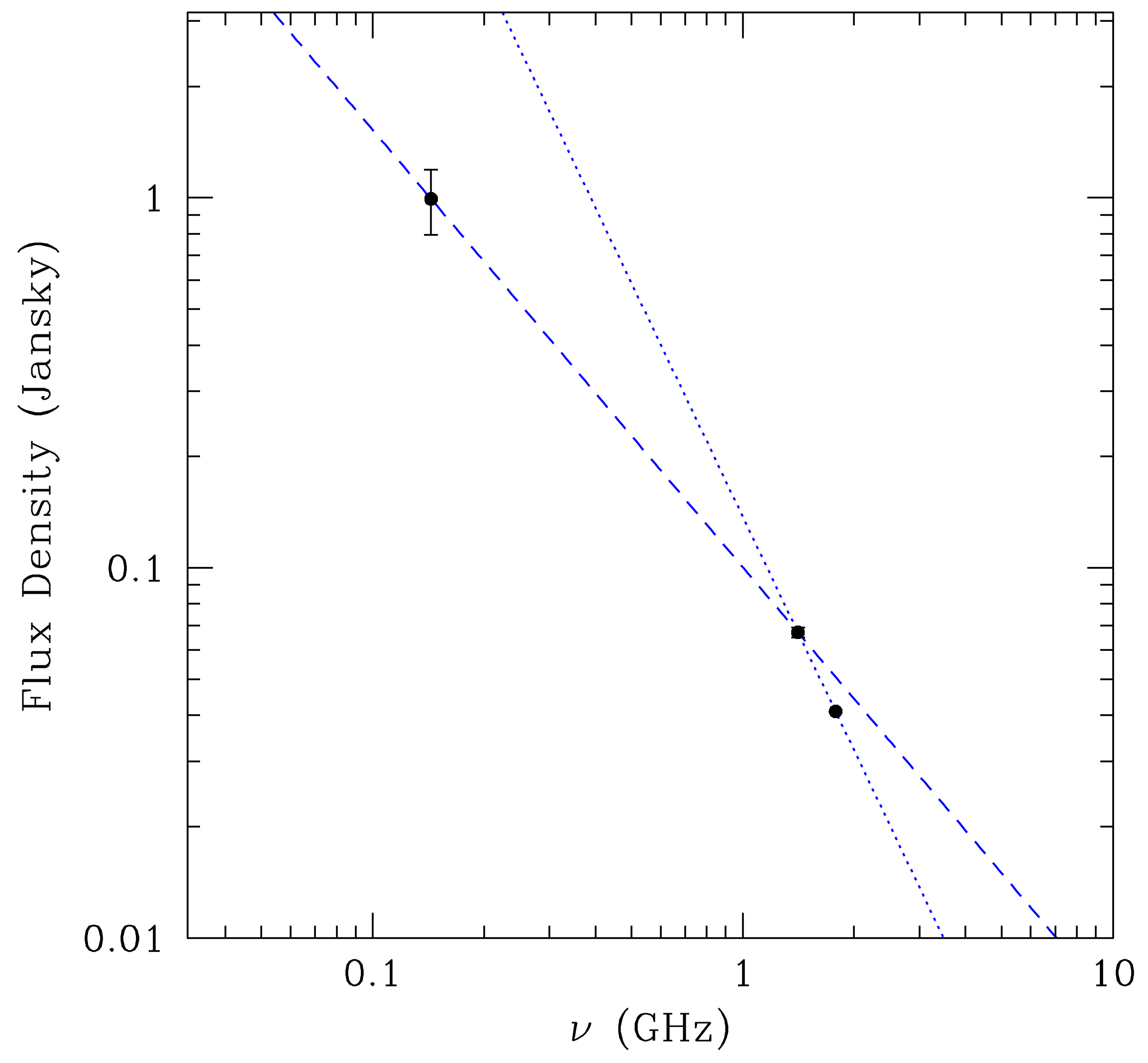
Figure 4: Flux density of the diffuse emission in A523 versus frequency. The power-law fit of the 144 MHz and 1.410 GHz data points is shown in dashed blue, while the fit of the 1.410 GHz and 1.782 GHz data points in dotted blue.

Table 4: Details of the spectral index maps. Col. 1, 2: minimum and maximum cut in uv-range; Col. 3, 4: minimum and maximum angular scales accessible with the data; Col. 5: original resolution of the 144 MHz image; Col. 6: original resolution of the 1.410 GHz image; Col. 7: restored beam.

uv-min	uv-max	$\theta_{\rm min}$	$\theta_{\rm max}$	Beam${}_{\rm 144\,MHz}$	Beam${}_{\rm 1.410\,GHz}$	Beamrestored
$\lambda$	$\lambda$	$\prime\prime$	$\prime$	${\prime\prime}\times{\prime\prime}$	${\prime\prime}\times{\prime\prime}$	${\prime\prime}\times{\prime\prime}$
158	4835	48	22	$34.5\times 46.6$	$36.1\times 49.8$	$65\times 65$
158	16980	14	22	$7.8\times 15.9$	$13.0\times 16.3$	$20\times 20$

Flux density of diffuse emission

In panel (a) of Fig. 3 we show in black contours the LOFAR image of the cluster at 144 MHz overlaid on the same X-ray image as in Fig. 2, while in panel (b) the LOFAR image with the regions used to mask discrete sources. In the panels (c) and (d), we show on the left the new VLA image at 1.410 GHz in contours overlaid on the LOFAR image in gray scale and on the right the new VLA image at 1.782 GHz. All the radio images are at 65^′′ resolution. Comparison of the LOFAR and VLA images shows that the radio halo appears more extended at lower frequencies. The LOFAR image at 65^′′ indeed reveals a size of the source of about 15^′, corresponding to 1.8 Mpc at the cluster distance. The maximum angular scale accessible with our data is about 1.2^∘, 22^′, and 17^′ respectively at 144 MHz, 1.410 GHz and 1.782 GHz, as reported in Table 2. The sensitivities $\sigma$ at these three frequencies and spatial resolution are 1.3 mJy/beam, 0.14 mJy/beam, and 0.11 mJy/beam. A brightness of 3.9 mJy/beam at 144 MHz (i.e., at 3$\sigma$), as the faintest regions of the emission in the LOFAR image, corresponds to 0.400-0.160 mJy/beam at 1.410 GHz and to 0.315-0.115 mJy/beam at 1.782 GHz, for typical spectral index values ($\alpha=1-1.4$). A sensitivity $\sigma$ of 0.133-0.053 mJy/beam at 1.410 GHz and of 0.105-0.038 mJy/beam at 1.782 GHz is needed to detect this emission, while the sensitivity in our images is 0.14 mJy/beam and 0.11 mJy/beam respectively at 1.410 GHz and 1.782 GHz, see Table 2. The larger extent detected at LOFAR frequencies compared to VLA higher frequency images is therefore likely due to the better sensitivity to steep spectrum emission of LOFAR.

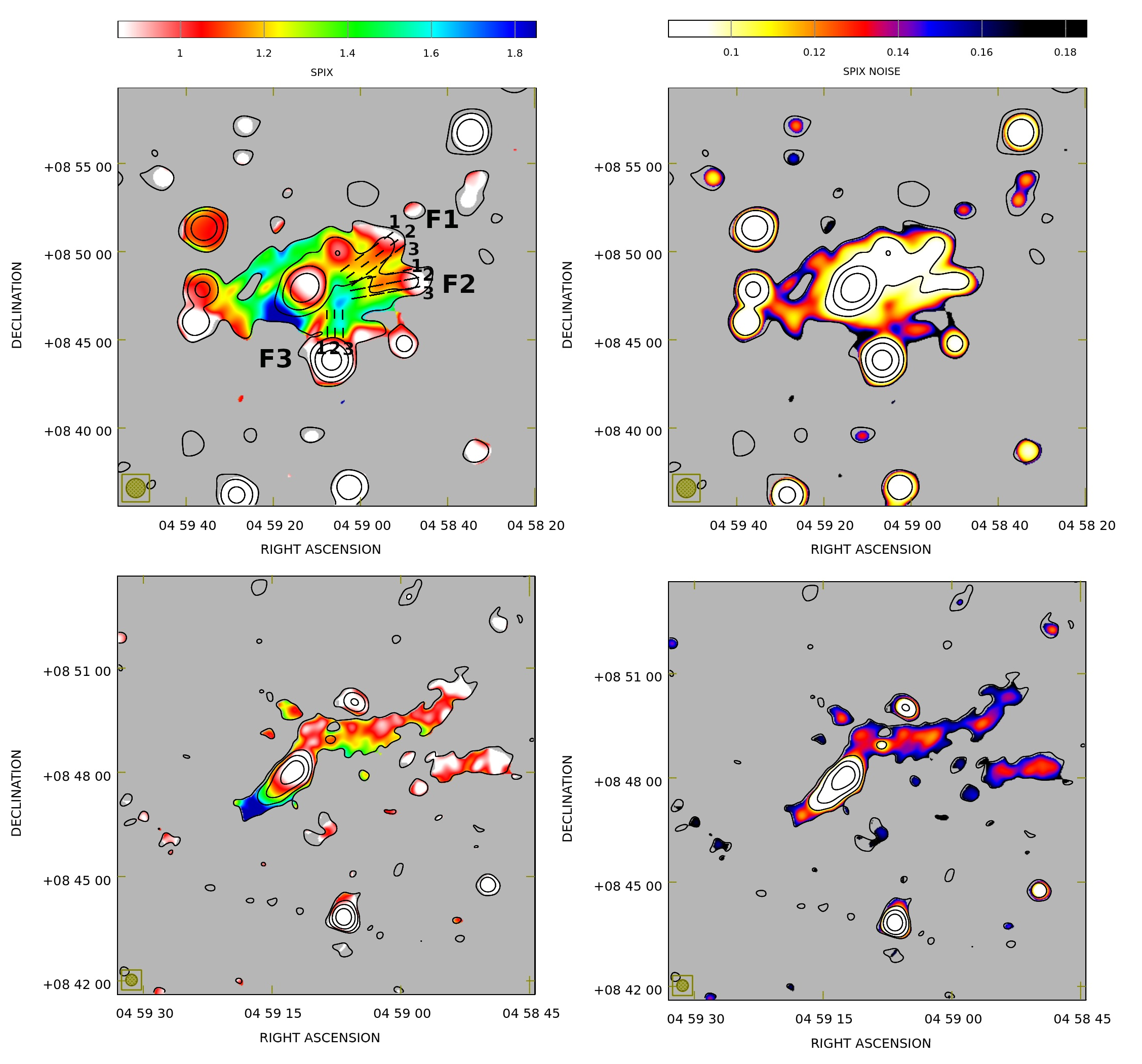
Figure 5: Top panels: Spectral index (left) and spectral index uncertainty (right) image of A523 between 144 MHz and 1.410 GHz at 65^′′ resolution. Contours represent the radio emission at 1.410 GHz at the same spatial resolution, start at 3$\sigma$ and increase by a factor 4 ($\sigma=0.13$ mJy/beam). Bottom panels: Spectral index (left) and spectral index uncertainty (right) image of the central region of A523 between 144 MHz and 1.410 GHz at 20^′′ resolution. Contours represent the radio emission at 1.410 GHz at the same spatial resolution, start at 3$\sigma$ and increase by a factor 4 ($\sigma=75\,\mu$Jy/beam).

A faint region of diffuse emission in the north-east and in the south of the cluster emerges in the 144 MHz image at 65^′′, along the main merger axis (see arrows in Fig. 3), panel (c), along the optical and X-ray distribution of the system, see Fig. 1 in Girardi et al. (2016). Consequently, at this frequency the emission along the SSW-NNE axis is more prominent than at $\sim$1-2 GHz. At 1.410 GHz only the brightest regions along the ESE-WNW direction survive, while the emission in the south, in the south-east and in the north-east falls below the noise. At 1.782 GHz, the diffuse emission dims further, the filaments F1, F2, part of F3 and a bridge of radio emission connecting S1 to S6 only are still apparent. In order to measure the flux densities at the three frequencies, we masked embedded compact sources as shown in Fig. 3 (panel b). We assume that the halo extends over the location of embedded compact sources. In these masked regions we assume the halo radio brightness is equal to its mean radio brightness over the entire unmasked diffuse source. Overall, we derive a flux density at 144 MHz of $S_{\rm 144\,MHz}\,=\,(1.52\,\pm\,0.31)$ Jy, including the southern patch. The uncertainty takes into account the uncertainty on the flux scale and the image noise. By using the same method to extrapolate over embedded masked regions, at 1.410 GHz we measure a flux density of the diffuse emission of $S_{\rm 1.410\,GHz}\,=\,(70\,\pm\,2)$ mJy, in agreement within $\approx$ 0.8$\sigma$ with the flux density derived by Girardi et al. (2016) $S_{\rm 1.4\,GHz}\,=\,(72\,\pm\,3)$ mJy, while at 1.782 GHz we measure a flux density $S_{\rm 1.782\,GHz}\,=\,(42\,\pm\,1)$ mJy. These flux densities have been derived considering all the available uv-range and applying a sensitivity cut of 3$\sigma$ at the corresponding frequency, so they refer to the full size of the source at those frequencies.

In panel (a) of Fig. 3, the patch P is more extended compared to Fig. 2 and blended with S5 and with the rest of the diffuse emission. In order to better discriminate the emission associated with this source, we used the 20^′′ image. We measure a flux density $S_{\rm 144\,MHz}\,=\,(49\,\pm\,10)$ mJy and an average brightness $4.5\,$mJy/beam. While this patch is clearly detected at 144 MHz, only an excess is present at the $3\sigma$ level ($\approx\,0.4$ mJy/beam) at 1.410 GHz, suggesting a spectral index $\alpha\gtrsim 1.5$. The origin of this emission will be discussed in §5.1.

5 Spectral index

In Fig. 4 we plot the flux density of the diffuse emission at 144 MHz, 1.410 GHz, and 1.782 GHz versus frequency, derived from images obtained by selecting the same uv-range (196-4835$\lambda$), weighting-scheme (robust=-0.5), and area on the sky. The $uv_{\rm min}=196\lambda$ is imposed by the minimum uv-sampling at 1.782 GHz. The corresponding images at 144 MHz, 1.410 GHz, and 1.782 GHz are not shown here. Overall, the spectrum cannot be described with a single power-law, since it steepens towards high frequency. Indeed, as discussed in § 4, at 1.782 GHz only the filaments F1, F2, part of F3, and a bridge connecting S1 to S6 survive, the rest of the emission is buried by the noise. We fit the spectrum with the software synage (Murgia, 1996) assuming a power-law. Between 144 MHz and 1.410 GHz we obtain $\alpha_{\rm 144\,MHz-1.410\,GHz}=1.2_{-0.2}^{+0.1}$ (see dashed line in Fig. 4), while between 1.410 GHz and 1.782 GHz we obtain $\alpha_{\rm 1.410\,GHz-1.782\,GHz}=2.1_{-0.3}^{+0.2}$ (see dotted line in Fig. 4). A similar behaviour has been observed for other radio halos (e.g., Deiss et al., 1997; Thierbach et al., 2003; Xie et al., 2020; Rajpurohit et al., 2021b). However, our frequency range is smaller than in these studies, where it extends up to about 5 GHz.

In order to perform a detailed analysis of the spectral index properties of the diffuse emission, we produced spectral index images at low- and high-spatial resolution with our new LOFAR observations at 144 MHz and the VLA data at 1.410 GHz presented in § 3. We selected the same uv-range and weighting-scheme (robust=-0.5) at the two frequencies both at high and at low spatial resolution and a beam of $65^{\prime\prime}$ and 20^′′ was restored, respectively, in the two cases. All the details about the selected uv-range, the corresponding angular scales accessible through the data, the original spatial resolution of the images and the size of restored beams are reported in Table 4. All the images have been regridded to a common frame in order to have the same pixel size.

The spectral index maps have been obtained by applying a sensitivity cut in radio brightness of 3$\sigma$ at both frequencies simultaneously, in order to exclude pixels that are below 3$\sigma$ in at least one of the two images. Flat-spectrum regions above the noise level at 1.410 GHz but not at 144 MHz and steep-spectrum regions detected at 144 MHz but not at 1.410 GHz will be missed with this procedure. In particular, the peripheral regions that are detected at 144 MHz but not at 1.410 GHz are characterized by a spectral index steeper than $\alpha\gtrsim 0.9$. In order to investigate the spectral index behaviour also in these regions, we directly compare the brightness profile at 144 MHz and 1.410 GHz without applying any sensitivity cut to the images.

5.1 Spectral index images

The spectral index distribution (left) and its uncertainty (right) are shown in Fig. 5 at both low (65^′′, top panels) and high (20^′′, bottom panels) spatial resolution. The spectral index trends observed at low resolution are consistent with those observed at higher spatial resolution. However, at 20^′′ resolution, only the brightest parts of the emission are visible.

The low-resolution spectral index image between 144 MHz and 1.410 GHz reveals a patchy distribution with a flattening in the west at the location of the filaments, and a steepening both in the north-east and in the south-east. In particular, the region in the south-east of S1 is characterized by a spectral index $\alpha\sim 1.2-2.2$, likely because it is contaminated at least in part by the steep spectrum tails of S1. The north-east and south of the diffuse emission appear well detected in the 144 MHz image but fall below the noise at 1.410 GHz, with the brightest patches at 144 MHz reaching radio brightness up to 20 mJy/beam. If we take a brightness upper limit of 0.39 mJy/beam at 1.410 GHz (i.e., 3$\sigma$ with $\sigma=0.13$ mJy/beam), we derive a spectral index $\alpha>1.7$.

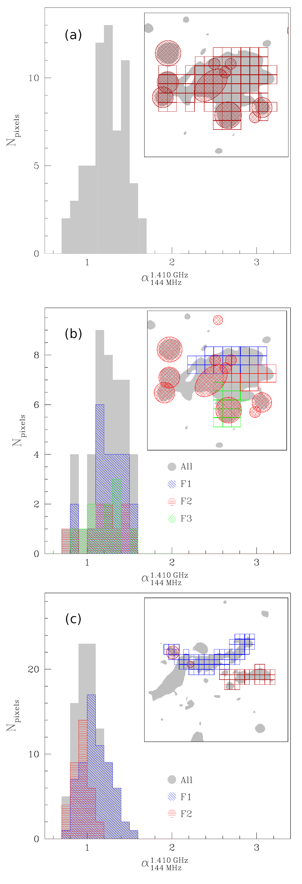
Figure 6: Panel (a): Histogram of the low-resolution spectral index image obtained covering the image with the grid shown in the inset and masking discrete sources. Panel (b): Histogram of the spectral index values at the location of the filaments at 65^′′ (overall in gray, F1 only in blue, F2 only in red, and F3 only in green). Panel (c): Histogram of the spectral index values at the location of the filaments at 20^′′ (overall in gray, F1 only in blue, and F2 only in red). In all cases the side of the cells of the grid has a size equal to the beam FWHM.

Table 5: Spectral index values for the full diffuse emission, the filaments and along each filament. Col. 1: Region considered for the average; Col. 2, 3, 4: average spectral index $\langle\alpha\rangle$, its dispersion $\sigma_{\alpha}$ and the average uncertainty $\langle\sigma_{\alpha}\rangle$; Col. 5: spatial resolution of the images used for the measurements.

Source	$\langle\alpha\rangle$	$\sigma_{\alpha}$	$\langle\sigma_{\alpha}\rangle$	Beam ($\prime\prime$)
All	1.2	0.2	0.1	65
Filaments	1.2	0.2	0.1	65
F1	1.3	0.2	0.1	65
F2	1.2	0.3	0.1	65
F3	1.2	0.2	0.1	65
Filaments	1.0	0.2	0.1	20
F1	1.1	0.2	0.1	20
F2	0.9	0.1	0.2	20

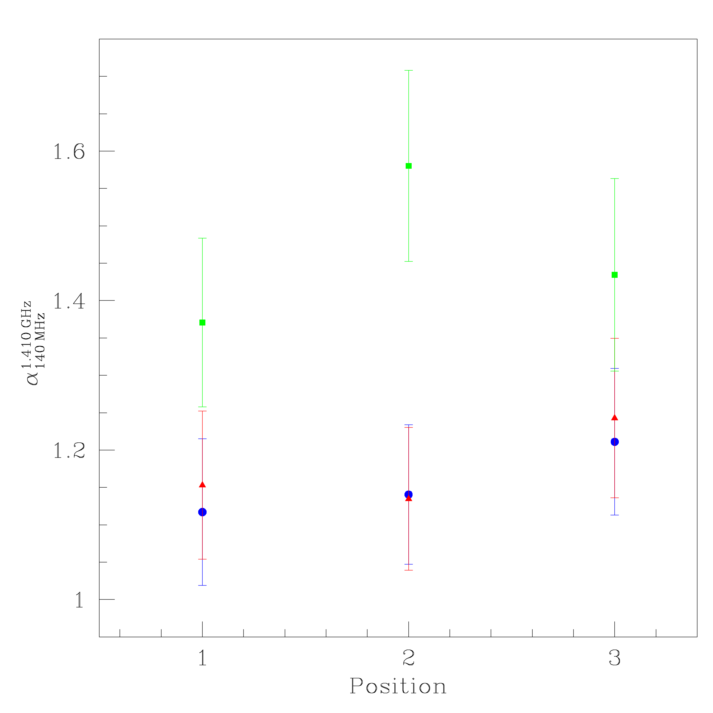
Figure 7: Spectral index along filament F1 (blue dots), filament F2 (red triangles) and filament F3 (green squares). The slices are shown in the top left panel of Fig. 5 and the numbers on the x-axis indicate the slice identification number as reported in the same figure, see the text for more details.

In Fig. 6 (panel (a)) we show the histogram of the spectral index values of the diffuse emission obtained covering the low resolution spectral index image with a grid, after masking compact sources, as shown in the inset. The side of the cells is equal to the full width at half maximum (FWHM) of the beam. We derive an average spectral index $\langle\alpha\rangle=1.2$, a dispersion $\sigma_{\alpha}=0.2$, and an average value of the spectral index statistical uncertainty $\langle\sigma_{\alpha}\rangle=0.1$, see Table 5. The average spectral index statistical uncertainty has been derived from the spectral index uncertainty image (top right panel in Fig. 5). This image has been obtained by evaluating the statistical uncertainty on a pixel basis, including both the flux density scale uncertainty and the thermal noise of the two radio images. If the patchy structure of the spectral index image is due to measurement uncertainties, we expect that the mean value of the uncertainty image and the dispersion of the spectral index distribution are consistent. The dispersion is only slightly higher than the uncertainty derived by using the spectral index noise image suggesting that, even if some degree of intrinsic complexity is present, the observed fluctuations are dominated by the measurement uncertainties. Following Orrú et al. (2007), since the total dispersion is the result of the sum in quadrature of the uncertainty and of the intrinsic scatter

$$\sigma_{\alpha}=\sqrt{\langle\sigma_{\alpha}\rangle^{2}+\sigma_{\rm int,proj}^{2}},$$ (1)

we derive an intrinsic scatter in the spectral index $\sigma_{\rm int,proj}=0.17$ projected in the plane of the sky on scales of the beam, i.e. 65^′′. If the spectral index varies stochastically along the line of sight over the full diffuse emission region, we derive a 3-dimensional intrinsic spectral index $\sigma_{\rm int}=\sqrt{N}\sigma_{\rm int,proj}=0.67$, where $N=15$ is the number of cells assuming that the maximum size of the source along the line of sight is similar to the largest linear size in the plane of the sky, i.e., 15^′. This is comparable to the value derived by Botteon et al. (2020) for the emission in A2255 and higher than the value derived for the radio halos in the Toothbrush cluster by van Weeren et al. (2016b) and in A520 by Hoang et al. (2019) by a factor of $\sim 7$ and 2 respectively.

Filaments

In the west of the source, the spectral index distribution shows a flattening at the location of the three filaments. Histograms of the spectral index distribution in this region are shown in the panels (b) and (c) of Fig. 6. In the central panel, we show the statistics derived from the low-resolution image, using the LOFAR image at 20^′′ to determine the location and size of the filaments. Considering all the filaments simultaneously, the average spectral index is $\langle\alpha\rangle=1.2\pm 0.1$. When considered separately, we derive respectively $\langle\alpha\rangle_{\rm F1}=1.3\pm 0.1$, $\langle\alpha\rangle_{\rm F2}=1.2\pm 0.1$, and $\langle\alpha\rangle_{\rm F3}=1.2\pm 0.1$, see Table 5. However, the low resolution image hinders a detailed analysis of the spectral properties of the filaments, due to a blending with the rest of the diffuse emission. In the panel (c) of Fig. 6, we show the histograms of the spectral index distribution along the filaments obtained from the high-resolution image. We carried out our measurements only for F1, still clearly visible, and for the brightest region of F2. Only a small patch of F3 survives, therefore we did not include it in the analysis. We find an overall average spectral index $\langle\alpha\rangle=1.0\pm 0.1$, and $\langle\alpha\rangle_{\rm F1}=1.1\pm 0.1$ and $\langle\alpha\rangle_{\rm F2}=0.9\pm 0.2$, respectively for F1 and F2, see Table 5. Even if still in agreement within the measurement uncertainties, the spectral index in the brightest regions of these filaments appears slightly flatter than the rest of the source, and in particular, the emission along the filaments F2 is characterized by a flatter spectrum than that along F1. However, this difference could be due to the fact that in the high resolution image we are only probing the brightest regions of F2, while for F1 more structure is used.

A qualitative inspection of the 65^′′ image indicates that moving away from the filament brightest region, the spectral index becomes steeper. To quantify this behaviour, we computed the spectral index along slices in the low-resolution image. For each filament we used three slices: a central one located along the brightest part of the filament and two others, one on each side. Slices are one pixel in width, spaced by half FWHM (i.e., 32.5^′′) and with lengths comparable to the length of the filaments. To better identify the filaments we used the high resolution LOFAR image at 20^′′. In Fig. 7, we show the average spectral index along the three slices for the three filaments: filament F1 in blue dots, filament F2 in red triangles and filament F3 in green boxes. The location of the slices is shown in Fig. 5 and is identified with the numbers 1, 2, and 3 (numbered from North to South for F1 and F2 and from left to right for F3), as reported in the x-axis of Fig. 7. F1 shows a spectral index decreasing from south to north, while F2 shows a spectral index slightly steeper moving towards both north and south. However, within the errors, the two filaments show similar spectral indices with variations between 1 and 1.3. Finally, F3 has a steeper spectral index that varies in the range 1.3-1.7 with increasing values at the location of the brightest patches of the emission. The different spectral behaviour of F1 and F2 with respect to the surrounding medium could be related to a stronger magnetic field that allows us to detect lower-energy electrons with a flatter spectrum. Spectral index images of these filaments at higher resolution are necessary to investigate in more depth their behaviour, with no contamination from the rest of the diffuse emission.

Filaments of diffuse emission have also been observed in the galaxy cluster A2255. Govoni et al. (2005) classified them as peripheral structures associated with the radio halo in agreement with expectations from numerical simulations (Loi et al., 2019), while Pizzo et al. (2011) classified them as relics, due to their morphology, fractional polarization level and rotation measure. The filaments in A2255 show spectral indices flatter ($\alpha\sim 0.8-1.3$) than the rest of the diffuse emission (up to $\alpha\sim 2$), see also Botteon et al. (2020). Similar filamentary emission has been recently identified in the diffuse emission in MACS J0717.5+3745 characterized by a spectral index of $\alpha\sim 1.2$ (Rajpurohit et al., 2021a). Rajpurohit et al. (2021b) speculate that such features may be due to the complex distributions of shocks caused by the merger in the cluster. In line with this, the filaments in A523 could be either radio relics or associated with the peripheral regions of the radio halo. Discriminating between the two is not a trivial task. F1 and F2 could be associated with shock waves produced by the main merger along the SSW-NNE direction, while F3 could be associated with a shock wave produced by the secondary merger along the perpendicular axis. Shock fronts have not been detected at the sensitivity of X-ray observations currently available and, only in case of the filament F1, the morphology and the spectral index distribution could support this possibility. In the case of a merger with some inclination with respect to the plane of the sky, the detection of shock waves and of a spectral gradient could be hindered by projection effects. The available X-ray and optical data do not show evidence of a merger component along the line of sight. Such a component could be possibly associated with the secondary merger. However, at the moment, no indication of this emerges from the data. For a detailed description of the sub-clumps and of the merger geometry see Girardi et al. (2016) and Cova et al. (2019).

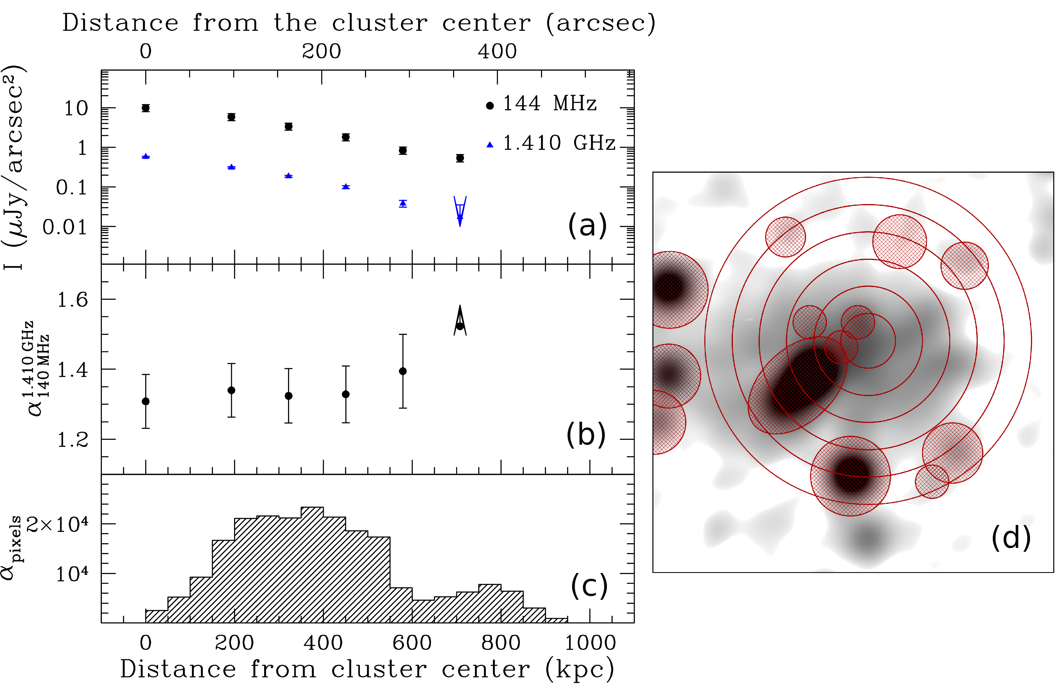
Figure 8: Panel (a): Radial profile of the radio brightness at 144 MHz (black dots) and 1.410 GHz (blue triangles) with respect to the radio peak, using the annuli shown in the panel (d). Panel (b): Radial profile of the spectral index of the diffuse emission obtained from the radio brightness profiles in the panel (a). Panel (c): pixel distribution of the spectral index 65^′′ image as a function of the distance from the radio peak at 144 MHz. The pixel distribution does not depend on the annuli chosen to produce the radial profiles shown in the above panels. Panel (d): Gray scale shows the LOFAR image at 144 MHz at 65^′′, as well as annuli with a beam-size width centered on the radio peak at 144 MHz and used in order to derive the radial profile. Discrete sources have been masked and therefore not included in the measurements.

Patch P

Patch P is clearly detected at 144 MHz at about RA ${\rm 04h:59m:04s}$ and Dec ${\rm+08^{\circ}:41^{\prime}:23^{\prime\prime}}$, while only the peak of the emission associated with it is visible at 1.410 GHz, with a brightness of $\approx$ 0.4 mJy/beam. If we compare this value with the peak radio brightness at 144 MHz, i.e. $42\,$mJy/beam, we obtain a spectral index $\alpha=2.0$ in the brightest region of the emission. This steep value might suggest that the patch P could be a very old object, relic emission from a radio lobe, or plasma emitted by a now-quiescent AGN. The closest radio galaxy is the source S5 (z=0.1041, Girardi et al., 2016) which shows signs of possible re-starting jets when inspected at high spatial resolution (see Fig. 1). Patch P is distant almost $\sim 2.5^{\prime}$ from S5, corresponding to a projected linear distance of about 300 kpc. If patch P is a remnant lobe of previous activity of S5, it could have moved up to the distance where we observe it now. In this case, its linear size would be about 170 kpc. Alternatively, if we select close optical sources from Girardi et al. (2016) and Golovich et al. (2019) within a radial distance of one beam (65^′′) from the peak of patch P, we find 18 sources with redshift 0.097$\lesssim z\lesssim$0.637, translating into a linear size of the source between 170 kpc and 640 kpc, the closest being a source at z$\approx$0.637. According to radiative cooling models, old remnant sources are expected to be characterized by very steep spectra ($\alpha\gtrsim 1.2$, Pacholczyk, 1970) and observations of the Lockman Hole field with LOFAR show that these sources represent a few percent of the low resolution catalogue of radio sources in this field (Brienza et al., 2017).

A second possibility is that this source is the continuation of the radio filament F3 or a diffuse synchrotron emission associated with an high-redshift galaxy cluster, since the closest galaxy in projection is the galaxy at z=0.637 detected at $\approx$11^′′ from the source radio peak. In the latter case the radio largest linear size of the source would be about 570 kpc, its radio power at 144 MHz $\sim 1.7\times 10^{26}$ W/Hz and at 1.410 GHz $\sim 1.8\times 10^{24}$ W/Hz, still consistent with typical radio powers observed for radio halos (see Giovannini et al. 2009, Feretti et al. 2012 and van Weeren et al. 2019). Assuming the scaling relation $P_{\rm 150\,MHz}$-$M_{\rm SZ,500}$, $P_{\rm 1.4\,GHz}$-$M_{\rm X,500}$, and $P_{\rm 1.4\,GHz}$-$L_{\rm X,0.1-2.4\,keV}$ (van Weeren et al., 2021; Yuan et al., 2015), we predict a mass of the system $M_{\rm 500}$ in the range $8-11\times 10^{14}M_{\odot}$ and an X-ray luminosity $L_{\rm X,0.1-2.4\,keV}=4-18\times 10^{44}\,M_{\odot}$. These values are consistent with those observed for galaxy clusters at similar redshift (e.g., Schneider, 2015). However, we note that such a system would be very massive and therefore very rare.

Finally, a third possibility is that this source is an Odd Radio Circle (ORC, Norris et al., 2021). The size, morphology and spectral properties resemble those of this new class of sources discovered with Australian Square Kilometre Array Pathfinder (ASKAP). The known ORCs have been observed in the direction of high-redshift galaxies and, interestingly, close to the location of patch P one galaxy is detected at z=0.637. However, these objects show a bright limb not observed here and the galactic latitude of patch P is lower than that observed for ORCs. If confirmed, this would be the first ORC seen by LOFAR.

5.2 Spectral index profile

In Fig. 8, the radial profiles of the radio brightness at 144 MHz (black dots) and 1.410 GHz (blue triangles) are shown in panel (a), while the corresponding spectral index profile is shown in panel (b). These profiles are derived by using concentric annuli centered on the radio peak at 144 MHz on the same 65^′′ radio brightness images used to derive the spectral index spatial distribution. The annuli have widths of one beam size. The statistics are evaluated after masking all the embedded discrete sources as shown in the right panel, including S1, whose steep tails could otherwise contaminate our estimation. A few additional sources have been masked with respect to those labeled in Fig. 1 because they are characterized by a radio brightness peak $\gtrsim\,8\,\sigma$ at 1.410 GHz.

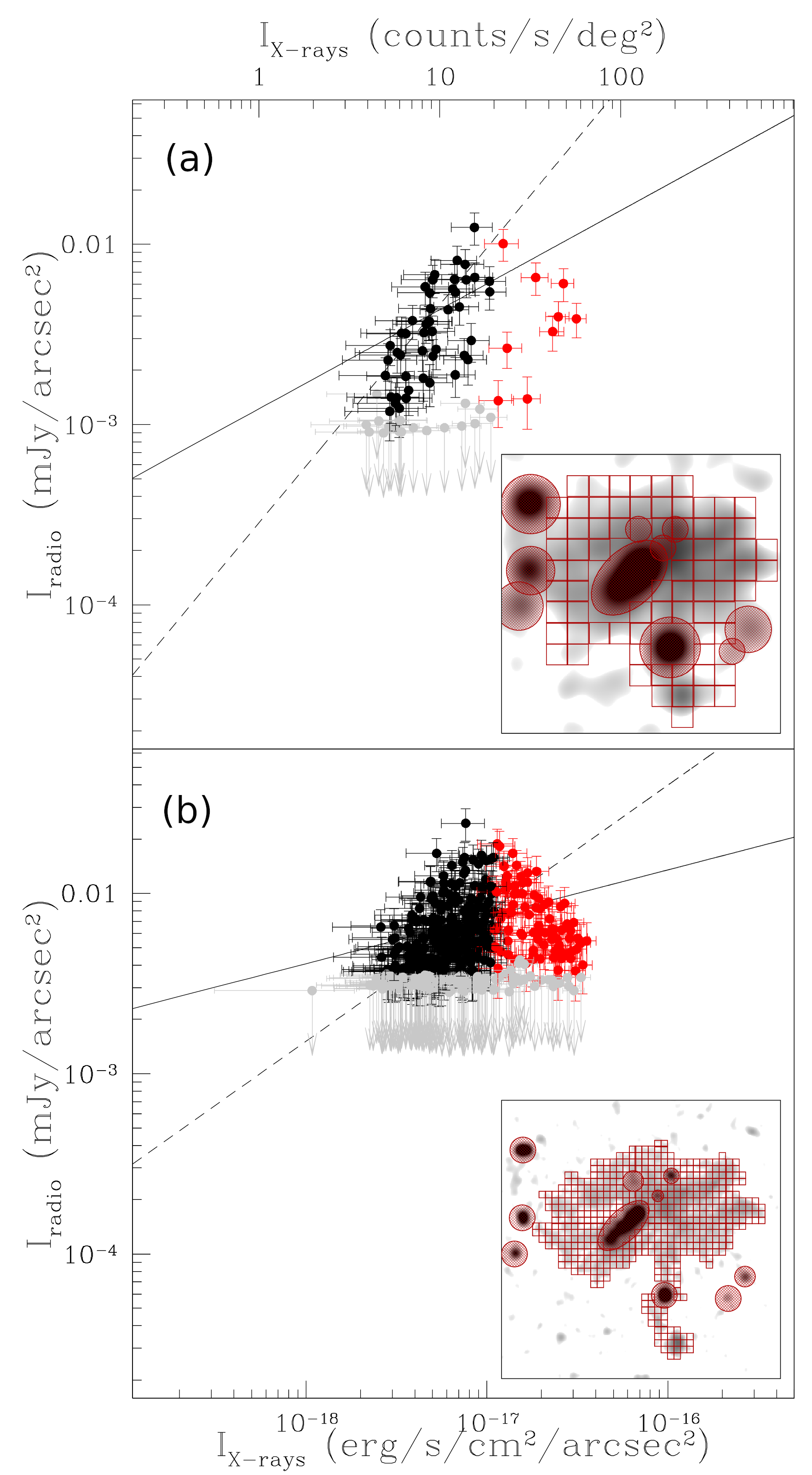
Figure 9: Radio 144 MHz versus X-ray surface brightness of the cluster at 65^′′ (panel (a)) and at 20^′′ (panel (b)): upper limits of the radio emission in gray, points corresponding to X-ray emission larger than 20 counts/s/deg² in red and smaller than 20 counts/s/deg² in black. The continuous line represents the power-law fit including all data points, while the dashed line represents the fit only considering points corresponding to an X-ray emission lower than 20 counts/s/deg² (including upper limits). The inset panels show the grid on the radio emission of the cluster at 144 MHz.

Panel (c) in Fig. 8 shows the pixel distribution of the spectral index image at 65^′′ (top left panel in Fig. 5), as a function of the distance from the radio peak at 144 MHz, after masking embedded discrete sources. The pixel distribution indicates that the low-resolution image only properly samples regions out to 500-600 kpc due to the sensitivity cut we applied. In this region, the radial profile provides an average spectral index $\alpha\sim 1.2$, in agreement within the uncertainty with the mean over the spectral index image, see § 5.1. Since we do not apply any sensitivity cut to derive the spectral index radial profile, the radial profile can give us some indication about the spectral index behaviour also beyond 600 kpc, in regions where the radio brightness is below the 3$\sigma$ level. In this way, possible flattening and/or steepening in the spectral index distribution can be possibly detected. Beyond 600 kpc, we derive a lower limit of the spectral index of $\alpha\,\gtrsim\,$1.5. Results in regions covered by the most external annulus must be interpreted with caution. Indeed, the emission here is below the noise level of an individual beam and, as we used a deconvolution threshold of 1$\sigma$ and therefore signal below this threshold it is not deconvolved, LOFAR emission may result in a brighter signal than reality, leading to artificial spectral steepening. Moreover, we note that even though we match VLA and LOFAR uv-range, the density of the points in the inner of the uv-plane is much higher in LOFAR than in the VLA data. However, the impact of this on the images is very difficult to estimate. The diffuse emission in A523 does not show a circular shape and the radio and X-ray emission do not fully overlap. A substantial offset between the peak in X-ray surface brightness and radio brightness is also present at 144 MHz, the largest absolute offset observed for radio halos and among the largest fractional offsets (offset/size) when giant radio halos only are considered (Feretti et al., 2012), as expected in case of a magnetic field fluctuating on large spatial scales (e.g., Vacca et al., 2010). This offset makes the radial profile of the spectral index and its link with the thermal properties of the system difficult to interpret. No steepening is observed even when the spectral index is computed as a function of the distance from the peak in the X-ray emission (not shown here).

5.3 Spectral index of discrete sources

The presence of the radio galaxies identified in § 4 is apparent in the spectral index images shown in Fig. 5. Flux densities of these sources have been derived as described in § 4. Spectral index values between 144 MHz 1.410 GHz are given in Table 3. For the sake of comparison, we report in Table 3 the flux density and spectral index values by de Gasperin et al. (2018), derived by using observations at 147 MHz from the TIFR GMRT Sky Survey (TGSS, Intema et al., 2017) and at 1.4 GHz from the NVSS (Condon et al., 1998). The sources in the catalog have been identified by imposing a distance in RA and Dec respectively of $\lesssim 25^{\prime\prime}$ from our sources, comparable to the TGSS spatial resolution. TGSS flux densities are available for four out of ten sources and the NVSS flux densities for six of them. The remaining sources are probably too faint to be detected at the corresponding sensitivity of TGSS and/or NVSS. The NVSS fux density of the sources agrees with our VLA values within at most 1.3$\sigma$, while the TGSS measurements agree with our LOFAR flux densities within at most 1.9$\sigma$, with LOFAR measurements being systematically slightly higher, . This is likely due to a difference in the flux density scale of our LOFAR observations with respect to the TGSS data that, comparing the flux densities of these four sources, amounts to a factor of about $1.4-1.6$. Position-dependent flux density scale variations have been found in the TGSS by other authors (Hurley-Walker, 2017). The de Gasperin et al. (2018) catalog reports spectral index information for six of our sources (S1, S5, S6, S7, S8, and S9, Col. 10, Table 3), derived from the TGSS and NVSS flux density values. However, for two of them (S6 and S9), the TGSS flux density given in the catalog is zero (see Col. 6, Table 3), therefore it is unclear how the spectral index has been derived and we will neglect them in the following. The spectral indices of the remaining four sources differ with respect to our by about 2.3$\sigma$ for S1, 1.7$\sigma$ for S5, 0.4 $\sigma$ for S7, and 1.5$\sigma$ for S8 (for each source $\sigma$ has been computed with the same approach described in Footnote 9). Our flux density measurements for S1 include the contribution from the diffuse emission. Given the size of the source and the mean radio brightness of the overall diffuse emission, this term amounts to about 35 mJy and 2 mJy respectively at 144 MHz and 1.4 GHz. However, as per our knowledge, the flux densities given in the public catalog include this contribution as well and therefore the difference in the flux densities and in the spectral indices can not be ascribed to it. Our spectral index for source S1 is flatter than the published value, likely also because of the slightly higher flux density measured from the NVSS with respect to our VLA measurement. For the sources S7 and S5, the flux densities at 1.4 GHz appear to be consistent within 2$\sigma$, therefore the difference in the spectral index is entirely due to our higher flux density at 144 MHz.

Table 6: Results from the fit of the radio 144 MHz brightness versus X-ray emission for regions characterised by an X-ray counts/s/deg² given in Col. 1. In Col. 2, 3 we report $a$ and $lg(b)$, while in Col. 4, 5 the Pearson $r_{\rm P}$ and Spearman $r_{\rm S}$ coefficients. In Col. 6 the resolution of the radio image is given.

X-rays counts/s/deg2	$a$	$lg(b)$	$r_{\rm P}$	$r_{\rm S}$	Resolution (′′)
0-10	$0.93\pm 0.16$	$13.91\pm 2.80$	0.36	0.29	20
0-20	$0.71\pm 0.07$	$9.96\pm 1.21$	0.38	0.42	20
0-30	$0.61\pm 0.06$	$8.31\pm 0.95$	0.36	0.41	20
0-40	$0.48\pm 0.05$	$6.09\pm 0.84$	0.36	0.41	20
0-50	$0.35\pm 0.04$	$3.78\pm 0.76$	0.32	0.38	20
0-60	$0.28\pm 0.04$	$2.66\pm 0.72$	0.28	0.36	20
0-70	$0.26\pm 0.04$	$2.29\pm 0.70$	0.27	0.36	20
0-30	$1.06\pm 0.16$	$15.89\pm 2.81$	0.41	0.45	65
0-70	$0.55\pm 0.12$	$7.13\pm 2.12$	0.41	0.48	65

6 Comparison with cluster X-ray properties

In this section we compare the radio properties of the cluster with the mass, X-ray emission, temperature, pressure, and entropy, looking for correlations among them as they contain information on the thermodynamic history of the system (see, e.g., Voit et al., 2005; Shi et al., 2020). To this end, we used the X-ray images presented by Cova et al. (2019).

6.1 Local Radio - X-ray correlation

Cova et al. (2019) compared the X-ray emission of the system with the radio properties at 1.4 GHz by Girardi et al. (2016). Their results confirm that this radio halo is one of the most significant outliers with respect to the X-ray - radio correlation for radio halos (see also Giovannini et al. 2011). Moreover, they find that the X-ray and radio brightness at 1.4 GHz do not show a point-to-point correlation. Here, we investigate the local radio - X-ray correlation using the data at 144 MHz.

In Fig. 9, we compare the X-ray brightness in the 0.5-2.5 keV energy band with the radio brightness at 144 MHz, by using the images at 65^′′ (panel (a)) and at 20^′′ (panel (b)) spatial resolution. Compact sources have been masked and the diffuse emission has been covered using a grid with a cell-size equal to the beam FWHM, as shown in the inset. We show points corresponding to an X-ray signal $<20$ counts/s/deg² in black, points corresponding to an X-ray signal $>20$ counts/s/deg² in red, with radio upper limits in gray. We measured the radio versus X-ray surface brightness for each cell and, in order to deal with physical units, we converted it from counts/s/deg² to erg/s/cm²/arcsec², using the neutral hydrogen column density derived from HI4PI Survey (HI4PI Collaboration et al., 2016), the XMM/MOS Thin Count rate conversion factor (this detector is indeed used as a reference for deriving the scaling factor of the other detectors), and an APEC model mean temperature of 4.3 keV and abundance of 0.2 the solar one obtained for A523 in Cova et al. (2019). Then we fitted in logarithmic scale a power-law of the form $I_{\rm radio}=b(I_{\rm X-rays})^{a}$ to the distribution, including all the data, with the scipy.optimize python package. At 65^′′, we find $a=0.55\pm 0.12$ and $lg(b)=(7.13\pm 2.12)$ with a Pearson correlation coefficient (Pearson, 1895) $r_{\rm P}=0.41$ and a Spearman correlation coefficient (Spearman, 1904; Myers, 2003) $r_{\rm S}=0.48$, while at 20^′′ $a=0.26\pm 0.04$ and $lg(b)=(2.29\pm 0.70)$ with $r_{\rm P}=0.27$ and $r_{\rm S}=0.36$. Despite the weak correlation, it is not so flat as at 1.4 GHz ($a=0.095\pm 0.08$, $r_{\rm S}$ = 0.27, $r_{\rm P}$ = 0.28, Cova et al., 2019).

If we progressively exclude from the fit points at high X-ray brightness, the correlation becomes steeper and steeper, and slightly stronger. The high resolution radio image provides better statistics and, in this case, the Pearson and Spearman coefficients reach both their maximum value ($r_{\rm P}=0.38$ and $r_{\rm S}=0.42$) for an X-ray signal $<20$ counts/s/deg². When we select only points corresponding to an X-ray signal $<20$ counts/s/deg², we find $a=0.71\pm 0.07$ and $lg(b)=(9.96\pm 1.21)$. In Fig.  9, we show the two fits: the continuous line includes all data points, while the dashed line only points with an X-ray signal $<20$ counts/s/deg². In both cases, upper limits are taken into account. In Table 6, we report the values of $a$, $lg(b)$ by the fitting routine, and the corresponding Pearson and Spearman coefficients when fitting points corresponding to different ranges of X-ray counts/s/deg². At 65^′′ the statistics quality is poor but includes regions of faint radio emission. At 20^′′ we have more cells and we are able to better investigate the behaviour of bright patches that are averaged down by fainter surrounding regions at lower resolution. Results obtained excluding strong X-ray emission regions, typically coinciding with the cluster center, indicate that two trends are present: one flatter including all data points and one steeper including only faint X-ray emission. For the radio halo in A2255, Botteon et al. (2020) showed that higher thresholds in $I_{\rm radio}$ translate to flatter slopes of the $I_{\rm radio}$- $I_{\rm X-rays}$. Close to the threshold, the selection tends to pick up only the up-scattered values, with a consequent underestimate of the slope of the correlation in faint X-rays regions. Here, we are possibly observing a similar behaviour, when applying a selection on the X-rays instead than in the radio brightness. However, in our case, two trends can be qualitatively distinguished in the plots in Fig. 9 (black and red points) even without applying any cut.

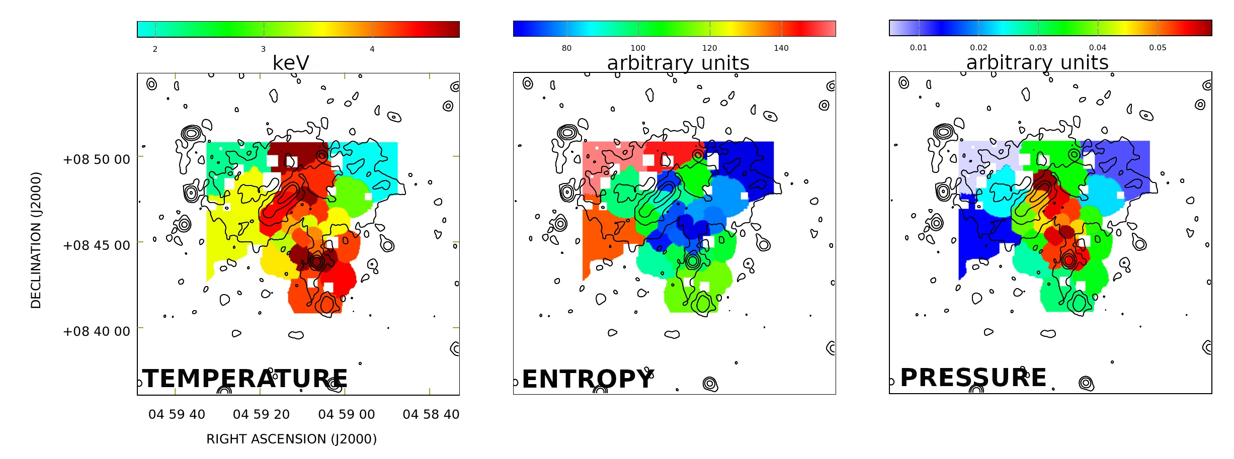
Figure 10: Temperature (left panel), entropy (middle panel), and pressure (right panel) images in colors, taken from Cova et al. (2019). While temperature is shown in keV, entropy and pressure are shown in arbitrary units. Contours represent the radio brightness at 144 MHz at 20^′′, start at 3$\sigma$ ($\sigma=0.4\,$mJy/beam) and increase by a factor 4. They have been derived from the LOFAR images presented in this work. The field of view is the same in all the images.

The behaviour observed in A523 differs from what observed for other clusters, i.e., A520 (Govoni et al., 2001b; Hoang et al., 2019) and 1E 0657-55.8 (Shimwell et al., 2014), which appear to be characterized by respectively an almost flat correlation or by not significant correlation at all. Indeed, a steeper sub-linear correlation emerges when brighter X-ray regions are excluded from statistics, although this correlation is weak. The behaviour observed in this system could reflect the complexity of the dynamical state of the system. The cluster is undergoing a primary merger along the SSW-NNE direction (Girardi et al., 2016; Golovich et al., 2019) and likely a secondary merger along the ESE-WNW direction (Cova et al., 2019). The flat component, weaker in radio, could be related to the primary merger brighter in X-rays. Our LOFAR data show a faint emission emerging in the north-east and in the south of the system, completely buried by the noise at higher frequencies. The steep component corresponds to regions stronger in radio and less bright in X-rays, being likely dominated by the emission in the north of the system. This structure is co-spatial with the possible secondary merger and the higher radio brightness associated with it could be the result of the superposition of the two mergers at this location. While the radio plasma along the SSW-NNE direction is accelerated only by the primary merger and only visible at LOFAR frequencies likely due to ageing, the radio plasma in the perpendicular direction gains energy also through the secondary merger, likely explaining the observed higher radio brightness.

6.2 Radio emission and cluster mass

The mass of clusters hosting radio halos correlates with the radio-halo power at 1.4 GHz (e.g., Yuan et al., 2015), and at 150 MHz (e.g., van Weeren et al., 2021). Numerical simulations show that the SZ effect is an excellent proxy of the cluster mass, with an intrinsic scatter of $\lesssim 10\%$ (e.g., Nagai, 2006), even if recent observations found a scatter up to $\sim$13% that can be significantly reduced when non-thermal pressure associated with ICM turbulent motions are taken into account (e.g., Yu et al., 2015). Galaxy cluster masses derived from X-ray observations can be affected by the dynamical state of the system. The cluster might be in the adiabatic expansion phase and, in this case, X-ray proxies such as luminosity and temperature could be lower than during the initial state, causing an underestimate of the mass of the system (see e.g., Ricker & Sarazin, 2001) with a bias up to $\sim$30% (e.g., Nagai et al. 2007). No SZ mass estimate is available for A523 and the X-ray derived mass is $M_{\rm X,500}=2.2-3.6\times 10^{14}\,M_{\odot}$. Considering our flux measurements at 1.410 GHz and 144 MHz, taking into account the different cosmology, the frequency scaling when appropriate, and k-correction, the value predicted according to the $P_{\rm 1.4\,GHz}-M_{\rm X,500}$ scaling relation in Yuan et al. (2015) is $M_{\rm 500}\,\approx\,6-10\,\times\,10^{14}\,M_{\odot}$, while $M_{\rm 500}\,\approx\,6-9\,\times\,10^{14}\,M_{\odot}$ from the best fit relations $P_{\rm 150\,GHz}-M_{\rm SZ,500}$ by van Weeren et al. (2021).

The values derived are larger than the mass obtained from X-ray observations. Concerning the estimate from 144 MHz data and the van Weeren et al. (2021) scaling relation, we stress that the scaling relation is based on SZ data, while the mass estimate we are using here is derived from X-rays. If we assume that the observed X-ray mass is underestimated by about 30%, we expect a mass of the system of $M_{\rm 500}\,\sim\,5\,\times\,10^{14}\,M_{\odot}$, still lower than the value obtained from the scaling relation. In all these derivations the uncertainties both in the scaling relations and in our radio powers have been taken into account.

Based on $\sigma_{\rm v}$-mass scaling relations from optical data, Girardi et al. (2016) derive a cluster mass $M_{\rm 500}=5-6\times 10^{14}\,M_{\odot}$ that is in better agreement with the values predicted by the radio power of the diffuse emission if this is a radio halo. We note that the uncertainty of the optical mass estimate varies between 7% and 30%.

Overall, we find that the source remains outside the observed correlation both at 1.4 GHz and 144 MHz. However, we note that the scaling relation is not well constrained in the mass range of A523, because most of present studies rely on high mass clusters. We need therefore to extrapolate the correlation in a poorly sampled region of the radio brightness-mass diagram. Moreover, the emission we observe in A523 could be the result of a superposition of different sources (diffuse emission associated with the two merger processes, but also the patch P and the filaments F1, F2 and F3, which may not belong to the radio halo). An estimation of the flux density associated with the filaments is very difficult because these structures are embedded in the diffuse large scale emission.

6.3 Radio brightness versus temperature, entropy and pressure

We compared the radio brightness distribution at 144 MHz with the temperature $T$, pressure $P$ and pseudo-entropy $s$ images of the thermal gas by Cova et al. (2019). As stated in that paper, temperatures $T$ are directly derived through the spectral fitting, while the pressure $P$ and the entropy $s$ are calculated following Rossetti et al. (2007)

$$P=T\times{\rm EM}^{1/2}\,{\rm keV\,cm^{-5/2}\,arcmin^{-1}}$$ (2)

and

$$s=T\times{\rm EM}^{-1/3}\,{\rm keV\,cm^{5/3}\,arcmin^{-2/3}},$$ (3)

where EM is the projected emission measure. Both pressure and entropy values are pseudo quantities, meaning that they are projected along the line of sight.

In Fig. 10 we show the overlay between the radio brightness at 144 MHz at 20^′′ and the temperature (first column), the entropy (second column), and the pressure (third column). Temperature and entropy decrease going from the south of the cluster towards the center, and increase again moving further to the north. The radio emission mainly sits in the north of the cluster starting from the location where temperature and entropy increase again. A low entropy strip with values $<80$ (arbitrary units) cuts the cluster in two parts, one hosting bright radio emission and one with very little radio emission. This strip has the same spatial location as the filament F2 and as part of F1. The pressure image is characterized by an elongation in the SSW-NNE, following the merger axis, with larger pressure values along the filament F3. Moreover, an enhancement in the temperature, entropy and pressure images can be identified corresponding to patch P, indicating that this region is dynamically active and therefore favours a possible interpretation as a phoenix source or a revived fossil plasma.

Overall, the bulk of the radio emission is perpendicular to the main elongation in temperature, entropy and pressure, even if a minor elongation of these three thermodynamic quantities can be identified in the same direction of the brightest regions in radio. Moreover, a hint of a pressure gradient seems to be present at the location of the tail of source S1. Available data and the current analysis are not suitable to discriminate whether this could, or could not, be linked to the diffuse emission on large scales observed in this system. Further analysis is left to follow-up works.

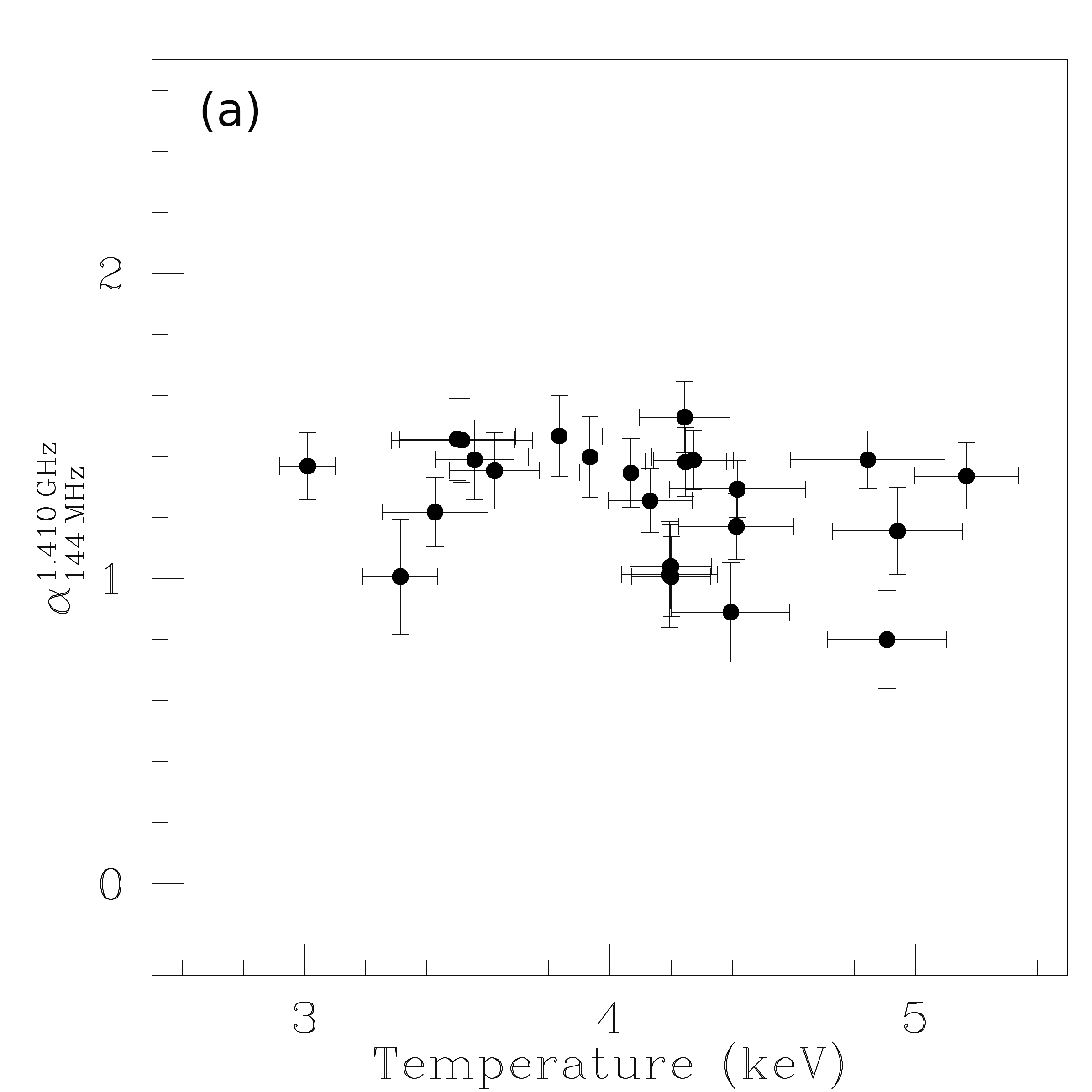
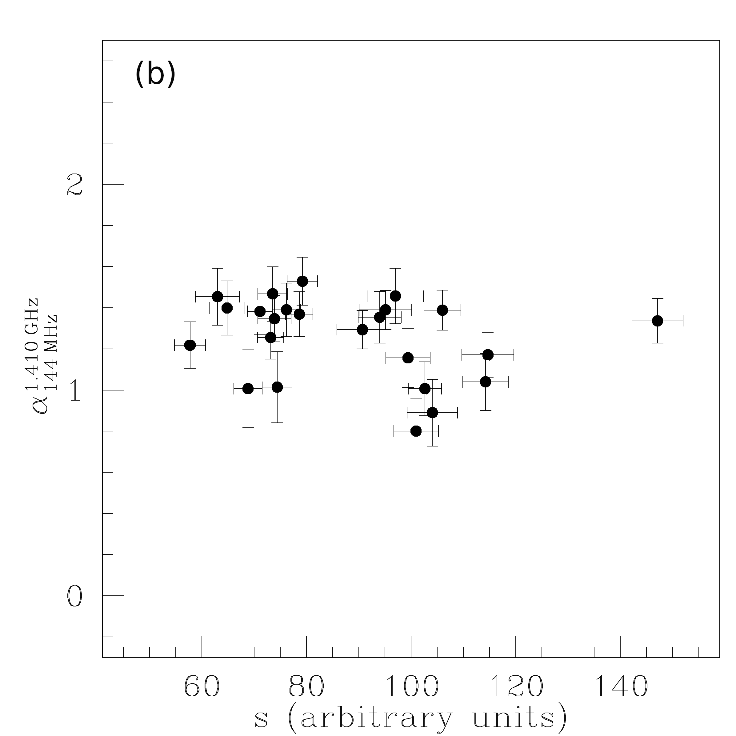
Figure 11: Panel (a): Spectral index between 1.410 GHz and 144 MHz versus thermal gas temperature of the cluster. Panel (b): Spectral index between 1.410 GHz and 144 MHz versus thermal gas pseudo-entropy of the cluster. These plots have been obtained with the low-resolution spectral index images averaged in the same regions of the thermodynamic maps. The temperature and pseudo-entropy values are from Cova et al. (2019).

6.4 Spectral index versus temperature and entropy

Mergers can boost the X-ray luminosity and temperature of a cluster (Ricker & Sarazin, 2001; ZuHone, 2011). If a fraction of the gravitational energy dissipated during the merger is available to re-accelerate radio emitting particles, high temperature and entropy regions may be expected to have a flatter spectrum. The study of any correlation between thermodynamic X-ray quantities and spectral index of diffuse radio emission in galaxy clusters has been conducted only for a limited number of clusters and present results are controversial. An anti-correlation between spectral index and temperature is indicated by the results reported by Feretti et al. (2012), who analyzed clusters with $T<8$ keV, $8<T<10$ keV and $T>10$ keV and derived a trend of decreasing average spectral index for the three samples. A detailed investigation reveals this effect in the cluster A2744 in regions of very different temperatures, spanning from about 5 keV up to more than 10 keV (Orrú et al., 2007). However, Pearce et al. (2017) in A2744 and Shimwell et al. (2014) in the 1E 0657-55.8 cluster do not find significant evidence of this link. Finally, a possible evidence of anti-correlation between spectral index and pseudo-entropy in A2255 has been found by Botteon et al. (2020). In order to better understand the presence of a possible anti-correlation between spectral index and thermodynamic quantities in galaxy clusters, we need to investigate a larger statistical sample.

In Fig. 11, we plot temperature (panel (a)) and pseudo-entropy (panel (b)) against the spectral index. In these plots, the spectral index and the thermodynamic quantities have been averaged in the same regions shown in Fig. 6 in Cova et al. (2019). These plots do not show any clear anti-correlation. The Pearson and Spearman correlation coefficients are $r_{\rm P}=-0.28$ and $r_{\rm S}=-0.30$, and $r_{\rm P}=-0.26$ and $r_{\rm S}=-0.33$, respectively for the two plots. Therefore, if any relation is present, it is likely very weak.

The lack of any link may be due to the fact that entropy is a tracer not only of merger shocks, but also of physical processes occurring in the ICM, as heating/cooling processes. Moreover, in this cluster, the temperature and the entropy show relatively small variations, with values between 3 and 5 keV and 50 and 150 (arbitrary units), compared e.g. to A2744 and A2255, therefore the lack of relations between spectral index and temperature and entropy is not inconsistent with previous findings.

7 Discussion

Historically the most prominent diffuse source in A523 has been classified as a radio halo (Giovannini et al., 2011). Subsequent observations revealed some peculiarities (Girardi et al., 2016; Cova et al., 2019):

1. the radio peak of the source is displaced with respect to the X-ray peak of the system;

2. the source shows filaments of polarized emission up to 15-20%;

3. the radio emission at 1.4 GHz and 144 MHz shows a weak local correlation with the X-rays in the energy range 0.5-2.5 keV;

4. the radio emission at 1.4 GHz does not follow the correlation with the global luminosity $L_{\rm X,0.1-2.4\,keV}$ observed for other radio halos;

5. the radio emission at 1.4 GHz and 144 MHz does not follow the correlation with the mass $M_{\rm 500}$ observed for other radio halos.

In the following we discuss three possible scenarios for the origin of this radio source in light of our results.

Scenario 1. The diffuse emission in A523 could be due to turbulence associated with the complex dynamical state of the system caused by the main and a possible secondary merger. The local radio-X-ray comparison at 144 MHz suggests that the primary merger powers diffuse radio emission along the SSW-NNE direction, as shown by the LOFAR observations, while the secondary merger further energizes particles along ESE-WNW, characterized by higher radio brightness than emission in the north-east and in the south-east and clearly detected both at 144 MHz and at 1.4 GHz.

Scenario 2. The observed radio emission could be the revival of fossil plasma seeded by the central AGN S1 and later re-accelerated by the merger. In this case the correlations observed for radio halos are not expected. LOFAR images reveal several examples of systems where the AGN plasma has spread cosmic ray electrons over large areas (several hundreds of kpc), as recently observed by Brienza et al. (2021), especially in presence of merger turbulence and shocks (e.g., Mandal et al., 2020). However, revived fossil plasma sources and phoenixes typically have a size of 300–400 kpc and steep spectral indices ($\alpha\gtrsim 1.5$, see Mandal et al. 2020 as well as van Weeren et al. 2019 for a review), different from what is observed in A523.

Scenario 3. The lack of an overall radio-X correlation could suggest that radio and the thermal plasma do not occupy the same volume, with the radio emission being a relic seen in projection, as proposed first by van Weeren et al. (2011). A small inclination of the merging axis with respect to the line of sight ($\lesssim$10-20^∘) could explain why a shock wave and a spectral gradient have been not observed. In cosmological simulations, face-on relics show complex morphologies that consist of filaments, possibly polarized, similar to the diffuse source in A523 (e.g., Skillman et al., 2013; Wittor et al., 2019; Wittor, 2021). In these simulations, the spectral indices vary across the relics’ surfaces, but they lack the typical spectral steepening towards the cluster center. However, this scenario is not supported by redshift data since there is no evidence for a merger along the line of sight (Girardi et al., 2016; Golovich et al., 2019). Alternatively, an undetected component along the line of sight could be present if the merger is at the turnaround point or if the possible secondary merger is not entirely in the plane of the sky.

8 Conclusions

In this paper we studied the properties of the diffuse emission in A523 by using new LOFAR observations at 144 MHz and new VLA data at 1.410 and 1.782 GHz. Our finding can be summarized as follows.

The new radio data reveal an unprecedented amount of detail about the properties of the source at radio wavelengths. The emission at 144 MHz appears more extended than at 1.4 GHz, with a total flux density $S_{\rm 144\,MHz}=(1.52\pm 0.31)$ Jy and a size of about 15^′ (i.e., 1.8 Mpc). The source is characterized by a complex morphology consisting of three bright filaments, two in the north of the system already known from previous observations at 1.4 GHz, and a third one developing from the bright northern structure to the south of the cluster. The brightest region of the emission is elongated in the ESE-WNW direction also at 144 MHz. Thanks to the new LOFAR data, we detect for the first time additional regions of faint emission along SSW-NNE and a bright diffuse synchrotron patch in the south, characterized by a steep spectral index and of unclear origin. A local comparison of the radio and X-ray signal suggests the presence of two components, one brighter in X-ray and less bright in radio and the second the other way around. The new LOFAR and VLA data permit, for the first time, an investigation of the spectral properties of the source. Globally, we derive an average spectral index $\alpha_{\rm 144\,MHz}^{\rm 1.410\,GHz}\,=\,1.2\,\pm\,0.1$ with a spectral steepening moving towards higher frequency. The spectral index does not show radial steepening but rather a complex spatial distribution.

Overall, our findings suggest that we are observing the overlapping of different structures, powered by the turbulence associated with the primary and a possible secondary merger. Our results and the current optical data do not support a relic interpretation of the source as a whole, while the relic nature of the northern filaments as well as the revived fossil plasma scenario can not be excluded. Although we have derived valuable information about this complex source from the new radio data, additional optical and X-rays observations are necessary to better understand the geometry of the merger and to verify or exclude the presence of possible components along the line of sight.

Data availability

The data underlying this article will be shared on reasonable request to the corresponding author.

References

- Akamatsu et al. (2013) Akamatsu H., Inoue S., Sato T., Matsusita K., Ishisaki Y., Sarazin C. L., 2013, PASJ, 65, 89
- Bagchi et al. (2006) Bagchi J., Durret F., Neto G. B. L., Paul S., 2006, Science, 314, 791
- Blandford & Ostriker (1978) Blandford R. D., Ostriker J. P., 1978, ApJ, 221, L29
- Bonafede et al. (2009) Bonafede A., et al., 2009, A&A, 503, 707
- Botteon et al. (2020) Botteon A., et al., 2020, ApJ, 897, 93
- Brienza et al. (2017) Brienza M., et al., 2017, A&A, 606, A98
- Brienza et al. (2021) Brienza M., et al., 2021, Nature Astronomy,
- Brown & Rudnick (2011) Brown S., Rudnick L., 2011, MNRAS, 412, 2
- Brown et al. (2011) Brown S., Duesterhoeft J., Rudnick L., 2011, ApJ, 727, L25
- Brunetti & Jones (2014) Brunetti G., Jones T. W., 2014, International Journal of Modern Physics D, 23, 1430007
- Cassano et al. (2010) Cassano R., Ettori S., Giacintucci S., Brunetti G., Markevitch M., Venturi T., Gitti M., 2010, ApJ, 721, L82
- Cassano et al. (2013) Cassano R., et al., 2013, ApJ, 777, 141
- Clarke & Ensslin (2006) Clarke T. E., Ensslin T. A., 2006, AJ, 131, 2900
- Condon et al. (1998) Condon J. J., Cotton W. D., Greisen E. W., Yin Q. F., Perley R. A., Taylor G. B., Broderick J. J., 1998, AJ, 115, 1693
- Cova et al. (2019) Cova F., et al., 2019, A&A, 628, A83
- Cuciti et al. (2021) Cuciti V., et al., 2021, A&A, 647, A51
- Deiss et al. (1997) Deiss B. M., Reich W., Lesch H., Wielebinski R., 1997, A&A, 321, 55
- Di Gennaro et al. (2018) Di Gennaro G., et al., 2018, ApJ, 865, 24
- Drury (1983) Drury L. O., 1983, Reports on Progress in Physics, 46, 973
- Eckert et al. (2016) Eckert D., Jauzac M., Vazza F., Owers M. S., Kneib J. P., Tchernin C., Intema H., Knowles K., 2016, MNRAS, 461, 1302
- Einasto et al. (2001) Einasto M., Einasto J., Tago E., Müller V., Andernach H., 2001, AJ, 122, 2222
- Ensslin et al. (1998) Ensslin T. A., Biermann P. L., Klein U., Kohle S., 1998, A&A, 332, 395
- Erler et al. (2015) Erler J., Basu K., Trasatti M., Klein U., Bertoldi F., 2015, MNRAS, 447, 2497
- Feretti et al. (2004) Feretti L., Orrù E., Brunetti G., Giovannini G., Kassim N., Setti G., 2004, A&A, 423, 111
- Feretti et al. (2012) Feretti L., Giovannini G., Govoni F., Murgia M., 2012, A&ARv, 20, 54
- Giacintucci et al. (2005) Giacintucci S., et al., 2005, A&A, 440, 867
- Giovannini et al. (1993) Giovannini G., Feretti L., Venturi T., Kim K. T., Kronberg P. P., 1993, ApJ, 406, 399
- Giovannini et al. (2009) Giovannini G., Bonafede A., Feretti L., Govoni F., Murgia M., Ferrari F., Monti G., 2009, A&A, 507, 1257
- Giovannini et al. (2011) Giovannini G., Feretti L., Girardi M., Govoni F., Murgia M., Vacca V., Bagchi J., 2011, A&A, 530, L5
- Girardi et al. (2016) Girardi M., et al., 2016, MNRAS, 456, 2829
- Golovich et al. (2019) Golovich N., et al., 2019, ApJ, 882, 69
- Govoni et al. (2001a) Govoni F., Enßlin T. A., Feretti L., Giovannini G., 2001a, A&A, 369, 441
- Govoni et al. (2001b) Govoni F., Feretti L., Giovannini G., Böhringer H., Reiprich T. H., Murgia M., 2001b, A&A, 376, 803
- Govoni et al. (2005) Govoni F., Murgia M., Feretti L., Giovannini G., Dallacasa D., Taylor G. B., 2005, A&A, 430, L5
- Govoni et al. (2013) Govoni F., Murgia M., Xu H., Li H., Norman M. L., Feretti L., Giovannini G., Vacca V., 2013, A&A, 554, A102
- HI4PI Collaboration et al. (2016) HI4PI Collaboration et al., 2016, A&A, 594, A116
- Hales et al. (1988) Hales S. E. G., Baldwin J. E., Warner P. J., 1988, MNRAS, 234, 919
- Hales et al. (1990) Hales S. E. G., Masson C. R., Warner P. J., Baldwin J. E., 1990, MNRAS, 246, 256
- Hardcastle et al. (2021) Hardcastle M. J., et al., 2021, A&A, 648, A10
- Hoang et al. (2019) Hoang D. N., et al., 2019, A&A, 622, A20
- Hodgson et al. (2020) Hodgson T., Johnston-Hollitt M., McKinley B., Vernstrom T., Vacca V., 2020, arXiv e-prints, p. arXiv:2007.10578
- Hurley-Walker (2017) Hurley-Walker N., 2017, arXiv e-prints, p. arXiv:1703.06635
- Intema et al. (2017) Intema H. T., Jagannathan P., Mooley K. P., Frail D. A., 2017, A&A, 598, A78
- Kale & Dwarakanath (2010) Kale R., Dwarakanath K. S., 2010, ApJ, 718, 939
- Kang et al. (2012) Kang H., Ryu D., Jones T. W., 2012, ApJ, 756, 97
- Large et al. (1959) Large M. I., Mathewson D. S., Haslam C. G. T., 1959, Nature, 183, 1663
- Liang et al. (2000) Liang H., Hunstead R. W., Birkinshaw M., Andreani P., 2000, ApJ, 544, 686
- Lindner et al. (2014) Lindner R. R., et al., 2014, ApJ, 786, 49
- Loi et al. (2019) Loi F., et al., 2019, MNRAS, 490, 4841
- Mandal et al. (2020) Mandal S., et al., 2020, A&A, 634, A4
- Markevitch et al. (2005) Markevitch M., Govoni F., Brunetti G., Jerius D., 2005, ApJ, 627, 733
- Murgia (1996) Murgia M., 1996, PhD thesis, University of Bologna
- Myers (2003) Myers Jerome L.; Well A. D., 2003, printdisabled; librarygenesis,Library Genesis, p. 508
- Nagai (2006) Nagai D., 2006, ApJ, 650, 538
- Nagai et al. (2007) Nagai D., Vikhlinin A., Kravtsov A. V., 2007, ApJ, 655, 98
- Norris et al. (2021) Norris R. P., et al., 2021, Publ. Astron. Soc. Australia, 38, e003
- Offringa et al. (2014) Offringa A. R., McKinley B., Hurley-Walker et al., 2014, MNRAS, 444, 606
- Orrú et al. (2007) Orrú E., Murgia M., Feretti L., Govoni F., Brunetti G., Giovannini G., Girardi M., Setti G., 2007, A&A, 467, 943
- Pacholczyk (1970) Pacholczyk A. G., 1970, Radio astrophysics. Nonthermal processes in galactic and extragalactic sources, Series of Books in Astronomy and Astrophysics.. Freeman, San Francisco
- Parekh et al. (2017) Parekh V., Dwarakanath K. S., Kale R., Intema H., 2017, MNRAS, 464, 2752
- Pearce et al. (2017) Pearce C. J. J., et al., 2017, ApJ, 845, 81
- Pearson (1895) Pearson K., 1895, Proceedings of the Royal Society of London Series I, 58, 240
- Perley & Butler (2013) Perley R. A., Butler B. J., 2013, ApJS, 204, 19
- Perley & Butler (2017) Perley R. A., Butler B. J., 2017, ApJS, 230, 7
- Pizzo et al. (2011) Pizzo R. F., de Bruyn A. G., Bernardi G., Brentjens M. A., 2011, A&A, 525, A104
- Planck Collaboration et al. (2013) Planck Collaboration et al., 2013, A&A, 554, A140
- Planck Collaboration et al. (2020) Planck Collaboration et al., 2020, A&A, 641, A6
- Rajpurohit et al. (2018) Rajpurohit K., et al., 2018, ApJ, 852, 65
- Rajpurohit et al. (2020) Rajpurohit K., et al., 2020, A&A, 642, L13
- Rajpurohit et al. (2021a) Rajpurohit K., et al., 2021a, A&A, 646, A56
- Rajpurohit et al. (2021b) Rajpurohit K., et al., 2021b, A&A, 646, A135
- Ricker & Sarazin (2001) Ricker P. M., Sarazin C. L., 2001, ApJ, 561, 621
- Rossetti et al. (2007) Rossetti M., Ghizzardi S., Molendi S., Finoguenov A., 2007, A&A, 463, 839
- Rottgering et al. (1997) Rottgering H. J. A., Wieringa M. H., Hunstead R. W., Ekers R. D., 1997, MNRAS, 290, 577
- Schneider (2015) Schneider P., 2015, Extragalactic Astronomy and Cosmology: An Introduction. Springer-Verlag, Berlin
- Shi et al. (2020) Shi X., Nagai D., Aung H., Wetzel A., 2020, MNRAS, 495, 784
- Shimwell et al. (2014) Shimwell T. W., Brown S., Feain I. J., Feretti L., Gaensler B. M., Lage C., 2014, MNRAS, 440, 2901
- Shimwell et al. (2019) Shimwell T. W., et al., 2019, A&A, 622, A1
- Skillman et al. (2013) Skillman S. W., Xu H., Hallman E. J., O’Shea B. W., Burns J. O., Li H., Collins D. C., Norman M. L., 2013, ApJ, 765, 21
- Smirnov & Tasse (2015) Smirnov O. M., Tasse C., 2015, MNRAS, 449, 2668
- Spearman (1904) Spearman C., 1904, American Journal of Psychology 15, p. 72–101
- Tasse (2014a) Tasse C., 2014a, arXiv e-prints, p. arXiv:1410.8706
- Tasse (2014b) Tasse C., 2014b, A&A, 566, A127
- Tasse et al. (2018) Tasse C., et al., 2018, A&A, 611, A87
- Tasse et al. (2021) Tasse C., et al., 2021, A&A, 648, A1
- Thierbach et al. (2003) Thierbach M., Klein U., Wielebinski R., 2003, A&A, 397, 53
- Urdampilleta et al. (2018) Urdampilleta I., Akamatsu H., Mernier F., Kaastra J. S., de Plaa J., Ohashi T., Ishisaki Y., Kawahara H., 2018, A&A, 618, A74
- Vacca et al. (2010) Vacca V., Murgia M., Govoni F., Feretti L., Giovannini G., Orrù E., Bonafede A., 2010, A&A, 514, A71
- Vacca et al. (2014) Vacca V., Feretti L., Giovannini G., Govoni F., Murgia M., Perley R. A., Clarke T. E., 2014, A&A, 561, A52
- Vacca et al. (2018a) Vacca V., Murgia M., Govoni F., Enßlin T., Oppermann N., Feretti L., Giovannini G., Loi F., 2018a, Galaxies, 6, 142
- Vacca et al. (2018b) Vacca V., et al., 2018b, MNRAS, 479, 776
- Voit et al. (2005) Voit G. M., Kay S. T., Bryan G. L., 2005, MNRAS, 364, 909
- Wittor (2021) Wittor D., 2021, New Astron., 85, 101550
- Wittor et al. (2019) Wittor D., Hoeft M., Vazza F., Brüggen M., Domínguez-Fernández P., 2019, MNRAS, 490, 3987
- Xie et al. (2020) Xie C., et al., 2020, A&A, 636, A3
- Yu et al. (2015) Yu L., Nelson K., Nagai D., 2015, ApJ, 807, 12
- Yuan et al. (2015) Yuan Z. S., Han J. L., Wen Z. L., 2015, ApJ, 813, 77
- Zhang et al. (2020) Zhang X., et al., 2020, A&A, 642, L3
- ZuHone (2011) ZuHone J. A., 2011, ApJ, 728, 54
- de Gasperin et al. (2015) de Gasperin F., Intema H. T., van Weeren R. J., Dawson W. A., Golovich N., Wittman D., Bonafede A., Brüggen M., 2015, MNRAS, 453, 3483
- de Gasperin et al. (2018) de Gasperin F., Intema H. T., Frail D. A., 2018, MNRAS, 474, 5008
- de Gasperin et al. (2019) de Gasperin F., et al., 2019, A&A, 622, A5
- van Weeren et al. (2011) van Weeren R. J., Brüggen M., Röttgering H. J. A., Hoeft M., Nuza S. E., Intema H. T., 2011, A&A, 533, A35
- van Weeren et al. (2016a) van Weeren R. J., et al., 2016a, ApJS, 223, 2
- van Weeren et al. (2016b) van Weeren R. J., et al., 2016b, ApJ, 818, 204
- van Weeren et al. (2019) van Weeren R. J., de Gasperin F., Akamatsu H., Brüggen M., Feretti L., Kang H., Stroe A., Zandanel F., 2019, Space Sci. Rev., 215, 16
- van Weeren et al. (2021) van Weeren R. J., et al., 2021, A&A, 651, A115