Lipschitz continuity of the Hausdorff dimension of self-affine sponges at Sierpinski sponges

Abstract.

The Hausdorff dimension of general Sierpinski carpets, [4] and [20], and the generalization on Lalley-Gatzouras carpets, [10], are today well known results, the formulas being obtain via the variational principle for the dimension. We call the multidimensional versions of these carpets Sierpinski sponges and self-affine sponges, respectively,. In this paper we show that the Hausdorff dimension of self-affine sponges, defined in $\mathrm{R}^{3}$, is a Lipschitz continuous function at Sierpinski sponges.

1. Introduction and statements

The dimension theory of $C^{1+\alpha}$ conformal repellers is well understood by means of the thermodynamic formalism introduced by Sinai-Ruelle-Bowen [24], [23], [5] and the famous Bowen’s equation [6], [22]. In particular there is a unique ergodic measure of full dimension which is a Gibbs state.

The dimension theory of non-conformal repellers is still being developed and no such general formalism exists. The computation of Hausdorff dimension of non-conformal fractals began with the fundamental works by Bedford [4] and McMullen [20] on the general Sierpinski carpets, and their generalization [10] on the Lalley-Gatzouras carpets, as they are known today. See also [1] for an extension of the Lalley-Gatzouras carpets. These are self-affine fractals in the plane and there is an ergodic measure of full dimension, in fact Bernoulli (such a measure is, in general, not unique for Lalley-Gatzouras carpets [2]). There are also some non-linear versions of these results, [11], [15], [17] and [19], towards a Dimension Formalism for these kind of non-conformal repellers. In particular, in [15] and [19] we compute the Hausdorff dimension of Non-linear Lalley-Gatzouras carpets which, as the name suggests, are the $C^{1+\alpha}$ non-linear versions of the Lalley-Gatzouras carpets.

Other approaches try to give a formula for the Hausdorff dimension in a generic setting, instead of considering particular families as before. One such example is the famous Falconer’s formula [8] which gives, under some hypotheses, the Hausdorff dimension of the self-affine fractal for ‘almost every’ translation vector-parameters, but does not tell for which parameters it holds (exceptions being the self-affine fractals in the plane considered in [12] and its non-linear versions [16]). In fact these two approaches are quite different, for the self-affine fractals for which Falconer’s formula holds there is coincidence with Hausdorff and box-counting dimensions, as for the Lalley-Gatzouras carpets these two dimensions do not coincide in general [10]. More recently, Hochmann and Rapaport [13] gave a formula for the Hausdorff dimension of self-affine sets in the plane satisfying an irreducibility condition and an exponential separation condition.

The computation of the Hausdorff dimension of non-conformal fractals in $\mathbb{R}^{d}$, $d>2$ reveals to be a much more difficult task. There is a natural way of defining the $d$-dimensional versions of general Sierpinski carpets and Lalley-Gatzouras carpets which we shall call, respectively, Sierpinski sponges and self-affine sponges. Recently, in a major breakthrough, [7] showed that the variational principle for the dimension does not hold, in general, within the class of Baranski sponges (even for $d=3$), i.e. there is not an ergodic measure of full dimension. They showed that the Hausdorff dimension in that class can be calculated via pseudo-Bernoulli measures. On the other hand, Kenyon and Peres [14] computed the Hausdorff dimension of Sierpinski sponges by proving the variational principle for the dimension and, moreover, there is a unique ergodic measure of full Hausdorff dimension, in fact Bernoulli (see also [9], and see [3] for a random version). We do not know if the variational principle for the dimension holds for self-affine sponges that are close to Sierpinski sponges but we will show that the Hausdorff dimension of self-affine sponges, $d=3$, is Lipschitz continuous at Sierpinski sponges. Since the variational principle for the dimension holds for Sierpinski sponges, this implies that the variational principle for the dimension almost holds for self-affine sponges close to Sierpinski sponges. We notice that the continuity of the Hausdorff dimension in the class of Baranski sponges was proved in [7], but the class of self-affine sponges considered in this paper need not be Baranski sponges. Also by restricting to the continuity of Hausdorff dimension at Sierpinski sponges we are able to obtain more explicit and quantitative results.

1.1. Sierpinski sponges

We begin by describing the Sierpinski sponges studied in [14] (the multidimensional versions of the general Sierpinski carpets). Let $\mathbb{T}^{d}=\mathbb{R}^{d}/\mathbb{Z}^{d}$ be the $d$-dimensional torus and $f\colon\mathbb{T}^{d}\to\mathbb{T}^{d}$ be given by

$$f(x_{1},.x_{2},...,x_{d})=(l_{1}x_{1},l_{2}x_{2},...,l_{d}x_{d})$$

where $l_{1}\geq l_{2}\geq...\geq l_{d}>1$ are integers. The grids of hyperplanes

$$\{i/l_{1}\}\times[0,1]^{d-1}, \,i=0,...,l_{1}-1$$

$$[0,1]\times\{i/l_{2}\}\times[0,1]^{d-2}, \,i=0,...,l_{2}-1$$

$$\vdots$$

$$[0,1]^{d-1}\times\{i/l_{d}\}, \,i=0,...,l_{d}-1$$

form a set of boxes each of which is mapped by $f$ onto the entire torus (these boxes are the domains of invertibility of $f$). Now choose some of these boxes and consider the fractal set $\Lambda$ consisting of those points that always remain in these chosen boxes when iterating $f$. Geometrically, $\Lambda$ is the limit (in the Hausdorff metric), or the intersection, of $n$-approximations: the 1-approximation consists of the chosen boxes; the 2-approximation consists in replacing each box of the 1-approximation by a rescaled affine copy of the 1-approximation, resulting in more and smaller boxes; the 3-approximation consists in replacing each box of the 2-approximation by a rescaled affine copy of the 1-approximation, and so on. We say that $\Lambda$ is a Sierpinski sponge, and their Hausdorff dimension was computed in [14] (a formula is given in next section).

1.2. Self-affine sponges

Now we describe the self-affine sponges (the multidimensional versions of Lalley-Gatzouras carpets), which include as a very particular case the Sierpinski sponges. Let $S_{1},S_{2},...,S_{r}$ be contractions of $\mathbb{R}^{d}$. Then there is a unique nonempty compact set $\Lambda$ of $\mathbb{R}^{d}$ such that

$$\Lambda=\bigcup_{i=1}^{r}S_{i}(\Lambda).$$

We will refer to $\Lambda$ as the limit set of the semigroup generated by $S_{1},S_{2},...,S_{r}$. We are going to consider sets $\Lambda$ which are limit sets of the semigroup generated by the $d$-dimensional mappings $A_{i^{1}i^{2}...i^{d}}$ given by

$$A_{i^{1}i^{2}...i^{d}}=\begin{pmatrix}a_{i^{1}i^{2}...i^{d}}&0&0&\cdots&0\\ 0&a_{i^{1}i^{2}...i^{d-1}}&0&\cdots&0\\ &\vdots&\\ 0&\cdots&0&0&a_{i^{1}}\end{pmatrix}x+\begin{pmatrix}u_{i^{1}i^{2}...i^{d}}\\ u_{i^{1}i^{2}...i^{d-1}}\\ \vdots\\ u_{i^{1}}\end{pmatrix}$$

for $(i^{1},i^{2},...,i^{d})\in\mathcal{I}$. Here

$$\mathcal{I}=\{(i^{1},i^{2},...,i^{d}):\; 1\leq i^{1}\leq m\,,\,1\leq i^{2}\leq m_{i^{1}},$$

$$1\leq i^{3}\leq m_{i^{1}i^{2}}\,,...,\,1\leq i^{d}\leq m_{i^{1}i^{2}...i^{d-1}}\}$$

is a finite index set, and $0<a_{i^{1}...i^{k}}<1\,,\,k=1,...,d$ satisfy

$$a_{i^{1}...i^{k}i^{k+1}}\leq a_{i^{1}...i^{k}}\,.$$

Also, for each $(i^{1},...,i^{d})\in\mathcal{I}$ and $k\in\{1,...,d\}$,

$$\sum_{i^{k}=1}^{m_{i^{1}...i^{k-1}}}a_{i^{1}...i^{k}}\leq 1$$

(when $k=1$ the end of the sum is $m$) and

$$0\leq u_{i^{1}...i^{k}}<u_{i^{1}...i^{k}+1}<1\,,\quad u_{i^{1}...i^{k}+1}-u_{i^{1}...i^{k}}\geq a_{i^{1}...i^{k}}\,,$$

when $k>1,\,i^{k}=m_{i^{1}...i^{k-1}}$ we substitute $u_{i^{1}...i^{k}+1}$ by 1. These hypotheses guarantee that the boxes

$$R_{i^{1}...i^{d}}=A_{i^{1}...i^{d}}([0,1]^{d})$$

have interiors that are pairwise disjoint, with edges parallel to the coordinate axes, the box $R_{i^{1}...i^{d}}$ having $k^{th}-$edge with length $a_{i^{1}...i^{k}}$. Geometrically, $\Lambda$ is constructed like the Sierpinski sponges, with the 1-approximation consisting of the boxes $R_{i^{1}...i^{d}}$, the 2-approximation consisting in replacing each box of the 1-aproximation by a rescaled affine copy of the 1-approximation, and so on. See Figure 1 for an illustration of the case $d=3$ (where we used $c_{i},\,b_{ij},\,a_{ijk}$ instead of $a_{i^{1}},\,a_{i^{1}i^{2}},\,a_{i^{1}i^{2}i^{3}}$, respectively). When $d=2$ the sets $\Lambda$ are the Lalley-Gatzouras carpets, and their 1-approximation corresponds to the projection onto the $yz$-plane of Figure 1. In general we say that $\Lambda$ is a self-affine sponge.

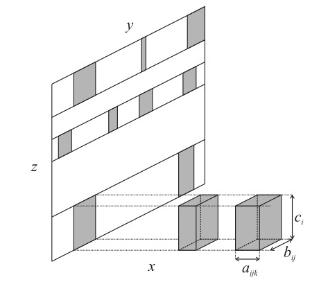
Figure 1. Self-affine sponges

Given ${\bf p}=(p_{i^{1}...i^{d-1}})$ a collection of non-negative numbers satisfying

$$p_{i^{1}...i^{k}}=\sum_{i^{k+1}}p_{i^{1}...i^{k}i^{k+1}}\,,\quad k=d-2,d-3,...,1$$

$$\sum_{i^{1}}p_{i^{1}}=1,$$

we define the numbers $\lambda_{k}({\bf{p}})$, $k=1,...,d-1$ by

$$\lambda_{k}({\bf{p}})=\frac{\underset{i^{1}...i^{k}}{\sum}p_{i^{1}...i^{k}}\log p_{i^{1}...i^{k}}-\underset{i^{1}...i^{k-1}}{\sum}p_{i^{1}...i^{k-1}}\log p_{i^{1}...i^{k-1}}}{\underset{i^{1}...i^{k}}{\sum}p_{i^{1}...i^{k}}\log a_{i^{1}...i^{k}}},$$

(by convention: $0\log 0=0$; for $k=1$ the second sum in the numerator is $0$)
and the number $t(\bf{p})$ as the unique real in $[0,1]$ satisfying

$$\sum_{i^{1}...i^{d-1}}p_{i^{1}...i^{d-1}}\log\left(\sum_{i^{d}}a_{i^{1}...i^{d-1}i^{d}}^{t(\bf{p})}\right)=0.$$

The number $\sum_{k=1}^{d-1}\lambda_{k}({\bf{p}})$ is the Hausdorff dimension in the hyperplane $x_{2}...x_{d}$ of the set of generic points for the distribution ${\bf{p}}$; the number $t(\bf{p})$ is the Hausdorff dimension of a typical $1$-dimensional fibre in the $x_{1}$-direction relative to the distribution ${\bf{p}}$, and is given by a random Moran formula. We will see that the sum of these two numbers is the Hausdorff dimension of a Bernoulli measure supported on $\Lambda$, and so we have the following result.

Theorem 1.

Let $\Lambda$ be a self-affine sponge. Then

$$\operatorname*{\mathrm{dim}_{\mathrm{H}}}\Lambda\geq\sup_{\bf{p}}\left\{\sum_{k=1}^{d-1}\lambda_{k}({\bf{p}})+t({\bf{p}})\right\}.$$ (1)

Here $\operatorname*{\mathrm{dim}_{\mathrm{H}}}\Lambda$ stands for the Hausdorff dimension of a set $\Lambda$.

Problem. When does equality hold in (1)?

In other words, when does the variational principle for the dimension hold, in the class of self-affine sponges? When $d=2$ this corresponds to Lalley-Gatzouras carpets and equality in (1) was proved in [10] (see also [15] for an alternative proof and [18] for a random version). For general $d$ but with $a_{i^{1}...i^{k}}=a^{(k)}$, $k=1,...,d$ this corresponds, essentially, to Sierpinski sponges and equality in (1) was, essentially, proved in [14].

As we know now, by [7], equality in (1) might not hold, in general, even when $d=3$.

For the sake of clarity we will restrict to $d=3$ (even though the results in this paper might extend to general $d$). In this case, we use the simpler notation $c_{i}$ for $a_{i}$, $i=1,...,m$ and $b_{ij}$ for $a_{ij}$, $j=1,...,m_{j}$, keeping the notation for $a_{ijk}$, $k=1,...,m_{ij}$ (see Figure 1).

2. $(a,b,c;\varepsilon)$-sponges

In this section $d=3$.

Definition 1.

We say that a self-affine sponge is an $(a,b,c;\varepsilon)$-sponge, for some numbers $0<a\leq b\leq c<1$, $\varepsilon\geq 0$, if

$$e^{-\varepsilon}\leq\frac{a_{ijk}}{a}\leq e^{\varepsilon},\quad e^{-\varepsilon}\leq\frac{b_{ij}}{b}\leq e^{\varepsilon},\quad e^{-\varepsilon}\leq\frac{c_{i}}{c}\leq e^{\varepsilon},$$

for every $(i,j,k)\in\mathcal{I}$.

The case $\varepsilon=0$ corresponds essentially to what we called Sierpinski sponges (even though the numbers $a,b$ and $c$ need not be integers), and we will still call Sierpinski sponges to this larger class. As said before, their Hausdorff dimension was, essentially, computed in [14] via the variational principle for the dimension. When we are close to a Sierpinski sponge, say an $(a,b,c;\varepsilon)$-sponge with $\varepsilon>0$ small, we do not know if the variational principle for the dimension holds but we know that the Hausdorff dimension is close to the Hausdorff dimension of the Sierpinski sponge $(a,b,c;0)$. When we talk about continuity of the Hausdorff dimension of self-affine sponges it is implicit that their alphabet $\mathcal{I}$ is fixed.

Denote by $\Lambda_{a,b,c}$ a Sierpinski sponge $(a,b,c;0)$, and by $\Lambda_{a,b,c;\varepsilon}$ an $(a,b,c;\varepsilon)-sponge$.

Let $\mathcal{J}=\{(i,j)\colon(i,j,k)\in\mathcal{I}\text{ for some }k\}$. Let

$$\underline{t}=\min_{(i,j)\in\mathcal{J}}\frac{\log m_{ij}}{-\log a}\quad\text{and}\quad\overline{t}=\max_{(i,j)\in\mathcal{J}}\frac{\log m_{ij}}{-\log a}$$

Theorem 2.

Let $\Lambda_{a,b,c}$ be a Sierpinski sponge such that $\underline{t}<\overline{t}$. There exists a constant $C$ (depending only on $a$, $b$, $c$ and $\mathcal{I}$) such that for every $\varepsilon>0$ sufficiently small

$$\operatorname*{\mathrm{dim}_{\mathrm{H}}}\Lambda_{a,b,c}-C\varepsilon\leq\operatorname*{\mathrm{dim}_{\mathrm{H}}}\Lambda_{a,b,c;\varepsilon}\leq\operatorname*{\mathrm{dim}_{\mathrm{H}}}\Lambda_{a,b,c}+C\varepsilon.$$

Remark 1.

Going through the proof of Theorem 2 it is possible to give an explicit expression for $C$, if that is needed for some application, but that is not our purpose in this paper.

The lower estimate in Theorem 2 follows easily from Theorem 1. For the upper estimate in Theorem 2 we will construct a 2-parameter family of Bernoulli measures.

Given $\Lambda$ a self-affine sponge we write

$$\mathrm{VP}(\Lambda)=\sup_{\bf{p}}\left\{\lambda_{1}({\bf{p}})+\lambda_{2}({\bf{p}})+t({\bf{p}})\right\}.$$

Even though we do not know if the variational principle for the dimension holds for $(a,b,c;\varepsilon)$-sponges, $\varepsilon>0$ small, we have the following result.

Corollary 1.

Let $\Lambda_{a,b,c}$ be a Sierpinski sponge such that $\underline{t}<\overline{t}$. There exists a constant $C$ (depending only on $a$, $b$, $c$ and $\mathcal{I}$) such that for every $\varepsilon>0$ sufficiently small

$$\mathrm{VP}(\Lambda_{a,b,c;\varepsilon})\leq\operatorname*{\mathrm{dim}_{\mathrm{H}}}\Lambda_{a,b,c;\varepsilon}\leq\mathrm{VP}(\Lambda_{a,b,c;\varepsilon})+C\varepsilon.$$

The lower estimate in Corollary 1 follows from Theorem 1 and the upper estimate in Corollary 1 follows from the proof of Theorem 2.

3. Proof of Theorem 1

In this part, $d$ is any integer greater than or equal to 2.

There is a natural symbolic representation associated with our system that we shall describe now. Consider the sequence space $\Omega=\mathcal{I}^{\mathbb{N}}$. Elements of $\Omega$ will be represented by $\omega=(\omega_{1},\omega_{2},...)$ where $\omega_{n}=(i^{1}_{n},...,i^{d}_{n})\in\mathcal{I}$. Given $\omega\in\Omega$ and $n\in\mathbb{N}$, let $\omega(n)=(\omega_{1},\omega_{2},...,\omega_{n})$ and define the cylinder of order $n$,

$$C_{\omega(n)}=\{\omega^{\prime}\in\Omega:\omega^{\prime}_{l}=\omega_{l},\,l=1,...,n\},$$

and the basic box of order $n$,

$$R_{\omega(n)}=A_{\omega_{1}}\circ A_{\omega_{2}}\circ\cdots\circ A_{\omega_{n}}([0,1]^{d}).$$

We have that $(R_{\omega(n)})_{n}$ is a decreasing sequence of closed boxes having $k^{th}-$edge with length $\prod_{l=1}^{n}a_{i_{l}^{1}...i_{l}^{k}}$. Thus $\bigcap_{n=1}^{\infty}R_{\omega(n)}$ consists of a single point which belongs to $\Lambda$ that we denote by $\chi(\omega)$. This defines a continuous and surjective map $\chi\colon\Omega\to\Lambda$ which is at most $2^{d}$ to 1, and only fails to be a homeomorphism when some of the boxes $R_{i^{1}...i^{d}}$ have nonempty intersection.

Let $\lambda({\bf{p}})=\sum_{k=1}^{d-1}\lambda_{k}({\bf{p}})$. We shall construct probability measures $\mu_{\bf{p}}$ supported on $\Lambda$ with

$$\operatorname*{\mathrm{dim}_{\mathrm{H}}}\mu_{\bf{p}}=\lambda({\bf{p}})+t(\bf{p}).$$

This gives what we want because $\operatorname*{\mathrm{dim}_{\mathrm{H}}}\Lambda\geq\operatorname*{\mathrm{dim}_{\mathrm{H}}}\mu_{\bf{p}}$.

Let $\tilde{\mu}_{\bf{p}}$ be the Bernoulli measure on $\Omega$ that assigns to each symbol $(i^{1},...,i^{d})\in\mathcal{I}$ the probability

$$p_{i^{1}...i^{d-1}}\,\frac{a_{i^{1}...i^{d}}^{t(\bf{p})}}{\sum_{j^{d}}a_{i^{1}...i^{d-1}j^{d}}^{t(\bf{p})}}.$$

In other words, we have

$$\tilde{\mu}_{\bf{p}}(C_{\omega(n)})=\prod_{l=1}^{n}p_{i_{l}^{1}...i_{l}^{d-1}}\,\frac{a_{i_{l}^{1}...i_{l}^{d}}^{t(\bf{p})}}{\sum_{j^{d}}a_{i_{l}^{1}...i_{l}^{d-1}j^{d}}^{t(\bf{p})}}.$$

Let $\mu_{\bf{p}}$ be the probability measure on $\Lambda$ which is the pushforward of $\tilde{\mu}_{\bf{p}}$ by $\chi$, i.e. $\mu_{\bf{p}}=\tilde{\mu}_{\bf{p}}\circ\chi^{-1}$.

For calculating the Hausdorff dimension of $\mu_{\bf{p}}$, we shall consider some special sets called approximate cubes. Given $\omega\in\Omega$ and $n\in\mathbb{N}$ such that $n\geq(\log\min a_{i^{1}...i^{d}})/(\log\max a_{i^{1}})$, define $L_{n}^{0}(\omega)=n$,

$$L_{n}^{1}(\omega)= \max\left\{k\geq 1:\prod_{l=1}^{n}a_{i_{l}^{1}}\leq\prod_{l=1}^{k}a_{i_{l}^{1}i_{l}^{2}}\right\}$$

$$\vdots$$ (2)

$$L_{n}^{d-1}(\omega)= \max\left\{k\geq 1:\prod_{l=1}^{n}a_{i_{l}^{1}}\leq\prod_{l=1}^{k}a_{i_{l}^{1}...i_{l}^{d}}\right\}$$

and the approximate cube

$$B_{n}(\omega)=\left\{\begin{matrix}\quad\quad\overline{i_{l}^{1}}=i_{l}^{1},\>l=1,...,n\\ \overline{\omega}\in\Omega:\>\,\overline{i_{l}^{2}}=i_{l}^{2},\>l=1,...,L_{n}^{1}(\omega)\\ \quad\quad\quad\quad\vdots\\ \quad\quad\quad\quad\quad\overline{i_{l}^{d}}=i_{l}^{d},\>l=1,...,L_{n}^{d-1}(\omega)\end{matrix}\right\}.$$

We have that each approximate cube $B_{n}(\omega)$ is a finite union of cylinder sets, and that approximate cubes are nested, i.e., given two, say $B_{n}(\omega)$ and $B_{n^{\prime}}(\omega^{\prime})$, either $B_{n}(\omega)\cap B_{n^{\prime}}(\omega^{\prime})=\emptyset$ or $B_{n}(\omega)\subset B_{n^{\prime}}(\omega^{\prime})$ or $B_{n^{\prime}}(\omega^{\prime})\subset B_{n}(\omega)$. Moreover, $\chi(B_{n}(\omega))=\tilde{B}_{n}(\omega)\cap\Lambda$ where $\tilde{B}_{n}(\omega)$ is a closed box in $\mathbb{R}^{d}$ with edges parallel to the coordinate axes, the $k^{th}-$edge with length $\prod_{l=1}^{L_{n}^{k-1}(\omega)}a_{i_{l}^{1}...i_{l}^{k}}$. By (2),

$$1\leq\frac{\underset{l=1}{\overset{L_{n}^{k-1}(\omega)}{\prod}}a_{i_{l}^{1}...i_{l}^{k}}}{\underset{l=1}{\overset{n}{\prod}}a_{i_{l}^{1}}}\leq\max\,a_{i^{1}...i^{d}}^{-1},$$ (3)

for $k=1,...,d$, hence the term “approximate cube”. It follows from (3) that

$$\frac{\sum_{l=1}^{L_{n}^{k-1}(\omega)}\log a_{i^{1}_{l}...i^{k}_{l}}}{\sum_{l=1}^{n}\log a_{i_{l}^{1}}}=1+\frac{1}{n}\frac{\sum_{l=1}^{L_{n}^{k-1}(\omega)}\log a_{i_{l}^{1}...i_{l}^{k}}-\sum_{l=1}^{n}\log a_{i_{l}^{1}}}{\frac{1}{n}\sum_{l=1}^{n}\log a_{i_{l}^{1}}}\to 1.$$ (4)

Also observe that $L_{n}^{k+1}(\omega)\leq L_{n}^{k}(\omega)$ and $L_{n}^{k}(\omega)\to\infty$ as $n\to\infty$.

First we calculate the dimension of the “vertical” part. Let

$$\mathcal{J}=\{(i^{1},...,i^{d-1}):(i^{1},...,i^{d-1},i^{d})\in\mathcal{I}\text{ for some }i^{d}\}$$

and $\Gamma=\mathcal{J}^{\mathbb{N}}$. Consider the natural projections $\tilde{\pi}\colon\Omega\to\Gamma$ and $\pi\colon\mathbb{R}^{d}\to\mathbb{R}^{d-1}$ given by $\pi(x_{1},...,x_{d})=(x_{2},...,x_{d})$. We consider the measures

$$\tilde{\nu}_{\bf{p}}=\tilde{\mu}_{\bf{p}}\circ\tilde{\pi}^{-1}\quad\text{ and }\quad\nu_{\bf{p}}=\mu_{\bf{p}}\circ\pi^{-1}.$$

Lemma 1.

If $d>2$ then for every $k\in\{1,...,d-2\}$,

$$\frac{L_{n}^{k}(\omega)}{L_{n}^{k-1}(\omega)}\to\frac{\underset{i^{1}...i^{k}}{\sum}p_{i^{1}...i^{k}}\log a_{i^{1}...i^{k}}}{\underset{i^{1}...i^{k+1}}{\sum}p_{i^{1}...i^{k+1}}\log a_{i^{1}...i^{k+1}}}\,\text{ for $\tilde{\nu}_{\bf{p}}$-a.e. $\omega$}.$$

Proof.

It follows from (4) that

$$\frac{\sum_{l=1}^{L_{n}^{k}(\omega)}\log a_{i^{1}_{l}...i^{k+1}_{l}}}{\sum_{l=1}^{L_{n}^{k-1}(\omega)}\log a_{i^{1}_{l}...i^{k}_{l}}}\to 1.$$ (5)

By Kolmogorov’s Strong Law of Large Numbers (KSLLN),

$$\frac{1}{L_{n}^{k-1}(\omega)}\sum_{l=1}^{L_{n}^{k-1}(\omega)}\log a_{i^{1}_{l}...i^{k}_{l}}\to\underset{i^{1}...i^{k}}{\sum}p_{i^{1}...i^{k}}\log a_{i^{1}...i^{k}}\,\text{ for $\tilde{\nu}_{\bf{p}}$-a.e. $\omega$}$$ (6)

and (redundantly)

$$\frac{1}{L_{n}^{k}(\omega)}\sum_{l=4}^{L_{n}^{k}(\omega)}\log a_{i^{1}_{l}...i^{k+1}_{l}}\to\underset{i^{1}...i^{k+1}}{\sum}p_{i^{1}...i^{k+1}}\log a_{i^{1}...i^{k+1}}\,\text{ for $\tilde{\nu}_{\bf{p}}$-a.e. $\omega$}.$$ (7)

The result follows by (5), (6) and (7). ∎

The next lemma is a multidimensional version of [10, Proposition 3.3].

Lemma 2.

$\operatorname*{\mathrm{dim}_{\mathrm{H}}}\nu_{\bf{p}}=\lambda({\bf{p}})$.

Proof.

To calculate the Hausdorff dimension of $\nu_{\bf{p}}$ we are going calculate its pointwise dimension and use [21, Theorem 7.1]. Remember that $\chi(B_{n}(\omega))=\tilde{B}_{n}(\omega)\cap\Lambda$ where, by (3), $\tilde{B}_{n}(\omega)$ is “approximately” a ball in $\mathbb{R}^{d}$ with radius $\prod_{l=1}^{n}a_{i_{l}^{1}}$, and that

$$\nu_{\bf{p}}(\pi\tilde{B}_{n}(\omega))=\tilde{\nu}_{\bf{p}}(\tilde{\pi}B_{n}(\omega)).$$

Also, $\chi$ is at most $2^{d}$ to 1. Taking this into account, by [21, Theorem 7.1] together with [21, Theorem 15.3], one is left to prove that

$$\lim_{n\to\infty}\,\frac{\log\tilde{\nu}_{\bf{p}}(\tilde{\pi}B_{n}(\omega))}{\sum_{l=1}^{n}\log a_{i_{l}^{1}}}=\lambda({\bf{p}})\,\text{ for $\tilde{\nu}_{\bf{p}}$-a.e. $\omega$}.$$

It follows from the definition of ${\tilde{\nu}}_{\bf{p}}$ that, for ${\tilde{\nu}}_{\bf{p}}$-a.e $\omega$, $p_{i_{l}^{1}...i_{l}^{d}}>0$ for every $l$, so we may restrict our attention to these $\omega$. If $d=2$ then $\tilde{\nu}_{\bf{p}}(\tilde{\pi}B_{n}(\omega))=\prod_{l=1}^{n}p_{i_{l}^{1}}$ and the result follows by a direct application of KSLLN. Otherwise we have that

$$\tilde{\nu}_{\bf{p}}(\tilde{\pi}B_{n}(\omega))=\prod_{l=1}^{L_{n}^{d-2}(\omega)}p_{i_{l}^{1}...i_{l}^{d-1}}\,\prod_{k=1}^{d-2}\,\prod_{l=L_{n}^{k}(\omega)+1}^{L_{n}^{k-1}(\omega)}p_{i_{l}^{1}...i_{l}^{k}}$$

and

$$\frac{\log\tilde{\nu}_{\bf{p}}(\tilde{\pi}B_{n}(\omega))}{\sum_{l=1}^{n}\log a_{i_{l}^{1}}} =\frac{\sum_{l=1}^{L_{n}^{d-2}(\omega)}\log p_{i_{l}^{1}...i_{l}^{d-1}}}{\sum_{l=1}^{n}\log a_{i_{l}^{1}}}$$

$$\quad+\sum_{k=1}^{d-2}\,\frac{\sum_{l=1}^{L_{n}^{k-1}(\omega)}\log a_{i_{l}^{1}...i_{l}^{k}}}{\sum_{l=1}^{n}\log a_{i_{l}^{1}}}\,\frac{\sum_{l=L_{n}^{k}(\omega)+1}^{L_{n}^{k-1}(\omega)}\log p_{i_{l}^{1}...i_{l}^{k}}}{\sum_{l=1}^{L_{n}^{k-1}(\omega)}\log a_{i_{l}^{1}...i_{l}^{k}}}$$

$$=\gamma_{n}+\sum_{k=1}^{d-2}\alpha_{n}^{k}\,\beta_{n}^{k}.$$

By successive application of Lemma 1 one gets that

$$\frac{L_{n}^{d-2}(\omega)}{n}\to\frac{\underset{i^{1}}{\sum}\,p_{i^{1}}\log a_{i^{1}}}{\underset{i^{1}...i^{d-1}}{\sum}p_{i^{1}...i^{d-1}}\log a_{i^{1}...i^{d-1}}}\,\text{ for $\tilde{\nu}_{\bf{p}}$-a.e. $\omega$},$$

and so, by KSLLN,

$$\gamma_{n}=\frac{\frac{L_{n}^{d-2}(\omega)}{n}\frac{1}{L_{n}^{d-2}(\omega)}\sum_{l=1}^{L_{n}^{d-2}(\omega)}\log p_{i_{l}^{1}...i_{l}^{d-1}}}{\frac{1}{n}\sum_{l=1}^{n}\log a_{i_{l}^{1}}}\to\frac{\underset{i^{1}...i^{d-1}}{\sum}p_{i^{1}...i^{d-1}}\log p_{i^{1}...i^{d-1}}}{\underset{i^{1}...i^{d-1}}{\sum}p_{i^{1}...i^{d-1}}\log a_{i^{1}...i^{d-1}}}$$

for $\tilde{\nu}_{\bf{p}}$-a.e. $\omega$. By (4), $\alpha_{n}^{k}\underset{n\to\infty}{\to}1$ for every $k$. We write

$$\beta_{n}^{k}=\frac{\frac{1}{L_{n}^{k-1}(\omega)}\sum_{l=1}^{L_{n}^{k-1}(\omega)}\log p_{i_{l}^{1}...i_{l}^{k}}-\frac{L_{n}^{k}(\omega)}{L_{n}^{k-1}(\omega)}\frac{1}{L_{n}^{k}(\omega)}\sum_{l=1}^{L_{n}^{k}(\omega)}\log p_{i_{l}^{1}...i_{l}^{k}}}{\frac{1}{L_{n}^{k-1}(\omega)}\sum_{l=1}^{L_{n}^{k-1}(\omega)}\log a_{i_{l}^{1}...i_{l}^{k}}}.$$

Using KSLLN and Lemma 1 one gets that

$$\lim_{n\to\infty}\beta_{n}^{k}=\frac{\underset{i^{1}...i^{k}}{\sum}p_{i^{1}...i^{k}}\log p_{i^{1}...i^{k}}}{\underset{i^{1}...i^{k}}{\sum}p_{i^{1}...i^{k}}\log a_{i^{1}...i^{k}}}-\frac{\underset{i^{1}...i^{k}}{\sum}p_{i^{1}...i^{k}}\log p_{i^{1}...i^{k}}}{\underset{i^{1}...i^{k+1}}{\sum}p_{i^{1}...i^{k+1}}\log a_{i^{1}...i^{k+1}}}\,\text{ for $\tilde{\nu}_{\bf{p}}$-a.e. $\omega$},$$

and this gives what we want after a simple rearrangement. ∎

Lemma 3.

$\operatorname*{\mathrm{dim}_{\mathrm{H}}}\mu_{\bf{p}}=\lambda({\bf{p}})+t(\bf{p})$.

Proof.

As before, one is left to prove that

$$\lim_{n\to\infty}\,\frac{\log\tilde{\mu}_{\bf{p}}(B_{n}(\omega))}{\sum_{l=1}^{n}\log a_{i_{l}^{1}}}=\lambda({\bf{p}})+t(\bf{p})\,\text{ for $\tilde{\mu}_{\bf{p}}$-a.e. $\omega$}.$$

We have that

$$\tilde{\mu}_{\bf{p}}(B_{n}(\omega))=\tilde{\nu}_{\bf{p}}(\tilde{\pi}B_{n}(\omega))\,\underbrace{\prod_{l=1}^{L_{n}^{d-1}(\omega)}\frac{a_{i_{l}^{1}...i_{l}^{d}}^{t(\bf{p})}}{\sum_{i^{d}}a_{i_{l}^{1}...i_{l}^{d-1}i^{d}}^{t(\bf{p})}}}_{\alpha_{n}}\,,$$

By Lemma 2, we only have to prove that

$$\lim_{n\to\infty}\,\frac{\log\alpha_{n}}{\sum_{l=1}^{n}\log a_{i_{l}^{1}}}=t(\bf{p})\,\text{ for $\tilde{\mu}_{\bf{p}}$-a.e. $\omega$}.$$

But

$$\frac{\log\alpha_{n}}{\sum_{l=1}^{n}\log a_{i_{l}^{1}}} =t({\bf{p}})\,\frac{\sum_{l=1}^{L_{n}^{d-1}(\omega)}\log a_{i_{l}^{1}...i_{l}^{d}}}{\sum_{l=1}^{n}\log a_{i_{l}^{1}}}-\frac{\frac{1}{L_{n}^{d-1}(\omega)}\sum_{l=1}^{L_{n}^{d-1}(\omega)}\log\Bigr{(}\sum_{i^{d}}a_{i_{l}^{1}...i_{l}^{d-1}i^{d}}^{t(\bf{p})}\Bigl{)}}{\frac{n}{L_{n}^{d-1}(\omega)}\frac{1}{n}\sum_{l=1}^{n}\log a_{i_{l}^{1}}}$$

$$=t({\bf{p}})\,\beta_{n}\,-\,\frac{\overset{\,}{\gamma_{n}}}{\delta_{n}}\,.$$

That $\beta_{n}\to 1$ follows from (4). Now we can write

$$\gamma_{n}=\sum_{i^{1}...i^{d-1}}\frac{P(\omega,L_{n}^{d-1}(\omega),i^{1}...i^{d-1})}{L_{n}^{d-1}(\omega)}\,\log\left(\sum_{i^{d}}a_{i^{1}...i^{d-1}i^{d}}^{t(\bf{p})}\right),$$

where

$$P(\omega,n,i^{1}...i^{d-1})=\sharp\{1\leq l\leq n:(i_{l}^{1}...i_{l}^{d-1})=(i^{1}...i^{d-1})\}\,$$

for $(i^{1},...,i^{d-1})\in\mathcal{J}$. By KSLLN,

$$\frac{P(\omega,n,i^{1}...i^{d-1})}{n}\to p_{i^{1}...i^{d-1}}\,\text{ for $\tilde{\mu}_{\bf{p}}$-a.e. $\omega$},$$

so, by the definition of $t(\bf{p})$,

$$\gamma_{n}\to 0\,\text{ for $\tilde{\mu}_{\bf{p}}$-a.e. $\omega$}.$$

Since $n/L_{n}^{d-1}(\omega)\geq 1$, we have that $|\delta|\geq\log\,(\min\,a_{i^{1}}^{-1})>0$, so we also have that

$$\frac{\gamma_{n}}{\delta_{n}}\to 0\,\text{ for $\tilde{\mu}_{\bf{p}}$-a.e. $\omega$},$$

thus completing the proof. ∎

As noticed in the beginning of this section, these lemmas imply

$$\operatorname*{\mathrm{dim}_{\mathrm{H}}}\Lambda\geq\sup_{\bf{p}}\left\{\lambda({\bf{p}})+t(\bf{p})\right\}.$$

Remark 2.

Theorem 1 can be extended to non-linear self-affine sponges by using the bounded distortion techniques employed in [15] (see also [19]).

4. A 2-parameter family of Bernoulli measures

In this section $d=3$ and $\Lambda$ is a self-affine sponge.

We start by generalizing the definitions of $\underline{t}$ and $\overline{t}$ for any self-affine sponge. Let $\underline{t}=\min_{{\bf{p}}}t({\bf{p}})$ and $\overline{t}=\max_{{\bf{p}}}t({\bf{p}})$. For $(i,j)\in\mathcal{J}$, define $t_{ij}$ to be the unique real in $[0,1]$ satisfying

$$\sum_{k=1}^{m_{ij}}a_{ijk}^{t_{ij}}=1.$$ (8)

It is easy to see that

$$\underline{t}=\min_{(i,j)\in\mathcal{J}}t_{ij}\quad\text{and}\quad\overline{t}=\max_{(i,j)\in\mathcal{J}}t_{ij}$$

We observe that the condition $\underline{t}<\overline{t}$ is open in the numbers $a_{ijk}$, so if it is satisfied for an $(a,b,c;0)$-sponge then it is also satisfied for an $(a,b,c;\varepsilon)$-sponge, for some $\varepsilon=\varepsilon(a,\mathcal{I})>0$.

Let

$$\mathcal{P}=\left\{{\bf{p}}=(p_{ij})_{(i,j)\in\mathcal{J}}:p_{ij}>0\text{ for all }(i,j)\in\mathcal{J}\text{ and }\sum_{i,j}p_{ij}=1\right\}.$$

We will need the following generic hypothesis on the numbers $a_{ijk}$. For each $t\in(\underline{t},\overline{t})$, there exist $1\leq i\leq m$ and $1\leq j<j^{\prime}\leq m_{i}$ such that

$$\sum_{k=1}^{m_{ij}}a_{ijk}^{t}\neq\sum_{k=1}^{m_{ij^{\prime}}}a_{ij^{\prime}k}^{t}.$$ (9)

In the next lemma there will be no restrictions on the numbers $a_{ijk}$ (beside hypothesis (9). In this way, we say that a self-affine sponge is an $(c,b;\varepsilon)$-sponge, for some numbers $0<b\leq c<1$, $\varepsilon\geq 0$, if

$$e^{-\varepsilon}\leq\frac{b_{ij}}{b}\leq e^{\varepsilon},\quad e^{-\varepsilon}\leq\frac{c_{i}}{c}\leq e^{\varepsilon},$$

for every $(i,j)\in\mathcal{J}$.

Lemma 4.

Let $0<b\leq c\leq 1$, $0<a_{ij}\leq 1$, $(i,j)\in\mathcal{J}$ and $\delta>0$. There exists $\varepsilon=\varepsilon(c,b,a_{ij},\mathcal{I},\delta)$ such that if $\Lambda$ is an $(b,c;\varepsilon)$-sponge satisfying (9) and $\underline{t}<\overline{t}$ then: given $t\in[\underline{t}+\delta,\overline{t}-\delta]$ and $\rho\in[\delta,1]$, there exists a probability vector ${\bf{p}}={\bf{p}}(t,\rho)$ such that $t({\bf{p}})=t$ and

$${p}_{ij}=c_{i}^{\lambda_{1}({\bf{p}})}\,b_{ij}^{\lambda_{2}({\bf{p}})}\Bigl{(}\sum_{k}a_{ijk}^{t}\Bigr{)}^{\alpha}\,\Bigl{(}\sum_{j}b_{ij}^{\lambda_{2}({\bf{p}})}\Bigl{(}\sum_{k}a_{ijk}^{t}\Bigr{)}^{\alpha}\Bigr{)}^{\rho-1},\quad(i,j)\in\mathcal{J},$$

where $\alpha=\alpha(t,\rho)\in\mathbb{R}$ is a $\mathrm{C}^{1}$ function defined in $[\underline{t}+\delta,\overline{t}-\delta]\times[\delta,1]$. Moreover, for each $\rho\in(0,1]$, $\alpha(\underline{t}+\delta,\rho)\to-\infty$ and $\alpha(\overline{t}-\delta,\rho)\to\infty$ when $\delta\to 0$.

Proof.

Given $\alpha,\lambda_{1}\in\mathbb{R}$, $t\in(\underline{t},\overline{t})$, $\rho\in(0,1]$ and $\lambda_{2}\in[0,1]$, we define a probability vector ${\bf{p}}(\alpha,\lambda_{1},\lambda_{2},t,\rho)$ by

$$p_{ij}(\alpha,\lambda_{1},\lambda_{2},t,\rho)=C(\alpha,\lambda_{1},\lambda_{2},t,\rho)\,c_{i}^{\lambda_{1}}\,b_{ij}^{\lambda_{2}}\Bigl{(}\sum_{k}a_{ijk}^{t}\Bigr{)}^{\alpha}\,\gamma_{i}(\alpha,\lambda_{2},t)^{\rho-1}$$

where

$$\gamma_{i}(\alpha,\lambda_{2},t)=\sum_{j}b_{ij}^{\lambda_{2}}\Bigl{(}\sum_{k}a_{ijk}^{t}\Bigr{)}^{\alpha}$$

and

$$C(\alpha,\lambda_{1},\lambda_{2},t,\rho)=\Bigl{(}\sum_{i}c_{i}^{\lambda_{1}}\,\gamma_{i}(\alpha,\lambda_{2},t)^{\rho}\Bigl{)}^{-1},$$

for each $(i,j)\in\mathcal{J}$.

Let $F$ be the continuous function defined by

$$F(\alpha,\lambda_{1},\lambda_{2},t,\rho)=\sum_{i,j}p_{ij}(\alpha,\lambda_{1},\lambda_{2},t,\rho)\log\Bigl{(}\sum_{k}a_{ijk}^{t}\Bigr{)}.$$

We are going to prove there exists a unique $\alpha=\alpha(\lambda_{1},\lambda_{2},t,\rho)$, continuously varying, such that $F(\alpha,\lambda_{1},\lambda_{2},t,\rho)=0$, i.e. $t({\bf{p}}(\alpha,\lambda_{1},\lambda_{2},t,\rho))=t$.

Unicity. We have that, for each $(i,j)\in\mathcal{J}$,

$$\frac{\partial p_{ij}}{\partial\alpha}=\frac{1}{C}\frac{\partial C}{\partial\alpha}p_{ij}+\log\Bigl{(}\sum_{k}a_{ijk}^{t}\Bigr{)}p_{ij}+(\rho-1)\frac{1}{\gamma_{i}}\frac{\partial\gamma_{i}}{\partial\alpha}p_{ij}.$$

Also,

$$\frac{1}{C}\frac{\partial C}{\partial\alpha}=-\rho\sum_{i}p_{i}\frac{1}{\gamma_{i}}\frac{\partial\gamma_{i}}{\partial\alpha}$$ (10)

and

$$\frac{1}{\gamma_{i}}\frac{\partial\gamma_{i}}{\partial\alpha}=\sum_{j}\frac{p_{ij}}{p_{i}}\log\Bigl{(}\sum_{k}a_{ijk}^{t}\Bigr{)}$$ (11)

where

$$p_{i}=\sum_{j}p_{ij}=Cc_{i}^{\lambda_{1}}\gamma_{i}^{\rho}.$$ (12)

So, by simple rearrangement we get

$$\frac{\partial F}{\partial\alpha} =\sum_{i,j}\frac{\partial p_{ij}}{\partial\alpha}\log\Bigl{(}\sum_{k}a_{ijk}^{t}\Bigr{)}$$

$$=\rho\left\{\sum_{i}p_{i}\Bigl{(}\sum_{j}\frac{p_{ij}}{p_{i}}\log\Bigl{(}\sum_{k}a_{ijk}^{t}\Bigr{)}\Bigr{)}^{2}-\Bigl{(}\sum_{i,j}p_{ij}\log\Bigl{(}\sum_{k}a_{ijk}^{t}\Bigr{)}\Bigr{)}^{2}\right\}$$

$$\quad+\sum_{i}p_{i}\left\{\sum_{j}\frac{p_{ij}}{p_{i}}\Bigl{(}\log\Bigl{(}\sum_{k}a_{ijk}^{t}\Bigr{)}\Bigr{)}^{2}-\Bigl{(}\sum_{j}\frac{p_{ij}}{p_{i}}\log\Bigl{(}\sum_{k}a_{ijk}^{t}\Bigr{)}\Bigr{)}^{2}\right\}.$$

By the Cauchy-Schwarz inequality we have that the expressions between curly brackets are non-negative and the second one is positive if there exists $i\in\{1,...,m\}$ such that the function

$$j\mapsto\sum_{k}a_{ijk}^{t}$$

is non-constant (note that ${\bf{p}}\in\mathcal{P}$). This is guaranteed by hypothesis (9). Thus $\partial F/\partial\alpha>0$.

Existence. For fixed $(\lambda_{1},\lambda_{2},t,\rho)$, we will look at the limit distributions of ${\bf{p}}(\alpha)={\bf{p}}(\alpha,\lambda_{1},\lambda_{2},t,\rho)$ as $\alpha$ goes to $+\infty$ and $-\infty$. Let

$$A_{t}=\max_{(i,j)\in\mathcal{J}}\sum_{k}a_{ijk}^{t}.$$

For $(i,j)\in\mathcal{J}$ such that $t<t_{ij}$ (remember the definition (8)) we have that

$$\sum_{k}a_{ijk}^{t}>\sum_{k}a_{ijk}^{t_{ij}}=1,$$

so $A_{t}>1$. Consider $(\bar{i},\bar{j}),(i,j)\in\mathcal{J}$ such that

$$\sum_{k}a_{ijk}^{t}<\sum_{k}a_{\bar{i}\bar{j}k}^{t}=A_{t}.$$

We have

$$\frac{p_{ij}(\alpha)}{p_{\bar{i}\bar{j}}(\alpha)}\leq D\left(\frac{\sum_{k}a_{ijk}^{t}}{\sum_{k}a_{\bar{i}\bar{j}k}^{t}}\right)^{\alpha}\left(\frac{\gamma_{\bar{i}}(\alpha)}{\gamma_{i}(\alpha)}\right)^{1-\rho},$$

for some constant $D$ not depending on $\alpha$. Now, for $\alpha>0$,

$$\frac{\gamma_{\bar{i}}(\alpha)}{\gamma_{i}(\alpha)}\leq\tilde{D}\left(\frac{\sum_{k}a_{\bar{i}\bar{j}k}^{t}}{\sum_{k}a_{ijk}^{t}}\right)^{\alpha},$$

for some constant $\tilde{D}$ not depending on $\alpha$. So,

$$\frac{p_{ij}(\alpha)}{p_{\bar{i}\bar{j}}(\alpha)}\leq D\tilde{D}\left(\frac{\sum_{k}a_{ijk}^{t}}{\sum_{k}a_{\bar{i}\bar{j}k}^{t}}\right)^{\alpha\rho},$$

which converges to 0 as $\alpha\to\infty$. This implies that

$$\sum_{i,j}p_{ij}(\alpha)\log\Bigl{(}\sum_{k}a_{ijk}^{t}\Bigr{)}\underset{\alpha\to\infty}{\longrightarrow}\log A_{t}>0.$$ (13)

In the same way, defining

$$B_{t}=\min_{(i,j)\in\mathcal{J}}\sum_{k}a_{ijk}^{t}<1,$$

and taking $(\underline{i},\underline{j}),(i,j)\in\mathcal{J}$ such that

$$B_{t}=\sum_{k}a_{\underline{i}\underline{j}k}^{t}<\sum_{k}a_{ijk}^{t},$$

we get, for $\alpha<0$,

$$\frac{p_{ij}(\alpha)}{p_{\underline{i}\underline{j}}(\alpha)}\leq D\tilde{D}\left(\frac{\sum_{k}a_{ijk}^{t}}{\sum_{k}a_{\underline{i}\underline{j}k}^{t}}\right)^{\alpha\rho},$$

which converges to 0 as $\alpha\to-\infty$. This implies that

$$\sum_{i,j}p_{ij}(\alpha)\log\Bigl{(}\sum_{k}a_{ijk}^{t}\Bigr{)}\underset{\alpha\to-\infty}{\longrightarrow}\log B_{t}<0.$$ (14)

By (13), (14) and continuity, there exists $\alpha\in\mathbb{R}$ such that $F(\alpha,\lambda_{1},\lambda_{2},t,\rho)=0$. The continuity of $\alpha(\lambda_{1},\lambda_{2},t,\rho)$ follows from the uniqueness part and the implicit function theorem. Actually, since $F(\alpha,\lambda_{1},\lambda_{2},t,\rho)$ is continuously differentiable, we also get that $\alpha(\lambda_{1},\lambda_{2},t,\rho)$ is continuoulsly differentiable. Observe that $t({\bf{p}})=\overline{t}\Rightarrow{\bf{p}}\in\partial\mathcal{P}$ (in this lemma we are assuming $\underline{t}<\overline{t}$), so since

$$t({\bf{p}}(\alpha(\lambda_{1},\lambda_{2},t,\rho)))\to\overline{t}\quad\text{when}\quad t\to\overline{t}$$

then

$${\bf{p}}(\alpha(\lambda_{1},\lambda_{2},t,\rho))\to\partial\mathcal{P}\quad\text{when}\quad t\to\overline{t},$$

which implies

$$\alpha(\lambda_{1},\lambda_{2},t,\rho)\to\infty\quad\text{when}\quad t\to\overline{t}$$

(this convergence is uniform in $\lambda_{1},\lambda_{2}\in[0,1]$, and $\rho$ in a compact set set of $(0,1]$). In the same way we see that

$$\alpha(\lambda_{1},\lambda_{2},t,\rho)\to-\infty\quad\text{when}\quad t\to\underline{t}.$$

Moreover,

$$\frac{\partial\alpha}{\partial\lambda_{1}}=-\left(\frac{\partial F}{\partial\alpha}\right)^{-1}\frac{\partial F}{\partial\lambda_{1}},$$ (15)

where

$$\frac{\partial F}{\partial\lambda_{1}}=\sum_{i,j}\frac{\partial p_{ij}}{\partial\lambda_{1}}\log\Bigl{(}\sum_{k}a_{ijk}^{t}\Bigr{)}=\sum_{i,j}p_{ij}\log c_{i}\log\Bigl{(}\sum_{k}a_{ijk}^{t}\Bigr{)},$$ (16)

and

$$\frac{\partial\alpha}{\partial\lambda_{2}}=-\left(\frac{\partial F}{\partial\alpha}\right)^{-1}\frac{\partial F}{\partial\lambda_{2}},$$ (17)

where

$$\frac{\partial F}{\partial\lambda_{2}}=\sum_{i,j}\frac{\partial p_{ij}}{\partial\lambda_{2}}\log\Bigl{(}\sum_{k}a_{ijk}^{t}\Bigr{)}=\sum_{i,j}p_{ij}\left(\log b_{ij}+(\rho-1)\frac{1}{\gamma_{i}}\frac{\partial\gamma_{i}}{\partial\lambda_{2}}\right)\log\Big{(}\sum_{k}a_{ijk}^{t}\Bigr{)},$$ (18)

and

$$\frac{1}{\gamma_{i}}\frac{\partial\gamma_{i}}{\partial\lambda_{2}}=\sum_{j}\frac{p_{ij}}{p_{i}}\log b_{ij}.$$ (19)

Now we want to find $\lambda_{1}=\lambda_{1}(\lambda_{2},t,\rho)$ continuoulsly differentiable such that

$$C(\alpha(\lambda_{1},\lambda_{2},t,\rho),\lambda_{1},\lambda_{2},t,\rho)=1.$$ (20)

We have

$$\frac{\partial}{\partial\lambda_{1}}C(\alpha(\lambda_{1},\lambda_{2},t,\rho),\lambda_{1},\lambda_{2},t,\rho)=\frac{\partial C}{\partial\alpha}\frac{\partial\alpha}{\partial\lambda_{1}}+\frac{\partial C}{\partial\lambda_{1}}$$

Observe that, by (10) and (11),

$$\frac{\partial C}{\partial\alpha}=0$$

(at points $(\alpha(\lambda_{1},\lambda_{2},t,\rho),\lambda_{1},\lambda_{2},t,\rho)$), and

$$\frac{\partial\log C}{\partial\lambda_{1}}=\frac{1}{C}\frac{\partial C}{\partial\lambda_{1}}=-\sum_{i}p_{i}\log c_{i}\geq\min_{i}\log c_{i}^{-1}>0.$$ (21)

So, $C(\alpha(\lambda_{1},\lambda_{2},t,\rho),\lambda_{1},\lambda_{2},t,\rho)$ is a continuoulsly differentiable function, for each $(\lambda_{2},t,\rho)$, is strictly increasing in $\lambda_{1}$ and, by (21), has limit $\infty$ as $\lambda_{1}\to\infty$ and limit 0 as $\lambda_{1}\to-\infty$. By the implicit function theorem, there is a unique $\lambda_{1}=\lambda_{1}(\lambda_{2},t,\rho)$, which is continuoulsly differentiable, satisfying (20). Moreover,

$$\frac{\partial\lambda_{1}}{\partial\lambda_{2}}=-\left(\frac{\partial C}{\partial\lambda_{1}}\right)^{-1}\frac{\partial C}{\partial\lambda_{2}}$$ (22)

and

$$\frac{1}{C}\frac{\partial C}{\partial\lambda_{2}}=-\rho\sum_{i}p_{i}\frac{1}{\gamma_{i}}\frac{\partial\gamma_{i}}{\partial\lambda_{2}}.$$ (23)

So, by (21)-(23) and (19), we get

$$\frac{\partial\lambda_{1}}{\partial\lambda_{2}}=-\rho\frac{\sum_{i,j}p_{ij}\log b_{ij}}{\sum_{i}p_{i}\log c_{i}}$$ (24)

We see that

$$\lambda_{1}({\bf{p}}) =\lambda_{1}+\rho\,\frac{\sum_{i}p_{i}\log\gamma_{i}}{\sum_{i}p_{i}\log c_{i}},$$

$$\lambda_{2}({\bf{p}}) =\lambda_{2}-\frac{\sum_{i}p_{i}\log\gamma_{i}}{\sum_{i,j}p_{ij}\log b_{ij}}.$$

We use the following notation

$$\tilde{\Theta}(\lambda_{2},t,\rho) =(\alpha(\lambda_{1}(\lambda_{2},t,\rho),\lambda_{2},t,\rho),\lambda_{1}(\lambda_{2},t,\rho),\lambda_{2},t,\rho),$$

$$\Theta(\lambda_{2},t,\rho) =(\alpha(\lambda_{1}(\lambda_{2},t,\rho),\lambda_{2},t,\rho),\lambda_{2},t,\rho).$$

We want to prove there exists a unique $\lambda_{2}=\lambda_{2}(t,\rho)$, continuously differentiable, such that

$$H(\lambda_{2},t,\rho):=\sum_{i}p_{i}(\tilde{\Theta})\log\gamma_{i}(\Theta)=0.$$

By (12) and (20),

$$\frac{\partial}{\partial\lambda_{2}}\sum_{i}p_{i}(\tilde{\Theta})\log\gamma_{i}(\Theta)=\frac{\partial\lambda_{1}}{\partial\lambda_{2}}\sum_{i}p_{i}(\tilde{\Theta})\log c_{i}\log\gamma_{i}(\Theta)$$

$$+\rho\sum_{i}p_{i}(\tilde{\Theta})\frac{1}{\gamma_{i}(\Theta)}\frac{\partial}{\partial\lambda_{2}}\gamma_{i}(\Theta)\log\gamma_{i}(\Theta)+\sum_{i}p_{i}(\tilde{\Theta})\frac{1}{\gamma_{i}(\Theta)}\frac{\partial}{\partial\lambda_{2}}\gamma_{i}(\Theta)$$

We have that

$$\frac{1}{\gamma_{i}(\Theta)}\frac{\partial}{\partial\lambda_{2}}\gamma_{i}(\Theta)=\frac{1}{\gamma_{i}(\Theta)}\frac{\partial\gamma_{i}}{\partial\alpha}(\Theta)\left(\frac{\partial\alpha}{\partial\lambda_{1}}\frac{\partial\lambda_{1}}{\partial\lambda_{2}}+\frac{\partial\alpha}{\partial\lambda_{2}}\right)+\frac{1}{\gamma_{i}(\Theta)}\frac{\partial\gamma_{i}}{\partial\lambda_{2}}(\Theta).$$

Then, using (24) and (19), we get

$$\frac{\partial}{\partial\lambda_{2}}\sum_{i}p_{i}(\tilde{\Theta})\log\gamma_{i}(\Theta)=\sum_{i,j}p_{ij}(\tilde{\Theta})\log b_{ij}$$

$$+\rho\sum_{i}p_{i}(\tilde{\Theta})\left\{\sum_{j}\frac{p_{ij}(\tilde{\Theta})}{p_{i}(\tilde{\Theta})}\log b_{ij}-\log c_{i}\,\frac{\sum_{i,j}p_{ij}(\tilde{\Theta})\log b_{ij}}{\sum_{i}p_{i}(\tilde{\Theta})\log c_{i}}\right\}\log\gamma_{i}(\Theta)$$ (25)

$$+\rho\left(\frac{\partial\alpha}{\partial\lambda_{1}}\frac{\partial\lambda_{1}}{\partial\lambda_{2}}+\frac{\partial\alpha}{\partial\lambda_{2}}\right)\sum_{i}p_{i}(\tilde{\Theta})\frac{1}{\gamma_{i}(\Theta)}\frac{\partial\gamma_{i}}{\partial\alpha}(\Theta)\log\gamma_{i}(\Theta).$$ (26)

The term (25) can be made arbitrarily small if $c_{i}$ and $b_{ij}$ are sufficiently close to $c$ and $b$, respectively. Note that $\log\gamma_{i}(\Theta)$ is uniformly bounded for $t\in[\underline{t}+\delta,\overline{t}-\delta]$ and $\rho\in[\delta,1]$. The term (26) can also be made arbitrarily small if $c_{i}$ and $b_{ij}$ are sufficiently close to $c$ and $b$, respectively, because, by (15)-(19), $\frac{\partial\alpha}{\partial\lambda_{1}}$ and $\frac{\partial\alpha}{\partial\lambda_{2}}$ satisfy this property (and the other quantities are uniformly bounded for $t\in[\underline{t}+\delta,\overline{t}-\delta]$ and $\rho\in[\delta,1]$, see (11)). Then

$$\frac{\partial H}{\partial\lambda_{2}}=\frac{\partial}{\partial\lambda_{2}}\sum_{i}p_{i}(\tilde{\Theta})\log\gamma_{i}(\Theta)<0$$

if $\Lambda$ is a $(c,b;\varepsilon)$-sponge, for some $\varepsilon=\varepsilon(c,b,a_{ij},\mathcal{I},\delta)>0$. Then the existence of $\lambda_{2}(t,\rho)$ as claimed follows from the implicit function theorem. ∎

5. Proof of Theorem 2 and Corollary 1

It follows from definitions (2) that, for $(a,b,c;\varepsilon)$-sponges,

$$-\frac{1}{n}+\frac{L_{n}^{1}\varepsilon}{n\log b}+\frac{\varepsilon}{\log b}+\frac{\log c}{\log b}\leq\frac{L_{n}^{1}}{n}\leq\frac{\log c}{\log b}-\frac{\varepsilon}{\log b}-\frac{L_{n}^{1}\varepsilon}{n\log b},$$

and similarly,

$$-\frac{1}{n}+\frac{L_{n}^{2}\varepsilon}{n\log a}+\frac{\varepsilon}{\log a}+\frac{\log c}{\log a}\leq\frac{L_{n}^{2}}{n}\leq\frac{\log c}{\log a}-\frac{\varepsilon}{\log a}-\frac{L_{n}^{2}\varepsilon}{n\log a}.$$

And so,

$$-\frac{1}{n}-A\varepsilon+\frac{\log c}{\log b}\leq\frac{L_{n}^{1}}{n}\leq\frac{\log c}{\log b}+A\varepsilon,$$ (27)

and

$$-\frac{1}{n}-A\varepsilon+\frac{\log c}{\log a}\leq\frac{L_{n}^{2}}{n}\leq\frac{\log c}{\log a}+A\varepsilon,$$ (28)

where $A$ is a positive constant (depending only on $a,b,c$) and for every $\varepsilon>0$ sufficiently small.

We begin by proving the lower estimate in Theorem 2. We leave to the reader to prove that, for $(a,b,c;\varepsilon)$-sponges,

$$\frac{\sum_{i=1}^{m}p_{i}\log p_{i}}{\sum_{i=1}^{m}p_{i}\log c_{i}}+\frac{\sum_{i=1}^{m}\sum_{j=1}^{m_{i}}p_{ii}\log p_{ij}-\sum_{i=1}^{m}p_{i}\log p_{i}}{\sum_{i=1}^{m}\sum_{j=1}^{m_{i}}p_{ij}\log b_{ij}}$$

$$\geq\frac{\sum_{i=1}^{m}p_{i}\log p_{i}}{\log c}+\frac{\sum_{i=1}^{m}\sum_{j=1}^{m_{i}}p_{ii}\log p_{ij}-\sum_{i=1}^{m}p_{i}\log p_{i}}{\log b}-B\varepsilon,$$

where $B$ is a positive constant (depending only on $a,b,c$ and $\mathcal{I}$) and for every $\varepsilon>0$ sufficiently small. Let $t_{0}$ be such that

$$\sum_{i=1}^{m}\sum_{j=1}^{m_{i}}p_{ij}\log\Bigl{(}\sum_{k=1}^{m_{ij}}a^{t_{0}}\Bigr{)}=0.$$

We want to see that $t({\bf{p}})\geq t_{0}-D\varepsilon$ for some positive constant $D$ (depending only on $a,b,c$ and $\mathcal{I}$) and for every $\varepsilon>0$ sufficiently small. This is true if

$$\sum_{i=1}^{m}\sum_{j=1}^{m_{i}}p_{ij}\log\Bigl{(}\sum_{k=1}^{m_{ij}}a_{ijk}^{t_{0}-D\varepsilon}\Bigr{)}\geq 0.$$

Now

$$\sum_{i=1}^{m}\sum_{j=1}^{m_{i}}p_{ij}\log\Bigl{(}\sum_{k=1}^{m_{ij}}a_{ijk}^{t_{0}-D\varepsilon}\Bigr{)}\geq\sum_{i=1}^{m}\sum_{j=1}^{m_{i}}p_{ij}\log\Bigl{(}\sum_{k=1}^{m_{ij}}(ae^{-\varepsilon})^{t_{0}-D\varepsilon}\Bigr{)}$$

$$\geq D\varepsilon\log a^{-1}-\varepsilon(t_{0}-D\varepsilon)\geq 0,$$

for some appropriate $D$ as before and for every $\varepsilon>0$ sufficiently small. Then we have that $\mathrm{VP}(\Lambda_{a,b,c;\varepsilon})\geq\mathrm{VP}(\Lambda_{a,b,c})-C\varepsilon$, for some positive constant $C$ (depending only on $a,b,c$ and $\mathcal{I}$) and for every $\varepsilon>0$ sufficiently small. Using Theorem 1 and that $\operatorname*{\mathrm{dim}_{\mathrm{H}}}\Lambda_{a,b,c}=\mathrm{VP}(\Lambda_{a,b,c})$ we get $\operatorname*{\mathrm{dim}_{\mathrm{H}}}\Lambda_{a,b,c;\varepsilon}\geq\operatorname*{\mathrm{dim}_{\mathrm{H}}}\Lambda_{a,b,c}-C\varepsilon$, as we wish.

Remark 3.

The fact that $\operatorname*{\mathrm{dim}_{\mathrm{H}}}\Lambda_{a,b,c}=\mathrm{VP}(\Lambda_{a,b,c})$ was essentially proved in [11]. Although in [11] the numbers $a^{-1},b^{-1},c^{-1}$ are assumed to be integers, the proofs work the same when these numbers are not integers. Alternatively, this paper (see the next two lemmas) with $\varepsilon=0$ also gives this result.

Now we prove the upper estimate in Theorem 2.

Lemma 5.

Let $0<a\leq b\leq c\leq 1$ and assume $\underline{t}<\overline{t}$. There exists a positive constant $\tilde{C}$ (depending only on $a,b,c$ and $\mathcal{I}$) such that for every $\varepsilon>0$ sufficiently small we have the following: if $\Lambda$ is a $(a,b,c;\varepsilon)$-sponge and $\omega\in\Omega$ there exists ${\bf{p}}\in\mathcal{P}$ such that

$$\liminf_{n\to\infty}\frac{\log\tilde{\mu}_{\bf{p}}(B_{n}(\omega))}{\sum_{l=1}^{n}\log c_{i_{l}}}\leq\mathrm{VP}(\Lambda)+\tilde{C}\varepsilon.$$

Proof.

First assume that $\Lambda$ satisfy hypothesis (9) (at the end of the proof we say how to deal with the general case). Fix $\omega\in\Omega$. We use the notation

$$d_{{\bf{p}},n}(\omega)=\frac{\log\tilde{\mu}_{{\bf{p}}}(B_{n}(\omega))}{\sum_{l=1}^{n}\log c_{i_{l}}}.$$

Then it follows from the proofs of Lemma 2 and Lemma 3 that, if ${\bf{p}}\in\mathcal{P}$,

$$d_{{\bf{p}},n}(\omega)= \frac{\sum_{l=1}^{n}\log p_{i_{l}}}{\sum_{l=1}^{n}\log c_{i_{l}}}+\beta_{n}(\omega)\,\frac{\sum_{l=1}^{L_{n}^{1}(\omega)}\log p_{i_{l}j_{l}}-\sum_{l=1}^{L_{n}^{1}(\omega)}\log p_{i_{l}}}{\sum_{l=1}^{L_{n}^{1}(\omega)}\log b_{i_{l}j_{l}}}$$ (29)

$$+\eta_{n}(\omega)t({\bf{p}})-\frac{\sum_{l=1}^{L_{n}^{2}(\omega)}\log\Bigl{(}\sum_{k}a_{i_{l}j_{l}k}^{t({\bf{p}})}\Bigr{)}}{\sum_{l=1}^{n}\log c_{i_{l}}}$$

where, by (4),

$$\beta_{n}(\omega)=\frac{\sum_{l=1}^{L_{n}^{1}(\omega)}\log b_{i_{l}j_{l}}}{\sum_{l=1}^{n}\log c_{i_{l}}}\underset{n\to\infty}{\longrightarrow}1$$

and

$$\eta_{n}(\omega)=\frac{\sum_{l=1}^{L_{n}^{2}(\omega)}\log a_{i_{l}j_{l}k_{l}}}{\sum_{l=1}^{n}\log c_{i_{l}}}\underset{n\to\infty}{\longrightarrow}1.$$

Given $t\in(\underline{t},\overline{t})$ and $\rho\in(0,1]$, consider the probability vector ${\bf{p}}(t,\rho)$, such that $t({\bf{p}}(t,\rho))=t$, given by Lemma 4. Applying (29) to ${\bf{p}}(t,\rho)$ we obtain

$$d_{{\bf{p}}(t,\rho),n}(\omega)=\lambda_{1}({\bf{p}}(t,\rho))+\beta_{n}(\omega)\lambda_{2}({\bf{p}}(t,\rho))+\eta_{n}(\omega)t$$

$$+\frac{\rho\sum_{l=1}^{n}\log\gamma_{i_{l}}(t,\rho)-\sum_{l=1}^{L_{n}^{1}(\omega)}\log\gamma_{i_{l}}(t,\rho)}{\sum_{l=1}^{n}\log c_{i_{l}}}$$

$$+\frac{\alpha(t,\rho)\sum_{l=1}^{L_{n}^{1}(\omega)}\log\Bigl{(}\sum_{k}a_{i_{l}j_{l}k}^{t}\Bigr{)}-\sum_{l=1}^{L_{n}^{2}(\omega)}\log\Bigl{(}\sum_{k}a_{i_{l}j_{l}k}^{t}\Bigr{)}}{\sum_{l=1}^{n}\log c_{i_{l}}},$$

where

$$\gamma_{i}(t,\rho)=\sum_{j=1}^{m_{i}}b_{ij}^{\lambda_{2}({\bf{p}}(t,\rho))}\Bigl{(}\sum_{k=1}^{m_{ij}}a_{ijk}^{t}\Bigr{)}^{\alpha(t,\rho)}.$$

We choose $\rho=\frac{\log c}{\log b}$ and $t$ such that $\alpha(t,\rho)=\frac{\log b}{\log a}$. Using estimates (27), (28) and the fact that we are considering an $(a,b,c;\varepsilon)$-sponge, we get

$$d_{{\bf{p}}(t,\rho),n}(\omega)\leq\lambda_{1}({\bf{p}}(t,\rho))+\beta_{n}(\omega)\lambda_{2}({\bf{p}}(t,\rho))+\eta_{n}(\omega)t$$

$$+\frac{\frac{\log c}{\log b}\sum_{l=1}^{n}\log\left(\sum_{j=1}^{m_{i_{l}}}m_{i_{l}j}^{\frac{\log b}{\log a}}\right)-\sum_{l=1}^{\lfloor n\frac{\log c}{\log b}\rfloor}\log\left(\sum_{j=1}^{m_{i_{l}}}m_{i_{l}j}^{\frac{\log b}{\log a}}\right)}{\sum_{l=1}^{n}\log c_{i_{l}}}$$

$$+\frac{\frac{\log b}{\log a}\sum_{l=1}^{\lfloor n\frac{\log c}{\log b}\rfloor}\log m_{i_{l}j_{l}}-\sum_{l=1}^{\lfloor n\frac{\log c}{\log a}\rfloor}\log m_{i_{l}j_{l}}}{\sum_{l=1}^{n}\log c_{i_{l}}}+\tilde{C}\varepsilon+\frac{D}{n},$$

for some constants $\tilde{C}$ and $D$ (depending only on $a$, $b$, $c$ and $\mathcal{I}$) and for every $\varepsilon>0$ sufficiently small. By [11, Lemma 4.1] we have that

$$\limsup_{n\to\infty}\frac{1}{n}\Bigl{\{} \frac{\log c}{\log b}\sum_{l=1}^{n}\log\left(\sum_{j=1}^{m_{i_{l}}}m_{i_{l}j}^{\frac{\log b}{\log a}}\right)-\sum_{l=1}^{\lfloor n\frac{\log c}{\log b}\rfloor}\log\left(\sum_{j=1}^{m_{i_{l}}}m_{i_{l}j}^{\frac{\log b}{\log a}}\right)$$

$$+\frac{\log b}{\log a}\sum_{l=1}^{\lfloor n\frac{\log c}{\log b}\rfloor}\log m_{i_{l}j_{l}}-\sum_{l=1}^{\lfloor n\frac{\log c}{\log a}\rfloor}\log m_{i_{l}j_{l}}\Bigr{\}}\geq 0,$$

so

$$\liminf_{n\to\infty}d_{{\bf{p}}(t,\rho),n}(\omega)\leq\lambda_{1}({\bf{p}}(t,\rho))+\lambda_{2}({\bf{p}}(t,\rho))+t+\tilde{C}\varepsilon\leq\mathrm{VP}(\Lambda)+\tilde{C}\varepsilon.$$

Now we deal with hypothesis (9). Given $\eta>0$, since the quantitaties in this lemma depend continuously on the numbers $a_{ijk}$, we can substitute $a_{ijk}$ by arbitrarily close numbers $\tilde{a}_{ijk}$ that satisfy hypothesis (9) and so that at the end we obtain $\liminf_{n\to\infty}d_{{\bf{p}}(t,\rho),n}(\omega)\leq\mathrm{VP}(\Lambda)+\tilde{C}\varepsilon+\eta$. Since $\eta$ can be made arbitrarily close to zero by making $\tilde{a}_{ijk}$ sufficiently close to $a_{ijk}$, we get the desired result. ∎

Lemma 6.

Let $0<a\leq b\leq c\leq 1$ and assume $\underline{t}<\overline{t}$. There exists a positive constant $\tilde{C}$ (depending only on $a,b,c$ and $\mathcal{I}$) such that, for every $\varepsilon>0$ sufficiently small, if $\Lambda$ is an $(a,b,c;\varepsilon)$-sponge then

$$\operatorname*{\mathrm{dim}_{\mathrm{H}}}\Lambda\leq\mathrm{VP}(\Lambda)+\tilde{C}\varepsilon.$$

Proof.

Let $\xi>0$. Consider the approximate cubes of order $n$ given by $B_{n}(z)=\chi(B_{n}(\omega))$ where $\omega\in\chi^{-1}(z)$, $z\in\Lambda$, $n\in\mathbb{N}$. Then it follows from Lemma 5 that

$$\forall_{z\in\Lambda}\;\forall_{N\in\mathbb{N}}\;\exists_{n>N}\;\exists_{{\bf{p}}\in\mathcal{P}}:\,\frac{\log\mu_{{\bf{p}}}(B_{n}(z))}{\log|B_{n}(z)|}\leq\mathrm{VP}(\Lambda)+\tilde{C}\varepsilon+\xi.$$ (30)

Given $\delta,\eta>0$, we shall build a cover $\mathcal{U}_{\delta,\eta}$ of $\Lambda$ by sets with diameter $<\eta$ such that

$$\sum_{U\in\mathcal{U}_{\delta,\eta}}|U|^{\mathrm{VP}(\Lambda)+\tilde{C}\varepsilon+\xi+2\delta}\leq\sqrt{3}\,(\max a_{ijk}^{-1})\,M_{\delta}$$

where $M_{\delta}$ is an integer depending on $\delta$ but not on $\eta$. This implies that $\operatorname*{\mathrm{dim}_{\mathrm{H}}}\Lambda\leq\mathrm{VP}(\Lambda)+\tilde{C}\varepsilon+\xi+2\delta$ which gives what we want because $\xi$ and $\delta$ can be taken arbitrarily small. Let $c=\max\,c_{i}<1$. It is clear that there exists a finite number of Bernoulli measures $\mu_{1},...,\mu_{M_{\delta}}$ such that

$$\forall_{{\bf{p}}}\;\exists_{k\in\{1,...,M_{\delta}\}}:\,\frac{\mu_{{\bf{p}}}(B_{n})}{\mu_{k}(B_{n})}\leq c^{-\delta n}$$

for all approximate cubes of order $n$, $B_{n}$. By (30), we can build a cover of $\Lambda$ by approximate cubes $B_{n(z^{i})},\,i=1,2,...$ that are disjoint and have diameters $<\eta$, such that

$$\mu_{{\bf{p}}^{i}}(B_{n(z^{i})})\geq|B_{n(z^{i})}|^{\mathrm{VP}(\Lambda)+\tilde{C}\varepsilon+\xi+\delta}$$

for some probabilty vectors ${\bf{p}}^{i}$. It follows that

$$\sum_{i}|B_{n(z^{i})}|^{\mathrm{VP}(\Lambda)+\tilde{C}\varepsilon+\xi+2\delta} \leq\sum_{i}\mu_{{\bf{p}}^{i}}(B_{n(z^{i})})\,|B_{n(z^{i})}|^{\delta}$$

$$\leq\sum_{i}\mu_{k_{i}}(B_{n(z^{i})})\,c^{-\delta n(z^{i})}\,\sqrt{3}\,(\max a_{ijk}^{-1})\,c^{\delta n(z^{i})}$$

$$\leq\sqrt{3}\,(\max a_{ijk}^{-1})\,\sum_{k=1}^{M_{\delta}}\sum_{i}\mu_{k}(B_{n(z^{i})})\leq\sqrt{3}\,(\max a_{ijk}^{-1})\,M_{\delta}$$

as we wish. ∎

The upper estimate of Corollary 1 follows from Lemma 6. As in the beginning of this section, we have that $\mathrm{VP}(\Lambda_{a,b,c;\varepsilon})\leq\mathrm{VP}(\Lambda_{a,b,c})+D\varepsilon$ for some positive constant $D$ (depending only on $a,b,c$ and $\mathcal{I}$) and for every $\varepsilon>0$ sufficiently small. This together with Lemma 6 gives the upper estimate in Theorem 2.

References

- [1] K.Baranski, Hausdorff dimension of the limit sets of some planar geometric constructions, Adv. Math. 210 (2007), 215-245.
- [2] J. Barral, D.-J. Feng, Non-uniqueness of ergodic measures with full Hausdorff dimension on Gatzouras-Lalley carpet, Nonlinearity 24 (2011), 2563-2567.
- [3] J. Barral, D.-J. Feng, Dimensions of random statistically self-affine Sierpinski esponjes in , J. Math. Pures Appl 149 (2021), 254-303.
- [4] T. Bedford, Crinkly curves, Markov partitions and box dimension of self similar sets, PhD Thesis, University of Warwick, 1984.
- [5] R. Bowen, Equilibrium states and the ergodic theory of Anosov diffeomorphisms (Lecture Notes in Mathematics, 470). Springer, 1975.
- [6] R. Bowen, Hausdorff dimension of quasi-circles, Publ. Math. I.H.E.S. 50 (1979), 11-26.
- [7] T. Das and D. Simmons, The Hausdorff and dynamical dimensions of self-affine sponges: a dimension gap result, Invent. Math. (2017), 1-50.
- [8] K. Falconer, Fractal geometry, Mathematical foundations and applications, Wiley, 1990.
- [9] D.-J. Feng, Equilibrium states for factor maps between subshifts, Adv. Math. 226 (2011), 2470-2502.
- [10] D. Gatzouras and P. Lalley, Hausdorff and box dimensions of certain self-affine fractals, Indiana Univ. Math. J. 41 (1992), 533-568.
- [11] D. Gatzouras and Y. Peres. Invariant measures of full dimension for some expanding maps, Ergod. Th. & Dynam. Sys. 17 (1997), 147-167.
- [12] I. Heuter and S. Lalley. Falconer’s formula for the Hausdorff dimension of a self-affine set in , Ergod. Th. & Dynam. Sys. 15 (1997), 77-97.
- [13] M. Hochman, A. Rapaport, Hausdorff dimension of planar self-affine sets and measures with overlaps, J. Eur. Math. Soc. (2021), published online first.
- [14] R. Kenyon and Y. Peres, Measures of full dimension on affine-invariant sets, Ergod. Th. and Dynam. Sys. 16 (1996), 307-323.
- [15] N. Luzia, A variational principle for the dimension for a class of non-conformal repellers, Ergod. Th. & Dynam. Sys. 26 (2006), 821-845.
- [16] N. Luzia. Hausdorff dimension for an open class of repellers in . Nonlinearity 19 (2006), 2895-2908.
- [17] N. Luzia, Measure of full dimension for a class of nonconformal repellers, Discrete Contin. Dyn. Syst. 26 (2010), 291-302.
- [18] N. Luzia, Hausdorff dimension of certain random self-affine fractals, Stoch. Dyn. 11 (2011), 627-642.
- [19] N. Luzia, On the uniqueness of an ergodic measure of full dimension for non-conformal repellers, Discrete Contin. Dyn. Syst. 37 (2017), 5763-5780.
- [20] C. McMullen, The Hausdorff dimension of general Sierpiński carpets, Nagoya Math. J. 96 (1984), 1-9.
- [21] Ya. Pesin, Dimension Theory in Dynamical Systems: Contemporary Views and Applications, Chicago University Press, 1997.
- [22] D. Ruelle, Repellers for real analytic maps, Ergod. Th. and Dynam. Sys. 2 (1982), 99-107.
- [23] D. Ruelle, Thermodynamic Formalism, Second Edition, Cambridge University Press, 2004.
- [24] Ya. Sinai, Gibbs measures in ergodic theory, Uspehi Mat. Nauk 27 (1972), 21-64. English translation: Russian Math. Surveys 27 (1972), 21-69.