Thermodynamic Criterion of Transmitting Classical Information

Abstract

What is the thermodynamic criterion of transmitting classical information? We prove thermodynamic upper and lower bounds on the one-shot classical capacity assisted by an arbitrarily given class of superchannels. These bounds are given by the extractable work from classical correlation maintained by the transmission channel, subject to additional thermodynamic constraints depending on the chosen class of superchannels. It provides the physical message that, in the one-shot regime, transmitting $n$ bits of classical information through a channel is equivalent to $n\times k_{B}T\ln 2$ extractable work from the maintained classical correlation, consequently revealing the thermodynamic criterion that is necessary to transmit classical information. This result can be further extended to the asymptotic regime, providing thermodynamic meanings for Holevo-Schumacher-Westmoreland Theorem. Finally, our study suggests that work extraction is closely related to resource theories of channels. To quantitatively address this question, we show that work extraction tasks can witness general resources of dynamics, providing the first thermodynamic interpretation of a broad class of channel resources. Our findings provide explicit connections between communication and thermodynamics, demonstrating the possibility of discovering new physical messages from their interplay.

I Introduction

The recent trend of studying quantum resources possessed by dynamics, or say channel [1] (see, e.g., Refs. [19, 20, 21, 22, 23, 24, 38, 39, 42, 40, 2, 5, 3, 4, 6, 7, 8, 9, 10, 11, 12, 13, 14, 15, 16, 17, 25, 26, 27, 28, 29, 30, 31, 32, 34, 35, 36, 37, 41, 33, 18, 43, 44, 45]), provides a bridge to investigate physical effects behind information transmission. Several recent findings ranging from different perspectives, such as thermodynamic effect in classical communication [23, 38] and quantum memory [18] (see also Refs. [46, 47, 48, 49]), classical information encoding under thermodynamic constraints [13, 33], and energy cost of information processing [43, 44, 45] jointly suggest that a fundamental and strong connection between information transmission and thermodynamics is to be discovered. These motivate us to ask the following question, aiming at building up such a link:

What is the thermodynamic criterion of transmitting classical information?

What we seek are certain thermodynamic conditions for a given channel to fulfill so that its ability to transmit classical information can be guaranteed. Such a relation can give us a quantitative connection between communication and thermodynamics, linking two seemingly distinct fields together.

Notably, this question is very different from asking for the thermodynamic cost of executing a channel. We use two conceptual observations to illustrate the difference. First, according to Landauer’s principle for information erasure [50, 51, 52, 54, 53, 55, 56, 57, 58, 59, 60], the state preparation channel of a pre-defined pure state requires a high energy cost to realize for a maximally mixed input. However, this channel totally destroys the information possessed by the input state and consequently has zero ability to transmit information. Hence, despite having a high energy cost, this energy is not consumed for information transmission. This observation suggests that the thermodynamic criterion behind transmitting information is physically different from the effects of Landauer’s principle. The second observation is to examine the role of the identity channel. As reported in Ref. [43] (see also Refs. [44, 45]), the work cost to execute a channel is related to the amount of logically discarded information. Hence, the identity channel is free and zero-cost to apply in this context. On the other hand, however, the identity channel gives the best quality of communication and is the most valuable resource in any nontrivial communication task. Hence, there should be a thermodynamic trade-off behind communication via a channel, which is conceptually different from the energy cost of a quantum process [43, 44, 45].

We start with reviewing necessary ingredients from communication and thermodynamics in Sec. II. Using these tools, we will report our main results in Sec. III, which are upper and lower bounds on a broad class of different one-shot classical capacities. Those bounds are given by extractable work from classical correlation maintained by the given channel, which reveals the thermodynamic criterion of transmitting classical information in different communication scenarios. Moreover, we apply our result in the asymptotic limit and obtain thermodynamic meanings of the Holevo-Schumacher-Westmoreland Theorem [61, 62, 63]. These implications are discussed in Sec. IV. Since the ability to transmit information is a particular channel resource, our results further suggest that work extraction could have a deeper link to general resources of dynamics. In Sec. V we verify this conjecture, providing the first thermodynamic interpretation of a broad range of channel resources by showing that suitably designed energy gaps in Hamiltonians can detect dynamical resourcefulness. Finally, we conclude in Sec. VI.

II Preliminary Notions

We will recap necessary tools and notions from communication and thermodynamics. Since we aim to bridge communication and thermodynamics, we will focus on explaining concepts and intuitions. As the complement, we detail mathematically rigorous considerations in Appendix A.

II.1 Classical Communication via Quantum Channels

We start with the framework of classical communication through a quantum channel. First, classical information can be represented as a set of integers $\{m\}_{m=0}^{M-1}$. Intuitively, if one can use any physical process to send this data set to a remote agent reliably, it is then possible to communicate with the receiver. Hence, the goal is to formally depict how to transmit the classical data through a channel denoted by $\mathcal{N}$ [1]. To this end, we need to first encode the classical information into a set of quantum states $\{\rho_{m}\}_{m=0}^{M-1}$, which carries the classical data in the input quantum system. The channel can then act on them and proceed with the transformation. After that, the receiver needs to decode the classical information from the output quantum system. This can be achieved by applying a measurement, depicted by a positive operator-valued measurement (POVM) [64] $\{E_{m}\}_{m=0}^{M-1}$ with $\sum_{m=0}^{M-1}E_{m}=\mathbb{I}$ and $E_{m}\geq 0$ in the output space. If the receiver’s measurement outcome coincides with the originally encoded classical data, the transmission is successful, and communication via $\mathcal{N}$ is based on reasonably many successfully transmitted classical data. One can ask whether there is any way to boost a channel’s performance in communication. In general, apart from the encoding and decoding, we can further consider an additional assistance structure. This can be formally written as a set of superchannels [65, 66], denoted by $\Theta$, where a superchannel is a linear map bringing a channel to another channel. We allow sender and receiver to use some member $\Pi$ from $\Theta$ to assist the communication by replacing the transmission channel from $\mathcal{N}$ to $\Pi(\mathcal{N})$. For every $m$, the transformation looks like $m\mapsto{\rm tr}\left[E_{m}\Pi(\mathcal{N})(\rho_{m})\right].$ This can be equivalently described as (see Appendix A for explanation)

$$m\mapsto\langle m|\left[\mathcal{E}_{{\rm de}|M}\circ\Pi(\mathcal{N}_{S})\circ\mathcal{E}_{{\rm en}|M}\right](|m\rangle\langle m|)|m\rangle,$$ (1)

where $\{|m\rangle\}_{m=0}^{M-1}$ is an orthogonal basis in a $M$-dimensional system (again denoted by $M$), $\mathcal{E}_{{\rm en}|M}:M\to S_{\rm in}$ is a classical-to-quantum channel of the form $\sum_{m=0}^{M-1}\rho_{m}\langle m|(\cdot)_{M}|m\rangle$, and $\mathcal{E}_{{\rm de}|M}:S_{\rm out}\to M$ is a quantum-to-classical channel takes the form $\sum_{m=0}^{M-1}|m\rangle\langle m|_{M}{\rm tr}\left[E_{m}(\cdot)_{S_{\rm out}}\right]$. Here, $S_{\rm in},S_{\rm out}$ represent the input and output spaces of $\Pi(\mathcal{N})$, respectively. Also, the term “classical” means that only diagonal contribution (in the system $M$) matters. This observation means that, for a given size of classical data $M$, it suffices to consider a “classical version” of the channel $\Pi(\mathcal{N})$ in a $M$-dimensional system with a fixed basis $\{|m\rangle\}_{m=0}^{M-1}$. To be precise, consider the set:

$$\Theta_{M}\coloneqq\left\{\mathcal{E}_{{\rm de}|M}\circ\Pi(\cdot)\circ\mathcal{E}_{{\rm en}|M}\,\middle|\,\Pi\in\Theta,\mathcal{E}_{{\rm de}|M},\mathcal{E}_{{\rm en}|M}\right\}.$$ (2)

Conceptually, this set contains every possible realization of $\Theta$’s members in the $M$-to-$M$ setting; that is, $M\to M$. For a given channel $\mathcal{N}$, the set $\{\Pi_{M}(\mathcal{N})\,|\,\Pi_{M}\in\Theta_{M}\}$ includes all realizations of $\mathcal{N}$ assisted by $\Theta$ in a $M$-to-$M$ setting. Hence, we call them classical versions of $\mathcal{N}$ assisted by $\Theta$, which are the relevant notions in communicating classical information.

The general input-output relation given by Eq. (1) characterizes a classical communication scenario assisted by the allowed structure $\Theta$, and we call this a $\Theta$-assisted scenario. To measure $\mathcal{N}$’s performance in such a scenario, it is common to consider the highest amount of classical data that can be correctly transmitted up to some acceptable error. The corresponding measure, called one-shot $\Theta$-assisted classical capacity with error $\epsilon$, is given by

$$C_{\Theta,(1)}^{\epsilon}(\mathcal{N})\coloneqq\max\{\log_{2}M\,|\,\Pi_{M}\in\Theta_{M},P_{s}[\Pi_{M}(\mathcal{N})]\geq 1-\epsilon\},$$ (3)

where $P_{s}[\Pi_{M}(\mathcal{N})]\coloneqq\sum_{m=0}^{M-1}\frac{1}{M}\langle m|\Pi_{M}(\mathcal{N})(|m\rangle\langle m|)|m\rangle$ is the averaged success probability. See Figure 1 (a) for a schematic illustration. The quantity $C_{\Theta,(1)}^{\epsilon}(\mathcal{N})$ tells us the largest size of communicable classical data through $\mathcal{N}$ with assistance from $\Theta$, up to probability at most $\epsilon$ to wrongly decode the classical information. It is called one-shot because the channel $\mathcal{N}$ will only serve once, in contrary to the so-called asymptotic limit that will consider multi-copy of the same channel and let the number of copies go to infinity.

The above general notion includes several existing schemes as special cases. First, when $\Theta=\Theta_{\rm C}\coloneqq\{\Pi(\mathcal{N})=\mathcal{N}\;\forall\mathcal{N}\}$ containing only identity superchannels, it gives the (standard) one-shot classical capacity $C_{\Theta_{\rm C},(1)}^{\epsilon}=C_{(1)}^{\epsilon}$ (see, e.g., Refs. [67, 68]). It characterizes the channel’s primal ability to transmit classical information. When $\Theta=\Theta_{\rm LOSE}$ is the set of local operation plus pre-shared entanglement (LOSE) superchannels (they are superchannels whose bipartite channel form is localizable; see, e.g., Ref. [69]), it gives the one-shot entanglement-assisted classical communication (see, e.g., Refs. [70, 72, 71]). Finally, when $\Theta=\Theta_{\rm NS}$ containing all no-signaling superchannels , it is the one-shot non-signaling assisted classical communication (see, e.g., Refs. [69, 73, 74, 75, 22]). With different $\Theta$, one obtains different classical communication scenarios [76].

II.2 Extractable Work from Correlation

Now, we will briefly recall the work extraction scenario from Åberg’s approach [77] (see also Appendix A.3). First, for a system with Hamiltonian $H$ in contact with a large heat bath in temperature $T$, the thermal equilibrium is depicted by the thermal state defined by $\gamma_{H}\coloneqq e^{-\frac{H}{k_{B}T}}/{\rm tr}(e^{-\frac{H}{k_{B}T}}),$ where $k_{B}$ is the Boltzmann constant. To address work extraction, suppose the system is in an energy-incoherent state $\rho$; namely, it satisfies $\left[\rho,\gamma_{H}\right]=0$. Then one can stay in the energy eigenbasis and treat both $\rho$ and $\gamma_{H}$ classically. In particular, they can be viewed as random variables which output eigenenergies according to their probability distributions in the energy eigenbasis. The goal is to apply certain physical processes to transform $\rho$ into some final state, usually thermal, and extract reusable energy, also known as work. Intuitively, not every transformation is allowed. In Åberg’s scenario [77], allowed processes are combinations of the following two kinds of operations. The first is tuning the energy levels of the system’s Hamiltonian without changing the state (isentropic process). The second is thermalization which will bring the input state to the thermal state with the corresponding Hamiltonian. The energy gain during operations of the first kind defines extractable work, which is again treated as a random variable. Note that thermalization is assumed to contribute no work gain. Now, following Ref. [77], a random variable $X$ is said to have a $(\epsilon,\delta)$-deterministic value $x$ if the probability to find $|X-x|\leq\delta$ is strictly larger than $1-\epsilon$. In other words, $\delta$ represents the precision that the random variable can take the value $x$, and $1-\epsilon$ is the probability of doing so. Let $W_{\rm ext,(1)}^{(\epsilon,\delta)}\left(\rho,H\right)$ denote the highest possible $(\epsilon,\delta)$-deterministic extractable work among all allowed processes acting on initial state $\rho$ with the same initial and final Hamiltonian $H$. Then the quantity $W_{\rm ext,(1)}^{\epsilon}\left(\rho,H\right)\coloneqq\lim_{\delta\to 0}W_{\rm ext,(1)}^{(\epsilon,\delta)}\left(\rho,H\right)$, which is called the one-shot $\epsilon$-deterministic extractable work of $\rho$ subject to $H$, characterizes the highest extractable work with arbitrarily well precision, up to a failure probability no greater than $\epsilon$. It has been shown that [77]

$$0\leq\frac{W_{\rm ext,(1)}^{\epsilon}\left(\rho,H\right)}{k_{B}T\ln 2}-D_{0}^{\epsilon}\left(\rho\,\|\,\gamma_{H}\right)\leq\log_{2}\frac{1}{1-\epsilon},$$ (4)

where $D_{0}^{\epsilon}$ is the $\epsilon$-smoothed relative Rényi $0$-entropy [77] that is defined for two commuting states $\rho=\sum_{j}q_{j}|j\rangle\langle j|,\eta=\sum_{j}r_{j}|j\rangle\langle j|$ as

$$D_{0}^{\delta}\left(\rho\,\|\,\eta\right)\coloneqq\max_{\Lambda:\sum_{j\in\Lambda}q_{j}>1-\delta}\log_{2}\frac{1}{\sum_{j\in\Lambda}r_{j}}.$$ (5)

Now we adopt Åberg’s scenario to discuss work extraction from classical correlation. With a given bipartite state $\rho_{AB}$ correlating $A$ and $B$, we want to know the extractable work from its correlation only. Following the argument of Ref. [78], this can be done if we design the local Hamiltonians so that this state becomes locally thermal; i.e., its reduced states in $A$ and $B$ are both thermal states. In this way, since no work can be extracted from thermal equilibrium, if there is any extractable work, it must come from the correlation. Hence, in this work, we identify the extractable work from the correlation of a bipartite state $\rho_{AB}$ to be its extractable work when local Hamiltonians make it locally thermal. In the case that $\rho_{AB}$ is classically correlated (i.e., separable in the $AB$ bipartition) and $[\rho_{AB},\rho_{A}\otimes\rho_{B}]=0$, one can use Åberg’s result Eq. (4) to show that the one-shot $\epsilon$-deterministic extractable work from its (classical) correlation, denoted by $W_{\rm corr,(1)}^{\epsilon}$, reads

$$0\leq\frac{W_{\rm corr,(1)}^{\epsilon}(\rho_{AB})}{k_{B}T\ln 2}-D_{0}^{\epsilon}(\rho_{AB}\,\|\,\rho_{A}\otimes\rho_{B})\leq\log_{2}\frac{1}{1-\epsilon}.$$ (6)

Note that the quantity $W_{\rm corr,(1)}^{\epsilon}$ has temperature dependency, while we keep this implicit.

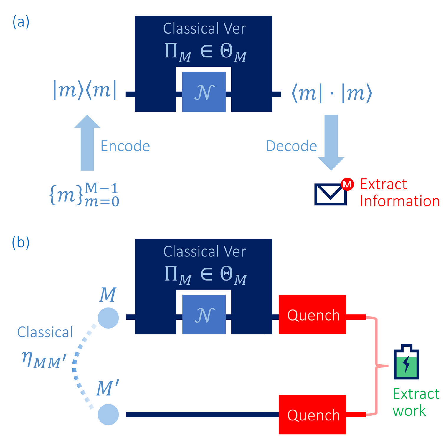
Figure 1: (a) The one-shot $\Theta$-assisted classical capacity defined in Eq. (3) describes a communication task in which the sender encodes classical information $\{m\}_{m=0}^{M-1}$ into quantum states $\{|m\rangle\}_{m=0}^{M-1}$. After transmission via $\mathcal{N}$ assisted by some $\Pi_{M}\in\Theta_{M}$, the receiver decodes the transmitted classical data by the projective measurement $\{|m\rangle\langle m|\}_{m=0}^{M-1}$. (b) The one-shot $\Theta$-assisted $\epsilon$-deterministic work extraction from the maintained correlation defined in Eq. (III) describes a task aiming to extract the highest amount of work from the bipartite classical correlation, which is carried by $\eta_{MM^{\prime}}$, maintained by locally performed classical versions of $\mathcal{N}$ assisted by $\Theta$. To do so, one needs to apply local quenches to abruptly change local Hamiltonians so that the bipartite output state after the local dynamics $\Pi_{M}(\mathcal{N})$ becomes locally thermal. Finally, one extracts work from the bipartite state. As explained in Sec. II.2, the extracted energy is guaranteed to be solely from the output state’s correlation content.

III Thermodynamic Bounds on Classical Capacity

We aim to understand the thermodynamic criterion of transmitting classical information. Following Ref. [38], our strategy is to construct bounds on the one-shot $\Theta$-assisted classical capacity by thermodynamic quantities. Such bounds can help us conclude thermodynamic conditions necessary for communicating classical information in the $\Theta$-assisted scenario. With this strategy in mind, we now introduce two thermodynamic tasks relevant to the bounds. To introduce the first task, consider the following question with a given channel $\mathcal{N}$:

What is the highest extractable work from the classical correlation maintained by $\mathcal{N}$’s classical versions?

This question can be answered operationally by the following task. Consider a state $\eta_{MM^{\prime}}$ in a bipartite system $MM^{\prime}$ with an equal local dimension (which is again denoted by $M$). Assume it is diagonal in the given computational basis $\{|m\rangle_{M}\otimes|n\rangle_{M^{\prime}}\}_{n,m=0}^{M-1}$. Then we call such a state classical, since classical probability distributions can characterize it. For a classical input $\eta_{MM^{\prime}}$, the task then demands a classical version of $\mathcal{N}$ assisted by $\Theta$ in an $M$-to-$M$ setting to locally act on half of $\eta_{MM^{\prime}}$. After that, one extracts work from the correlation of the bipartite output state. Using Åberg’s scenario and optimizing over all possible classical input $\eta_{MM^{\prime}}$, local dimensions $M$, and classical versions of $\mathcal{N}$, one obtains the following highest $\epsilon$-deterministic extractable work from the maintained classical correlation [see also Figure 1 (b)]:

$$W^{\epsilon}_{\rm corr|\Theta,(1)}(\mathcal{N})\coloneqq$$

$$\quad\quad\quad\sup_{\begin{subarray}{c}M\in\mathbb{N},\eta_{MM^{\prime}}\\ \Pi_{M}\in\Theta_{M}\end{subarray}}W_{\rm corr,(1)}^{\epsilon}\left[(\Pi_{M}(\mathcal{N})\otimes\mathcal{I}_{M^{\prime}})(\eta_{MM^{\prime}})\right].$$ (7)

The second task, on the other hand, is obtained by imposing the following three constraints on the first task: (1) initial Hamiltonians are all fully degenerate. (2) the bipartite input is always the maximally correlated classical state, which is given by $\Phi_{MM^{\prime}}=\frac{1}{M}\sum_{m=0}^{M-1}|m\rangle\langle m|_{M}\otimes|m\rangle\langle m|_{M^{\prime}}$. (3) $\left\|\Pi_{M}(\mathcal{N})\left(\frac{\mathbb{I}_{M}}{M}\right)-\frac{\mathbb{I}_{M}}{M}\right\|_{1}<2\epsilon$; namely, we are only allowed to use classical versions that are $\epsilon$-closed to Gibbs-preserving channels (i.e., channels that keep the thermal state invariant) as measured by the trace distance. This task induces the following highest extractable work from the classical correlation maintained by $\Pi_{M}(\mathcal{N})$ with some $\Pi_{M}\in\Theta_{M}$ whose ability to drive the local system out of thermal equilibrium is of the order $\sim O(\epsilon)$:

$$W_{\rm\Phi|\Theta,(1)}^{\epsilon}(\mathcal{N})\coloneqq$$

$$\sup_{\begin{subarray}{c}M\in\mathbb{N},\Pi_{M}\in\Theta_{M}\\ \left\|\Pi_{M}(\mathcal{N})\left(\frac{\mathbb{I}_{M}}{M}\right)-\frac{\mathbb{I}_{M}}{M}\right\|_{1}<2\epsilon\end{subarray}}W_{\rm corr,(1)}^{\epsilon}\left[(\Pi_{M}(\mathcal{N})\otimes\mathcal{I}_{M^{\prime}})(\Phi_{MM^{\prime}})\right].$$ (8)

It turns out that the two thermodynamic tasks that we just introduced can equivalently characterize $\Theta$-assisted classical communication.

III.1 Bounding Classical Capacity by Work Extraction

As our first main result, we report the following bounds on the one-shot $\Theta$-assisted classical capacity in terms of thermodynamic quantities defined in Eqs. (III) and (III):

Theorem 1.

(Thermodynamic Bounds on Classical Capacity)
Given a set of superchannels $\Theta$ as the allowed assistance structure and a fixed temperature $0<T<\infty$. Suppose initial Hamiltonians are fully degenerate. For a channel $\mathcal{N}$ and errors $0<\delta\leq\omega<\epsilon\leq 1-\frac{1}{\sqrt{2}}$, we have that $\displaystyle W_{\rm corr|\Theta,(1)}^{\omega}(\mathcal{N})-k_{B}T\ln\frac{4\epsilon}{(\epsilon-\omega)^{2}(1-\omega)}$ $\displaystyle\quad\quad\quad\leq(k_{B}T\ln 2)C_{\Theta,(1)}^{\epsilon}(\mathcal{N})\leq W_{\rm\Phi|\Theta,(1)}^{\epsilon+\delta}(\mathcal{N}).$ (9)

Sketch of the proof. First, we obtain upper and lower bounds on $C_{\Theta,(1)}^{\epsilon}$ in terms of entropic quantities, which are summarized in Theorem A.7. After that, we relate these upper and lower bounds to the above-mentioned thermodynamic tasks and complete the proof. The full proof is given in Appendix A, and here we focus on the implications of Theorem 1 to thermodynamics. $\square$

Since by definition $W_{\rm\Phi|\Theta,(1)}\leq W_{\rm corr|\Theta,(1)}$, Theorem 1 implies that

$W_{\rm\Phi|\Theta,(1)}\approx W_{\rm corr|\Theta,(1)}\approx C_{\Theta,(1)}$ up to one-shot error terms.

From here we learn that a broad class of classical communication scenario, as characterized by $C_{\Theta,(1)}$, are physically equivalent to work extraction tasks depicted by $W_{\rm corr|\Theta,(1)}$ and $W_{\rm\Phi|\Theta,(1)}$. This gives a quantitative correspondence between communication and thermodynamics. We will continue on discussing various implications and applications of Theorem 1 in the next section.

IV Implications and Applications

IV.1 Thermodynamic Criterion of Classical Communication

Apart from offering a quantitative bridge between thermodynamic tasks and communication scenarios, Theorem 1 also allows us to explore the physical criterion behind transmitting classical information. Following Ref. [38], Theorem 1 provides the following physical message, answering the central question that we post at the beginning of this work:

Finding. (Thermodynamic Criterion of Communication)
In the one-shot regime through the $\Theta$-assisted scenario, communicating $n$ bits of classical information (i.e., having the capacity no less than $n$) is equivalent to possessing $n\times k_{B}T\ln 2$ amounts of $\Theta$-assisted $\epsilon$-deterministic extractable work from the maintained classical correlation, up to an one-shot error term $\sim O\left(\log_{2}\frac{1}{\epsilon}\right)$.

Consequently, we identify the thermodynamic requirement behind classical communication scenarios, which is given by the extractable work from classical correlation. Theorem 1 offers the first quantitative connection between one-shot communication and the small scale thermodynamics. We comment that the upper bound is tight since all state preparation channels achieve it. In general, its attainability depends on the underlying set $\Theta$. Note that any term of the order $\sim O(\log_{2}\frac{1}{\epsilon})$ can cause vanishing contribution when we consider sufficiently many (but finite) copies of the channel and average the corresponding capacity over the number of copies. Hence, in this sense, two one-shot quantities can give the same physical meaning despite a difference of the order $\sim O(\log_{2}\frac{1}{\epsilon})$.

IV.2 Thermodynamic Criterion of Transmitting Classical Information

Theorem 1 characterizes the channel’s ability to transmit classical information when members from $\Theta$ assist it. Hence, the corresponding thermodynamic criterion also contains contributions from the assisting structure $\Theta$. To see the primal ability of a channel to transmit classical information, one needs to turn off all possible assistance. This can be done by setting $\Theta=\Theta_{\rm C}\coloneqq\{\Pi(\mathcal{N})=\mathcal{N}\;\forall\mathcal{N}\}$, i.e., the one containing only identity superchannels. In this case, the associated one-shot classical capacity measures the transmissible amounts of classical information solely through the channel; i.e., $m\mapsto{\rm tr}[E_{m}\mathcal{N}(\rho_{m})]$. The corresponding thermodynamic criterion is purely from information transmission. In this specific case, we have $W_{\rm corr|\Theta_{C},(1)}^{\epsilon}(\mathcal{N})=\sup_{M\in\mathbb{N},\eta_{MM^{\prime}},\mathcal{N}_{M}}W_{\rm corr,(1)}^{\epsilon}\left[(\mathcal{N}_{M}\otimes\mathcal{I}_{M^{\prime}})(\eta_{MM^{\prime}})\right],$ where we use the notation $\mathcal{N}_{M}\coloneqq\mathcal{E}_{{\rm de}|M}\circ\mathcal{N}\circ\mathcal{E}_{{\rm en}|M}$ to represent all possible classical versions of $\mathcal{N}$ assisted by $\Theta_{\rm C}$ in the $M$-to-$M$ setting. $\mathcal{N}_{M}$s’ can be understood as classical versions of the channel $\mathcal{N}$ itself. Consequently, $W_{\rm corr|\Theta_{C},(1)}^{\epsilon}(\mathcal{N})$ is the highest $\epsilon$-deterministic extractable work from the classical correlation maintained by any classical realization of $\mathcal{N}$. Utilizing Theorem 1, we learn that, up to an error $\sim O\left(\log_{2}\frac{1}{\epsilon}\right)$ in the one-shot regime, transmitting $n$ bits of classical information via $\mathcal{N}$ is equivalent to $n\times k_{B}T\ln 2$ extractable work from the classical correlation maintained by $\mathcal{N}$’s classical versions.

IV.3 Implications of Thermodynamics for Communication, and Implications of Communication for Thermodynamics

Now we use some examples to illustrate the flexibility and applicability of Theorem 1 in existing scenarios. First, consider $\Theta=\Theta_{\rm C}$. In this case, both upper and lower bounds reported in Theorem 1 are potentially tighter than the ones reported in Ref. [67] (see the discussion below Theorem A.8 for details). When $\Theta=\Theta_{\rm LOSE}$, the corresponding one-shot classical capacity is called entanglement-assisted, denoted by $C_{\rm EA,(1)}^{\epsilon}$ (see, e.g., Refs. [70, 72, 71]). Theorem 1 implies that, up to $O\left(\log_{2}\frac{1}{\epsilon}\right)$, $C_{\rm EA,(1)}^{\epsilon}(\mathcal{N})\approx W_{\rm corr|\Theta_{\rm LOSE},(1)}^{\epsilon}(\mathcal{N})$, which is the extractable work from the maintained classical correlation assisted by all possible LOSE superchannels. Combining with the known entropic bounds on $C_{\rm EA,(1)}^{\epsilon}$ reported in, e.g., Refs. [70, 72, 71], Theorem 1 potentially gives these entropies thermodynamic meanings in work extraction. The same argument also works when we take $\Theta=\Theta_{\rm NS}$, and the one-shot non-signaling-assisted classical capacity $C_{\rm NS,(1)}^{\epsilon}$ is related to $W_{\rm corr|\Theta_{\rm NS},(1)}^{\epsilon}(\mathcal{N})$, offering a link between thermodynamics and the entropic bounds found in, e.g., Refs. [69, 73, 74, 75, 22]. Note that there exist other thermodynamic trade-off behind classical communication. For instance, in Ref. [38] the smallest heat bath size needed to thermalize all outputs of a channel is also reported as a candidate. The advantage of Theorem 1 is the direct correspondence between classical communication scenarios and work extraction tasks which is valid for a broad range of different scenarios.

Theorem 1 also provides a route to understand thermodynamic properties through established tools in communication theory. As mentioned previously, Theorem 1 implies that the seemingly different quantities $W^{\epsilon}_{\rm corr|\Theta,(1)}$ and $W^{\epsilon}_{\rm\Phi|\Theta,(1)}$ turn out to be equivalent, up to an one-shot error term. This means the optimal performance in the work extraction task characterized by $W^{\epsilon}_{\rm corr|\Theta,(1)}$ is actually achievable by only considering maximally correlated state $\Phi_{MM^{\prime}}$ as the bipartite input and classical versions $\Pi_{M}(\mathcal{N})$ that are almost Gibbs-preserving, as the one achieving $W^{\epsilon}_{\rm\Phi|\Theta,(1)}$. In other words, Theorem 1 helps us to equate optimal solutions of different thermodynamic tasks. In fact, once we know how to estimate the classical capacity $C_{\Theta,(1)}^{\epsilon}$, then Theorem 1 provides a way to estimate the extractable works $W^{\epsilon}_{\rm corr|\Theta,(1)},W^{\epsilon}_{\rm\Phi|\Theta,(1)}$. This means communication-theoretic results can be used to to answer certain thermodynamic questions quantitatively.

IV.4 Asymptotic Regime and Thermodynamic Meaning of Holevo-Schumacher-Westmoreland Theorem

When we consider multi-copy and take the average, we can recover the asymptotic classical capacity assisted by different structures $\Theta$. Thus, Theorem 1 can also provide thermodynamic bounds in the asymptotic limit. First, we define $\Theta$-assisted classical capacity as

$$C_{\Theta}(\mathcal{N})\coloneqq\lim_{\epsilon\to 0}\varliminf_{k\to\infty}\frac{1}{k}C_{\Theta,(1)}^{\epsilon}\left(\mathcal{N}^{\otimes k}\right).$$ (10)

This notion recovers various scenarios such as the standard, entanglement-assisted, and non-signaling assisted scenarios by selecting different $\Theta$. Now, one can apply the iid limit and obtain the asymptotic version of Theorem 1:

Corollary 2.

(Thermodynamic Meaning of Classical Capacity)
Given a set of superchannels $\Theta$ as the allowed assistance structure and a fixed temperature $0<T<\infty$. Suppose initial Hamiltonians are fully degenerate. For a channel $\mathcal{N}$, we have that $\displaystyle(k_{B}T\ln 2)C_{\Theta}(\mathcal{N})=W_{\rm corr|\Theta}(\mathcal{N})=W_{\Phi|\Theta}(\mathcal{N}),$ (11) where $\displaystyle W_{\rm corr|\Theta}(\mathcal{N})$ $\displaystyle\coloneqq\lim_{\epsilon\to 0}\varliminf_{k\to\infty}\frac{1}{k}W_{\rm corr|\Theta,(1)}^{\epsilon}\left(\mathcal{N}^{\otimes k}\right);$ (12) $\displaystyle W_{\Phi|\Theta}(\mathcal{N})$ $\displaystyle\coloneqq\lim_{\epsilon\to 0}\varliminf_{k\to\infty}\frac{1}{k}W_{\Phi|\Theta,(1)}^{\epsilon}\left(\mathcal{N}^{\otimes k}\right)$ (13) can be understood as the average extractable work from the maintained correlation.

Hence, the physical message that we have obtained in the one-shot regime can directly apply to the asymptotic limit as an equality without any error term. To illustrate Corollary 2, we use the standard classical capacity as an example, and the same argument works for other choices of $\Theta$. Setting $C_{\Theta_{\rm C}}=C$, the classical capacity is then given by $C(\mathcal{N})\coloneqq\lim_{\epsilon\to 0}\varliminf_{k\to\infty}\frac{1}{k}C_{(1)}^{\epsilon}\left(\mathcal{N}^{\otimes k}\right)$ [67]. Then Corollary 2 implies that

$$(k_{B}T\ln 2)C(\mathcal{N})=W_{\rm corr|\Theta_{\rm C}}(\mathcal{N}).$$ (14)

Interestingly, Eq. (14) can be interpreted as a thermodynamic version of the famous Holevo-Schumacher-Westmoreland (HSW) Theorem [62, 63] (see also Ref. [79]). As explicitly stated in Theorem B.1, HSW Theorem equates classical capacity and the regularized version of Holevo information. Here, as a consequence of Corollary 2, we learn that the thermodynamic quantity $W_{\rm corr|\Theta_{\rm C}}$ can equally describe the classical capacity in the unit of $k_{B}T\ln 2$. Furthermore, as another implication, one can use Theorem 1 to prove HSW Theorem with Holevo information subject to thermodynamic constraints (see Theorem B.2 and Appendix B for details). These observations give HSW Theorem interpretations in thermodynamic contexts, again illustrating how Theorem 1 connects thermodynamics and communication. Finally, similar to the one-shot case, Eq. (14) tells use the following physical message:

Finding. (Asymptotic Criterion of Communication)
In the asymptotic regime, transmitting $n$ bits of classical information equals $n\times k_{B}T\ln 2$ averaged extractable work from classical correlation maintained by the channel’s classical versions.

As an important remark, we note that an early work by Plenio [46] has mentioned the connection between Holevo bound and Landauer erasure process by using the latter to argue the relation between Holevo bound and classical capacity (see also the early observations of the connection between communication and thermodynamics in Refs. [47, 48, 49]). Here we provide alternative thermodynamic interpretations, demonstrating the thermodynamic criterion necessary for information transmission.

V Detecting Channel Resource By Work Extraction

Our results provide the first thermodynamic meaning of classical capacities assisted by different $\Theta$ in both one-shot and asymptotic regimes. They suggest a close relationship between the performance in classical communication and extractable work allowed by the given channel. Since the ability to communicate information can be cast into a channel resource theory (see Appendix C.2 for a brief introduction), our findings naturally motivate us to ask:

Can work extraction detect general channel resources?

Utilizing the resource witness recently established in Refs. [39, 28], we can answer this question in the positive by using the work extraction scenario introduced by Skrzypczyk-Short-Popescu (SSP) [80]. Again, to avoid distracting from the main focus, this scenario will be detailed in Appendix C.1. Here we mention that the major difference between SSP scenario and Åberg’s scenario is that the former focuses on averaged extractable work and averaged energy conservation of the global system. In SSP scenario, with a given fixed temperature $T$, the extractable work from an arbitrary quantum state $\rho$ subject to a thermal state $\gamma_{H}$ with Hamiltonian $H$ is

$$W_{{\rm SSP}}(\rho,H)\coloneqq(k_{B}T\ln 2)S\left(\rho\,\|\,\gamma_{H}\right),$$ (15)

where $S(\rho\,\|\,\sigma)\coloneqq{\rm tr}\left[\rho\left(\log_{2}\rho-\log_{2}\sigma\right)\right]$ is the quantum relative entropy. Now, we observe that this quantity can be decomposed into two terms, governing two different sources of work extraction:

$$W_{{\rm SSP}}(\rho,H)=W_{\rm gap}(\rho,H)+W_{\rm info}(\rho),$$ (16)

where

$$W_{\rm info}(\rho)\coloneqq W_{{\rm SSP}}(\rho,0)$$ (17)

is the work extracted with the zero Hamiltonian (namely, there is no energy gap and the energy is set to zero), and

$$W_{\rm gap}(\rho,H)\coloneqq W_{{\rm SSP}}(\rho,H)-W_{{\rm SSP}}(\rho,0).$$ (18)

$W_{\rm info}(\rho)$ represents the extractable work purely from the information content of $\rho$, since it is the work extracted when we turn off energy gaps in the system Hamiltonian. On the other hand, we have a nonzero $W_{\rm gap}(\rho,H)$ if and only if the Hamiltonian’s energy gaps are turned on. Hence, $W_{\rm gap}(\rho,H)$ can be understood as the work extracted from the effect of non-vanishing energy gaps in the Hamiltonian $H$ when the system is initially prepared in the state $\rho$. It turns out that, unexpectedly, one can use this quantity to witness a broad class of channel resources. To see this, consider a given set $\mathfrak{F}$, consisting of channels from $S_{\rm in}$ to $S_{\rm out}$. Then this set characterizes a resource of channels by defining that a channel $\mathcal{E}$ possesses the resource if and only if $\mathcal{E}\notin\mathfrak{F}$. For instance, if $\mathfrak{F}$ is the set of all state preparation channels, then the corresponding resource is the ability to transmit information in non-signaling-assisted classical communication [22]. Also, if $\mathfrak{F}$ contains all entanglement-annihilating channels [81], then the ability to preserve entanglement is the underlying resource [23]. Then we have the following result:

Theorem 3.

(Channel Resource and Work Extraction)
Let $\mathfrak{F}$ be a convex and compact set of channels from $S_{\rm in}$ to $S_{\rm out}$. Then $\mathcal{E}\notin\mathfrak{F}$ if and only if for every temperature $0<T<\infty$ there exist finitely many Hamiltonians $\{H_{i}>0\}_{i}$ and states $\{\rho_{i}\}_{i}$ such that $\displaystyle\sum_{i}W_{\rm gap}\left[\mathcal{N}(\rho_{i}),H_{i}\right]>\max_{\mathcal{L}\in\mathfrak{F}}\sum_{i}W_{\rm gap}\left[\mathcal{L}(\rho_{i}),H_{i}\right].$ (19) Consequently, general channel resources can be witnessed by extractable work from energy gaps.

Sketch of the proof. First, we prove an operational characterization of an arbitrary resource carried by collections of channels in state discrimination tasks. This result, which is summarized in Theorem C.3, generalizes Theorem 2 in Ref. [39] and modifies the main theorem in Ref. [28]. We then transform the state discrimination task into a modified version of SSP work extraction scenario and use Theorem C.3 to complete the proof. Note that Theorem 3 can be extended to resources of collections of channels. Here we only focus on channels in order to simplify the presentation. See Appendix C and Theorem C.6 for details. $\square$

Schematically, Theorem 3 shows that there exists a combination of states $\rho_{i}$ and Hamiltonians $H_{i}$ such that one can use the extractable work from the energy gaps of $\mathcal{N}(\rho_{i})$ subject to $H_{i}$, averaged over $i$, to witness the resourcefulness of $\mathcal{N}$. In other words, no free channel can outperform this averaged extractable work from energy gaps. It is worth mentioning that the currently known operational tasks that can detect general channel resources are state discrimination tasks [14, 15, 16, 17, 26, 11, 39, 42], parameter estimation tasks [35], and exclusion tasks [28, 27]. It is still unknown whether there is any thermodynamic task that can achieve the same goal for general channel resources, and Theorem 3 answers this question in the positive.

VI Conclusion

This work aims to seek a thermodynamic criterion for a quantum channel to transmit classical information. Utilizing the tools established in quantum communication, quantum thermodynamics, and dynamical resource theory, we answer this question by providing thermodynamic upper and lower bounds on the one-shot classical capacity that is assisted by an arbitrarily given set of superchannels. The physical meaning of the bounds is the optimal extractable work from the classical correlation maintained by the channel. Our results imply that transmitting $n$ bits of classical information is equivalent to having this extractable work equal $n\times k_{B}T\ln 2$. This physical message depicts the thermodynamic criterion that a channel must fulfill to transmit classical information.

Our results apply to several known scenarios, building up connections between communication and thermodynamics. Furthermore, the same physical finding can be extended to the asymptotic regime, giving the well-known Holevo-Schumacher-Westmoreland Theorem thermodynamic meanings in different work extraction tasks.

Finally, we continue investigating the connection between work extraction and the general resource theory of channels. We show that the extractable work from energy gaps can witness a broad class of channel resources. This result not only establishes the first thermodynamic witness for general resource theories, but also reveals an application of using energy gaps to detect resourcefulness in dynamics.

Many open questions remain, and here we list a few. First, it is still unknown whether one can improve the bound or even extract special thermodynamic meanings by considering a specific set of superchannels in Theorem 1. Furthermore, several recent results have addressed the thermodynamic cost of encoding classical information into a state [18, 13, 33]. This is related to the carriable amount of classical information under thermodynamic restrictions of a state. On the other hand, in this work, we study the thermodynamic criterion of information transmission via a channel. Hence, despite the conceptual difference between our findings and Refs. [18, 13, 33], it is rewarding to explore the connection and relation between these two approaches. Finally, inspired by a recent work studying thermal operation subject to non-ideal baths with fluctuation [82], it is also interesting to discuss how robust our results can be when noises and fluctuation occur.

We hope that our results can initiate people’s interest in the interplay of communication, thermodynamics, and dynamical resource theory.

Appendix A Formal Form and Detailed Proof of Theorem 1

In this Appendix, we will present a formal proof of Theorem 1. We start with formalizing definitions of notations in Sec. A.1. Then, in Sec. A.2, we will prove upper and lower bounds in terms of the $\epsilon$-smoothed relative Rényi $0$-entropy [77]. In Sec. A.3 we briefly review work extraction scenario introduced in Ref. [77]. Finally, in Sec. A.4 we prove Theorem 1.

A.1 Definitions, Terminologies, and Preliminary Lemmas

To make our consideration rigorous, let us define the following notations. First, throughout this Appendix, we will use the symbol $M$ (and, in some limited cases, $L$) to denote the size of classical messages. It can be given by the dimension of a system spanned by a pre-defined orthonormal basis $\{|m\rangle\}_{m=0}^{M-1}$. When we only consider states diagonal in this given basis, i.e., states of the form $\sum_{m=0}^{M-1}p_{m}|m\rangle\langle m|$, then all of them can be equivalently described by a classical probability distribution $\{p_{m}\}_{m=0}^{M-1}$. Due to this reason, we call such a system a classical system. For a classical system with dimension $M$, we again use the symbol $M$ to denote the system. Note that when we say a system $M$ is classical, then it is understood that an orthonormal basis $\{|m\rangle\}_{m=0}^{M-1}$ has been assigned. This notion helps us to define classical behaviors of a quantum channel through the following terminology:

Definition A.1.

(Classical-to-Quantum and Quantum-to-Classical Channels)

• ${\rm CQ}_{M\to S}$ denotes the set of all classical-to-quantum channels from a classical system $M$ to a system $S$ of the form

  $$\sum_{m=0}^{M-1}\rho_{m|S}\langle m|(\cdot)_{M}|m\rangle_{M},$$ (20)

  where $\{\rho_{m|S}\}_{m=0}^{M-1}$ are states in $S$.

• ${\rm QC}_{S\to M}$ denotes the set of all quantum-to-classical channels from a system $S$ to a classical system $M$ of the form

  $$\sum_{m=0}^{M-1}|m\rangle\langle m|_{M}{\rm tr}[E_{m|S}(\cdot)_{S}],$$ (21)

  where $\{E_{m|S}\}_{m=0}^{M-1}$ is a POVM in $S$.

A channel is further called a classical-to-classical channel in a classical system $M$, or simply a $M$-to-$M$ classical channel, if it can be written as $\mathcal{L}\circ\mathcal{K}$ for some classical-to-quantum channel $\mathcal{K}\in{\rm CQ}_{M\to S}$ and quantum-to-classical channel $\mathcal{L}\in{\rm QC}_{S\to M}$.

With the above terminologies, the channel $\mathcal{E}_{{\rm en}|M}:M\to S_{\rm in}$ in the main text is a member of ${\rm CQ}_{M\to S_{\rm in}}$; similarly, $\mathcal{E}_{{\rm de}|M}:S_{\rm out}\to M$ is in ${\rm QC}_{S_{\rm out}\to M}$. Furthermore, it allows us to formally define the classical versions of the set $\Theta$, the term that has been used in Eq. (2) in the main text:

Definition A.2.

(Classical Versions of Superchannels)

Given a set of superchannels $\Theta$ and a classical system $M$. Then the set of $M$-to-$M$ classical versions of $\Theta$, denoted by the set $\Theta_{M}$, is defined by

$$\Theta_{M}\coloneqq\left\{\mathcal{L}\circ[\Pi(\cdot)]\circ\mathcal{K}\,\middle|\,\Pi\in\Theta,\mathcal{K}\in{\rm CQ}_{M\to S_{\rm in|\Pi}},\mathcal{L}\in{\rm QC}_{S_{\rm out|\Pi}\to M}\right\},$$ (22)

where $S_{\rm in|\Pi},S_{\rm out|\Pi}$ are the input and output spaces of the output channel of $\Pi$.

This set characterizes all possible classical-to-classical realizations induced by $\Theta$ in a $M$-dimensional setting. Hence, every element $\Pi_{M}\in\Theta_{M}$ maps a quantum channel to some $M$-to-$M$ classical channel. Now we define the one-shot $\Theta$-assisted classical capacity as follows:

Definition A.3.

(One-Shot $\Theta$-Assisted Classical Capacity)

For a given set of superchannels $\Theta$ and an error $0\leq\epsilon\leq 1$, the one-shot $\Theta$-assisted classical capacity subject to an error $\epsilon$ of a given channel $\mathcal{N}$ is defined by

$$C_{\Theta,(1)}^{\epsilon}(\mathcal{N})\coloneqq\max\left\{\log_{2}M\,\middle|\,\exists\Pi\in\Theta,{\rm states}\;\{\rho_{m}\}_{m=0}^{M-1},{\rm POVM}\;\{E_{m}\}_{m=0}^{M-1}\;{\rm s.t.}\;\sum_{m=0}^{M-1}\frac{1}{M}{\rm tr}\left[E_{m}\Pi(\mathcal{N})(\rho_{m})\right]\geq 1-\epsilon\right\}.$$ (23)

One motivation to study the one-shot classical capacity is that, as mentioned in Ref. [67], it provides richer knowledge compared with the asymptotic classical capacity; that is, applying multi-copy limit will reproduce the asymptotic result. Using the previously introduced terminologies, Definition A.3 can be rewritten in an alternative form as follows:

Fact A.4.

(Alternative Form of One-Shot $\Theta$-Assisted Classical Capacity)

Based on the same setting as in Definition A.3, we have that

$$C_{\Theta,(1)}^{\epsilon}(\mathcal{N})=\max\{\log_{2}M\,|\,\exists\Pi_{M}\in\Theta_{M}\;{\rm s.t.}\;P_{s}[\Pi_{M}(\mathcal{N})]\geq 1-\epsilon\},$$ (24)

where

$$P_{s}[\Pi_{M}(\mathcal{N})]\coloneqq\sum_{m=0}^{M-1}\frac{1}{M}\langle m|\Pi_{M}(\mathcal{N})(|m\rangle\langle m|)|m\rangle$$ (25)

is the average success probability of the $M$-to-$M$ classical channel $\Pi_{M}(\mathcal{N})$.

Proof.

As explained in the main text, the validity of Eq. (24) can be seen by noting that

• For every set of states $\{\rho_{m|S}\}_{m=0}^{M-1}$ in $S$, there exists a channel $\mathcal{K}_{M\to S}\in{\rm CQ}_{M\to S}$ given by Eq. (20) such that

  $$\mathcal{E}(\rho_{m})=\mathcal{E}\circ\mathcal{K}_{M\to S}(|m\rangle\langle m|)$$ (26)

  for every index $m$ and channel $\mathcal{E}$.

• For every POVM $\{E_{m|S}\}_{m=0}^{M-1}$ in $S$, there exists a channel $\mathcal{L}_{S\to M}\in{\rm QC}_{S\to M}$ given by Eq. (21) such that

  $${\rm tr}\left(E_{m|S}\rho\right)=\langle m|\mathcal{L}_{S\to M}(\rho)|m\rangle$$ (27)

  for every index $m$ and state $\rho$.

Consequently, from Definition A.3, we have that (let $S_{\rm in|\Pi},S_{\rm out|\Pi}$ be the input and output spaces of the output channel of $\Pi$)

$$C_{\Theta,(1)}^{\epsilon}(\mathcal{N}_{S})=\max\left\{\log_{2}M\,\middle|\,\exists\Pi\in\Theta,\mathcal{K}\in{\rm CQ}_{M\to S_{\rm in|\Pi}},\mathcal{L}\in{\rm QC}_{S_{\rm out|\Pi}\to M}\;{\rm s.t.}\;P_{s}[\mathcal{L}\circ\Pi(\mathcal{N})\circ\mathcal{K}]\geq 1-\epsilon\right\},$$ (28)

and the claim follows by using Definition A.2. ∎

A simple yet important observation is that if we set $\Theta=\Theta_{\rm C}\coloneqq\{(\cdot)\mapsto(\cdot)\}$; that is, it only contains identity superchannel, then we have $C_{\Theta_{\rm C},(1)}^{\epsilon}=C_{(1)}^{\epsilon}$, which is the (standard) one-shot classical capacity [67]. As mentioned in the main text, this quantity measures the channel’s primal ability to transmit classical information in the one-shot regime, and every $\Theta$-assisted scenario should be linked to this fundamental case. This can be seen by the following observation:

Fact A.5.

(Standard Classical Capacity Representation of $\Theta$-Assisted Capacity)

For a given set of superchannels $\Theta$, a channel $\mathcal{N}$, and an error $0\leq\epsilon\leq 1$, we have that

$$C_{\Theta,(1)}^{\epsilon}(\mathcal{N})=\sup_{\Pi\in\Theta}C_{(1)}^{\epsilon}[\Pi(\mathcal{N})].$$ (29)

Proof.

Using Fact A.4, we can write down

$$\sup_{\Pi\in\Theta}C_{(1)}^{\epsilon}[\Pi(\mathcal{N})] \coloneqq\sup_{\Pi\in\Theta}\max\left\{\log_{2}M\,\middle|\,\exists\mathcal{K}\in{\rm CQ}_{M\to S_{\rm in|\Pi}},\mathcal{L}\in{\rm QC}_{S_{\rm out|\Pi}\to M}\;{\rm s.t.}\;P_{s}[\mathcal{L}\circ\Pi(\mathcal{N})\circ\mathcal{K}]\geq 1-\epsilon\right\}$$

$$=\max\{\log_{2}M\,|\,\exists\Pi_{M}\in\Theta_{M}\;{\rm s.t.}\;P_{s}[\Pi_{M}(\mathcal{N})]\geq 1-\epsilon\}=C_{\Theta,(1)}^{\epsilon}(\mathcal{N}).$$ (30)

∎

Finally, we note the following observation:

Fact A.6.

(Preserving the Gibbs-Preserving Property)

Given a set of superchannels $\Theta$, a channel $\mathcal{N}$, and an error $0\leq\epsilon\leq 1$. Then for every $\Pi_{M}\in\Theta_{M}$ satisfying $P_{s}[\Pi_{M}(\mathcal{N})]\geq 1-\epsilon$ we have that

$$\left\|\Pi_{M}(\mathcal{N})\left(\frac{\mathbb{I}_{M}}{M}\right)-\frac{\mathbb{I}_{M}}{M}\right\|_{1}\leq 2\epsilon.$$ (31)

In other words, when the system Hamiltonian is fully degenerate, $\Pi_{M}$ maps the channel $\mathcal{N}$ to some output channel that is closed to a Gibbs-preserving channel, up to an error $\epsilon$ measure by the trace distance.

Proof.

For such a $\Pi_{M}\in\Theta_{M}$, direct computation shows that

$$\left\|\Pi_{M}(\mathcal{N})\left(\frac{\mathbb{I}_{M}}{M}\right)-\frac{\mathbb{I}_{M}}{M}\right\|_{1} =\left\|\frac{1}{M}\sum_{n=0}^{M-1}\left[\sum_{m=0}^{M-1}\langle n|\Pi_{M}(\mathcal{N})(|m\rangle\langle m|)|n\rangle-1\right]|n\rangle\langle n|\right\|_{1}$$

$$=\left\|\frac{1}{M}\sum_{n=0}^{M-1}\left[\left(\langle n|\Pi_{M}(\mathcal{N})(|n\rangle\langle n|)|n\rangle-1\right)+\sum_{\begin{subarray}{c}m=0\\ m\neq n\end{subarray}}^{M-1}\langle n|\Pi_{M}(\mathcal{N})(|m\rangle\langle m|)|n\rangle\right]|n\rangle\langle n|\right\|_{1}$$

$$=\frac{1}{M}\sum_{n=0}^{M-1}\left|\left(\langle n|\Pi_{M}(\mathcal{N})(|n\rangle\langle n|)|n\rangle-1\right)+\sum_{\begin{subarray}{c}m=0\\ m\neq n\end{subarray}}^{M-1}\langle n|\Pi_{M}(\mathcal{N})(|m\rangle\langle m|)|n\rangle\right|$$

$$\leq\frac{1}{M}\sum_{n=0}^{M-1}\left[\left|\langle n|\Pi_{M}(\mathcal{N})(|n\rangle\langle n|)|n\rangle-1\right|+\sum_{\begin{subarray}{c}m=0\\ m\neq n\end{subarray}}^{M-1}\langle n|\Pi_{M}(\mathcal{N})(|m\rangle\langle m|)|n\rangle\right]$$

$$=2\left(1-\frac{1}{M}\sum_{n=0}^{M-1}\langle n|\Pi_{M}(\mathcal{N})(|n\rangle\langle n|)|n\rangle\right)=2\left(1-P_{s}[\Pi_{M}(\mathcal{N})]\right)\leq 2\epsilon.$$ (32)

In the first line, we have used the fact that the output of $\Pi_{M}(\mathcal{N})$ is diagonal in the basis $\{|m\rangle\}_{m=0}^{M-1}$. ∎

A.2 One-Shot $\Theta$-Assisted Classical Capacity and Smoothed Relative Rényi $0$-Entropy

To prove Theorem 1 in the main text, we first show upper and lower bounds on $\Theta$-assisted one-shot classical capacity in terms of the following two entropies, which are closely related to each other. The first one is the $\epsilon$-smoothed relative Rényi $0$-entropy (see Supplementary Definition 6 in Ref. [77]) defined for two commuting states $\eta=\sum_{j}q_{j}|j\rangle\langle j|,\gamma=\sum_{j}r_{j}|j\rangle\langle j|$ as

$$D_{0}^{\delta}(\eta\,\|\,\gamma)\coloneqq\max_{\Lambda:\sum_{j\in\Lambda}q_{j}>1-\delta}\log_{2}\frac{1}{\sum_{j\in\Lambda}r_{j}},$$ (33)

where the maximization is taken over every possible index set $\Lambda$ satisfying the strict inequality $\sum_{j\in\Lambda}q_{j}>1-\delta$. This entropy can be extended to the hypothesis testing relative entropy with error $\epsilon$, which is defined as follows for two states $\rho,\sigma$ [67]:

$$D_{h}^{\epsilon}(\rho\,\|\,\sigma)\coloneqq\max_{\begin{subarray}{c}0\leq Q\leq\mathbb{I}\\ {\rm tr}(Q\rho)\geq 1-\epsilon\end{subarray}}\log_{2}\frac{1}{{\rm tr}(Q\sigma)}.$$ (34)

Note that in this work we use the lower case for the subscript “$h$” rather than the conventional upper case to avoid confusion with the notation of Hamiltonians “$H$.” As a direct observation from the definition Eq. (33), one can see that $D_{0}^{\epsilon}(\rho\,\|\,\sigma)\leq D_{h}^{\epsilon}(\rho\,\|\,\sigma)$ whenever they are both well-defined.

Now we are in the position to introduce the first main result in this Appendix. In what follows, we always use the symbol $M^{\prime}$ to denote an ancillary classical system $M^{\prime}$ satisfying $M^{\prime}\simeq M$. Also, $S^{\prime}$ denotes an ancillary quantum system.

Theorem A.7.

(Bounding One-Shot $\Theta$-Assisted Classical Capacity)

Given a set of superchannels $\Theta$, a channel $\mathcal{N}$, and errors $0<\delta\leq\omega<\epsilon\leq\frac{1}{2}$, we have that

$$\sup_{\begin{subarray}{c}M\in\mathbb{N},\Pi\in\Theta\\ \eta_{S_{\rm in|\Pi}S^{\prime}}=\sum_{x=0}^{M-1}p_{x}\sigma_{x|S_{\rm in|\Pi}}\otimes\kappa_{x|S^{\prime}}\end{subarray}}D_{h}^{\omega}\left[(\Pi(\mathcal{N})\otimes\mathcal{I}_{S^{\prime}})(\eta_{S_{\rm in|\Pi}S^{\prime}})\,\middle\|\,\Pi(\mathcal{N})\left(\eta_{S_{\rm in|\Pi}}\right)\otimes\eta_{S^{\prime}}\right]-\log_{2}\frac{4\epsilon}{(\epsilon-\omega)^{2}}\leq$$

$$\quad\quad\quad\quad\quad\quad C_{\Theta,(1)}^{\epsilon}(\mathcal{N})\leq\sup_{\begin{subarray}{c}M\in\mathbb{N},\Pi_{M}\in\Theta_{M}\\ \left\|\Pi_{M}(\mathcal{N})\left(\frac{\mathbb{I}_{M}}{M}\right)-\frac{\mathbb{I}_{M}}{M}\right\|_{1}\leq 2(\epsilon+\delta)\end{subarray}}D_{0}^{\epsilon+\delta}\left[(\Pi_{M}(\mathcal{N})\otimes\mathcal{I}_{M^{\prime}})(\Phi_{MM^{\prime}})\,\middle\|\,\Pi_{M}(\mathcal{N})\left(\frac{\mathbb{I}_{M}}{M}\right)\otimes\frac{\mathbb{I}_{M^{\prime}}}{M}\right],$$ (35)

where $S^{\prime}$ is some finite dimensional ancillary system which is not necessary of the same size with $S_{\rm in|\Pi}$, $\eta_{S_{\rm in|\Pi}S^{\prime}}$ is a separable state in $S_{\rm in|\Pi}S^{\prime}$ that can be written as a convex combination of $M$ product states (i.e., both $\sigma_{x|S_{\rm in|\Pi}}$, $\kappa_{x|S^{\prime}}$ are states), and $\Phi_{MM^{\prime}}\coloneqq\frac{1}{M}\sum_{m=0}^{M-1}|m\rangle\langle m|_{M}\otimes|m\rangle\langle m|_{M^{\prime}}$ is the maximally (classically) correlated state diagonal in the bipartite basis associated with the classical systems $M,M^{\prime}$.

Note that by our setting, the states $[\Pi_{M}(\mathcal{N})\otimes\mathcal{I}_{M^{\prime}}](\Phi_{MM^{\prime}})$ and $\Pi_{M}(\mathcal{N})\left(\frac{\mathbb{I}_{M}}{M}\right)\otimes\frac{\mathbb{I}_{M^{\prime}}}{M}$ are indeed simultaneously diagonalizable, meaning that the smoothed relative Rényi $0$-entropy is well-defined here. Importantly, the upper bound in the second line is further upper bounded by the lower bound in the first line, up to the one-shot error term $-\log_{2}\frac{4\epsilon}{(\epsilon-\omega)^{2}}$. This illustrates that both the upper and lower bounds will converge to the same quantity in the asymptotic limit. We choose this way to present the result to show the tightest form explicitly. Soon we will illustrate how to obtain Theorem 1 in the main text.

As the first observation, suppose the statement holds for the one-shot (standard) classical capacity $C_{(1)}$. Then Fact A.5 implies that

$$C_{\Theta,(1)}^{\epsilon}(\mathcal{N}) =\sup_{\Pi\in\Theta}C_{(1)}^{\epsilon}[\Pi(\mathcal{N})]$$

$$\leq\sup_{\Pi\in\Theta}\sup_{\begin{subarray}{c}M\in\mathbb{N}\\ \mathcal{K}\in{\rm CQ}_{M\to S_{\rm in|\Pi}},\\ \mathcal{L}\in{\rm QC}_{S_{\rm out|\Pi}\to M},\\ \left\|\mathcal{L}\circ\Pi(\mathcal{N})\circ\mathcal{K}\left(\frac{\mathbb{I}_{M}}{M}\right)-\frac{\mathbb{I}_{M}}{M}\right\|_{1}\leq 2(\epsilon+\delta)\end{subarray}}D_{0}^{\epsilon+\delta}\left[((\mathcal{L}\circ\Pi(\mathcal{N})\circ\mathcal{K})\otimes\mathcal{I}_{M^{\prime}})(\Phi_{MM^{\prime}})\,\middle\|\,(\mathcal{L}\circ\Pi(\mathcal{N})\circ\mathcal{K})\left(\frac{\mathbb{I}_{M}}{M}\right)\otimes\frac{\mathbb{I}_{M^{\prime}}}{M}\right]$$

$$\leq\sup_{\begin{subarray}{c}M\in\mathbb{N},\Pi_{M}\in\Theta_{M}\\ \left\|\Pi_{M}(\mathcal{N})\left(\frac{\mathbb{I}_{M}}{M}\right)-\frac{\mathbb{I}_{M}}{M}\right\|_{1}\leq 2(\epsilon+\delta)\end{subarray}}D_{0}^{\epsilon+\delta}\left[(\Pi_{M}(\mathcal{N})\otimes\mathcal{I}_{M^{\prime}})(\Phi_{MM^{\prime}})\,\middle\|\,\Pi_{M}(\mathcal{N})\left(\frac{\mathbb{I}_{M}}{M}\right)\otimes\frac{\mathbb{I}_{M^{\prime}}}{M}\right].$$ (36)

On the other hand, the lower bound can be rewritten as

$$\sup_{\Pi\in\Theta}\sup_{M\in\mathbb{N},\eta_{S_{\rm in|\Pi}S^{\prime}}}D_{h}^{\omega}\left[(\Pi(\mathcal{N})\otimes\mathcal{I}_{S^{\prime}})(\eta_{S_{\rm in|\Pi}S^{\prime}})\,\middle\|\,\Pi(\mathcal{N})\left(\eta_{S_{\rm in|\Pi}}\right)\otimes\eta_{S^{\prime}}\right]-\log_{2}\frac{4\epsilon}{(\epsilon-\omega)^{2}}\leq\sup_{\Pi\in\Theta}C_{(1)}^{\epsilon}[\Pi(\mathcal{N})]=C_{\Theta,(1)}^{\epsilon}(\mathcal{N}),$$ (37)

where we have used Fact A.5 again. Hence, it suffices to prove the case for the standard scenario with $C_{(1)}$. To this end, we single out this special case as the following theorem, whose validity implies Theorem A.7. In what follows, $S^{\prime}$ again denotes an ancillary quantum system, and $S_{\rm in|\mathcal{N}},S_{\rm out|\mathcal{N}}$ are the input and output systems of the given channel $\mathcal{N}$, respectively.

Theorem A.8.

(Bounding One-Shot Classical Capacity)

Given a channel $\mathcal{N}$ and errors $0<\delta\leq\omega<\epsilon\leq\frac{1}{2}$, we have that

$$\sup_{\begin{subarray}{c}M\in\mathbb{N}\\ \eta_{S_{\rm in|\mathcal{N}}S^{\prime}}=\sum_{x=0}^{M-1}p_{x}\sigma_{x|S_{\rm in|\mathcal{N}}}\otimes\kappa_{x|S^{\prime}}\end{subarray}}D_{h}^{\omega}\left[(\mathcal{N}\otimes\mathcal{I}_{S^{\prime}})(\eta_{S_{\rm in|\mathcal{N}}S^{\prime}})\,\middle\|\,\mathcal{N}\left(\eta_{S_{\rm in|\mathcal{N}}}\right)\otimes\eta_{S^{\prime}}\right]-\log_{2}\frac{4\epsilon}{(\epsilon-\omega)^{2}}\leq$$

$$\quad\quad\quad\quad\quad\quad C_{(1)}^{\epsilon}(\mathcal{N})\leq\sup_{\begin{subarray}{c}M\in\mathbb{N}\\ \mathcal{K}\in{\rm CQ}_{M\to S_{\rm in|\mathcal{N}}}\\ \mathcal{L}\in{\rm QC}_{S_{\rm out|\mathcal{N}}\to M}\\ \left\|\mathcal{L}\circ\mathcal{N}\circ\mathcal{K}\left(\frac{\mathbb{I}_{M}}{M}\right)-\frac{\mathbb{I}_{M}}{M}\right\|_{1}\leq 2(\epsilon+\delta)\end{subarray}}D_{0}^{\epsilon+\delta}\left[((\mathcal{L}\circ\mathcal{N}\circ\mathcal{K})\otimes\mathcal{I}_{M^{\prime}})(\Phi_{MM^{\prime}})\,\middle\|\,(\mathcal{L}\circ\mathcal{N}\circ\mathcal{K})\left(\frac{\mathbb{I}_{M}}{M}\right)\otimes\frac{\mathbb{I}_{M^{\prime}}}{M}\right].$$ (38)

Before the proof, we make the following important remark. The hypothesis testing bounds on the one-shot classical capacity have been reported in Ref. [67], so we must compare Theorem A.8 and the known bounds. First, for the upper bound, we learn from the definition Eq. (33) that $D_{0}^{\epsilon}(\rho\,\|\,\sigma)\leq D_{h}^{\epsilon}(\rho\,\|\,\sigma)$ whenever they are both well-defined. This means that Theorem A.8 implies the upper bound proved in Ref. [67]. On the other hand, the lower bound found in Ref. [67] is optimizing over every quantum-classical state of the form $\sigma_{S_{\rm in|\mathcal{N}}M}=\sum_{m=0}^{M-1}p_{m}\rho_{m}\otimes|m\rangle\langle m|_{M}.$ This means Theorem A.8 also implies the lower bound established in Ref. [67]. Moreover, Theorem A.7 generalizes the result found in Ref. [67] by extending it to an arbitrary $\Theta$-assisted scenario as well as providing potentially tighter bounds.

Proof.

We split the proof into two parts. First, we will show the upper bound. Then, following the approach of Ref. [67], a lower bound can be further obtained.

Proof of the Upper Bound.– By definition, we can write $C_{(1)}^{\epsilon}(\mathcal{N})$ as the following maximization

$$\begin{aligned} \max_{M,\mathcal{K},\mathcal{L}}\quad&\log_{2}M\\ {\rm s.t.}\quad&\frac{1}{M}\sum_{m=0}^{M-1}\langle m|(\mathcal{L}\circ\mathcal{N}\circ\mathcal{K})(|m\rangle\langle m|)|m\rangle\geq 1-\epsilon;\\ &\mathcal{K}\in{\rm CQ}_{M\to S_{\rm in|\mathcal{N}}};\mathcal{L}\in{\rm QC}_{S_{\rm out|\mathcal{N}}\to M};M\in\mathbb{N}.\end{aligned}$$ (39)

Using Fact. A.6, we learn that the above optimization is invariant if we add the additional constraint $\left\|\mathcal{L}\circ\mathcal{N}\circ\mathcal{K}\left(\frac{\mathbb{I}_{M}}{M}\right)-\frac{\mathbb{I}_{M}}{M}\right\|_{1}\leq 2\epsilon$, which reads

$$\begin{aligned} \max_{M,\mathcal{K},\mathcal{L}}\quad&\log_{2}M\\ {\rm s.t.}\quad&\frac{1}{M}\sum_{m=0}^{M-1}\langle m|(\mathcal{L}\circ\mathcal{N}\circ\mathcal{K})(|m\rangle\langle m|)|m\rangle\geq 1-\epsilon;\\ &\left\|\mathcal{L}\circ\mathcal{N}\circ\mathcal{K}\left(\frac{\mathbb{I}_{M}}{M}\right)-\frac{\mathbb{I}_{M}}{M}\right\|_{1}\leq 2\epsilon;\\ &\mathcal{K}\in{\rm CQ}_{M\to S_{\rm in|\mathcal{N}}};\mathcal{L}\in{\rm QC}_{S_{\rm out|\mathcal{N}}\to M};M\in\mathbb{N}.\end{aligned}$$ (40)

Now, one can observe that

$${\rm tr}\left[\left(M\Phi_{MM^{\prime}}\right)\left((\mathcal{L}\circ\mathcal{N}\circ\mathcal{K})\otimes\mathcal{I}_{M^{\prime}}\right)\left(\Phi_{MM^{\prime}}\right)\right] =\frac{1}{M}{\rm tr}\left[\sum_{n=0}^{M-1}|n\rangle\langle n|_{M}\otimes|n\rangle\langle n|_{M^{\prime}}\sum_{m=0}^{M-1}(\mathcal{L}\circ\mathcal{N}\circ\mathcal{K})(|m\rangle\langle m|_{M})\otimes|m\rangle\langle m|_{M^{\prime}}\right]$$

$$=\frac{1}{M}\sum_{m=0}^{M-1}\langle m|(\mathcal{L}\circ\mathcal{N}\circ\mathcal{K})(|m\rangle\langle m|)|m\rangle.$$ (41)

On the other hand,

$${\rm tr}\left\{\left(M\Phi_{MM^{\prime}}\right)\left[(\mathcal{L}\circ\mathcal{N}\circ\mathcal{K})\left(\frac{\mathbb{I}_{M}}{M}\right)\otimes\frac{\mathbb{I}_{M^{\prime}}}{M}\right]\right\} ={\rm tr}\left\{\sum_{m=0}^{M-1}|m\rangle\langle m|_{M}\otimes|m\rangle\langle m|_{M^{\prime}}\left[(\mathcal{L}\circ\mathcal{N}\circ\mathcal{K})\left(\frac{\mathbb{I}_{M}}{M}\right)\otimes\frac{\mathbb{I}_{M^{\prime}}}{M}\right]\right\}$$

$$=\frac{1}{M}{\rm tr}\left\{\sum_{m=0}^{M-1}|m\rangle\langle m|_{M}\left[(\mathcal{L}\circ\mathcal{N}\circ\mathcal{K})\left(\frac{\mathbb{I}_{M}}{M}\right)\right]\right\}=\frac{1}{M},$$ (42)

where we have used the fact that $\sum_{m=0}^{M-1}|m\rangle\langle m|_{M}=\mathbb{I}_{M}$ is the identity operator in the classical system $M$. Then the optimization Eq. (40) can be rewritten as follows

$$\begin{aligned} \max_{M,\mathcal{K},\mathcal{L}}\quad&\log_{2}\frac{1}{{\rm tr}\left\{\left(M\Phi_{MM^{\prime}}\right)\left[(\mathcal{L}\circ\mathcal{N}\circ\mathcal{K})\left(\frac{\mathbb{I}_{M}}{M}\right)\otimes\frac{\mathbb{I}_{M^{\prime}}}{M}\right]\right\}}\\ {\rm s.t.}\quad&{\rm tr}\left[\left(M\Phi_{MM^{\prime}}\right)\left((\mathcal{L}\circ\mathcal{N}\circ\mathcal{K})\otimes\mathcal{I}_{M^{\prime}}\right)\left(\Phi_{MM^{\prime}}\right)\right]\geq 1-\epsilon;\\ &\left\|\mathcal{L}\circ\mathcal{N}\circ\mathcal{K}\left(\frac{\mathbb{I}_{M}}{M}\right)-\frac{\mathbb{I}_{M}}{M}\right\|_{1}\leq 2\epsilon;\\ &\mathcal{K}\in{\rm CQ}_{M\to S_{\rm in|\mathcal{N}}};\mathcal{L}\in{\rm QC}_{S_{\rm out|\mathcal{N}}\to M};M\in\mathbb{N}.\end{aligned}$$ (43)

Now, based on our setting, $\mathcal{L}\circ\mathcal{N}\circ\mathcal{K}$ is a $M$-to-$M$ classical channel. This means the states $\left((\mathcal{L}\circ\mathcal{N}\circ\mathcal{K})\otimes\mathcal{I}_{M^{\prime}}\right)\left(\Phi_{MM^{\prime}}\right)$ and $(\mathcal{L}\circ\mathcal{N}\circ\mathcal{K})\left(\frac{\mathbb{I}_{M}}{M}\right)\otimes\frac{\mathbb{I}_{M^{\prime}}}{M}$ are both diagonal in the basis $\{|n\rangle_{M}\otimes|m\rangle_{M^{\prime}}\}_{n,m=0}^{M-1}$. In other words, one can write

$$\left((\mathcal{L}\circ\mathcal{N}\circ\mathcal{K})\otimes\mathcal{I}_{M^{\prime}}\right)\left(\Phi_{MM^{\prime}}\right)=\sum_{n,m}q_{(n,m)}|n\rangle\langle n|_{M}\otimes|m\rangle\langle m|_{M^{\prime}};$$ (44)

$$(\mathcal{L}\circ\mathcal{N}\circ\mathcal{K})\left(\frac{\mathbb{I}_{M}}{M}\right)\otimes\frac{\mathbb{I}_{M^{\prime}}}{M}=\sum_{n,m}r_{(n,m)}|n\rangle\langle n|_{M}\otimes|m\rangle\langle m|_{M^{\prime}},$$ (45)

where the weights $q_{(n,m)},r_{(n,m)}$ are given by

$$q_{(n,m)}\coloneqq\langle n|_{M}\otimes\langle m|_{M^{\prime}}\left((\mathcal{L}\circ\mathcal{N}\circ\mathcal{K})\otimes\mathcal{I}_{M^{\prime}}\right)\left(\Phi_{MM^{\prime}}\right)|n\rangle_{M}\otimes|m\rangle_{M^{\prime}};$$ (46)

$$r_{(n,m)}\coloneqq\langle n|_{M}\otimes\langle m|_{M^{\prime}}\left[(\mathcal{L}\circ\mathcal{N}\circ\mathcal{K})\left(\frac{\mathbb{I}_{M}}{M}\right)\otimes\frac{\mathbb{I}_{M^{\prime}}}{M}\right]|n\rangle_{M}\otimes|m\rangle_{M^{\prime}}.$$ (47)

Then Eq. (43) can be rewritten as

$$\begin{aligned} \max_{M,\mathcal{K},\mathcal{L}}\quad&\log_{2}\frac{1}{\sum_{n=m}r_{(n,m)}}\\ {\rm s.t.}\quad&\sum_{n=m}q_{(n,m)}\geq 1-\epsilon;\\ &\left\|\mathcal{L}\circ\mathcal{N}\circ\mathcal{K}\left(\frac{\mathbb{I}_{M}}{M}\right)-\frac{\mathbb{I}_{M}}{M}\right\|_{1}\leq 2\epsilon;\\ &\mathcal{K}\in{\rm CQ}_{M\to S_{\rm in|\mathcal{N}}};\mathcal{L}\in{\rm QC}_{S_{\rm out|\mathcal{N}}\to M};M\in\mathbb{N},\end{aligned}$$ (48)

which is upper bounded by

$$\begin{aligned} \max_{M,\mathcal{K},\mathcal{L},\Lambda}\quad&\log_{2}\frac{1}{\sum_{(n,m)\in\Lambda}r_{(n,m)}}\\ {\rm s.t.}\quad&\sum_{(n,m)\in\Lambda}q_{(n,m)}\geq 1-\epsilon;\\ &\Lambda:{\rm a\;subset\;of\;indices}\;(n,m);\\ &\left\|\mathcal{L}\circ\mathcal{N}\circ\mathcal{K}\left(\frac{\mathbb{I}_{M}}{M}\right)-\frac{\mathbb{I}_{M}}{M}\right\|_{1}\leq 2\epsilon;\\ &\mathcal{K}\in{\rm CQ}_{M\to S_{\rm in|\mathcal{N}}};\mathcal{L}\in{\rm QC}_{S_{\rm out|\mathcal{N}}\to M};M\in\mathbb{N}.\end{aligned}$$ (49)

Using the entropy defined in Eq. (33), we can further upper bound Eq. (49) by the following for every $0<\delta<\epsilon<\frac{1}{2}$:

$$\begin{aligned} \max_{M,\mathcal{K},\mathcal{L}}\quad&D_{0}^{\epsilon+\delta}\left[\left((\mathcal{L}\circ\mathcal{N}\circ\mathcal{K})\otimes\mathcal{I}_{M^{\prime}}\right)\left(\Phi_{MM^{\prime}}\right)\,\middle\|\,(\mathcal{L}\circ\mathcal{N}\circ\mathcal{K})\left(\frac{\mathbb{I}_{M}}{M}\right)\otimes\frac{\mathbb{I}_{M^{\prime}}}{M}\right]\\ {\rm s.t.}\quad&\left\|\mathcal{L}\circ\mathcal{N}\circ\mathcal{K}\left(\frac{\mathbb{I}_{M}}{M}\right)-\frac{\mathbb{I}_{M}}{M}\right\|_{1}\leq 2\epsilon;\\ &\mathcal{K}\in{\rm CQ}_{M\to S_{\rm in|\mathcal{N}}};\mathcal{L}\in{\rm QC}_{S_{\rm out|\mathcal{N}}\to M};M\in\mathbb{N}.\end{aligned}$$ (50)

This implies the desired upper bound by extending $2\epsilon$ to $2(\epsilon+\delta)$ in the constraint.

Proof of the Lower Bound.– The proof follows the same strategy adopted in Ref. [67]. For the completeness of this work, we still provide a detailed proof. First, we recall the following inequality from Lemma 2 in Ref. [83]:

Lemma A.9.

(Hayashi-Nagaoka Inequality [83])

For every $0\leq A\leq\mathbb{I}$, $B\geq 0$, and positive value $c>0$, we have that

$$\mathbb{I}-(A+B)^{-\frac{1}{2}}A(A+B)^{-\frac{1}{2}}\leq(1+c)(\mathbb{I}-A)+(2+c+c^{-1})B.$$ (51)

For the rest of the proof, we let $S_{\rm in}=S_{\rm in|\mathcal{N}}$ and $S_{\rm out}=S_{\rm out|\mathcal{N}}$ with the given channel $\mathcal{N}$. To begin with, let us fix errors $0<\omega<\epsilon$, a given $M\in\mathbb{N}$, a finite dimensional ancillary system $S^{\prime}$ (which is not necessary of the same size with $S_{\rm in}$), a separable state of the form $\eta_{S_{\rm in}S^{\prime}}=\sum_{x=0}^{M-1}p_{x}\sigma_{x|S_{\rm in}}\otimes\kappa_{x|S^{\prime}}$ with a probability distribution $\{p_{x}\}_{x=0}^{M-1}$ and states $\sigma_{x|S_{\rm in}}$, $\kappa_{x|S^{\prime}}$, and an operator $0\leq Q\leq\mathbb{I}_{S_{\rm out}S^{\prime}}$ satisfying

$${\rm tr}\left[Q(\mathcal{N}\otimes\mathcal{I}_{S^{\prime}})(\eta_{S_{\rm in}S^{\prime}})\right]\geq 1-\omega.$$ (52)

Now, for a given $L\in\mathbb{N}$ and a codebook $\mathcal{C}=\{m_{i}\}_{i=1}^{L}$ (namely, it is a mapping, $i\mapsto m_{i}$, from the set of classical information $\{i\}_{i=1}^{L}$ with size $L$ to the set $\{m\}_{m=0}^{M-1}$), we consider the encoding and decoding scheme for the classical messages of the size $L$ given by $\{\rho_{m_{i}}\}_{i=1}^{L}$ and $\{E_{i|\mathcal{C}}\}_{i=1}^{L}$, which are defined by:

$$\rho_{x}\coloneqq\sigma_{x|S_{\rm in}};$$ (53)

$$E_{i|\mathcal{C}}\coloneqq\left(\sum_{k=1}^{L}A_{m_{k}}\right)^{-\frac{1}{2}}A_{m_{i}}\left(\sum_{k=1}^{L}A_{m_{k}}\right)^{-\frac{1}{2}}\quad{\rm if}\;i>1;$$ (54)

$$E_{1|\mathcal{C}}\coloneqq\mathbb{I}_{{\rm S}_{\rm out}}-\sum_{k=2}^{L}E_{k|\mathcal{C}},$$ (55)

where

$$A_{x}\coloneqq{\rm tr}_{S^{\prime}}\left[\left(\mathbb{I}_{S_{\rm out}}\otimes\kappa_{x|S^{\prime}}\right)Q\right].$$ (56)

Note that for a normal operator $A$, we define $A^{-1}$ to be the inverse of $A$ in its support; namely, $A^{-1}A=AA^{-1}$ will be the projection onto its support (which is the space ${\rm span}\{|\phi_{i}\rangle\}_{i=1}^{N_{A}}$, where $|\phi_{i}\rangle$’s are eigenstates of $A$ with non-zero eigenvalue satisfying $\langle\phi_{i}|\phi_{j}\rangle=\delta_{ij}$, and $N_{A}$ is the number of non-zero eigenvalues that $A$ has, including degeneracy). This means that in general we have $AA^{-1}\leq\mathbb{I}$, and thus

$$E_{1|\mathcal{C}} =\left(\sum_{k=1}^{L}A_{m_{k}}\right)^{-\frac{1}{2}}A_{m_{1}}\left(\sum_{k=1}^{L}A_{m_{k}}\right)^{-\frac{1}{2}}+\mathbb{I}_{{\rm S}_{\rm out}}-\sum_{l=1}^{L}\left(\sum_{k=1}^{L}A_{m_{k}}\right)^{-\frac{1}{2}}A_{m_{l}}\left(\sum_{k=1}^{L}A_{m_{k}}\right)^{-\frac{1}{2}}$$

$$\geq\left(\sum_{k=1}^{L}A_{m_{k}}\right)^{-\frac{1}{2}}A_{m_{1}}\left(\sum_{k=1}^{L}A_{m_{k}}\right)^{-\frac{1}{2}}\geq 0.$$ (57)

Hence, we learn that $\sum_{i=1}^{L}E_{i|\mathcal{C}}=\mathbb{I}_{{\rm S}_{\rm out}}$ and $E_{i|\mathcal{C}}\geq 0$ for every $i$; i.e., $\{E_{i|\mathcal{C}}\}_{i=1}^{L}$ is a POVM in the system ${\rm S}_{\rm out}$.

Now, we define the average failure probability to be one minus the average success probability (recall from Definition A.3). For a given codebook $\mathcal{C}$ and the given channel $\mathcal{N}$, the failure probability of transmitting $L$ bits of classical information, when using the corresponding encoding $\{\rho_{m_{i}}\}_{i=1}^{L}$ and decoding $\{E_{i|\mathcal{C}}\}_{i=1}^{L}$, is given by

$$P_{\rm fail}(\mathcal{N},\mathcal{C})\coloneqq\frac{1}{L}\sum_{i=1}^{L}P_{\rm fail}(\mathcal{N},\mathcal{C}|m_{i})\coloneqq\frac{1}{L}\sum_{i=1}^{L}{\rm tr}\left[(\mathbb{I}_{S_{\rm out}}-E_{i|\mathcal{C}})\mathcal{N}(\rho_{m_{i}})\right]=1-\frac{1}{L}\sum_{i=1}^{L}{\rm tr}\left[E_{i|\mathcal{C}}\mathcal{N}(\rho_{m_{i}})\right],$$ (58)

where $P_{\rm fail}(\mathcal{N},\mathcal{C}|m_{i})\coloneqq{\rm tr}\left[(\mathbb{I}_{S_{\rm out}}-E_{i|\mathcal{C}})\mathcal{N}(\rho_{m_{i}})\right]=1-{\rm tr}\left[E_{i|\mathcal{C}}\mathcal{N}(\rho_{m_{i}})\right]$ is the probability to wrongly decode the $i$th output. Now we compute the failure probability averaging over all possible codebooks according to the probability distribution $\{p_{x}\}_{x=0}^{M-1}$ associated with the state $\eta_{S_{\rm in}S^{\prime}}$. To this end, in what follows, we will treat each $m_{i}$ as a random variable that draws an element from $\{m\}_{m=0}^{M-1}$ based on the probability distribution $\{p_{m}\}_{m=0}^{M-1}$. To compute the average, we adopt the notation $\mathbb{E}_{x}f(x)\coloneqq\sum_{x=0}^{M-1}p_{x}f(x)$ for every function $f(x)$ in $x$ (note that this notation depends on the given probability distribution $\{p_{x}\}_{x=0}^{M-1}$, while we keep this dependency implicit for simplicity). Then the average reads

$$\left(\prod_{i=1}^{L}\mathbb{E}_{m_{i}}\right)P_{\rm fail}(\mathcal{N},\mathcal{C})=\left(\prod_{i=1}^{L}\mathbb{E}_{m_{i}}\right)\sum_{k=1}^{L}\frac{1}{L}P_{\rm fail}(\mathcal{N},\mathcal{C}|m_{k})=\sum_{k=1}^{L}\frac{1}{L}\mathbb{E}_{m_{k}}\left(\prod_{\begin{subarray}{c}i=1\\ i\neq k\end{subarray}}^{L}\mathbb{E}_{m_{i}}\right)P_{\rm fail}(\mathcal{N},\mathcal{C}|m_{k}).$$ (59)

Now we note that, for every $k=1,...,L$, using Lemma A.9 with $A=A_{m_{k}}$ and $B=\sum_{\begin{subarray}{c}i=1\\ i\neq k\end{subarray}}^{L}A_{m_{i}}$ gives

$$\mathbb{I}_{S_{\rm out}}-E_{k|\mathcal{C}}\leq(1+c)\left(\mathbb{I}_{S_{\rm out}}-A_{m_{k}}\right)+(2+c+c^{-1})\sum_{\begin{subarray}{c}i=1\\ i\neq k\end{subarray}}^{L}A_{m_{i}},$$ (60)

which holds for every fixed $c>0$, and we will optimize over $c$ in the end. Note that for $k=1$ we have used the lower bound in Eq. (A.2). Hence, we have, for every $k=1,...,L$,

$$P_{\rm fail}(\mathcal{N},\mathcal{C}|m_{k}) ={\rm tr}\left[(\mathbb{I}_{S_{\rm out}}-E_{k|\mathcal{C}})\mathcal{N}(\rho_{m_{k}})\right]$$

$$\leq(1+c){\rm tr}\left[\left(\mathbb{I}_{S_{\rm out}}-A_{m_{k}}\right)\mathcal{N}(\rho_{m_{k}})\right]+(2+c+c^{-1}){\rm tr}\left[\left(\sum_{\begin{subarray}{c}i=1\\ i\neq k\end{subarray}}^{L}A_{m_{i}}\right)\mathcal{N}(\rho_{m_{k}})\right].$$ (61)

Now we note that both $\rho_{m_{k}}$ and $A_{m_{k}}$ only depend on $m_{k}$, rather than the whole codebook $\mathcal{C}$. This means

$$\mathbb{E}_{m_{k}}\left(\prod_{\begin{subarray}{c}i=1\\ i\neq k\end{subarray}}^{L}\mathbb{E}_{m_{i}}\right)P_{\rm fail}(\mathcal{N},\mathcal{C}|m_{k}) \leq(1+c)\left[1-\mathbb{E}_{m_{k}}{\rm tr}\left(A_{m_{k}}\mathcal{N}(\rho_{m_{k}})\right)\right]+(2+c+c^{-1}){\rm tr}\left[\left(\mathbb{E}_{m_{k}}\mathcal{N}(\rho_{m_{k}})\right)\left(\prod_{\begin{subarray}{c}i=1\\ i\neq k\end{subarray}}^{L}\mathbb{E}_{m_{i}}\sum_{\begin{subarray}{c}i=1\\ i\neq k\end{subarray}}^{L}A_{m_{i}}\right)\right]$$

$$\leq(1+c)\left[1-\mathbb{E}_{x}{\rm tr}\left(A_{x}\mathcal{N}(\rho_{x})\right)\right]+(2+c+c^{-1}){\rm tr}\left[\left(\mathbb{E}_{x}\mathcal{N}(\rho_{x})\right)\left(\sum_{\begin{subarray}{c}i=1\\ i\neq k\end{subarray}}^{L}\mathbb{E}_{m_{i}}A_{m_{i}}\right)\right]$$

$$=(1+c)\left[1-\mathbb{E}_{x}{\rm tr}\left(A_{x}\mathcal{N}(\rho_{x})\right)\right]+(2+c+c^{-1}){\rm tr}\left[\left(\mathbb{E}_{x}\mathcal{N}(\rho_{x})\right)\times(L-1)\times\left(\mathbb{E}_{x}A_{x}\right)\right].$$ (62)

Following Ref. [67], we note that,

$$\mathbb{E}_{x}{\rm tr}\left[A_{x}\mathcal{N}(\rho_{x})\right]=\sum_{x=0}^{M-1}p_{x}{\rm tr}\left\{{\rm tr}_{S^{\prime}}\left[\left(\mathbb{I}_{S_{\rm out}}\otimes\kappa_{x|S^{\prime}}\right)Q\right]\mathcal{N}(\sigma_{x|S_{\rm in}})\right\}={\rm tr}\left[Q(\mathcal{N}\otimes\mathcal{I}_{S^{\prime}})(\eta_{S_{\rm in}S^{\prime}})\right]\geq 1-\omega,$$ (63)

Which is due to our assumption Eq. (52). On the other hand,

$${\rm tr}\left[\left(\mathbb{E}_{x}A_{x}\right)\times\mathbb{E}_{x}\mathcal{N}(\rho_{x})\right]={\rm tr}\left\{{\rm tr}_{S^{\prime}}\left[\left(\mathbb{I}_{S_{\rm out}}\otimes\sum_{x=0}^{M-1}p_{x}\kappa_{x|S^{\prime}}\right)Q\right]\mathcal{N}\left(\sum_{y=0}^{M-1}p_{y}\sigma_{y|S^{\prime}}\right)\right\}={\rm tr}\left[Q\left(\mathcal{N}\left(\eta_{S_{\rm in}}\right)\otimes\eta_{S^{\prime}}\right)\right].$$ (64)

Combining everything, we learn that

$$\left(\prod_{i=1}^{L}\mathbb{E}_{m_{i}}\right)P_{\rm fail}(\mathcal{N},\mathcal{C})=\sum_{k=1}^{L}\frac{1}{L}\mathbb{E}_{m_{k}}\left(\prod_{\begin{subarray}{c}i=1\\ i\neq k\end{subarray}}^{L}\mathbb{E}_{m_{i}}\right)P_{\rm fail}(\mathcal{N},\mathcal{C}|m_{k})\leq(1+c)\omega+(2+c+c^{-1})(L-1){\rm tr}\left[Q\left(\mathcal{N}\left(\eta_{S_{\rm in}}\right)\otimes\eta_{S^{\prime}}\right)\right].$$ (65)

From here we observe that if Eq. (65) is further upper bounded by $\epsilon$, then $\left(\prod_{i=1}^{L}\mathbb{E}_{m_{i}}\right)P_{\rm fail}(\mathcal{N},\mathcal{C})\leq\epsilon$, meaning that there must exist at least one codebook, denoted by $\mathcal{C}_{L}$, with certain combinations of $m_{i}$’s such that $P_{\rm fail}(\mathcal{N},\mathcal{C}_{L})\leq\epsilon$. For this codebook, the corresponding encoding $\{\rho_{m_{i}}\}_{i=1}^{L}$ and decoding $\{E_{i|\mathcal{C}_{L}}\}_{i=1}^{L}$ form a feasible solution to the maximization of $C_{(1)}^{\epsilon}(\mathcal{N})$ given in Definition A.3 (with $\Theta=\Theta_{\rm C}$). Hence, we learn that [see also Eq. (58)]

$$(1+c)\omega+(2+c+c^{-1})(L-1){\rm tr}\left[Q\left(\mathcal{N}\left(\eta_{S_{\rm in}}\right)\otimes\eta_{S^{\prime}}\right)\right]\leq\epsilon\quad\Rightarrow\quad\log_{2}L\leq C_{(1)}^{\epsilon}(\mathcal{N}).$$ (66)

But since we know that no such feasible solution can exist when $L=2^{C_{(1)}^{\epsilon}(\mathcal{N})}+1$, we conclude that $\epsilon$ must be upper bounded by the upper bound given in Eq. (65) when $L=2^{C_{(1)}^{\epsilon}(\mathcal{N})}+1$. This implies that

$$\epsilon<(1+c)\omega+(2+c+c^{-1})2^{C_{(1)}^{\epsilon}(\mathcal{N})}\times{\rm tr}\left[Q\left(\mathcal{N}\left(\eta_{S_{\rm in}}\right)\otimes\eta_{S^{\prime}}\right)\right].$$ (67)

Since this argument works for every $M\in\mathbb{N}$, $\eta_{S_{\rm in}S^{\prime}}$ (with some finite dimensional ancillary system $S^{\prime}$), and $0\leq Q\leq\mathbb{I}_{S_{\rm out}S^{\prime}}$ satisfying ${\rm tr}\left[Q\left(\mathcal{N}\otimes\mathcal{I}_{S^{\prime}}\right)\left(\eta_{S_{\rm in}S^{\prime}}\right)\right]\geq 1-\omega$, we conclude that, when $\epsilon>(1+c)\omega$,

$$\sup_{\begin{subarray}{c}M\in\mathbb{N},\eta_{S_{\rm in}S^{\prime}},0\leq Q\leq\mathbb{I}_{S_{\rm out}S^{\prime}}\\ {\rm tr}\left[Q\left(\mathcal{N}\otimes\mathcal{I}_{S^{\prime}}\right)\left(\eta_{S_{\rm in}S^{\prime}}\right)\right]\geq 1-\omega\end{subarray}}\log_{2}\frac{1}{{\rm tr}\left[Q\left(\mathcal{N}\left(\eta_{S_{\rm in}}\right)\otimes\eta_{S^{\prime}}\right)\right]}-\log_{2}\frac{2+c+c^{-1}}{\epsilon-(1+c)\omega}\leq C_{(1)}^{\epsilon}(\mathcal{N}).$$ (68)

Using the definition Eq. (34), we have

$$\sup_{M\in\mathbb{N},\eta_{S_{\rm in}S^{\prime}}}D_{h}^{\omega}\left[(\mathcal{N}\otimes\mathcal{I}_{S^{\prime}})(\eta_{S_{\rm in}S^{\prime}})\,\middle\|\,\mathcal{N}\left(\eta_{S_{\rm in}}\right)\otimes\eta_{S^{\prime}}\right]-\log_{2}\frac{2+c+c^{-1}}{\epsilon-(1+c)\omega}\leq C_{(1)}^{\epsilon}(\mathcal{N}).$$ (69)

Now, by choosing $c=\frac{\epsilon-\omega}{\epsilon+\omega}$, we have, when $\epsilon>\omega>0$,

$$\epsilon-(1+c)\omega=\epsilon-\frac{2\epsilon\omega}{\epsilon+\omega}=\epsilon c,$$ (70)

This shows that we indeed have $(1+c)\omega<\epsilon$ with this $c$ value. Finally, direct computation shows that

$$\frac{2+c+c^{-1}}{\epsilon-(1+c)\omega}=\frac{1}{\epsilon(\epsilon-\omega)^{2}}\left[2\left(\epsilon^{2}-\omega^{2}\right)+\left(\epsilon-\omega\right)^{2}+\left(\epsilon+\omega\right)^{2}\right]=\frac{4\epsilon}{(\epsilon-\omega)^{2}},$$ (71)

showing the desired lower bound. ∎

A.3 Åberg’s $\epsilon$-Deterministic Work Extraction

For the completeness of this work, we briefly illustrate Åberg’s formulation on one-shot work extraction [77]. We refer the reader to the original article for further details. Consider a fixed energy basis, denoted by $\{|n\rangle\}_{n=0}^{N-1}$, and a fixed temperature $T$. Within this setup, all possible system Hamiltonians are of the form $H=\sum_{n=0}^{N-1}E_{n}|n\rangle\langle n|$, and only energy-incoherent states, i.e., states of the form $\eta=\sum_{n=0}^{N-1}\eta_{n}|n\rangle\langle n|$ (which means that $[\eta,H]=0$), are considered. Such a state can be equivalently characterized by a random variable $|n\rangle\langle n|\mapsto n$ outputting the value $n$ with probability $\eta_{n}$. For a given Hamiltonian $H=\sum_{n=0}^{N-1}E_{n}|n\rangle\langle n|$, measuring energy in the state $\eta$ again gives a random variable that looks like $H_{\eta}:|n\rangle\langle n|\mapsto E_{n}$ with ${\rm P}\left(\left\{H_{\eta}=E_{n}\right\}\right)=\eta_{n},$ where $P(\{\cdot\})$ denotes the probability of the give event $\{\cdot\}$ to happen, and $\left\{H_{\eta}=E_{n}\right\}$ denotes the event that the energy is evaluated in the eigenstate $|n\rangle$ of $\eta$. see Supplementary Note 2 in Ref. [77] and Eq. (S1) within. Using $(\eta,H)$ to jointly indicate the system’s state and Hamiltonian, from Ref. [77] we have:

Definition A.10.

(Åberg’s Work Extraction Scenario [77])

For an energy-incoherent state $\eta$, a work extraction process of $\eta$ subject to Hamiltonian $H$ is a mapping that brings the pair $(\eta,H)$ to some other pair $(\cdot,H)$ with the same Hamiltonian that is composed by finitely many allowed operations, which are:

1. (Level Transformation) One is allowed to change the Hamiltonian’s energy levels. Such an operation takes the form $(\rho,H)\mapsto(\rho,H^{\prime})$, where $H=\sum_{n=0}^{N-1}E_{n}|n\rangle\langle n|,H^{\prime}=\sum_{n=0}^{N-1}E^{\prime}_{n}|n\rangle\langle n|$ are spanned by the same eigenbasis while with different (finite) energy gaps. To realize this operation, one needs to tune the Hamiltonian promptly so that the system’s state remains unchanged. This can be interpreted as an isentropic process or a “quench” operation. Importantly, for $\rho=\sum_{n=0}^{N-1}\rho_{n}|n\rangle\langle n|$, one define the work cost as the following random variable during this operation: $W=(H^{\prime}_{\rho}-H_{\rho}):|n\rangle\langle n|\mapsto E^{\prime}_{n}-E_{n}$ with ${\rm P}\left(\left\{H^{\prime}_{\rho}-H_{\rho}=E^{\prime}_{n}-E_{n}\right\}\right)=\rho_{n}.$ The quantity $-W$ is the extractable work.

2. (Thermalization) One is allowed to thermalize the system, which is the mapping $(\rho,H)\mapsto\left(\gamma_{H},H\right)$. Physically, it means that the system is in contact with a large bath with temperature $T$ and achieves thermal equilibrium. During this operation, the Hamiltonian is invariant. Also, we assume that there is no work cost associated with this operation.

In general, since one can combine two level transformations into one, and so do two thermalization processes, the total work cost (which is again a random variable) of a work extraction process $\mathcal{P}$ of the given state-Hamiltonian pair $(\eta,H)$ is given by [77]

$$W(\mathcal{P},\eta,H)\coloneqq H^{(1)}_{\eta}-H_{\eta}+\sum_{k=1}^{K}\left(H^{(k+1)}_{\gamma_{H^{(k)}}}-H^{(k)}_{\gamma_{H^{(k)}}}\right)+H_{\gamma_{H^{(K)}}}-H^{(K)}_{\gamma_{H^{(K)}}}.$$ (72)

That is, it consists of $K+1$ level transformations changing Hamiltonians sequentially as $H\mapsto H^{(1)}\mapsto H^{(2)}\mapsto...\mapsto H^{(K)}\mapsto H$, and in between every two level transformations there is an inserted thermalization. Note that there is no need to add an additional thermalization in the end since it contributes zero work cost. See Eq. (S3) in Supplementary Note 2 of Ref. [77]. Denote by $\mathfrak{P}(\eta,H)$ all work extraction processes of $\eta$ subject to $H$, then one can define the $(\epsilon,\delta)$-deterministic extractable work of $\eta$ subject to $H$ with $0<\epsilon<1$ and $0\leq\delta<\infty$ as the following quantity

$$W_{\rm ext,(1)}^{(\epsilon,\delta)}\left(\eta,H\right)\coloneqq-\inf\bigcup_{\mathcal{P}\in\mathfrak{P}(\eta,H)}\left\{w\in\mathbb{R}\,\middle|\,P\left[\left\{\left|W(\mathcal{P},\eta,H)-w\right|\leq\delta\right\}\right]>1-\epsilon\right\}.$$ (73)

Eq. (73) is a combination of Supplementary Definitions 4, 7, and 8 in Ref. [77]. $W_{\rm ext,(1)}^{(\epsilon,\delta)}\left(\eta,H\right)$ is the highest value which the work gain can be “$\delta$-closed to” with a probability no less than $1-\epsilon$. By requesting an arbitrarily good precision $\delta\to 0$, we arrive at the quantity that we want, namely, the one-shot $\epsilon$-deterministic extractable work, which is given by

$$W_{\rm ext,(1)}^{\epsilon}\left(\eta,H\right)\coloneqq\lim_{\delta\to 0}W_{\rm ext,(1)}^{(\epsilon,\delta)}\left(\eta,H\right).$$ (74)

Hence, this is an one-shot extractable work with high predictability. One of the main theorems of Ref. [77] can then be summarized as follows, which can be seen by combining Eqs. (S59), (S63), (S64), and Supplementary Corollary 1 in Ref. [77]:

Theorem A.11.

(Åberg’s One-Shot Work Extraction Theorem [77])

For an energy-incoherent state $\eta$ with Hamiltonian $H$, a temperature $0<T<\infty$, and an error $0<\epsilon\leq 1-\frac{1}{\sqrt{2}}$, we have that

$$0\leq W_{\rm ext,(1)}^{\epsilon}(\eta,H)-(k_{B}T\ln 2)D_{0}^{\epsilon}\left(\eta\,\|\,\gamma_{H}\right)\leq k_{B}T\ln\frac{1}{1-\epsilon}.$$ (75)

Note that the entropy $D_{0}^{\epsilon}$ defined in Eq. (5) is understood to be computed in the energy eigenbasis, and the thermal state $\gamma_{H}$ is defined in the main text. For the complete consideration and the detailed framework, we refer the reader to Ref. [77] and its supplementary material. In particular, see Supplementary Notes 2, 8, and 9.

A.4 Proof of Theorem 1

Finally, gathering all ingredients, we are now in position to prove Theorem 1. For clarity, we restate the theorem here:

Given a set of superchannels $\Theta$ and a fixed temperature $0<T<\infty$. For a channel $\mathcal{N}$ and errors $0<\delta\leq\omega<\epsilon\leq 1-\frac{1}{\sqrt{2}}$, we have that

$$W_{\rm corr|\Theta,(1)}^{\omega}(\mathcal{N})-k_{B}T\ln\frac{4\epsilon}{(\epsilon-\omega)^{2}(1-\omega)}\leq(k_{B}T\ln 2)C_{\Theta,(1)}^{\epsilon}(\mathcal{N})\leq W_{\rm\Phi|\Theta,(1)}^{\epsilon+\delta}(\mathcal{N}).$$ (76)

Proof.

As mentioned and discussed in the main text [Eq. (6)], the extractable work from correlation of a bipartite state $\rho_{AB}$ is identified as its extractable work when local Hamiltonians make it locally thermal; that is, when $\rho_{A}\otimes\rho_{B}$ is the bipartite thermal state. When $\rho_{AB}$ is separable (i.e., classically correlated) and $[\rho_{AB},\rho_{A}\otimes\rho_{B}]=0$ (i.e., simultaneously diagonalizable), one can use Theorem A.11 to express the one-shot $\epsilon$-deterministic extractable work from its classical correlation, denoted by $W_{\rm corr,(1)}^{\epsilon}(\rho_{AB})$, as (again, for every $0<T<\infty$ and $0<\epsilon\leq 1-\frac{1}{\sqrt{2}}$)

$$0\leq W_{\rm corr,(1)}^{\epsilon}(\rho_{AB})-(k_{B}T\ln 2)D_{0}^{\epsilon}(\rho_{AB}\,\|\,\rho_{A}\otimes\rho_{B})\leq k_{B}T\ln\frac{1}{1-\epsilon}.$$ (77)

Now, recall from Eq. (III) the definition of $W_{\rm\Phi|\Theta,(1)}^{\epsilon}$ and using Theorem A.7, one can conclude the upper bound.

To show the lower bound, it suffices to notice that when $\eta_{MM^{\prime}}$ is a classical state in $MM^{\prime}$ (that is, diagonal in the given computational basis $\{|m\rangle\langle m|\otimes|n\rangle\langle n|\}_{n,m}$), then one can always write $\eta_{MM^{\prime}}=\sum_{m=0}^{M-1}p_{m}\sigma_{m|M}\otimes\kappa_{m|M^{\prime}}$ with states $\sigma_{m|M}$, $\kappa_{m|M^{\prime}}$. Combining with the lower bound in Theorem A.7 and recall from Eq. (III) the definition of $W_{\rm corr|\Theta,(1)}^{\epsilon}$, we have the following computation that implies the lower bound:

$$\sup_{\begin{subarray}{c}M\in\mathbb{N},\Pi\in\Theta\\ \eta_{S_{\rm in|\Pi}S^{\prime}}=\sum_{x=0}^{M-1}p_{x}\sigma_{x|S_{\rm in|\Pi}}\otimes\kappa_{x|S^{\prime}}\end{subarray}}D_{h}^{\omega}\left[(\Pi(\mathcal{N})\otimes\mathcal{I}_{S^{\prime}})(\eta_{S_{\rm in|\Pi}S^{\prime}})\,\middle\|\,\Pi(\mathcal{N})\left(\eta_{S_{\rm in|\Pi}}\right)\otimes\eta_{S^{\prime}}\right]$$

$$\quad\quad\quad\geq\sup_{\begin{subarray}{c}M\in\mathbb{N},\Pi\in\Theta\\ \mathcal{K}\in{\rm CQ}_{M\to S_{\rm in|\Pi}}\\ \eta_{MM^{\prime}}:\;{\rm classical\;in\;}MM^{\prime}\end{subarray}}D_{h}^{\omega}\left[(\Pi(\mathcal{N})\circ\mathcal{K}\otimes\mathcal{I}_{M^{\prime}})(\eta_{MM^{\prime}})\,\middle\|\,\Pi(\mathcal{N})\circ\mathcal{K}\left(\eta_{M}\right)\otimes\eta_{M^{\prime}}\right]$$

$$\quad\quad\quad\geq\sup_{\begin{subarray}{c}M\in\mathbb{N},\Pi\in\Theta\\ \mathcal{K}\in{\rm CQ}_{M\to S_{\rm in|\Pi}}\\ \mathcal{L}\in{\rm QC}_{S_{\rm out|\Pi}\to M}\\ \eta_{MM^{\prime}}:\;{\rm classical\;in\;}MM^{\prime}\end{subarray}}D_{h}^{\omega}\left[(\mathcal{L}\circ\Pi(\mathcal{N})\circ\mathcal{K}\otimes\mathcal{I}_{M^{\prime}})(\eta_{MM^{\prime}})\,\middle\|\,\mathcal{L}\circ\Pi(\mathcal{N})\circ\mathcal{K}\left(\eta_{M}\right)\otimes\eta_{M^{\prime}}\right]$$

$$\quad\quad\quad\geq\sup_{\begin{subarray}{c}M\in\mathbb{N},\Pi_{M}\in\Theta_{M}\\ \eta_{MM^{\prime}}:\;{\rm classical\;in\;}MM^{\prime}\end{subarray}}D_{0}^{\omega}\left[(\Pi_{M}(\mathcal{N})\otimes\mathcal{I}_{M^{\prime}})(\eta_{MM^{\prime}})\,\middle\|\,\Pi_{M}(\mathcal{N})\left(\eta_{M}\right)\otimes\eta_{M^{\prime}}\right]$$

$$\quad\quad\quad\geq\frac{W_{\rm corr|\Theta,(1)}^{\omega}(\mathcal{N})}{k_{B}T\ln 2}-\log_{2}\frac{1}{1-\omega}.$$ (78)

The first line is from the lower bound of Theorem A.7, which is further lower bounded by the second line when we restrict the maximization range. The third line is due to data-processing inequality of $D_{h}^{\omega}$. In the fourth line we use the relation $D_{0}^{\epsilon}(\rho\,\|\,\sigma)\leq D_{h}^{\epsilon}(\rho\,\|\,\sigma)$ (whenever both of them are well-defined) as well as Definition A.2 of $\Theta_{M}$. Finally, the last line follows from Eqs. (III) and (77). The proof is completed by using Theorem A.7 again. ∎

Appendix B Asymptotic Limits and Holevo-Schumacher-Westmoreland Theorem

Similar to Ref. [67], one can use Theorem 1 (more precisely, Theorem A.8) to revisit the well-known Holevo-Schumacher-Westmoreland (HSW) Theorem [62, 63], which describes the exact form of the standard classical capacity (here we use the form given by Theorem 20.3.1 in Ref. [79]). First, the Holevo information of a channel $\mathcal{N}$ with input space $S_{\rm in|\mathcal{N}}=S_{\rm in}$ is defined by [61, 62] (see also Ref. [79])

$$\chi(\mathcal{N})\coloneqq\max_{\sigma_{S_{\rm in}M}}S\left[(\mathcal{N}\otimes\mathcal{I}_{M})\left(\sigma_{S_{\rm in}M}\right)\,\|\,\mathcal{N}\left(\sigma_{S_{\rm in}}\right)\otimes\sigma_{M}\right],$$ (79)

where the maximization is taken over every quantum-classical state $\sigma_{S_{\rm in}M}\coloneqq\sum_{m=0}^{M-1}p_{m}\rho_{m}\otimes|m\rangle\langle m|_{M}$ with some classical system $M$, and recall that the quantum relative entropy is defined by $S(\rho\,\|\,\sigma)\coloneqq{\rm tr}\left[\rho\left(\log_{2}\rho-\log_{2}\sigma\right)\right]$. This quantity measures the ability of the channel $\mathcal{N}$ to maintain classical correlation between sender and receiver. In fact, we have that [see Eq. (10) for the formal definition of the (asymptotic) classical capacity; also, again, see Ref. [79] for a thorough introduction]

Theorem B.1.

(Holevo-Schumacher-Westmoreland’s Classical Capacity Theorem [62, 63])

For every channel $\mathcal{N}$, we have that

$$C(\mathcal{N})\coloneqq\lim_{\epsilon\to 0}\varliminf_{k\to\infty}\frac{1}{k}C_{(1)}^{\epsilon}\left(\mathcal{N}^{\otimes k}\right)=\lim_{k\to\infty}\frac{1}{k}\chi\left(\mathcal{N}^{\otimes k}\right).$$ (80)

Its proof can be included in the following restricted version of it:

Proposition B.2.

(Holevo-Schumacher-Westmoreland’s Theorem with Thermodynamic Constraints)

For every channel $\mathcal{N}$, we have that

$$C(\mathcal{N})=\lim_{\theta\to 0}\lim_{k\to\infty}\frac{1}{k}\overline{\chi}^{\theta}\left(\mathcal{N}^{\otimes k}\right),$$ (81)

where

$$\overline{\chi}^{\theta}(\mathcal{N})\coloneqq\sup_{\begin{subarray}{c}M\in\mathbb{N}\\ \mathcal{K}\in{\rm CQ}_{M\to S_{{\rm in}|\mathcal{N}}}\\ \mathcal{L}\in{\rm QC}_{S_{{\rm out}|\mathcal{N}}\to M}\\ \left\|\mathcal{L}\circ\mathcal{N}\circ\mathcal{K}\left(\frac{\mathbb{I}_{M}}{M}\right)-\frac{\mathbb{I}_{M}}{M}\right\|_{1}\leq 2\theta\end{subarray}}S\left[\left(\left(\mathcal{L}\circ\mathcal{N}\circ\mathcal{K}\right)\otimes\mathcal{I}_{M^{\prime}}\right)(\Phi_{MM^{\prime}})\,\middle\|\,\left(\mathcal{L}\circ\mathcal{N}\circ\mathcal{K}\right)\left(\frac{\mathbb{I}_{M}}{M}\right)\otimes\frac{\mathbb{I}_{M^{\prime}}}{M}\right]$$ (82)

can be understood as a constrained version of the Hovelo information; namely, the encoding and decoding cannot drive the system out of thermal equilibrium too much.

Proof.

We first prove the upper bound. Theorem A.8 implies that, for every $0<\delta<\epsilon\leq\frac{1}{2}$

$$C_{(1)}^{\epsilon}(\mathcal{N}^{\otimes k}) \leq\sup_{\begin{subarray}{c}M\in\mathbb{N}\\ \mathcal{K}\in{\rm CQ}_{M\to S_{{\rm in}|\mathcal{N}^{\otimes k}}}\\ \mathcal{L}\in{\rm QC}_{S_{{\rm out}|\mathcal{N}^{\otimes k}}\to M}\\ \left\|\mathcal{L}\circ\mathcal{N}^{\otimes k}\circ\mathcal{K}\left(\frac{\mathbb{I}_{M}}{M}\right)-\frac{\mathbb{I}_{M}}{M}\right\|_{1}\leq 2(\epsilon+\delta)\end{subarray}}D_{h}^{\epsilon+\delta}\left[\left(\left(\mathcal{L}\circ\mathcal{N}^{\otimes k}\circ\mathcal{K}\right)\otimes\mathcal{I}_{M^{\prime}}\right)(\Phi_{MM^{\prime}})\,\middle\|\,\left(\mathcal{L}\circ\mathcal{N}^{\otimes k}\circ\mathcal{K}\right)\left(\frac{\mathbb{I}_{M}}{M}\right)\otimes\frac{\mathbb{I}_{M^{\prime}}}{M}\right]$$

$$\leq\frac{H_{b}(\epsilon+\delta)}{1-\epsilon-\delta}+\frac{1}{1-\epsilon-\delta}\overline{\chi}^{\epsilon+\delta}\left(\mathcal{N}^{\otimes k}\right),$$ (83)

where we have used the fact that $D_{0}^{\epsilon}(\rho\,\|\,\sigma)\leq D_{h}^{\epsilon}(\rho\,\|\,\sigma)$, whenever they are well-defined, and the following estimate [67]:

$$D_{h}^{\epsilon}(\rho\,\|\,\sigma)\leq\frac{1}{1-\epsilon}\left[S(\rho\,\|\,\sigma)+H_{b}(\epsilon)\right]$$ (84)

with the binary entropy function $H_{b}(x)\coloneqq-x\log_{2}x-(1-x)\log_{2}(1-x)$ with $H_{b}(0)\coloneqq 0$. This means that, for every $0<\theta<1$, by focusing on $\epsilon$’s values small enough so that $\epsilon+\delta\leq\theta$,

$$C(\mathcal{N})\coloneqq\lim_{\epsilon\to 0}\varliminf_{k\to\infty}\frac{1}{k}C_{(1)}^{\epsilon}\left(\mathcal{N}^{\otimes k}\right)\leq\lim_{\epsilon\to 0}\varliminf_{k\to\infty}\frac{1}{1-\epsilon-\delta}\frac{1}{k}\overline{\chi}^{\theta}\left(\mathcal{N}^{\otimes k}\right)=\varliminf_{k\to\infty}\frac{1}{k}\overline{\chi}^{\theta}\left(\mathcal{N}^{\otimes k}\right)\leq\varliminf_{k\to\infty}\frac{1}{k}\chi\left(\mathcal{N}^{\otimes k}\right),$$ (85)

which is the desired bound.

Now it remains to show that $\varlimsup_{k\to\infty}\frac{1}{k}\chi\left(\mathcal{N}^{\otimes k}\right)\leq C(\mathcal{N})$ to complete the proof, which has been shown by Ref. [67]. For the completeness of this work, we still detail the proof here. Using the lower bound of Theorem A.8 (which implies Wang-Renner’s direct coding bound [67]), we learn that, for a fixed $k\in\mathbb{N}$ (recall that $S_{\rm in}=S_{\rm in|\mathcal{N}}$)

$$C_{(1)}^{\epsilon}\left(\mathcal{N}^{\otimes kl}\right)+\log_{2}\frac{4\epsilon}{(\epsilon-\omega)^{2}} \geq\max_{M\in\mathbb{N},\sigma_{S_{\rm in}^{\otimes kl}M}}D_{h}^{\omega}\left[\left(\mathcal{N}^{\otimes kl}\otimes\mathcal{I}_{M}\right)\left(\sigma_{S_{\rm in}^{\otimes kl}M}\right)\,\middle\|\,\mathcal{N}^{\otimes kl}\left(\sigma_{S_{\rm in}^{\otimes kl}}\right)\otimes\sigma_{M}\right]$$

$$\geq\max_{N\in\mathbb{N},\sigma_{S_{\rm in}^{\otimes k}N}}D_{h}^{\omega}\left[\left(\left(\mathcal{N}^{\otimes k}\otimes\mathcal{I}_{N}\right)\left(\sigma_{S_{\rm in}^{\otimes k}N}\right)\right)^{\otimes l}\,\middle\|\,\left(\mathcal{N}^{\otimes k}\left(\sigma_{S_{\rm in}^{\otimes k}}\right)\otimes\sigma_{N}\right)^{\otimes l}\right],$$ (86)

which holds for every $l\in\mathbb{N}$. Now, we recall the following lemma [84, 85]

Lemma B.3.

(Quantum Stein’s Lemma [84, 85])

For every states $\rho,\sigma$ and $0<\epsilon<1$, we have

$$\lim_{n\to\infty}\frac{1}{n}D_{h}^{\epsilon}\left(\rho^{\otimes n}\,\|\,\sigma^{\otimes n}\right)=S(\rho\,\|\,\sigma).$$ (87)

Note that for every positive integers $n_{1},n_{2}\in\mathbb{N}$, we have that $C_{(1)}^{\epsilon}\left(\mathcal{N}^{\otimes n_{1}}\right)\leq C_{(1)}^{\epsilon}\left(\mathcal{N}^{\otimes(n_{1}+n_{2})}\right)$. This means, for every $N\in\mathbb{N},\sigma_{S_{\rm in}^{\otimes k}N}$ with the fixed $k$, we have that (note that $\omega<\epsilon$, and the notation $[x]$ denotes the largest integer that is upper bounded by $x$; i.e., $[x]\leq x<[x]+1$)

$$\varliminf_{n\to\infty}\frac{1}{n}C_{(1)}^{\epsilon}\left(\mathcal{N}^{\otimes n}\right) \geq\varliminf_{n\to\infty}\frac{1}{\left(\left[\frac{n}{k}\right]+1\right)k}C_{(1)}^{\epsilon}\left(\mathcal{N}^{\otimes\left(\left[\frac{n}{k}\right]\times k\right)}\right)$$

$$\geq\varliminf_{n\to\infty}\frac{1}{\left(\left[\frac{n}{k}\right]+1\right)k}D_{h}^{\omega}\left[\left((\mathcal{N}^{\otimes k}\otimes\mathcal{I}_{N})\left(\sigma_{S_{\rm in}^{\otimes k}N}\right)\right)^{\otimes\left[\frac{n}{k}\right]}\,\middle\|\,\left(\mathcal{N}^{\otimes k}\left(\sigma_{S_{\rm in}^{\otimes k}}\right)\otimes\sigma_{N}\right)^{\otimes\left[\frac{n}{k}\right]}\right]$$

$$=\frac{1}{k}\varliminf_{l\to\infty}\frac{l}{l+1}\times\frac{1}{l}D_{h}^{\omega}\left[\left((\mathcal{N}^{\otimes k}\otimes\mathcal{I}_{N})\left(\sigma_{S_{\rm in}^{\otimes k}N}\right)\right)^{\otimes l}\,\middle\|\,\left(\mathcal{N}^{\otimes k}\left(\sigma_{S_{\rm in}^{\otimes k}}\right)\otimes\sigma_{N}\right)^{\otimes l}\right]$$

$$=\frac{1}{k}S\left[(\mathcal{N}^{\otimes k}\otimes\mathcal{I}_{N})\left(\sigma_{S_{\rm in}^{\otimes k}N}\right)\,\middle\|\,\mathcal{N}^{\otimes k}\left(\sigma_{S_{\rm in}^{\otimes k}}\right)\otimes\sigma_{N}\right].$$ (88)

Recall that for a real-valued sequence $\{a_{n}\}_{n=1}^{\infty}$ we have $\varliminf_{n\to\infty}a_{n}\coloneqq\lim_{n\to\infty}\inf_{m\geq n}a_{m}=\lim_{n\to\infty}\inf_{m\geq\beta n}a_{m}$ for every $\beta\in\mathbb{N}$ (i.e., if a sequence converges, which is now the sequence $\{\inf_{m\geq n}a_{m}\}_{n=1}^{\infty}$, then an infinite subsequence will also converge to the same limit), meaning that $\varliminf_{n\to\infty}a_{\left[\frac{n}{k}\right]}=\lim_{n\to\infty}\inf_{m\geq kn}a_{\left[\frac{m}{k}\right]}=\lim_{n\to\infty}\inf_{l\geq n}a_{l}=\varliminf_{n\to\infty}a_{n}$ and hence explaining the third line. The last line follows from Lemma B.3. From here we conclude that, for every $0<\theta<1$,

$$C(\mathcal{N})\geq\varlimsup_{k\to\infty}\frac{1}{k}\max_{N,\sigma_{S_{\rm in}^{\otimes k}N}}S\left[(\mathcal{N}^{\otimes k}\otimes\mathcal{I}_{N})\left(\sigma_{S_{\rm in}^{\otimes k}N}\right)\,\middle\|\,\mathcal{N}^{\otimes k}\left(\sigma_{S_{\rm in}^{\otimes k}}\right)\otimes\sigma_{N}\right]=\varlimsup_{k\to\infty}\frac{1}{k}\chi\left(\mathcal{N}^{\otimes k}\right)\geq\varlimsup_{k\to\infty}\frac{1}{k}\overline{\chi}^{\theta}\left(\mathcal{N}^{\otimes k}\right).$$ (89)

Then, combining with Eq. (85), we have

$$\varlimsup_{k\to\infty}\frac{1}{k}\overline{\chi}^{\theta}\left(\mathcal{N}^{\otimes k}\right)\leq\varlimsup_{k\to\infty}\frac{1}{k}\chi\left(\mathcal{N}^{\otimes k}\right)\leq C(\mathcal{N})\leq\varliminf_{k\to\infty}\frac{1}{k}\overline{\chi}^{\theta}\left(\mathcal{N}^{\otimes k}\right)\leq\varliminf_{k\to\infty}\frac{1}{k}\chi\left(\mathcal{N}^{\otimes k}\right).$$ (90)

Since the limit inferior is upper bounded by the limit superior, we learn that all these quantities are equal to each other, which further implies the existences of $\lim_{k\to\infty}\frac{1}{k}\overline{\chi}^{\theta}\left(\mathcal{N}^{\otimes k}\right)$ and $\lim_{k\to\infty}\frac{1}{k}\chi\left(\mathcal{N}^{\otimes k}\right)$. The proof is completed. ∎

Appendix C Dynamical Resource and Work Extraction

C.1 Skrzypczyk-Short-Popescu’s One-Shot Work Extraction

In this appendix, we will briefly mention the work extraction scenario proposed by Skrzypczyk-Short-Popescu (SSP) [80]. Their scenario starts with a tripartite setup, consisting of the main system $S$, the weight system $W$ acting as the work storage, and a heat bath system $B$. With a pre-defined and fixed temperature $T$, an arbitrary quantum state $\rho_{S}$ with Hamiltonian $H_{S}$ in the main system $S$ is given. The weight system $W$ is assumed to possess a Hamiltonian proportional to the position operator $\hat{x}$ (that is, the idea is to model $W$ as a suspended weight that will store the energy in the form of gravitational potential energy through the Hamiltonian $mg\hat{x}$). Finally, the heat bath is assumed to be a collection of (unlimited amounts of) several small systems, all in thermal states with respect to their individual Hamiltonians, denoted by $H_{i|B}$, and the same given temperature $T$. Namely, the heat bath is conceptually depicted by the multipartite thermal state $\bigotimes_{i}\gamma_{H_{i|B}}$ with the same temperature $T$. Within this setup, one can define work as the energy difference in the weight system. More precisely, if the weight system is transformed from an initial state $\eta_{{\rm in}|W}$ to a final state $\eta_{{\rm out}|W}$, the work gain is defined to be ${\rm tr}\left[H_{W}\left(\eta_{{\rm out}|W}-\eta_{{\rm in}|W}\right)\right]$.

In SSP scenario, operations allowed to use are transformations satisfying the following conditions:

1. (Uncorrelated Initial State) The transformation needs to start with a product state $\rho_{S}\otimes\eta_{W}\otimes\gamma_{B}$.

2. (Average-Energy-Conserving Unitary) The transformation needs to be a unitary operation acting on the tripartite system $SWB$ that will conserve the total energy in average. Note that unitarity is assumed to avoid external nonequilibrium systems to provide additional sources of extractable work.

3. (Weight-State Independence and Weight-Translation Invariance) The extracted work in any allowed operation must be independent of the weight’s initial state $\eta_{W}$. Also, the allowed operation, which is unitary, needs to commute with all translation operators on the weight system. This condition is imposed to ensure that only the difference of potential energy contributes to the work gain.

Let $W_{\rm SSP}(\rho,H)$ denotes the highest extractable work by using allowed operations mentioned above. Then it is explicitly described by the following theorem

Theorem C.1.

(Skrzypczyk-Short-Popescu’s One-Shot Work Extraction Theorem [80])

For every quantum state $\rho$, Hamiltonian $H$, and temperature $0<T<\infty$, we have that

$$W_{{\rm SSP}}(\rho,H)=(k_{B}T\ln 2)S\left(\rho\,\|\,\gamma_{H}\right).$$ (91)

This gives the quantum relative entropy a clear thermodynamic meaning in the one-shot regime (see also, e.g., Refs. [86, 87, 88]). We refer the reader to the original paper Ref. [80] for the complete formulation and the detailed proof. Finally, due to the same reasoning, one can identify the extractable work from the correlation of a quantum state $\rho_{AB}$ as $(k_{B}T\ln 2)S(\rho_{AB}\,\|\,\rho_{A}\otimes\rho_{B}).$

C.2 Operational Characterizations of Dynamical Resources

In this subsection, we will combine Theorem 2 in Ref. [39] and the main theorem in Ref. [28] (which is rephrased in Theorem C.2) to show that state discrimination tasks serve as operational witnesses for a wide class of resource theories (Theorem C.3). As a special case, this result implies that every dynamical resource theory with convex and compact free set admits resourceful advantage in some state discrimination task (Theorem C.4). Another direct consequence is the operational advantage for incompatible measurements and broadcast incompatible channels (Corollary C.5) which has been found recently [14, 17, 16, 26, 15]. Finally, using results proved in this subsection, one is able to show Theorem 3, and the proof is given in Sec. C.3.

We start with a quick recap of the resource theory of collections of channels, which describes the resourcefulness of dynamics and hence sometimes also called dynamical resource theory. First, let ${\bm{\Lambda}}=\{{\bm{\lambda}}_{x}\coloneqq S_{x|{\rm in}}\to S_{x|{\rm out}}\}_{x=1}^{L}$ with $L<\infty$ be a finite collection of specific input-output relations; namely, each ${\bm{\lambda}}_{x}$ is a pair of input and output subsystems. Without loss of generality, we assume $S_{x|{\rm in}}\subseteq S_{\rm in}$ and $S_{x|{\rm out}}\subseteq S_{\rm out}$ for every $x$, where $S_{\rm in}$ and $S_{\rm out}$ are the given global input and output systems, respectively. For later convenience, the notation $\mathcal{E}_{X\to Y}$ means that the channel is from the system $X$ to the system $Y$; consequently, $\mathcal{E}_{{\bm{\lambda}}_{x}}$ means that it is from $S_{x|{\rm in}}$ to $S_{x|{\rm out}}$. With these notations, a collection of channels is then denoted by $\mathbfcal{E}_{\bm{\Lambda}}=\{\mathcal{E}_{\bm{\lambda}}\}_{{\bm{\lambda}}\in{\bm{\Lambda}}}$ with a given ${\bm{\Lambda}}$ that is finite, i.e., $|{\bm{\Lambda}}|<\infty$. To identify a resource possessed by collections of channels, one can first characterize all collections without this resource. To do so, let $\mathfrak{F}_{R|{\bm{\Lambda}}}$ be a set of collections of channels $\mathbfcal{E}_{\bm{\Lambda}}$ with a given ${\bm{\Lambda}}$. Then this set defines a dynamical resource (denoted by $R$) in the sense that

$\mathbfcal{E}_{\bm{\Lambda}}$ is resourceful with respect to $R$ if and only if $\mathbfcal{E}_{\bm{\Lambda}}\notin\mathfrak{F}_{R|{\bm{\Lambda}}}$,

and members of the set $\mathfrak{F}_{R|{\bm{\Lambda}}}$ are called free quantities. Then we have the following characterization from Ref. [28]:

Theorem C.2.

(Detecting Dynamical Resources by Input-Output Games [28])

Let $\mathfrak{F}_{R|{\bm{\Lambda}}}$ be a convex and compact set of collections of channels with a given input system $S_{\rm in}$, an output system $S_{\rm out}$, and a finite set ${\bm{\Lambda}}=\{{\bm{\lambda}}_{x}\coloneqq S_{x|{\rm in}}\to S_{x|{\rm out}}\}_{x=1}^{L}$. Then $\mathbfcal{E}_{\bm{\Lambda}}\notin\mathfrak{F}_{R|{\bm{\Lambda}}}$ if and only if there exist ensembles of states $\{p_{i|x},\rho_{i|x}\}$ with $\sum_{i}p_{i|x}=1\;\forall\;x$, POVMs $\{E_{j|x}\}$ with $\sum_{j}E_{j|x}=\mathbb{I}_{S_{x|{\rm out}}}\;\&\;E_{j|x}\geq 0\;\forall\;x$, and real numbers $\{\omega_{ij|x}\}$ such that:

$$\sum_{i,j,x}\omega_{ij|x}p_{i|x}{\rm tr}\left[E_{j|x}\mathcal{E}_{{\bm{\lambda}}_{x}}(\rho_{i|x})\right]>\sup_{\mathbfcal{L}_{\bm{\Lambda}}\in\mathfrak{F}_{R|{\bm{\Lambda}}}}\sum_{i,j,x}\omega_{ij|x}p_{i|x}{\rm tr}\left[E_{j|x}\mathcal{L}_{{\bm{\lambda}}_{x}}(\rho_{i|x})\right].$$ (92)

Proof.

In Ref. [28] the authors have shown the above statement when $S_{x|{\rm in}}=S_{\rm in}$ and $S_{x|{\rm out}}=S_{\rm out}$ for every $x$. Hence, for a general $\mathfrak{F}_{R|{\bm{\Lambda}}}$ with different input and output systems for each register $x$, it suffices to use the following mapping to map it onto a set satisfying the criterion imposed by Ref. [28]:

$$\mathcal{M}:\mathbfcal{E}_{\bm{\Lambda}}=\{\mathcal{E}_{{\bm{\lambda}}_{x}}\}_{x=1}^{L}\mapsto\left\{\widetilde{\mathcal{E}}_{x}=\frac{\mathbb{I}_{S_{\rm out}\setminus S_{x|{\rm out}}}}{d_{S_{\rm out}\setminus S_{x|{\rm out}}}}\otimes\left(\mathcal{E}_{{\bm{\lambda}}_{x}}\circ{\rm tr}_{S_{\rm in}\setminus S_{x|{\rm in}}}\right):S_{\rm in}\to S_{\rm out}\right\}.$$ (93)

One can check that $\mathcal{M}$ is one-to-one and continuous (with respect to, e.g., the diamond norm). This means $\mathcal{M}\left(\mathfrak{F}_{R|{\bm{\Lambda}}}\right)$ is convex and compact if $\mathfrak{F}_{R|{\bm{\Lambda}}}$ is so. Now we show the sufficiency ($\Rightarrow$) since the converse direction holds immediately. When $\mathbfcal{E}_{\bm{\Lambda}}\notin\mathfrak{F}_{R|{\bm{\Lambda}}}$, it means $\mathcal{M}\left(\mathbfcal{E}_{\bm{\Lambda}}\right)\notin\mathcal{M}\left(\mathfrak{F}_{R|{\bm{\Lambda}}}\right)$ since the map $\mathcal{M}$ is one-to-one. Then by Ref. [28] there exist ensembles $\{p_{i|x},\rho_{i|x}\}$ in $S_{\rm in}$, POVMs $\{E_{j|x}\}$ in $S_{\rm out}$, and real numbers $\{\omega_{ij|x}\}$ such that

$$\sum_{i,j,x}\omega_{ij|x}p_{i|x}{\rm tr}\left[\widetilde{E}_{j|x}\mathcal{E}_{{\bm{\lambda}}_{x}}\left(\widetilde{\rho}_{i|x}\right)\right]=\sum_{i,j,x}\omega_{ij|x}p_{i|x}{\rm tr}\left[E_{j|x}\widetilde{\mathcal{E}}_{x}(\rho_{i|x})\right]$$

$$\quad\quad\quad>\sup_{\mathbfcal{L}_{\bm{\Lambda}}\in\mathfrak{F}_{R|{\bm{\Lambda}}}}\sum_{i,j,x}\omega_{ij|x}p_{i|x}{\rm tr}\left[E_{j|x}\widetilde{\mathcal{L}}_{{\bm{\lambda}}_{x}}(\rho_{i|x})\right]=\sup_{\mathbfcal{L}_{\bm{\Lambda}}\in\mathfrak{F}_{R|{\bm{\Lambda}}}}\sum_{i,j,x}\omega_{ij|x}p_{i|x}{\rm tr}\left[\widetilde{E}_{j|x}\mathcal{L}_{{\bm{\lambda}}_{x}}\left(\widetilde{\rho}_{i|x}\right)\right],$$ (94)

where $\widetilde{E}_{j|x}\coloneqq\frac{1}{d_{S_{\rm out}\setminus S_{x|{\rm out}}}}{\rm tr}_{S_{\rm out}\setminus S_{x|{\rm out}}}(E_{j|x})$ and $\widetilde{\rho}_{i|x}\coloneqq{\rm tr}_{S_{\rm in}\setminus S_{x|{\rm in}}}(\rho_{i|x})$ are again forming POVMs and states. Note that the inequality follows from the result of Ref. [28] with the set $\mathcal{M}\left(\mathfrak{F}_{R|{\bm{\Lambda}}}\right)$, which is convex and compact if $\mathfrak{F}_{R|{\bm{\Lambda}}}$ is so. The proof is completed. ∎

We remark that indices $i,j,x$ are all finitely-many. Now we consider the ensemble state discrimination task defined in Ref. [39]. Again, consider a given input system $S_{\rm in}$, an output system $S_{\rm out}$, and a finite set ${\bm{\Lambda}}=\{{\bm{\lambda}}_{x}\coloneqq S_{x|{\rm in}}\to S_{x|{\rm out}}\}_{x=1}^{L}$. Then the task is characterized by $D\coloneqq(\{p_{x}\},\{q_{i|x},\rho_{i|x}\},\{E_{i|x}\})$, consisting of a probability distribution $\{p_{x}\}$, finitely many state ensembles $\{q_{i|x},\rho_{i|x}\}$, and POVMs $\{E_{i|x}\}$ (with $\sum_{i}E_{i|x}=\mathbb{I}_{S_{x|{\rm out}}}$ and $E_{i|x}\geq 0$). Operationally, it means that with probability $p_{x}$ the input-output pair ${\bm{\lambda}}_{x}$ is chosen. Conditioned on the chosen input-output pair associated with the register $x$, one needs to discriminate the state $\rho_{i|x}$ that is sent with probability $q_{i|x}$ with the measurement $\{E_{i|x}\}$. To enhance the discrimination performance, one is allowed to use a channel $\mathcal{E}_{{\bm{\lambda}}_{x}}$ to process the state before the measurement, resulting in the following average success probability (see Ref. [39] for details):

$$P\left(D,\mathbfcal{E}_{\bm{\Lambda}}\right)\coloneqq\sum_{x}p_{x}\sum_{i}q_{i|x}{\rm tr}[E_{i|x}\mathcal{E}_{{\bm{\lambda}}_{x}}(\rho_{i|x})].$$ (95)

The task $D$ is further called positive if $p_{x}>0,q_{i|x}>0,E_{j|x}>0$ for every $i,j,x$. Combining Theorem 2 in Ref. [39] and Theorem C.2, we conclude that

Theorem C.3.

(Detecting Dynamical Resources by Ensemble State Discrimination Tasks)

Let $\mathfrak{F}_{R|{\bm{\Lambda}}}$ be a convex and compact set of collections of channels with a given input system $S_{\rm in}$, an output system $S_{\rm out}$, and a finite set ${\bm{\Lambda}}=\{{\bm{\lambda}}_{x}\coloneqq S_{x|{\rm in}}\to S_{x|{\rm out}}\}_{x=1}^{L}$. Then $\mathbfcal{E}_{\bm{\Lambda}}\notin\mathfrak{F}_{R|{\bm{\Lambda}}}$ if and only if there exists a positive ensemble state discrimination task $D$ such that

$$P\left(D,\mathbfcal{E}_{\bm{\Lambda}}\right)>\sup_{\mathbfcal{L}\in\mathfrak{F}_{R|{\bm{\Lambda}}}}P\left(D,\mathbfcal{L}_{\bm{\Lambda}}\right).$$ (96)

Proof.

It suffices to define Hermitian operators $H_{i|x}\coloneqq-\sum_{j}\omega_{ij|x}p_{i|x}E_{j|x}$ for every $i,x$ and then follow the same proof of Theorem 2 in Ref. [39] (i.e., by replacing the set of compatible channels $\mathfrak{C}$ with $\mathfrak{F}_{R|{\bm{\Lambda}}}$ in that proof). ∎

Hence we get a simple operational characterization of an arbitrary resource theory alternative to that considered in Ref. [28]. As a corollary when $L=1$, we have the following result for resource theories of channels:

Theorem C.4.

(Detecting Channel Resources by Ensemble State Discrimination Tasks)

Let $\mathfrak{F}_{S_{\rm in}\to S_{\rm out}}$ be a convex and compact set of channels from $S_{\rm in}$ to $S_{\rm out}$. Then $\mathcal{E}\notin\mathfrak{F}_{S_{\rm in}\to S_{\rm out}}$ if and only if there exists an ensemble $\{p_{i}>0,\rho_{i}\}$ and POVM $\{M_{i}>0\}$ such that

$$\sum_{i}p_{i}{\rm tr}\left[M_{i}\mathcal{E}(\rho_{i})\right]>\sup_{\mathcal{L}\in\mathfrak{F}_{S_{\rm in}\to S_{\rm out}}}\sum_{i}p_{i}{\rm tr}\left[M_{i}\mathcal{L}(\rho_{i})\right].$$ (97)

For an arbitrary resource theory of channels [19, 7, 21, 20, 4] whose free channels form a convex and compact set (e.g., those in Refs [30, 11, 23, 38, 34]), Theorem C.4 provides an operational interpretation in a state discrimination task. Compared to Theorem 5 in Ref. [11], the task does not involve ancillary systems, which is potentially simpler. Furthermore, it gives a more direct operational meaning compared to an arbitrary input-output game as considered in Ref. [28]. As a trade-off, the equality between success probability and a robustness measure, as given by Theorem 5 in Ref. [11], no longer exists. Note that Theorem C.3 also implies that:

Every set of incompatible measurements and every set of broadcast incompatible channels gives an advantage over compatible ones in some positive ensemble state discrimination tasks.

The former coincides with Theorem 2 in Ref. [14] (see also Theorem 1 in Ref. [15]), which simplifies the operational task introduced in Ref. [17]. The latter is related to Corollary 2 in Ref. [16] and Theorem 1 in Ref. [26]. To see this, consider $\mathfrak{F}_{R|{\bm{\Lambda}}}$ as the set of broadcast compatible channels (see, e.g., Refs. [90, 89, 93, 92, 91, 14, 16]), where a finite collection of channels $\{\mathcal{E}_{S_{\rm in}\to S_{x|{\rm out}}}\}_{x=1}^{L}$ (again, with $|L|<\infty$) is called broadcast compatible if and only if there exists a channel $\mathcal{E}_{S_{\rm in}\to S_{\rm out}}$ such that ${\rm tr}_{S_{\rm out}\setminus S_{x|{\rm out}}}\circ\mathcal{E}_{S_{\rm in}\to S_{\rm out}}=\mathcal{E}_{S_{\rm in}\to S_{x|{\rm out}}}$ for all $x=1,...,L$. It is called broadcast incompatible if such a global channel does not exist. Then we have:

Corollary C.5.

(Broadcast Incompatibility and Ensemble State Discrimination Tasks)

$\{\mathcal{E}_{S_{\rm in}\to S_{x|{\rm out}}}\}_{x=1}^{L}$ is broadcast incompatible if and only if there exists a positive ensemble state discrimination task $D$ such that

$$P\left(D,\{\mathcal{E}_{S_{\rm in}\to S_{x|{\rm out}}}\}_{x=1}^{L}\right)>\sup_{\{\mathcal{L}_{S_{\rm in}\to S_{x|{\rm out}}}\}_{x=1}^{L}}P\left(D,\{\mathcal{L}_{S_{\rm in}\to S_{x|{\rm out}}}\}_{x=1}^{L}\right),$$ (98)

where the maximization is taken over all broadcast compatible collections $\{\mathcal{L}_{S_{\rm in}\to S_{x|{\rm out}}}\}_{x=1}^{L}$.

Proof.

Let $\mathfrak{F}_{\rm BC}$ be the set of collections of broadcast compatible channels and ${\rm CPTP}_{S_{\rm in}\to S_{\rm out}}$ be the set of all channels from $S_{\rm in}$ to $S_{\rm out}$. Then define the map $f\left(\mathcal{E}_{S_{\rm in}\to S_{\rm out}}\right)\coloneqq\left\{{\rm tr}_{S_{\rm out}\setminus S_{x|{\rm out}}}\circ\mathcal{E}_{S_{\rm in}\to S_{\rm out}}\right\}_{x=1}^{L}.$ This map is continuous, which can be seen by, e.g., data-processing inequality of the diamond norm. Furthermore, one can check that $\mathfrak{F}_{\rm BC}=f\left({\rm CPTP}_{S_{\rm in}\to S_{\rm out}}\right)$. Since the set ${\rm CPTP}_{S_{\rm in}\to S_{\rm out}}$ is convex and compact, the result follows from Theorem C.3. ∎

Finally, due to the equivalence between incompatible measurements and broadcast incompatible channels, the above result helps us to arrive at the desired claim, revisiting the results of Refs. [14, 17, 16, 26, 15].

C.3 Detecting Dynamical Resource by Work Extraction and Proof of Theorem 3

Finally, using Theorem C.4, we can prove the following result that includes Theorem 3 as a special case:

Theorem C.6.

(Dynamical Resource and Work Extraction)
Let $\mathfrak{F}_{R|{\bm{\Lambda}}}$ be a convex and compact set of collections of channels with a given input system $S_{\rm in}$, an output system $S_{\rm out}$, and a finite set ${\bm{\Lambda}}=\{{\bm{\lambda}}_{x}\coloneqq S_{x|{\rm in}}\to S_{x|{\rm out}}\}_{x=1}^{L}$. Then $\mathbfcal{E}_{\bm{\Lambda}}\notin\mathfrak{F}_{R|{\bm{\Lambda}}}$ if and only if for every temperature $0<T<\infty$ there exist finitely many Hamiltonians $\{H_{i|x}>0\}_{i,x}$ and states $\{\rho_{i|x}\}_{i,x}$ such that

$$\sum_{i,x}W_{\rm gap}\left[\mathcal{N}_{{\bm{\lambda}}_{x}}(\rho_{i|x}),H_{i|x}\right]>\max_{\mathcal{L}\in\mathfrak{F}}\sum_{i,x}W_{\rm gap}\left[\mathcal{L}_{{\bm{\lambda}}_{x}}(\rho_{i|x}),H_{i|x}\right].$$ (99)

Proof.

It suffices to show that when $\mathbfcal{E}_{\bm{\Lambda}}\notin\mathfrak{F}_{R|{\bm{\Lambda}}}$ we have the desired strict inequality for every given temperature $0<T<\infty$. By Theorem C.3, we learn that (with the listed assumptions) $\mathbfcal{E}_{\bm{\Lambda}}=\{\mathcal{E}_{{\bm{\lambda}}_{x}}\}_{x=1}^{L}\notin\mathfrak{F}_{R|{\bm{\Lambda}}}$ implies that there exist finitely many probability distributions $\{p_{x}\}$, $\{q_{i|x}\}$, strictly positive operators $E_{i|x}>0$ in $S_{x|{\rm out}}$, and states $\rho_{i|x}$ in $S_{x|{\rm in}}$ such that

$$\sum_{i,x}{\rm tr}[H_{i|x}\mathcal{E}_{{\bm{\lambda}}_{x}}(\rho_{i|x})]>\sup_{\mathbfcal{L}\in\mathfrak{F}_{R|{\bm{\Lambda}}}}\sum_{i,x}{\rm tr}[H_{i|x}\mathcal{L}_{{\bm{\lambda}}_{x}}(\rho_{i|x})],$$ (100)

where, for each $i,x$,

$$H_{i|x}\coloneqq(k_{B}T\ln 2)p_{x}q_{i|x}E_{i|x}$$ (101)

is a Hamiltonian in $S_{x|{\rm out}}$, and it is strictly positive as long as $T>0$. From here we learn that, for every state $\eta$,

$$W_{{\rm SSP}}\left(\eta,H_{i|x}\right)=(k_{B}T\ln 2)S\left(\eta\,\|\,\gamma_{H_{i|x}}\right)={\rm tr}\left(H_{i|x}\eta\right)-(k_{B}T\ln 2)S(\eta)+(k_{B}T\ln 2)\log_{2}{\rm tr}\left(e^{-\frac{H_{i|x}}{k_{B}T}}\right).$$ (102)

Here, $S(\rho)\coloneqq-{\rm tr}(\rho\log_{2}\rho)$ is the von Neumann entropy. Recall from the main text that $W_{\rm info}(\rho)\coloneqq W_{{\rm SSP}}(\rho,0)$ and $W_{\rm gap}(\rho,H)\coloneqq W_{{\rm SSP}}(\rho,H)-W_{{\rm SSP}}(\rho,0).$ This means that

$$W_{\rm gap}\left(\eta,H_{i|x}\right)=W_{{\rm SSP}}\left(\eta,H_{i|x}\right)-W_{\rm info}(\eta) ={\rm tr}\left(H_{i|x}\eta\right)+(k_{B}T\ln 2)\left[\log_{2}{\rm tr}\left(e^{-\frac{H_{i|x}}{k_{B}T}}\right)-\log_{2}d_{x}\right],$$ (103)

where we have used the fact that $e^{0\times\mathbb{I}}=\mathbb{I}$, and $d_{x}$ is the dimension of the system $S_{x|{\rm out}}$. Hence, by adding the constant $(k_{B}T\ln 2)\sum_{i,x}\left[\log_{2}{\rm tr}\left(e^{-\frac{H_{i|x}}{k_{B}T}}\right)-\log_{2}d_{x}\right]$ on both sides of Eq. (100), which preserves the inequality, we learn that

$$\sum_{i,x}W_{\rm gap}\left[\mathcal{E}_{{\bm{\lambda}}_{x}}(\rho_{i|x}),H_{i|x}\right]>\max_{\mathbfcal{L}_{\bm{\Lambda}}\in\mathfrak{F}_{R|{\bm{\Lambda}}}}\sum_{i,x}W_{\rm gap}\left[\mathcal{L}_{{\bm{\lambda}}_{x}}(\rho_{i|x}),H_{i|x}\right],$$ (104)

which completes the proof. ∎