Mask-based Latent Reconstruction for Reinforcement Learning

Abstract

For deep reinforcement learning (RL) from pixels, learning effective state representations is crucial for achieving high performance. However, in practice, limited experience and high-dimensional inputs prevent effective representation learning. To address this, motivated by the success of mask-based modeling in other research fields, we introduce mask-based reconstruction to promote state representation learning in RL. Specifically, we propose a simple yet effective self-supervised method, Mask-based Latent Reconstruction (MLR), to predict complete state representations in the latent space from the observations with spatially and temporally masked pixels. MLR enables better use of context information when learning state representations to make them more informative, which facilitates the training of RL agents. Extensive experiments show that our MLR significantly improves the sample efficiency in RL and outperforms the state-of-the-art sample-efficient RL methods on multiple continuous and discrete control benchmarks. Our code is available at https://github.com/microsoft/Mask-based-Latent-Reconstruction.

1 Introduction

Learning effective state representations is crucial for reinforcement learning (RL) from visual signals (where a sequence of images is usually the input of an RL agent), such as in DeepMind Control Suite [52], Atari games [5], etc. Inspired by the success of mask-based pretraining in the fields of natural language processing (NLP) [12, 42, 43, 8] and computer vision (CV) [4, 25, 58], we make the first endeavor to explore the idea of mask-based modeling in RL.

Mask-based pretraining exploits the reconstruction of masked word embeddings or pixels to promote feature learning in NLP or CV fields. This is, in fact, not straightforwardly applicable for RL due to the following two reasons. First, RL agents learn policies from the interactions with environments, where the experienced states vary as the policy network is updated. Intuitively, collecting additional rollouts for pretraining is often costly especially in real-world applications. Besides, it is challenging to learn effective state representations without the awareness of the learned policy. Second, visual signals usually have high information densities, which may contain distractions and redundancies for policy learning. Thus, for RL, performing reconstruction in the original (pixel) space is not as necessary as it is in the CV or NLP fields.

Based on the analysis above, we study the mask-based modeling tailored to vision-based RL. We present Mask-based Latent Reconstruction (MLR), a simple yet effective self-supervised method, to better learn state representations in RL. Contrary to treating mask-based modeling as a pretraining task in the fields of CV and NLP, our proposed MLR is an auxiliary objective optimized together with the policy learning objectives. In this way, the coordination between representation learning and policy learning is considered within a joint training framework. Apart from this, another key difference compared to vision/language research is that we reconstruct masked pixels in the latent space instead of the input space. We take the state representations (i.e., features) inferred from original unmasked frames as the reconstruction targets. This effectively reduces unnecessary reconstruction relative to the pixel-level one and further facilitates the coordination between representation learning and policy learning because the state representations are directly optimized.

Consecutive frames are highly correlated. In MLR, we exploit this property to enable the learned state representations to be more informative, predictive and consistent over both spatial and temporal dimensions. Specifically, we randomly mask a portion of space-time cubes in the input observation (i.e., video clip) sequence and reconstruct the feature representations of the missing contents in the latent space. In this way, similar to the spatial reconstruction for images in [25, 58], MLR enhances the awareness of the agents on the global context information of the entire input observations and promotes the state representations to be predictive in both spatial and temporal dimensions. The global predictive information is encouraged to be encoded into each frame-level state representation, achieving better representation learning and further facilitating policy learning.

We not only propose an effective mask-based modeling method, but also conduct a systematical empirical study for the practices of masking and reconstruction that are as applicable to RL as possible. First, we study the influence of masking strategies by comparing spatial masking, temporal masking and spatial-temporal masking. Second, we investigate the differences between masking and reconstructing in the pixel space and in the latent space. Finally, we study how to effectively add reconstruction supervisions in the latent space.

Our contributions are summarized below:

• We introduce the idea of enhancing representation learning by mask-based modeling to RL to improve the sample efficiency. We integrate the mask-based reconstruction into the training of RL as an auxiliary objective, obviating the need for collecting additional rollouts for pretraining and helping the coordination between representation learning and policy learning in RL.

• We propose Mask-based Latent Reconstruction (MLR), a self-supervised mask-based modeling method to improve the state representations for RL. Tailored to RL, we propose to randomly mask space-time cubes in the pixel space and reconstruct the information of missing contents in the latent space. This is shown to be effective for improving the sample efficiency on multiple continuous and discrete control benchmarks (e.g., DeepMind Control Suite [52] and Atari games [5]).

• A systematical empirical study is conducted to investigate the good practices of masking and reconstructing operations in MLR for RL. This demonstrates the effectiveness of our proposed designs in the proposed MLR.

2 Related Work

2.1 Representation Learning for RL

Reinforcement learning from visual signals is of high practical value in real-world applications such as robotics, video game AI, etc. However, such high-dimensional observations may contain distractions or redundant information, imposing considerable challenges for RL agents to learn effective representations [48]. Many prior works address this challenge by taking advantage of self-supervised learning to promote the representation learning of the states in RL. A popular approach is to jointly learn policy learning objectives and auxiliary objectives such as pixel reconstruction [48, 61], reward prediction [27, 48], bisimulation [64], dynamics prediction [48, 16, 33, 34, 46, 63], and contrastive learning of instance discrimination [32] or (spatial -) temporal discrimination [40, 2, 49, 65, 38]. In this line, BYOL [15]-style auxiliary objectives, which are often adopted with data augmentation, show promising performance [46, 63, 59, 22, 17]. More detailed introduction for BYOL and the BYOL-style objectives can be found in Appendix A.3. Another feasible way of acquiring good representations is to pretrain the state encoder to learn effective state representations for the original observations before policy learning. It requires additional offline sample collection or early access to the environments [23, 49, 37, 36, 47], which is not fully consistent with the principle of sample efficiency in practice. This work aims to design a more effective auxiliary task to improve the learned representations toward sample-efficient RL.

2.2 Sample-Efficient Reinforcement Learning

Collecting rollouts from the interaction with the environment is commonly costly, especially in the real world, leaving the sample efficiency of RL algorithms concerned. To improve the sample efficiency of vision-based RL (i.e., RL from pixel observations), recent works design auxiliary tasks to explicitly improve the learned representations [61, 32, 33, 34, 65, 35, 46, 62, 63] or adopt data augmentation techniques, such as random crop/shift, to improve the diversity of data used for training [60, 31]. Besides, there are some model-based methods that learn (world) models in the pixel [67] or latent space [19, 20, 21, 62], and perform planning, imagination or policy learning based on the learned models. We focus on the auxiliary task line in this work.

2.3 Masked Language/Image Modeling

Masked language modeling (MLM) [12] and its autoregressive variants [42, 43, 8] achieve significant success in the NLP field and produce impacts in other domains. MLM masks a portion of word tokens from the input sentence and trains the model to predict the masked tokens, which has been demonstrated to be generally effective in learning language representations for various downstream tasks. For computer vision (CV) tasks, similar to MLM, masked image modeling (MIM) learns representations for images/videos by pretraining the neural networks to reconstruct masked pixels from visible ones. As an early exploration, Context Encoder [41] apply this idea to Convolutional Neural Network (CNN) model to train a CNN model with a masked region inpainting task. With the recent popularity of the Transfomer-based architectures, a series of works [10, 4, 25, 58, 57] dust off the idea of MIM and show impressive performance on learning representations for vision tasks. Inspired by MLM and MIM, we explore the mask-based modeling for RL to exploit the high correlation in vision data to improve agents’ awareness of global-scope dynamics in learning state representations. Most importantly, we propose to predict the masked information in the latent space, instead of the pixel space like the aforementioned MIM works, which better coordinates the representation learning and the policy learning in RL.

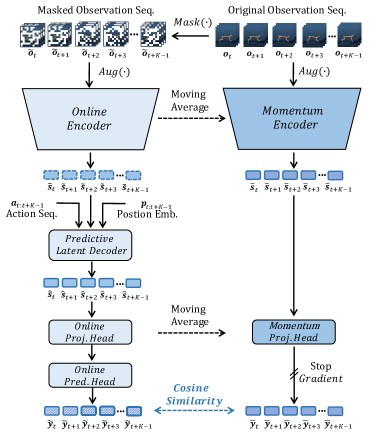
Figure 1: The framework of the proposed MLR. We perform a random spatial-temporal masking (i.e., cube masking) on the sequence of consecutive observations in the pixel space. The masked observations are encoded to be the latent states through an online encoder. We further introduce a predictive latent decoder to decode/predict the latent states conditioned on the corresponding action sequence and temporal positional embeddings. Our method trains the networks to reconstruct the feature representations of the missing contents in an appropriate latent space using a cosine similarity based distance metric applied between the predicted features of the reconstructed states and the target features inferred from original observations by momentum networks.

3 Approach

3.1 Background

Vision-based RL aims to learn policies from pixel observations by interacting with the environment. The learning process corresponds to a partially observable Markov decision process (POMDP) [7, 28], formulated as $(\mathcal{O},\mathcal{A},p,r,\gamma)$, where $\mathcal{O}$, $\mathcal{A}$, $p$, $r$ and $\gamma$ denote the observation space (e.g., pixels), the action space, the transition dynamics $p=Pr(\mathbf{o}_{t+1}|\mathbf{o}_{\leq t},\mathbf{a}_{t})$, the reward function $\mathcal{O}\times\mathcal{A}\to\mathbb{R}$, and the discount factor, respectively. Following common practices [39], an observation $\mathbf{o}_{t}$ is constructed by a few RGB frames. The transition dynamics and the reward function can be formulated as $p_{t}=Pr(\mathbf{o}_{t+1}|\mathbf{o}_{t},\mathbf{a}_{t})$ and $r_{t}=r\left(\mathbf{o}_{t},\mathbf{a}_{t}\right)$, respectively. The objective of RL is to learn a policy $\pi(\mathbf{a}_{t}|\mathbf{o}_{t})$ that maximizes the cumulative discounted return $\mathbb{E}_{\pi}\sum_{t=0}^{\infty}\gamma^{t}r_{t}$, where $\gamma\in[0,1]$.

3.2 Mask-based Latent Reconstruction

Mask-based Latent Reconstruction (MLR) is an auxiliary objective to promote representation learning in vision-based RL and is generally applicable for different RL algorithms, e.g., Soft Actor-Critic (SAC) and Rainbow [26]. The core idea of MLR is to facilitate state representation learning by reconstructing spatially and temporally masked pixels in the latent space. This mechanism enables better use of context information when learning state representations, further enhancing the understanding of RL agents for visual signals. We illustrate the overall framework of MLR in Figure 1 and elaborate on it below.

Framework. In MLR, as shown in Figure 1, we mask a portion of pixels in the input observation sequence along its spatial and temporal dimensions. We encode the masked sequence and the original sequence from observations to latent states with an encoder and a momentum encoder, respectively. We perform predictive reconstruction from the states corresponding to the masked sequence while taking the states encoded from the original sequence as the target. We add reconstruction supervisions between the prediction results and the targets in the decoded latent space. The processes of masking, encoding, decoding and reconstruction are introduced in detail below.

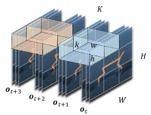
Figure 2: Illustration of our cube masking. We divide the input observation sequence to non-overlapping cubes ($k\times h\times w$). In this example, we have $k=\frac{1}{2}K$, $h=\frac{1}{3}H$ and $w=\frac{1}{3}W$ where the observation sequence has $K=4$ timesteps and a spatial size of $H\times W$.

(i) Masking. Given an observation sequence of $K$ timesteps $\tau_{K}^{o}=\{\textbf{o}_{t},\textbf{o}_{t+1},\cdots,\textbf{o}_{t+K-1}\}$ and each observation containing $n$ RGB frames, all the observations in the sequence are stacked to be a cuboid with the shape of $K\times H\times W$ where $H\times W$ is the spatial size. Note that the actual shape is $K\times H\times W\times D$ where $D=3n$ is the number of channels in each observation. We omit the channel dimension for simplicity. As illustrated in Figure 2, we divide the cuboid into regular non-overlapping cubes with the shape of $k\times h\times w$. We then randomly mask a portion of the cubes following a uniform distribution and obtain a masked observation sequence $\tilde{\tau}_{K}^{o}=\{\tilde{\textbf{o}}_{t},\tilde{\textbf{o}}_{t+1},\cdots,\tilde{\textbf{o}}_{t+K-1}\}$. Following [63], we perform stochastic image augmentation $Aug(\cdot)$ (e.g., random crop and intensity) on each masked observation in $\tilde{\tau}_{K}^{o}$. The objective of MLR is to predict the state representations of the unmasked observation sequence from the masked one in the latent space.

(ii) Encoding. We adopt two encoders to learn state representations from masked observations and original observations respectively. A CNN-based encoder $f$ is used to encode each masked observation $\tilde{\textbf{o}}_{t+i}$ into its corresponding latent state $\mathbf{\tilde{s}}_{t+i}\in\boldsymbol{\mathbb{R}}^{d}$. After the encoding, we obtain a sequence of the masked latent states $\tilde{\tau}_{K}^{s}=\{\mathbf{\tilde{s}}_{t},\mathbf{\tilde{s}}_{t+1},\cdots,\mathbf{\tilde{s}}_{t+K-1}\}$ for masked observations. The parameters of this encoder are updated based on gradient back-propagation in an end-to-end way. We thus call it “online” encoder. The state representations inferred from original observations are taken as the targets of subsequently described reconstruction. To make them more robust, inspired by [32, 46, 63], we exploit another encoder for the encoding of original observations. This encoder, called “momentum” encoder as in Figure 1, has the same architecture as the online encoder, and its parameters are updated by an exponential moving average (EMA) of the online encoder weights $\theta_{f}$ with the momentum coefficient $m\in[0,1)$, as formulated below:

$$\bar{\theta}_{f}\leftarrow m\bar{\theta}_{f}+(1-m)\theta_{f}.$$ (1)

(iii) Decoding. Similar to the mask-based modeling in the CV field, e.g., [25, 58], the online encoder in our MLR predicts the information of the masked contents from the unmasked contents. As opposed to pixel-space reconstruction in [25, 58], MLR performs the reconstruction in the latent space to better perform RL policy learning. Moreover, pixels usually have high information densities [25] which may contain distractions and redundancies for the policy learning in RL. Considering the fact that in RL the next state is determined by the current state as well as the action, we propose to utilize both the actions and states as the inputs for prediction to reduce the possible ambiguity to enable an RL-tailored mask-based modeling design. To this end, we adopt a transformer-based latent decoder to infer the reconstruction results via a global message passing where the actions and temporal information are exploited. Through this process, the predicted information is “passed” to its corresponding state representations.

Figure 3: Illustration of predictive latent decoder.

As shown in Figure 3, the input tokens of the latent decoder consist of both the masked state sequence $\tilde{\tau}_{K}^{s}$ (i.e., state tokens) and the corresponding action sequence $\tau_{K}^{a}=\{\mathbf{a}_{t},\mathbf{a}_{t+1},\cdots,\mathbf{a}_{t+K-1}\}$ (i.e., action tokens). Each action token is embedded as a feature vector with the same dimension as the stated token using an embedding layer, through an embedding layer $Emb(\cdot)$. Following the common practices in transformer-based models [55], we adopt the relative positional embeddings to encode relative temporal positional information into both state and action tokens with an element-wise addition denoted by "$+$" in the following equation (see Appendix B.1 for more details). Notably, the state and action token at the same timestep $t+i$ share the same positional embedding $\mathbf{p}_{t+i}\in\boldsymbol{\mathbb{R}}^{d}$. Thus, the inputs of latent decoder can be mathematically represented as follows:

$$\mathbf{x}=[\mathbf{\tilde{s}}_{t},\mathbf{a}_{t},\mathbf{\tilde{s}}_{t+1},\mathbf{a}_{t+1},\cdots,\mathbf{\tilde{s}}_{t+K-1},\mathbf{a}_{t+K-1}]+[\mathbf{p}_{t},\mathbf{p}_{t},\mathbf{p}_{t+1},\mathbf{p}_{t+1},\cdots,\mathbf{p}_{t+K-1},\mathbf{p}_{t+K-1}].$$ (2)

The input token sequence is fed into a Transformer encoder [55] consisting of $L$ attention layers. Each layer is composed of a Multi-Headed Self-Attention (MSA) layer [55], a layer normalisation (LN) [3], and multilayer perceptron (MLP) blocks. The process can be described as follows:

$$\mathbf{z}^{l}=\boldsymbol{\textrm{MSA}}(\boldsymbol{\textrm{LN}}(\mathbf{x}^{l}))+\mathbf{x}^{l},$$ (3)

$$\mathbf{x}^{l+1}=\boldsymbol{\textrm{MLP}}(\boldsymbol{\textrm{LN}}(\mathbf{z}^{l}))+\mathbf{z}^{l}.$$ (4)

The output tokens of the latent decoder, i.e., $\hat{\tau}_{K}^{s}=\{\mathbf{\hat{s}}_{t},\mathbf{\hat{s}}_{t+1},\cdots,\mathbf{\hat{s}}_{t+K-1}\}$, are the predictive reconstruction results for the latent representations inferred from the original observations. We elaborate on the reconstruction loss between the prediction results and the corresponding targets in the following.

(iv) Reconstruction. Motivated by the success of BYOL [15] in self-supervised learning, we use an asymmetric architecture for calculating the distance between the predicted/reconstructed latent states and the target states, similar to [46, 63]. For the outputs of the latent decoder, we use a projection head $g$ and a prediction head $q$ to get the final prediction result $\mathbf{\hat{y}}_{t+i}=q(g(\mathbf{\hat{s}}_{t+i}))$ corresponding to $\mathbf{s}_{t+i}$. For the encoded results of original observations, we use a momentum-updated projection head $\bar{g}$ whose weights are updated with an EMA of the weights of the online projection head. These two projection heads have the same architectures. The outputs of the momentum projection head $\bar{g}$, i.e., $\mathbf{\bar{y}}_{t+i}=\bar{g}(\mathbf{\bar{s}}_{t+i})$, are the final reconstruction targets. Here, we apply a stop-gradient operation as illustrated in Figure 1 to avoid model collapse, following [15].

The objective of MLR is to enforce the final prediction result $\mathbf{\hat{y}}_{t+i}$ to be as close as possible to its corresponding target $\mathbf{\bar{y}}_{t+i}$. To achieve this, we design the reconstruction loss in our proposed MLR by calculating the cosine similarity between $\mathbf{\hat{y}}_{t+i}$ and $\mathbf{\bar{y}}_{t+i}$, which can be formulated below:

$$\mathcal{L}_{mlr}=1-\frac{1}{K}\sum_{i=0}^{K-1}{\frac{\mathbf{\hat{y}}_{t+i}}{{\left\|\mathbf{\hat{y}}_{t+i}\right\|}_{2}}\frac{\mathbf{\bar{y}}_{t+i}}{{\left\|\mathbf{\bar{y}}_{t+i}\right\|}_{2}}}.$$ (5)

The loss $\mathcal{L}_{mlr}$ is used to update the parameters of the online networks, including encoder $f$, predictive latent decoder $\phi$, projection head $g$ and prediction head $q$. Through our proposed self-supervised auxiliary objective MLR, the learned state representations by the encoder will be more informative and thus can further facilitate policy learning.

Objective. The proposed MLR serves as an auxiliary task, which is optimized together with the policy learning. Thus, the overall loss function $\mathcal{L}_{total}$ for RL agent training is:

$$\mathcal{L}_{total}=\mathcal{L}_{rl}+\lambda\mathcal{L}_{mlr},$$ (6)

where $\mathcal{L}_{rl}$ and $\mathcal{L}_{mlr}$ are the loss functions of the base RL agent (e.g., SAC [18] and Rainbow [26]) and the proposed mask-based latent reconstruction, respectively. $\lambda$ is a hyperparameter for balancing the two terms. Notably, the agent of vision-based RL commonly consists of two parts, i.e., the (state) representation network (i.e., encoder) and the policy learning network. The encoder of MLR is taken as the representation network to encode observations into the state representations for RL training. The latent decoder can be discarded during testing since it is only needed for the optimization with our proposed auxiliary objective during training. More details can be found in Appendix B.

4 Experiment

4.1 Setup

Environments and Evaluation. We evaluate the sample efficiency of our MLR on both the continuous control benchmark DeepMind Control Suite (DMControl) [52] and the discrete control benchmark Atari [5]. On DMControl, following the previous works [32, 60, 31, 63], we choose six commonly used environments from DMControl, i.e., Finger, spin; Cartpole, swingup; Reacher, easy; Cheetah, run; Walker, walk and Ball in cup, catch for the evaluation. We test the performance of RL agents with the mean and median scores over 10 episodes at 100k and 500k environment steps, referred to as DMControl-100k and DMControl-500k benchmarks, respectively. The score of each environment ranges from 0 to 1000 [52]. For discrete control, we test agents on the Atari-100k benchmark [67, 54, 29, 32] which contains 26 Atari games and allows the agents 100k interaction steps (i.e., 400k environment steps with action repeat of 4) for training. Human-normalized score (HNS) is used to measure the performance on each game. Considering the high variance of the scores on this benchmark, we test each run over 100 episodes [46]. To achieve a more rigorous evaluation on high-variance benchmarks such as Atari-100k with a few runs, recent work Rliable [1] systematically studies the evaluation bias issue in deep RL and recommends robust and efficient aggregate metrics to evaluate the overall performance (across all tasks and runs), e.g., interquartile-mean (IQM) and optimality gap (OG) , with percentile confidence intervals (CIs, estimated by the percentile bootstrap with stratified sampling). We follow aforementioned common practices and report the aggregate metrics on the Atari-100k benchmark with 95% CIs.

Implementation. SAC [18] and Rainbow [26] are taken as the base continuous-control agent and discrete-control agent, respectively (see Appendix A.1 and A.2 for the details of the two algorithms). In our experiments, we denote the base agents trained only by RL loss $\mathcal{L}_{rl}$ (as in Equation 6) as Baseline, while denoting the models of applying our proposed MLR to the base agents as MLR for the brevity. Note that compared to naive SAC or Rainbow, our Baseline additionally adopts data augmentation (random crop and random intensity). We adopt this following the prior works [31, 60] which uncovers that applying proper data augmentation can significantly improve the sample efficiency of SAC or Rainbow. As shown in Equation 6, we set a weight $\lambda$ to balance $\mathcal{L}_{rl}$ and $\mathcal{L}_{mlr}$ so that the gradients of these two loss items lie in a similar range and empirically find $\lambda=1$ works well in most environments. In MLR, by default, we set the length of a sampled trajectory $K$ to 16 and mask ratio $\eta$ to 50%. We set the size of the masked cube ($k\times h\times w$) to $8\times 10\times 10$ on most DMControl tasks and $8\times 12\times 12$ on the Atari games. More implementation details can be found in Appendix B.

Table 1: Comparison results (mean $\pm$ std) on the DMControl-100k and DMControl-500k benchmarks. Our method augments Baseline with the proposed MLR objective (denoted as MLR).

100k Step Scores	PlaNet	Dreamer	SAC+AE	SLAC	CURL	DrQ	PlayVirtual	Baseline	MLR
Finger, spin	136 $\pm$ 216	341 $\pm$ 70	740 $\pm$ 64	693 $\pm$ 141	767 $\pm$ 56	901 $\pm$ 104	915 $\pm$ 49	853 $\pm$ 112	907 $\pm$ 58
Cartpole, swingup	297 $\pm$ 39	326 $\pm$ 27	311 $\pm$ 11	-	582 $\pm$ 146	759 $\pm$ 92	816 $\pm$ 36	784 $\pm$ 63	806 $\pm$ 48
Reacher, easy	20 $\pm$ 50	314 $\pm$ 155	274 $\pm$ 14	-	538 $\pm$ 233	601 $\pm$ 213	785 $\pm$ 142	593 $\pm$ 118	866 $\pm$ 103
Cheetah, run	138 $\pm$ 88	235 $\pm$ 137	267 $\pm$ 24	319 $\pm$ 56	299 $\pm$ 48	344 $\pm$ 67	474 $\pm$ 50	399 $\pm$ 80	482 $\pm$ 38
Walker, walk	224 $\pm$ 48	277 $\pm$ 12	394 $\pm$ 22	361 $\pm$ 73	403 $\pm$ 24	612 $\pm$ 164	460 $\pm$ 173	424 $\pm$ 281	643 $\pm$ 114
Ball in cup, catch	0 $\pm$ 0	246 $\pm$ 174	391 $\pm$ 82	512 $\pm$ 110	769 $\pm$ 43	913 $\pm$ 53	926 $\pm$ 31	648 $\pm$ 287	933 $\pm$ 16
Mean	135.8	289.8	396.2	471.3	559.7	688.3	729.3	616.8	772.8
Median	137.0	295.5	351.0	436.5	560.0	685.5	800.5	620.5	836.0
500k Step Scores
Finger, spin	561 $\pm$ 284	796 $\pm$ 183	884 $\pm$ 128	673 $\pm$ 92	926 $\pm$ 45	938 $\pm$ 103	963 $\pm$ 40	944 $\pm$ 97	973 $\pm$ 31
Cartpole, swingup	475 $\pm$ 71	762 $\pm$ 27	735 $\pm$ 63	-	841 $\pm$ 45	868 $\pm$ 10	865 $\pm$ 11	871 $\pm$ 4	872 $\pm$ 5
Reacher, easy	210 $\pm$ 390	793 $\pm$ 164	627 $\pm$ 58	-	929 $\pm$ 44	942 $\pm$ 71	942 $\pm$ 66	943 $\pm$ 52	957 $\pm$ 41
Cheetah, run	305 $\pm$ 131	570 $\pm$ 253	550 $\pm$ 34	640 $\pm$ 19	518 $\pm$ 28	660 $\pm$ 96	719 $\pm$ 51	602 $\pm$ 67	674 $\pm$ 37
Walker, walk	351 $\pm$ 58	897 $\pm$ 49	847 $\pm$ 48	842 $\pm$ 51	902 $\pm$ 43	921 $\pm$ 4575	928 $\pm$ 30	818 $\pm$ 263	939 $\pm$ 10
Ball in cup, catch	460 $\pm$ 380	879 $\pm$ 87	794 $\pm$ 58	852 $\pm$ 71	959 $\pm$ 27	963 $\pm$ 9	967 $\pm$ 5	960 $\pm$ 10	964 $\pm$ 14
Mean	393.7	782.8	739.5	751.8	845.8	882.0	897.3	856.3	896.5
Median	405.5	794.5	764.5	757.5	914.0	929.5	935.0	907.0	948.0

4.2 Comparison with State-of-the-Arts

DMControl. We compare our proposed MLR with the state-of-the-art (SOTA) sample-efficient RL methods proposed for continuous control, including PlaNet [19], Dreamer [20], SAC+AE [61], SLAC [33], CURL [32], DrQ [60] and PlayVirtual [63]. The comparison results are shown in Table 1, and all results are averaged over 10 runs with different random seeds. We can observe that: (i) MLR significantly improves Baseline in both DMControl-100k and DMControl-500k, and achieves consistent gains relative to Baseline across all environments. It is worthy to mention that, for the DMControl-100k, our proposed method outperforms Baseline by 25.3% and 34.7% in mean and median scores, respectively. This demonstrates the superiority of MLR in improving the sample efficiency of RL algorithms. (ii) The RL agent equipped with MLR outperforms most state-of-the-art methods on DMControl-100k and DMControl-500k. Specifically, our method surpasses the best previous method (i.e., PlayVirtual) by 43.5 and 35.5 respectively on mean and median scores on DMControl-100k. Our method also delivers the best median score and reaches a comparable mean score with the strongest SOTA method on DMControl-500k.

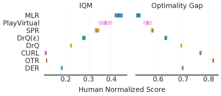
Figure 4: Comparison results on Atari-100k. Aggregate metrics (IQM and optimality gap (OG)) [1] with 95% confidence intervals (CIs) are used for the evaluation. Higher IQM and lower OG are better.

Atari-100k. We further compare MLR with the SOTA model-free methods for discrete control, including DER [54], OTR [29], CURL [32], DrQ [60], DrQ($\epsilon$) (DrQ using the $\epsilon$-greedy parameters in [9]) , SPR [46] and PlayVirtual [63]. These methods and our MLR for Atari are all based on Rainbow [26]. The Atari-100k results are shown in Figure 4. MLR achieves an interquartile-mean (IQM) score of 0.432, which is 28.2% higher than SPR (IQM: 0.337) and 15.5% higher than PlayVirtual (IQM: 0.374). This indicates that MLR has the highest sample efficiency overall. For the optimality gap (OG) metric, MLR reaches an OG of 0.522 which is better than SPR (OG: 0.577) and PlayVirtual (OG: 0.558), showing that our method performs closer to the desired target, i.e., human-level performance. The full scores of MLR (over 3 random seeds) across the 26 Atari games and more comparisons and analysis can be found in Appendix C.1.

4.3 Ablation Study

In this section, we investigate the effectiveness of our MLR auxiliary objective, the impact of masking strategies and the model/method design. Unless otherwise specified, we conduct the ablation studies on the DMControl-100k benchmark and run each model with 5 random seeds.

Effectiveness evaluation. Besides the comparison with SOTA methods, we demonstrate the effectiveness of our proposed MLR by studying its improvements compared to our Baseline. The numerical results are presented in Table 1, while the curves of test performance during the training process are given in Appendix C.2. Both numerical results and test performance curves can demonstrate that our method obviously outperforms Baseline across different environments thanks to more informative representations learned by MLR.

Masking strategy. We compare three design choices of the masking operation: (i) Spatial masking (denoted as MLR-S): we randomly mask patches for each frame independently. (ii) Temporal masking (denoted as MLR-T): we divide the input observation sequence into multiple segments along the temporal dimension and mask out a portion of segments randomly. (Here, the segment length is set to be equal to the temporal length of cube, i.e., $k$.) (iii) Spatial-temporal masking (also referred to as “cube masking”): as aforementioned and illustrated in Figure 2, we rasterize the observation sequence into non-overlapping cubes and randomly mask a portion of them. Except for the differences described above, other configurations for masking remain the same as our proposed spatial-temporal (i.e., cube) masking. From the results in Table 2, we have the following observations: (i) All three masking strategies (i.e., MLR-S, MLR-T and MLR) achieve mean score improvements compared to Baseline by 18.5%, 12.2% and 25.0%, respectively, and achieve median score improvements by 23.4%, 25.0% and 35.9%, respectively. This demonstrates the effectiveness of the core idea of introducing mask-based reconstruction to improve the representation learning of RL. (ii) Spatial-temporal masking is the most effective strategy over these three design choices. This strategy matches better with the nature of video data due to its spatial-temporal continuity in masking. It encourages the state representations to be more predictive and consistent along the spatial and temporal dimensions, thus facilitating policy learning in RL.

Reconstruction target. In masked language/image modeling, reconstruction/prediction is commonly performed in the original signal space, such as word embeddings or pixels. To study the influence of the reconstruction targets for the task of RL, we compare two different reconstruction spaces: (i) Pixel space reconstruction (denoted as MLR-Pixel): we predict the masked contents directly by reconstructing original pixels, like the practices in CV and NLP domains; (ii) Latent space reconstruction (i.e., MLR): we reconstruct the state representations (i.e., features) of original observations from masked observations, as we proposed in MLR. Table 2 shows the comparison results. The reconstruction in the latent space is superior to that in the pixel space in improving sample efficiency. As discussed in the preceding sections, vision data might contain distractions and redundancies for policy learning, making the pixel-level reconstruction unnecessary. Besides, latent space reconstruction is more conducive to the coordination between the representation learning and the policy learning in RL, because the state representations are directly optimized.

Table 2: Ablation study of masking strategy and reconstruction target. We compare three masking strategies: spatial masking (MLR-S), temporal masking (MLR-T) and spatial-temporal masking (MLR), and two reconstruction targets: original pixels (denoted as MLR-Pixel) and momentum projections in the latent space (i.e., MLR).

Environment	Baseline	MLR-S	MLR-T	MLR-Pixel	MLR
Finger, spin	822 $\pm$ 146	919 $\pm$ 55	787 $\pm$ 139	782 $\pm$ 95	907 $\pm$ 69
Cartpole, swingup	782 $\pm$ 74	665 $\pm$ 118	829 $\pm$ 33	803 $\pm$ 91	791 $\pm$ 50
Reacher, easy	557 $\pm$ 137	848 $\pm$ 82	745 $\pm$ 84	787 $\pm$ 136	875 $\pm$ 92
Cheetah, run	438 $\pm$ 33	449 $\pm$ 46	443 $\pm$ 43	346 $\pm$ 84	495 $\pm$ 13
Walker, walk	414 $\pm$ 310	556 $\pm$ 189	393 $\pm$ 202	490 $\pm$ 216	597 $\pm$ 102
Ball in cup, catch	669 $\pm$ 310	927 $\pm$ 6	934 $\pm$ 29	675 $\pm$ 292	939 $\pm$ 9
Mean	613.7	727.3	688.5	647.2	767.3
Median	613.0	756.5	766.0	728.5	833.0

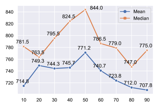
Figure 5: Ablation study of mask ratio.

Mask ratio. In recent works of masked image modeling [25, 58], the mask ratio is found to be crucial for the final performance. We study the influences of different masking ratios on sample efficiency in Figure 5 (with 3 random seeds) and find that the ratio of 50% is an appropriate choice for our proposed MLR. An over-small value of this ratio could not eliminate redundancy, making the objective easy to be reached by extrapolation from neighboring contents that are free of capturing and understanding semantics from visual signals. An over-large value leaves few contexts for achieving the reconstruction goal. As discussed in [25, 58], the choice of this ratio varies for different modalities and depends on the information density of the input signals.

Action token. We study the contributions of action tokens used for the latent decoder in Figure 1 by discarding it from our proposed framework. The results are given in Table 3. Intuitively, prediction only from visual signals is of more or less ambiguity. Exploiting action tokens benefits by reducing such ambiguity so that the gradients of less uncertainty can be obtained for updating the encoder.

Table 3: Ablation studies on action token, masking features and momentum decoder. MLR w.o. ActTok denotes removing the action tokens in the input tokens of the predictive latent decoder. MLR-F indicates performing masking on convolutuional feature maps. MLR-MoDec indicates adding a momentum predictive latent decoder in the target networks.

Environment	Baseline	MLR w.o. ActTok	MLR-F	MLR-MoDec	MLR
Finger, spin	822 $\pm$ 146	832 $\pm$ 46	828 $\pm$ 143	843 $\pm$ 135	907 $\pm$ 69
Cartpole, swingup	782 $\pm$ 74	816 $\pm$ 27	789 $\pm$ 55	766 $\pm$ 88	791 $\pm$ 50
Reacher, easy	557 $\pm$ 137	835 $\pm$ 51	753 $\pm$ 159	800 $\pm$ 49	875 $\pm$ 92
Cheetah, run	438 $\pm$ 33	433 $\pm$ 72	477 $\pm$ 38	470 $\pm$ 12	495 $\pm$ 13
Walker, walk	414 $\pm$ 310	412 $\pm$ 210	673 $\pm$ 33	571 $\pm$ 152	597 $\pm$ 102
Ball in cup, catch	669 $\pm$ 310	837 $\pm$ 114	843 $\pm$ 119	788 $\pm$ 155	939 $\pm$ 9
Mean	613.7	694.2	727.2	706.4	767.3
Median	613.0	824.2	771.0	777.0	833.0

Masking features. We compare “masking pixels” and “masking features” in Table 3. Masking features (denoted by MLR-F) does not perform equally well compared with masking pixels as proposed in MLR, but it still achieves significant improvements relative to Baseline.

Why not use a latent decoder for targets? We have tried to add a momentum-updated latent decoder for obtaining the target states $\mathbf{\bar{s}}_{t+i}$ as illustrated in Figure 1. The results in Table 3 show that adding a momentum decoder leads to performance drops. Since there is no information prediction for the state representation learning from the original observation sequence without masking, we do not need to refine the implicitly predicted information like that in the outputs $\mathbf{\hat{s}}_{t+i}$ of the online encoder.

Table 4: Ablation study of predictive latent decoder depth. We report the number of parameters, mean and median scores on DMControl-100k.

Layers	Param.	Mean	Median
1	20.4K	726.8	719.0
2	40.8K	767.3	833.0
4	81.6K	766.2	789.5
8	163.2K	728.3	763.5

Decoder depth. We analyze the influence of using Transformer-based latent decoders with different depths. We show the experimental results in Table 4. Generally, deeper latent decoders lead to worse sample efficiency with lower mean and median scores. Similar to the designs in [25, 58], it is appropriate to use a lightweight decoder in MLR, because we expect the predicting masked information to be mainly completed by the encoder instead of the decoder. Note that the state representations inferred by the encoder are adopted for the policy learning in RL.

Similarity loss. We compare models using two kinds of similarity metrics to measure the distance in the latent space and observe that using cosine similarity loss is better than using mean squared error (MSE) loss. The results and analysis can be found in Appendix C.2.

Projection and prediction heads. Previous works [15, 46, 11] have shown that in self-supervised learning, supervising the feature representations in the projected space via the projection/prediction heads is often better than in the original feature space. We investigate the effect of the two heads and find that both improve agent performance (see Appendix C.2).

Sequence length and cube size. These two factors can be viewed as hyperparameters. Their corresponding experimental analysis and results are in Appendix C.2.

4.4 More Analysis

We make more detailed investigation and analysis of our MLR from the following aspects with details shown in Appendix C.3. (i) We provide a more detailed analysis of the effect of each masking strategy. (ii) The quality of the learned representations are further evaluated through a pretraining evaluation and a regression accuracy test. (iii) We also investigate the performance of MLR on more challenging control tasks and find that MLR is still effective. (iv) We additionally discuss the relationship between PlayVirtual and MLR. They both achieve leading performance in improving sample efficiency but from different perspectives. (v) We discuss the applications and limitations of MLR. We observe that MLR is more effective on tasks with backgrounds and viewpoints that do not change drastically than on tasks with drastically changing backgrounds/viewpoints or vigorously moving objects.

5 Conclusion

In this work, we make the first effort to introduce the mask-based modeling to RL for facilitating policy learning by improving the learned state representations. We propose MLR, a simple yet effective self-supervised auxiliary objective to reconstruct the masked information in the latent space. In this way, the learned state representations are encouraged to include richer and more informative features. Extensive experiments demonstrate the effectiveness of MLR and show that MLR achieves the state-of-the-art performance on both DeepMind Control and Atari benchmarks. We conduct a detailed ablation study for our proposed designs in MLR and analyze their differences from that in NLP and CV domains. We hope our proposed method can further inspire research for vision-based RL from the perspective of improving representation learning. Moreover, the concept of masked latent reconstruction is also worthy of being explored and extended in CV and NLP fields. We are looking forward to seeing more mutual promotion between different research fields.

Checklist

1. For all authors…

   1. Do the main claims made in the abstract and introduction accurately reflect the paper’s contributions and scope? [Yes]

   2. Did you describe the limitations of your work? [Yes] See Appendix C.3.

   3. Did you discuss any potential negative societal impacts of your work? [Yes] See Appendix D.

   4. Have you read the ethics review guidelines and ensured that your paper conforms to them? [Yes]

2. If you are including theoretical results…

   1. Did you state the full set of assumptions of all theoretical results? [N/A]

   2. Did you include complete proofs of all theoretical results? [N/A]

3. If you ran experiments…

   1. Did you include the code, data, and instructions needed to reproduce the main experimental results (either in the supplemental material or as a URL)? [Yes] https://github.com/microsoft/Mask-based-Latent-Reconstruction.

   2. Did you specify all the training details (e.g., data splits, hyperparameters, how they were chosen)? [Yes] See Appendix B.

   3. Did you report error bars (e.g., with respect to the random seed after running experiments multiple times)? [Yes]

   4. Did you include the total amount of compute and the type of resources used (e.g., type of GPUs, internal cluster, or cloud provider)? [Yes] See Appendix B.

4. If you are using existing assets (e.g., code, data, models) or curating/releasing new assets…

   1. If your work uses existing assets, did you cite the creators? [Yes] See Appendix B.

   2. Did you mention the license of the assets? [Yes] See Appendix B.

   3. Did you include any new assets either in the supplemental material or as a URL? [Yes] https://github.com/microsoft/Mask-based-Latent-Reconstruction.

   4. Did you discuss whether and how consent was obtained from people whose data you’re using/curating? [Yes] See Appendix B.

   5. Did you discuss whether the data you are using/curating contains personally identifiable information or offensive content? [Yes] See Appendix B.

5. If you used crowdsourcing or conducted research with human subjects…

   1. Did you include the full text of instructions given to participants and screenshots, if applicable? [N/A]

   2. Did you describe any potential participant risks, with links to Institutional Review Board (IRB) approvals, if applicable? [N/A]

   3. Did you include the estimated hourly wage paid to participants and the total amount spent on participant compensation? [N/A]

Appendix A Extended Background

A.1 Soft Actor-Critic

Soft Actor-Critic (SAC) [18] is an off-policy actor-critic algorithm, which is based on the maximum entropy RL framework where the standard return maximization objective is augmented with an entropy maximization term [66]. SAC has a soft Q-function $Q$ and a policy $\pi$. The soft Q-function is learned by minimizing the soft Bellman error:

$$\mathit{J}(Q)=\mathbb{E}_{tr\sim\mathcal{D}}[(Q(\mathbf{s}_{t},\mathbf{a}_{t})-(r_{t}+\gamma\bar{V}(\mathbf{s}_{t+1}))^{2}],$$ (7)

where $tr=(\mathbf{s}_{t},\mathbf{a}_{t},r_{t},\mathbf{s}_{t+1})$ is a tuple with current state $\mathbf{s}_{t}$, action $\mathbf{a}_{t}$, successor $\mathbf{s}_{t+1}$ and reward $r_{t}$, $\mathcal{D}$ is the replay buffer and $\bar{\mathit{V}}$ is the target value function. $\bar{\mathit{V}}$ has the following expectation:

$$\bar{V}(\mathbf{s}_{t})=\mathbb{E}_{\mathbf{a}_{t}\sim\pi}[{\bar{Q}{(\mathbf{s}_{t},\mathbf{a}_{t})}-\alpha\log\pi(\mathbf{a}_{t}|\mathbf{s}_{t})}],$$ (8)

where $\bar{Q}$ is the target Q-function whose parameters are updated by an exponential moving average of the parameters of the Q-function $Q$, and the temperature $\alpha$ is used to balance the return maximization and the entropy maximization. The policy $\pi$ is represented by using the reparameterization trick and optimized by minimizing the following objective:

$$J(\pi)=\mathbb{E}_{\mathbf{s}_{t}\sim\mathcal{D},\mathbf{\epsilon}_{t}\sim\mathcal{N}}[\alpha\log\pi(f_{\pi}(\mathbf{\epsilon}_{t};\mathbf{s}_{t})|\mathbf{s}_{t})-Q(\mathbf{s}_{t},f_{\pi}(\mathbf{\epsilon}_{t};\mathbf{s}_{t}))],$$ (9)

where $\mathbf{\epsilon}_{t}$ is the input noise vector sampled from Gaussian distribution $\mathcal{N}(0,I)$, and $f_{\pi}(\mathbf{\epsilon}_{t};\mathbf{s}_{t})$ denotes actions sampled stochastically from the policy $\pi$, i.e., $f_{\pi}(\mathbf{\epsilon}_{t};\mathbf{s}_{t})\sim\tanh(\mu_{\pi}(\mathbf{s}_{t})+\sigma_{\pi}(\mathbf{s}_{t})\odot\mathbf{\epsilon}_{t})$. SAC is shown to have a remarkable performance in continuous control [18].

A.2 Deep Q-network and Rainbow

Deep Q-network (DQN) [39] trains a neural network $\mathit{Q}_{\theta}$ with parameters $\theta$ to approximate the Q-function. DQN introduces a target Q-network $\mathit{Q}_{\theta^{\prime}}$ for stable training. The target Q-network $\mathit{Q}_{\theta^{\prime}}$ has the same architecture as the Q-network $\mathit{Q}_{\theta}$, and the parameters $\theta^{\prime}$ are updated with $\theta$ every certain number of iterations. The objective of DQN is to minimize the squared error between the predictions of $\mathit{Q}_{\theta}$ and the target values provided by $\mathit{Q}_{\theta^{\prime}}$:

$$\mathit{J}(\mathit{Q_{\theta}})=(\mathit{Q}_{\theta}(\mathbf{s}_{t},a_{t})-(r_{t}+\gamma\max\limits_{a}\mathit{Q}_{\theta^{\prime}}(\mathbf{s}_{t+1},a)))^{2}$$ (10)

Rainbow [26] integrates a number of improvements on the basis of the vanilla DQN [39] including: (i) employing modified target Q-value sampling in Double DQN [53]; (ii) adopting Prioritized Experience Replay [44] strategy; (iii) decoupling the value function of state and the advantage function of action from Q-function like Dueling DQN [56]; (iv) introducing distributional RL and predicting value distribution as C51 [6]; (v) adding parametric noise into the network parameters like NoisyNet [14]; and (vi) using multi-step return [50]. Rainbow is typically regarded as a strong model-free baseline for discrete control.

A.3 BYOL-style Auxiliary Objective

BYOL [15] is a strong self-supervised representation learning method by enforcing the similarity of the representations of the same image across diverse data augmentation. The pipeline is shown in Figure 6. BYOL has an online branch and a momentum branch. The momentum branch is used for computing a stable target for learning representations [24, 51]. BYOL is composed of an online encoder $f$, a momentum encoder $\bar{f}$, an online projection head $g$, a momentum projection head $\bar{g}$ and an prediction head $q$. The momentum encoder and projection head have the same architectures as the corresponding online networks and are updated by an exponential moving average (EMA) of the online weights (see Equation 1 in the main manuscript). The prediction head is only used in the online branch, making BYOL’s architecture asymmetric. Given an image $x$, BYOL first produces two views $v$ and $v^{\prime}$ from $x$ through images augmentations. The online branch outputs a representation $y=f(v)$ and a projection $z=g(y)$, and the momentum branch outputs $y^{\prime}=\bar{f}(v^{\prime})$ and a target projection $z^{\prime}=\bar{g}(y^{\prime})$. BYOL then use a prediction head $q$ to regress $z^{\prime}$ from $z$, i.e., $q(z)\rightarrow z^{\prime}$. BYOL minimizes the similarity loss between $q(z)$ and a stop-gradient target $sg(z^{\prime})$.

$$\mathcal{L}_{BYOL}=\left\|q(z)-sg(z^{\prime})\right\|^{2}_{2}=2-2{\frac{q(z)}{{\left\|q(z)\right\|}_{2}}\frac{sg(z^{\prime})}{{\left\|sg(z^{\prime})\right\|}_{2}}}.$$ (11)

Inspired by the success of BYOL in learning visual representations, recent works introduce BYOL-style learning objectives to vision-based RL for learning effective state representations and show promising performance [46, 63, 59, 22, 17]. The BYOL-style learning is often integrated into auxiliary objectives in RL such as future state prediction [46, 17], cycle-consistent dynamics prediction [63], prototypical representation learning [59] and invariant representation learning [22]. These works also show that it is more effective to supervise/regularize the predicted representations in the BYOL’s projected latent space than in the representation or pixel space. Besides, the BYOL-style auxiliary objectives are commonly trained with data augmentation since it can conveniently produce two BYOL views. For example, SPR [46] and PlayVirtual [63] apply random crop and random intensity to input observations in Atari games. The proposed MLR auxiliary objective can be categorized into BYOL-style auxiliary objectives.

Figure 6: An illustration of the framework of BYOL [15].

Appendix B Implementation Detail

B.1 Network Architecture

Our model has two parts: the basic networks and the auxiliary networks. The basic networks are composed of a representation network (i.e., encoder) $f$ parameterized by $\theta_{f}$ and the policy learning networks $\omega$ (e.g., SAC [18] or Rainbow [26]) parameterized by $\theta_{\omega}$.

We follow CURL [32] to build the architecture of the basic networks on the DMControl [52] benchmarks. The encoder is composed of four convolutional layers (with a rectified linear units (ReLU) activation after each), a fully connected (FC) layer, and a layer normalization (LN) [3] layer. Furthermore, the policy learning networks are built by multilayer perceptrons (MLPs). For the basic networks on Atari [5], we also follow CURL to adopt the original architecture of Rainbow [26] where the encoder consists of three convolutional layers (with a ReLU activation after each), and the Q-learning heads are MLPs.

Our auxiliary networks have online networks and momentum (or target) networks. The online networks consist of an encoder $f$, a predictive latent decoder (PLD) $\phi$, a projection head $g$ and a prediction head $q$, parameterized by $\theta_{f}$, $\theta_{\phi}$, $\theta_{g}$ and $\theta_{q}$, respectively. Notably, the encoders in the basic networks and the auxiliary networks are shared. As shown in Figure 1 in our main manuscript, there are a momentum encoder $\bar{f}$ and a momentum projection head $\bar{g}$ for computing the self-supervised targets. The momentum networks have the same architectures as the corresponding online networks. Our PLD is a transformer encoder [55] and has two standard attention layers (with a single attention head). We use an FC layer as the action embedding head to transform the original action into an embedding which has the same dimension as the state representation (i.e., state token). The transformer encoder treats each input token as independent of the other. Thus, positional embeddings, which encode the positional information of tokens in a sequence, are added to the input tokens of PLD to maintain their relative temporal positional information (i.e., the order of the state/action sequences). We use sine and cosine functions to build the positional embeddings following [55]:

$$p_{(pos,2j)}=\sin(pos/10000^{2j/d}),$$ (12)

$$p_{(pos,2j+1)}=\cos(pos/10000^{2j/d}),$$ (13)

where $pos$ is the position, $j$ is the dimension and $d$ is the embedding size (equal to the state representation size). We follow PlayVirtual [63] in the architecture design of the projection and the prediction heads, built by MLPs and FC layers.

B.2 Training Detail

Optimization and training. The training algorithm of our method is presented in Algorithm 1. We use Adam optimizer [30] to optimize all trainable parameters in our model, with $(\beta_{1},\beta_{2})=(0.9,0.999)$ (except for $(0.5,0.999)$ for SAC temperature $\alpha$). Modest data augmentation such as crop/shift is shown to be effective for improving RL agent performance in vision-based RL [60, 31, 46, 63]. Following [63, 46, 32], we use random crop and random intensity in training the auxiliary objective, i.e., $\mathcal{L}_{mlr}$. Besides, we warmup the learning rate of our MLR objective on DMControl by

$$lr=lr_{0}\cdot\min({step\_num}^{-0.5},{step\_num}\cdot{warmup\_step}^{-1.5}),$$ (14)

where the $lr$ and $lr_{0}$ denote the current learning rate and the initial learning rate, respectively, and $step\_num$ and $warmup\_step$ denote the current step and the warmup step, respectively. We empirically find that the warmup schedule bring improvements on DMControl.

Algorithm 1 Training Algorithm for MLR

1:An online encoder $f$, a momentum encoder $\bar{f}$, a predictive latent decoder $\phi$, an online projection head $g$, a momentum projection head $\bar{g}$, a prediction head $q$ and policy learning networks $\omega$, parameterized by $\theta_{f}$, $\bar{\theta}_{f}$, $\theta_{\phi}$, $\theta_{g}$, $\bar{\theta}_{g}$, $\theta_{q}$ and $\theta_{\omega}$, respectively; a stochastic cube masking function $Mask(\cdot)$; a stochastic image augmentation function $Aug(\cdot)$; an optimizer $Optimize(\cdot,\cdot)$.

2:Determine auxiliary loss weight $\lambda$, sequence length $K$, mask ratio $\eta$, cube size $k\times h\times w$ and EMA coefficient $m$.

3:Initialize a replay buffer $\mathcal{D}$.

4:Initialize $Mask(\cdot)$ with $\eta$ and $k\times h\times w$.

5:Initialize all network parameters.

6:while $train$ do

7:     Interact with the environment based on the policy

8:     Collect the transition: $\mathcal{D}\leftarrow\mathcal{D}\cup(\mathbf{o},\mathbf{a},\mathbf{o}_{next},r)$

9:     Sample a trajectory of $K$ timesteps $\{\mathbf{o}_{t},\mathbf{a}_{t},\mathbf{o}_{t+1},\mathbf{a}_{t+1},\cdots,\mathbf{o}_{t+K-1},\mathbf{a}_{t+K-1}\}$ from $\mathcal{D}$

10:     Initialize losses: $\mathcal{L}_{mlr}\leftarrow 0$; $\mathcal{L}_{rl}\leftarrow 0$

11:     Randomly mask the observation sequence:

12:   $\{\mathbf{\tilde{o}}_{t},\mathbf{\tilde{o}}_{t+1},\cdots,\mathbf{\tilde{o}}_{t+K-1}\}\leftarrow Mask(\{\mathbf{o}_{t},\mathbf{o}_{t+1},\cdots,\mathbf{o}_{t+K-1}\})$

13:     Perform augmentation and encoding:

14:   $\{\mathbf{\tilde{s}}_{t},\mathbf{\tilde{s}}_{t+1},\cdots,\mathbf{\tilde{s}}_{t+K-1}\}\leftarrow\{f(Aug(\mathbf{\tilde{o}}_{t})),f(Aug(\mathbf{\tilde{o}}_{t+1})),\cdots,f(Aug({\mathbf{\tilde{o}}_{t+K-1}})\}$

15:     Perform decoding:

16:   $\{\mathbf{\hat{s}}_{t},\mathbf{\hat{s}}_{t+1},\cdots,\mathbf{\hat{s}}_{t+K-1}\}\leftarrow\phi(\{\mathbf{\tilde{s}}_{t},\mathbf{\tilde{s}}_{t+1},\cdots,\mathbf{\tilde{s}}_{t+K-1}\};\{\mathbf{a}_{t},\mathbf{a}_{t+1},\cdots,\mathbf{a}_{t+K-1}\})$

17:     Perform projection and prediction:

18:   $\{\mathbf{\hat{y}}_{t},\mathbf{\hat{y}}_{t+1},\cdots,\mathbf{\hat{y}}_{t+K-1}\}\leftarrow\{q(g(\mathbf{\hat{s}}_{t})),q(g(\mathbf{\hat{s}}_{t+1})),\cdots,q(g(\mathbf{\hat{s}}_{t+K-1}))\}$

19:     Calculate targets:

20:   $\{\mathbf{\bar{y}}_{t},\mathbf{\bar{y}}_{t+1},\cdots,\mathbf{\bar{y}}_{t+K-1}\}\leftarrow\{\bar{g}(\bar{f}(Aug(\mathbf{o}_{t}))),\bar{g}(\bar{f}(Aug(\mathbf{o}_{t+1}))),$

21:                 $\cdots,\bar{g}(\bar{f}(Aug(\mathbf{o}_{t+K-1})))\}$

22:     Calculate MLR loss: $\mathcal{L}_{mlr}\leftarrow 1-\frac{1}{K}\sum_{i=0}^{K-1}{\frac{\mathbf{\hat{y}}_{t+i}}{{\left\|\mathbf{\hat{y}}_{t+i}\right\|}_{2}}\frac{\mathbf{\bar{y}}_{t+i}}{{\left\|\mathbf{\bar{y}}_{t+i}\right\|}_{2}}}$

23:     Calculate RL loss $\mathcal{L}_{rl}$ based on a given base RL algorithm (e.g., SAC)

24:     Calculate total loss: $\mathcal{L}_{total}\leftarrow\mathcal{L}_{rl}+\lambda\mathcal{L}_{mlr}$

25:     Update online parameters: $(\theta_{f},\theta_{\phi},\theta_{g},\theta_{q},\theta_{\omega})\leftarrow Optimize((\theta_{f},\theta_{\phi},\theta_{g},\theta_{q},\theta_{\omega}),\mathcal{L}_{total})$

26:     Update momentum parameters: $(\bar{\theta}_{f},\bar{\theta}_{g})\leftarrow m(\bar{\theta}_{f},\bar{\theta}_{g})+(1-m)(\theta_{f},\theta_{g})$

27:end while

Hyperparameters. We present all hyperparameters used for the DMControl benchmarks [52] in Table 12 and the Atari-100k benchmark in Table 13. We follow prior work [63, 46, 32] for the policy learning hyperparameters (i.e., SAC and Rainbow hyperparameters). The hyperparameters specific to our MLR auxiliary objective, including MLR loss weight $\lambda$, mask ratio $\eta$, the length of the sampled sequence $K$, cube shape $k\times h\times w$ and the depth of the decoder $L$, are shown in the bottom of the tables. By default, we set $\lambda$ to 1, $\eta$ to 50$\%$, $L$ to 2, $k$ to 8, and $h\times w$ to $10\times 10$ on DMControl and $12\times 12$ on Atari. We exceptionally set $k$ to 4 in Cartpole-swingup and Reacher-easy on DMControl due to their large motion range, and $\lambda$ to 5 in Pong and Up N Down on Atari as their MLR losses are relatively smaller than the rest 24 Atari games.

Baseline and data augmentation. Our baseline models (Baseline) are equivalent to CURL [32] without the auxiliary loss except for the slight differences on the applied data augmentation strategies. CURL adopts random crop for data augmentation. We follow the prior work SPR [46] and PlayVirtual [63] to adopt random crop and random intensity for both our Baseline and MLR.

GPU and wall-clock time. In our experiment, we run MLR with a single GPU ( NVIDIA Tesla V100 or GeForce RTX 3090) for each environment. MLR has the same inference time complexity as Baseline since both use only the encoder and policy learning head during testing. On Atari, the average wall-clock training time is 6.0, 10.9, 4.0, and 8.2 hours for SPR, PlayVirtual, Baseline and MLR, respectively. On DMControl, the training time is 4.3, 5.2, 3.8, 6.5 hours for SPR, PlayVirtual, Baseline and MLR, respectively. We will leave the optimization of our training strategy as future work to speed up the training, e.g., reducing the frequency of using masked-latent reconstruction. The evaluation is based on a single GeForce RTX 3090 GPU.

B.3 Environment and Code

DMControl [52] and Atari [5] are widely used environment suites in RL community, which are public and do not involve personally identifiable information or offensive contents. We use the two environment suites to evaluate model performance. The implementation of MLR is based on the open-source PlayVirtual [63] codebase . The statistical tools on Atari are obtained from the open-source library rliable [1].

Appendix C More Experimental Results and Analysis

C.1 More Atari-100k Results

We present the comparison results across all 26 games on the Atari-100k benchmark in Table 5. Our MLR reaches the highest scores on 11 out of 26 games and outperforms the compared methods on the aggregate metrics, i.e., interquartile-mean (IQM) and optimality gap (OG) with 95% confidence intervals (CIs). Notably, MLR improve the Baseline performance by 47.9% on IQM, which shows the effectiveness of our proposed auxiliary objective. We also present the performance profiles using human-normalized scores (HNS) with 95% CIs in Figure 7. The performance profiles confirm the superiority and effectiveness of our MLR. The results of DER [54], OTR [29], CURL [32], DrQ [60] and SPR [46] are from rliable [1], based on 100 random seeds. The results of PlayVirtual [63] are based on 15 random seeds, and the results of Baseline and MLR are averaged over 3 random seeds and each run is evaluated with 100 episodes. We report the standard deviations across runs of Baseline and MLR in Table 6.

Table 5: Comparison on the Atari-100k benchmark. Our method reaches the highest scores on 11 out of 26 games and the best performance concerning the aggregate metrics, i.e., interquartile-mean (IQM) and optimality gap (OG) with 95% confidence intervals. Our method augments Baseline with the MLR objective and achieves a 47.9% relative improvement on IQM.

Game	Human	Random	DER	OTR	CURL	DrQ	SPR	PlayVirtual	Baseline	MLR
Alien	7127.7	227.8	802.3	570.8	711.0	734.1	841.9	947.8	678.5	990.1
Amidar	1719.5	5.8	125.9	77.7	113.7	94.2	179.7	165.3	132.8	227.7
Assault	742.0	222.4	561.5	330.9	500.9	479.5	565.6	702.3	493.3	643.7
Asterix	8503.3	210.0	535.4	334.7	567.2	535.6	962.5	933.3	1021.3	883.7
Bank Heist	753.1	14.2	185.5	55.0	65.3	153.4	345.4	245.9	288.2	180.3
Battle Zone	37187.5	2360.0	8977.0	5139.4	8997.8	10563.6	14834.1	13260.0	13076.7	16080.0
Boxing	12.1	0.1	-0.3	1.6	0.9	6.6	35.7	38.3	14.3	26.4
Breakout	30.5	1.7	9.2	8.1	2.6	15.4	19.6	20.6	16.7	16.8
Chopper Cmd	7387.8	811.0	925.9	813.3	783.5	792.4	946.3	922.4	878.7	910.7
Crazy Climber	35829.4	10780.5	34508.6	14999.3	9154.4	21991.6	36700.5	23176.7	28235.7	24633.3
Demon Attack	1971.0	152.1	627.6	681.6	646.5	1142.4	517.6	1131.7	310.5	854.6
Freeway	29.6	0.0	20.9	11.5	28.3	17.8	19.3	16.1	30.9	30.2
Frostbite	4334.7	65.2	871.0	224.9	1226.5	508.1	1170.7	1984.7	994.3	2381.1
Gopher	2412.5	257.6	467.0	539.4	400.9	618.0	660.6	684.3	650.9	822.3
Hero	30826.4	1027.0	6226.0	5956.5	4987.7	3722.6	5858.6	8597.5	4661.2	7919.3
Jamesbond	302.8	29.0	275.7	88.0	331.0	251.8	366.5	394.7	270.0	423.2
Kangaroo	3035.0	52.0	581.7	348.5	740.2	974.5	3617.4	2384.7	5036.0	8516.0
Krull	2665.5	1598.0	3256.9	3655.9	3049.2	4131.4	3681.6	3880.7	3571.3	3923.1
Kung Fu Master	22736.3	258.5	6580.1	6659.6	8155.6	7154.5	14783.2	14259.0	10517.3	10652.0
Ms Pacman	6951.6	307.3	1187.4	908.0	1064.0	1002.9	1318.4	1335.4	1320.9	1481.3
Pong	14.6	-20.7	-9.7	-2.5	-18.5	-14.3	-5.4	-3.0	-3.1	4.9
Private Eye	69571.3	24.9	72.8	59.6	81.9	24.8	86.0	93.9	93.3	100.0
Qbert	13455.0	163.9	1773.5	552.5	727.0	934.2	866.3	3620.1	553.8	3410.4
Road Runner	7845.0	11.5	11843.4	2606.4	5006.1	8724.7	12213.1	13429.4	12337.0	12049.7
Seaquest	42054.7	68.4	304.6	272.9	315.2	310.5	558.1	532.9	471.9	628.3
Up N Down	11693.2	533.4	3075.0	2331.7	2646.4	3619.1	10859.2	10225.2	4112.8	6675.7
Interquartile Mean	1.000	0.000	0.183	0.117	0.113	0.224	0.337	0.374	0.292	0.432
Optimality Gap	0.000	1.000	0.698	0.819	0.768	0.692	0.577	0.558	0.614	0.522

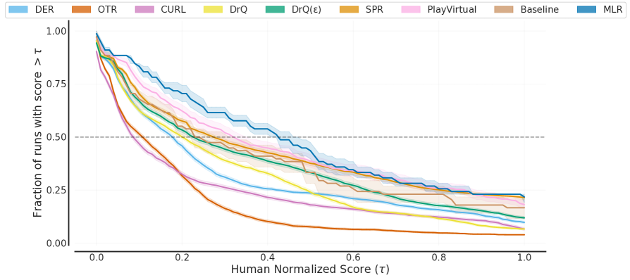
Figure 7: Performance profiles on the Atari-100k benchmark based on human-normalized score distributions. Shaded regions indicates 95% confidence bands. The score distribution of MLR is clearly superior to previous methods and Baseline.

Table 6: Standard deviations (STDs) of Baseline and MLR on Atari-100k. The STDs are calculated based on 3 random seeds.

Game	Baseline	MLR	Game	Baseline	MLR	Game	Baseline	MLR
Alien	61.2	79.2	Crazy Climber	12980.1	2334.5	Kung Fu Master	5026.9	971.8
Amidar	70.7	48.0	Demon Attack	89.8	149.7	Ms Pacman	124.3	249.4
Assault	4.3	28.0	Freeway	0.3	1.0	Pong	11.5	3.1
Asterix	32.1	43.3	Frostbite	1295.3	607.3	Private Eye	11.5	0.0
Bank Heist	39.2	49.7	Gopher	7.9	266.0	Qbert	346.6	96.3
Battle Zone	2070.2	1139.6	Hero	2562.3	692.0	Road Runner	4632.6	669.1
Boxing	7.3	7.4	Jamesbond	108.2	20.8	Seaquest	107.1	92.2
Breakout	1.8	1.4	Kangaroo	3801.2	3025.9	Up N Down	919.3	531.5
Chopper Command	119.9	242.1	Krull	605.9	792.0

C.2 Extended Ablation Study

We give more details of the ablation study. Again, unless otherwise specified, we conduct the ablations on DMControl-100k with 5 random seeds.

Effectiveness evaluation. Besides the numerical results in Table 1 in the main manuscript, we present the test score curves during the training process in Figure 8. Each curve is drawn based on 10 random seeds. The curves demonstrate the effectiveness of the proposed MLR objective. Besides, we observe that MLR achieves more significant gains on the relatively challenging tasks (e.g., Walker-walk and Cheetah-run with six control dimensions) than on the easy tasks (e.g., Cartpole-swingup with a single control dimension). This is because solving challenging tasks often needs more effective representation learning, leaving more room for MLR to play its role.

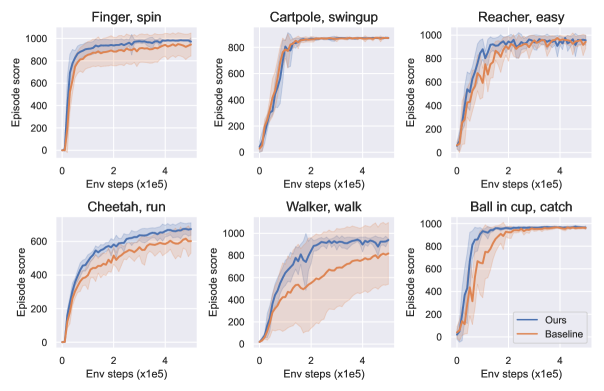
Figure 8: Test performance during the training period (500k environment steps). Lines denote the mean scores over 10 random seeds, and the shadows are the corresponding standard deviations. In most environments on DMControl, our results (blue lines) are consistently better than Baseline (orange lines).

Similarity loss. MLR performs the prediction in the latent space where the value range of the features is unbounded. Using cosine similarity enables the optimization to be conducted in a normalized space, which is more robust to outliers. We compare MLR models using mean squared error (MSE) loss and cosine similarity loss in Table 7. We find that using MSE loss is worse than using cosine similarity loss. Similar observations are found in SPR [46] and BYOL [15].

Projection and prediction heads. MLR adopt the projection and prediction heads following the widely used design in prior works [15, 46]. We study the impact of the heads in Table 7. The results show that using both projection and prediction heads performs best, which is consistent with the observations in the aforementioned prior works.

Table 7: Ablation study of similarity loss (SimLoss), projection (Proj.) and prediction (Pred.) heads.

Model	SimLoss	Proj.	Pred.	Mean	Median
Baseline	-	-	-	613.7	613.0
MLR	Cosine			722.5	770.0
	Cosine		✓	750.3	819.5
	Cosine	✓	✓	767.3	833.0
	MSE	✓	✓	704.8	721.0

Sequence length. Table 8 shows the results of the observation sequence length $K$ at {8, 16, 24}. A large $K$ (e.g., 24) does not bring further performance improvement as the network can reconstruct the missing content in a trivial way like copying and pasting the missing content from other states. In contrast, a small $K$ like 8 may not be sufficient for learning rich context information. A sequence length of 16 is a good trade-off in our experiment.

Table 8: Ablation study of sequence length $K$.

Env.	Baseline	K=8	K=16	K=24
Finger, spin	822 $\pm$ 146	816 $\pm$ 129	907 $\pm$ 69	875 $\pm$ 63
Cartpole, swingup	782 $\pm$ 74	857 $\pm$ 3	791 $\pm$ 50	781 $\pm$ 58
Reacher, easy	557 $\pm$ 137	779 $\pm$ 116	875 $\pm$ 92	736 $\pm$ 247
Cheetah, run	438 $\pm$ 33	469 $\pm$ 51	495 $\pm$ 13	454 $\pm$ 41
Walker, walk	414 $\pm$ 310	473 $\pm$ 264	597 $\pm$ 102	533 $\pm$ 98
Ball in cup, catch	669 $\pm$ 310	910 $\pm$ 58	939 $\pm$ 9	944 $\pm$ 22
Mean	613.7	717.3	767.3	720.5
Median	613.0	797.5	833.0	758.5

Cube size. Our space-time cube can be flexibly designed. We investigate the influence of temporal depth $k$ and the spatial size ($h$ and $w$, $h=w$ by default). The results based on 3 random seeds are shown in Figure 9. In general, a proper cube size leads to good results. The spatial size has a large influence on the final performance. A moderate spatial size (e.g., $10\times 10$) is good for MLR . The performance generally has an upward tendency when increasing the cube depth $k$. However, a cube mask with too large $k$ possibly masks some necessary contents for the reconstruction and hinders the training.

(a) Cube depth $k$

(b) Cube spatial size $h$ & $w$

Figure 9: Ablation studies of (a) cube depth $k$ and (b) cube spatial size $h$ & $w$. The result of each model is averaged over 3 random seeds.

C.3 Discussion

More analysis on MLR-S, MLR-T and MLR. MLR-S masks spatial patches for each frame independently while MLR-T performs masking of entire frames. MLR-S and MLR-T enable a model to capture rich spatial and temporal contexts, respectively. We find that some tasks (e.g., Finger-spin and Walker-walk) have more complicated spatial contents than other tasks on the DMControl benchmarks, requiring stronger spatial modeling capacity. Therefore, MLR-S performs better than MLR-T on these tasks. While for tasks like Cartpole-swingup and Ball-in-cup-catch, where objects have large motion dynamics, temporal contexts are more important, and MLR-T performs better. MLR using space-time masking harnesses both advantages in most cases. But it is slightly inferior to MLR-S/-T in Finger-spin and Cartpole-swingup respectively, due to the sacrifice of full use of spatial or temporal context as in MLR-S or MLR-T.

Evaluation on learned representations. We evaluate the learned representations from two aspects: (i) Pretraining evaluation. We conduct pretraining experiments to test the effectiveness of the learned representation. Data collection: We use a 100k-steps pretrained Baseline model to collect 100k transitions. MLR pretraining: We use the collected data to pretrain MLR without policy learning (i.e., only with MLR objective). Representation testing: We compare two models on DMControl-100k, Baseline with the encoder initialized by the MLR-pretrained encoder (denoted as MLR-Pretraining) and Baseline without pretraining (i.e., Baseline). The results in Table 9 show that MLR-Pretraining outperforms Baseline which is without pretraining but still underperforms MLR which jointly learns the RL objective and the MLR auxiliary objective (also denoted as MLR-Auxiliary). This validates the importance of the learned state representations more directly, but is not the best practice to take the natural of RL into account for getting the most out of MLR. This is because that RL agents learn from interactions with environments, where the experienced states vary as the policy network is updated. (ii) Regression accuracy test. We compute the cosine similarities between the learned representations from the masked observations and those from the corresponding original observations (i.e., observations without masking). The results in Table 10 show that there are high cosine similarity scores of the two representations in MLR while low scores in Baseline. This indicates that the learned representations of MLR are more predictive and informative.

Table 9: Comparison of non-pretraining Baseline (i.e., Baseline), MLR-pretrained Baseline (denoted as MLR-Pretraining) and our joint learning MLR (denoted as MLR-Auxiliary) on DMControl-100k.

DMControl-100k	Cheetah, run	Reacher, easy
Baseline	438 $\pm$ 33	557 $\pm$ 137
MLR-Pretraining	468 $\pm$ 27	862 $\pm$ 180
MLR-Auxiliary	495 $\pm$ 13	875 $\pm$ 92

Table 10: Cosine similarities of the learned representations from the masked observations and those from the original observations in Baseline and MLR.

Cosine Similarity	Cheetah, run	Reacher, easy
Baseline	0.366	0.254
MLR	0.930	0.868

Performance on more challenging control tasks. We further investigate the effectiveness of MLR on more challenging control tasks such as Reacher-hard and Walker-run. We show the test scores based on 3 random seeds at 100k and 500k steps in Table 11. Our MLR still significantly outperforms Baseline.

Table 11: Comparison of Baseline and MLR on more challenging DMControl tasks.

Steps	Model	Reacher, hard	Walker, run
100k	Baseline	341 $\pm$ 275	105 $\pm$ 47
	MLR	624 $\pm$ 220	181 $\pm$ 19
500k	Baseline	669 $\pm$ 290	466 $\pm$ 39
	MLR	844 $\pm$ 129	576 $\pm$ 25

The relationship between PlayVirtual and our MLR. The two works have a consistent purpose, i.e., improving RL sample efficiency, but address this from two different perspectives. PlayVirtual focuses on how to generate more trajectories for enhancing representation learning. In contrast, our MLR focuses on how to exploit the data more efficiently by promoting the model to be predictive of the spatial and temporal context through masking for learning good representations. They are compatible and have their own specialities, while our MLR outperforms PlayVirtual on average.

Application and limitation. While we adopt the proposed MLR objective to two strong baseline algorithms (i.e., SAC and Rainbow) in this work, MLR is a general approach for improving sample efficiency in vision-based RL and can be applied to most existing vision-based RL algorithms (e.g., EfficientZero [62]). We leave more applications of MLR in future work. We have shown the effectiveness of the proposed MLR on multiple continuous and discrete benchmarks. Nevertheless, there are still some limitations to MLR. When we take a closer look at the performance of MLR and Baseline on different kinds of Atari games, we find that MLR brings more significant performance improvement on games with backgrounds and viewpoints that do not change drastically (such as Qbert and Frostbite) than on games with drastically changing backgrounds/viewpoints or vigorously moving objects (such as Crazy Climber and Freeway). This may be because there are low correlations between adjacent regions in spatial and temporal dimensions on the games like Crazy Climber and Freeway so that it is more difficult to exploit the spatial and temporal contexts by our proposed mask-based latent reconstruction. Besides, MLR requires several hyperparameters (such as mask ratio and cube shape) that might need to be adjusted for particular applications.

Appendix D Broader Impact

Although the presented mask-based latent reconstruction (MLR) should be categorized as research in the field of RL, the concept of reconstructing the masked content in the latent space may inspire new approaches and investigations in not only the RL domain but also the fields of computer vision and natural language processing. MLR is simple yet effective and can be conveniently applied to real-world applications such as robotics and gaming AI. However, specific uses may have positive or negative effects (i.e., the dual-use problem). We should follow the responsible AI policies and consider safety and ethical issues in the deployments.

Table 12: Hyperparameters used for DMControl.

Hyperparameter					Value
Frame stack					3
Observation rendering					(100, 100)
Observation downsampling					(84, 84)
Augmentation					Random crop and random intensity
Replay buffer size					100000
Initial exploration steps					1000
Action repeat					2 Finger-spin and Walker-walk;
					8 Cartpole-swingup;
					4 otherwise
Evaluation episodes					10
Optimizer					Adam
$(\beta_{1},\beta_{2})\rightarrow(\theta_{f},\theta_{\phi},\theta_{g},\theta_{q},\theta_{\omega})$					(0.9, 0.999)
$(\beta_{1},\beta_{2})\rightarrow(\alpha)$ (temperature in SAC)					(0.5, 0.999)
Learning rate $(\theta_{f},\theta_{\omega})$					0.0002 Cheetah-run
					0.001 otherwise
Learning rate $(\theta_{f},\theta_{\phi},\theta_{g},\theta_{q})$					0.0001 Cheetah-run
					0.0005 otherwise
Learning rate warmup $(\theta_{f},\theta_{\phi},\theta_{g},\theta_{q})$					6000 steps
Learning rate $(\alpha)$					0.0001
Batch size for policy learning					512
Batch size for auxiliary task					128
Q-function EMA $m$					0.99
Critic target update freq					2
Discount factor					0.99
Initial temperature					0.1
Target network update period					1
Target network EMA $m$					0.9 Walker-walk
					0.95 otherwise
State representation dimension $d$					50
MLR Specific Hyperparameters
Weight of MLR loss $\lambda$					1
Mask ratio $\eta$					50%
Sequence length $K$					16
Cube spatial size $h\times w$					10 $\times$ 10
Cube depth $k$					4 Cartpole-swingup and Reacher-easy
					8 otherwise
Decoder depth $L$ (number of attention layers)					2

Table 13: Hyperparameters used for Atari.

Hyperparameter					Value
Gray-scaling					True
Frame stack					4
Observation downsampling					(84, 84)
Augmentation					Random crop and random intensity
Action repeat					4
Training steps					100K
Max frames per episode					108K
Reply buffer size					100K
Minimum replay size for sampling					2000
Mini-batch size					32
Optimizer					Adam
Optimizer: learning rate					0.0001
Optimizer: $\beta_{1}$					0.9
Optimizer: $\beta_{2}$					0.999
Optimizer: $\epsilon$					0.00015
Max gradient norm					10
Update					Distributional Q
Dueling					True
Support of Q-distribution					51 bins
Discount factor					0.99
Reward clipping Frame stack					[-1, 1]
Priority exponent					0.5
Priority correction					0.4 $\rightarrow$ 1
Exploration					Noisy nets
Noisy nets parameter					0.5
Evaluation trajectories					100
Replay period every					1 step
Updates per step					2
Multi-step return length					10
Q network: channels					32, 64, 64
Q network: filter size					8 $\times$ 8, 4 $\times$ 4, 3 $\times$ 3
Q network: stride					4, 2, 1
Q network: hidden units					256
Target network update period					1
$\tau$ (EMA coefficient)					0
MLR Specific Hyperparameters
Weight of MLR loss $\lambda$					5 Pong and Up N Down
					1 otherwise
Mask ratio $\eta$					50%
Sequence length $K$					16
Cube spatial size $h\times w$					12 $\times$ 12
Cube depth $k$					8
Decoder depth $L$ (number of attention layers)					2

References

- Agarwal et al. [2021] Agarwal, R., Schwarzer, M., Castro, P. S., Courville, A. C., and Bellemare, M. Deep reinforcement learning at the edge of the statistical precipice. Advances in Neural Information Processing Systems, 34, 2021.
- Anand et al. [2019] Anand, A., Racah, E., Ozair, S., Bengio, Y., Côté, M.-A., and Hjelm, R. D. Unsupervised state representation learning in atari. In Advances in Neural Information Processing Systems, 2019.
- Ba et al. [2016] Ba, J. L., Kiros, J. R., and Hinton, G. E. Layer normalization. arXiv preprint arXiv:1607.06450, 2016.
- Bao et al. [2021] Bao, H., Dong, L., Piao, S., and Wei, F. Beit: Bert pre-training of image transformers. In International Conference on Learning Representations, 2021.
- Bellemare et al. [2013] Bellemare, M. G., Naddaf, Y., Veness, J., and Bowling, M. The arcade learning environment: An evaluation platform for general agents. Journal of Artificial Intelligence Research, 47:253–279, 2013.
- Bellemare et al. [2017] Bellemare, M. G., Dabney, W., and Munos, R. A distributional perspective on reinforcement learning. In International Conference on Machine Learning, pp. 449–458. PMLR, 2017.
- Bellman [1957] Bellman, R. A markovian decision process. Journal of mathematics and mechanics, 6(5):679–684, 1957.
- Brown et al. [2020] Brown, T. B., Mann, B., Ryder, N., Subbiah, M., Kaplan, J., Dhariwal, P., Neelakantan, A., Shyam, P., Sastry, G., Askell, A., et al. Language models are few-shot learners. arXiv preprint arXiv:2005.14165, 2020.
- Castro et al. [2018] Castro, P. S., Moitra, S., Gelada, C., Kumar, S., and Bellemare, M. G. Dopamine: A research framework for deep reinforcement learning. arXiv preprint arXiv:1812.06110, 2018.
- Chen et al. [2020a] Chen, M., Radford, A., Child, R., Wu, J., Jun, H., Luan, D., and Sutskever, I. Generative pretraining from pixels. In International Conference on Machine Learning, pp. 1691–1703. PMLR, 2020a.
- Chen et al. [2020b] Chen, T., Kornblith, S., Norouzi, M., and Hinton, G. A simple framework for contrastive learning of visual representations. In International Conference on Machine Learning, pp. 1597–1607. PMLR, 2020b.
- Devlin et al. [2018] Devlin, J., Chang, M.-W., Lee, K., and Toutanova, K. Bert: Pre-training of deep bidirectional transformers for language understanding. arXiv preprint arXiv:1810.04805, 2018.
- Dolan & Moré [2002] Dolan, E. D. and Moré, J. J. Benchmarking optimization software with performance profiles. Mathematical programming, 91(2):201–213, 2002.
- Fortunato et al. [2017] Fortunato, M., Azar, M. G., Piot, B., Menick, J., Osband, I., Graves, A., Mnih, V., Munos, R., Hassabis, D., Pietquin, O., et al. Noisy networks for exploration. arXiv preprint arXiv:1706.10295, 2017.
- Grill et al. [2020] Grill, J.-B., Strub, F., Altché, F., Tallec, C., Richemond, P., Buchatskaya, E., Doersch, C., Avila Pires, B., Guo, Z., Gheshlaghi Azar, M., Piot, B., kavukcuoglu, k., Munos, R., and Valko, M. Bootstrap your own latent - a new approach to self-supervised learning. In Advances in Neural Information Processing Systems, 2020.
- Guo et al. [2020] Guo, Z. D., Pires, B. A., Piot, B., Grill, J.-B., Altché, F., Munos, R., and Azar, M. G. Bootstrap latent-predictive representations for multitask reinforcement learning. In International Conference on Machine Learning, pp. 3875–3886. PMLR, 2020.
- Guo et al. [2022] Guo, Z. D., Thakoor, S., Pîslar, M., Pires, B. A., Altché, F., Tallec, C., Saade, A., Calandriello, D., Grill, J.-B., Tang, Y., et al. Byol-explore: Exploration by bootstrapped prediction. arXiv preprint arXiv:2206.08332, 2022.
- Haarnoja et al. [2018] Haarnoja, T., Zhou, A., Hartikainen, K., Tucker, G., Ha, S., Tan, J., Kumar, V., Zhu, H., Gupta, A., Abbeel, P., et al. Soft actor-critic algorithms and applications. arXiv preprint arXiv:1812.05905, 2018.
- Hafner et al. [2019] Hafner, D., Lillicrap, T., Fischer, I., Villegas, R., Ha, D., Lee, H., and Davidson, J. Learning latent dynamics for planning from pixels. In International Conference on Machine Learning, pp. 2555–2565. PMLR, 2019.
- Hafner et al. [2020a] Hafner, D., Lillicrap, T., Ba, J., and Norouzi, M. Dream to control: Learning behaviors by latent imagination. In International Conference on Learning Representations, 2020a.
- Hafner et al. [2020b] Hafner, D., Lillicrap, T., Norouzi, M., and Ba, J. Mastering atari with discrete world models. arXiv preprint arXiv:2010.02193, 2020b.
- Hansen & Wang [2021] Hansen, N. and Wang, X. Generalization in reinforcement learning by soft data augmentation. In 2021 IEEE International Conference on Robotics and Automation (ICRA), pp. 13611–13617. IEEE, 2021.
- Hansen et al. [2019] Hansen, S., Dabney, W., Barreto, A., Van de Wiele, T., Warde-Farley, D., and Mnih, V. Fast task inference with variational intrinsic successor features. arXiv preprint arXiv:1906.05030, 2019.
- He et al. [2020] He, K., Fan, H., Wu, Y., Xie, S., and Girshick, R. Momentum contrast for unsupervised visual representation learning. In Proceedings of the IEEE/CVF Conference on Computer Vision and Pattern Recognition, pp. 9729–9738, 2020.
- He et al. [2022] He, K., Chen, X., Xie, S., Li, Y., Dollár, P., and Girshick, R. Masked autoencoders are scalable vision learners. In Proceedings of the IEEE/CVF Conference on Computer Vision and Pattern Recognition, pp. 16000–16009, 2022.
- Hessel et al. [2018] Hessel, M., Modayil, J., Van Hasselt, H., Schaul, T., Ostrovski, G., Dabney, W., Horgan, D., Piot, B., Azar, M., and Silver, D. Rainbow: Combining improvements in deep reinforcement learning. In Proceedings of the AAAI Conference on Artificial Intelligence, volume 32, 2018.
- Jaderberg et al. [2016] Jaderberg, M., Mnih, V., Czarnecki, W. M., Schaul, T., Leibo, J. Z., Silver, D., and Kavukcuoglu, K. Reinforcement learning with unsupervised auxiliary tasks. arXiv preprint arXiv:1611.05397, 2016.
- Kaelbling et al. [1998] Kaelbling, L. P., Littman, M. L., and Cassandra, A. R. Planning and acting in partially observable stochastic domains. Artificial intelligence, 101(1-2):99–134, 1998.
- Kielak [2020] Kielak, K. Do recent advancements in model-based deep reinforcement learning really improve data efficiency? arXiv preprint arXiv:2003.10181, 2020.
- Kingma & Ba [2014] Kingma, D. P. and Ba, J. Adam: A method for stochastic optimization. arXiv preprint arXiv:1412.6980, 2014.
- Laskin et al. [2020a] Laskin, M., Lee, K., Stooke, A., Pinto, L., Abbeel, P., and Srinivas, A. Reinforcement learning with augmented data. In Advances in Neural Information Processing Systems, 2020a.
- Laskin et al. [2020b] Laskin, M., Srinivas, A., and Abbeel, P. Curl: Contrastive unsupervised representations for reinforcement learning. In International Conference on Machine Learning, pp. 5639–5650. PMLR, 2020b.
- Lee et al. [2020a] Lee, A. X., Nagabandi, A., Abbeel, P., and Levine, S. Stochastic latent actor-critic: Deep reinforcement learning with a latent variable model. In Advances in Neural Information Processing Systems, 2020a.
- Lee et al. [2020b] Lee, K.-H., Fischer, I., Liu, A., Guo, Y., Lee, H., Canny, J., and Guadarrama, S. Predictive information accelerates learning in RL. arXiv preprint arXiv:2007.12401, 2020b.
- Liu et al. [2021] Liu, G., Zhang, C., Zhao, L., Qin, T., Zhu, J., Jian, L., Yu, N., and Liu, T.-Y. Return-based contrastive representation learning for reinforcement learning. In International Conference on Learning Representations, 2021.
- Liu & Abbeel [2021a] Liu, H. and Abbeel, P. Aps: Active pretraining with successor features. In International Conference on Machine Learning, pp. 6736–6747. PMLR, 2021a.
- Liu & Abbeel [2021b] Liu, H. and Abbeel, P. Behavior from the void: Unsupervised active pre-training. Advances in Neural Information Processing Systems, 34:18459–18473, 2021b.
- Mazoure et al. [2020] Mazoure, B., Tachet des Combes, R., DOAN, T. L., Bachman, P., and Hjelm, R. D. Deep reinforcement and infomax learning. In Advances in Neural Information Processing Systems, 2020.
- Mnih et al. [2013] Mnih, V., Kavukcuoglu, K., Silver, D., Graves, A., Antonoglou, I., Wierstra, D., and Riedmiller, M. Playing atari with deep reinforcement learning. arXiv preprint arXiv:1312.5602, 2013.
- Oord et al. [2018] Oord, A. v. d., Li, Y., and Vinyals, O. Representation learning with contrastive predictive coding. arXiv preprint arXiv:1807.03748, 2018.
- Pathak et al. [2016] Pathak, D., Krahenbuhl, P., Donahue, J., Darrell, T., and Efros, A. A. Context encoders: Feature learning by inpainting. In Proceedings of the IEEE conference on computer vision and pattern recognition, pp. 2536–2544, 2016.
- Radford et al. [2018] Radford, A., Narasimhan, K., Salimans, T., and Sutskever, I. Improving language understanding by generative pre-training. 2018.
- Radford et al. [2019] Radford, A., Wu, J., Child, R., Luan, D., Amodei, D., Sutskever, I., et al. Language models are unsupervised multitask learners. OpenAI blog, 1(8):9, 2019.
- Schaul et al. [2015] Schaul, T., Quan, J., Antonoglou, I., and Silver, D. Prioritized experience replay. arXiv preprint arXiv:1511.05952, 2015.
- Schrittwieser et al. [2020] Schrittwieser, J., Antonoglou, I., Hubert, T., Simonyan, K., Sifre, L., Schmitt, S., Guez, A., Lockhart, E., Hassabis, D., Graepel, T., et al. Mastering atari, go, chess and shogi by planning with a learned model. Nature, 588(7839):604–609, 2020.
- Schwarzer et al. [2021a] Schwarzer, M., Anand, A., Goel, R., Hjelm, R. D., Courville, A., and Bachman, P. Data-efficient reinforcement learning with self-predictive representations. In International Conference on Learning Representations, 2021a.
- Schwarzer et al. [2021b] Schwarzer, M., Rajkumar, N., Noukhovitch, M., Anand, A., Charlin, L., Hjelm, R. D., Bachman, P., and Courville, A. C. Pretraining representations for data-efficient reinforcement learning. Advances in Neural Information Processing Systems, 34:12686–12699, 2021b.
- Shelhamer et al. [2017] Shelhamer, E., Mahmoudieh, P., Argus, M., and Darrell, T. Loss is its own reward: Self-supervision for reinforcement learning. ArXiv, abs/1612.07307, 2017.
- Stooke et al. [2020] Stooke, A., Lee, K., Abbeel, P., and Laskin, M. Decoupling representation learning from reinforcement learning. arXiv preprint arXiv:2009.08319, 2020.
- Sutton & Barto [2018] Sutton, R. S. and Barto, A. G. Reinforcement learning: An introduction. MIT press, 2018.
- Tarvainen & Valpola [2017] Tarvainen, A. and Valpola, H. Mean teachers are better role models: Weight-averaged consistency targets improve semi-supervised deep learning results. Advances in neural information processing systems, 30, 2017.
- Tassa et al. [2018] Tassa, Y., Doron, Y., Muldal, A., Erez, T., Li, Y., Casas, D. d. L., Budden, D., Abdolmaleki, A., Merel, J., Lefrancq, A., et al. Deepmind control suite. arXiv preprint arXiv:1801.00690, 2018.
- Van Hasselt et al. [2016] Van Hasselt, H., Guez, A., and Silver, D. Deep reinforcement learning with double q-learning. In Proceedings of the AAAI Conference on Artificial Intelligence, volume 30, 2016.
- van Hasselt et al. [2019] van Hasselt, H. P., Hessel, M., and Aslanides, J. When to use parametric models in reinforcement learning? In Advances in Neural Information Processing Systems, 2019.
- Vaswani et al. [2017] Vaswani, A., Shazeer, N., Parmar, N., Uszkoreit, J., Jones, L., Gomez, A. N., Kaiser, Ł., and Polosukhin, I. Attention is all you need. In Advances in neural information processing systems, pp. 5998–6008, 2017.
- Wang et al. [2016] Wang, Z., Schaul, T., Hessel, M., Hasselt, H., Lanctot, M., and Freitas, N. Dueling network architectures for deep reinforcement learning. In International Conference on Machine Learning, pp. 1995–2003. PMLR, 2016.
- Wei et al. [2022] Wei, C., Fan, H., Xie, S., Wu, C.-Y., Yuille, A., and Feichtenhofer, C. Masked feature prediction for self-supervised visual pre-training. In Proceedings of the IEEE/CVF Conference on Computer Vision and Pattern Recognition, pp. 14668–14678, 2022.
- Xie et al. [2022] Xie, Z., Zhang, Z., Cao, Y., Lin, Y., Bao, J., Yao, Z., Dai, Q., and Hu, H. Simmim: A simple framework for masked image modeling. In Proceedings of the IEEE/CVF Conference on Computer Vision and Pattern Recognition, pp. 9653–9663, 2022.
- Yarats et al. [2021a] Yarats, D., Fergus, R., Lazaric, A., and Pinto, L. Reinforcement learning with prototypical representations. In International Conference on Machine Learning, pp. 11920–11931. PMLR, 2021a.
- Yarats et al. [2021b] Yarats, D., Kostrikov, I., and Fergus, R. Image augmentation is all you need: Regularizing deep reinforcement learning from pixels. In International Conference on Learning Representations, 2021b.
- Yarats et al. [2021c] Yarats, D., Zhang, A., Kostrikov, I., Amos, B., Pineau, J., and Fergus, R. Improving sample efficiency in model-free reinforcement learning from images. In Proceedings of the AAAI Conference on Artificial Intelligence, volume 35, pp. 10674–10681, 2021c.
- Ye et al. [2021] Ye, W., Liu, S., Kurutach, T., Abbeel, P., and Gao, Y. Mastering atari games with limited data. Advances in Neural Information Processing Systems, 34, 2021.
- Yu et al. [2021] Yu, T., Lan, C., Zeng, W., Feng, M., Zhang, Z., and Chen, Z. Playvirtual: Augmenting cycle-consistent virtual trajectories for reinforcement learning. In Advances in Neural Information Processing Systems, 2021.
- Zhang et al. [2021] Zhang, A., McAllister, R. T., Calandra, R., Gal, Y., and Levine, S. Learning invariant representations for reinforcement learning without reconstruction. In International Conference on Learning Representations, 2021.
- Zhu et al. [2020] Zhu, J., Xia, Y., Wu, L., Deng, J., Zhou, W., Qin, T., and Li, H. Masked contrastive representation learning for reinforcement learning. arXiv preprint arXiv:2010.07470, 2020.
- Ziebart et al. [2008] Ziebart, B. D., Maas, A. L., Bagnell, J. A., Dey, A. K., et al. Maximum entropy inverse reinforcement learning. In AAAI, volume 8, pp. 1433–1438. Chicago, IL, USA, 2008.
- Łukasz Kaiser et al. [2020] Łukasz Kaiser, Babaeizadeh, M., Miłos, P., Osiński, B., Campbell, R. H., Czechowski, K., Erhan, D., Finn, C., Kozakowski, P., Levine, S., Mohiuddin, A., Sepassi, R., Tucker, G., and Michalewski, H. Model based reinforcement learning for atari. In International Conference on Learning Representations, 2020.