Linear Adversarial Concept Erasure

Abstract

Modern neural models trained on textual data rely on pre-trained representations that emerge without direct supervision. As the use of these representations in real-world applications increases, our inability to control their content becomes a pressing problem. This paper formulates the problem of identifying and erasing a linear subspace that corresponds to a given concept in order to prevent linear predictors from recovering the concept. Our formulation consists of a constrained, linear minimax game. We consider different concept-identification objectives, modeled after several tasks such as classification and regression. We derive a closed-form solution for certain objectives, and propose a convex relaxation, R-LACE , that works well for others. When evaluated in the context of binary gender removal, our method recovers a low-dimensional subspace whose removal mitigates bias as measured by intrinsic and extrinsic evaluation. We show that the method—despite being linear—is highly expressive, effectively mitigating bias in deep nonlinear classifiers while maintaining tractability and interpretability.

https://github.com/shauli-ravfogel/rlace-icml

1 Introduction

This paper studies concept erasure, the removal of information from a given vector representation, such as those that are derived from neural language models (Melamud et al., 2016; Peters et al., 2018; Howard and Ruder, 2018; Devlin et al., 2019).

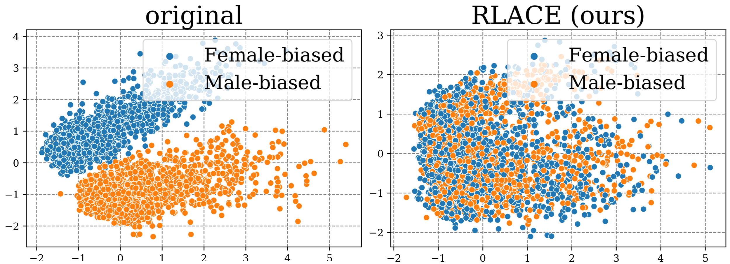
Figure 1: Removal of gender information from GloVe representations using R-LACE , after PCA (Experiment § 5.1). Left: original space; Right: after a rank-1 R-LACE projection. Word vectors are colored according to being male-biased of female-biased.

Specifically, we ask the following question: Given a set of vectors $\boldsymbol{x}_{1},\dots,\boldsymbol{x}_{N}\in\mathbb{R}^{D}$, and corresponding response variables $y_{1},\dots,y_{N}$, can we derive a concept-erasure function $r(\cdot)$ such that the resulting vectors $r(\boldsymbol{x}_{1}),\dots,r(\boldsymbol{x}_{N})$ are not predictive of the concept $y_{1},\dots,y_{N}$, but such that $r(\boldsymbol{x}_{n})$ preserves the information found in $\boldsymbol{x}_{n}$ as much as possible? This problem relates to the more general question of obtaining representations that do not contain information about a given concept, however, unlike adversarial methods (Edwards and Storkey, 2016; Xie et al., 2017; Chen et al., 2018; Elazar and Goldberg, 2018; Zhang et al., 2018) that change the model during training, here we are interested in post-hoc methods, which assume a fixed, pre-trained set of vectors, e.g., those from GloVe (Pennington et al., 2014), BERT (Devlin et al., 2019), or GPT (Radford et al., 2019), and aim to learn an additional function $r(\cdot)$ that removes information from the set of vectors.

In this work, we focus on the case where the function $r(\cdot)$ is linear—in other words, we aim to identify and remove a linear concept subspace from the representation, preventing any linear predictor from recovering the concept. By restricting ourselves to the linear case, we obtain a tractable solution while also enjoying the increased interpretability of linear methods.

Linear concept removal was pioneered by Bolukbasi et al. (2016), who used principal component analysis to identify a linear gender bias subspace. Another linear concept removal technique is iterative nullspace projection (INLP; Ravfogel et al., 2020). INLP learns the linear bias subspace by first training a classifier on a task that operationalizes the concept (e.g., binary gender prediction) and then isolating the concept subspace using the classifier’s learned weights.

We introduce a principled framework for linear concept erasure in the form of a linear minimax game (von Neumann and Morgenstern, 1947). In many cases, we find that this minimax formulation offers superior performance to previously proposed methods, e.g., INLP. Moreover, because the game is linear, we still retain an interpretable concept space. Given this framework, we are able to derive a closed-form solution to the minimax problem in several cases, such as linear regression and Rayleigh quotient maximization. Further, we develop a convex relaxation, Relaxed Linear Adversarial Concept Erasure (R-LACE), that allows us to find a good solution in practice for the case of classification, e.g., logistic regression. In the empirical portion of the paper, we experiment with removing information predictive of binary gender, and find our minimax formulation effective in mitigating bias in both uncontexualized, e.g., GloVe, and contextualized, e.g., BERT, representations.

2 Linear Minimax Games

This section focuses on the mathematical preliminaries necessary to develop linear adversarial concept removal. Specifically, we formulate the problem as a minimax game between a predictor that aims to predict a quantity that operationalizes the concept that tries to hinder the prediction by projecting the input embeddings to a subspace of predefined dimensionality. By constraining the adversarial intervention to a linear projection, we maintain the advantages of linear methods—interpretability and transparency—while directly optimizing an expressive objective that aims to prevent any linear model from predicting the concept of interest.

2.1 Notation and Generalized Linear Modeling

We briefly overview generalized linear modeling (Nelder and Wedderburn, 1972) as a unified framework that encompasses many different linear models. e.g., linear regression and logistic regression.

Notation.

We consider the problem where we are given a dataset ${\mathcal{D}}=\{(y_{n},\boldsymbol{x}_{n})\}_{n=1}^{N}$ of $N$ response–representation pairs, where the response variables $y_{n}$ represent the information to be neutralized (e.g., binary gender).

In this work, we take $y_{n}\in\mathbb{R}$ to be a real value and $\boldsymbol{x}_{n}\in\mathbb{R}^{D}$ to be a $D$-dimensional real column vector. We use the notation $X={[\boldsymbol{x}_{1}^{\top},\dots,\boldsymbol{x}_{N}^{\top}]}^{\top}\in\mathbb{R}^{N\times D}$ to denote a matrix containing the inputs, and $\boldsymbol{y}=[y_{1},\dots,y_{N}]^{\top}\in\mathbb{R}^{N}$ to denote a vector containing all the response variables.

Generalized Linear Models.

We unify several different linear concept-removal objectives in the framework of generalized linear modeling. A linear model is a predictor of the form $\widehat{y}_{n}={\boldsymbol{\theta}}^{\top}\boldsymbol{x}_{n}$, where the model’s parameters ${\boldsymbol{\theta}}$ come from some set $\Theta$. In the case of a generalized linear model, the predictor is coupled with a link function $g(\cdot)$. The link function allows us to relate the linear prediction to the response in a more nuanced (perhaps non-linear) way. We denote the link function’s inverse as $g^{-1}\!\left(\cdot\right)$. Using this notation, the predictor of a generalized linear model is $\widehat{y}_{n}=g^{-1}\!\left({\boldsymbol{\theta}}^{\top}\boldsymbol{x}_{n}\right)$. We additionally assume a loss function $\ell(\cdot,\cdot)\geq 0$, a non-negative function of the true response $y_{n}$ and a predicted response $\widehat{y}_{n}$, which is to be minimized. By changing the link function and the loss function we obtain different problems such as linear regression, Rayleigh quotient problems, SVM, logistic regression classification inter alia. Now, we consider the objective

$$\sum_{n=1}^{N}\ell\left(y_{n},\widehat{y}_{n}\right) =\sum_{n=1}^{N}\ell\left(y_{n},g^{-1}\!\left({\boldsymbol{\theta}}^{\top}\boldsymbol{x}_{n}\right)\right)$$ (1)

We seek to minimize 1 with respect to ${\boldsymbol{\theta}}$ in order to learn a good predictor of $y_{n}$ from $\boldsymbol{x}_{n}$.

2.2 The Linear Bias Subspace Hypothesis

Consider a collection $\{\boldsymbol{x}_{m}\}_{m=1}^{M}$ of $M$ representations where $\boldsymbol{x}_{m}\in\mathbb{R}^{D}$. The linear bias subspace hypothesis (Bolukbasi et al., 2016; Vargas and Cotterell, 2020) posits that there exists a linear subspace $B\subseteq\mathbb{R}^{D}$ that (fully) contains gender bias information within representations $\{\boldsymbol{x}_{m}\}_{m=1}^{M}$. It follows from this hypothesis that one strategy for the removal of gender information from representations is to i) identify the subspace $B$ and ii) to project the representations on to the orthogonal complement of $B$, i.e., re-define every representation $\boldsymbol{x}_{m}$ in our collection as

$$\overline{\boldsymbol{x}}_{m}={{{\footnotesize\textsf{proj}}_{B_{\perp}}}(\boldsymbol{x}_{m})}$$ (2)

Basic linear algebra tells us that the operation ${{\footnotesize\textsf{proj}}_{B_{\perp}}}$ is represented by an orthogonal projection matrix, i.e., there is a symmetric matrix $P$ such that $P^{2}=P$ and ${{\footnotesize\textsf{proj}}_{B_{\perp}}}(\boldsymbol{x}_{m})=P\boldsymbol{x}_{m}$. This means that ${{\footnotesize\textsf{null}}}(P)$ is our bias subspace and ${{\footnotesize\textsf{range}}}(P)$ is its orthogonal complement, i.e., the space without the bias subspace. Intuitively, an orthogonal projection matrix onto a subspace maps a vector to its closest neighbor on the subspace. In our case, the projection maps a vector to the closest vector in the subspace that excludes the bias subspace.

2.3 Linear Minimax Games

We are now in a position to define a linear minimax game that adversarially identifies and removes a linear bias subspace. Following Ravfogel et al. (2020), we search for an orthogonal projection matrix $P$ that projects onto $B_{\perp}$, i.e., the orthogonal complement of the bias subspace $B$. We define $\mathcal{P}_{k}$ as the set of all $D\times D$ orthogonal projection matrices that neutralize a rank $k$ subspace. More formally, we have that

$$P\in\mathcal{P}_{k}\leftrightarrow\underbrace{P=I_{D}-W^{\top}W}_{\text{Projects to }\textsf{null}(W)},\,\underbrace{W\in\mathbb{R}^{k\times D}}_{\mathrm{rank(W)}\leq k},\,\underbrace{WW^{\top}=I_{k}}_{\text{orthogonal}}$$ (3)

where $I_{k}$ denotes the $k\times k$ identity matrix and $I_{D}$ denotes the $D\times D$ identity matrix. The matrix $P$ neutralizes the $k$-dimensional subspace $B=\texttt{span}(W)$.

We define a minimax game between $P\in\mathcal{P}_{k}$ and ${\boldsymbol{\theta}}$:

$$\min_{{\boldsymbol{\theta}}\in\Theta}\,\max_{{P\in\mathcal{P}_{k}}}\,\sum_{n=1}^{N}\ell\Big{(}y_{n},\,g^{-1}\!\left({\boldsymbol{\theta}}^{\top}P\boldsymbol{x}_{n}\right)\Big{)}$$ (4)

where $k$—the dimensionality of the neutralized subspace—is an hyperparamter. Note that 4 is a special case of the general adversarial training algorithm (Goodfellow et al., 2014), but where the adversary is constrained to interact with the input only via an orthogonal projection matrix of rank at most $k$. This constraint enables us to derive principled solutions, while minimally changing the input.

We now spell out several instantiations of common linear models within the framework of adversarial generalized linear modeling: (i) linear regression, (ii) partial least squares regression, and (iii) logistic regression.

Example Linear Regression.

Consider the loss function $\ell(y,\widehat{y})={||y-\widehat{y}||}^{2}$, the parameter space $\Theta=\mathbb{R}^{D}$, and the inverse link function $g^{-1}\!\left(z\right)=z$. Then 4 corresponds to

$$\min_{{\boldsymbol{\theta}}\in\mathbb{R}^{D}}\max_{P\in\mathcal{P}_{k}}\,\,\sum_{n=1}^{N}{||y_{n}-{\boldsymbol{\theta}}^{\top}P\boldsymbol{x}_{n}||}^{2}$$ (5)

Example Partial Least Squares Regression.

Consider the loss function $\ell(y,\widehat{y})={(y\widehat{y})}^{2}$, $g^{-1}\!\left(z\right)=z$, and $\Theta_{P}=\{{\boldsymbol{\theta}}P\mid||{\boldsymbol{\theta}}P||^{2}=1\}$ where the parameter space $\Theta_{P}$ is dependent on $P$. Then 4 corresponds to

$$\min_{{\boldsymbol{\theta}}\in\mathbb{R}^{D}}\max_{\begin{subarray}{c}P\in\mathcal{P}_{k},\\ ||P{\boldsymbol{\theta}}||^{2}=1\end{subarray}}\,\,\sum_{n=1}^{N}||y_{n}{\boldsymbol{\theta}}^{\top}P\boldsymbol{x}_{n}||^{2}$$ (6)

Example Logistic Regression.

Consider the loss function $\ell(y,\widehat{y})=y\log\widehat{y}$, the parameter space $\Theta=\mathbb{R}^{D}$, and the link function $g^{-1}\!\left(z\right)=\frac{\exp z}{1+\exp z}$. Then 4 corresponds to

$$\min_{{\boldsymbol{\theta}}\in\mathbb{R}^{D}}\max_{P\in\mathcal{P}_{k}}\,\,\sum_{n=1}^{N}y_{n}\log\frac{\exp{\boldsymbol{\theta}}^{\top}P\boldsymbol{x}_{n}}{1+\exp{\boldsymbol{\theta}}^{\top}P\boldsymbol{x}_{n}}$$ (7)

3 Solving the Linear Minimax Game

How can we effectively prevent a given generalized linear model from recovering a concept of interest from the representation? At the technical level, the above reduces to a simple question: For which pairs of $\ell(\cdot,\cdot)$ and $g^{-1}\!\left(\cdot\right)$ can we solve the objective given in § 2? We find a series of satisfying answers. In the case of linear regression (Example 1) and Rayleigh quotient problems (such as partial least squares regression, Example 2) we derive a closed-form solution. And, in the case of Example 3, we derive a convex relaxation that can be solved effectively with gradient-based optimization.

3.1 Linear Regression

We begin with the case of linear regression (Example 1). We show that there exists an optimal solution to 5 in the following proposition, proved in § B.3.

Proposition 3.1.

The equilibrium point of the objective below

$$\min_{{\boldsymbol{\theta}}\in\mathbb{R}^{D}}\max_{P\in\mathcal{P}_{k}}\,\,\sum_{n=1}^{N}{||y_{n}-{\boldsymbol{\theta}}^{\top}P\boldsymbol{x}_{n}||}^{2}$$ (8)

$$(=)\min_{{\boldsymbol{\theta}}\in\mathbb{R}^{D}}\max_{P\in\mathcal{P}_{k}}\,\,{||\boldsymbol{y}-XP{\boldsymbol{\theta}}||}^{2}$$ (9)

is achieved when $P=I-\frac{X^{\top}\boldsymbol{y}\boldsymbol{y}X}{\boldsymbol{y}^{\top}XX^{\top}\boldsymbol{y}}$. At this point, the objective is equal to the variance of $\boldsymbol{y}$.

Note that the optimal direction for linear regression, $X^{\top}\boldsymbol{y}$, is the covariance between the input and the target. As the regression target is one dimensional, the covariance is a single vector. Since linear regression aims to explain the covariance, once this single direction is neutralized, the input becomes completely uninformative with respect to $\boldsymbol{y}$.

3.2 Rayleigh Quotient Maximization

We now turn to partial least squares regression (Wold, 1973) as a representative of a special class of objectives, which also include canonical correlation analysis (Hotelling and Pabst, 1936) and other problems. The loss function described in Example 2 is not convex due to the constraint that the parameters have unit norm. However, we can still efficiently minimize the objective making use of basic results in linear algebra. We term losses of the type in 6 Rayleigh quotient losses because they may be formulated as a Rayleigh quotient (Horn and Johnson, 2012).

We now state a general lemma about minimax games in the form of a Rayleigh quotient. This lemma allows us to show that Example 2 can be solved exactly.

Lemma 3.2.

Let $A\in\mathbb{R}^{D\times D}$ be a symmetric matrix. Let $A=V^{\top}\Lambda V$ be the eigendecomposition of $A$. We order the orthonormal eigenbasis $\{\boldsymbol{v}_{1},\ldots,\boldsymbol{v}_{D}\}$ such that the corresponding eigenvalues are ordered: $\lambda_{1}\geq\lambda_{2}\cdots\geq\lambda_{D}$. Then the following saddle point problem

$$\max_{{\boldsymbol{\theta}}\in\mathbb{R}^{D}}\min_{P\in\mathcal{P}_{k}}\frac{{\boldsymbol{\theta}}^{\top}P^{\top}AP{\boldsymbol{\theta}}}{||P{\boldsymbol{\theta}}||_{2}^{2}}$$ (10)

where the constraint enforces that $P$ is an orthogonal projection matrix of rank $k$, has the solution

$${\boldsymbol{\theta}}^{\star} =\boldsymbol{v}_{k+1}$$ (11)

$$P^{\star} =I-\sum_{d=1}^{D-k}\boldsymbol{v}_{d}\boldsymbol{v}_{d}^{\top}$$ (12)

Moreover, the value of 10 is $\lambda_{k+1}$.

This lemma is proved in § B.2.

Proposition 3.3.

The PLS objective 6 has an equilibrium point where ${\boldsymbol{\theta}}$ and $P$ are given by 11 and 12.

Proof.

The adversarial PLS objective Example 2 is scale invariant. Thus, it can be equivalently expressed as

$$\min_{{\boldsymbol{\theta}}\in\mathbb{R}^{D}}\max_{\begin{subarray}{c}P\in\mathcal{P}_{k},\\ ||P{\boldsymbol{\theta}}||^{2}=1\end{subarray}}\,\,\sum_{n=1}^{N}||{\boldsymbol{\theta}}^{\top}P\boldsymbol{x}_{n}y_{n}||^{2}$$ (13)

$$=\min_{{\boldsymbol{\theta}}\in\mathbb{R}^{D}}\max_{\begin{subarray}{c}P\in\mathcal{P}_{k},\\ ||P{\boldsymbol{\theta}}||^{2}=1\end{subarray}}\,\,{\boldsymbol{\theta}}^{\top}PX^{\top}\boldsymbol{y}\boldsymbol{y}^{\top}XP{\boldsymbol{\theta}}$$ (14)

$$=\min_{{\boldsymbol{\theta}}\in\mathbb{R}^{D}}\max_{\begin{subarray}{c}P\in\mathcal{P}_{k}\end{subarray}}\,\,\frac{{\boldsymbol{\theta}}^{\top}PX^{\top}\boldsymbol{y}\boldsymbol{y}^{\top}XP{\boldsymbol{\theta}}}{||P{\boldsymbol{\theta}}||}$$ (15)

The above is in the form 10 if we take $A=X^{\top}\boldsymbol{y}\boldsymbol{y}^{\top}X$. ∎

3.3 Classification

We now turn to the case of logistic regression. In this case, we are not able to identify a closed-form solution, so we propose a practical convex relaxation of the problem that can be solved with iterative methods. Note that while our exposition focuses on logistic regression, any other convex loss, e.g., hinge loss, may be substituted in.

Convex–Concave Games.

In the general case, minimax problems are difficult to optimize. However, one special case that is generally well-behaved is that of convex–concave game, i.e., where the outer optimization problem is concave and the inner is convex (Kneser, 1952; Tuy, 2004).

In the case of 4, the non-convexity stems from optimizing over the orthogonal projection matrices set $\mathcal{P}_{k}$. By the definition of an orthogonal projection matrix ($P\in\mathcal{P}_{k}\leftrightarrow P=I_{D}-W^{\top}W,W\in\mathbb{R}^{k\times D},WW^{\top}=I_{k}$), $\mathcal{P}_{k}$ is a non-convex set. Fortunately, inspection of 4 reveals that $\mathcal{P}_{k}$ is the only source of non-convexity in the optimization problem. Thus, if we determine an appropriate convex relaxation of set $\mathcal{P}_{k}$, the game becomes concave–convex.

3.4 R-LACE : A Convex Relaxation

In this section, we describe Relaxed Linear Adversarial Concept Erasure (R-LACE), an effective method to solve the objective 4 for classification problems. To overcome the non-convex nature of the problem, we propose to relax $\mathcal{P}_{k}$ to its convex hull:

$$\mathcal{F}_{k}={{{\footnotesize\textsf{conv}}}}\left(\mathcal{P}_{k}\right)$$ (16)

In the case of a rank-constrained orthogonal projection matrix, the convex hull is called the Fantope (Boyd and Vandenberghe, 2014):

$$\mathcal{F}_{k}=\{A\in\mathcal{S}^{D}\mid I\succcurlyeq A\succcurlyeq 0,\mathrm{tr}(A)=k\}$$ (17)

where $\mathcal{S}^{D}$ is the of all $D\times D$ real symmetric matrices, $\mathrm{tr}$ is the trace operator, and $\succcurlyeq$ refers to the eigenvalues of the matrix $A$. This yields the following relaxation of 4:

$$\min_{{\boldsymbol{\theta}}\in\mathbb{R}^{D}}\,\max_{{{\color[rgb]{.5,.5,.5}P\in\mathcal{F}_{k}}}}\,\sum_{n=1}^{N}\ell\Big{(}y_{n},\,g^{-1}\!\left({\boldsymbol{\theta}}^{\top}P\boldsymbol{x}_{n}\right)\Big{)}$$ (18)

where the relaxation is shown in gray.

We solve the relaxed objective 18 with alternate minimization and maximization over ${\boldsymbol{\theta}}$ and $P$, respectively. Concretely, we alternate between: (a) holding $P$ fixed taking an unconstrained gradient step over ${\boldsymbol{\theta}}$ towards minimizing the objective; (b) holding ${\boldsymbol{\theta}}$ fixed and taking an unconstrained gradient step towards maximizing the objective; (c) adhering to the constraint by projecting $P$ onto the Fantope, using the algorithm given by Vu et al. (2013). See § B.4 for more details on the optimization procedure and Alg. 1 for a pseudocode of the complete algorithm.

4 Relation to INLP

In this section, we provide an analysis of iterative nullspace projection (INLP; Ravfogel et al., 2020), a recent linear method that attempts to mitigate bias in pre-trained presentations in a seemingly similar manner to our minimax formulation. Concretely, in this section, we ask: For what pairs of $\ell(\cdot,\cdot)$ and $g^{-1}\!\left(\cdot\right)$, does INLP return an exact solution to the objective given in 4? We give a counter example that shows that INLP is not optimal in the linear regression case in § 4.1. However, we are able to show that INLP optimally solves problems with a Rayleigh quotient loss in § 4.2.

INLP.

The method constructs the linear bias subspace $B$ iteratively by finding directions ${\boldsymbol{\theta}}$ that minimize 4 and neutralizing them by projecting the representation to their nullspace. This iterative process is aimed to eliminate from the representation space any features that are used by predictors trained to recover the concept of interest (e.g. linear gender classifiers). Concretely, INLP initializes $P_{0}=I$, and on the $i^{\text{th}}$ iteration, it performs the following two steps:

1. Identify the ${\boldsymbol{\theta}}_{i}$ that minimizes the concept prediction objective: ${\boldsymbol{\theta}}_{i}=\underset{{\boldsymbol{\theta}}\in\Theta}{\operatorname{argmin}}\,\,{\ell\Big{(}y_{n},\,g^{-1}\!\left({\boldsymbol{\theta}}^{\top}P_{i}\boldsymbol{x}_{n}\right)\Big{)}}$;

2. Calculate the projection matrix that neutralizes the direction ${\boldsymbol{\theta}}_{i}$: $P_{i+1}\leftarrow P_{i}\left(I-\frac{{\boldsymbol{\theta}}_{i}{\boldsymbol{\theta}}_{i}^{\top}}{{\boldsymbol{\theta}}_{i}^{\top}{\boldsymbol{\theta}}_{i}}\right)$.

After $k$ iterations, it returns the projection matrix $P_{k}$ (of rank $D-k$) and the basis vectors $B$ of the bias subspace $\texttt{span}({\boldsymbol{\theta}}_{1},\dots,{\boldsymbol{\theta}}_{k})$. Neutralizing the concept subspace is realized by $X\leftarrow XP$, which decreases the rank of $X$ by $k$. In other words, instead of solving the minimax game in 4, INLP solves the inner minimization problem, and iteratively uses the solution to update the projection matrix $P$. See Ravfogel et al. (2020) for more details.

4.1 Linear Regression

The optimal solution we derived for the regression Proposition 3.1 case is generally different than the INLP solution; this implies that INLP does not identify a minimal-rank bias subspace: while it is guaranteed to eventually damage the ability to perform regression, it may remove an unnecessarily large number of dimensions.

Proposition 4.1.

INLP does not identify the minimal set of directions needed to be neutralized in order to maximize the MSE loss.

Proof.

The first iteration of INLP will first identify the best regressor, given by ${({X}^{\top}X)}^{-1}X^{\top}\boldsymbol{y}$. This direction is generally different than the optimal direction $X^{\top}\boldsymbol{y}$ given in Proposition 3.1. ∎

4.2 Rayleigh quotient losses

In contrast to the regression case, we prove that for Rayleigh quotient losses, the INLP algorithm does converge to an optimal solution to the minimax problem.

Proposition 4.2.

INLP optimally identifies the set of directions that maximizes Rayleigh quotient losses.

Proof.

The two steps 11 and 12 of the optimal solution are identical to the two INLP steps 1 and 2. Rayleigh maximization problems are solved via SVD, which can be performed iteratively, similarly to INLP (Wold, 1966). ∎

4.3 Classification

In § 5, we empirically demonstrate that INLP is also not optimal for classification: in all experiments we were able to identify a single-dimensional subspace whose removal completely neutralized the concept, while INLP requires more than one direction.

5 Experiments

In this section, we apply R-LACE on classification-based binary gender removal problems in the context of bias mitigation. We consider two bias mitigation tasks: mitigating gender associations in static word representations (§5.1) and increasing fairness in deep, contextualized classification (§5.2). Additionally, we qualitatively demonstrate the impact of the method on the input space by linearly removing different concepts from images (§5.3).

5.1 Static Word Vectors

We replicate the experiment performed by Gonen and Goldberg (2019) and Ravfogel et al. (2020) on bias mitigation in static embeddings. Our bias mitigation target is the uncased version of the GloVe word vectors (Pennington et al., 2014), and we use the training and test data of Ravfogel et al. (2020), where each word vector is annotated with the bias of the corresponding words (male-biased or female-biased). We run Alg. 1 to neutralize this gender information. See § B.5 for more details on our experimental setting. We perform 5 runs of R-LACE and INLP with random initializations and report mean and standard deviations. In § B.10 we demonstrate that our method identifies a matrix which is close to a proper projection matrix.

Classification.

Initially, a linear SVM classifier can recover the gender label of a word with perfect accuracy. This accuracy drastically drops after Alg. 1: for all the different values of $k$ (the dimensionality of the neutralized subspace) we examined, post-projection accuracy drops to almost $50\%$ (a random accuracy, Fig. 2). This suggests that for the GloVe bias mitigation task, there exists a 1-dimensional subspace whose removal neutralizes all linearly-present concept information. INLP, in contrast, does not reach majority-accuracy even after the removal of a $20$-dimensional subspace. Thus, INLP decreases the rank of the input matrix (Fig. 2) more than Alg. 1, and removes more features. We also examined the PCA-based approach of Bolukbasi et al. (2016), where the subspace neutralized is defined by the first $k$ principle components of the subspace spanned by the difference vectors between gendered words. However, for all $k\in\{1,\dots,10\}$ the method did not significantly influence gender prediction accuracy post-projection.

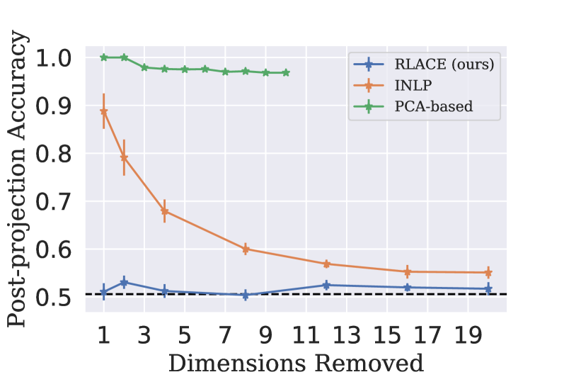
Figure 2: Gender prediction accuracy after bias-removal projection against the dimensionality of the neutralized subspace for INLP and R-LACE , on GloVe representations (Experiment § 5.1). Error bars are standard deviations.

In Ravfogel et al. (2020) it was shown that high-dimensional representation space tends to be (approximately) linearly separable by multiple orthogonal linear classifiers. This led Ravfogel et al. (2020) to the hypothesis that multiple directions are needed in order to fully capture the gender concept. Our results, in contrast, show that there is a $1$-dimensional subspace whose neutralization exhaustively removes the gender concept.

Importantly, as expected with a linear information removal method, non-linear classifiers are still able to recover gender: both RBF-SVM and a ReLU MLP with 1 hidden layer of size 128 predict gender with above 90% accuracy. We repeat the recommendation of Ravfogel et al. (2020): when using linear-removal methods, one should be careful to only feed the result to linear classifiers (such as the last layer of a neural network).

Clustering by Gender.

How does R-LACE influence the geometry of representation space? We perform PCA of the GloVe representations, and color the points by gender, both on the original representations, and after 1-rank gender-removal projection. As can be seen in Fig. 1, the original representation space is clustered by gender, and this clustering significantly decreases post-projection. See § B.7 for a quantitative analysis of this effect.

Word Association Tests.

	WEAT’s $d$ $\downarrow$	$p$-value
Math-art.
Original	1.57	0.000
PCA	1.56 $\pm$ 0.00	0.000 $\pm$ 0.000
RLACE	0.80 $\pm$ 0.01	0.062 $\pm$ 0.002
INLP	1.10 $\pm$ 0.10	0.016 $\pm$ 0.009
Professions-family.
Original	1.69	0.000
PCA	1.69 $\pm$ 0.00	0.000 $\pm$ 0.000
RLACE	0.78 $\pm$ 0.01	0.072 $\pm$ 0.003
INLP	1.15 $\pm$ 0.07	0.007 $\pm$ 0.003
Science-art.
Original	1.63	0.000
PCA	1.63 $\pm$ 0.00	0.000 $\pm$ 0.000
RLACE	0.77 $\pm$ 0.01	0.073 $\pm$ 0.003
INLP	1.03 $\pm$ 0.11	0.022 $\pm$ 0.016

Table 1: WEAT bias association results.

Caliskan et al. (2017) introduced the Word Embedding Association Test (WEAT), a measure for the association of similarity between male and female related words and stereotypically gender-biased professions. The test examines, for example, whether a group of words denoting STEM professions is more similar, in average, to male names than to female ones. We measure the association between Female and Male names and (1) career and family-related terms; (2) Art and Mathematics words; (3) Artistic and Scientific Fields. We report the test statistic, WEAT’s $d$ (see Caliskan et al. (2017) for more details), and the $p$-values after rank-$1$ projections in Tab. 1. R-LACE is most effective in decreasing biased associations to nearly nonsignificant $p$-values.

Influence on Semantic Content.

Does R-LACE damage the semantic content of the embeddings? We run SimLex-999 (Hill et al., 2015), a test that measures the quality of the embedding space by comparing word similarity in that space to a human notion of similarity. The test is composed of pairs of words, and we calculate the Pearson correlation between the cosine similarity before and after projection, and the similarity score that humans gave to each pair. Similarly to Ravfogel et al. (2020), we find no significant influence on correlation to human judgement, from 0.399 for the original vectors, to 0.392 after rank-1 projection and 0.395 after 1 iteration of INLP. See § B.8 for the neighbors of randomly-chosen words before and after R-LACE.

5.2 Deep Classification

Setting	Accuracy (gender) $\downarrow$	Accuracy (Profession) $\uparrow$	$\mathrm{GAP}_{\text{Male},y}^{\mathrm{TPR},\mathrm{RMS}}\downarrow$	$\sigma_{(\mathrm{GAP}^{\mathrm{TPR}},\%\text{Women})}\downarrow$
BERT-frozen	99.32	79.14	0.145	0.813
BERT-frozen+ RLACE (rank 1)	52.48	78.86	0.109	0.680
BERT-frozen+ RLACE (rank 100)	52.77	77.28	0.102	0.615
BERT-frozen+ INLP (rank 1)	98.98	79.09	0.137	0.816
BERT-frozen+ INLP (rank 100)	53.21	71.94	0.099	0.604
BERT-finetuned	96.89 $\pm$ 1.01	85.12 $\pm$ 0.08	0.123 $\pm$ 0.011	0.810 $\pm$ 0.023
BERT-finetuned+ RLACE (rank 1)	54.59 $\pm$ 0.66	85.09 $\pm$ 0.07	0.117 $\pm$ 0.011	0.794 $\pm$ 0.025
BERT-finetuned+ RLACE (rank 100)	54.33 $\pm$ 0.36	85.04 $\pm$ 0.09	0.115 $\pm$ 0.014	0.792 $\pm$ 0.025
BERT-finetuned+ INLP (rank 1)	93.52 $\pm$ 1.42	85.12 $\pm$ 0.08	0.122 $\pm$ 0.011	0.808 $\pm$ 0.024
BERT-finetuned+ INLP (rank 100)	53.04 $\pm$ 0.97	84.98 $\pm$ 0.06	0.113 $\pm$ 0.009	0.797 $\pm$ 0.027
BERT-adv (MLP adversary)	99.57 $\pm$ 0.05	84.87 $\pm$ 0.11	0.128 $\pm$ 0.004	0.840 $\pm$ 0.015
BERT-adv (Linear adversary)	99.23 $\pm$ 0.09	84.92 $\pm$ 0.12	0.124 $\pm$ 0.005	0.827 $\pm$ 0.012
Majority	53.52	30.0	-	-

Table 2: Fair classification results, deep profession classification (Experiment § 5.2). We consider the original representations of the pretrained and finetuned models (BERT-frozenand BERT-finetuned), and the same representations after INLP and RLACE. We also consider two adversarially-finetuned models (BERT-adv), that serve as baselines. For each model, we record the ability to recover gender, main-task (profession prediction) accuracy, the true-positive-rate gap ($\mathrm{GAP}_{\text{Male},y}^{\mathrm{TPR},\mathrm{RMS}}$) and the correlation between this gap and the bias that is reflected in the data ($\sigma_{(\mathrm{GAP}^{\mathrm{TPR}})}$).

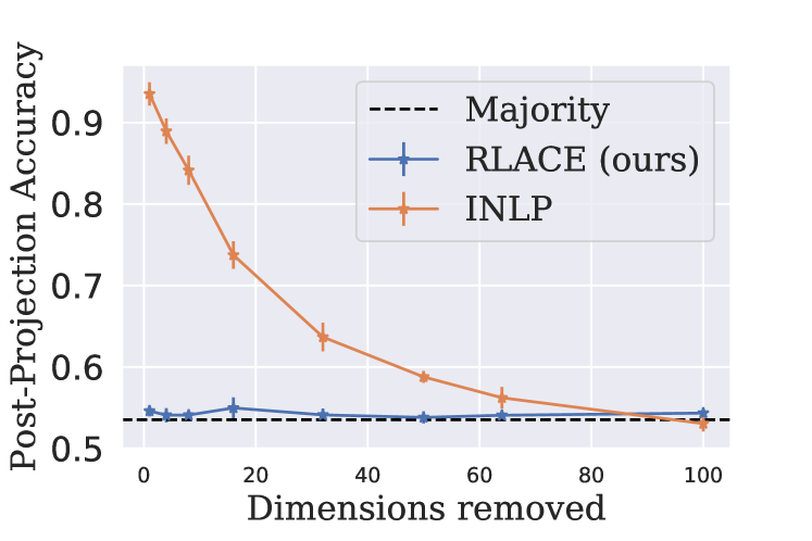
Figure 3: Gender prediction accuracy after bias-removal projection against the dimensionality of the neutralized subspace, for INLP and R-LACE , finetuned BERT representations (Experiment § 5.2).

We proceed to evaluate the impact of R-LACE on deep classifiers with a focus on the fairness of the resulting classifiers. De-Arteaga et al. (2019) released a large dataset of short biographies collected from the web annotated for both binary gender and profession. We embed each biography with the [CLS] representation in the last layer of BERT, run Alg. 1 to remove gender information from the [CLS] , and then evaluate the performance of the model, after the intervention, on the main task of profession prediction.

Main-Task Classifiers.

We consider several deep profession classifiers:

• A multiclass logistic regression profession classifier over the frozen representations of pre-trained BERT (BERT-frozen);

• A pretrained BERT model finetuned to the profession classification task (BERT-finetuned);

• A pretrained BERT model finetuned to the profession classification task, trained adversarially for gender removal with the gradient-reversal layer method of Ganin and Lempitsky (2015) (BERT-adv). We consider (1) a linear adversray (2) an MLP adversary with 1-hidden-layer of size 300 and ReLU activations.

We run Alg. 1 on the representations of BERT-frozen and BERT-finetuned , while BERT-adv is the commonly used way to remove concepts, and is used as a baseline. We report the results of 5 runs with random initializations. Before running Alg. 1, we reduce the dimensionality of the representations to 300 using PCA. We finetune the linear profession-classification head following the projection. See § B.6 for more details on our experimental setting.

Downstream Fairness Evaluation.

To measure the bias in a classifier, we follow De-Arteaga et al. (2019) and use the TPR-GAP measure, which quantifies the bias in a classifier by considering the difference (GAP) in the true positive rate (TPR) between individuals with different protected attributes (e.g. gender, race). We use the notation $\mathrm{GAP}_{z,y}^{\mathrm{TPR}}$ to denote the TPR-GAP in some main-class label $y$ (e.g. “nurse” prediction) for some protected group $z$ (e.g. “female”), we also consider $\mathrm{GAP}_{z}^{\mathrm{TPR},\mathrm{RMS}}$, the RMS of the TPR-GAP across all professions for a protected group $z$. See formal definitions in § B.6 and De-Arteaga et al. (2019). To calculate the relation between the bias the model exhibits and the bias in the data, we also calculate $\sigma_{(\mathrm{GAP}^{\mathrm{TPR}},\%\text{Women})}$, the correlation between the TPR gap in a given profession and the percentage of women in that profession.

The results are summarized in Tab. 2. R-LACE effectively hinders the ability to predict gender from the representations using a rank-$1$ projection, while INLP requires about 100 iterations (Fig. 3). Both methods have a moderate negative impact on the main task of profession prediction in the finetuned model, while in the frozen model, INLP—but not R-LACE—also significantly damages the main-task (from 79.14% to 71.94% accuracy). Bias, as measured by $\mathrm{GAP}_{z,y}^{\mathrm{TPR},\mathrm{RMS}}$ is mitigated by both methods to a similar degree. For the finetuned model, the decrease in $\sigma_{(\mathrm{GAP}^{\mathrm{TPR}},\%\text{Women})}$ is modest for all methods.

Interestingly, the adversarially finetuned models (BERT-adv)—both with a linear and an MLP adversary—does not show decreased bias according to $\mathrm{GAP}_{z,y}^{\mathrm{TPR},\mathrm{RMS}}$, and do not hinder the ability to predict gender at all. Besides the effectiveness of R-LACE for selective information removal, we conclude that the connection between the ability to predict gender from the representation, and the TPR-GAP metric, is not clear cut, and requires further study, as has been noted recently (Goldfarb-Tarrant et al., 2021; Orgad et al., 2022).

5.3 Erasing Concepts in Image Data

Our empirical focus is concept removal in textual data. Visual data, however, has the advantage of being able to clearly inspect the influence of R-LACE on the input. To qualitatively assess this effect, we use face images from the CelebsA dataset (Yang et al., 2015), which is composed of faces annotated with different concepts, such as “sunglasses” and “smile”. We downscaled all data to 50 over 50 grey-scale images, flatten them to 2,500-dimensional vectors, and run our method on the raw pixels (aiming to prevent a linear classifier to classify, for instance, whether a person has sunglasses based on the pixels of their image). We experimented with the following concepts: “glasses”, “smile”, “mustache”, “beard”, “bald” and “hat”.

Results.

See Fig. 4 and § B.9 for randomly-sampled outputs. In all cases, a rank-$1$ linear projection is enough to remove the ability to classify attributes (classification accuracy of less than 1% above majority accuracy). The intervention changed the images by focusing on the features one would expect to be associated with the concepts of interest; for example, adding “pseudo sun-glasses” to all images (for “glasses”) and blurring the facial features around the mouth (for “smile”). Since the intervention is constrained to be a projection, it is limited in expressivity, and it often zeros-out pixels to simulate a concept of interest, such as sunglasses. These results suggest that very simple style transfer of images does not always necessitate deep architectures, such as Style GAN (Karras et al., 2019).

6 Related Work

Concept removal is predominantly based on adversarial approaches (Goodfellow et al., 2014), which were extensively applied to bias mitigation problems (Ganin and Lempitsky, 2015; Edwards and Storkey, 2016; Chen et al., 2018; Xie et al., 2017; Zhang et al., 2018; Wang et al., 2021). However, those methods are notoriously unstable, and were shown by Elazar and Goldberg (2018) to be non-exhaustive: residual bias often still remains after apparent convergence. Linear information removal method was pioneered by Bolukbasi et al. (2016), who used PCA to identify “gender subspace” spanned by a few presupposed “gender directions”. Following the criticism of Gonen and Goldberg (2019), several works have proposed alternative linear formulations (He et al., 2020; Dev and Phillips, 2019; Ravfogel et al., 2020; Dev et al., 2021; Kaneko and Bollegala, 2021).

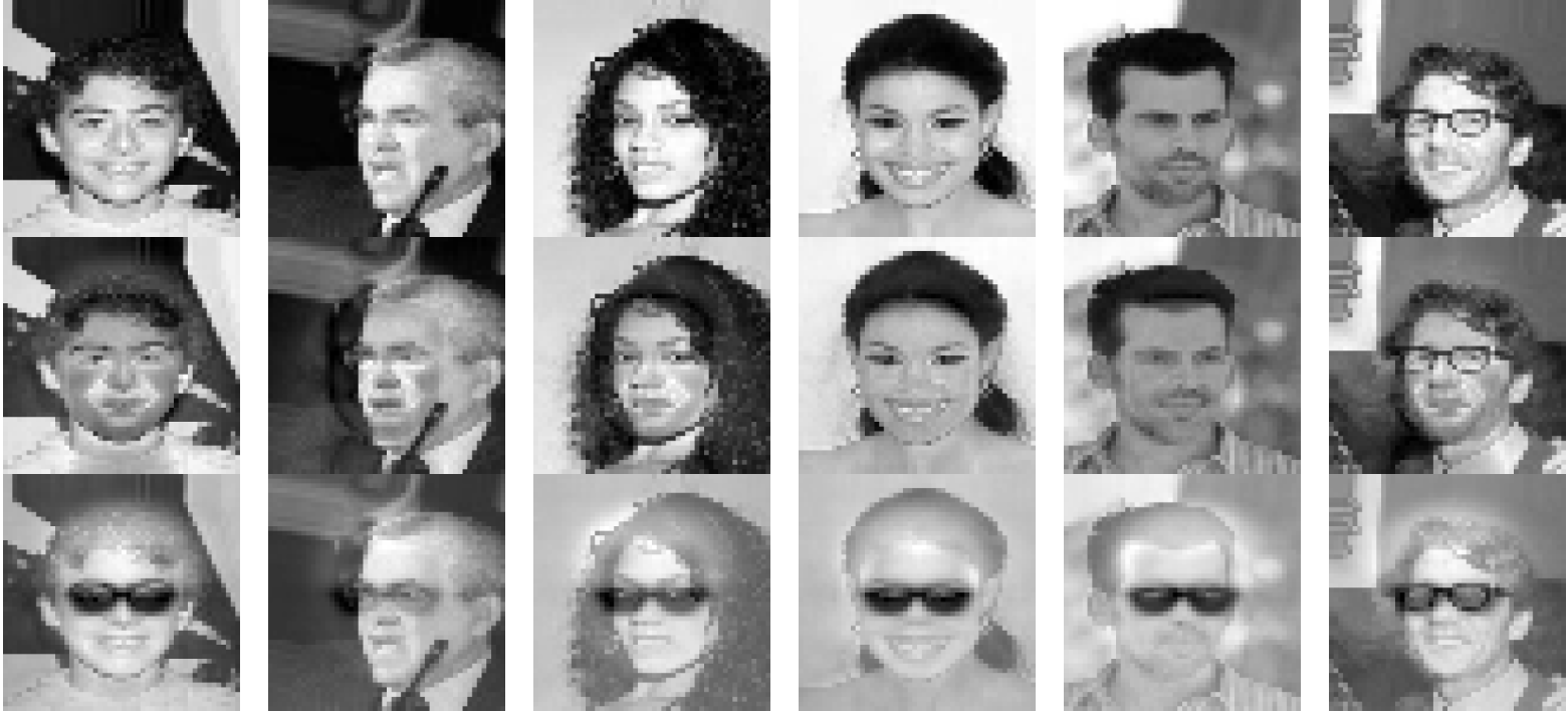
Figure 4: Application of R-LACE on the raw pixels of image data, from top to bottom we present the original images and the same images after a rank-$1$ projection, for the concepts “smile” and “glasses”.

Concurrent to this work, spectral removal of information (a special case of the Rayleigh-quotient loss, § 2) was studied in Shao et al. (2022), who projected out the directions that explain most of the covariance between the representations and the protected attribute, and also proposed a kernalization of the Rayleigh-quotient objective. Closest to our work are Sadeghi et al. (2019) and Sadeghi and Boddeti (2021), who studied a different linear adversarial formulation and quantified the inherent trade-offs between information removal and main-task performance. Their analysis is focused on the special case of linear regression, and they considered a general linear adversary (which is not constrained to an orthogonal projection – making it more expressive, but less interpetable). Finally, Haghighatkhah et al. (2021) provide a thorough theoretical analysis of the problem of preventing classification through an orthogonal projection, and provide a constructive proof for optimality against SVM adversaries.

Beyond bias mitigation, concept subspaces have been used as an interpretability tool (Kim et al., 2018), for causal analysis of NNs (Elazar et al., 2021; Ravfogel et al., 2021), and for studying the geometry of their representations (Celikkanat et al., 2020; Gonen et al., 2020; Hernandez and Andreas, 2021). Our linear concept removal objective is different from subspace clustering (Parsons et al., 2004), as we focus on hindering the ability to linearly classify the concept, and do not assume that the data lives in a linear or any low-dimensional subspace.

7 Conclusion

We have formulated the task of erasing concepts from the representation space as a constrained version of a general minimax game. In the constrained game, the adversary is limited to a fixed-rank orthogonal projection. This constrained formulation allows us to derive closed-form solutions to this problems for certain objectives, and propose a convex relaxation which works well in practice for others. We empirically show that the relaxed optimization recovers a single dimensional subspace whose removal is enough to mitigate linearly-present gender concepts.

The method proposed in this work protects against linear adversaries. Effectively removing non-linear information while maintaing the advantages of the constrained, linear approach remains an open challenge.

Appendix A Pseudocode

Algorithm 1 Relaxed Linear Adversarial Concept Erasure (R-LACE)

  Input:

  data $X\in\mathbb{R}^{N\times D}$

  labels $\boldsymbol{y}$

  Loss $\ell$

  Projection rank $k$

  outer loops $T$

  inner loops $M$

  Output:

  A projection matrix $P$ that neutralizes a rank-$k$ subspace

  Initialization:

  Initialize predictor ${\boldsymbol{\theta}}\in\mathbb{R}^{D}$ randomly.

  Initialize adversary $P\in\mathbb{R}^{D\times D}$ randomly.

  Run adversarial game:

  for $i=1$ to $T$ do

     for $j=1$ to $M$ do

        /* Gradient descent on ${\boldsymbol{\theta}}$

        ${\boldsymbol{\theta}}\leftarrow$SGDUpdate $\left(\frac{\partial\ell(\boldsymbol{y},XP{\boldsymbol{\theta}})}{\partial{\boldsymbol{\theta}}}\right)$

     end for

     for $j=1$ to $M$ do

        /* Projected gradient ascent on $P$

        $P\leftarrow$SGDUpdate $\left(\frac{-\partial\ell(\boldsymbol{y},XP{\boldsymbol{\theta}})}{\partial P}\right)$

        $P\leftarrow\frac{1}{2}(P+P^{\top})$ //Ensure $P$ is symmetric

        $P\leftarrow\texttt{FantopeProjection}(P,k)$ //Project on the Fantope using Lemma B.1

     end for

  end for

  /* Perform SVD to get a proper orthogonal projection matrix that reduces the rank by $k$

  $U,D=$ spectralDecomposition($P$)

  $P\leftarrow{U[:-k,:]}^{\top}U[:-k,:]$

  return $P$

Appendix B Appendices

B.1 Ethical Considerations

The empirical experiments in this work involve the removal of binary gender information from a pre-trained representation. Beyond the fact that gender a non-binary concept, this task may have real-world applications, in particular such that relate to fairness. We would thus like remind the readers to take the results with a grain of salt and be extra careful when attempting to deploy methods such as the one discussed here. Regardless of any proofs, care should be taken to measure the effectiveness of the approach in the context in which it is to be deployed, considering, among other things, the exact data to be used, the exact fairness metrics under consideration, the overall application, and so on. We urge practitioners not to regard this method as a “solution” to the problem of bias in neural models, but rather as a preliminary research effort towards mitigating certain aspects of the problem. Unavoidably, we make use a limited set of datasets in our experiments, and they do not reflect all the subtle and implicit ways in which gender bias is manifested. As such, it is likely that different forms of bias still exist in the representations following the application of our method. We hope that followup works would illuminate some of these shortcomings.

Furthermore, our method targets a very specific technical definition of bias, quantified by the ability to linearly predict the sensitive information. The method is not expected to be robust to nonlinear adversaries, or generally other ways to quantify bias.

B.2 Rayleigh-quotient

In this appendix, we provide a derivation of the equilibrium point of the linear adversarial game for objectives that can be cast as Rayleigh quotient maximization (§ 3.2). We prove that these objective, the optimal projection of rank $k$ neutralizes the subsapce spanned by the $k$-best ${\boldsymbol{\theta}}_{1},\dots,{\boldsymbol{\theta}}_{k}$ — i.e., the first $k$ directions that maximize the Rayleigh quotient.

See 3.2

Proof.

First, we manipulate the objective

$$\frac{({\boldsymbol{\theta}}P)^{\top}A({\boldsymbol{\theta}}P)}{({\boldsymbol{\theta}}P)^{\top}({\boldsymbol{\theta}}P)} =\frac{({\boldsymbol{\theta}}P)^{\top}V^{\top}\Lambda V({\boldsymbol{\theta}}P)}{({\boldsymbol{\theta}}P)^{\top}({\boldsymbol{\theta}}P)}$$ (19)

$$=\frac{({\boldsymbol{\theta}}P)^{\top}V^{\top}\Lambda V({\boldsymbol{\theta}}P)}{({\boldsymbol{\theta}}P)^{\top}V^{\top}V({\boldsymbol{\theta}}P)}$$ (20)

$$=\frac{(V{\boldsymbol{\theta}}P)^{\top}\Lambda(V{\boldsymbol{\theta}}P)}{(V{\boldsymbol{\theta}}P)^{\top}(V{\boldsymbol{\theta}}P)}$$ (21)

Define $$\tilde{{\boldsymbol{\theta}}}=V{\boldsymbol{\theta}}$$. (22)

$$=\frac{(\tilde{{\boldsymbol{\theta}}}P)^{\top}\Lambda(\tilde{{\boldsymbol{\theta}}}P)}{(\tilde{{\boldsymbol{\theta}}}P)^{\top}(\tilde{{\boldsymbol{\theta}}}P)}$$ (23)

$$=\frac{\sum_{d=1}^{D}\lambda_{d}\cdot(\tilde{{\boldsymbol{\theta}}}P)_{d}^{2}}{\sum_{d=1}^{D}(\tilde{{\boldsymbol{\theta}}}P)_{d}^{2}}$$ (24)

Since 24 is scale-invariant, we may assume $\tilde{{\boldsymbol{\theta}}}P$ is a unit vector.

Upper Bound.

We first argue for an upper bound on the objective. For any orthogonal projection matrix $P_{0}$ of rank $k$, we have

$$\max_{\tilde{{\boldsymbol{\theta}}}\in\mathbb{R}^{D}} \min_{\begin{subarray}{c}P\in\mathbb{R}^{D\times D}\\ \text{s.t. }P^{2}=P=P^{\top}\end{subarray}}\sum_{d=1}^{D}\lambda_{d}\cdot(\tilde{{\boldsymbol{\theta}}}P)_{d}^{2}$$ (25)

$$\leq\max_{\tilde{{\boldsymbol{\theta}}}\in\mathbb{R}^{D}}\sum_{d=1}^{D}\lambda_{d}\cdot(\tilde{{\boldsymbol{\theta}}}P_{0})_{d}^{2}$$ (26)

subject to the constraint that $||\tilde{{\boldsymbol{\theta}}}P_{0}||_{2}^{2}=1$. To solve the max, let $d^{\star}$ be the smallest value in $\{1,\ldots,D\}$ such that $\boldsymbol{e}_{d^{\star}}\in\textsf{range}(P_{0})$ where we use $\boldsymbol{e}_{i}$ to denote the $i^{\text{th}}$ natural basis vector. Thus, we have

$$\max_{\tilde{{\boldsymbol{\theta}}}\in\mathbb{R}^{D}}\sum_{d=1}^{D}\lambda_{d}\cdot(\tilde{{\boldsymbol{\theta}}}P_{0})_{d}^{2} =\sum_{d=1}^{D}\lambda_{d}\cdot(\boldsymbol{e}_{d^{\star}})_{d}^{2}$$ (27)

$$=\lambda_{d^{\star}}$$ (28)

Minimizing over $P_{0}$, we find that the smallest value is achieved by $\tilde{{\boldsymbol{\theta}}}P=\boldsymbol{e}_{k+1}$ and the value of the objective is $\lambda_{k+1}$. To backsolve for ${\boldsymbol{\theta}}$, we note that

$$\boldsymbol{e}_{k+1}=V{\boldsymbol{\theta}}P$$ (29)

which is true when ${\boldsymbol{\theta}}^{\star}=\boldsymbol{v}_{k+1}$ and $P^{\star}=I-\sum_{d=1}^{D-k}\boldsymbol{v}_{d}\boldsymbol{v}_{d}^{\top}$.

Lower Bound.

Now, for any $\tilde{{\boldsymbol{\theta}}_{0}}$, we have the following lower bound:

$$\max_{\tilde{{\boldsymbol{\theta}}}\in\mathbb{R}^{D}}\min_{\begin{subarray}{c}P\in\mathbb{R}^{D\times D}\\ \text{s.t. }P^{2}=P=P^{\top}\end{subarray}}\sum_{d=1}^{D}\lambda_{d}\cdot(\tilde{{\boldsymbol{\theta}}}P)_{d}^{2}$$ (30)

$$\geq\min_{\begin{subarray}{c}P\in\mathbb{R}^{D\times D}\\ \text{s.t. }P^{2}=P=P^{\top}\end{subarray}}\sum_{d=1}^{D}\lambda_{d}\cdot(\tilde{{\boldsymbol{\theta}}_{0}}P)_{d}^{2}$$ (31)

Now, we consider minimizing $P$ when $\tilde{{\boldsymbol{\theta}}_{0}}$ can only take values from the finite subset $\{\boldsymbol{e}_{1},\ldots,\boldsymbol{e}_{k+1}\}$. This is equivalent to minimizing over $P$ when we have ${\boldsymbol{\theta}}_{0}\in\{\boldsymbol{v}_{1},\ldots,\boldsymbol{v}_{k+1}\}$. The $P^{\star}$ that minimizes over this collection is

$$P^{\star}=I-\sum_{d=1}^{D-k}\boldsymbol{v}_{d}\boldsymbol{v}_{d}^{\top}$$ (32)

This is true as $\textsf{null}\left(P\right)=\texttt{span}\left(\{\boldsymbol{v}_{1},\ldots,\boldsymbol{v}_{k}\}\right)$ which zeros out the elements of the collection that achieve the highest values of the objective in this collection, i.e. $\{\boldsymbol{v}_{1},\ldots,\boldsymbol{v}_{k}\}$. Plugging in $P^{\star}$, we get ${\boldsymbol{\theta}}^{\star}=\boldsymbol{v}_{k+1}$ and the value of the objective is $\lambda_{k+1}$.

Putting it Together.

Given that we have upper and lower bounded the problem with $\lambda_{k+1}$, we conclude the solution is as stated in the theorem. ∎

B.3 Linear Regression

In this appendix, we provide a derivation of the equilibrium point of the linear adversarial game in the linear regression case (§ 3.1). We show that the optimal projection is of rank 1, and that it neutralizes the covariance direction $X\boldsymbol{y}$. See 3.1

Proof.

Let $P=I-\frac{\boldsymbol{v}\boldsymbol{v}^{\top}}{\boldsymbol{v}^{\top}\boldsymbol{v}}$ be an arbitrary orthogonal projection matrix, where span($\boldsymbol{v})$ is the rank-1 concept subspace that is neutralized. For every choice of $\boldsymbol{v}$, the optimal ${\boldsymbol{\theta}}$ is ${\boldsymbol{\theta}}={({(XP)}^{\top}XP)}^{-1}X^{\top}y={(PX^{\top}XP)}^{-1}PX^{\top}\boldsymbol{y}:=CX^{\top}\boldsymbol{y}$, where $C$ is the inverse (or pseudoinverse) matrix. Consider the choice $\boldsymbol{v}:=X^{\top}\boldsymbol{y}$. For this choice, the objective is evaluated to $\frac{1}{2}{||\boldsymbol{y}-XP{(PX^{\top}XPw)}^{-1}PX^{\top}\boldsymbol{y}||}^{2}$. Since, by definition, $P$ projects to the nullspace of $X^{\top}\boldsymbol{y}$, we have $PX^{\top}\boldsymbol{y}=\vec{0}$ and the objective is then evaluated to $\frac{1}{2}{||\boldsymbol{y}||}^{2}$. Thus, the objective is the variance of $\boldsymbol{y}$, regardless or the value of ${\boldsymbol{\theta}}$. Note also that the adversary cannot improve over this choice for $P$, since regardless of the choice of $P$, the predictor can always choose ${\boldsymbol{\theta}}=\vec{0}$ and get an objective value of $Var(\boldsymbol{y})$ – so this is an upper bound for the objective.

∎

B.4 Optimizing the Relaxed Objective

In this appendix, we describe the optimization of the relaxed objective § 3.4.

B.4.1 Alternate Optimization with Projected Gradient Descent

To optimize the relaxed objective 18, we perform alternate minimization and maximization over ${\boldsymbol{\theta}}$ and $P$, respectively. ${\boldsymbol{\theta}}$ is updated with a regular gradient descent:

$${\boldsymbol{\theta}}_{t+1}\leftarrow{\boldsymbol{\theta}}_{t}-\alpha_{t}\nabla_{{\boldsymbol{\theta}}}\sum_{n=1}^{N}\ell\left(y_{n},g^{-1}\!\left({\boldsymbol{\theta}}^{\top}P\boldsymbol{x}_{n}\right)\right)$$

While $P$ is updated with projected gradient ascent:

$$P_{t+1}\leftarrow\Pi_{\mathcal{F}_{k}}\left(P_{t}+\alpha_{t}\nabla_{P}\sum_{n=1}^{N}\ell\left(y_{n},g^{-1}\!\left({\boldsymbol{\theta}}^{\top}P\boldsymbol{x}_{n}\right)\right)\right)$$

where $\alpha_{t}$ is the learning rate, and $\Pi_{\mathcal{F}_{k}}$ is the projection to the Fantope, given in Vu et al. (2013). The following lemma describes how to calculate that projection:

Lemma B.1 (Restated from Vu et al. (2013)).

Let $\mathcal{F}_{k}$ be the $k$-dimensional fantope; see 17, and let $P=\sum_{d=1}^{D}\lambda_{d}\boldsymbol{v}_{d}\boldsymbol{v}_{d}^{\top}$ be the eigendecomposition of $P$ where $\lambda_{d}$ is $P$’s $d$^th eigenvalue and $\boldsymbol{v}_{d}$ is its corresponding eigenvector. The projection of $P$ onto the fantope is given by $\Pi_{\mathcal{F}_{k}}(P)=\sum_{d=1}^{D}\lambda_{d}^{+}(\gamma)\cdot\boldsymbol{v}_{d}\boldsymbol{v}_{d}^{\top}$, where $\lambda_{d}^{+}(\gamma)=\min\left(\max(\lambda_{d}-\gamma,0),1\right)$ and $\gamma$ satisfies the equation $\sum_{d=1}^{D}\lambda_{d}^{+}(\gamma)=k$.

The lemma specifies that finding the projection entails performing an eigendecomposition of $P$ and finding $\gamma$ that satisfies a set of monotonous, piece-wise linear equations. Since we can easily find $\gamma$ where $\sum_{d=1}^{D}\lambda_{d}^{+}(\gamma)>k$ and $\gamma$ where $\sum_{d=1}^{D}\lambda_{d}^{+}(\gamma)<k$, we can solve the system of equations using the bisection method.

Upon termination of the optimization process, we perform spectral decomposition of $P$, and return a projection matrix to the space spanned by the first $D-k$ eigenvectors (to ensure a proper orthogonal projection matrix that neutralizes a rank-$k$ subspace). The process is summarized in Alg. 1. The matrix $P$ can then be used to mitigate bias in the dataset $X$ by projecting $X\leftarrow XP$.

Convergence

Concave–convex adversarial problems have a unique Nash equilibrium under mild conditions (Pang and Razaviyayn, 2016), and there is a rich literature on efficient solution to these problems. However, Even for the concave–convex case, alternate optimization–as we employ–is not guaranteed to find that equilibrium, and is prone to problems such as rotational behavior (Nouiehed et al., 2019). Indeed, in our experiments, we witness such behavior: the objective does not converge smoothly. However, in all cases, when we run the algorithm for enough iterations and continuously evaluate the projection $P$ by fixing it, training ${\boldsymbol{\theta}}$ to convergence and evaluating it on the development set, we converge to an optimal $P$ (in the sense of ${\boldsymbol{\theta}}$ achieving majority-accuracy) at certain point. We then terminate the optimization and take that optimal $P$. Because of these positive results we opted for using vanilla alternate optimization, although more sophisticated algorithms, that do guarantee convergence to the equilibrium point, have also been developed for convex–concave games (Wang and Li (2020); Yoon and Ryu (2021), inter alia).

Also, note that due to the implicit function theorem and the concave–convex nature of the problem, for every fixed $P$, $\underset{{\boldsymbol{\theta}}\in\Theta}{\operatorname{argmin}}\,\,{\ell(\boldsymbol{y},XP{\boldsymbol{\theta}})}$ is an implicit function $h(P)$ of $P$ for some $h(\cdot)$, making 18 equivalent to the concave, non-adversarial problem $\underset{P\in\mathcal{F}_{k}}{\operatorname{argmax}}\,\,{h(P)}$, which is an “easy” and conventional concave problem. Calculating the function $h(\cdot)$ explicitly is computationally intensive, as it involves Hessian calculations, and efficiently optimizing it is an active area of research (Blondel et al., 2021).

B.5 Experimental Setting: Static Word Vectors

In this appendix, we describe the experimental setting in the static word vectors experiments § 5.1.

We conduct experiments on 300-dimensional uncased GloVe vectors. Following (Ravfogel et al., 2020), to approximate the gender labels for the vocabulary, we project all vectors on the $\overrightarrow{he}-\overrightarrow{she}$ direction, and take the $7,500$ most male-biased and female-biased words. Note that unlike (Bolukbasi et al., 2016), we use the $\overrightarrow{he}-\overrightarrow{she}$ direction only to induce approximate gender labels, but then proceed to measure the bias in various ways, that go beyond neutralizing just the $\overrightarrow{he}-\overrightarrow{she}$ direction.

We use the same train–dev–test split of Ravfogel et al. (2020), but discard the gender-neutral words (i.e., we cast the problem as a binary classification). We end up with a training set, evaluation set and test set of sizes 7,350, 3,150 and 4,500, respectively.

We run Alg. 1 for 50,000 iterations with the cross entropy loss, alternating between an update to the adversary and to the classifier after each iteration ($T=50,000,M=1$ in Alg. 1).

The inner optimization problem entailed in the Fantope projection operation is solved with the bisection method. We train with a simple SGD, with a learning rate of $0.005$, chosen by experimenting with the development set. We use a batch size of 128. After each 1000 batches, we freeze the adversary, train the classifier to convergence, and record its loss. Finally, we return the adversary which yielded the highest classification loss. In test time, we evaluate the ability to predict gender using logistic regression classifiers trained in Sklearn. For the dimensionality of the neutralized subspace, we experiment with the values $k=1\dots 20$ for INLP and R-LACE.̇ We perform 5 runs and report mean $\pm$ standard deviation.

B.6 Experimental Setting: Deep Classifiers

In this appendix, we describe the experimental setting in the deep classification experiments § 3.3.

We use the same train–dev–test split of the biographies dataset used by Ravfogel et al. (2020), resulting in training, evaluation and test sets of sizes 255,710, 39,369, and 98,344, respectively. We reduce the dimensionality of the representations to 300 using PCA, and for efficiency reasons, we run Alg. 1 on the first 100,000 training examples only (but test on all the test data).

We run Alg. 1 with a simple SGD optimization, with a learning rate of $0.005$ and a weight decay of $1e^{-4}$, chosen by experimenting with the development set. We use a batch size of 256, and again choose the adversary which yielded highest classification loss. For the dimensionality of the neutralized subspace, we run R-LACE and INLP with $k=1\dots 100$. We perform 5 runs of the entire experimental pipeline (classifier training, INLP and R-LACE
) and report mean $\pm$ standard deviation.

Classifier training

We experiment with several deep profession classifiers, as detailed in § 3.3. For BERT-frozen, we use the HuggingFace implementation (Wolf et al., 2020). For BERT-finetuned  we finetune the pre-trained BERT on the profession classification task, using a SGD optimizer with a learning rate of $0.0005$, weight decay of $1e^{-6}$ and momentum of 0.9. We train for 30,000 batches of size 10 and choose the model which achieved lowest loss on the development set. For BERT-adv, we perform the same training procedure, but add an additional classification head which is trained to predict gender, and whose gradient is reversed (Ganin and Lempitsky, 2015). This procedure should create an encoder which generates hidden representations which are predictive of the main task, but are not predictive of gender. The adversary always converged to a low gender classification accuracy (below $55\%$), which is commonly interpreted as a success of the removal process.

Fairness Measure: TPR-GAP

We formally describe the fairness measures used in § 5.2.

The TPR-GAP is tightly related to the notion of fairness by equal opportunity (Hardt et al., 2016): a fair binary classifier is expected to show similar success in predicting the task label $\boldsymbol{y}$ for the two populations, when conditioned on the true class. Formally, let $Z$ is a random variable denoting binary protected attribute, $z$ and $z^{\prime}$ denote its two values, and let $Y$ denote a random variable describing the main-task label, and similarly let $\widehat{Y}$ be a random variable denoting the model’s prediction on the main task (e.g. profession). TPR between a main-task label $y$ and a protected group $z$, and the gap in the TPR, are defined as follows (De-Arteaga et al., 2019):

$$\mathrm{TPR}_{z,y}= p(\widehat{Y}=y\mid Z=\textsl{z},Y=y)$$ (33)

$$\mathrm{GAP}_{z,y}^{\mathrm{TPR}}= \mathrm{TPR}_{z,y}-\mathrm{TPR}_{z^{\prime},y}$$ (34)

We also consider the root-mean square of $GAP_{z,y}^{TPR}$ over all main-class labels, to get a single per-gender bias score:

$$\mathrm{GAP}_{z}^{\mathrm{TPR},\mathrm{RMS}}=\sqrt{\frac{1}{|C|}\sum_{y\in C}(\mathrm{GAP}_{z,y}^{\mathrm{TPR}})^{2}}$$ (35)

where $C$ is the set of all labels (in our case, professions).

B.7 V-Measure

To quantify the effect of our intervention on the GloVe representation sapce in § 5.1, we perform $K$-means clustering with different values of $K$, and use $V-$measure (Rosenberg and Hirschberg, 2007) to quantify the association between cluster identity and the gender labels, after a projection that removes rank-$1$ subspace. The results are presented in Fig. 5. $V$-measure for the original representations is 1.0, indicating a very high alignment between cluster identity and gender label. The score drastically drops after a rank-$1$ relaxed projection, while INLP projection and the PCA-based method of (Bolukbasi et al., 2016) have a smaller effect.

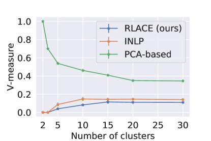
Figure 5: V-measure between gender labels and cluster identity, for different numbers of clusters on the X axis (lower values are better). Error bars are standard deviations from 10 random runs.

B.8 Influence on Neighbors in Embedding Space

In § 5.1, we showed that the SimLex999 test does not find evidence to damage that our intervention causes to the GloVe embedding space. To qualitatively demonstrate this, we provide in Tab. 3 the closest-neighbors to 15 randomly-sampled words from the vocabulary, before and after our intervention.

Word	Neighbors before	Neighbors after
history	literature, histories, historical	literature, histories, historical
1989	1991, 1987, 1988	1991, 1987, 1988
afternoon	saturday, evening, morning	sunday, evening, morning
consumers	buyers, customers, consumer	buyers, customers, consumer
allowed	allowing, allow, permitted	allowing, allow, permitted
leg	thigh, knee, legs	thigh, knee, legs
manner	therefore, regard, thus	means, regard, thus
vinyl	metal, lp, pvc	metal, lp, pvc
injury	injured, accident, injuries	injured, accident, injuries
worried	afraid, concerned, worry	afraid, concerned, worry
dishes	cooking, cuisine, dish	meals, cuisine, dish
thursday	monday, tuesday, wednesday	monday, tuesday, wednesday
sisters	brothers, daughters, sister	daughters, brothers, sister
wants	decides, thinks, knows	decides, thinks, knows
covering	cover, covered, covers	cover, covered, covers

Table 3: Neighbors to random words in GloVe space before and other rank-1 R-LACE projection.

B.9 Additional results on the CelebsA dataset

We present here randomly-sampled outputs for the 6 concepts we experimented with: “glasses”, “smile”, “mustache”, “beard”, “bald” and “hat” (Experiment § 5.3).

Figure 6: Glasses

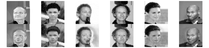
Figure 7: Smile

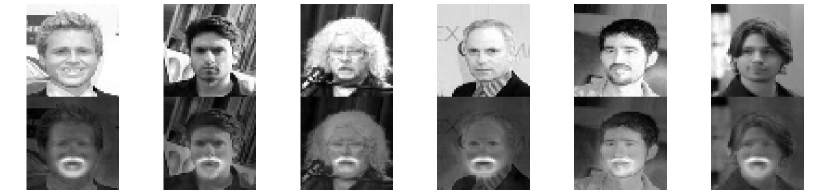
Figure 8: Mustache

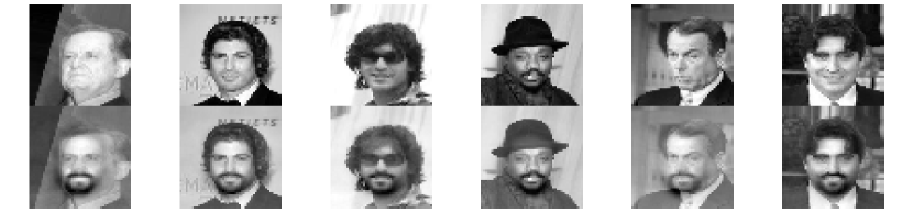
Figure 9: Beard

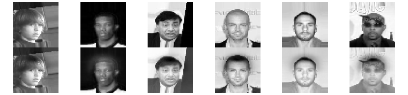
Figure 10: Bald

Figure 11: Hat

B.10 Relaxation Quality

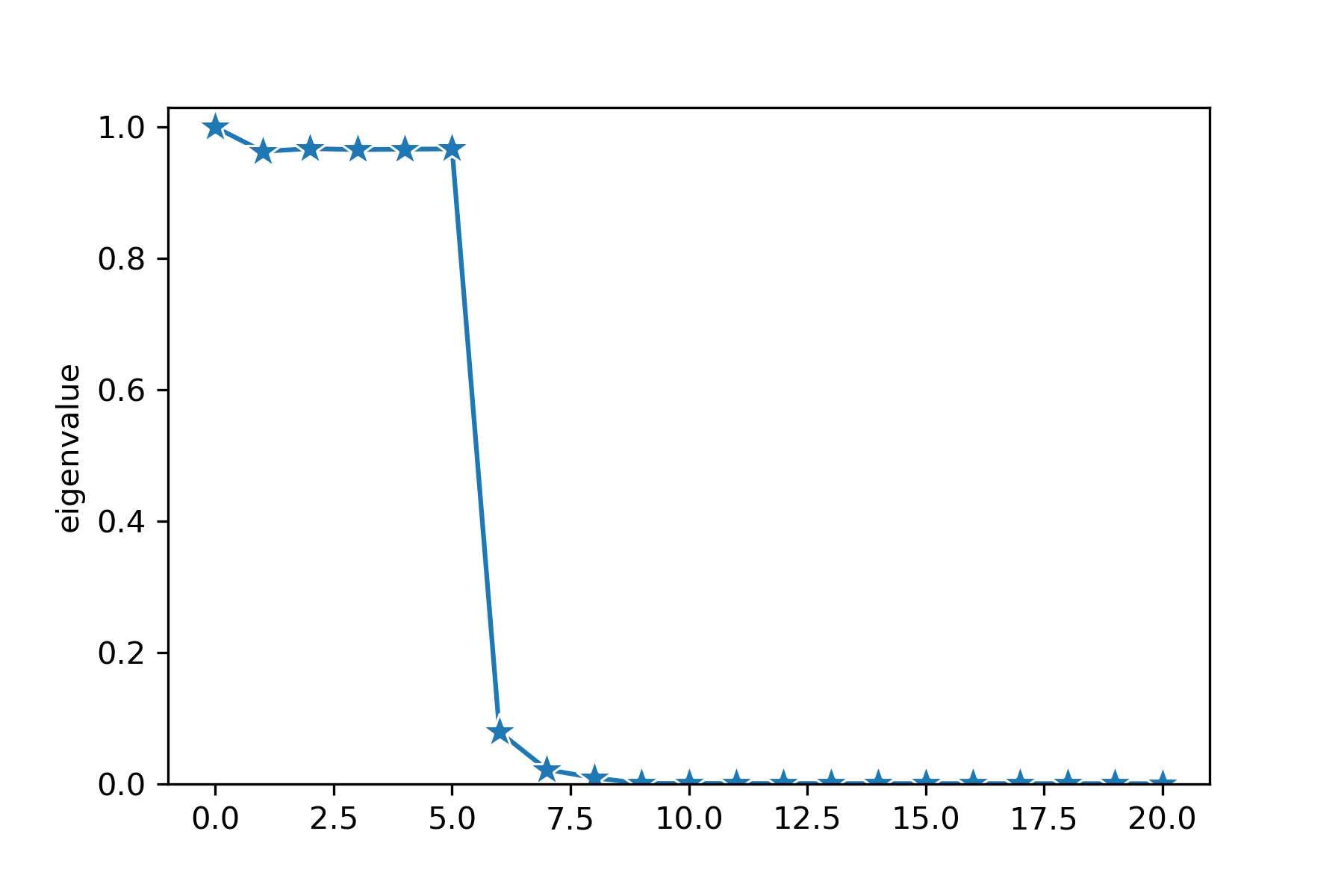
Figure 12: Eigenvalues spectrum of the output of the relaxed optimization when running Alg. 1 with $k=6$.

To what extent the optimization of the relaxed objective 18 results in a matrix $P$ that is a valid a rank-$k$ orthogonal projection matrix? recall that orthogonal projection matrix have binary eigenvalues: all eigenvalues are either zeros or ones, and their sum is the rank of the matrix. In Fig. 12, we present the eigenvalues spectrum of $P$ when we run Alg. 1 with $k=6$ on the static word-embeddings dataset (§ 5.1). We find that the top $6$ eigenvalues are indeed close to 1, and the rest are close to 0—suggesting the approximation is tight: the resulting matrix is close to a valid rank-$k$ orthogonal projection matrix.

References

- Blondel et al. (2021) Mathieu Blondel, Quentin Berthet, Marco Cuturi, Roy Frostig, Stephan Hoyer, Felipe Llinares-López, Fabian Pedregosa, and Jean-Philippe Vert. 2021. Efficient and modular implicit differentiation.
- Bolukbasi et al. (2016) Tolga Bolukbasi, Kai-Wei Chang, James Y. Zou, Venkatesh Saligrama, and Adam T. Kalai. 2016. Man is to computer programmer as woman is to homemaker? Debiasing word embeddings. Advances in Neural Information Processing Systems, 29:4349–4357.
- Boyd and Vandenberghe (2014) Stephen P. Boyd and Lieven Vandenberghe. 2014. Convex Optimization. Cambridge University Press.
- Caliskan et al. (2017) Aylin Caliskan, Joanna J. Bryson, and Arvind Narayanan. 2017. Semantics derived automatically from language corpora contain human-like biases. Science, 356(6334):183–186.
- Celikkanat et al. (2020) Hande Celikkanat, Sami Virpioja, Jörg Tiedemann, and Marianna Apidianaki. 2020. Controlling the imprint of passivization and negation in contextualized representations. In Proceedings of the Third BlackboxNLP Workshop on Analyzing and Interpreting Neural Networks for NLP, pages 136–148, Online. Association for Computational Linguistics.
- Chen et al. (2018) Xilun Chen, Yu Sun, Ben Athiwaratkun, Claire Cardie, and Kilian Weinberger. 2018. Adversarial deep averaging networks for cross-lingual sentiment classification. Transactions of the Association for Computational Linguistics, 6:557–570.
- De-Arteaga et al. (2019) Maria De-Arteaga, Alexey Romanov, Hanna Wallach, Jennifer Chayes, Christian Borgs, Alexandra Chouldechova, Sahin Geyik, Krishnaram Kenthapadi, and Adam Tauman Kalai. 2019. Bias in bios: A case study of semantic representation bias in a high-stakes setting. In Proceedings of the Conference on Fairness, Accountability, and Transparency, FAT* ’19, page 120–128, New York, NY, USA. Association for Computing Machinery.
- Dev et al. (2021) Sunipa Dev, Tao Li, Jeff M Phillips, and Vivek Srikumar. 2021. OSCaR: Orthogonal subspace correction and rectification of biases in word embeddings. In Proceedings of the 2021 Conference on Empirical Methods in Natural Language Processing, pages 5034–5050, Online and Punta Cana, Dominican Republic. Association for Computational Linguistics.
- Dev and Phillips (2019) Sunipa Dev and Jeff Phillips. 2019. Attenuating bias in word vectors. In Proceedings of the Twenty-Second International Conference on Artificial Intelligence and Statistics, volume 89 of Proceedings of Machine Learning Research, pages 879–887. PMLR.
- Devlin et al. (2019) Jacob Devlin, Ming-Wei Chang, Kenton Lee, and Kristina Toutanova. 2019. BERT: Pre-training of deep bidirectional transformers for language understanding. In Proceedings of the 2019 Conference of the North American Chapter of the Association for Computational Linguistics: Human Language Technologies, Volume 1 (Long and Short Papers), pages 4171–4186, Minneapolis, Minnesota. Association for Computational Linguistics.
- Edwards and Storkey (2016) Harrison Edwards and Amos Storkey. 2016. Censoring representations with an adversary. In International Conference in Learning Representations, pages 1–14.
- Elazar and Goldberg (2018) Yanai Elazar and Yoav Goldberg. 2018. Adversarial removal of demographic attributes from text data. In Proceedings of the 2018 Conference on Empirical Methods in Natural Language Processing, pages 11–21, Brussels, Belgium. Association for Computational Linguistics.
- Elazar et al. (2021) Yanai Elazar, Shauli Ravfogel, Alon Jacovi, and Yoav Goldberg. 2021. Amnesic probing: Behavioral explanation with amnesic counterfactuals. Transactions of the Association for Computational Linguistics, 9:160–175.
- Ganin and Lempitsky (2015) Yaroslav Ganin and Victor Lempitsky. 2015. Unsupervised domain adaptation by backpropagation. In Proceedings of the 32nd International Conference on International Conference on Machine Learning, volume 37, page 1180–1189.
- Goldfarb-Tarrant et al. (2021) Seraphina Goldfarb-Tarrant, Rebecca Marchant, Ricardo Muñoz Sánchez, Mugdha Pandya, and Adam Lopez. 2021. Intrinsic bias metrics do not correlate with application bias. In Proceedings of the 59th Annual Meeting of the Association for Computational Linguistics and the 11th International Joint Conference on Natural Language Processing (Volume 1: Long Papers), pages 1926–1940, Online. Association for Computational Linguistics.
- Gonen and Goldberg (2019) Hila Gonen and Yoav Goldberg. 2019. Lipstick on a pig: Debiasing methods cover up systematic gender biases in word embeddings but do not remove them. In Proceedings of the 2019 Conference of the North American Chapter of the Association for Computational Linguistics: Human Language Technologies, Volume 1 (Long and Short Papers), pages 609–614, Minneapolis, Minnesota. Association for Computational Linguistics.
- Gonen et al. (2020) Hila Gonen, Shauli Ravfogel, Yanai Elazar, and Yoav Goldberg. 2020. It’s not Greek to mBERT: Inducing word-level translations from multilingual BERT. In Proceedings of the Third BlackboxNLP Workshop on Analyzing and Interpreting Neural Networks for NLP, pages 45–56, Online. Association for Computational Linguistics.
- Goodfellow et al. (2014) Ian Goodfellow, Jean Pouget-Abadie, Mehdi Mirza, Bing Xu, David Warde-Farley, Sherjil Ozair, Aaron Courville, and Yoshua Bengio. 2014. Generative adversarial nets. In Advances in Neural Information Processing Systems, volume 27.
- Haghighatkhah et al. (2021) Pantea Haghighatkhah, Wouter Meulemans, Bettina Speckmann, Jérôme Urhausen, and Kevin Verbeek. 2021. Obstructing classification via projection. In 46th International Symposium on Mathematical Foundations of Computer Science, Leibniz International Proceedings in Informatics, LIPIcs. Schloss Dagstuhl - Leibniz-Zentrum für Informatik.
- Hardt et al. (2016) Moritz Hardt, Eric Price, Eric Price, and Nati Srebro. 2016. Equality of opportunity in supervised learning. In Advances in Neural Information Processing Systems, volume 29. Curran Associates, Inc.
- He et al. (2020) Yuzi He, Keith Burghardt, and Kristina Lerman. 2020. A Geometric Solution to Fair Representations, page 279–285. Association for Computing Machinery, New York, NY, USA.
- Hernandez and Andreas (2021) Evan Hernandez and Jacob Andreas. 2021. The low-dimensional linear geometry of contextualized word representations. In Proceedings of the 25th Conference on Computational Natural Language Learning, pages 82–93, Online. Association for Computational Linguistics.
- Hill et al. (2015) Felix Hill, Roi Reichart, and Anna Korhonen. 2015. SimLex-999: Evaluating semantic models with (genuine) similarity estimation. Computational Linguistics, 41(4):665–695.
- Horn and Johnson (2012) Roger A. Horn and Charles R. Johnson. 2012. Matrix Analysis. Cambridge University Press.
- Hotelling and Pabst (1936) Harold Hotelling and Margaret Richards Pabst. 1936. Rank correlation and tests of significance involving no assumption of normality. The Annals of Mathematical Statistics, 7(1):29–43.
- Howard and Ruder (2018) Jeremy Howard and Sebastian Ruder. 2018. Universal language model fine-tuning for text classification. In Proceedings of the 56th Annual Meeting of the Association for Computational Linguistics (Volume 1: Long Papers), pages 328–339, Melbourne, Australia. Association for Computational Linguistics.
- Kaneko and Bollegala (2021) Masahiro Kaneko and Danushka Bollegala. 2021. Debiasing pre-trained contextualised embeddings. In Proceedings of the 16th Conference of the European Chapter of the Association for Computational Linguistics: Main Volume, pages 1256–1266, Online. Association for Computational Linguistics.
- Karras et al. (2019) Tero Karras, Samuli Laine, and Timo Aila. 2019. A style-based generator architecture for generative adversarial networks. In Proceedings of the IEEE/CVF Conference on Computer Vision and Pattern Recognition, pages 4401–4410.
- Kim et al. (2018) Been Kim, Martin Wattenberg, Justin Gilmer, Carrie Cai, James Wexler, Fernanda Viegas, and Rory sayres. 2018. Interpretability beyond feature attribution: Quantitative testing with concept activation vectors (TCAV). In Proceedings of the 35th International Conference on Machine Learning, volume 80 of Proceedings of Machine Learning Research, pages 2668–2677. PMLR.
- Kneser (1952) Hellmuth Kneser. 1952. Sur un théoreme fondamental de la théorie des jeux. Comptes rendus de l’Académie des Sciences Paris, 234:2418–2420.
- Melamud et al. (2016) Oren Melamud, Jacob Goldberger, and Ido Dagan. 2016. Context2vec: Learning generic context embedding with bidirectional LSTM. In Proceedings of The 20th SIGNLL Conference on Computational Natural Language Learning, pages 51–61, Berlin, Germany. Association for Computational Linguistics.
- Nelder and Wedderburn (1972) J. A. Nelder and Robert W. M. Wedderburn. 1972. Generalized linear models. Journal of the Royal Statistical Society: Series A (General), 135(3):370–384.
- Nouiehed et al. (2019) Maher Nouiehed, Maziar Sanjabi, Tianjian Huang, Jason D Lee, and Meisam Razaviyayn. 2019. Solving a class of non-convex min-max games using iterative first order methods. In Advances in Neural Information Processing Systems, volume 32.
- Orgad et al. (2022) Hadas Orgad, Seraphina Goldfarb-Tarrant, and Yonatan Belinkov. 2022. How gender debiasing affects internal model representations, and why it matters. arXiv preprint arXiv:2204.06827.
- Pang and Razaviyayn (2016) Jong-Shi Pang and Meisam Razaviyayn. 2016. A unified distributed algorithm for non-cooperative games. In Shuguang Cui, Alfred O. Hero, III, Zhi-Quan Luo, and José M. F. Moura, editors, Big Data over Networks, chapter 4, page 101–134. Cambridge University Press.
- Parsons et al. (2004) Lance Parsons, Ehtesham Haque, and Huan Liu. 2004. Subspace clustering for high dimensional data: A review. ACM SIGKDD Explorations Newsletter, 6(1):90–105.
- Pennington et al. (2014) Jeffrey Pennington, Richard Socher, and Christopher Manning. 2014. GloVe: Global vectors for word representation. In Proceedings of the 2014 Conference on Empirical Methods in Natural Language Processing (EMNLP), pages 1532–1543, Doha, Qatar. Association for Computational Linguistics.
- Peters et al. (2018) Matthew E. Peters, Mark Neumann, Mohit Iyyer, Matt Gardner, Christopher Clark, Kenton Lee, and Luke Zettlemoyer. 2018. Deep contextualized word representations. In Proceedings of the 2018 Conference of the North American Chapter of the Association for Computational Linguistics: Human Language Technologies, Volume 1 (Long Papers), pages 2227–2237, New Orleans, Louisiana. Association for Computational Linguistics.
- Radford et al. (2019) Alec Radford, Jeff Wu, Rewon Child, David Luan, Dario Amodei, and Ilya Sutskever. 2019. Language models are unsupervised multitask learners.
- Ravfogel et al. (2020) Shauli Ravfogel, Yanai Elazar, Hila Gonen, Michael Twiton, and Yoav Goldberg. 2020. Null it out: Guarding protected attributes by iterative nullspace projection. In Proceedings of the 58th Annual Meeting of the Association for Computational Linguistics, pages 7237–7256, Online. Association for Computational Linguistics.
- Ravfogel et al. (2021) Shauli Ravfogel, Grusha Prasad, Tal Linzen, and Yoav Goldberg. 2021. Counterfactual interventions reveal the causal effect of relative clause representations on agreement prediction. In Proceedings of the 25th Conference on Computational Natural Language Learning, pages 194–209, Online. Association for Computational Linguistics.
- Rosenberg and Hirschberg (2007) Andrew Rosenberg and Julia Hirschberg. 2007. V-measure: A conditional entropy-based external cluster evaluation measure. In Proceedings of the 2007 Joint Conference on Empirical Methods in Natural Language Processing and Computational Natural Language Learning (EMNLP-CoNLL), pages 410–420, Prague, Czech Republic. Association for Computational Linguistics.
- Sadeghi and Boddeti (2021) Bashir Sadeghi and Vishnu Boddeti. 2021. On the fundamental trade-offs in learning invariant representations. arXiv preprint arXiv:2109.03386.
- Sadeghi et al. (2019) Bashir Sadeghi, Runyi Yu, and Vishnu Boddeti. 2019. On the global optima of kernelized adversarial representation learning. In 2019 IEEE/CVF International Conference on Computer Vision (ICCV), pages 7970–7978. IEEE.
- Shao et al. (2022) Shun Shao, Yftah Ziser, and Shay B. Cohen. 2022. Gold doesn’t always glitter: Spectral removal of linear and nonlinear guarded attribute information. arXiv preprint arXiv:2203.07893.
- Tuy (2004) Hoang Tuy. 2004. Minimax theorems revisited. Acta Mathematica Vietnamica, 29(3):217–229.
- Vargas and Cotterell (2020) Francisco Vargas and Ryan Cotterell. 2020. Exploring the linear subspace hypothesis in gender bias mitigation. In Proceedings of the 2020 Conference on Empirical Methods in Natural Language Processing (EMNLP), pages 2902–2913, Online. Association for Computational Linguistics.
- von Neumann and Morgenstern (1947) John von Neumann and Oskar Morgenstern. 1947. Theory of games and economic behavior. Princeton University Press.
- Vu et al. (2013) Vincent Q. Vu, Juhee Cho, Jing Lei, and Karl Rohe. 2013. Fantope projection and selection: A near-optimal convex relaxation of sparse PCA. In Advances in Neural Information Processing Systems 26: 27th Annual Conference on Neural Information Processing Systems 2013. Proceedings of a meeting held December 5-8, 2013, Lake Tahoe, Nevada, United States, pages 2670–2678.
- Wang et al. (2021) Liwen Wang, Yuanmeng Yan, Keqing He, Yanan Wu, and Weiran Xu. 2021. Dynamically disentangling social bias from task-oriented representations with adversarial attack. In Proceedings of the 2021 Conference of the North American Chapter of the Association for Computational Linguistics: Human Language Technologies, pages 3740–3750, Online. Association for Computational Linguistics.
- Wang and Li (2020) Yuanhao Wang and Jian Li. 2020. Improved algorithms for convex-concave minimax optimization. In Advances in Neural Information Processing Systems, volume 33, pages 4800–4810.
- Wold (1966) Herman Wold. 1966. Estimation of principal components and related models by iterative least squares. Multivariate Analysis, pages 391–420.
- Wold (1973) Herman Wold. 1973. Nonlinear iterative partial least squares (NIPALS) modelling: Some current developments. In Paruchuri R. Krishnaiah, editor, Multivariate Analysis–III, pages 383–407. Academic Press.
- Wolf et al. (2020) Thomas Wolf, Lysandre Debut, Victor Sanh, Julien Chaumond, Clement Delangue, Anthony Moi, Pierric Cistac, Tim Rault, Remi Louf, Morgan Funtowicz, Joe Davison, Sam Shleifer, Patrick von Platen, Clara Ma, Yacine Jernite, Julien Plu, Canwen Xu, Teven Le Scao, Sylvain Gugger, Mariama Drame, Quentin Lhoest, and Alexander Rush. 2020. Transformers: State-of-the-art natural language processing. In Proceedings of the 2020 Conference on Empirical Methods in Natural Language Processing: System Demonstrations, pages 38–45, Online. Association for Computational Linguistics.
- Xie et al. (2017) Qizhe Xie, Zihang Dai, Yulun Du, Eduard Hovy, and Graham Neubig. 2017. Controllable invariance through adversarial feature learning. In Advances in Neural Information Processing Systems, volume 30, pages 585–596.
- Yang et al. (2015) Shuo Yang, Ping Luo, Chen-Change Loy, and Xiaoou Tang. 2015. From facial parts responses to face detection: A deep learning approach. In 2015 IEEE International Conference on Computer Vision (ICCV), pages 3676–3684.
- Yoon and Ryu (2021) Taeho Yoon and Ernest K. Ryu. 2021. Accelerated algorithms for smooth convex-concave minimax problems with rate on squared gradient norm. In Proceedings of the 38th International Conference on Machine Learning, volume 139 of Proceedings of Machine Learning Research, pages 12098–12109. PMLR.
- Zhang et al. (2018) Brian Hu Zhang, Blake Lemoine, and Margaret Mitchell. 2018. Mitigating unwanted biases with adversarial learning. In Proceedings of the 2018 AAAI/ACM Conference on AI, Ethics, and Society, page 335–340, New York, NY, USA. Association for Computing Machinery.