Regularized minimal-norm solution of an overdetermined system of first kind integral equations

Abstract

Overdetermined systems of first kind integral equations appear in many applications. When the right-hand side is discretized, the resulting finite-data problem is ill-posed and admits infinitely many solutions. We propose a numerical method to compute the minimal-norm solution in the presence of boundary constraints. The algorithm stems from the Riesz representation theorem and operates in a reproducing kernel Hilbert space. Since the resulting linear system is strongly ill-conditioned, we construct a regularization method depending on a discrete parameter. It is based on the expansion of the minimal-norm solution in terms of the singular functions of the integral operator defining the problem. Two estimation techniques are tested for the automatic determination of the regularization parameter, namely, the discrepancy principle and the L-curve method. Numerical results concerning two artificial test problems demonstrate the excellent performance of the proposed method. Finally, a particular model typical of geophysical applications, which reproduces the readings of a frequency domain electromagnetic induction device, is investigated. The results show that the new method is extremely effective when the sought solution is smooth, but produces significant information even for non-smooth solutions.

Dedicated to Claude Brezinski on the occasion of his 80th birthday.

1 Introduction

Fredholm integral equations of the first kind model several physical problems arising in different contexts such as medical imaging, image processing, signal processing and geophysics. Their standard form is

$$\int_{a}^{b}k(x,t)f(t)\,dt=g(x),\qquad x\in[c,d],$$ (1)

where the right-hand side $g$, usually given at a finite set of points $x=x_{i}$, $i=1,\ldots,n$, represents the experimental data, the kernel $k$, often analytically known, stands for the impulse response of the experimental equipment, and the function $f$ is the signal to recover.

From a theoretical point of view, they are treated in a Hilbert space setting which typically coincides with the space of square-integrable functions. The corresponding integral operator

$$(Kf)(x)=\int_{a}^{b}k(x,t)f(t)\,dt$$

is a bounded linear operator from a Hilbert space $H_{1}$ into a Hilbert space $H_{2}$, and a solution $f$ of (1) exists only if the right-hand side $g$ belongs to the range of $K$, ${\mathcal{R}}(K)\subset H_{2}$. Consequently, the existence of the solution of (1) cannot be guaranteed for any right-hand side, but only for a restricted class of functions $g$ [20]. The uniqueness of the solution depends upon the structure of the null space of the operator $K$, but even when it is ensured the problem is still ill-posed since the stability is missing; see [19, pag. 155].

In an experimental setting, $g$ is certainly an element of ${\mathcal{R}}(K)$, as it represents the data $g(x_{i})$ produced by an operator $K$ which reproduces a real situation. This leads to the integral equation with discrete data

$$\int_{a}^{b}k(x_{i},t)f(t)\,dt=g(x_{i}),\quad i=1,\dots,n.$$ (2)

However, even when $g\in{\mathcal{R}}(K)$, the data values in (2) are affected by perturbations due to measuring and rounding errors, so one cannot be sure that the perturbed right-hand side lies exactly in the range of $K$. Moreover, the solution of (2) is not unique and it does not depend continuously on the data. In other words, a discretization (2) of equation (1) is an ill-posed problem [21, 43]. This fact makes its numerical treatment rather delicate, especially if compared to the discretization of integral equations of the second kind, a typical example of a well-posed problem [3].

The non-uniqueness of the solution of (2) can be stated as follows. Let us consider the functions $k_{i}(t)=k(x_{i},t)$, $i=1,\ldots,n$. By the Gram–Schmidt process it is possible to construct a set of orthonormal functions $\phi_{j}(t)$, $j=1,\ldots,\bar{n}\leq n$, such that

$$\mathcal{S}=\operatorname{span}\{\phi_{1},\ldots,\phi_{\bar{n}}\}=\operatorname{span}\{k_{1},\ldots,k_{n}\}.$$

Chosen any function $\psi(t)$ linearly independent of $k_{i}(t)$, $i=1,\ldots,n$, the function

$$\phi_{\bar{n}+1}(t)=\psi(t)-\sum_{j=1}^{\bar{n}}\langle\psi,\phi_{j}\rangle\phi_{j}$$

is orthogonal to $\mathcal{S}$, so that whenever $f(t)$ is a solution of (2) also $f(t)+\alpha\phi_{\bar{n}+1}(t)$ is, for any $\alpha\in\mathbb{R}$.

The same considerations about ill-posedness can be repeated for a system of linear integral equations of the first kind. In this paper, we focus on overdetermined systems of linear integral equations, e.g., two equations whose solution is a single unknown function. According to our knowledge, this problem has not been addressed before in the literature, although it arises in a variety of applications. Indeed, specific physical systems can be observed by different devices, or by the same device with different configurations. This fact results in writing distinct equations with the same unknown.

An example is given by the geophysical model presented in [30]; see also Section 6. It reproduces the readings of a ground conductivity meter, a device composed of two coils, a transmitter and a receiver, placed at a fixed distance from each other. The model consists of two integral equations of the first kind involving the same unknown function, representing the electrical conductivity of the soil at a certain depth; see equations (48). The first equation describes the situation in which both coil axes are aligned vertically with respect to the ground level, while the second one corresponds to the horizontal orientation of the coils. This system has been studied in [11], under the assumption that the values of the unknown function at the boundaries are known, either on the basis of additional measurements or of known geophysical properties of the subsoil.

Further applications are the model considered in [27], and the Radon transform [41, 42]. In all these situations, the model is written in terms of an overdetermined system and a priori boundary information on the signal to recover may be known.

In this paper, motivated by these applications and with the purpose of developing a method that can be applied to different physical models, we focus on the following system of $m$ integral equations of the first kind

$$\begin{cases}\displaystyle\int_{a}^{b}k_{\ell}(x,t)\,f(t)\,dt=g_{\ell}(x),\quad\ell=1,\dots,m,\quad x\in[c_{\ell},d_{\ell}],\\ f(a)=f_{0},\ f(b)=f_{1},\end{cases}$$ (3)

where $k_{\ell}$ and $g_{\ell}$ are the given kernel and right-hand side of the $\ell$-th equation, respectively, and $f$ is the function to be determined satisfying known constraints at the boundary. Specifically, given the data at a finite (and often small, in applications) set of points $x_{\ell,i}\in[c_{\ell},d_{\ell}]$, $i=1,\dots,n_{\ell}$, we aim at solving the problem with discrete data

$$\begin{cases}\displaystyle\int_{a}^{b}k_{\ell}(x_{\ell,i},t)\,f(t)\,dt=g_{\ell}(x_{\ell,i}),\qquad\ell=1,\dots,m,\quad i=1,\dots,n_{\ell},\\ f(a)=f_{0},\ f(b)=f_{1}.\end{cases}$$ (4)

As already observed, a discrete data integral problem as (4) has infinitely many solutions. Since the data may not belong to the range of the operator, we reformulate it as a minimal-norm least-squares problem and solve the latter in suitable function spaces. While this approach is rather standard in functional analysis, it has never been applied to an overdetermined system. Moreover, as we will show, the corresponding algorithm proves to be very accurate in the absence of experimental errors, if compared to other standard approaches, and it naturally leads to an effective regularization technique, when the data is affected by noise.

Specifically, we consider a reproducing kernel Hilbert space where, by using the Riesz theory, the minimal-norm solution can be written as a linear combination of the so-called Riesz representers. Then, the main issue is to determine the Riesz functions as well as the coefficients of such a linear combination. The first ones, which are determined by the reproducing kernel, are expressed in terms of integrals which need suitable quadrature schemes, whenever they cannot be evaluated analytically. The coefficients are obtained by solving a square ill-conditioned linear system. If the data is only affected by rounding errors, this representation proves to be accurate. If the noise level is realistic, the error propagation completely cancels the solution and a regularized approach is required.

To this end, we introduce a regularization method to solve problem (4), based on a truncated expansion in terms of the singular functions of the corresponding integral operator. To improve stability, the singular system is not explicitly used in the construction of the regularized solution, which is still represented as a linear combination of the Riesz representers instead. We prove that the coefficients of such regularized expansion are obtained by applying the truncated eigenvalue decomposition to the initial ill-conditioned linear system. The truncation index is, in fact, a regularization parameter, which we determine by different estimation approaches. The effectiveness of the resulting solution method is confirmed by numerical experiments, which involve both artificial examples and an integral model reproducing the propagation of an electromagnetic field in the earth soil.

Reproducing kernel Hilbert spaces [2] are a powerful and flexible tool of functional analysis. They have been applied to many different fields, such as numerical analysis [9], optimization [40], statistics [5], and machine learning [8]. In [35, 7] they have been used in the numerical solution of integral equations, in [36, 37] to develop real inversion methods for the Laplace transform, while [13] discusses an interesting application of reproducing kernels and radial basis functions to machine learning problems.

In principle, the solution of (4) could be handled by standard projection methods using, e.g., splines or orthogonal polynomials. Such an approach would produce, even in infinite arithmetics, an approximation of the minimal-norm solution. On the contrary, the method here presented constructs the exact solution to the problem. The approximation is introduced in the algorithm by the floating point system and by the regularization procedure. Moreover, our method performs an implicit orthogonalization of the basis functions which span the space containing the exact solution. We note that a projection method for a particular system of integral equations based on spline functions has been studied in [11].

We remark that a preliminary version of the procedure described in this paper, still not completely motivated from a theoretical point of view, has been applied by the same authors to the solution of a single equation in a specific applicative context in [10]. The computation of minimal-norm solutions to nonlinear least-squares problems is much more involved; see, e.g., [32, 33].

The structure of the paper is as follows. In Section 2, we reformulate (4) as a minimal-norm solution problem in suitable Hilbert spaces. Then, in Section 3, we develop a solution method which leads to an ill-conditioned linear system, whose regularized solution is characterized in Section 4. In Section 5, we show the performance of our method by some numerical examples, and in Section 6 we conclude the paper with the application of the proposed numerical approach to a geophysical model.

2 Mathematical preliminaries

2.1 Statement of the problem

Let us consider problem (4) and, from now on, let us assume that $f_{0}=f_{1}=0$. This assumption does not affect the generality. Indeed, if it is not fulfilled, by introducing the linear function

$$\gamma(t)=\frac{b-t}{b-a}f_{0}+\frac{t-a}{b-a}f_{1},$$ (5)

we can rewrite problem (3) into an equivalent one with vanishing boundary conditions

$$\begin{cases}\displaystyle\int_{a}^{b}k_{\ell}(x,t)\,\xi(t)\,dt=\varphi_{\ell}(x),\qquad\ell=1,\dots,m,\\ \xi(a)=0,\ \xi(b)=0,\end{cases}$$ (6)

where

$$\xi(t)=f(t)-\gamma(t),\qquad\varphi_{\ell}(x)=g_{\ell}(x)-\int_{a}^{b}k_{\ell}(x,t)\,\gamma(t)\,dt,$$ (7)

are the new unknown function and right-hand side, respectively.

Let us now introduce the integral operators

$$(K_{\ell}f)(x):=\int_{a}^{b}k_{\ell}(x,t)\,f(t)\,dt,\qquad\ell=1,\dots,m,$$ (8)

so that problem (4) can be written as

$$\begin{cases}\displaystyle(K_{\ell}f)(x_{\ell,i})=g_{\ell}(x_{\ell,i}),\qquad\ell=1,\dots,m,\quad i=1,\dots,n_{\ell},\\ f(a)=0,\ f(b)=0,\end{cases}$$ (9)

or, equivalently,

$$\begin{cases}\displaystyle\mathbf{K}f=\mathbf{g},\\ f(a)=0,\ f(b)=0,\end{cases}$$ (10)

where

$$\mathbf{K}f=\begin{bmatrix}\mathbf{K}_{1}f\\ \vdots\\ \mathbf{K}_{m}f\end{bmatrix},\qquad\mathbf{g}=\begin{bmatrix}\mathbf{g}_{1}\\ \vdots\\ \mathbf{g}_{m}\end{bmatrix},$$ (11)

and

$$\mathbf{K}_{\ell}f =[(K_{\ell}f)(x_{\ell,1}),\dots,(K_{\ell}f)(x_{\ell,n_{\ell}})]^{T},$$

$$\mathbf{g}_{\ell} =[g_{\ell}(x_{\ell,1}),\dots,g_{\ell}(x_{\ell,n_{\ell}})]^{T},$$

are vectors in $\mathbb{R}^{n_{\ell}}$ for $\ell=1,\dots,m$.

As already remarked in Section 1, the above problem is ill-posed. If the right-hand side does not belong to the range of the operator the solution does not exist; this happens, in particular, when the data are affected by errors. Moreover, the solution is not unique. Because of this, we reformulate (10) in terms of the following least-squares problem

$$\min_{f}\|\mathbf{K}f-\mathbf{g}\|_{2}^{2},$$ (12)

where $\|\cdot\|_{2}$ is the standard Euclidean norm. Problem (12) has infinitely many solutions and among them we look for a function $f(t)$ which satisfies

$$\min\int_{a}^{b}\left(f^{\prime\prime}(t)\right)^{2}\,dt.$$ (13)

We note that the curvature of a function $f$ at $t\in[a,b]$ is given by $f^{\prime\prime}(t)(1+f^{\prime}(t)^{2})^{-3/2}$. If $f^{\prime}$ is relatively small on the interval, then (13) approximates the total curvature of the function on $[a,b]$, and its minimization promotes the determination of a smooth solution.

In the space of square-integrable functions, this solution may not be unique. It is necessary to introduce a suitable function space in which (13) represents a strictly convex norm. In this way, the uniqueness of the solution is ensured.

Remark 1.

Let us observe that in case $f$ does not satisfy homogeneous boundary conditions, so that we have to reformulate the original problem as (6), from (5) and (7), we obtain

$$\min\int_{a}^{b}\left(f^{\prime\prime}(t)\right)^{2}\,dt=\min\int_{a}^{b}\left(\xi^{\prime\prime}(t)\right)^{2}\,dt.$$

This means that, after collocation, selecting the solution $f$ of (4) satisfying (13) corresponds to computing the minimal-norm solution of (9) in a suitable Hilbert space.

Remark 2.

Approximating the solution of a problem by a smooth function is rather common in applied mathematics. For example, let $a=x_{0}<x_{1}<\cdots<x_{n}=b$ and $y_{i}\in\mathbb{R}$, $i=0,\ldots,n$, be given. The function $f$ such that $f(x_{i})=y_{i}$, $i=0,\ldots,n$, is said to be an interpolant. It is well known [39, Theorem 2.4.1.5] that the interpolant which minimizes (13) over all functions with absolutely continuous first derivative and second derivative in $L^{2}[a,b]$ is an interpolating natural cubic spline $s(x)$. Here “natural” means that $s^{\prime\prime}(a)=s^{\prime\prime}(b)=0$. We will show in Section 3 that the smoothest solution of (9) can be uniquely represented as the expansion of basis functions depending upon the integral operators $K_{\ell}$ and the collocation points $x_{\ell,i}$, for $\ell=1,\ldots,m$ and $i=1,\ldots,n_{\ell}$.

2.2 Function spaces

Let us now introduce a function space for the solution of such a problem. Let $L^{2}$ be the Hilbert space of square-integrable functions $f:[a,b]\rightarrow\mathbb{R}$, equipped with the inner product

$$\langle f,g\rangle_{L^{2}}=\int_{a}^{b}f(x)g(x)\,dx,$$

and the induced norm

$$\|f\|_{L^{2}}=\sqrt{\langle f,f\rangle_{L^{2}}}.$$

Let us also define the Hilbert space

$$W=\{f\in L^{2}:f(a)=f(b)=0,f,f^{\prime}\in AC([a,b]),f^{\prime\prime}\in L^{2}\},$$

where $AC([a,b])$ denotes the set of all functions $f$ that are absolutely continuous on $[a,b]$, with inner product

$$\langle f,g\rangle_{W}=\langle f^{\prime\prime},g^{\prime\prime}\rangle_{L^{2}},$$ (14)

and induced norm

$$\|f\|_{W}=\|f^{\prime\prime}\|_{L^{2}}.$$

This is a norm for $W$. Indeed, $\|f\|_{W}=0$ if and only if $f$ is a linear function (see, e.g., [39, Section 2.4.1]) and $f\in W$ implies $f(a)=f(b)=0$, so that $f\equiv 0$.

The space $W$ is a reproducing kernel Hilbert space (RKHS). This means that each function $f$ belonging to $W$ can be written as

$$f(y)=\langle G_{y},f\rangle_{W},$$ (15)

where $G:[a,b]\times[a,b]\rightarrow\mathbb{R}$ is a known bivariate function such that, for any $y\in[a,b]$,

$$G_{y}(x)\in W.$$

The function $G$ is called the reproducing kernel. Its expression is given by

$$G(x,y)=G_{y}(x)=\int_{a}^{b}G_{x}^{\prime\prime}(z)G_{y}^{\prime\prime}(z)\,dz,$$

where

$$G_{y}^{\prime\prime}(z)=\frac{\partial^{2}G_{y}(z)}{\partial z^{2}}=\begin{cases}\dfrac{(z-a)(y-b)}{b-a},&\quad a\leq z<y,\\ \dfrac{(y-a)(z-b)}{b-a},&\quad y\leq z\leq b.\\ \end{cases}$$

It is easy to check that from (14) and (15) it follows

$$f(y)=\int_{a}^{b}G_{y}^{\prime\prime}(z)f^{\prime\prime}(z)\,dz.$$

Further examples and properties of reproducing kernels can be found in [2, 28, 44].

2.3 Riesz theory

Let us now consider problem (10) in $W$. This means that the bounded linear functional $\mathbf{K}$ is such that

$$\mathbf{K}: W \longrightarrow \mathbb{R}^{N_{m}}$$

$$f \longmapsto \mathbf{K}f,$$

with

$$(\mathbf{K}f)_{j}=(K_{\ell}f)(x_{\ell,i}),\quad j=i+N_{\ell-1},\quad\quad N_{r}=\sum_{k=1}^{r}n_{k},$$ (16)

$\ell=1,\ldots,m$, $i=1,\ldots,n_{\ell}$, and $N_{0}=0$.

By the Riesz representation theorem [44], there exist $N_{m}$ functions $\{\eta_{j}\}_{j=1}^{N_{m}}\in W$, named Riesz representers, such that the $j$th component of the array $\mathbf{K}f$ is given by

$$(\mathbf{K}f)_{j}=\langle\eta_{j},f\rangle_{W},\quad j=1,\ldots,N_{m}.$$ (17)

Moreover, let us denote by $\mathbf{K}^{*}:\mathbb{R}^{N_{m}}\to W$ the adjoint operator of $\mathbf{K}$, defined by

$$\langle\mathbf{K}f,\mathbf{g}\rangle_{2}=\langle f,\mathbf{K}^{*}\mathbf{g}\rangle_{W},$$ (18)

where $\mathbf{g}\in\mathbb{R}^{N_{m}}$ and $\langle\cdot,\cdot\rangle_{2}$ is the usual Euclidean inner product in $\mathbb{R}^{N_{m}}$. Let us also introduce the null space of $\mathbf{K}$

$${\mathcal{N}}(\mathbf{K})=\{f\in W:\mathbf{K}f=\mathbf{0}\},$$

and its orthogonal complement

$${\mathcal{N}}(\mathbf{K})^{\perp}=\{f\in W:\langle f,g\rangle_{W}=0,\forall g\in{\mathcal{N}}(\mathbf{K})\}.$$

The latter space is spanned by the Riesz representers, as the following lemma states.

Lemma 3.

Let $\mathbf{K}$ be a bounded linear operator from a Hilbert space to a finite-dimensional Hilbert space, then ${\mathcal{N}}(\mathbf{K})^{\perp}$ coincides with the range of the adjoint operator ${\mathcal{R}}(\mathbf{K}^{*})$

$${\mathcal{N}}(\mathbf{K})^{\perp}={\mathcal{R}}(\mathbf{K}^{*})=\{f\in W:f=\mathbf{K}^{*}\mathbf{g}\ \text{ for }\ \mathbf{g}\in\mathbb{R}^{N_{m}}\},$$

and, in addition,

$${\mathcal{N}}(\mathbf{K})^{\perp}=\operatorname{span}\{\eta_{1},\dots,\eta_{N_{m}}\}.$$

Proof.

In [19, Theorem 3.3.2] it is proved that ${\mathcal{N}}(\mathbf{K})^{\perp}=\overline{{\mathcal{R}}(\mathbf{K}^{*})}$. In our case, ${\mathcal{R}}(\mathbf{K}^{*})$ is finite-dimensional, so the closure is not needed. For any $f\in W$ and $\mathbf{g}\in\mathbb{R}^{N_{m}}$, we have

$$\langle\mathbf{K}f,\mathbf{g}\rangle_{2}=\sum_{\ell=1}^{m}\langle\mathbf{K}_{\ell}f,\mathbf{g}_{\ell}\rangle_{2}=\sum_{\ell=1}^{m}\sum_{i=1}^{n_{\ell}}(K_{\ell}f)(x_{\ell,i})\,g_{\ell}(x_{\ell,i}).$$

Then, by combining (16) and (17), we can assert

$$\langle\mathbf{K}f,\mathbf{g}\rangle_{2} =\sum_{\ell=1}^{m}\sum_{i=1}^{n_{\ell}}\langle\eta_{i+N_{\ell-1}},f\rangle_{W}\,g_{\ell}(x_{\ell,i})$$

$$=\left\langle f,\sum_{\ell=1}^{m}\sum_{i=1}^{n_{\ell}}g_{\ell}(x_{\ell,i})\,\eta_{i+N_{\ell-1}}\right\rangle_{W}=\left\langle f,\mathbf{K}^{*}\mathbf{g}\right\rangle_{W},$$

where the last equality follows by virtue of (18). This shows that any function in the range of $\mathbf{K}^{*}$ can be expressed as a linear combination of the Riesz representers $\eta_{j}$, $j=1,\ldots,N_{m}$. ∎

3 Computing the minimal-norm solution

In this section, we develop a projection method to compute the minimal-norm solution of (10). As a consequence of Lemma 3, such a solution can be expressed as a linear combination of the Riesz representers, as the following theorem shows.

Theorem 4.

The minimal-norm solution $f^{\dagger}$ of (10) is given by

$$f^{\dagger}=\sum_{\ell=1}^{m}\sum_{i=1}^{n_{\ell}}c_{i+N_{\ell-1}}\eta_{\ell,i},$$ (19)

with $\eta_{\ell,i}:=\eta_{i+N_{\ell-1}}$.

Proof.

Since the minimal-norm solution $f^{\dagger}$ belongs to ${\mathcal{N}}(\mathbf{K})^{\perp}$, from Lemma 3 we can write

$$f^{\dagger}=\sum_{j=1}^{N_{m}}c_{j}\eta_{j}=\sum_{\ell=1}^{m}\sum_{i=1}^{n_{\ell}}c_{i+N_{\ell-1}}\eta_{\ell,i},\qquad\text{with }\eta_{\ell,i}:=\eta_{i+N_{\ell-1}}.$$

∎

The Riesz representers are functions in the space $W$, so we have

$$\eta_{\ell,i}(t)=\langle G_{t},\eta_{i+N_{\ell-1}}\rangle_{W}\quad\text{and}\quad\eta_{\ell,i}(a)=\eta_{\ell,i}(b)=0.$$ (20)

Given the definition (14) of the inner product, to obtain the Riesz representers $\eta_{\ell,i}(t)$ the expressions of their second derivatives $\eta_{\ell,i}^{\prime\prime}$ are needed, for $\ell=1,\dots,m$ and $i=1,\ldots,n_{\ell}$. To this end, we consider (8) and write the unknown function $f$ by (15)

$$(K_{\ell}f)(x_{\ell,i}) =\int_{a}^{b}k_{\ell}(x_{\ell,i},t)\int_{a}^{b}G_{t}^{\prime\prime}(z)\,f^{\prime\prime}(z)\,dz\,dt$$

$$=\int_{a}^{b}f^{\prime\prime}(z)\int_{a}^{b}G_{t}^{\prime\prime}(z)\,k_{\ell}(x_{\ell,i},t)\,dt\,dz,$$

from which, by (17), we deduce

$$\eta_{\ell,i}^{\prime\prime}(z)=\int_{a}^{b}G_{t}^{\prime\prime}(z)\,k_{\ell}(x_{\ell,i},t)\,dt,$$ (21)

for $\ell=1,\dots,m$ and $i=1,\ldots,n_{\ell}$.

Let us mention that, depending on the expression of the kernels $k_{\ell}$, the above integrals may be analytically computed. Whenever this is not possible, we employ a Gaussian quadrature formula of suitable order to approximate (21). The following two examples illustrate both situations. Here, we assume $m=2$, $n_{1}=n_{2}=n$, so that $N_{m}=2n$, and $x_{1,i}=x_{2,i}=x_{i}$, for $i=1,\ldots,n$.

Example 5.

Let us consider the system of integral equations

$$\begin{cases}\displaystyle\int_{0}^{1}\frac{x}{t+1}f(t)\,dt=x\left(\log{4}-\frac{1}{2}\right),\\ \displaystyle\int_{0}^{1}\cos{(xt)}f(t)\,dt=\frac{2}{x^{3}}\left(x\cos{x}+(x^{2}-1)\sin{x}\right),\end{cases}$$ (22)

with $x\in(0,1]$, whose exact solution is $f(t)=t^{2}+1$. We introduce the function (5)

$$\gamma(t)=t+1,$$

to reformulate the original problem as the following one

$$\begin{cases}\displaystyle\int_{0}^{1}\frac{x}{t+1}\xi(t)\,dt=x\left(\log{4}-\frac{3}{2}\right),\\ \displaystyle\int_{0}^{1}\cos{(xt)}\xi(t)\,dt=\frac{1}{x^{2}}\left(\cos{x}+1-\frac{2\sin{x}}{x}\right),\end{cases}$$

where $\xi(t)=f(t)-\gamma(t)$ satisfies homogeneous boundary conditions.

From (21), after some computation, we obtain, for $i=1,\ldots,n$,

$$\eta_{1,i}^{\prime\prime}(z) =x_{i}\left[(1-z)\log(1+z)-z\log\left(\frac{4}{(1+z)^{2}}\right)\right],$$ (23)

$$\eta_{2,i}^{\prime\prime}(z) =\frac{1}{x_{i}^{2}}\left(z\cos{x_{i}}-\cos{(x_{i}z)}-z+1\right).$$ (24)

Then, from (20),

$$\eta_{1,i}(y) =\frac{x_{i}}{36}\Bigl{\{}6(1+y)^{3}\log{(1+y)}-y\left[y^{2}(5+12\log{2})+15y+4(9\log{2}-5)\right]\Bigr{\}},$$ (25)

$$\eta_{2,i}(y) =\frac{y(y-1)}{6x_{i}^{2}}\bigl{[}(y+1)\cos{(x_{i})}-y+2\bigr{]}+\frac{1}{x_{i}^{4}}\bigl{[}y(1-\cos{(x_{i})})-1+\cos{(x_{i}y)}\bigr{]}.$$ (26)

Figure 1 displays, in the top row, the functions $\eta_{1,i}$ (on the left) and $\eta^{\prime\prime}_{1,i}$ (on the right), while the bottom row depicts the functions $\eta_{2,i}$ (on the left) and $\eta^{\prime\prime}_{2,i}$ (on the right) for different collocation points $x_{\ell,i}$. We see from Figure 1 that the Riesz functions satisfy the boundary conditions, i.e., $\eta_{\ell,i}(0)=\eta_{\ell,i}(1)=0$, for $\ell=1,2$ and $i=1,\ldots,5$. From the same figure we can observe that, in this case, it also holds $\eta^{\prime\prime}_{\ell,i}(0)=\eta^{\prime\prime}_{\ell,i}(1)=0$.

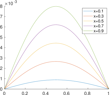
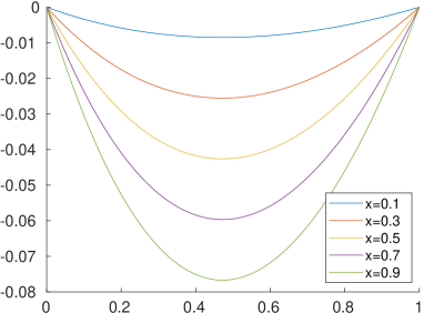
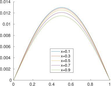
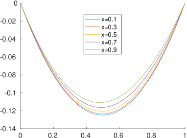
Figure 1: Riesz functions for the system (22): $\eta_{1,i}$ (top-left), $\eta^{\prime\prime}_{1,i}$ (top-right), $\eta_{2,i}$ (bottom-left), and $\eta^{\prime\prime}_{2,i}$ (bottom-right), with $x_{i}=0.1+0.2(i-1)$ for $i=1,\ldots,5$.

Example 6.

Let us consider the system

$$\begin{cases}\displaystyle\int_{0}^{\pi}{\mathrm{e}}^{x\cos{t}}f(t)\,dt=2\frac{\sinh{x}}{x},\\ \displaystyle\int_{0}^{\pi}(xt+{\mathrm{e}}^{xt})f(t)\,dt=\pi x+\frac{1+{\mathrm{e}}^{\pi x}}{1+x^{2}},\end{cases}$$ (27)

with $x\in(0,\pi/2]$, whose exact solution is $f(t)=\sin t$. This system has been obtained by coupling the well-known Baart test problem [24] with another equation having the same solution.

From (21) we have, for $i=1,\ldots,n$,

$$\eta_{2,i}^{\prime\prime}(z)=\frac{z(1-{\mathrm{e}}^{\pi x_{i}})}{\pi x_{i}^{2}}+\frac{x_{i}z(z^{2}-\pi^{2})}{6}+\frac{{\mathrm{e}}^{x_{i}z}-1}{x_{i}^{2}},$$ (28)

and from (20)

$$\eta_{2,i}(y) =\frac{\pi^{2}x_{i}y}{36}\left(\frac{7}{10}\pi^{2}-y^{2}\right)+\frac{y}{6\pi x_{i}^{4}}(1-{\mathrm{e}}^{\pi x_{i}})(x_{i}^{2}y^{2}+6)$$ (29)

$$\phantom{=\ }+\frac{\pi y}{6x_{i}^{2}}({\mathrm{e}}^{\pi x_{i}}+2)+\frac{y^{2}}{2}\left(\frac{x_{i}y^{3}}{60}-\frac{1}{x_{i}^{2}}\right)+\frac{{\mathrm{e}}^{x_{i}y}-1}{x_{i}^{4}}.$$

The functions $\eta_{1,i}^{\prime\prime}(z)$ and $\eta_{1,i}(y)$ do not have an analytic representation, so they should be approximated by a quadrature formula.

Let us now compute the coefficient of the expansion (19) of the minimal-norm solution. By replacing $f$ in (9) by (19), we obtain

$$(K_{\ell}f^{\dagger})(x_{\ell,i})=g_{\ell}(x_{\ell,i}),\qquad\ell=1,\dots,m,\quad i=1,\dots,n_{\ell},$$

namely,

$$\sum_{\ell=1}^{m}\sum_{k=1}^{n_{\ell}}(K_{\ell}\eta_{\ell,k})(x_{\ell,i})c_{k+N_{\ell-1}}=g_{\ell}(x_{\ell,i}),$$

where $\eta_{\ell,k}:=\eta_{k+N_{\ell-1}}$ and the integers $N_{\ell}$ are defined in (16). By renumbering the Riesz representers, we obtain the square linear system

$$\sum_{j=1}^{N_{m}}(K_{\ell}\eta_{j})(x_{\ell,i})c_{j}=g_{\ell}(x_{\ell,i}),\qquad\ell=1,\dots,m,\quad i=1,\dots,n_{\ell}.$$

Taking into account (17), the above linear system can be written in matrix form as

$${\mathcal{G}}\mathbf{c}=\mathbf{g},$$ (30)

where $\mathbf{g}$ is defined in (11) and $\mathbf{c}=[c_{j}]_{j=1}^{N_{m}}$ is the vector of the unknowns. The Gram matrix ${\mathcal{G}}\in\mathbb{R}^{N_{m}\times N_{m}}$ is defined as

$${\mathcal{G}}=\begin{bmatrix}{\mathcal{G}}^{1}&\Gamma^{1,2}&\cdots&\Gamma^{1,m}\\ (\Gamma^{1,2})^{T}&{\mathcal{G}}^{2}&&\vdots\\ \vdots&&\ddots&\vdots\\ (\Gamma^{1,m})^{T}&\cdots&\cdots&{\mathcal{G}}^{m}\end{bmatrix},$$ (31)

where the entries of the $m$ diagonal blocks ${\mathcal{G}}^{\ell}$, $\ell=1,\dots,m$, are

$${\mathcal{G}}^{\ell}_{ij}=\langle\eta_{\ell,i},\eta_{\ell,j}\rangle_{W},$$ (32)

and the off-diagonal blocks $\Gamma^{\ell,k}$, with $\ell,k=1,\dots,m$, $k>\ell$, have entries

$$\Gamma^{\ell,k}_{ij}=\langle\eta_{\ell,i},\eta_{k,j}\rangle_{W},$$ (33)

for $i=1,\dots,n_{\ell}$ and $j=1,\dots,n_{k}$.

The inner products in (32) and (33) involve the second derivatives $\eta_{\ell,i}^{\prime\prime}$. Whenever they can be computed analytically, the elements of the Gram matrix ${\mathcal{G}}$ can be obtained by symbolic computation; we used the integral function of Matlab. If this is not possible, a Gaussian quadrature formula is adopted.

As it is well-known, the Gram matrix ${\mathcal{G}}$ defined in (31) is symmetric positive definite. Then, a natural approach for solving system (30) would be to apply Cholesky factorization. However, as this linear system results from the discretization of an ill-posed problem, the matrix ${\mathcal{G}}$ is severely ill-conditioned. Since experimental data is typically contaminated by noise, the numerical solution of (30) is subject to strong error propagation and can deviate substantially from the exact solution. Moreover, the numerical computation of the Cholesky factorization may lead to computing the square root of small negative quantities, making it impossible to construct the Cholesky factor.

We adopted a different approach, consisting of writing the Gram matrix in terms of its spectral factorization [38]

$${\mathcal{G}}=U\Lambda U^{T},$$ (34)

where the diagonal matrix $\Lambda=\mathop{\operator@font diag}\nolimits(\lambda_{1},\lambda_{2},\dots,\lambda_{N_{m}})$ contains the eigenvalues of ${\mathcal{G}}$ sorted by decreasing value, and $U=[\mathbf{u}_{1},\dots,\mathbf{u}_{N_{m}}]$ is the eigenvector matrix with orthonormal columns.

Then, by employing (34) in system (30), we obtain the following representation for the coefficients

$$\mathbf{c}=[c_{1},\ldots,c_{N_{m}}]^{T}=\sum_{\ell=1}^{N_{m}}\frac{\mathbf{u}_{\ell}^{T}\mathbf{g}}{\lambda_{\ell}}\mathbf{u}_{\ell},$$ (35)

of the minimal-norm solution

$$f^{\dagger}=\sum_{j=1}^{N_{m}}c_{j}\eta_{j},$$ (36)

resulting from Theorem 4.

4 Regularized minimal-norm solution

The severe ill-conditioning of the matrix ${\mathcal{G}}$ produces a strong error propagation in (35) and, consequently, in the solution (36). A regularized solution is needed, instead.

In what follows, it is convenient to write $f^{\dagger}$ as a linear combination of orthonormal functions. The orthonormalization of a family of functions is a classical topic in functional analysis. The properties arising from the orthogonalization of the translates of a given function, and the connections of such process to the factorization of the associated Gram matrix have been investigated in [15, 17], and later generalized to multivariate functions in [18]. A review of the available algorithms for the spectral factorization of infinite Gram matrices is contained in [16].

The following theorem shows how an orthonormal expansion for the minimal-norm solution can be constructed by (34), and gives the expression of such orthonormal functions which are, in fact, the singular functions [12, 29] of the integral operator $\mathbf{K}$.

Theorem 7.

The minimal-norm solution $f^{\dagger}$ of (10) can be written as a linear combination of orthonormal functions $\widehat{\eta}_{\ell}$

$$f^{\dagger}=\sum_{\ell=1}^{N_{m}}\widehat{c}_{\ell}\widehat{\eta}_{\ell},$$ (37)

where

$$\widehat{c}_{\ell}=\frac{\mathbf{u}_{\ell}^{T}\mathbf{g}}{\sqrt{\lambda_{\ell}}},\qquad\widehat{\eta}_{\ell}=\sum_{j=1}^{N_{m}}\frac{u_{j\ell}}{\sqrt{\lambda_{\ell}}}\eta_{j},\qquad\ell=1,\ldots,N_{m},$$ (38)

and $u_{j\ell}$ denotes the $j$th component of the eigenvector $\mathbf{u}_{\ell}$ with eigenvalue $\lambda_{\ell}$ in the spectral factorization (34). Moreover, the set of the triplets $\left\{\sqrt{\lambda_{\ell}},\widehat{\eta}_{\ell},\mathbf{u}_{\ell}\right\}$, $\ell=1,\ldots,N_{m}$, is the singular system of the operator $\mathbf{K}$ (10).

Proof.

Starting from (36) and (35), changing the order of summation, we obtain

$$f^{\dagger}=\sum_{j=1}^{N_{m}}c_{j}\eta_{j}=\sum_{j=1}^{N_{m}}\sum_{\ell=1}^{N_{m}}\frac{\mathbf{u}_{\ell}^{T}\mathbf{g}}{\lambda_{\ell}}u_{j\ell}\eta_{j}=\sum_{\ell=1}^{N_{m}}\frac{\mathbf{u}_{\ell}^{T}\mathbf{g}}{\sqrt{\lambda_{\ell}}}\sum_{j=1}^{N_{m}}\frac{u_{j\ell}}{\sqrt{\lambda_{\ell}}}\eta_{j}.$$

Equation (37) follows by defining $\widehat{c}_{\ell}$ and $\widehat{\eta}_{\ell}$ as in (38).

Let us now prove the final statement of the theorem. It is immediate to verify that the functions $\widehat{\eta}_{\ell}$, $\ell=1,\ldots,N_{m}$, form an orthonormal basis for ${\mathcal{N}}(\mathbf{K})^{\perp}$. Indeed, letting ${\mathcal{G}}_{ij}=\langle\eta_{i},\eta_{j}\rangle_{W}$ be the elements of ${\mathcal{G}}$, we have

$$\langle\widehat{\eta}_{k},\widehat{\eta}_{h}\rangle_{W} =\sum_{i=1}^{N_{m}}\sum_{j=1}^{N_{m}}\frac{u_{ik}}{\sqrt{\lambda_{k}}}\frac{u_{jh}}{\sqrt{\lambda_{h}}}\langle\eta_{i},\eta_{j}\rangle_{W}=\frac{1}{\sqrt{\lambda_{k}\lambda_{h}}}\sum_{i=1}^{N_{m}}u_{ik}\sum_{j=1}^{N_{m}}{\mathcal{G}}_{ij}u_{jh}$$

$$=\frac{1}{\sqrt{\lambda_{k}\lambda_{h}}}(U^{T}{\mathcal{G}}U)_{kh}=\frac{1}{\sqrt{\lambda_{k}\lambda_{h}}}\Lambda_{kh}=\delta_{kh},$$

where $\delta_{kh}$ is the Kronecker delta and, in the last equality, the matrix ${\mathcal{G}}$ is replaced by its spectral decomposition (34). The orthonormality of the vectors $\mathbf{u}_{\ell}$, $\ell=1,\ldots,N_{m}$, immediately follows from factorization (34).

From the definition (17) of the Riesz representers, we can write

$$(\mathbf{K}\widehat{\eta}_{\ell})_{j} =\langle\eta_{j},\widehat{\eta}_{\ell}\rangle_{W}=\sum_{s=1}^{N_{m}}\frac{u_{s\ell}}{\sqrt{\lambda_{\ell}}}\langle\eta_{j},\eta_{s}\rangle_{W}=\sum_{s=1}^{N_{m}}\frac{u_{s\ell}}{\sqrt{\lambda_{\ell}}}{\mathcal{G}}_{js}=\frac{1}{\sqrt{\lambda_{\ell}}}({\mathcal{G}}U)_{j\ell}$$

$$=\frac{1}{\sqrt{\lambda_{\ell}}}(U\Lambda)_{j\ell}=\sqrt{\lambda_{\ell}}\,u_{j\ell},\qquad j=1,\ldots,N_{m},$$

where the spectral factorization (34) of ${\mathcal{G}}$ is employed again. Then, $\mathbf{K}\widehat{\eta}_{\ell}=\sqrt{\lambda_{\ell}}\mathbf{u}_{\ell}$.

Now, let $f\in W$. Then, $f=f_{0}+f_{1}$, with $f_{0}\in{\mathcal{N}}(\mathbf{K})$, $f_{1}\in{\mathcal{N}}(\mathbf{K})^{\perp}$, and

$$f_{1}=\sum_{j=1}^{N_{m}}\alpha_{j}\widehat{\eta}_{j},\qquad\text{with }\alpha_{j}=\langle f_{1},\widehat{\eta}_{j}\rangle_{W}.$$

By the definition (18) of the adjoint operator, we obtain

$$\langle f,\mathbf{K}^{*}\mathbf{u}_{\ell}\rangle_{W} =\langle\mathbf{K}f,\mathbf{u}_{\ell}\rangle_{2}=\langle\mathbf{K}f_{1},\mathbf{u}_{\ell}\rangle_{2}=\sum_{j=1}^{N_{m}}\alpha_{j}\langle\mathbf{K}\widehat{\eta}_{j},\mathbf{u}_{\ell}\rangle_{2}$$

$$=\sum_{j=1}^{N_{m}}\alpha_{j}\left\langle\sqrt{\lambda_{j}}\mathbf{u}_{j},\mathbf{u}_{\ell}\right\rangle_{2}=\alpha_{\ell}\sqrt{\lambda_{\ell}}=\langle f,\sqrt{\lambda_{\ell}}\widehat{\eta}_{\ell}\rangle_{W},$$

since $\alpha_{\ell}=\langle f_{1},\widehat{\eta}_{\ell}\rangle_{W}=\langle f,\widehat{\eta}_{\ell}\rangle_{W}$. Then $\mathbf{K}^{*}\mathbf{u}_{\ell}=\sqrt{\lambda_{\ell}}\widehat{\eta}_{\ell}$. It follows that

$$\mathbf{K}^{*}\mathbf{K}\widehat{\eta}_{\ell}=\lambda_{\ell}\widehat{\eta}_{\ell},\qquad\mathbf{K}\mathbf{K}^{*}\mathbf{u}_{\ell}=\lambda_{\ell}\mathbf{u}_{\ell},\qquad\ell=1,\ldots,N_{m}.$$

This completes the proof. ∎

We remark that Theorem 7 is applicable under the assumption that the Gram matrix ${\mathcal{G}}$ is positive definite. In practice, because of error propagation, the smallest numerical eigenvalues of ${\mathcal{G}}$ may become zero, or even negative. In this case, that is, if $\lambda_{N_{m}}\leq 0$, we replace $N_{m}$ in all summations by an integer $N<N_{m}$ such that $\lambda_{N}>0\geq\lambda_{N+1}$.

From (37) and from the definition of $\widehat{\mathbf{c}}$ in (38), it follows that

$$\|f^{\dagger}\|_{W}=\|\widehat{\mathbf{c}}\|_{2}=\|L\mathbf{c}\|_{2},\qquad\text{with }L=\Lambda^{1/2}U^{T},$$ (39)

where the relation between $\mathbf{c}$ and $\widehat{\mathbf{c}}$ is obtained by (38), writing $\widehat{\mathbf{c}}$ in matrix form

$$\widehat{\mathbf{c}}=\Lambda^{-1/2}U^{T}\mathbf{g}=\Lambda^{-1/2}U^{T}{\mathcal{G}}\mathbf{c}=\Lambda^{-1/2}U^{T}U\Lambda U^{T}\mathbf{c}=\Lambda^{1/2}U^{T}\mathbf{c}.$$

This expression for $\widehat{\mathbf{c}}$ is equivalent to solving the linear system $\widehat{{\mathcal{G}}}\,\widehat{\mathbf{c}}=\mathbf{g}$, whose coefficient matrix $\widehat{{\mathcal{G}}}=U\Lambda^{1/2}$ has a condition number which is the square root of that of ${\mathcal{G}}$.

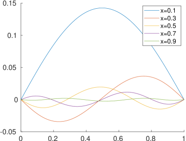
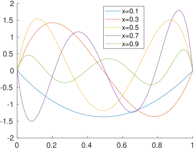
Figure 2: Orthonormalized Riesz functions for the system (22): $\widehat{\eta}_{1,i}$ (top-left) and $\widehat{\eta}^{\prime\prime}_{1,i}$ (top-right) for $x_{i}=0.1+0.2(i-1)$, $i=1,\ldots,5$; $\widehat{\eta}_{2,i}$ (bottom-left) and $\widehat{\eta}^{\prime\prime}_{2,i}$ (bottom-right) are displayed only for $x_{1}$ and $x_{2}$.

In order to handle ill-conditioning, as it is customary, we replace the original problem with a nearby one, whose solution is less sensitive to the error present in the data. The representation (37) is particularly suitable to construct a regularized solution. Indeed, according to the “discrete” Picard condition [23, Section 4.5], the numerators in the coefficients $\widehat{c}_{\ell}$ should decay to zero faster than the denominators. Anyway, the presence of noise in the right-hand side $\mathbf{g}$ will prevent the projections $\mathbf{u}_{\ell}^{T}\mathbf{g}$ from decaying when $\ell$ increases, leading to severe growth in the values of the coefficients. Truncating the summation in (37) removes the noisy components of the solution that are enhanced by ill-conditioning. Moreover, it damps the high frequency components represented by the $\widehat{\eta}_{\ell}$ functions with a large index $\ell$.

The association of high frequencies to small singular values cannot be proved in general. However, in the case of first kind integral equations with a smooth kernel, it has been observed that singular functions associated with the smallest singular values oscillate much, while those corresponding to large singular values are smooth. For example, Figure 2 displays the functions $\widehat{\eta}_{\ell}$ obtained by applying formula (38) to the Riesz functions constructed in Example 5. In the summation (38), the upper bound for the index is fixed at $N=7$, to preserve the positivity of the eigenvalues. The graphs in the left column depict the orthonormal functions, and the ones in the right column their second derivatives. It is immediate to observe the increasing frequency of the orthonormal basis.

The graphs of the functions $\widehat{\eta}_{2,1}$ and $\widehat{\eta}_{2,2}$ in the bottom-left panel of Figure 2 are extremely jagged, showing that there is a strong error propagation in the numerical construction of the orthonormal functions. This deters from employing the orthonormal basis in the real computation, unless a more stable orthonormalization process is implemented. Anyway, as we will show, the functions $\widehat{\eta}_{\ell}$ are only implicitly used in the construction of the regularized solution.

Indeed, the regularized solution is obtained by choosing an index $\kappa$ to truncate the summation in (37), i.e., $1\leq\kappa\leq N$, leading to the expression

$$f^{(\kappa)}=\sum_{\ell=1}^{\kappa}\widehat{c}_{\ell}\widehat{\eta}_{\ell}=\sum_{\ell=1}^{\kappa}\frac{\mathbf{u}_{\ell}^{T}\mathbf{g}}{\sqrt{\lambda_{\ell}}}\sum_{j=1}^{N}\frac{u_{j\ell}}{\sqrt{\lambda_{\ell}}}\eta_{j}=\sum_{j=1}^{N}\sum_{\ell=1}^{\kappa}\frac{\mathbf{u}_{\ell}^{T}\mathbf{g}}{\lambda_{\ell}}u_{j\ell}\eta_{j}=\sum_{j=1}^{N}c^{(\kappa)}_{j}\eta_{j}.$$ (40)

This shows that $f^{(\kappa)}$ can be expressed as a linear combination of the Riesz representers $\eta_{j}$ and there is no need to explicitly construct the singular functions $\widehat{\eta}_{\ell}$.

The coefficients in the last summation correspond to the truncated eigendecomposition (TEIG) solution of system (30) (see [1, 14] for more details) with parameter $\kappa\leq N$, defined to be the components of the vector

$$\mathbf{c}^{(\kappa)}=U\Lambda_{\kappa}^{\dagger}U^{T}\mathbf{g}=\sum_{\ell=1}^{\kappa}\frac{\mathbf{u}_{\ell}^{T}\mathbf{g}}{\lambda_{\ell}}\mathbf{u}_{\ell},$$ (41)

where $\Lambda_{\kappa}^{\dagger}$ denotes the Moore-Penrose pseudoinverse [6] of $\Lambda_{\kappa}=\mathop{\operator@font diag}\nolimits(\lambda_{1},\dots,\lambda_{\kappa},0,\ldots,0)$. We observe that, because of the orthonormality of the functions $\widehat{\eta}_{\ell}$, $\|f^{(\kappa)}\|_{W}\leq\|f^{(\kappa+1)}\|_{W}\leq\|f^{\dagger}\|_{W}$.

It is possible to show that the above vector $\mathbf{c}^{(\kappa)}$ solves the optimization problem

$$\begin{cases}\displaystyle\min_{\mathbf{c}}\|L\mathbf{c}\|_{2}\\ \displaystyle\mathbf{c}\in\bigl{\{}\arg\min_{\mathbf{c}}\|{\mathcal{G}}_{\kappa}\mathbf{c}-\mathbf{g}\|_{2}\bigr{\}},\end{cases}$$

where ${\mathcal{G}}_{\kappa}=U\Lambda_{\kappa}U^{T}$ is the TEIG of ${\mathcal{G}}$. Therefore, from the algebraic point of view, the computation of $f^{(\kappa)}$ corresponds to selecting the minimal-$L$-norm vector among the solutions of the best rank-$\kappa$ approximation of system (30). Equation (39) shows that the regularized solution $f^{(\kappa)}$ has minimal-norm in $W$.

A crucial point in the regularization process, in order to get an accurate solution, is the estimation of the truncation parameter $\kappa$ in (40) and (41). There exist many methods, either a posteriori or heuristic, aiming at this; see [12, 23, 34]. In this paper, we focus our attention on the discrepancy principle and the L-curve method.

We assume that the exact right-hand side vector $\mathbf{g}_{\text{exact}}$ is contaminated by an unknown normally distributed noise vector $\mathbf{e}$, i.e.,

$$\mathbf{g}=\mathbf{g}_{\text{exact}}+\mathbf{e}.$$ (42)

If $\|\mathbf{e}\|_{2}$ is known, we can apply the discrepancy principle [31], which selects the smallest truncation parameter $\kappa_{\text{d}}$ such that

$$\|{\mathcal{G}}\mathbf{c}^{(\kappa_{\text{d}})}-\mathbf{g}\|_{2}\leq\tau\|\mathbf{e}\|_{2},$$ (43)

where $\tau>1$ is a constant independent of the noise level $\|\mathbf{e}\|_{2}$. Note that from (34) and (41), we can write the residual norm as

$$\|{\mathcal{G}}\mathbf{c}^{(\kappa)}-\mathbf{g}\|_{2}^{2}=\|U(\Lambda\Lambda_{\kappa}^{\dagger}-I)U^{T}\mathbf{g}\|_{2}^{2}=\sum_{j=\kappa+1}^{N_{m}}(\mathbf{u}_{j}^{T}\mathbf{g})^{2}.$$ (44)

This relation shows that the residual is non-decreasing when $\kappa$ decreases and it allows reducing the computational load. Indeed, the projected vector $U^{T}\mathbf{g}$ is computed in any case, once the spectral factorization of ${\mathcal{G}}$ is available, since its first $\kappa$ components are required for (41), but the value of $\kappa$ is not a priori known.

When the noise level is unknown, we use the L-curve criterion [22, 26], which selects the regularization parameter $\kappa_{\text{lc}}$ at the “corner” of the curve joining the points

$$\left(\log\|{\mathcal{G}}\mathbf{c}^{(\kappa)}-\mathbf{g}\|_{2},\;\log\|f^{(\kappa)}\|_{W}\right),\qquad\kappa=1,\ldots,N,$$ (45)

where $f^{(\kappa)}$ is the function defined in (40) and

$$\|f^{(\kappa)}\|_{W}=\|L\mathbf{c}^{(\kappa)}\|_{2}=\sqrt{(\mathbf{c}^{(\kappa)})^{T}{\mathcal{G}}\mathbf{c}^{(\kappa)}}.$$

When solving discrete ill-posed problems, this curve often exhibits a typical L-shape. We determine its corner by the method described in [25] and implemented in [24].

When the exact solution $f$ is available, to ascertain the best possible performance of the algorithms independently of the strategy adopted for the estimation of the regularization parameter, in the numerical experiments we also consider the parameter $\kappa_{\text{best}}$ which minimizes the norm of the error, that is,

$$\kappa_{\text{best}}=\arg\min_{\kappa}\|f-f^{(\kappa)}\|_{W}=\arg\min_{\kappa}\|L(\mathbf{c}-\mathbf{c}^{(\kappa)})\|_{2}.$$ (46)

Remark 8.

We observe that the operator ${\mathcal{F}}_{\text{d}}$, which assigns to a noisy right-hand side $\mathbf{g}$ (see (42) and (47)) the regularized solution $f^{(\kappa_{\text{d}})}$ (40) corresponding to the regularization parameter $\kappa_{\text{d}}=\kappa_{\text{d}}(\delta,\mathbf{g})$ estimated by the discrepancy principle, is trivially a regularization method in the sense of [12, Definition 3.1]. Indeed, from (43) and (44), $\kappa_{\text{d}}=N_{m}$ when $\delta\to 0$, and $f^{(N_{m})}$ coincides with the minimal-norm solution $f^{\dagger}$.

5 Numerical tests

In this section, we report some numerical results obtained by applying our algorithm to the two examples presented in Section 3. All the computations were performed on an Intel Xeon E-2244G system with 16Gb RAM, running Matlab 9.10. The software developed is only prototypal, but it is available from the authors upon request.

In each numerical test, we consider the exact right-hand side ${\mathbf{g}}_{\text{exact}}$ of the linear system (30), corresponding to the collocation nodes $x_{\ell,i}$, for $\ell=1,\ldots,m$ and $i=1,\ldots,n_{\ell}$. We add Gaussian noise as in (42), where the noise vector $\mathbf{e}$ is defined by

$$\mathbf{e}=\frac{\delta}{\sqrt{N_{m}}}\|{\mathbf{g}}_{\text{exact}}\|_{2}\mathbf{w},$$ (47)

with $N_{m}$ as in (16). The components of the vector $\mathbf{w}$ are normally distributed with zero average and unit variance, and $\delta$ represents the noise level. For the sake of simplicity, for each system we consider the same collocation nodes $x_{\ell,i}$ in both equations, so that $m=2$, $n_{1}=n_{2}=n$, $N_{m}=2n$, and $x_{1,i}=x_{2,i}$, for $i=1,\dots,n$.

Test problem 1.

We consider the system (22) described in Example 5. It consists of two Fredholm integral equations of the first kind, with $x\in(0,1]$ and exact solution $f(t)=t^{2}+1$. In this example we set $x_{\ell,i}=0.1+0.9\,(i-1)/(n-1)$, for $\ell=1,2$ and $i=1,\ldots,n$.

The corresponding Riesz representers have been computed analytically in (25) and (26). Note that the analytic expression of $\eta^{\prime\prime}_{\ell,i}$ defined in (23) and (24) allows for an accurate computation of the elements of the Gram matrix (31) and for obtaining an explicit representation of the functions $\eta_{\ell,i}$, providing a fast and accurate algorithm.

We remind the reader that, by (7), the solution of this problem is expressed as

$$f(t)=\xi(t)+\gamma(t),$$

where $\gamma(t)=t+1$ is the function (5) and $\xi(t)$ is the solution of the system (6).

To start with, we depict in Figure 3 the non-regularized reconstructions of the solution, obtained for $n=5,10,20$, without noise in the data, and the corresponding error curves with respect to the exact solution. By “non-regularized”, we mean that we set $\kappa=N$ in (40) and (41). The fact that the errors are so small is remarkable. Indeed, setting $\delta=0$ in (47) only guarantees that the right-hand side is accurate up to machine precision, that is, roughly $10^{-16}$. Since the estimation of the condition number of the Gram matrix ${\mathcal{G}}$ provided by the cond function of Matlab for the three problem sizes considered is $2.2\cdot 10^{18}$, $6.9\cdot 10^{32}$, and $1.1\cdot 10^{19}$, respectively, the results highlight the stability in the computation, as well as the effectiveness of the function space setting.

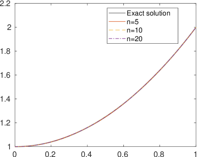
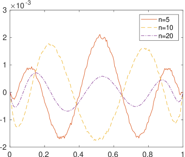
Figure 3: Non-regularized reconstructions of the solution of Test problem 1 (left) and corresponding errors (right), for $n=5,10,20$, and without noise.

Figure 4 shows, in the left pane, the reconstructions obtained without regularization for $n=5,10,20$, together with the exact solution, when the data vector is affected by noise with level $\delta=10^{-4}$. Due to the large condition number, the computed solutions are polluted by noise propagation to such a point that they oscillate at high frequency away from the exact solution. The graph on the right of the same figure displays the results obtained by computing the regularized solution $f^{(\kappa)}$ defined in (40). Here, the truncation parameter $\kappa$ coincides with the value $\kappa_{\text{best}}$, defined in (46), corresponding to the best possible performance of the algorithm. The quality of the results is excellent.

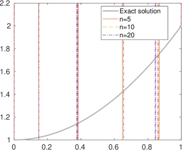
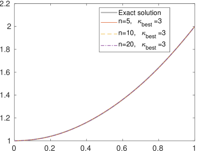
Figure 4: On the left: non-regularized solutions of Test problem 1, for $n=5,10,20$, and noise level $\delta=10^{-4}$. On the right: regularized solution $f^{(\kappa_{\text{best}})}(t)$, for $n=5,10,20$, and $\delta=10^{-4}$; the optimal value $\kappa_{\text{best}}$ of the regularization parameter is displayed in the legend.

The graph on the left of Figure 5 investigates the sensitivity of the solution to the noise level. It shows the errors obtained for $n=10$ and $\delta=10^{-8},10^{-4},10^{-2}$. The graph confirms the accuracy and stability of the proposed regularization method. In the graph on the right, we compare the “best” solution for the noise level $\delta=10^{-4}$ to the ones obtained by estimating the regularization parameter $\kappa_{\text{d}}$ by the discrepancy principle (43), with $\tau=1.1$, and by the L-curve criterion (45), where the truncation parameter $\kappa_{\text{lc}}$ is detected by the algorithm described in [25]. Both estimation techniques are successful.

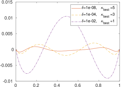
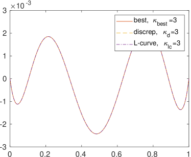
Figure 5: On the left: errors corresponding to the regularized solutions $f^{(\kappa_{\text{best}})}(t)$ of Test problem 1, for $n=10$ and $\delta=10^{-8},10^{-4},10^{-2}$. On the right: errors for the solutions $f^{(\kappa)}(t)$, for $n=20$, $\delta=10^{-4}$, and different estimation methods for $\kappa$. The values of the regularization parameters $\kappa_{\text{best}}$, $\kappa_{\text{d}}$, and $\kappa_{\text{lc}}$ are displayed in the legend.

Test problem 2.

Let us now consider the system (27) introduced in Example 6, with $x\in(0,\pi/2]$. It pairs the well-known Baart test problem [24] to an equation having the same solution $f(t)=\sin t$. The collocation points are $x_{\ell,i}=0.1+(\pi/2-0.1)\,(i-1)/(n-1)$, for $\ell=1,2$ and $i=1,\ldots,n$.

In this example, we were only able to analytically compute the Riesz representers for the second equation; see (28) and (29). An approximation of the Riesz representers for the first equation was computed by a Gauss-Legendre quadrature formula.

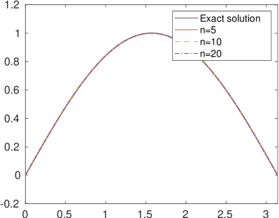
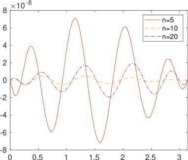
Figure 6: Non-regularized reconstructions of the solution of Test problem 2 (left) and corresponding errors (right), for $n=5,10,20$ and without noise.

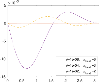
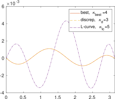
Figure 7: On the left: errors corresponding to the regularized solutions $f^{(\kappa_{\text{best}})}(t)$ of Test problem 2, for $n=10$ and $\delta=10^{-8},10^{-4},10^{-2}$. On the right: errors for the solutions $f^{(\kappa)}(t)$, for $n=20$, $\delta=10^{-4}$, and different estimation methods for $\kappa$. The values of the regularization parameters $\kappa_{\text{best}}$, $\kappa_{\text{d}}$, and $\kappa_{\text{lc}}$ are displayed in the legend.

Figure 6 shows that, when the data vector is only affected by rounding errors, the non-regularized solution is very accurate. On the contrary, as in the previous example, the non-regularized solution is strongly unstable when a sensible amount of noise is added to the data; we do not display the results for the sake of brevity.

The graph on the left of Figure 7 depicts the behavior of the best regularized solutions corresponding to the three noise levels $\delta=10^{-8},10^{-4},10^{-2}$. All the reconstructions are accurate. In the second graph, we compare the error corresponding to the optimal regularization parameter to the ones produced by the discrepancy principle and the L-curve. Even if the estimated values of the parameter are slightly different, the results are satisfactory. We verified that the outcome is not sensibly influenced by the size of the problem.

A discretization of the Baart integral equation [4] is implemented in the Regularization Tools library by P. C. Hansen [24]. The routine baart adopts a Galerkin discretization based on orthonormal box functions. We implemented the same discretization method for the second equation of (27), in order to compare this approach with the one we propose.

Table 1 shows the results obtained by the Galerkin approach compared to the method described in this paper; no regularization method is applied for the solution of the corresponding linear systems and the right-hand sides are exact up to machine precision. The numbers reported in the table represent the infinity norm errors between the exact and the approximate solutions computed on a discretization of the interval $[0,\pi]$. It is clear that there is a strong propagation of rounding errors for the first method, while the solutions computed by the Riesz approach are very accurate (see also Figure 6) thanks to the choice of the function spaces and to the effective use of the boundary information on the solution.

Table 1: Infinity norm errors obtained by discretizing Test problem 2 by a Galerkin method (see the function baart in [24]) and the proposed approach based on Riesz theory; the data is free from noise and no regularization is applied.

$n$	Galerkin	Riesz
6	$3.12\cdot 10^{-1}$	$7.44\cdot 10^{-9}$
10	$8.78\cdot 10^{-1}$	$5.16\cdot 10^{-9}$
20	$4.38\cdot 10^{4\phantom{-}}$	$1.94\cdot 10^{-8}$

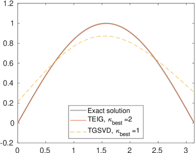
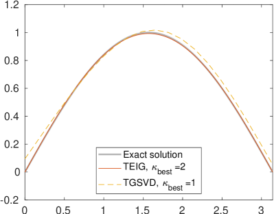
Figure 8: Regularized solutions $f^{(\kappa_{\text{best}})}(t)$ of Test problem 2, for $n=20$ and $\delta=10^{-2}$, obtained by applying TGSVD to the linear system resulting from the Galerkin discretization, and by the new proposed method, labelled as TEIG. On the left, we report the two solutions for the first equation of system (27), on the right the solutions of the system. The values of the optimal regularization parameters $\kappa_{\text{best}}$ are displayed in the legend.

We performed a similar comparison in the presence of noise in the data, setting $\delta=10^{-2}$ in (47), and solving Test problem 2 for $n=20$. In Figure 8, the Galerkin approach is regularized by the truncated generalized singular value decomposition (TGSVD) [23] with a discrete approximation of the second derivative operator as a regularization matrix. The obtained solution is compared to the one produced by the method described in Section 4.

The graph on the left reports the results for the first equation of system (27), while the one on the right corresponds to the complete system. It is evident that the new method is more accurate than the Galerkin/TGSVD approach. At the same time, the graphs also show that there is some advantage in solving the system rather than a single equation. There is a slight improvement in the error also for the Riesz approach, but this is not visible in the graph since the order of the infinity norm error is $10^{-2}$.

6 A case study

Let us consider the following system of integral equations of the first kind

$$\begin{cases}\displaystyle\int_{0}^{\infty}k^{V}(z+h)\sigma(z)\,dz=g^{V}(h),\qquad h\in[0,\infty),\\ \displaystyle\int_{0}^{\infty}k^{H}(z+h)\sigma(z)\,dz=g^{H}(h),\qquad h\in[0,\infty),\end{cases}$$ (48)

proposed in [30] for reproducing the readings of a ground conductivity meter, a frequency domain electromagnetic (FDEM) induction device; see Section 1. In the above equations,

$$k^{V}(z)=\dfrac{4z}{(4z^{2}+1)^{3/2}},\qquad k^{H}(z)=2-\dfrac{4z}{(4z^{2}+1)^{1/2}}$$ (49)

are the kernel functions corresponding to the vertical and horizontal orientation of the coils, respectively, $\sigma(z)\geq 0$ is the unknown function that represents the electrical conductivity of the subsoil at depth $z$ below the ground surface, and $g^{V}(h)$, $g^{H}(h)$ are given right-hand sides that represent the apparent conductivity sensed by the device at height $h$ over the ground for the vertical and the horizontal orientation of the coils, respectively. The depth $z$ and the height $h$ are measured in meters, the electrical conductivity in Siemens per meter.

The conditions for the existence and uniqueness of the solution of system (48) have been studied in [11], where three collocation methods were also proposed and compared. In [10], a preliminary version of the method presented in this paper was applied to the first equation of the model. Here, we extend the investigation to both equations.

Following [11], assuming the a priori information $\sigma(z)\leq\beta$, for $z>z_{0}$, we split each integral into the sum

$$\int_{0}^{\infty}k_{\ell}(h,z)\sigma(z)\,dz=\int_{0}^{z_{0}}k_{\ell}(h,z)\sigma(z)\,dz+\int_{z_{0}}^{\infty}k_{\ell}(h,z)\sigma(z)\,dz,\qquad\ell=1,2,$$

where $k_{1}(h,z)=k^{V}(h+z)$ and $k_{2}(h,z)=k^{H}(h+z)$.

Given the expression (49) of the kernels, setting $\sigma(z)\simeq\beta$, for $z>z_{0}$ and $z_{0}$ sufficiently large, the last integral can be analytically computed. Then, the system becomes

$$\int_{0}^{z_{0}}k_{\ell}(h,z)\sigma(z)\,dz=g_{\ell}(h)-\beta\int_{z_{0}}^{\infty}k_{\ell}(h,z)\,dz,\qquad\ell=1,2,$$

with $g_{1}(h)=g^{V}(h)$ and $g_{2}(h)=g^{H}(h)$. In this way, system (48) is replaced by

$$\begin{cases}\displaystyle(K_{1}\sigma)(h):=\displaystyle\int_{0}^{z_{0}}k_{1}(h,z)\sigma(z)\,dz=g_{1}(h)-\dfrac{\beta}{\theta(z_{0},h)},\\ \displaystyle(K_{2}\sigma)(h):=\displaystyle\int_{0}^{z_{0}}k_{2}(h,z)\sigma(z)\,dz=g_{2}(h)-\beta\left(\theta(z_{0},h)-2(h+z_{0})\right),\end{cases}$$ (50)

where (see [11])

$$\theta(z,h)=\sqrt{4(z+h)^{2}+1}.$$ (51)

We remark that $(-\theta(z,h))^{-1}$ is a primitive function of $k_{1}(h,z)$, and $2z-\theta(z,h)$ is that of $k_{2}(h,z)$.

To determine a solution by applying the theory developed in Sections 2 and 3, it is necessary to introduce the linear function (5)

$$\gamma(z)=\left(1-\frac{z}{z_{0}}\right)\alpha+\frac{z}{z_{0}}\beta,$$

and assume that the values of the electrical conductivity at the endpoints of the integration interval are known, e.g., $\sigma(0)=\alpha$ and $\sigma(z_{0})=\beta$. The boundary values can usually be approximated in applications; see [11].

By collocating equations (50) at the points $h_{i}$, assuming $n_{1}=n_{2}=n$ and $h_{1,i}=h_{2,i}=h_{i}$, for $i=1,\ldots,n$, we obtain

$$\begin{cases}\displaystyle\int_{0}^{z_{0}}k_{1}(h_{i},z)\phi(z)\,dz=\psi_{1}(h_{i}),\quad i=1,\dots,n,\\ \displaystyle\int_{0}^{z_{0}}k_{2}(h_{i},z)\phi(z)\,dz=\psi_{2}(h_{i}),\quad i=1,\dots,n,\end{cases}$$

where

$$\phi(z)=\sigma(z)-\gamma(z)$$

is the new unknown function, and

$$\psi_{1}(h_{i}) =g_{1}(h_{i})-\frac{\beta}{\theta(z_{0},h_{i})}-\int_{0}^{z_{0}}k_{1}(h_{i},z)\gamma(z)\,dz$$

$$=g_{1}(h_{i})-\frac{\alpha}{\theta(0,h_{i})}-\frac{\alpha-\beta}{2z_{0}}\bigl{[}\operatorname{arcsinh}(2h_{i})-\operatorname{arcsinh}(2(z_{0}+h_{i}))\bigr{]},$$

$$\psi_{2}(h_{i}) =g_{2}(h_{i})-\beta\left(\theta(z_{0},h_{i})-2(h_{i}+z_{0})\right)-\int_{0}^{z_{0}}k_{2}(h_{i},z)\gamma(z)\,dz$$

$$=g_{2}(h_{i})-\left[\frac{(\alpha-\beta)h_{i}}{2z_{0}}+\alpha\right]\theta(0,h_{i})+\frac{\alpha-\beta}{2}\left[\frac{h_{i}}{z_{0}}+1\right]\theta(z_{0},h_{i})$$

$$\phantom{=\ }+2\beta h_{i}-z_{0}(\alpha-\beta)-\frac{a-b}{4z_{0}}\left[\operatorname{arcsinh}(2h_{i})-\operatorname{arcsinh}(2(z_{0}+h_{i}))\right]$$

are the new right-hand sides.

The second derivative of the Riesz representers can be computed analytically. Indeed, from (21), it follows that

$$\eta_{1,i}^{\prime\prime}(x) =\int_{0}^{z_{0}}G^{\prime\prime}_{z}(x)k_{1}(h_{i},z)\,dz$$

$$=\frac{1}{2}\left[\left(1-\frac{x}{z_{0}}\right)\operatorname{arcsinh}(2h_{i})-\operatorname{arcsinh}(2(x+h_{i}))\right.$$

$$\phantom{XXX}\left.+\frac{x}{z_{0}}\operatorname{arcsinh}(2(z_{0}+h_{i}))\right]$$

and

$$\eta_{2,i}^{\prime\prime}(x) =\int_{0}^{z_{0}}G^{\prime\prime}_{z}(x)k_{2}(h_{i},z)\,dz$$

$$=\frac{1}{2}\left[2x(x-z_{0})+x\left(1+\frac{h_{i}}{z_{0}}\right)\theta(z_{0},h_{i})-(x+h_{i})\theta(x,h_{i})\right.$$

$$\phantom{XXX}\left.+h_{i}\left(1-\frac{x}{z_{0}}\right)\theta(0,h_{i})+\eta_{1,i}^{\prime\prime}(x)\right],$$

where $\theta(x,h)$ is the function defined in (51). From the above second derivatives, we can compute the Riesz functions

$$\eta_{1,i}(y) =\int_{0}^{z_{0}}G^{\prime\prime}_{y}(x)\eta_{1,i}^{\prime\prime}(x)\,dx$$

$$=\frac{3}{16}\biggl{[}(y+h_{i})\theta(y,h_{i})-y\left(1+\frac{h_{i}}{z_{0}}\right)\theta(z_{0},h_{i})+h_{i}\left(\frac{y}{z_{0}}-1\right)\theta(0,h_{i})\biggr{]}$$

$$\phantom{=}+\frac{1}{2}\left\{\biggl{[}\frac{1}{2}\left(\frac{y}{z_{0}}-1\right)\left(\frac{1}{8}-h_{i}^{2}-\frac{y^{2}}{3}\right)\right.+\frac{y}{3}(y-z_{0})\biggr{]}\operatorname{arcsinh}(2h_{i})$$

$$\phantom{=}+\biggl{[}-\frac{y}{2z_{0}}\left(\frac{1}{8}-h_{i}^{2}-\frac{y^{2}}{3}\right)+y\left(h_{i}+\frac{z_{0}}{3}\right)\biggr{]}\operatorname{arcsinh}(2(z_{0}+h_{i}))$$

$$\phantom{=}\left.+\frac{1}{2}\left[\frac{1}{8}-(y+h_{i})^{2}\right]\operatorname{arcsinh}(2(y+h_{i}))\right\}$$

and

$$\eta_{2,i}(y) =\int_{0}^{z_{0}}G^{\prime\prime}_{y}(x)\eta_{2,i}^{\prime\prime}(x)\,dx$$

$$=\frac{1}{192z_{0}}\Bigl{\{}z_{0}\left[h_{i}\left(13-8(3h_{i}y+h_{i}^{2}+3y^{2})\right)+y(13-8y^{2})\right]\theta(y,h_{i})\Bigl{.}$$

$$\phantom{=}\left.+y\left[h_{i}\left(8(3h_{i}z_{0}+h_{i}^{2}+2y^{2}+z_{0}^{2})-13\right)+z_{0}\left(8(2y^{2}-z_{0}^{2})-13\right)\right]\theta(z_{0},h_{i})\right.$$

$$\phantom{=}\left.+h_{i}\left[z_{0}\left(8(h_{i}^{2}+6y^{2}-4yz_{0})-13\right)+y\left(13-8(h_{i}^{2}+2y^{2})\right)\right]\theta(0,h_{i})\right.$$

$$\phantom{=}\Bigr{.}+16yz_{0}\left(y^{3}-2y^{2}z_{0}+z_{0}^{3}\right)\Bigr{\}}$$

$$\phantom{=}+\frac{1}{128z_{0}}\left\{\left(y-z_{0}\right)\left[1-16\left(h_{i}^{2}+\frac{y^{2}}{3}-\frac{2yz_{0}}{3}\right)\right]\operatorname{arcsinh}(2h_{i})\right.$$

$$\phantom{=}\left.+z_{0}\left[1-16\left(y+h_{i}\right)^{2}\right]\operatorname{arcsinh}(2(y+h_{i})\right.$$

$$\phantom{=}\left.-y\left[1-16\left(h_{i}^{2}+\frac{y^{2}}{3}+2h_{i}z_{0}+\frac{2z_{0}^{2}}{3}\right)\right]\operatorname{arcsinh}(2(z_{0}+h_{i}))\right\}.$$

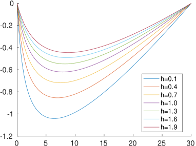
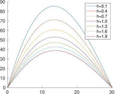
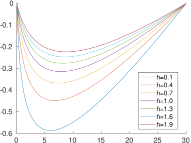
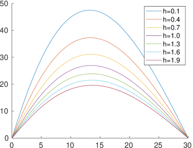
Figure 9: The functions $\eta_{1,i}^{\prime\prime}$ (top-left), $\eta_{1,i}$ (top-right), $\eta_{2,i}^{\prime\prime}$ (bottom-left), and $\eta_{2,i}$ (bottom-right), with $h_{i}=0.1+(i-1)\frac{3}{10}$ and $i=1,\ldots,7$.

Figure 9 shows the behavior of $\eta_{1,i}^{\prime\prime}$ and $\eta_{1,i}$ for different values of $h_{i}$, in the case $z_{0}=30$. We also report the graphs of the Riesz representers for the horizontal orientation $\eta_{2,i}^{\prime\prime}$ and $\eta_{2,i}$. Figure 10 displays the orthonormal functions $\widehat{\eta}_{1,i}$ and $\widehat{\eta}_{2,i}$ defined in (38), together with their second derivatives $\widehat{\eta}_{1,i}^{\prime\prime}$ and $\widehat{\eta}_{2,i}^{\prime\prime}$. In the summation (38), the upper bound is set to $N=12$ for preserving the positivity of the eigenvalues.

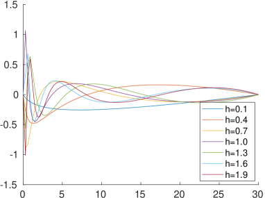
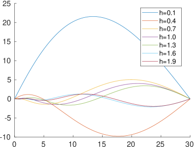
Figure 10: The orthonormal functions $\widehat{\eta}_{1,i}^{\prime\prime}$ (top-left), $\widehat{\eta}_{1,i}$ (top-right), $\widehat{\eta}_{2,i}^{\prime\prime}$ (bottom-left), and $\widehat{\eta}_{2,i}$ (bottom-right), with $h_{i}=0.1+(i-1)\frac{3}{10}$ and $i=1,\ldots,7$.

In order to ascertain the accuracy of our method, when applied to the case study presented in this section, we consider three different profiles for the electrical conductivity $\sigma(z)$. Then, for each test function, we compute the data vector $\boldsymbol{\psi}_{\text{exact}}$, setting $z_{0}=4$ and $h_{i}=0.1+0.9\,(i-1)/(n-1)$, $i=1,\dots,n$, for a chosen dimension $n$.

The computation of the exact data vector is performed by the quadgk function of Matlab, which implements an adaptive Gauss-Kronrod quadrature formula.

In applications, the available data is typically contaminated by errors. The perturbed data vector $\boldsymbol{\psi}$ is determined by adding to $\boldsymbol{\psi}_{\text{exact}}$ a noise-vector $\mathbf{e}$, obtained by substituting in (47) $\boldsymbol{\psi}_{\text{exact}}$ to $\mathbf{g}_{\text{exact}}$ and setting $N_{m}=2n$. The noise level is determined by the parameter $\delta$.

Test function 1.

In the first example, we assume a smooth profile for the exact solution of (48)

$$\sigma_{1}(z)={\mathrm{e}}^{-(z-1)^{2}}+1.$$

We set $\alpha=\sigma_{1}(0)={\mathrm{e}}^{-1}+1$ and $\beta=\sigma_{1}(z_{0})={\mathrm{e}}^{-9}+1$.

We remark that this test function is extremely smooth, so the function $\phi_{1}(z)=\sigma_{1}(z)-\gamma_{1}(z)$ can be assumed to approximately belong to ${\mathcal{N}}(\mathbf{K})^{\perp}=\operatorname{span}\{\eta_{1},\dots,\eta_{N_{m}}\}$, the space which contains the minimal-norm solution.

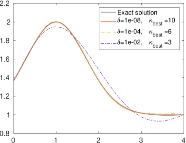
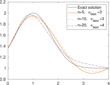
Figure 11: On the left: regularized solution $\sigma_{1}^{(\kappa_{\text{best}})}(z)$ for noise levels $\delta=10^{-8},10^{-4},10^{-2}$, and $n=10$. On the right: regularized solution $\sigma_{1}^{(\kappa_{\text{best}})}(z)$ for $n=5,10,20$, and noise level $\delta=10^{-2}$; the optimal regularization parameter $\kappa_{\text{best}}$ is displayed in the legend.

Figure 11 displays the results obtained by applying the method described in this paper to the electromagnetic integral model (48) with the optimal regularization parameter. On the left-hand side, we report the approximation of the solution for different noise levels $\delta=10^{-8},10^{-4},10^{-2}$, and $n=10$; on the right-hand side, the results for $n=5,10,20$ and $\delta=10^{-2}$ are depicted. All the reconstructions are accurate and identify with sufficient accuracy the maximum value of the conductivity and its depth localization. The graph on the left shows that, even for an increasing noise level, the method is still able to produce reliable results. On the other hand, from the graph on the right we deduce that both the reconstructions and the optimal value of the regularization parameter are not very sensitive on the size of the data vector.

In order to test the method in realistic conditions, in Figure 12 we compare the optimal solution to the approximate solutions corresponding to the parameters $\kappa_{\text{d}}$ and $\kappa_{\text{lc}}$, estimated by the discrepancy principle with $\tau=1.3$ and by the L-curve criterion, respectively. In this case, we have fixed $n=10$ and a noise level $\delta=10^{-4}$. Both estimation techniques appear to be effective.

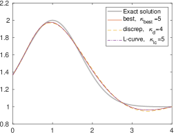
Figure 12: Regularized solution $\sigma_{1}^{(\kappa)}(z)$ with $n=10$ and $\delta=10^{-4}$; the optimal regularization parameter $\kappa_{\text{best}}$ is compared to those determined by the discrepancy principle $\kappa_{\text{d}}$ and by the L-curve $\kappa_{\text{lc}}$.

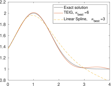
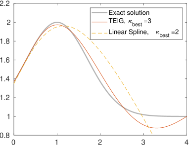
Figure 13: Regularized solutions $\sigma_{1}^{(\kappa_{\text{best}})}(z)$ for $n=20$ by using an approach presented in [11] and the new proposed method. On the left noise level $\delta=10^{-4}$, on the right $\delta=10^{-2}$. The values of the regularization parameters $\kappa_{\text{best}}$ are displayed in the legend.

As already remarked, the linear model (48) has been analyzed in [11], where some collocation methods were discussed. In Figure 13 we compare the most effective technique presented in [11], based on a linear spline approximation coupled to a TGSVD regularization of the resulting linear system, to our new approach. The two graphs report the solutions obtained with two different noise levels, $\delta=10^{-4}$ and $\delta=10^{-2}$, when $n=20$ and choosing the “best” regularization parameter. In both cases, the new method produces more accurate solutions than the linear spline approach. In particular, in the graph on the left, the spline solution is not able to recognize the flattening of the conductivity below 3m depth. In the one on the right, it does not even identify the correct depth of the maximum.

Test function 2.

In the second experiment, we select the following model function

$$\sigma_{2}(z)=\begin{cases}0.8z+0.2,&z\in[0,1],\\ 0.8{\mathrm{e}}^{-(z-1)}+0.2,&z\in(1,\infty),\end{cases}$$

and set $\alpha=0.2$ and $\beta=0.2+0.8{\mathrm{e}}^{-3}$.

The graph in the left pane of Figure 14 reports the optimal regularized solutions corresponding to the noise levels $\delta=10^{-8}$, $10^{-4}$, $10^{-2}$, and $n=10$. The optimal parameter is displayed in the legend. The reconstruction is not accurate as in the previous test, because the solution is non-differentiable and, consequently, it does not belong to ${\mathcal{N}}(\mathbf{K})^{\perp}$. Anyway, the algorithm correctly identifies the position of the maximum of the electrical conductivity at 1m depth.

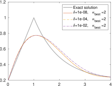
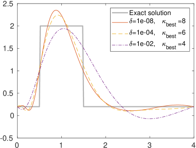
Figure 14: Regularized solution $\sigma_{2}^{(\kappa_{\text{best}})}(z)$ (left) and $\sigma_{3}^{(\kappa_{\text{best}})}(z)$ (right), for $n=10$ and different noise levels $\delta=10^{-8},10^{-4},10^{-2}$; the optimal regularization parameter $\kappa_{\text{best}}$ is displayed in the legend.

Test function 3.

The third model function is the step function

$$\sigma_{3}(z)=\begin{cases}0.2,&z\in(0,0.5),\\ 2,&z\in[0.5,1.5],\\ 0.2,&z\in(1.5,\infty),\end{cases}$$

with $\alpha=\beta=0.2$.

The graph on the right-hand side of Figure 14 reports the optimal regularized solutions for $\delta=10^{-8}$, $10^{-4}$, $10^{-2}$, and $n=10$. Since the function is discontinuous, comments similar to the previous example are valid.

References

- [1] A. Alqahtani, S. Gazzola, L. Reichel, and G. Rodriguez, On the block Lanczos and block Golub-Kahan reduction methods applied to discrete ill-posed problems, Numer. Linear Algebra Appl., 2021 (2021), p. e2376.
- [2] N. Aronszajn, Theory of reproducing kernels, Trans. Am. Math. Soc., 68 (1950), pp. 337–404.
- [3] K. E. Atkinson, The Numerical Solution of Integral Equations of the Second Kind, vol. 552, Cambridge University Press, Cambridge, 1997.
- [4] M. L. Baart, The use of auto-correlation for pseudo-rank determination in noisy ill-conditioned linear least-squares problems, IMA J. Numer. Anal., 2 (1982), pp. 241–247.
- [5] A. Berlinet and C. Thomas-Agnan, Reproducing kernel Hilbert spaces in probability and statistics, Springer, New York, 2004.
- [6] Å. Björck, Numerical Methods for Least Squares Problems, SIAM, Philadelphia, 1996.
- [7] L. P. Castro, H. Itou, and S. Saitoh, Numerical solutions of linear singular integral equations by means of Tikhonov regularization and reproducing kernels, Houston J. Math, 38 (2012), pp. 1261–1276.
- [8] F. Cucker and S. Smale, On the mathematical foundations of learning, Bull. Amer. Math. Soc., 39 (2002), pp. 1–49.
- [9] M. Cui and Y. Lin, Nonlinear Numerical Analysis in the Reproducing Kernel Space, Nova Science Publishers, New York, 2008.
- [10] P. Díaz de Alba, L. Fermo, F. Pes, and G. Rodriguez, Minimal-norm RKHS solution of an integral model in geo-electromagnetism, in 2021 21st International Conference on Computational Science and Its Applications (ICCSA), pp. 21–28.
- [11] P. Díaz de Alba, L. Fermo, C. van der Mee, and G. Rodriguez, Recovering the electrical conductivity of the soil via a linear integral model, J. Comput. Appl. Math., 352 (2019), pp. 132–145.
- [12] H. W. Engl, M. Hanke, and A. Neubauer, Regularization of Inverse Problems, Kluwer, Dordrecht, 1996.
- [13] T. Evgeniou, M. Pontil, and T. Poggio, Regularization networks and support vector machines, Adv. Comp. Math., 13 (2000), pp. 1–50.
- [14] S. Gazzola, E. Onunwor, L. Reichel, and G. Rodriguez, On the Lanczos and Golub–Kahan reduction methods applied to discrete ill-posed problems, Numer. Linear Algebra Appl., 23 (2016), pp. 187–204.
- [15] T. Goodman, C. Micchelli, G. Rodriguez, and S. Seatzu, On the Cholesky factorization of the Gram matrix of locally supported functions, BIT, 35 (1995), pp. 233–257.
- [16] , Spectral factorization of Laurent polynomials, Adv. Comput. Math., 7 (1997), pp. 429–454.
- [17] , On the limiting profile arising from orthonormalizing shifts of exponentially decaying functions, IMA J. Numer. Anal., 18 (1998), pp. 331–354.
- [18] , On the Cholesky factorisation of the Gram matrix of multivariate functions, SIAM J. Matrix Anal. Appl., 22 (2000), pp. 501–526.
- [19] C. W. Groetsch, Elements of Applicable Functional Analysis, vol. 55 of Monographs and Textbooks in Pure and Applied Mathematics, Dekker, New York and Basel, 1980.
- [20] , Integral equations of the first kind, inverse problems and regularization: A crash course, in Journal of Physics: Conference Series, vol. 73, 2007, p. 012001.
- [21] J. Hadamard, Lectures on Cauchy’s Problem in Linear Partial Differential Equations, Yale University Press, New Haven, 1923.
- [22] P. C. Hansen, Analysis of the discrete ill-posed problems by means of the L-curve, SIAM Rev., 34 (1992), pp. 561–580.
- [23] , Rank–Deficient and Discrete Ill–Posed Problems, SIAM, Philadelphia, 1998.
- [24] , Regularization Tools: version 4.0 for Matlab 7.3, Numer. Algorithms, 46 (2007), pp. 189–194.
- [25] P. C. Hansen, T. K. Jensen, and G. Rodriguez, An adaptive pruning algorithm for the discrete L-curve criterion, J. Comput. Appl. Math., 198 (2007), pp. 483–492.
- [26] P. C. Hansen and D. P. O’Leary, The use of the L-curve in the regularization of discrete ill–posed problems, SIAM J. Sci. Comput., 14 (1993), pp. 1487–1503.
- [27] J. M. H. Hendrickx, B. Borchers, D. L. Corwin, S. M. Lesch, A. C. Hilgendorf, and J. Schlue, Inversion of soil conductivity profiles from electromagnetic induction measurements, Soil Sci. Soc. Am. J., 66 (2002), pp. 673–685. Package NONLINEM38 available at http://infohost.nmt.edu/~borchers/nonlinem38.html.
- [28] E. Hille, Introduction to general theory of reproducing kernels, Rocky Mt. J. Math., 2 (1972), pp. 321–368.
- [29] R. Kress, Linear Integral Equation, Springer, Berlin, 1999.
- [30] J. D. McNeill, Electromagnetic terrain conductivity measurement at low induction numbers, Tech. Rep. TN-6, Geonics Limited, Mississauga, Ontario, Canada, 1980.
- [31] V. A. Morozov, The choice of parameter when solving functional equations by regularization, Dokl. Akad. Nauk. SSSR, 175 (1962), pp. 1225–1228.
- [32] F. Pes and G. Rodriguez, The minimal-norm Gauss-Newton method and some of its regularized variants, Electron. Trans. Numer. Anal., 53 (2020), pp. 459–480.
- [33] , A doubly relaxed minimal-norm Gauss–Newton method for underdetermined nonlinear least-squares problems, Appl. Numer. Math., 171 (2022), pp. 233–248.
- [34] L. Reichel and G. Rodriguez, Old and new parameter choice rules for discrete ill-posed problems, Numer. Algorithms, 63 (2013), pp. 65–87.
- [35] G. Rodriguez and S. Seatzu, Numerical solution of the finite moment problem in a reproducing kernel Hilbert space, J. Comput. Appl. Math., 33 (1990), pp. 233–244.
- [36] , On the numerical inversion of the Laplace transform in reproducing kernel Hilbert spaces, IMA J. Numer. Anal., 13 (1993), pp. 463–475.
- [37] Y. Sawano, H. Fujiwara, and S. Saitoh, Real inversion formulas of the Laplace transform on weighted function spaces, Complex Anal. Oper. Theory, 2 (2008), pp. 511–521.
- [38] G. Stewart, Matrix Algorithms: Volume 1: Basic Decompositions, SIAM, Philadelphia, PA, 1998.
- [39] J. Stoer and R. Bulirsch, Introduction to Numerical Analysis, vol. 12 of Texts in Applied Mathematics, Springer-Verlag, New York, second ed., 1991.
- [40] G. Wahba, An introduction to reproducing kernel Hilbert spaces and why they are so useful, in Proceedings of the 13th IFAC Symposium on System Identification (SYSID 2003), 2003.
- [41] R. Wang and Y. Xu, Functional reproducing kernel Hilbert spaces for non-point-evaluation functional data, Appl. Comput. Harmon. Anal., 46 (2019), pp. 569–623.
- [42] , Regularization in a functional reproducing kernel Hilbert space, J. Complex., (2021), p. 101567.
- [43] G. M. Wing, A primer on integral equations of the first kind: the problem of deconvolution and unfolding, SIAM, Philadelphia, PA, 1991.
- [44] K. Yosida, Functional Analysis, Classics in Mathematics, Springer, Berlin, 1995.