1 How to think about LDF

LDF is a model averaging/selection method which provides an estimator for the expected score conditional on the past. It extends the well-established methods using discount factors presented in the literature so far and is not tied to using log scores but generalises to any scoring functions such as focused prediction scores.

We use the notation $\mathcal{D}_{t}$ to denote information available at time $t$, we have $m$ models $M$ and $n$ $\alphas$ are discreet values on a grid between $[0,1]$ and all models use log scores. LDF encapsulates and generalises a few ideas from literature.

• DMA raftery2010online - model averaging with a single discount factor

  $$p(M_{1:m}|\mathcal{D}_{t})\propto p(M_{1:m}|\mathcal{D}_{t-1})^{\alpha}p(y_{t}|\mathcal{D}_{t-1},M_{1:m}),$$

  then use softmax.

• zhao2016dynamic - model averaging single discount factor, prior on the discount factor

  $$p(M_{1:m}|\mathcal{D}_{t})\propto p(M_{1:m}|\mathcal{D}_{t-1})^{\alpha}p(y_{t}|\mathcal{D}_{t-1},M_{1:m}),$$

  then use softmax and

  $$p(\alpha_{1:n}|\mathcal{D}_{t})\propto p(\alpha_{1:n}|\mathcal{D}_{t-1})p(y_{t}|\mathcal{D}_{t-1},\alpha_{1:n}),$$

  then use softmax again.

• DML Koop2020 - model selection with a single discount factor

  $$p(M_{1:m}|\mathcal{D}_{t})\propto p(M_{1:m}|D_{t-1})^{\alpha}p(y_{t}|\mathcal{D}_{t-1},M_{1:m}),$$

  then use argmax and

  $$p(\alpha_{1:n}|\mathcal{D}_{t})\propto p(\alpha_{1:n}|\mathcal{D}_{t-1})p(y_{t}|\mathcal{D}_{t-1},\alpha_{1:n}),$$

  then use argmax again.

• BPDS - model averaging with a single discount factor, focused score and exponential tilting

  $$p(M_{1:m}|\mathcal{D}_{t})\propto p(M_{1:m}|D_{t-1})^{\alpha}\exp[-\tau_{t}l(y_{t}|\mathcal{D}_{t-1},\alpha_{1:n}^{1})],$$

1.0.1 Multi-level discounting

First of all, LDF introduces the notion of multilevel discounting which was not explored in earlier works. This putts the treatment of various discount factors on the same footing as treatment of models. After all, amethod for averaging/selection is also a model, so we can score it and discount its scores. If in LDF we use log scores as well then we have:

$$p(M_{1:m}|\mathcal{D}_{t})\propto p(M_{1:m}|D_{t-1})^{\alpha^{1}}p(y_{t}|\mathcal{D}_{t-1},M_{1:m}),$$

then use argmax or softmax and

$$p(\alpha_{1:n}^{1}|\mathcal{D}_{t})\propto p(\alpha_{1:n}^{1}|\mathcal{D}_{t-1})^{\alpha^{2}}p(y_{t}|\mathcal{D}_{t-1},\alpha_{1:n}^{1}),$$

then use argmax or softmax

$$\vdots$$

$$p(\alpha_{1:n}^{k-1}|\mathcal{D}_{t})\propto p(\alpha_{1:n}^{k-1}|\mathcal{D}_{t-1})^{\alpha^{k}}p(y_{t}|\mathcal{D}_{t-1},\alpha_{1:n}^{k-1}),$$

then use argmax or softmax If any any level the softmax function is used the final outcome will result in a mix of models.

1.0.2 Focused prediction

LDF allows to abandon the log-scores and enter the world general Bayesian inference, as pioneered by Bissiri16 together with coarsening ideas of Miller19 and power priors of ibrahim2015power. For some loss function $l(θ,x)$ which can be chosen so that a particular goal is achieved (loaiza2021focused) we have:

$$p(M_{1:m}|\mathcal{D}_{t})\propto p(\alpha_{1:n}^{1}|\mathcal{D}_{t-1})^{\alpha^{1}}\exp[-l(y_{t}|\mathcal{D}_{t-1},M_{1:m})],$$

then use argmax or softmax and

$$p(\alpha_{1:n}^{1}|\mathcal{D}_{t})\propto p(\alpha_{1:n}^{1}|\mathcal{D}_{t-1})^{\alpha^{2}}\exp[-l(y_{t}|\mathcal{D}_{t-1},\alpha_{1:n}^{1})],$$

then use argmax or softmax

$$\vdots$$

$$p(\alpha_{1:n}^{k-1}|\mathcal{D}_{t})\propto p(\alpha_{1:n}^{k-1}|\mathcal{D}_{t-1})^{\alpha^{k}}\exp[-l(y_{t}|\mathcal{D}_{t-1},\alpha_{1:n}^{k-1})],$$

then use argmax or softmax

1.0.3 LDF as score expectation model

The equations involving log scores lead to equations involving log-discounted predictive likelihood:

$$\mbox{LDPL}_{t|t-1,k}(\theta)=\sum_{i=1}^{t-1}\alpha^{i}\log\left(p_{k}(y_{t-i}|y^{t-1-i},\theta)\right),$$

where $k$ indexes a model and $\theta$ is a parameter or a set of parameters.

A useful representation of the LDPL generalised to any score/loss function is

$$\mbox{LDPL}_{t|t-1,k}(\theta)=M_{t}\overline{S_{k,t}}(\theta)=-M_{t}\overline{L_{k,t}}(\theta)$$

where $M_{t}=\frac{\alpha}{1-\alpha}(1-\alpha^{t-1})$. The variable $\overline{S_{M,t}}(\theta)=\frac{1}{M_{t}}\sum_{i=1}^{t-1}\alpha^{i}S_{k}(y_{t-i},\theta)$ can be interpreted as an estimator of the expected score at time $t$ (or equivalently $\overline{L_{M,t}}(\theta)$ can be interpreted as an estimator of the expected loss at time $t$).

2 FX empirical study

2.1 Log scores evaluation

Small pool	Large pool

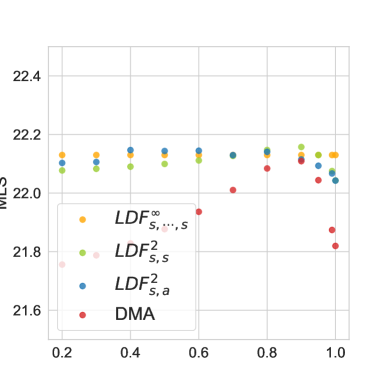
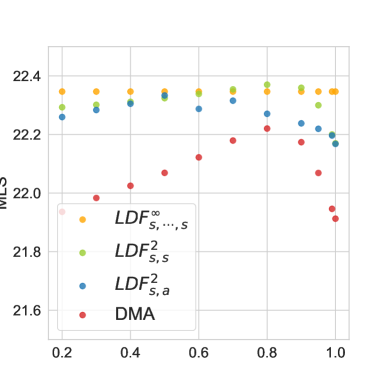
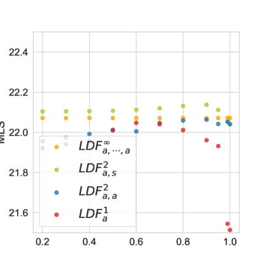
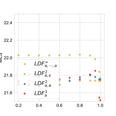
Figure 1: FX – MLS versus values of $\delta$ for LDF and $\alpha$ for DMA in the x-axis for the small and large model pool. The upper plots show the cases of model averaging whereas the lower plots show model selection.

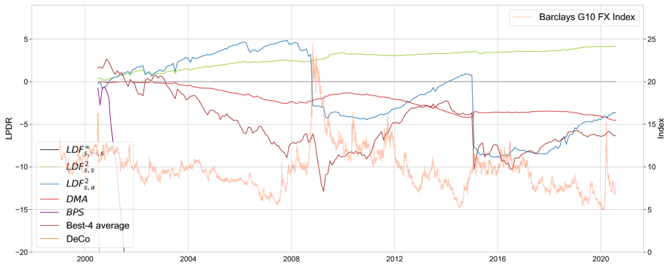
Figure 2: FX – LPDR for model averaging in the small model pool. $\mbox{LDF}_{\mbox{s},\mbox{s}}^{2}$ provides best performance robust to increases in the FX volatility.

In order to illustrate the time-dependent performance of the models we calibrated the models’ hyperparameters to the first 10 years of data. In Figure 2 we present the LPDR across time as compared to $\mbox{LDF}_{\mbox{s},\mbox{s}}^{2}$. We note that the competing models perform worse and the sudden drops in performance of $\mbox{LDF}_{\mbox{s},\mbox{a}}^{2}$ and Best-4 average models correspond to the period of big FX volatility increases as measured by Barclays G10 FX index.

2.2 Economic evaluation for model selection

Perform Markovitz portfolio selection where we want to maximise the expected returns given a constraint on the expected volatility. Here, we set this constraint to 10% annual vol.

In literature there are a few standard ways to evaluate portfolio performance.

• Money over time - this is usually a graph of how the money evolves over time after starting with 1 dollar on day 1. It’s quite effective but does not account for the fact that often the realised vol of strategies is not quite the same as the target vol and hence often the riskier strategies show up with larger fortune at the end.

• Sharpe ratio - which is the expectation of returns over time divide by vol of realised returns. This is a better evaluation metric and some authors even show the Sharpe ratio over time (question is whether one should use rolling or expanding window).

In this analysis we only consider LDF configurations that select a single model with single discounting, that is $\mbox{LDF}_{\mbox{a},\mbox{a}}^{2}$ and $\mbox{LDF}_{\mbox{a}}^{1}$. This is because the portfolio construction is targeted per model and any averaging effects would make the comparison invalid due to the correlation effects between the investment strategies.

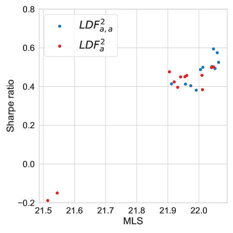
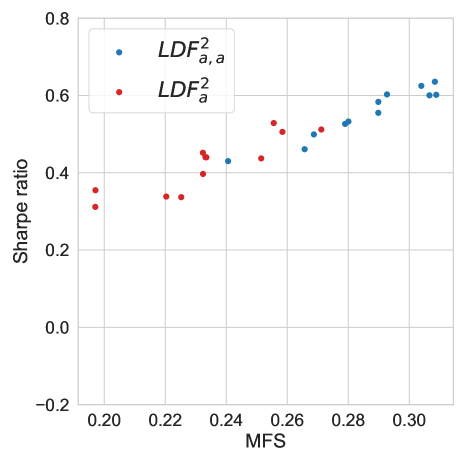
Figure 3: FX – mean score values versus achieves Sharpe ratios. In the left had side plot the log-scores were used, in the right hand side plot the focused scores were used.

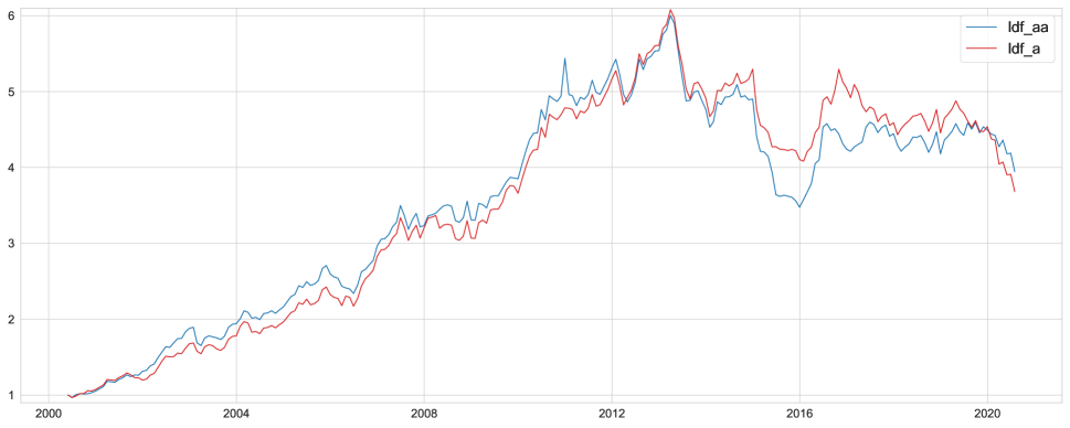
Figure 4: FX – Comparison for money over time for the two best performing models post factum in terms of log scores.

As shown in figure 1 the outperformance of $\mbox{LDF}_{\mbox{a},\mbox{a}}^{2}$ over $\mbox{LDF}_{\mbox{a}}^{1}$ is not large but it does translate to higher Sharpe ratio as shown in figure 3 and higher total wealth as show in figure 6.

For focused prediction, however, the differences in mean the mean scores are larger and translate directly to larger economic gains.

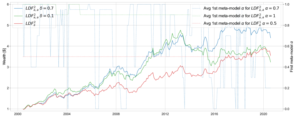
Figure 5: FX – Comparison for money over time for the two best performing models post factum in terms of focused scores.

Figure 6: FX – Portfolio composition for the best model as assessed by the focused prediction scores.