Improving Expert Predictions with Conformal Prediction
Abstract
Automated decision support systems promise to help human experts solve multiclass classification tasks more efficiently and accurately. However, existing systems typically require experts to understand when to cede agency to the system or when to exercise their own agency. Otherwise, the experts may be better off solving the classification tasks on their own. In this work, we develop an automated decision support system that, by design, does not require experts to understand when to trust the system to improve performance. Rather than providing (single) label predictions and letting experts decide when to trust these predictions, our system provides sets of label predictions constructed using conformal prediction—prediction sets—and forcefully asks experts to predict labels from these sets. By using conformal prediction, our system can precisely trade-off the probability that the true label is not in the prediction set, which determines how frequently our system will mislead the experts, and the size of the prediction set, which determines the difficulty of the classification task the experts need to solve using our system. In addition, we develop an efficient and near-optimal search method to find the conformal predictor under which the experts benefit the most from using our system. Simulation experiments using synthetic and real expert predictions demonstrate that our system may help experts make more accurate predictions and is robust to the accuracy of the classifier the conformal predictor relies on.
1 Introduction
In recent years, there has been an increasing interest in developing automated decision support systems to help human experts solve tasks in a wide range of critical domains, from medicine (Jiao et al.,, 2020) and drug discovery (Liu et al.,, 2021) to candidate screening (Wang et al.,, 2022) and criminal justice (Grgić-Hlača et al.,, 2019), to name a few. Among them, one of the main focuses has been multiclass classification tasks, where a decision support system uses a classifier to make label predictions and the experts decide when to follow the predictions made by the classifier (Bansal et al.,, 2019; Lubars and Tan,, 2019; Bordt and von Luxburg,, 2020).
However, these systems typically require human experts to understand when to trust a prediction made by the classifier. Otherwise, the experts may be better off solving the classification tasks on their own (Suresh et al.,, 2020). This follows from the fact that, in general, the accuracy of a classifier differs across data samples (Raghu et al.,, 2019). In this context, several recent studies have analyzed how factors such as model confidence, model explanations and overall model calibration modulate trust (Papenmeier et al.,, 2019; Wang and Yin,, 2021; Vodrahalli et al.,, 2022). Unfortunately, it is not yet clear how to make sure that the experts do not develop a misplaced trust that decreases their performance (Yin et al.,, 2019; Nourani et al.,, 2020; Zhang et al.,, 2020). In this work, we develop a decision support system for multiclass classification tasks that, by design, does not require experts to understand when to trust the system to improve their performance.
Our contributions. For each data sample, our decision support system provides a set of label predictions—a prediction set—and forcefully asks human experts to predict a label from this set111There are many systems used everyday by experts (e.g., pilots flying a plane) that, under normal operation, restrict their choices. This does not mean that, in extreme circumstances, the expert should not have the ability to essentially switch off the system.. We view this type of decision support system as more natural since, given a set of alternatives, experts tend to narrow down their options to a subset of them before making their final decision (Wright and Barbour,, 1977; Beach,, 1993; Ben-Akiva and Boccara,, 1995). In a way, our support system helps experts by automatically narrowing down their options for them, decreasing their cognitive load and allowing them to focus their attention where it is most needed. This could be particularly useful when the task is tedious or requires domain knowledge since it is difficult to outsource the task, and domain experts are often a scarce resource. In the context of clinical text annotation222Clinical text annotation is a task where medical experts aim to identify clinical concepts in medical notes and map them to labels in a large ontology., a recent empirical study has concluded that, in terms of the overall accuracy, it may be more beneficial to recommend a subset of options than a single option (Levy et al.,, 2021).
By using the theory of conformal prediction (Vovk et al.,, 2005; Angelopoulos and Bates,, 2021) to construct the above prediction set, our system can precisely control the trade-off between the probability that the true label is not in the prediction set, which determines how frequently our system will mislead an expert, and the size of the prediction set, which determines the difficulty of the classification task the expert needs to solve using our system. In this context, note that, if our system would not forcefully ask the expert to predict a label from the prediction set, it would not be able to have this level of control and good performance would depend on the expert developing a good sense on when to predict a label from the prediction set and when to predict a label from outside the set, as noted by Levy et al., (2021). In addition, given an estimator of the expert’s success probability for any of the possible prediction sets, we develop an efficient and near-optimal search method to find the conformal predictor under which the expert is guaranteed to achieve the greatest accuracy with high probability. In this context, we also propose a practical method to obtain such an estimator using the confusion matrix of the expert predictions in the original classification task and a given discrete choice model.
Finally, we perform simulation experiments using synthetic and real expert predictions on several multiclass classification tasks. The results demonstrate that our decision support system is robust to both the accuracy of the classifier and the estimator of the expert’s success probability it relies on—the competitive advantage it provides improves with their accuracy, and the human experts do not decrease their performance by using the system even if the classifier or the estimator are very inaccurate. Additionally, the results also show that, even if the classifiers that our system relies on have high accuracy, an expert using our system may achieve significantly higher accuracy than the classifiers on their own—in our experiments with real data, the relative reduction in misclassification probability is over %. Finally, by using our system, our results suggest that the expert would reduce their misclassification probability by %333 An open-source implementation of our system is available at https://github.com/Networks-Learning/improve-expert-predictions-conformal-prediction..
Further related work. Our work builds upon further related work on distribution-free uncertainty quantification, reliable classification and learning under algorithmic triage.
There exist three fundamental notions of distribution-free uncertainty quantification in the literature: calibration, confidence intervals, and prediction sets (Vovk et al.,, 2005; Balasubramanian et al.,, 2014; Gupta et al.,, 2020; Angelopoulos and Bates,, 2021). Our work is most closely related to the rapidly increasing literature on prediction sets (Romano et al.,, 2019, 2020; Angelopoulos et al.,, 2021; Podkopaev and Ramdas,, 2021), however, to the best of our knowledge, prediction sets have not been optimized to serve automated decision support systems such as ours. In this context, we acknowledge that Babbar et al., (2022) have also very recently proposed using prediction sets in decision support systems. However, in contrast to our work, for each data sample, they allow the expert to predict label values outside the recommended subset, i.e., to predict any alternative from the entire universe of alternatives, and do not optimize the probability that the true label belongs to the subset. As a result, their method is not directly comparable to ours444In our simulation experiments, we estimate the performance achieved by an expert using our system via a model-based estimator of the expert’s success probability. Therefore, to compare our system with the system by Babbar et al., (2022), we would need to model the expert’s success probability whenever the expert can predict any label given a prediction set, a problem for which discrete choice theory provides little guidance..
There is an extensive line of work on reliable or cautious classification (Del Coz et al.,, 2009; Liu et al.,, 2014; Yang et al.,, 2017; Mortier et al.,, 2021; Ma and Denoeux,, 2021; Nguyen and Hüllermeier,, 2021). Reliable classification aims to develop models that can provide set-valued predictions to account for the prediction uncertainty of a classifier. However, in this line of work, there are no human experts who make the final predictions given the set-valued predictions, in contrast with our work. Moreover, the set-valued predictions typically lack distribution-free guarantees.
Learning under algorithmic triage seeks the development of machine learning models that operate under different automation levels—models that make decisions for a given fraction of instances and leave the remaining ones to human experts (Raghu et al.,, 2019; Mozannar and Sontag,, 2020; De et al.,, 2020, 2021; Okati et al.,, 2021). This line of work has predominantly focused on supervised learning settings with a few very recent notable exceptions (Straitouri et al.,, 2021; Meresht et al.,, 2022). However, in this line of work, each sample is either predicted by the model or by the human expert. In contrast, in our work, the model helps the human predict each sample. That being said, it is worth noting that there may be classifiers, data distributions and conformal scores under which the optimal conformal predictor and the optimal triage policy coincide, i.e., the optimal conformal predictor does recommend a single label or the entire label set of labels.
2 Problem Formulation
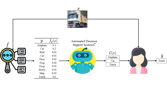
We consider a multiclass classification task where a human expert observes a feature vector555We denote random variables with capital letters and realizations of random variables with lower case letters. , with , and needs to predict a label , with . Then, our goal is to design an automated decision support system that, given a feature vector , helps the expert by automatically narrowing down the set of potential labels to a subset of them using a trained classifier that outputs scores for each class (e.g., softmax scores)666The assumption that is without loss of generality.. The higher the score , the more the classifier believes the true label . Here, we assume that, for each , the expert predicts a label among those in the subset according to an unknown policy . More formally, , where and denotes the probability simplex over the set of labels , and if . Refer to Figure 1 for an illustration of the automated decision support system we consider.
Ideally, we would like that, by design, the expert can only benefit from using the automated decision support system , i.e.,
| (1) |
where denotes the expert’s success probability if, for each , the human expert predicts a label among those in the subset . However, not all automated decision support systems fulfilling the above requirement will be equally useful—some will help experts increase their success probability more than others. For example, a system that always recommends for all satisfies Eq. 1. However, it is useless to the experts. Therefore, among those systems satisfying Eq. 1, we would like to find the system that helps the experts achieve the highest success probability777Note that maximizing the expert’s success probability is equivalent to minimizing the expected - loss . Considering other types of losses is left as an interesting avenue for future work., i.e.,
| (2) |
To address the design of such a system, we will look at the problem from the perspective of conformal prediction (Vovk et al.,, 2005; Angelopoulos and Bates,, 2021).
3 Subset Selection using Conformal Prediction
In general, if the trained classifier we use to build is not perfect, the true label may or may not be included in . In what follows, we will construct the subsets using the theory of conformal prediction. This will allow our system to be robust to the accuracy of the classifier it uses—the probability that the true label belongs to the subset will match almost exactly a given target probability with high probability, without making any distributional assumptions about the data distribution nor the classifier .
Let be a calibration set, where , be the conformal score888In general, the conformal score can be any function of and measuring the similarity between samples. (i.e., if the classifier is catastrophically wrong, the conformal score will be close to one), and be the empirical quantile of the conformal scores . Then, if we construct the subsets for new data samples as follows:
| (3) |
we have that the probability that the true label belongs to the subset conditionally on the calibration set is almost exactly with high probability as long as the size of the calibration set is sufficiently large. Specifically, we first note that the coverage probability is a random quantity999The randomness comes from the randomness of the calibration set sampling. whose distribution is given by the following proposition (refer to Appendix A.5 in Hulsman, (2022) for the proof):
Proposition 1
For a decision support system that constructs the subsets using Eq. 3, it holds that
| (4) |
as long as the conformal scores for all are almost surely distinct.
As an immediate consequence of Proposition 1, using the definition of the beta distribution, we have that
Moreover, given a target probability and tolerance values , we can compute the minimum size of the calibration set such that enjoys Probably Approximately Correct (PAC) coverage guarantees, i.e., with probability , it holds that Angelopoulos and Bates, (2021)
While the above coverage guarantee is valid for any choice of value, we would like to emphasize that there may be some values that will lead to larger gains in terms of success probability than others. Therefore, in what follows, our goal is to find the optimal that maximizes the expert’s success probability given a calibration set .
Remark. Most of the literature on conformal prediction focuses on the following conformal calibration guarantee (refer to Appendix D in Angelopoulos and Bates, (2021) for the proof):
Theorem 1
For an automated decision support system that constructs the subsets using Eq. 3, it holds that
where the probability is over the randomness in the sample it helps predicting and the calibration set used to compute the empirical quantile .
However, to afford the above marginal guarantee in our work, we would be unable to optimize the value to maximize the expert’ s success probability given a calibration set . This is because the guarantee requires that and are independent. That being said, in our experiments, we have empirically found that the optimal does not vary significantly across calibration sets, as shown in Appendix E.
4 Optimizing Across Conformal Predictors
We start by realizing that, given a calibration set , there only exist different conformal predictors. This is because the empirical quantile , which the subsets depend on, can only take different values. As a result, to find the optimal conformal predictor that maximizes the expert’s success probability, we need to solve the following maximization problem:
| (5) |
where , with , and the probability is only over the randomness in the samples the system helps predicting.
However, to find a near optimal solution to the above problem, we need to estimate the expert’s success probability . Assume for now that, for each , we have access to an estimator of the expert’s success probability such that, for any , with probability at least , it holds that . Then, we can use the following proposition to find a near-optimal solution to Eq. 5 with high probability:
Proposition 2
For any , consider an automated decision support system with
| (6) |
With probability at least , it holds that simultaneously.
More specifically, the above result directly implies that for any , with probability at least , it holds that:
| (7) |
Here, note that the above guarantees do not make use of the PAC coverage guarantees afforded by conformal prediction—they hold for any parameterized set-value predictor.
In what follows, we propose a practical method to estimate the expert’s success probability that builds upon the multinomial logit model (MNL), one of the most popular models in the vast literature on discrete choice models (Heiss,, 2016). More specifically, given a sample , we assume that the expert’s conditional success probability for the subset is given by
| (8) |
where denotes the expert’s preference for label value whenever the true label is . In the language of discrete choice models, one can view the true label as the context in which the expert chooses among alternatives (Tversky and Simonson,, 1993). In Appendix I, we consider and experiment with a more expressive context that, in addition to the true label, distinguishes between different levels of difficulty across data samples.
Further, to estimate the parameters , we assume we have access to (an estimation of) the confusion matrix for the expert predictions in the (original) multiclass classification task, similarly as in Kerrigan et al., (2021), i.e.,
and naturally set . Then, we can compute a Monte-Carlo estimator of the expert’s success probability using the above conditional success probability and an estimation set 101010The number of samples in and can differ. For simplicity, we assume both sets contain samples., i.e.,
| (9) |
Finally, for each , using Hoeffding’s inequality111111By using Hoeffding’s inequality, we derive a fairly conservative constant error bound for all values, however, we have experimentally found that, even with a relatively small amount of estimation and calibration data, our algorithm identifies near-optimal values, as shown in Figure 2. That being said, one could use tighter concentration inequalities such as Hoeffding–Bentkus and Waudby-Smith–Ramdas (Bates et al.,, 2021).,121212We are applying Hoeffding’s inequality only on the randomness of the samples , which are independent and identically distributed., we can conclude that, with probability at least , it holds that (refer to Appendix A.2):
| (10) |
As a consequence, as , converges to zero. This directly implies that the near-optimal converges to the true optimal and that, with probability at least , our system satisfies Eq. 1 asymptotically with respect to the number of samples in the estimation set.
Algorithm 1 summarizes the overall search method, where the function uses Eqs. 9 and 10. The algorithm first builds and then finds the near-optimal in . To build , it needs steps. To find the near-optimal , for each value and each sample , it needs to compute a subset . This is achieved by sorting the conformal scores and reusing computations across values, which takes steps. Therefore, the overall time complexity is .
Remarks. By using the MNL, we implicitly assume the independence of irrelevant alternatives (IIA) (Luce,, 1959), an axiom that states that the expert’s relative preference between two alternatives remains the same over all possible subsets containing these alternatives. While IIA is one of the most widely used axioms in the literature on discrete choice models, there is also a large body of experimental literature claiming to document real-world settings where IIA fails to hold (Tversky,, 1972; Huber et al.,, 1982; Simonson,, 1989). Fortunately, we have empirically found that experts may benefit from using our system even under strong violations of the IIA assumption in the estimator of the expert’s success probability (i.e., when the estimator of the expert’s success probability is not accurate), as shown in Figures 3 and 4.
Conformal prediction is one of many possible ways to construct set-valued predictors (Chzhen et al.,, 2021), i.e., predictors that, for each sample , output a set of label candidates . In our work, we favor conformal predictors over alternatives because they provably output trustworthy sets without making any assumption about the data distribution nor the classifier they rely upon. In fact, we can use conformal predictors with any off-the-shelf classifier. However, we would like to emphasize that our efficient search method (Algorithm 1) is rather generic and, together with an estimator of the expert’s success probability with provable guarantees, may be used to find a near-optimal set-valued predictor within a discrete set of set-valued predictors that maximizes the expert’s success probability. This is because our near-optimal guarantees in Proposition 2 do not make use of the PAC guarantees afforded by conformal prediction, as discussed previously. In Appendix D, we discuss an alternative set-valued predictor with PAC coverage guarantees, which may provide improved performance in scenarios where the classifier underpinning our system has not particularly high average accuracy. We hope our work will encourage others to develop set-valued predictors specifically designed to serve decision support systems.
| 0.3 | 0.5 | 0.7 | 0.9 | |
|---|---|---|---|---|
| 0.3 | 0.41 | 0.58 | 0.75 | 0.91 |
| 0.5 | 0.55 | 0.68 | 0.80 | 0.93 |
| 0.7 | 0.72 | 0.79 | 0.87 | 0.95 |
| 0.9 | 0.90 | 0.91 | 0.95 | 0.98 |
5 Experiments on Synthetic Data
In this section, we evaluate our system against the accuracy of the expert and the classifier, the size of the calibration and estimation sets, as well as the number of label values. Moreover, we analyze the robustness of our system to violations of the IIA assumption in the estimator of the expert’s success probability131313All algorithms ran on a Debian machine equipped with Intel Xeon E5-2667 v4 @ 3.2 GHz, 32GB memory and two M40 Nvidia Tesla GPU cards. See Appendix B for further details..
Experimental setup. We create a variety of synthetic prediction tasks, each with features per sample and a varying number of label values and difficulty. Refer to Appendix B for more details about the prediction tasks. For each prediction task, we generate samples, pick % of these samples at random as test set, which we use to estimate the performance of our system, and also randomly split the remaining % into three disjoint subsets for training, calibration, and estimation, whose sizes we vary across experiments. In each experiment, we specify the number of samples in the calibration and estimation sets—the remaining samples are used for training.
For each prediction task, we train a logistic regression model , which depending on the difficulty of the prediction task, achieves different success probability values . Moreover, we sample the expert’s predictions from the multinomial logit model defined by Eq. 8, with and , where is a parameter that controls the expert’s success probability , , for all , and is a normalization term. Finally, we repeat each experiment ten times and, each time, we sample different train, estimation, calibration, and test sets following the above procedure.
Experts always benefit from our system even if the classifier has low accuracy. We estimate the success probability achieved by four different experts, each with a different success probability , on four prediction tasks where the classifier achieves a different success probability . Table 1 summarizes the results, where each column corresponds to a different prediction task and each row corresponds to a different expert. We find that, using our system, the expert solves the prediction task significantly more accurately than the expert or the classifier on their own. Moreover, it is rather remarkable that, even if the classifier has low accuracy, the expert always benefits from using our system—in other words, our system is robust to the performance of the classifier it relies on. In Appendix C, we show qualitatively similar results for prediction tasks with other values of and .
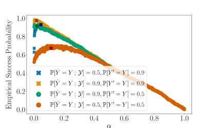
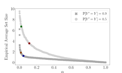
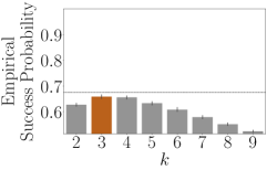
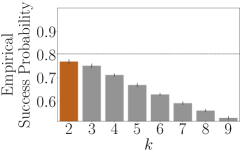
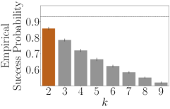
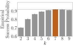
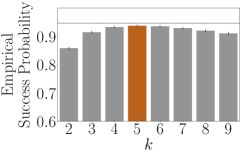
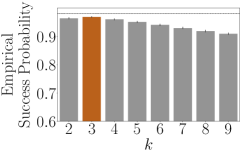
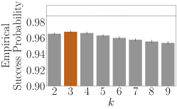
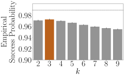
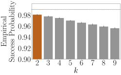
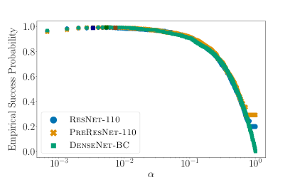
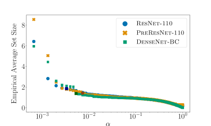
The performance of our system under found by Algorithm 1 and under is very similar. Given three prediction tasks where the expert and the classifier achieve different success probabilities and , we compare the performance of our system under the near-optimal found by Algorithm 1 and under all other possible values. Figure 2 summarizes the results, which suggest that: (i) the performance under is very close to that under , as suggested by Proposition 2; and, (ii) as long as , the performance of our system increases monotonically with respect to , however, once , the performance deteriorates as we increase . (iii) the higher the expert’s success probability , the smaller the near optimal and thus the greater the average size of the subsets . In Appendix G, we also show that, the smaller the near optimal , the greater the spread of the empirical distribution of the size of the subsets . We found qualitatively similar results using other expert-classifier pairs with different success probabilities.
Our system needs a relatively small amount of calibration and estimation data. We vary the amount of calibration and estimation data we feed into Algorithm 1 and, each time, estimate the expert’s success probability . Across prediction tasks, we consistently find that our system needs a relatively small amount of calibration and estimation data to perform well. For example, for all prediction tasks with label values and varying level of difficulty, the relative gain in empirical success probability achieved by an expert using our system with respect to an expert on their own, averaged across experts with , goes from for to for .
The greater the number of label values, the more an expert benefits from using our system. We consider prediction tasks with a varying number of label values, from to , and estimate the expert’s success probability for each task. Our results suggest that the relative gain in success probability, averaged across experts with , increases with the number of label values. For example, for , it goes from for to for . For other values, we found a similar trend.
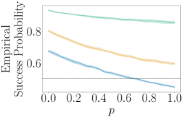


Our system is robust to strong violations of the IIA assumption in the estimator of the expert’s success probability. To study the robustness of our system to violations of the IIA assumption in the estimator of the expert’s success probability, we allow the expert’s preference for each label value in Eq. 8 to depend on the corresponding prediction set at test time. More specifically, we set
where is a parameter that controls the severity of the violation of the IIA assumption at test time. Here, note that if , the expert does not benefit from using our system as long as the prediction set , i.e., the expert’s conditional success probability is given by . Figure 3 summarizes the results, which show that our system is robust to (strong) violations of the IIA assumption in the estimator of the expert’s success probability.
| Classifier | |||
|---|---|---|---|
| ResNet-110 | 0.928 | 0.987 | 0.967 |
| PreResNet-110 | 0.944 | 0.989 | 0.972 |
| DenseNet | 0.964 | 0.990 | 0.980 |
6 Experiments on Real Data
In this section, we experiment with a dataset with real expert predictions on a multiclass classification task over natural images and several popular and highly accurate deep neural network classifiers. In doing so, we benchmark the performance of our system against a competitive top- set-valued predictor baseline, which always returns the label values with the highest scores, and analyze its robustness to violations of the IIA assumption in the estimator of the expert’s success probability. Here, we would like to explicitly note that we rely on the confusion matrix estimated using real expert predictions on the (original) multiclass classification task and the multinomial logit model defined by Eq. 8 to estimate the performance of our system and the competitive top- set-valued predictor baseline—no real experts actually used our decision support system.
Data description. We experiment with the dataset CIFAR-10H (Peterson et al.,, 2019), which contains natural images taken from the test set of the standard CIFAR-10 (Krizhevsky et al.,, 2009). Each of these images belongs to one of classes and contains approximately expert predictions 141414The dataset CIFAR-10H is among the only publicly available datasets (released under Creative Commons BY-NC-SA 4.0 license) that we found containing multiple expert predictions per sample, necessary to estimate , a relatively large number of samples, and more than two classes. However, since our methodology is rather general, our system may be useful in other applications.. Here, we randomly split the dataset into three disjoint subsets for calibration, estimation and test, whose sizes we vary across experiments. In each experiment, we use the test set to estimate the performance of our system and we specify the number of samples in the calibration and estimation sets—the remaining samples are used for testing.
Experimental setup. Rather than training a classifier, we use three popular and highly accurate deep neural network classifiers trained on CIFAR-10, namely ResNet-110 (He et al., 2016a, ), PreResNet-110 (He et al., 2016b, ) and DenseNet (Huang et al.,, 2017). Moreover, we use the human predictions to estimate the confusion matrix for the expert predictions in the (original) multiclass classification task (Kerrigan et al.,, 2021) and then sample the expert’s prediction from the multinomial logit model defined by Eq. 8 to both estimate the expert’s conditional success probabilities in Eq. 9 in Algorithm 1 and estimate the expert’s success probability during testing. In what follows, even though the expert’s performance during testing is estimated using the multinomial logit model, rather than using real predictions from experts using our system, we refer to (the performance of) such a simulated expert as an expert.
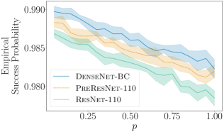
Performance evaluation. We start by estimating the success probability achieved by an expert using our system () and the best top- set-valued predictor (), which returns the label values with the highest scores151515 Appendix F shows the success probability achieved by an expert using the top- set-valued predictor for different values both for synthetic and real data.. Table 2 summarizes the results, where we also report the (empirical) success probability achieved by an expert solving the (original) multiclass task in their own. We find that, by allowing for recommended subsets of varying size, our system is consistently superior to the top- set-valued predictor. Moreover, we also find it very encouraging that, although the classifiers are highly accurate, our results suggest that an expert using our system can solve the prediction task significantly more accurately than the classifiers. More specifically, the relative reduction in misclassification probability goes from % (DenseNet) to % (ResNet-110). Finally, by using our system, our results suggest that the (average) expert would reduce their misclassification probability by %.
Robustness to violations of the IIA assumption in the estimator of the expert’s success probability. To study the robustness of our system to violations of the IIA assumption in the estimator of the expert’s success probability, we use the same experimental setting as in the synthetic experiments, where the parameter controls the severity of the violation of the IIA assumption at test time. Figure 4 summarizes the results for different values. It is remarkable that, even for highly accurate classifiers like the ones used for our experiments, the expert benefits from using our system even when . This is because, for accurate classifiers, many prediction sets are singletons containing the true label, as shown in Appendix H.
7 Conclusions
We have initiated the development of automated decision support systems that, by design, do not require human experts to understand when each of their recommendations is accurate to improve their performance with high probability. We have focused on multiclass classification and designed a system that, for each data sample, recommends a subset of labels to the experts using a classifier. Moreover, we have shown that our system can help experts make predictions more accurately and is robust to the accuracy of the classifier and the estimator of the expert’s success probability.
Our work opens up many interesting avenues for future work. For example, we have considered a simple, well-known conformal score function from the literature. However, it would be valuable to develop score functions especially designed for decision support systems. Moreover, it would be interesting to perform online estimation of the expert’s conditional success probability. Further, it would be important to investigate the ethical impact of our system, including human trust and bias, understand the robustness of our system to malicious attacks, and consider alternative performance metrics such as expert prediction time. Finally, it would be important to deploy and evaluate our system on a real-world application with human experts.
Acknowledgements
We would like to thank the anonymous reviewers for constructive feedback, which has helped improve our paper. Gomez-Rodriguez acknowledges support from the European Research Council (ERC) under the European Union’s Horizon 2020 research and innovation programme (grant agreement No. 945719). Wang acknowledges support from NSF Awards IIS-1901168 and IIS-2008139. All content represents the opinion of the authors, which is not necessarily shared or endorsed by their respective employers and/or sponsors.
References
- Angelopoulos et al., (2021) Angelopoulos, A., Bates, S., Malik, J., and Jordan, M. I. (2021). Uncertainty sets for image classifiers using conformal prediction. In International Conference on Learning Representations.
- Angelopoulos and Bates, (2021) Angelopoulos, A. N. and Bates, S. (2021). A gentle introduction to conformal prediction and distribution-free uncertainty quantification. arXiv preprint arXiv:2107.07511.
- Babbar et al., (2022) Babbar, V., Bhatt, U., and Weller, A. (2022). On the utility of prediction sets in human-ai teams. arXiv preprint arXiv:2205.01411.
- Balasubramanian et al., (2014) Balasubramanian, V., Ho, S.-S., and Vovk, V. (2014). Conformal prediction for reliable machine learning: theory, adaptations and applications. Newnes.
- Bansal et al., (2019) Bansal, G., Nushi, B., Kamar, E., Lasecki, W. S., Weld, D. S., and Horvitz, E. (2019). Beyond accuracy: The role of mental models in human-ai team performance. Proceedings of the AAAI Conference on Human Computation and Crowdsourcing, 7(1):2–11.
- Bates et al., (2021) Bates, S., Angelopoulos, A., Lei, L., Malik, J., and Jordan, M. (2021). Distribution-free, risk-controlling prediction sets. J. ACM, 68(6).
- Beach, (1993) Beach, L. R. (1993). Broadening the definition of decision making: The role of prechoice screening of options. Psychological Science, 4(4):215–220.
- Ben-Akiva and Boccara, (1995) Ben-Akiva, M. and Boccara, B. (1995). Discrete choice models with latent choice sets. International Journal of Research in Marketing, 12(1):9–24.
- Bordt and von Luxburg, (2020) Bordt, S. and von Luxburg, U. (2020). When humans and machines make joint decisions: A non-symmetric bandit model. arXiv preprint arXiv:2007.04800.
- Chzhen et al., (2021) Chzhen, E., Denis, C., Hebiri, M., and Lorieul, T. (2021). Set-valued classification–overview via a unified framework. arXiv preprint arXiv:2102.12318.
- De et al., (2020) De, A., Koley, P., Ganguly, N., and Gomez-Rodriguez, M. (2020). Regression under human assistance. In Proceedings of the AAAI Conference on Artificial Intelligence.
- De et al., (2021) De, A., Okati, N., Zarezade, A., and Gomez-Rodriguez, M. (2021). Classification under human assistance. In Proceedings of the AAAI Conference on Artificial Intelligence.
- Del Coz et al., (2009) Del Coz, J. J., Díez, J., and Bahamonde, A. (2009). Learning nondeterministic classifiers. Journal of Machine Learning Research, 10(10).
- Grgić-Hlača et al., (2019) Grgić-Hlača, N., Engel, C., and Gummadi, K. P. (2019). Human decision making with machine assistance: An experiment on bailing and jailing. Proceedings of the ACM on Human-Computer Interaction, 3(CSCW):1–25.
- Gupta et al., (2020) Gupta, C., Podkopaev, A., and Ramdas, A. (2020). Distribution-free binary classification: prediction sets, confidence intervals and calibration. In Advances in Neural Information Processing Systems.
- (16) He, K., Zhang, X., Ren, S., and Sun, J. (2016a). Deep residual learning for image recognition. In Proceedings of the IEEE conference on computer vision and pattern recognition, pages 770–778.
- (17) He, K., Zhang, X., Ren, S., and Sun, J. (2016b). Identity mappings in deep residual networks. In European conference on computer vision, pages 630–645. Springer.
- Heiss, (2016) Heiss, F. (2016). Discrete choice methods with simulation. Taylor & Francis.
- Huang et al., (2017) Huang, G., Liu, Z., Van Der Maaten, L., and Weinberger, K. Q. (2017). Densely connected convolutional networks. In 2017 IEEE Conference on Computer Vision and Pattern Recognition (CVPR), pages 2261–2269.
- Huber et al., (1982) Huber, J., Payne, J. W., and Puto, C. (1982). Adding asymmetrically dominated alternatives: Violations of regularity and the similarity hypothesis. Journal of consumer research, 9(1):90–98.
- Hulsman, (2022) Hulsman, R. (2022). Distribution-free finite-sample guarantees and split conformal prediction. arXiv preprint arXiv:2210.14735.
- Jiao et al., (2020) Jiao, W., Atwal, G., Polak, P., Karlic, R., Cuppen, E., Danyi, A., de Ridder, J., van Herpen, C., Lolkema, M. P., Steeghs, N., et al. (2020). A deep learning system accurately classifies primary and metastatic cancers using passenger mutation patterns. Nature communications, 11(1):1–12.
- Kerrigan et al., (2021) Kerrigan, G., Smyth, P., and Steyvers, M. (2021). Combining human predictions with model probabilities via confusion matrices and calibration. arXiv preprint arXiv:2109.14591.
- Krizhevsky et al., (2009) Krizhevsky, A., Hinton, G., et al. (2009). Learning multiple layers of features from tiny images. Citeseer.
- Levy et al., (2021) Levy, A., Agrawal, M., Satyanarayan, A., and Sontag, D. (2021). Assessing the impact of automated suggestions on decision making: Domain experts mediate model errors but take less initiative. In Proceedings of the 2021 CHI Conference on Human Factors in Computing Systems.
- Liu et al., (2021) Liu, R., Rizzo, S., Whipple, S., Pal, N., Pineda, A. L., Lu, M., Arnieri, B., Lu, Y., Capra, W., Copping, R., et al. (2021). Evaluating eligibility criteria of oncology trials using real-world data and ai. Nature, 592(7855):629–633.
- Liu et al., (2014) Liu, Z.-G., Pan, Q., Dezert, J., and Mercier, G. (2014). Credal classification rule for uncertain data based on belief functions. Pattern Recognition, 47(7):2532–2541.
- Lubars and Tan, (2019) Lubars, B. and Tan, C. (2019). Ask not what ai can do, but what ai should do: Towards a framework of task delegability. Advances in Neural Information Processing Systems, 32:57–67.
- Luce, (1959) Luce, R. D. (1959). On the possible psychophysical laws. Psychological review, 66(2):81.
- Ma and Denoeux, (2021) Ma, L. and Denoeux, T. (2021). Partial classification in the belief function framework. Knowledge-Based Systems, 214:106742.
- Meresht et al., (2022) Meresht, V. B., De, A., Singla, A., and Gomez-Rodriguez, M. (2022). Learning to switch among agents in a team. Transactions on Machine Learning Research.
- Mortier et al., (2021) Mortier, T., Wydmuch, M., Dembczyński, K., Hüllermeier, E., and Waegeman, W. (2021). Efficient set-valued prediction in multi-class classification. Data Mining and Knowledge Discovery, 35(4):1435–1469.
- Mozannar and Sontag, (2020) Mozannar, H. and Sontag, D. (2020). Consistent estimators for learning to defer to an expert. In International Conference on Machine Learning, pages 7076–7087.
- Nguyen and Hüllermeier, (2021) Nguyen, V.-L. and Hüllermeier, E. (2021). Multilabel classification with partial abstention: Bayes-optimal prediction under label independence. Journal of Artificial Intelligence Research, 72:613–665.
- Nourani et al., (2020) Nourani, M., King, J. T., and Ragan, E. D. (2020). The role of domain expertise in user trust and the impact of first impressions with intelligent systems. ArXiv, abs/2008.09100.
- Okati et al., (2021) Okati, N., De, A., and Gomez-Rodriguez, M. (2021). Differentiable learning under triage. In Advances in Neural Information Processing Systems.
- Papenmeier et al., (2019) Papenmeier, A., Englebienne, G., and Seifert, C. (2019). How model accuracy and explanation fidelity influence user trust. arXiv preprint arXiv:1907.12652.
- Peterson et al., (2019) Peterson, J. C., Battleday, R. M., Griffiths, T. L., and Russakovsky, O. (2019). Human uncertainty makes classification more robust. arXiv preprint arXiv:1908.07086.
- Podkopaev and Ramdas, (2021) Podkopaev, A. and Ramdas, A. (2021). Distribution-free uncertainty quantification for classification under label shift. In Proceedings of the 37th Conference on Uncertainty in Artificial Intelligence.
- Raghu et al., (2019) Raghu, M., Blumer, K., Corrado, G., Kleinberg, J., Obermeyer, Z., and Mullainathan, S. (2019). The algorithmic automation problem: Prediction, triage, and human effort. arXiv preprint arXiv:1903.12220.
- Romano et al., (2019) Romano, Y., Patterson, E., and Candes, E. (2019). Conformalized quantile regression. Advances in Neural Information Processing Systems, 32:3543–3553.
- Romano et al., (2020) Romano, Y., Sesia, M., and Candes, E. (2020). Classification with valid and adaptive coverage. Advances in Neural Information Processing Systems, 33:3581–3591.
- Simonson, (1989) Simonson, I. (1989). Choice based on reasons: The case of attraction and compromise effects. Journal of consumer research, 16(2):158–174.
- Straitouri et al., (2021) Straitouri, E., Singla, A., Meresht, V. B., and Gomez-Rodriguez, M. (2021). Reinforcement learning under algorithmic triage. arXiv preprint arXiv:2109.11328.
- Suresh et al., (2020) Suresh, H., Lao, N., and Liccardi, I. (2020). Misplaced trust: Measuring the interference of machine learning in human decision-making. In 12th ACM Conference on Web Science, pages 315–324.
- Tversky, (1972) Tversky, A. (1972). Elimination by aspects: A theory of choice. Psychological review, 79(4):281.
- Tversky and Simonson, (1993) Tversky, A. and Simonson, I. (1993). Context-dependent preferences. Management Science, 39(10):1179–1189.
- Vodrahalli et al., (2022) Vodrahalli, K., Gerstenberg, T., and Zou, J. (2022). Uncalibrated models can improve human-ai collaboration. In Advances in Neural Information Processing Systems.
- Vovk et al., (2005) Vovk, V., Gammerman, A., and Shafer, G. (2005). Algorithmic Learning in a Random World. Springer-Verlag, Berlin, Heidelberg.
- Wang et al., (2022) Wang, L., Joachims, T., and Gomez-Rodriguez, M. (2022). Improving screening processes via calibrated subset selection. In Proceedings of the 39th International Conference on Machine Learning.
- Wang and Yin, (2021) Wang, X. and Yin, M. (2021). Are explanations helpful? a comparative study of the effects of explanations in ai-assisted decision-making. In 26th International Conference on Intelligent User Interfaces, pages 318–328.
- Wright and Barbour, (1977) Wright, P. and Barbour, F. (1977). Phased decision strategies: Sequels to an initial screening. Graduate School of Business, Stanford University.
- Yang et al., (2017) Yang, G., Destercke, S., and Masson, M.-H. (2017). Cautious classification with nested dichotomies and imprecise probabilities. Soft Computing, 21(24):7447–7462.
- Yin et al., (2019) Yin, M., Wortman Vaughan, J., and Wallach, H. (2019). Understanding the effect of accuracy on trust in machine learning models. In Proceedings of the 2019 chi conference on human factors in computing systems, pages 1–12.
- Zhang et al., (2020) Zhang, Y., Liao, Q. V., and Bellamy, R. K. (2020). Effect of confidence and explanation on accuracy and trust calibration in ai-assisted decision making. In Proceedings of the 2020 Conference on Fairness, Accountability, and Transparency, pages 295–305.
Appendix A Proofs
A.1 Proof of Proposition 2
Given the estimators of , we have that, for each , it holds that
| (11) |
with probability at least . By applying the union bound, we know that the above events hold simultaneously for all with probability at least . Moreover, by rearranging, the above expression can be rewritten as
| (12) |
Let . For , with probability , it holds that for all ,
where the last inequality follows from Eq. 12.
A.2 Derivation of Error Expression for Hoeffding’s Inequality
From Hoeffding’s inequality we have that:
Theorem 2
Let be i.i.d., with and be the empirical estimate of . Then:
| (13) |
and
| (14) |
hold for all .
In our case we have and . Moreover, note that the expectation of is given by:
where the expectations are over the joint distribution of prediction sets and true labels .
Hence, for the empirical estimate of and its error :
| (15) |
and
| (16) |
hold. Further, if we set
| (17) |
then
| (18) |
and
| (19) |
hold for any . As follows, based on Eq. 17:
A.3 Proof of Proposition 3
We proceed similarly as in the Appendix A.5 in Hulsman, (2022). First, note that, by definition, we have that
where denotes the -th smallest conformal score in the calibration set . Then, as long as the conformal scores in the calibration set are almost surely distinct, it follows directly from Proposition 4 in Hulsman, (2022) that
| (20) |
where . Moreover, for any , we have that, by construction, if and only if . Then, Eq. 22 follows directly from Eq. 20.
Appendix B Implementation Details
To implement our algorithms and run all the experiments on synthetic and real data, we used PyTorch 1.12.1, NumPy 1.20.1 and Scikit-learn 1.0.2 on Python 3.9.2. For reproducibility, we use a fixed random seed in all random procedures. Moreover, we set everywhere.
Synthetic prediction tasks. We create different prediction tasks, where we vary the number of labels and the level of difficulty of the task. More specifically, for each value of , we create four different tasks of increasing difficulty where the success probability of the logistic regression classifier is , , and , respectively.
To create each task, we use the function make_classification of the Scikit-learn library. This function allows the creation of data for synthetic prediction tasks with very particular user-defined characteristics, through the generation of clusters of normally distributed points on the vertices of a multidimensional hypercube. The number of the dimensions of the hypercube indicates the number of informative features of each sample, which in our case we set at 15 for all prediction tasks. Linear combinations of points, i.e., the informative features, are used to create redundant features, the number of which we set at 5. The difficulty of the prediction task is controlled through the size of the hypercube, with a multiplicative factor, namely clas_sep, which we tuned accordingly for each value so that the success probability of the logistic regression classifier above spans a wide range of values across tasks. All the selected values of this parameter can be found in the configuration file config.py in the code. Finally, we set the proportion of the samples assigned to each label, i.e., the function parameter weights, using a Dirichlet distribution of order with parameters .
Appendix C Additional Synthetic Prediction Tasks, Number of Labels and Amount of Calibration and Estimation Data
To complement the results in Table 1 in the main paper, we experiment with additional prediction tasks with different number of labels and amount of calibration and estimation data . For each value of and , we estimate the success probability achieved by four different experts using our system, each with a different success probability , on four prediction tasks where the classifier achieves a different success probability . Figure 5 summarizes the results.
| 0.3 | 0.5 | 0.7 | 0.9 | |
|---|---|---|---|---|
| 0.3 | 0.56 | 0.72 | 0.84 | 0.94 |
| 0.5 | 0.68 | 0.80 | 0.89 | 0.95 |
| 0.7 | 0.79 | 0.87 | 0.93 | 0.97 |
| 0.9 | 0.92 | 0.95 | 0.97 | 0.99 |
| 0.3 | 0.5 | 0.7 | 0.9 | |
|---|---|---|---|---|
| 0.3 | 0.62 | 0.76 | 0.87 | 0.95 |
| 0.5 | 0.72 | 0.83 | 0.91 | 0.96 |
| 0.7 | 0.83 | 0.90 | 0.95 | 0.98 |
| 0.9 | 0.93 | 0.96 | 0.98 | 0.99 |
| 0.3 | 0.5 | 0.7 | 0.9 | |
|---|---|---|---|---|
| 0.3 | 0.42 | 0.58 | 0.75 | 0.91 |
| 0.5 | 0.55 | 0.66 | 0.80 | 0.93 |
| 0.7 | 0.72 | 0.79 | 0.87 | 0.96 |
| 0.9 | 0.90 | 0.92 | 0.94 | 0.98 |
| 0.3 | 0.5 | 0.7 | 0.9 | |
|---|---|---|---|---|
| 0.3 | 0.56 | 0.73 | 0.84 | 0.94 |
| 0.5 | 0.67 | 0.80 | 0.88 | 0.96 |
| 0.7 | 0.79 | 0.88 | 0.93 | 0.98 |
| 0.9 | 0.92 | 0.94 | 0.97 | 0.99 |
| 0.3 | 0.5 | 0.7 | 0.9 | |
|---|---|---|---|---|
| 0.3 | 0.62 | 0.77 | 0.87 | 0.95 |
| 0.5 | 0.73 | 0.83 | 0.91 | 0.97 |
| 0.7 | 0.83 | 0.89 | 0.95 | 0.98 |
| 0.9 | 0.93 | 0.96 | 0.98 | 0.99 |
Appendix D Beyond Standard Conformal Prediction
In Section 4, we have used standard conformal prediction (Angelopoulos and Bates,, 2021) to construct the recommended subsets —we have constructed by comparing the conformal scores to a single threshold , as shown in Eq. 3. Here, we introduce a set-valued predictor based on conformal prediction that constructs using two thresholds and . By doing so, the recommended subsets will include label values whose corresponding conformal scores are neither unreasonably large, as in standard conformal prediction, nor unreasonably low in comparison with the conformal scores of the samples in the calibration set . This may be useful in scenarios where the classifier underpinning our system has not particularly high average accuracy161616 In such scenarios, the conformal scores of the samples in the calibration set can occasionally have low values—otherwise, the classifier would be highly accurate—and thus it is beneficial to exclude label values with (very) low conformal scores from the recommended subsets—those label values the classifier is confidently wrong about..
More specifically, given a calibration set , let , with , and and be the and empirical quantiles of the conformal scores . If we construct the subsets for new data samples as follows:
| (21) |
we have that the probability that the true label belongs to the subset conditionally on the calibration set is almost exactly with high probability as long as the size of the calibration set is sufficiently large. More specifically, we first note that the coverage probability is a random quantity whose distribution is given by the following proposition, which is the counterpart of Proposition 1:
Proposition 3
For a decision support system that constructs using Eq. 21, as long as the conformal scores for all are almost surely distinct, it holds that:
| (22) |
where .
As an immediate consequence of Proposition 3, using the definition of the beta distribution, we have that
where . Moreover, given a target probability and tolerance values , we can compute the minimum size of the calibration set such that enjoys Probably Approximately Correct (PAC) coverage guarantees, i.e., with probability , it holds that
Finally, given an estimator of the expert’s success probability such that for each and , with probability at least , it holds that , we can proceed similarly as in standard conformal prediction to find the near optimal that maximizes the expert’s success probability with high probability, by using and . Here, it is worth pointing out that, in contrast with the case of standard conformal prediction, the time complexity of finding the near optimal and is . Moreover, we can still rely on the practical method to estimate the expert’s conditional success probability introduced in Section 4.
Appendix E Sensitivity to the Choice of Calibration Set
In this section, we repeat the experiments on synthetic and real data using independent realizations of the calibration, estimation and test sets. Then, for each data split, we compare the empirical coverage achieved by our system on the test set to the corresponding target coverage .
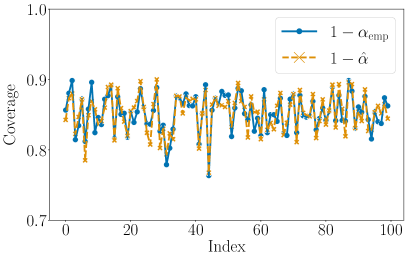
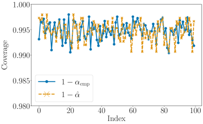
Figure 6 summarizes the results for (a) one synthetic prediction task and one synthetic expert and (b) one popular deep neural network classifier on the CIFAR-10H dataset. We find that the value of the near-optimal does not vary significantly across experiments (i.e., across calibration sets) and, for each experiment, the empirical coverage is very close to and typically higher than the target coverage . We found similar results for other expert-classifier pairs with different success probabilities.
Appendix F Success Probability Achieved by an Expert using Top- Set-Valued Predictors
In this section, we estimate the success probability achieved by an expert using the top- set-valued predictor for different values using both synthetic and real data. Figures 7 and 8 summarize the results, which show that, by allowing for recommended subsets of varying size, our system is consistently superior to the top- set-valued predictor across configurations. Moreover, the results on synthetic data also show that, the higher the expert’s success probability , the greater the optimal value (i.e., the greater the optimal size of the recommended subsets ). This latter observation is consistent with the behavior exhibited by our system, where the higher the expert’s success probability , the lower the value of the near-optimal and thus the greater the average size of the recommended subsets , as shown in Figure 9.
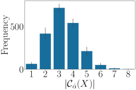
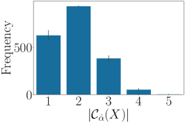
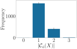
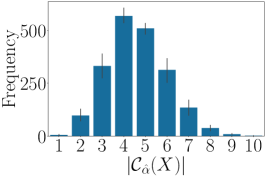
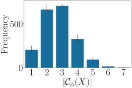
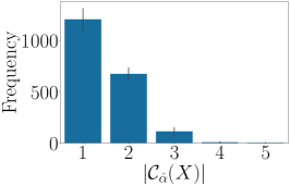
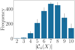
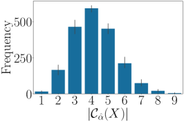
Appendix G Size Distribution of the Recommended Subsets
Figure 9 shows the empirical size distribution of the subsets recommended by our system during test for different experts and prediction tasks on synthetic data. The results show that, as the expert’s success probability increases and the near optimal decreases, the spread of the size distribution increases.
Appendix H Performance of Our System Under Different Values
In this section, we complement the results on CIFAR-10H dataset in the main paper by comparing, for each choice of classifier, the performance of our system under the near optimal found by Algorithm 1 and under all other possible values, including the optimal . Figure 10 summarizes the results, which suggest that, similarly as in the experiments on synthetic data, the performance of our system under and is very similar. However, since the classifiers are all highly accurate, the average size of the recommended subsets under and is quite close to one even though is much smaller than in the experiments in synthetic data.
Appendix I Additional Experiments using an Estimator of the Expert’s Success Probability with a More Expressive Context
In this section, we repeat the experiments on the CIFAR-10H dataset using an alternative discrete choice model with a more expressive context which, additionally to the true label, distinguishes between different levels of difficulty across data samples. The goal here is to show that our results are not an artifact of the choice of context used in the main paper.
We consider three increasing levels of difficulty, denoted as , , . The difficulty levels correspond to the 50% and 25% quantiles of the experts’ fractions of correct predictions per sample in the (original) multiclass classification task. Samples with a fraction of correct predictions larger than the 50% quantile belong to , those with a fraction of correct predictions smaller than the 25% quantile belong to , and the remaining ones belong to . Then, given a sample of difficulty , we assume that the expert’s conditional success probability for the subset is given by:
| (23) |
where denotes the expert preference for the label value whenever the true label is and the difficulty level of the sample is .
Further, to estimate the parameters , we resort to the conditional confusion matrix for the expert predictions on samples of difficulty , i.e., , and set . Finally, we compute a Monte-Carlo estimate of the expert’s success probability required by Algorithm 1 using the above conditional success probability and an estimation set , i.e.,
| (24) |
where denotes the difficulty level of .
Table 3 summarizes the results, which suggest that, in agreement with the main paper, an expert using our system may solve the prediction task significantly more accurately than the expert or the classifier on their own.
| Classifier | Expert using | |
|---|---|---|
| ResNet-110 | 0.928 | 0.981 |
| PreResNet-110 | 0.944 | 0.983 |
| DenseNet | 0.964 | 0.987 |
Finally, similarly as in the main paper, we also found that our system performs well with a small amount of calibration and estimation data—the relative gain in empirical success probability achieved by an expert using our system with respect to the same expert on their own raises from under to just under .