BCDAG: An R package for Bayesian structure and Causal learning of Gaussian DAGs

Abstract

Directed Acyclic Graphs (DAGs) provide a powerful framework to model causal relationships among variables in multivariate settings; in addition, through the do-calculus theory, they allow for the identification and estimation of causal effects between variables also from pure observational data. In this setting, the process of inferring the DAG structure from the data is referred to as causal structure learning or causal discovery. We introduce BCDAG, an R package for Bayesian causal discovery and causal effect estimation from Gaussian observational data, implementing the Markov chain Monte Carlo (MCMC) scheme proposed by Castelletti & Mascaro (2021). Our implementation scales efficiently with the number of observations and, whenever the DAGs are sufficiently sparse, with the number of variables in the dataset. The package also provides functions for convergence diagnostics and for visualizing and summarizing posterior inference. In this paper, we present the key features of the underlying methodology along with its implementation in BCDAG. We then illustrate the main functions and algorithms on both real and simulated datasets.

Keywords: Graphical model, Bayesian structure learning, Causal inference, Markov chain Monte Carlo, R

1 Introduction

In the last decades, probabilistic graphical models (Lauritzen, 1996) have emerged as a powerful tool for modelling and inferring dependence relations in complex multivariate settings. Specifically, Directed Acyclic Graphs (DAGs), also called Bayesian networks, adopt a graph-based representation to model a given set of conditional independence statements between variables which defines the DAG Markov property. In addition, if coupled with the do-calculus theory (Pearl, 2000), DAGs can be also adopted for causal inference and allow to identify and estimate causal relationships between variables. When DAGs are endowed with causal assumptions, the process of learning their graphical structure is usually referred to as causal structure learning or simply causal discovery (Peters et al., 2017) and often employed in a non-experimental setting, namely when only observational data are available; see Maathuis & Nandy (2016) for a review. In this setting, assuming faithfulness and causal sufficiency (Spirtes et al., 2000) it is possible to learn the DAG structure only up to its Markov equivalence class (Andersson et al., 1997), which collects all DAGs having the same Markov property. However, because equivalent DAGs still represent different Structural Causal Models (Pearl, 2000) (SCMs), a collection of potentially distinct causal effects can be recovered from the estimated Markov equivalence class (Maathuis et al., 2009).

The task of causal discovery has been tackled from different methodological perspectives, and in particular under both the frequentist and Bayesian frameworks. A primary distinction among frequentist methods is between constraint-based and score-based algorithms. The former include algorithms that recover the DAG-equivalence class through sequences of conditional independence tests. The most popular methods are the PC and Fast Causal Inference (FCI) algorithms (Spirtes et al., 2000), together with their extensions rankPC and rankFCI (Harris & Drton, 2013), based on more general (non-parametric) conditional independence tests. Differently, score-based methods implement a suitable score function which is maximized over the space of DAGs (or their equivalence classes) to provide a graph estimate; examples are the Greedy Equivalence Search (GES) algorithm of Chickering (2002) and the HC Bdeu method (Russell & Norvig, 2009). Going beyond this distinction, a variety of hybrid methods, i.e. combining features of both the two approaches, have been proposed; see for instance Tsamardinos et al. (2006), Solus et al. (2021) and Shimizu et al. (2006), the latter tailored to non-Gaussian linear structural equation models. For an extensive review of causal discovery methods the reader can refer to Heinze-Deml et al. (2018a).

R implementations of frequentist approaches for structure learning are available within a few packages, the most popular being bnlearn and pcalg. Specifically, bnlearn (Scutari, 2010) implements both structure learning and parameter estimation for discrete and Gaussian Bayesian networks. However, it is not specifically tailored to causal inference since it does not provide estimation of causal effects. On the other hand, pcalg (Kalisch et al., 2012) focuses on causal inference applications; it thus implements various algorithms for causal discovery from observational and experimental data (Heinze-Deml et al., 2018b; Hauser & Bühlmann, 2012) and causal effect estimation when the DAG is unknown (Maathuis et al., 2009; Nandy et al., 2017). Outside the R environment, Python implementations of causal discovery and causal inference methodologies are available within the Causal discovery toolbox of Kalainathan & Goudet (2019), causal-dag (Squires & Uhler, 2018) and causal-learn (Zhang et al., 2022), the last providing a Python extension of Tetrad (Glymour et al., 1988), the historical Java application for causal discovery.

On the Bayesian side, DAG structure learning has been traditionally tackled as a Bayesian model selection problem; in this framework the target is represented by the posterior distribution of graph structures which is typically approximated through Markov Chain Monte Carlo (MCMC) methods; see for instance Cooper & Herskovits (1992); Ni et al. (2017); Castelletti et al. (2018). Differently from frequentist methods, Bayesian techniques provide a coherent quantification of the uncertainty around DAG estimates. By converse however, they require the elicitation of a suitable parameter prior distribution for each candidate DAG-model. To this end, Heckerman et al. (1995) and Geiger & Heckerman (2002) proposed an effective procedure which assigns priors to DAG-model parameters via a small number of direct assessments and guarantees score equivalence for Markov equivalent DAGs. Most importantly the two methods, developed for categorical and Gaussian DAG-models respectively, lead to closed-form expressions for the DAG marginal likelihood, which serves as input to model selection algorithms based on MCMC schemes. More recently, Ben-David et al. (2015) and Cao et al. (2019) introduced multi-shape DAG-Wishart distributions as conjugate priors for Gaussian DAG-models. Accordingly, their framework also allows for posterior inference on model parameters, a feature which is also essential for causal effect estimation (Castelletti & Consonni, 2021b).

R implementations of Bayesian methods for DAG structure learning are provided by the packages mcmcabn and BiDAG (Suter et al., 2021) among a few others. The former develops structure MCMC algorithms to approximate a posterior distribution over DAGs, and is implemented for both discrete and continuous data. Differently, BiDAG implements order and partition MCMC algorithms in the hybrid approach of Kuipers et al. (2021) which has been shown to perform better in terms of convergence as the number of variables increases. Both packages are tailored to DAG-model selection only and do not provide any implementation of methods for parameter estimation and causal inference. To our knowledge, no implementation of Bayesian methods for causal inference based on DAGs is available.

In this context we introduce BCDAG, an R package (R Core Team, 2021) for Bayesian structure learning and causal effect estimation from observational Gaussian data. BCDAG implements an efficient Partial Analytic Structure algorithm (Godsill, 2012) to sample from the joint posterior distribution of DAGs and DAG parameters and applies the Bayesian approach of Castelletti & Mascaro (2021) for causal effect estimation. Accordingly, our package combines i) structure learning of Gaussian DAGs, ii) posterior inference of DAG-model parameters and iii) estimation of causal effects between variables in the dataset.

The rest of the paper is organized as follows. In Section 2 we introduce Gaussian DAG-models from a Bayesian perspective. Specifically, we write the likelihood and define suitable prior distributions for both DAG structures and DAG-model parameters. In the same section we also summarize a few useful results regarding parameter posterior distributions and DAG marginal likelihoods. We then provide in Section 3 the definition of causal effect in a Gaussian-DAG setting. Section 4 presents the main MCMC scheme that we adopt for posterior inference of DAGs and parameters and in turn for causal effect estimation. Illustrations of the main functions and algorithms are provided throughout the paper and described more extensively in Section 5 on both simulated and real data. Finally, Section 6 presents a brief discussion.

2 Gaussian DAG-models

Let $\mathcal{D}=(V,E)$ be a Directed Acyclic Graph (DAG), where $V=\{1,\dots,q\}$ is a set of vertices (or nodes) and $E\subseteq V\times V$ a set of edges. If $(u,v)\in E$ then $\mathcal{D}$ contains the directed edge $u\rightarrow v$. In addition, $\mathcal{D}$ cannot contain cycles, that is paths of the form $u_{0}\rightarrow u_{1}\rightarrow\dots\rightarrow u_{k}$ where $u_{0}\equiv u_{k}$. For a given node $v$, if $u\rightarrow v\in E$ we say that $u$ is a parent of $v$; conversely $v$ is a child of $u$. The set of all parents of $v$ in $\mathcal{D}$ is denoted by $\mathrm{pa}_{\mathcal{D}}(v)$, while the set $\mathrm{fa}_{\mathcal{D}}(v)=v\cup\mathrm{pa}_{\mathcal{D}}(v)$ is called the family of $v$ in $\mathcal{D}$. Furthermore, a DAG is complete if all its nodes are joined by edges. Finally, a DAG $\mathcal{D}$ can be uniquely represented through its $(q,q)$ adjacency matrix $\bm{A}^{\mathcal{D}}$ such that $\bm{A}^{\mathcal{D}}_{u,v}=1$ if and only $\mathcal{D}$ contains $u\rightarrow v$ and $0$ otherwise.

A DAG $\mathcal{D}$ encodes a set of conditional independencies between nodes (variables) that can be read-off from the DAG using graphical criteria, such as d-separation (Pearl, 2000). The resulting set of conditional independencies embedded in $\mathcal{D}$ defines the DAG Markov property.

In the next sections we define a Gaussian DAG-model in terms of likelihood and prior distributions for model parameters. Preliminary results and functions needed for the MCMC algorithm presented in Section 4 are also introduced.

2.1 Likelihood

Let $\mathcal{D}=(V,E)$ be a DAG, $(X_{1},\dots,X_{q})$ a collection of real-valued random variables each associated to a node in $V$. We assume that the joint density of $(X_{1},\dots,X_{q})$ belongs to a zero-mean Gaussian DAG-model, namely

$$X_{1},\dots,X_{q}\,|\,\bm{\Omega}_{\mathcal{D}}\sim\mathcal{N}_{q}(\bm{0},\bm{\Omega}_{\mathcal{D}}^{-1}),\quad\bm{\Omega}_{\mathcal{D}}\in\mathcal{P}_{\mathcal{D}},$$ (1)

where $\bm{\Omega}_{\mathcal{D}}=\bm{\Sigma}_{\mathcal{D}}^{-1}$ is the precision (inverse-covariance) matrix, and $\mathcal{P}_{\mathcal{D}}$ is the space of symmetric positive definite (s.p.d.) precision matrices Markov w.r.t. $\mathcal{D}$. Accordingly, $\bm{\Omega}_{\mathcal{D}}$ satisfies the conditional independencies (Markov property) encoded by $\mathcal{D}$. For the remainder of this section we will assume the DAG fixed and therefore omit the dependence on $\mathcal{D}$ from the DAG-parameter $\bm{\Omega}_{\mathcal{D}}$.

An alternative representation of model (1) is given by the allied Structural Equation Model (SEM). Specifically, let $\bm{L}$ be a $(q,q)$ matrix of coefficients such that for each $(u,v)$-element $\bm{L}_{uv}$ with $u\neq v$, $\bm{L}_{uv}\neq 0$ if and only if $(u,v)\in E$, while $\bm{L}_{uu}=1$ for each $u=1,\dots,q$. Let also $\bm{D}$ be a $(q,q)$ diagonal matrix with $(u,u)$-element $\bm{D}_{uu}$. The SEM representation of (1) is then

$$\bm{L}^{\top}(X_{1},\dots,X_{q})^{\top}=\boldsymbol{\varepsilon},\quad\boldsymbol{\varepsilon}\sim\mathcal{N}_{q}(\bm{0},\bm{D}),$$ (2)

which implies the re-parameterization $\bm{\Omega}=\bm{L}\bm{D}^{-1}\bm{L}^{\top}$. The latter equality is sometimes referred to as the modified Cholesky decomposition of $\bm{\Omega}$ (Cao et al., 2019) and induces a re-parametrization of $\bm{\Omega}=\bm{\Sigma}^{-1}$ in terms of node-parameters $\big{\{}(\bm{D}_{jj},\bm{L}_{\prec j\,]}),\,j=1,\dots,q\big{\}}$, such that

$$\bm{L}_{\prec j\,]}=-\bm{\Sigma}_{\prec j\,\succ}^{-1}\bm{\Sigma}_{\prec j\,]},\quad\bm{D}_{jj}=\bm{\Sigma}_{jj|\mathrm{pa}_{\mathcal{D}}(j)},$$

where $\bm{\Sigma}_{jj|\mathrm{pa}_{\mathcal{D}}(j)}=\bm{\Sigma}_{jj}-\bm{\Sigma}_{[\,j\succ}\bm{\Sigma}^{-1}_{\prec j\succ}\bm{\Sigma}_{\prec j\,]}$, $\prec j\,]=\mathrm{pa}_{\mathcal{D}}(j)\times j$, $[\,j\succ\,=j\times\mathrm{pa}_{\mathcal{D}}(j)$, $\prec j\succ\,=\mathrm{pa}_{\mathcal{D}}(j)\times\mathrm{pa}_{\mathcal{D}}(j)$. In particular, parameter $\bm{D}_{jj}$ corresponds to the conditional variance of $X_{j}$, $\mathbb{V}\!\mathrm{ar}(X_{j}\,|\,\bm{x}_{\mathrm{pa}_{\mathcal{D}}(j)})$. Base on (2), model (1) can be equivalently re-written as

$$f(x_{1},\dots,x_{q}\,|\,\bm{D},\bm{L})=\prod_{j=1}^{q}d\,\mathcal{N}(x_{j}\,|\,-\bm{L}_{\prec j\,]}^{\top}\bm{x}_{\mathrm{pa}_{\mathcal{D}}(j)},\bm{D}_{jj}).$$ (3)

Consider now $n$ independent samples $\bm{x}_{i}=(x_{i,1},\dots,x_{i,q})^{\top}$, $i=1,\dots,n$, from (3), and let $\bm{X}$ be the $(n,q)$ data matrix, row-binding of $\bm{x}_{i},\dots,\bm{x}_{n}$. The likelihood function is then

$$\begin{aligned} f(\bm{X}\,|\,\bm{D},\bm{L})&=\prod_{i=1}^{n}f(x_{i,1},\dots,x_{i,q}\,|\,\bm{D},\bm{L})\\ &=\prod_{j=1}^{q}d\,\mathcal{N}_{n}(\bm{X}_{j}\,|\,-\bm{X}_{\mathrm{pa}_{\mathcal{D}}(j)}\bm{L}_{\prec j\,]},\bm{D}_{jj}\bm{I}_{n}),\end{aligned}$$ (4)

where $\bm{X}_{A}$ is the $(n,|A|)$ sub-matrix of $\bm{X}$ corresponding to the set $A$ of columns of $\bm{X}$ and $\bm{I}_{n}$ denotes the $(n,n)$ identity matrix. We now proceed by assigning a suitable prior distribution to the DAG-dependent parameters $(\bm{D},\bm{L})$.

2.2 DAG-Wishart prior

Let $\bm{\Omega}$ be the precision matrix Markov w.r.t. to DAG $\mathcal{D}$. Conditionally on $\mathcal{D}$, we assign a prior to $\bm{\Omega}$ through a DAG-Wishart prior on $(\bm{D},\bm{L})$ with rate hyperparameter $\bm{U}$ (a $q\times q$ s.p.d. matrix) and shape hyperparameter $\boldsymbol{a}^{\mathcal{D}}=(a_{1}^{\mathcal{D}},\dots,a_{q}^{\mathcal{D}})^{\top}$ (Ben-David et al., 2015). An important feature of the DAG-Wishart distribution is that node-parameters $\big{\{}(\bm{D}_{jj},\bm{L}_{\prec j\,]}),\,j=1,\dots,q\big{\}}$ are a priori independent with distribution

$$\begin{aligned} \bm{D}_{jj}\,|\,\mathcal{D}\sim&\,\,\,\textnormal{I-Ga}\left(\frac{1}{2}a_{j}^{\mathcal{D}},\frac{1}{2}\bm{U}_{jj|\mathrm{pa}_{\mathcal{D}}(j)}\right),\\ \bm{L}_{\prec j\,]}\,|\,\bm{D}_{jj},\mathcal{D}\sim&\,\,\,\mathcal{N}_{|\mathrm{pa}_{\mathcal{D}}(j)|}\left(-\bm{U}_{\prec j\succ}^{-1}\bm{U}_{\prec j\,]},\bm{D}_{jj}\bm{U}_{\prec j\succ}^{-1}\right),\end{aligned}$$ (5)

where $\textnormal{I-Ga}(\alpha,\beta)$ stands for an Inverse-Gamma distribution with shape $\alpha>0$ and rate $\beta>0$ having expectation $\beta/(\alpha-1)$ ($\alpha>1$). Parameters $a_{1}^{\mathcal{D}},\dots,a_{q}^{\mathcal{D}}$ are specific to the DAG-model under consideration. The default choice, hereinafter considered, $a_{j}^{\mathcal{D}}=a+|\mathrm{pa}_{\mathcal{D}}(j)|-q+1$ $(a>q-1)$ guarantees compatibility among prior distributions for Markov equivalent DAGs. In particular, it can be shown that under this choice any two Markov equivalent DAGs are assigned the same marginal likelihood; see also Section 2.5. A prior on parameters $(\bm{D},\bm{L})$ is then given by

$$p(\bm{D},\bm{L}\,|\,\mathcal{D})=\prod_{j=1}^{q}p(\bm{L}_{\prec j\,]}\,|\,\bm{D}_{jj})\,p(\bm{D}_{jj}).$$ (6)

We refer to the resulting prior as the compatible DAG-Wishart distribution; see in particular Peluso & Consonni (2020) for full details.

2.3 Sampling from DAG-Wishart distributions

Given the results summarized in the previous section, Algorithm 1 implements a direct sampling from a compatible DAG-Wishart distribution.

Input: $n$, $\mathcal{D}$, $a$, $\bm{U}$

Output: $n$ draws from a compatible DAG-Wishart distribution with parameters $a,\bm{U}$

1

2 Set $a_{j}^{\mathcal{D}}=a+|\mathrm{pa}_{\mathcal{D}}(j)|-q+1$ for $j=1,\dots,q$

3 for $i=1,\dots,n$ do

4       Set $\bm{D}^{(i)}=\boldsymbol{0}_{q}$ a $(q,q)$ null matrix, $\bm{L}^{(i)}=\boldsymbol{I}_{q}$ a $(q,q)$ identity matrix

5       for $j=1,\dots,q$ do

6             Randomly draw elements $\big{(}\bm{D}_{jj}^{(i)},\bm{L}^{(i)}_{\prec j\,]}\big{)}$ from distributions in (5)

7       end for

8      

9 end for

10

return $\big{\{}\bm{D}^{(i)},\bm{L}^{(i)}\big{\}},\dots,\big{\{}\bm{D}^{(n)},\bm{L}^{(n)}\big{\}}$

Algorithm 1 Sampling from a DAG-Wishart distribution

Algorithm 1 is implemented within our package in the function rDAGWishart(n, DAG, a, U). Arguments of the function are:

• n: the number of draws;

• DAG: the $(q,q)$ adjacency matrix of DAG $\mathcal{D}$;

• a: the common shape hyperparameter of the DAG-Wishart distribution, $a>q-1$;

• U: the rate hyperparameter of the DAG-Wishart distribution, a $(q,q)$ s.p.d. matrix.

Consider the following example with $q=4$ variables and a DAG structure corresponding to DAG $\mathcal{D}$ in Figure 1.

Ψq <- 4
ΨDAG <- matrix(c(0,1,1,0,0,0,0,1,0,0,0,1,0,0,0,0), nrow = q)
ΨDAG
Ψ     [,1] [,2] [,3] [,4]
Ψ[1,]    0    0    0    0
Ψ[2,]    1    0    0    0
Ψ[3,]    1    0    0    0
Ψ[4,]    0    1    1    0
Ψ
ΨoutDL <- rDAGWishart(n = 1, DAG = DAG, a = q, U = diag(1, q))
Ψ
ΨoutDL$D
Ψ          [,1]      [,2]     [,3]     [,4]
Ψ[1,] 0.9651437 0.0000000 0.000000 0.000000
Ψ[2,] 0.0000000 0.2840032 0.000000 0.000000
Ψ[3,] 0.0000000 0.0000000 1.188965 0.000000
Ψ[4,] 0.0000000 0.0000000 0.000000 5.890211
Ψ
ΨoutDL$L
Ψ          [,1]        [,2]      [,3] [,4]
Ψ[1,]  1.000000  0.00000000  0.000000    0
Ψ[2,]  1.169280  1.00000000  0.000000    0
Ψ[3,] -1.659849  0.00000000  1.000000    0
Ψ[4,]  0.000000 -0.05807009 -1.379419    1

Matrices D and L represent one draw from a compatible DAG-Wishart distribution with parameters $a=q$, $U=\bm{I}_{q}$ and DAG structure represented by object DAG.

2.4 DAG-Wishart posterior

Because of conjugacy of (5) with the likelihood (4), the posterior distribution of $(\bm{D},\bm{L})$ given the data $\bm{X}$, $p(\bm{D},\bm{L}\,|\,\mathcal{D},\bm{X})$, is such that for $j=1,\dots,q$

$$\begin{aligned} \bm{D}_{jj}\,|\,\mathcal{D},\bm{X}\sim&\,\,\,\textnormal{I-Ga}\left(\frac{1}{2}\widetilde{a}_{j}^{\mathcal{D}},\frac{1}{2}\widetilde{\bm{U}}_{jj|\mathrm{pa}_{\mathcal{D}}(j)}\right),\\ \bm{L}_{\prec j\,]}\,|\,\bm{D}_{jj},\mathcal{D},\bm{X}\sim&\,\,\,\mathcal{N}_{|\mathrm{pa}_{\mathcal{D}}(j)|}\left(-\widetilde{\bm{U}}_{\prec j\succ}^{-1}\widetilde{\bm{U}}_{\prec j\,]},\bm{D}_{jj}\widetilde{\bm{U}}_{\prec j\succ}^{-1}\right),\end{aligned}$$ (7)

where $\widetilde{a}_{j}^{\mathcal{D}}=\widetilde{a}+|\mathrm{pa}_{\mathcal{D}}(j)|-q+1$, $\widetilde{a}=a+n$ and $\widetilde{\bm{U}}=\,\bm{U}+\bm{X}^{\top}\bm{X}.$ As a consequence, direct sampling from a DAG-Wishart posterior can be done using the rDAGWishart function simply by setting the input shape and rate parameters a,U as $\widetilde{a}$ and $\widetilde{\bm{U}}$ respectively.

2.5 DAG marginal likelihood

Finally, because of parameter prior independence in (6), the marginal likelihood of DAG $\mathcal{D}$ admits the same node-by-node factorization of (4), namely

$$\begin{aligned} m(\bm{X}\,|\,\mathcal{D})&=\int f(\bm{X}\,|\,\bm{D},\bm{L},\mathcal{D})\,p(\bm{D},\bm{L}\,|\,\mathcal{D})\,d(\bm{D},\bm{L})\\ &=\prod_{j=1}^{q}m(\bm{X}_{j}\,|\,\bm{X}_{\mathrm{pa}_{\mathcal{D}}(j)},\mathcal{D}).\end{aligned}$$ (8)

In addition, because of conjugacy of the priors $p(\bm{D}_{jj},\bm{L}_{\prec j\,]})$ with the Normal densities $d\,\mathcal{N}_{n}(\bm{X}_{j}\,|\,\cdot)$ in (4), each term $m(\bm{X}_{j}\,|\,\bm{X}_{\mathrm{pa}_{\mathcal{D}}(j)},\mathcal{D})$ can be obtained in closed-form expression from the ratio of prior and posterior normalizing constants as

$$m(\bm{X}_{j}\,|\,\bm{X}_{\mathrm{pa}_{\mathcal{D}}(j)},\mathcal{D})=(2\pi)^{-\frac{n}{2}}\cdot\frac{\big{|}\bm{U}_{\prec j\succ}\big{|}^{\frac{1}{2}}}{\big{|}\widetilde{\bm{U}}_{\prec j\succ}\big{|}^{\frac{1}{2}}}\cdot\frac{\Gamma\left(\frac{1}{2}\widetilde{a}_{j}^{\mathcal{D}}\right)}{\Gamma\left(\frac{1}{2}a_{j}^{\mathcal{D}}\right)}\cdot\frac{\Big{(}\frac{1}{2}\bm{U}_{jj\,|\,\mathrm{pa}_{\mathcal{D}}(j)}\Big{)}^{\frac{1}{2}a_{j}^{\mathcal{D}}}}{\left(\frac{1}{2}\widetilde{\bm{U}}_{jj\,|\,\mathrm{pa}_{\mathcal{D}}(j)}\right)^{\frac{1}{2}\widetilde{a}_{j}^{\mathcal{D}}}};$$ (9)

Equation (9) is implemented in the internal function DW_nodelml(node, DAG, tXX, n, a, U) which returns the logarithm of the node-marginal likelihood $m(\bm{X}_{j}\,|\,\bm{X}_{\mathrm{pa}_{\mathcal{D}}(j)},\mathcal{D})$. Arguments of the function are:

• node: the node $j$;

• DAG: the adjacency matrix of the underlying DAG $\mathcal{D}$;

• tXX: the $(q,q)$ matrix $\bm{X}^{\top}\bm{X}$;

• n: the sample size $n$;

• a,U: the shape and rate hyperparameters of the compatible DAG-Wishart prior.

2.6 Prior on DAGs

To complete our Bayesian model specification, we finally assign a prior to each DAG $\mathcal{D}\in\mathcal{S}_{q}$, the set of all DAGs on $q$ nodes. Specifically, we define a prior on $\mathcal{D}$ through independent Bernoulli distributions on the elements of the skeleton (underlying undirected graph) of $\mathcal{D}$. To this end, let $\bm{S}^{\mathcal{D}}$ be the (symmetric) $0-1$ adjacency matrix of the skeleton of $\mathcal{D}$ whose $(u,v)$-element is denoted by $\bm{S}^{\mathcal{D}}_{u,v}$. For a given prior probability of edge inclusion $\pi\in[0,1]$, we first assign a Bernoulli prior independently to each element $\bm{S}^{\mathcal{D}}_{u,v}$ belonging to the lower-triangular part of $\bm{S}^{\mathcal{D}}$, that is $\bm{S}^{\mathcal{D}}_{u,v}\,\stackrel{{\scriptstyle iid}}{{\sim}}\,\textnormal{Ber}(\pi),u>v$. As a consequence we obtain

$$p(\bm{S}^{\mathcal{D}})=\pi^{|\bm{S}^{\mathcal{D}}|}(1-\pi)^{\frac{q(q-1)}{2}-|\bm{S}^{\mathcal{D}}|},$$ (10)

where $|\bm{S}^{\mathcal{D}}|$ denotes the number of edges in the skeleton, or equivalently the number of entries equal to one in the lower-triangular part of $\bm{S}^{\mathcal{D}}$. Finally, we set $p(\mathcal{D})\propto p(\bm{S}^{\mathcal{D}})$ for $\mathcal{D}\in\mathcal{S}_{q}$.

3 Causal effects

In this section we summarize the definition of causal effect based on the do-calculus theory (Pearl, 2000). Let $I\subseteq V$ be an intervention target. A hard intervention on the set of variables $\{X_{j},\,j\in I\}$ is denoted by $\textnormal{do}\{X_{j}=\tilde{x}_{j}\}_{j\in I}$ and consists in the action of fixing each $X_{j}$, $j\in I$, to some chosen value $\tilde{x}_{j}$. Graphically, the effect of an intervention on variables in $I$ is represented through the so-called intervention DAG of $\mathcal{D}$, $\mathcal{D}^{I}$, which is obtained by removing all edges $(u,j)$ in $\mathcal{D}$ such that $j\in I$. Under the Gaussian assumption (3), the consequent post-intervention distribution can be written using the following truncated factorization

$$f(\bm{x}\,|\,\textnormal{do}\{X_{j}=\tilde{x}_{j}\}_{j\in I},\bm{D},\bm{L})=\begin{cases}\prod\limits_{i\notin I}d\,\mathcal{N}\big{(}x_{i}\,|\,-\bm{L}_{\prec i\,]}^{\top}\bm{x}_{\mathrm{pa}_{\mathcal{D}}(i)},\bm{D}_{jj}\big{)}\big{|}_{\{x_{j}=\tilde{x}_{j}\}_{j\in I}}&\text{if }x_{j}=\tilde{x}_{j}\,\,\forall j\in I,\\ \,\,0&\text{otherwise};\end{cases}$$ (11)

see also Pearl (2000) and Maathuis et al. (2009) for details. For a given “response” variable $Y\in\{X_{1},\dots,X_{q}\}$, Nandy et al. (2017) define the total joint effect of an intervention $\text{do}\{X_{j}=\tilde{x}_{j}\}_{j\in I}$ on $Y$ as

$$\bm{\theta}_{Y}^{I}:=\big{(}\theta_{h,Y}^{I}\big{)}_{h\in I},$$ (12)

where, for each $h\in I$,

$$\theta_{h,Y}^{I}:=\frac{\partial}{\partial{x_{h}}}\mathbb{E}\big{(}Y\,|\,\text{do}\{X_{j}=\tilde{x}_{j}\}_{j\in I}\big{)}$$ (13)

is the causal effect on $Y$ associated to variable $X_{h}$ in the joint intervention. In the Gaussian setting of Equation (11) we obtain

$$X_{1},\dots,X_{q}\,|\,\textnormal{do}\{X_{j}=\tilde{x}_{j}\}_{j\in I},\bm{\Omega}\,\sim\,\mathcal{N}_{q}\big{(}\bm{0},(\bm{\Omega}^{I})^{-1}\big{)},$$ (14)

where $\bm{\Omega}^{I}=(\bm{L}^{I})\bm{D}^{-1}(\bm{L}^{I})^{\top}$ and

$$\bm{L}^{I}_{u,v}=\begin{cases}\,\,0&\text{if }v\in I\text{ and }v\neq u\\ \bm{L}_{u,v}&\text{otherwise}.\end{cases}$$ (15)

Finally, the causal effect of $X_{h}$ on $Y$ $(h\in I)$ in a joint intervention on $\{X_{j}\}_{j\in I}$ is given by

$$\theta_{h,Y}^{I}=\bm{\Sigma}^{I}_{h,Y}\big{(}\bm{\Sigma}^{I}_{h,h}\big{)}^{-1},$$ (16)

where $\bm{\Sigma}^{I}=(\bm{\Omega}^{I})^{-1}$; see also Nandy et al. (2017). It follows that the causal effect $\theta_{h,Y}^{I}$ is a function of the precision matrix $\bm{\Omega}$ (equivalently, $\bm{L}$ and $\bm{D}$) which in turn depends on the underlying DAG $\mathcal{D}$.

In our package, the total causal effect on $Y$ of an intervention on variables $\{X_{j}\}_{j\in I}$ can be computed using the function causaleffect(targets, response, L, D) whose arguments are:

• targets: a vector with the numerical labels of the intervened nodes $I$;

• response: the numerical label of the response variable of interest $Y$;

• L, D: the DAG-parameters $\bm{L}$ and $\bm{D}$.

Moving back to the example in Section 2.3, we can compute the total causal effect on $Y=X_{1}$ of an intervention with target $I=\{3,4\}$ as

Ψcausaleffect(targets = c(3,4), response = 1, L = outDL$L, D = outDL$D)
Ψ[1]  1.65984864 -0.06790017

The two coefficients correspond to the causal effects $\theta_{3,1}^{I},\theta_{4,1}^{I}$ computed as in Equation (16) for $I=\{3,4\}$, $Y=X_{1}$.

4 MCMC scheme

In this section we briefly summarize the MCMC scheme that we adopt to target the joint posterior distribution of DAG structures and DAG-parameters,

$$p(\bm{D},\bm{L},\mathcal{D}\,|\,\bm{X})\propto f(\bm{X}\,|\,\bm{D},\bm{L},\mathcal{D})\,p(\bm{D},\bm{L}\,|\,\mathcal{D})\,p(\mathcal{D}),$$ (17)

where $\bm{X}$ is the $(n,q)$ data matrix. The proposed sampler is based on a reversible jump MCMC algorithm which takes into account the partial analytic structure (PAS, Godsill 2012) of the DAG-Wishart distribution to sample DAG $\mathcal{D}$ and DAG-parameters $(\bm{D},\bm{L})$ from their full conditional distributions. For further details the reader can refer to Castelletti & Consonni (2021a, Supplementary Material).

4.1 Proposal over the DAG space

First step of our algorithm is the definition of a proposal distribution $q(\mathcal{D}^{\prime}\,|\,\mathcal{D})$ determining the transitions between DAGs within the space $\mathcal{S}_{q}$. To this end we consider three types of operators that locally modify an input DAG $\mathcal{D}$: insert a directed edge (InsertD $u\rightarrow v$ for short), delete a directed edge (DeleteD $u\rightarrow v$) and reverse a directed edge (ReverseD $u\rightarrow v$); see Figure 1 for an example.

$\mathcal{D}$		$\mathcal{D}^{\prime}_{1}$		$\mathcal{D}^{\prime}_{2}$		$\mathcal{D}^{\prime}_{3}$

Figure 1: A DAG $\mathcal{D}$ and three modified graphs of the operators InsertD $1\rightarrow 4$, DeleteD $4\rightarrow 2$, ReverseD $4\rightarrow 2$ respectively. Operator InsertD $1\rightarrow 4$ is not valid since $\mathcal{D}^{\prime}_{1}$ is not acyclic.

For any $\mathcal{D}\in\mathcal{S}_{q}$, we can construct the set of valid operators $\mathcal{O}_{\mathcal{D}}$, that is operators whose resulting graph is a DAG. Given a current DAG $\mathcal{D}$ we then propose $\mathcal{D}^{\prime}$ by uniformly sampling a DAG in $\mathcal{O}_{\mathcal{D}}$. The construction of $\mathcal{O}_{\mathcal{D}}$ and the DAG proposal are summarized in Algorithm (2). Also notice that because there is a one-to-one correspondence between each operator and resulting DAG $\mathcal{D}^{\prime}$, the probability of transition from $\mathcal{D}$ to $\mathcal{D}^{\prime}$ (a direct successor of $\mathcal{D}$) is $q(\mathcal{D}^{\prime}\,|\,\mathcal{D})=1/|\mathcal{O}_{\mathcal{D}}|$.

Input: A DAG $\mathcal{D}$

Output: The set of valid operators $\mathcal{O}_{\mathcal{D}}$, a DAG $\mathcal{D}^{\prime}$ drawn from $q(\mathcal{D}^{\prime}\,|\,\mathcal{D})$

1 Construct:

2 $I_{\mathcal{D}}$, the set of all possible operators of type InsertD,

3 $E_{\mathcal{D}}$, the set of all possible operators of type DeleteD,

4 $R_{\mathcal{D}}$, the set of all possible operators of type ReverseD;

5 for each operator $o_{D}\in I_{\mathcal{D}}$ do

6       add $o_{\mathcal{D}}$ to $\mathcal{O}_{\mathcal{D}}$ if $o_{\mathcal{D}}$ is valid

7 end for

8for each operator $o_{D}\in E_{\mathcal{D}}$ do

9       add $o_{\mathcal{D}}$ to $\mathcal{O}_{\mathcal{D}}$ if $o_{\mathcal{D}}$ is valid

10 end for

11for each operator $o_{D}\in R_{\mathcal{D}}$ do

12       add $o_{\mathcal{D}}$ to $\mathcal{O}_{\mathcal{D}}$ if $o_{\mathcal{D}}$ is valid

13 end for

Draw uniformly an operator $o_{\mathcal{D}}$ from $\mathcal{O}_{\mathcal{D}}$ and obtain $\mathcal{D}^{\prime}$ by applying it to $\mathcal{D}$

Algorithm 2 Construction of $\mathcal{O}_{\mathcal{D}}$ and sampling of $\mathcal{D}^{\prime}$ from $q(\mathcal{D}^{\prime}\,|\,\mathcal{D})$

4.2 DAG update

Because of the structure of the proposal distribution introduced in Section 4.1, at each step of our MCMC algorithm we will need to compare two DAGs $\mathcal{D}$ and $\mathcal{D}^{\prime}$ which differ by one edge only. Notice that operator ReverseD $u\rightarrow v$ can be also brought back to the same case since is equivalent to the consecutive application of the operators DeleteD $u\rightarrow v$ and InsertD $v\rightarrow u$. Therefore, consider two DAGs $\mathcal{D}=(V,E)$, $\mathcal{D}^{\prime}=(V,E^{\prime})$ such that $E^{\prime}=E\setminus\{(h,j)\}$. We also index each parameter with its own DAG-model and write accordingly $(\bm{D}^{\mathcal{D}},\bm{L}^{\mathcal{D}})$ and $(\bm{D}^{\mathcal{D}^{\prime}},\bm{L}^{\mathcal{D}^{\prime}})$. The two sets of parameters under the DAGs $\mathcal{D},\mathcal{D}^{\prime}$ differ only with regard to their $j$-th component $(\bm{D}_{jj}^{\mathcal{D}},\bm{L}^{\mathcal{D}}_{\prec j\,]})$, and $(\bm{D}_{jj}^{\mathcal{D}^{\prime}},\bm{L}^{\mathcal{D}^{\prime}}_{\prec j\,]})$ respectively. Moreover the remaining parameters $\{\bm{D}_{rr}^{\mathcal{D}},\bm{L}^{\mathcal{D}}_{\prec r\,]};\,r\neq j\}$ and $\{\bm{D}_{rr}^{\mathcal{D}^{\prime}},\bm{L}^{\mathcal{D}^{\prime}}_{\prec r\,]};\,r\neq j\}$ are componentwise equivalent between the two graphs because they refer to structurally equivalent conditional models; see in particular Equation (3). This is crucial for the correct application of the PAS algorithm; see also Godsill (2012). The acceptance probability for $\mathcal{D}^{\prime}$ under a PAS algorithm is then given by $\alpha_{\mathcal{D}^{\prime}}=\min\{1;r_{\mathcal{D}^{\prime}}\}$, where

$$r_{\mathcal{D}^{\prime}} = \frac{p(\mathcal{D}^{\prime}\,|\,\bm{D}^{\mathcal{D}^{\prime}}\setminus\bm{D}_{jj}^{\mathcal{D}^{\prime}},\bm{L}^{\mathcal{D}^{\prime}}\setminus\bm{L}^{\mathcal{D}^{\prime}}_{\prec j\,]},\bm{X})}{p(\mathcal{D}\,|\,\bm{D}^{\mathcal{D}}\setminus\bm{D}_{jj}^{\mathcal{D}},\bm{L}^{\mathcal{D}}\setminus\bm{L}^{\mathcal{D}}_{\prec j\,]},\bm{X})}\cdot\frac{q(\mathcal{D}\,|\,\mathcal{D}^{\prime})}{q(\mathcal{D}^{\prime}\,|\,\mathcal{D})}$$ (18)

$$= \frac{p(\bm{X},\bm{D}^{\mathcal{D}^{\prime}}\setminus\bm{D}_{jj}^{\mathcal{D}^{\prime}},\bm{L}^{\mathcal{D}^{\prime}}\setminus\bm{L}^{\mathcal{D}^{\prime}}_{\prec j\,]}\,|\,\mathcal{D}^{\prime})}{p(\bm{X},\bm{D}^{\mathcal{D}}\setminus\bm{D}_{jj}^{\mathcal{D}},\bm{L}^{\mathcal{D}}\setminus\bm{L}^{\mathcal{D}}_{\prec j\,]}\,|\,\mathcal{D})}\cdot\frac{p(\mathcal{D}^{\prime})}{p(\mathcal{D})}\cdot\frac{q(\mathcal{D}\,|\,\mathcal{D}^{\prime})}{q(\mathcal{D}^{\prime}\,|\,\mathcal{D})}.$$

Therefore we require to evaluate for DAG $\mathcal{D}$

$$p(\bm{X},\bm{D}\setminus\bm{D}_{jj},\bm{L}\setminus\bm{L}_{\prec j\,]}\,|\,\mathcal{D}) = \int_{0}^{\infty}\int_{\mathbb{R}^{|\mathrm{pa}_{\mathcal{D}}(j)|}}p(\bm{X}\,|\,\bm{D},\bm{L},\mathcal{D})p(\bm{D},\bm{L}\,|\,\mathcal{D})\,d\bm{L}_{\prec j\,]}d\bm{D}_{jj};$$

similarly for $\mathcal{D}^{\prime}$. Moreover, because of the likelihood and prior factorizations in (4) and (6) we can write

$$p(\bm{X},\bm{D}\setminus\bm{D}_{jj},\bm{L}\setminus\bm{L}_{\prec j\,]}\,|\,\mathcal{D}) = \prod_{r\neq j}f(\bm{X}_{r}\,|\,\bm{X}_{\mathrm{pa}_{\mathcal{D}}(r)},\bm{D}_{rr},\bm{L}_{\prec r\,]},\mathcal{D})p(\bm{L}_{\prec r\,]}\,|\,\bm{D}_{rr},\mathcal{D})p(\bm{D}_{rr}\,|\,\mathcal{D})$$

$$\cdot \int_{0}^{\infty}\int_{\mathbb{R}^{|\mathrm{pa}_{\mathcal{D}}(j)|}}f(\bm{X}_{j}\,|\,\bm{X}_{\mathrm{pa}_{\mathcal{D}}(j)},\bm{D}_{jj},\bm{L}_{\prec j\,]},\mathcal{D})$$

$$\cdot p(\bm{L}_{\prec j\,]}\,|\,\bm{D}_{jj},\mathcal{D})p(\bm{D}_{jj}\,|\,\mathcal{D})\,d\bm{L}_{\prec j\,]}d\bm{D}_{jj}.$$

Finally, the integral in (4.2) corresponds to the node-marginal likelihood $m(\bm{X}_{j}\,|\,\bm{X}_{\mathrm{pa}_{\mathcal{D}}(j)},\mathcal{D})$ which is available in the closed form (9). Therefore, the acceptance rate (18) simplifies to

$$r_{\mathcal{D}^{\prime}}=\frac{m(\bm{X}_{j}\,|\,\bm{X}_{\mathrm{pa}_{\mathcal{D}^{\prime}}(j)},\mathcal{D}^{\prime})}{m(\bm{X}_{j}\,|\,\bm{X}_{\mathrm{pa}_{\mathcal{D}}(j)},\mathcal{D})}\cdot\frac{p(\mathcal{D}^{\prime})}{p(\mathcal{D})}\cdot\frac{q(\mathcal{D}\,|\,\mathcal{D}^{\prime})}{q(\mathcal{D}^{\prime}\,|\,\mathcal{D})}.$$ (20)

Notice that to compute (20) we need to evaluate the ratio of proposals $q(\mathcal{D}\,|\,\mathcal{D}^{\prime})/q(\mathcal{D}^{\prime}\,|\,\mathcal{D})=|\mathcal{O}_{\mathcal{D}}|/|\mathcal{O}_{\mathcal{D}^{\prime}}|$ which in turn requires the construction of the sets of valid operators $\mathcal{O}_{\mathcal{D}},\mathcal{O}_{\mathcal{D}^{\prime}}$. This step can be computationally expensive especially when $q$ is large. However, we show in the following simulation that for adjacent DAGs, namely DAGs differing by the insertion/deletion/reversal of one edge only, the approximation $q(\mathcal{D}\,|\,\mathcal{D}^{\prime})/q(\mathcal{D}^{\prime}\,|\,\mathcal{D})=1$ is reasonable and also becomes as accurate as $q$ increases. To this end, we vary the number of nodes $q\in\{10,20,40\}$. For each value of $q$, starting from the empty (null) DAG $\mathcal{D}$, we first construct $\mathcal{O}_{\mathcal{D}}$ and randomly sample an operator $o_{\mathcal{D}}\in\mathcal{O}_{\mathcal{D}}$ as in Algorithm 2; next, we apply $o_{\mathcal{D}}$ to $\mathcal{D}$ and obtain $\mathcal{D}^{\prime}$; we finally construct $\mathcal{O}_{\mathcal{D}^{\prime}}$ and compute the ratio $|\mathcal{O}_{\mathcal{D}}|/|\mathcal{O}_{\mathcal{D}^{\prime}}|$. By reiterating this procedure $T=5000$ times we get a Markov chain over the space of DAGs $\mathcal{S}_{q}$ and $T$ values of the ratio. Results for each number of nodes $q$ are summarized in the scatter-plots of Figure 2. By inspection it is clear that the proposed approximation becomes as precise as $q$ grows since points are more and more concentrated around the one value.

By adopting the proposed approximation, instead of testing the validity of each (possible) operator in $I_{\mathcal{D}},E_{\mathcal{D}},R_{\mathcal{D}}$ (needed to build $\mathcal{O}_{\mathcal{D}}$), we can simply draw one operator among the set of possible operators $\{I_{\mathcal{D}}\cup E_{\mathcal{D}}\cup R_{\mathcal{D}}\}$ and apply it to the input DAG $\mathcal{D}$ whenever valid. This simplification leads to Algorithm 3, the fast version of Algorithm 2. We finally recommend this approximation for moderate-to-large number of nodes.

Input: A DAG $\mathcal{D}$

Output: A DAG $\mathcal{D}^{\prime}$ approximately drawn from $q(\mathcal{D}^{\prime}\,|\,\mathcal{D})$

1 Construct:

2 $I_{\mathcal{D}}$, the set of all possible operators of type InsertD,

3 $E_{\mathcal{D}}$, the set of all possible operators of type DeleteD,

4 $R_{\mathcal{D}}$, the set of all possible operators of type ReverseD;

5 Draw uniformly an operator $o_{\mathcal{D}}\in\{I_{\mathcal{D}}\cup E_{\mathcal{D}}\cup R_{\mathcal{D}}\}\cup R_{\mathcal{D}}$;

6 while $o_{\mathcal{D}}$ is not valid do

7       Draw uniformly a new $o_{\mathcal{D}}\in\{I_{\mathcal{D}}\cup E_{\mathcal{D}}\cup R_{\mathcal{D}}$}

8 end while

Apply $o_{\mathcal{D}}$ to $\mathcal{D}$ and obtain $\mathcal{D}^{\prime}$

Algorithm 3 Approximate sampling of $\mathcal{D}^{\prime}$ from $q(\mathcal{D}^{\prime}\,|\,\mathcal{D})$

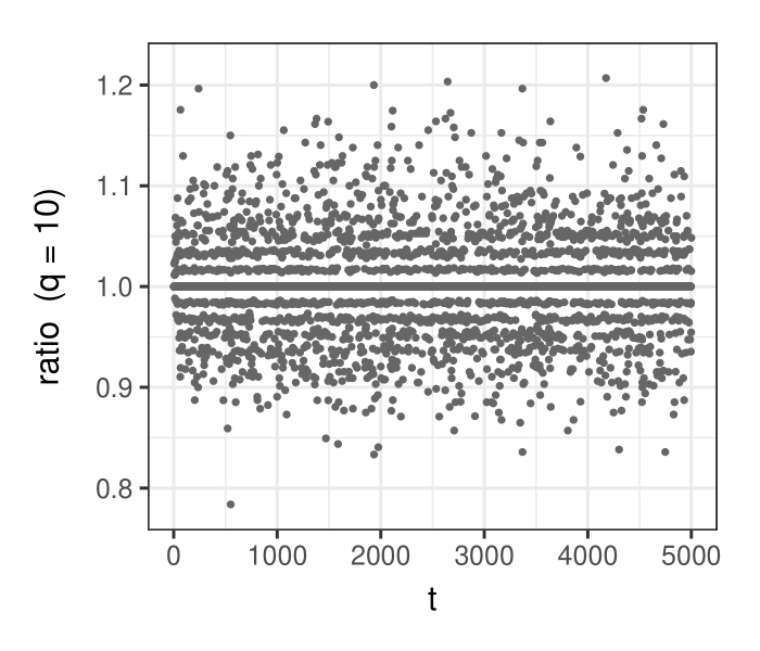
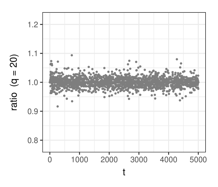
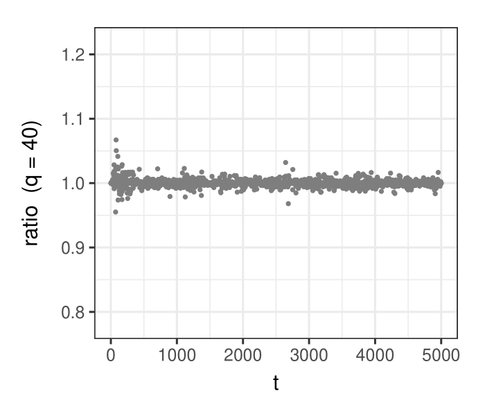
Figure 2: Ratio of proposal distributions $q(\mathcal{D}\,|\,\mathcal{D}^{\prime})/q(\mathcal{D}^{\prime}\,|\,\mathcal{D})$ for a Markov chain on the DAG space $\mathcal{S}_{q}$ generated using Algorithm 2. Each dot is the ratio of proposals for the current DAG $\mathcal{D}$ and its sampled successor $\mathcal{D}^{\prime}$. Left to right-side panels refer to $q\in\{10,20,40\}$ respectively.

4.3 Update of DAG-parameters

In the second step of the MCMC scheme we then sample the model-dependent parameters $(\bm{D},\bm{L})$ conditionally on the accepted DAG $\mathcal{D}$ from their full conditional distribution

$$p(\bm{D},\bm{L}\,|\,\mathcal{D},\bm{X})=\prod_{j=1}^{q}p(\bm{L}_{\prec j\,]}\,|\,\bm{D}_{jj},\mathcal{D},\bm{X})\,p(\bm{D}_{jj}\,|\,\mathcal{D},\bm{X}).$$ (21)

Equation (21) corresponds to the DAG-Wishart posterior distribution in (7). As mentioned, direct sampling from $p(\bm{D},\bm{L}\,|\,\mathcal{D},\bm{X})$ can be performed using the rDAGWishart function introduced in Section 2.3; see also Section 2.4.

4.4 MCMC algorithm

Our main MCMC scheme for posterior inference on DAGs and DAG-parameters is summarized in Algorithm 4.

Input: $S$, $B$, $\bm{X}$, $a,\bm{U},w$

Output: $S$ samples from the posterior distribution (17)

1 Initialize $\mathcal{D}^{(0)}$, e.g. the empty DAG;

2 for $s=1,\dots,B+S$ do

3       Sample $\mathcal{D}^{\prime}$ from $q(\mathcal{D}^{\prime}\,|\,\mathcal{D}^{(s-1)})$ using Algorithm 2 or its fast version (Algorithm 3);

4       Set $\mathcal{D}^{(s)}=\mathcal{D}^{\prime}$ with probability $\alpha_{\mathcal{D}^{\prime}}=\min\{1;r_{\mathcal{D}^{\prime}}\}$ in (20), otherwise $\mathcal{D}^{(s)}=\mathcal{D}^{(s-1)}$;

5       Sample $\big{(}\bm{D}^{(s)},\bm{L}^{(s)}\big{)}$ from its full conditional (21);

6      

7 end for

return $\big{\{}\big{(}\bm{D}^{(s)},\bm{L}^{(s)},\mathcal{D}^{(s)}\big{)},s=B+1,\dots,B+S\big{\}}$

Algorithm 4 MCMC scheme to sample from the posterior of DAGs and parameter

Algorithm 4 is implemented within our package in the function learn_DAG(S, burn, data, a, U, w, fast = FALSE, save.memory = FALSE, collapse = FALSE). Main arguments of the function are:

• S: the number of final MCMC draws from the posterior;

• burn: the burn-in period;

• data: the $(n,q)$ data matrix $\bm{X}$;

• a, U: the hyperparameters of the DAG-Wishart prior;

• w: the prior probability of edge inclusion.

The default setting fast = FALSE implements the MCMC proposal distribution of Algorithm 2 which requires the enumeration of all direct successor DAGs in each local move. By converse, with fast = TRUE the approximate proposal of Algorithm 3 is adopted.

Whenever the interest is on DAG structure learning only, rather than on both DAG learning and parameter inference, a collapsed MCMC sampler can be considered. In such a case, the target distribution is represented by the marginal posterior over the DAG space

$$p(\mathcal{D}\,|\,\bm{X})\propto m(\bm{X}\,|\,\mathcal{D})\,p(\mathcal{D}),$$ (22)

where $m(\bm{X}\,|\,\mathcal{D})$ is the marginal likelihood of DAG $\mathcal{D}$ derived in Section 2.5. An MCMC sampler targeting the posterior $p(\mathcal{D}\,|\,\bm{X})$, $\mathcal{D}\in\mathcal{S}_{q}$, can be constructed as in Algorithm 5 and implemented by learn_DAG by setting collapse = TRUE.

Input: $S$, $B$, $\bm{X}$, $a,\bm{U},w$

Output: $S$ samples from the posterior in (17)

1 Initialize $\mathcal{D}^{(0)}$, e.g. the empty DAG;

2 for $s=1,\dots,B+S$ do

3       Sample $\mathcal{D}^{\prime}$ from $q(\mathcal{D}^{\prime}\,|\,\mathcal{D}^{(s-1)})$ using Algorithm 2 or its fast version (Algorithm 3);

4       Set $\mathcal{D}^{(s)}=\mathcal{D}^{\prime}$ with probability $\alpha_{\mathcal{D}^{\prime}}=\min\{1;r_{\mathcal{D}^{\prime}}\}$ in (20), otherwise $\mathcal{D}^{(s)}=\mathcal{D}^{(s-1)}$;

5      

6 end for

return $\big{\{}\mathcal{D}^{(s)},s=B+1,\dots,B+S\big{\}}$

Algorithm 5 Collapsed MCMC scheme to sample from the posterior of DAGs

By default, with save.memory = FALSE, learn_DAG returns a list of $(q,q,S)$-dimensional arrays. However, as the dimension of the chain increases, the user may incur in memory usage restrictions. By setting save.memory = TRUE, at each iteration the sampled matrices are converted into character strings and stored in a vector, thus reducing the size of the output. Function bd_decode also allows to convert the output into the original array format.

4.5 Posterior inference

Algorithm 4 produces a collection of DAGs $\big{\{}\mathcal{D}^{(s)}\big{\}}_{s=1}^{S}$ and DAG-parameters $\big{\{}\big{(}\bm{D}^{(s)},\bm{L}^{(s)}\big{)}\big{\}}_{s=1}^{S}$ visited by the MCMC algorithm which can be used to approximate the target distribution in (17). An approximate posterior distribution over the space $\mathcal{S}_{q}$ can be obtained as

$$\hat{p}(\mathcal{D}\,|\,\bm{X})=\frac{1}{S}\sum_{s=1}^{S}\mathbbm{1}\big{\{}\mathcal{D}^{(s)}=\mathcal{D}\big{\}},$$ (23)

that is through the MCMC frequency of visits of each DAG $\mathcal{D}$. In addition, we can compute, for each $(u,v)$, $u\neq v$, the posterior probability of edge inclusion

$$\hat{p}_{u\rightarrow v}(\bm{X})\equiv\hat{p}_{u\rightarrow v}=\frac{1}{S}\sum_{s=1}^{S}\mathbbm{1}_{u\rightarrow v}\big{\{}\mathcal{D}^{(s)}\big{\}},$$ (24)

where $\mathbbm{1}_{u\rightarrow v}\big{\{}\mathcal{D}^{(s)}\big{\}}$ takes value 1 if and only if $\mathcal{D}^{(s)}$ contains the edge $u\rightarrow v$. A $(q,q)$ matrix collecting the posterior probabilities of edge inclusion can be constructed through the function get_edgeprobs(learnDAG_output) which requires as the only argument the output of learn_DAG.

Single DAG estimates summarizing the MCMC output can be also recovered. For instance, one can consider the Maximum A Posteriori (MAP) DAG estimate, corresponding to the DAG with the highest estimated posterior probability. Alternatively, we can construct the Median Probability (DAG) Model (MPM) which is instead obtained by including all edges $u\rightarrow v$ whose estimated probability of inclusion (24) exceeds 0.5. The two DAG estimates can be constructed through the functions get_MAPdag(learnDAG_output) and get_MPMdag(learnDAG_output) respectively.

Given the MCMC output, we can recover the collection of precision matrices $\big{\{}\bm{\Omega}^{\mathcal{D}^{(s)}}\big{\}}_{s=1}^{S}$ using the relationship $\bm{\Omega}=\bm{L}\bm{D}^{-1}\bm{L}^{\top}$. For a given intervention target $I\subseteq\{1,\dots,q\}$, recall now the definition of causal effect of $X_{h}$ on $Y$ $(h\in I)$ in a joint intervention on $\{X_{j}\}_{j\in I}$ summarized in Section 3. Draws from the posterior distribution of each causal effect coefficient $\theta_{h,Y}^{I}$, $h\in I$, can be then recovered using (16). This is performed by function get_causaleffect(learnDAG_output, targets, response, BMA = FALSE) under the default choice BMA = FALSE. Arguments of the function are:

• learnDAG_output: the output of learn_dag;

• targets: a vector with the numerical labels of the intervened nodes in $I$;

• response: the numerical label of the response variable of interest $Y$.

Its output therefore consists of $S$ draws $\big{\{}\theta_{h,Y}^{I(1)},\dots,\theta_{h,Y}^{I(S)}\big{\}}$ approximately sampled from the posterior of each causal effect coefficient $\theta_{h,Y}^{I}$, $h\in I$. As a summary of the posterior distribution of each $\theta_{h,Y}^{I}$ we can further consider

$$\hat{\theta}_{h,Y}^{I}=\frac{1}{S}\sum_{s=1}^{S}\theta_{h,Y}^{I(s)},$$ (25)

which corresponds to a Bayesian Model Averaging (BMA) estimate wherein posterior model probabilities are approximated through their MCMC frequencies of visits. BMA estimates of causal effect coefficients are returned by get_causaleffects when BMA = TRUE.

4.6 MCMC diagnostics of convergence

MCMC diagnostics of convergence can be performed by monitoring how specific graph features vary across MCMC iterations. Selected diagnostics that we now detail are implemented by function get_diagnostics, which takes as input the MCMC output of learn_DAG.

We start by focusing on the number of edges in the DAG. The first ouput of get_diagnostics is a trace plot of the number of edges in the DAGs visited by the MCMC chain at each step $s=1,...,S$. The absence of trends in the plot generally suggests a good degree of MCMC mixing. In addition, a trace plot of the average number of edges in the DAGs visited up to time $s$, for $s=1,...,S$, is returned. In this case, the convergence of the plot around a “stable” average size represents a symptom of genuine MCMC convergence.

We further monitor the posterior probability of edge inclusion computed, for each edge $u\rightarrow v$, up to time $s$, for $s=1,\dots,S$. Each posterior probability is estimated as the proportion of DAGs visited by the MCMC up to time $s$ which contain the directed edge $u\rightarrow v$; see also Equation (24). Output is organized in $q$ plots (one for each node $v=1,\dots,q$), each summarizing the posterior probabilities of edges $u\rightarrow v$, $u=1,\dots,q$. The stabilization of each posterior probability around a constant level reflects a good degree of MCMC convergence; see also the following section 5 for more detailed illustrations.

5 Illustrations

In this section we exemplify the use of BCDAG through both simulated and real data.

5.1 Simulated data

We first use the function rDAG(q, w) to randomly generate a DAG structure with $q=8$ nodes by fixing a probability of edge inclusion $w=0.2$.

Ψq <- 8
Ψset.seed(123)
ΨDAG <- rDAG(q = q, w = 0.2)
ΨDAG
Ψ1 2 3 4 5 6 7 8
Ψ1 0 0 0 0 0 0 0 0
Ψ2 0 0 0 0 0 0 0 0
Ψ3 0 1 0 0 0 0 0 0
Ψ4 0 0 0 0 0 0 0 0
Ψ5 1 0 0 0 0 0 0 0
Ψ6 1 1 1 1 0 0 0 0
Ψ7 0 0 0 1 1 0 0 0
Ψ8 0 0 0 0 0 0 0 0

Given the so-obtained DAG, above represented through its adjacency matrix DAG, we then generate the non-zero off-diagonal elements of $\bm{L}$ uniformly in the interval $[0.1,1]$, while we fix $\bm{D}=\bm{I}_{q}$.

ΨL <- matrix(runif(n = q*(q-1), min = 0.1, max = 1), q, q)*DAG; diag(L) <- 1
ΨD <- diag(1, q)

Finally, we generate $n=200$ multivariate zero-mean Gaussian data as in (1), by recovering first the precision matrix $\bm{\Omega}=\bm{L}\bm{D}^{-1}\bm{L}^{\top}$ and then using the function rmvnorm within the package mvtnorm:

ΨOmega <- L%*%solve(D)%*%t(L)
ΨX <- mvtnorm::rmvnorm(n = 200, sigma = solve(Omega))

We run function learn_DAG to approximate the posterior over DAGs and DAG-parameters (collapse = FALSE) by fixing the number of final MCMC iterations and burn-in period as $S=5000$, $B=1000$, while prior hyperparameters as $a=q,\bm{U}=\bm{I}_{q},w=0.1$. We implement the approximate MCMC proposal (Section 4.2) by setting fast = TRUE:

Ψout_mcmc <- learn_DAG(S = 5000, burn = 1000, data = X, a = q, U = diag(1,q),
Ψ            w = 0.1, fast = TRUE, save.memory = FALSE, collapse = FALSE)

out_mcmc, the output of function learn_DAG, corresponds to a list with three elements:

• out_mcmc$graphs: a $(q,q,S)$ array with the adjacency matrices of DAGs $\mathcal{D}^{(1)},\dots,$ $\mathcal{D}^{(S)}$ sampled by the MCMC;

• out_mcmc$L: a $(q,q,S)$ array with the $S$ matrices $\bm{L}^{(1)},\dots,\bm{L}^{(S)}$ sampled by the MCMC;

• out_mcmc$D: a $(q,q,S)$ array with the $S$ matrices $\bm{D}^{(1)},\dots,\bm{D}^{(S)}$ sampled by the MCMC.

Given the MCMC output, we can compute the posterior probabilities of edge inclusion using function get_edgeprobs. The latter returns a $(q,q)$ matrix with $(u,v)$-element corresponding to the estimated posterior probability $\hat{p}_{u\rightarrow v}$ in Equation (24). In addition, the MAP and MPM DAG estimates can be recovered through get_MAPdag and get_MPMdag respectively:

Ψget_edgeprobs(learnDAG_output = out_mcmc)
Ψ
Ψ
Ψ       1      2      3      4      5      6      7      8
Ψ1 0.0000 0.0000 0.0072 0.0012 0.0000 0.0000 0.0066 0.0038
Ψ2 0.0000 0.0000 0.1084 0.0084 0.0352 0.9182 0.0000 0.0258
Ψ3 0.0280 0.0504 0.0000 0.0828 0.0000 0.8872 0.0068 0.1822
Ψ4 0.0008 0.0000 0.0126 0.0000 0.0136 0.0174 0.0292 0.0158
Ψ5 1.0000 0.0082 0.0000 0.0028 0.0000 0.0000 0.4344 0.1360
Ψ6 1.0000 0.0558 0.1128 0.9826 0.0000 0.0000 0.0330 0.0110
Ψ7 0.0006 0.0044 0.0326 0.9708 0.5656 0.0214 0.0000 0.0360
Ψ8 0.0154 0.0206 0.0666 0.0142 0.1056 0.0036 0.0136 0.0000

Ψget_MAPdag(learnDAG_output = out_mcmc)
Ψ
Ψ  1 2 3 4 5 6 7 8
Ψ1 0 0 0 0 0 0 0 0
Ψ2 0 0 0 0 0 1 0 0
Ψ3 0 0 0 0 0 1 0 0
Ψ4 0 0 0 0 0 0 0 0
Ψ5 1 0 0 0 0 0 0 0
Ψ6 1 0 0 1 0 0 0 0
Ψ7 0 0 0 1 1 0 0 0
Ψ8 0 0 0 0 0 0 0 0

Ψ
Ψget_MPMdag(learnDAG_output = out_mcmc)
Ψ
Ψ  1 2 3 4 5 6 7 8
Ψ1 0 0 0 0 0 0 0 0
Ψ2 0 0 0 0 0 1 0 0
Ψ3 0 0 0 0 0 1 0 0
Ψ4 0 0 0 0 0 0 0 0
Ψ5 1 0 0 0 0 0 0 0
Ψ6 1 0 0 1 0 0 0 0
Ψ7 0 0 0 1 1 0 0 0
Ψ8 0 0 0 0 0 0 0 0

Suppose now we are interested in evaluating the total causal effect on node $Y=X_{1}$ consequent to a joint intervention on variables in $I=\{5,6,7\}$. An approximate posterior distribution for the vector parameter $\big{(}\theta^{I}_{h,Y}\big{)}_{h\in I}$ representing the total causal effect (Section 3) can be recovered from the MCMC output as

Ψjoint_causal <- get_causaleffect(learnDAG_output = out_mcmc,
Ψ                targets = c(5,6,7), response = 1, BMA = FALSE)
Ψ
Ψhead(joint_causal)
Ψ
Ψ          h = 5      h = 6 h = 7
Ψ[1,] -0.6323857 -0.7955013     0
Ψ[2,] -0.5649460 -0.8802489     0
Ψ[3,] -0.5961280 -0.8219784     0
Ψ[4,] -0.5790337 -0.8392289     0
Ψ[5,] -0.6657683 -0.8439536     0
Ψ[6,] -0.6334429 -0.9030620     0

joint_causal thus consists of a $(S,3)$ matrix, with each column referring to one of the three intervened variables. The posterior distribution of each causal effect coefficient $\theta_{h,Y}^{I}$, $h\in I$, is summarized in the box-plots of Figure 3.

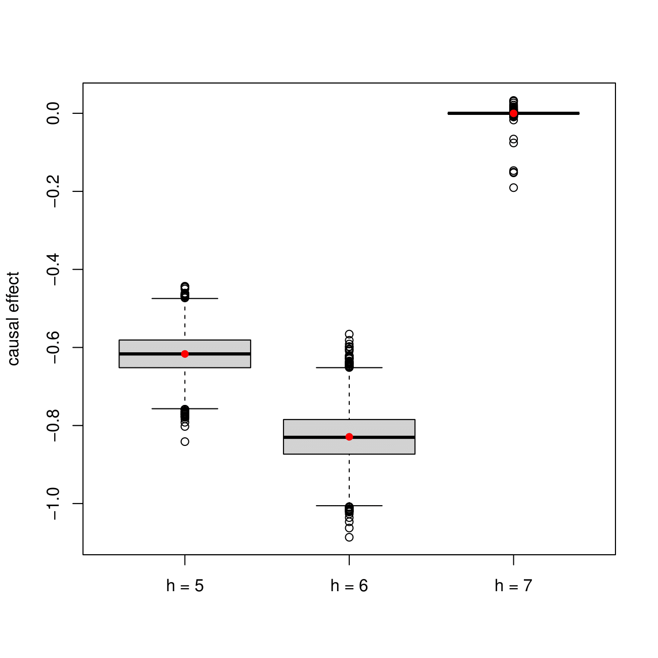
Figure 3: Simulated data. Posterior distribution of the causal effect coefficient $\theta^{I}_{h,1}$ for $h\in I$ and target of intervention $I=\{5,6,7\}$. BMA estimates are represented as red dots.

By setting BMA = TRUE, a Bayesian Model Averaging (BMA) estimate of the three parameters is returned. Each BMA estimate is obtained as the sample mean of the corresponding posterior draws in joint_causal; see also Equation (25).

Ψout_causal_BMA <- get_causaleffect(learnDAG_output = out_mcmc,
Ψ                  targets = c(5,6,7), response = 1, BMA = TRUE)
Ψ
Ψround(out_causal_BMA, 4)
Ψ
Ψ  h = 5   h = 6   h = 7
Ψ-0.6167 -0.8290 -0.0001

5.2 Real data analyses

In this section we consider a biological dataset of patients affected by Acute Myeloid Leukemia (AML). The dataset contains the levels of $q=18$ proteins and phosphoproteins involved in apoptosis and cell cycle regulation according to the KEGG database (Kanehisa et al., 2012) and is provided as a supplement of Kornblau et al. (2009). Measurements relative to $256$ newly diagnosed AML patients are included in the original dataset. In addition, subjects are classified according to the French-American-British (FAB) system into several different AML subtypes. The same dataset was analyzed by Peterson et al. (2015) and Castelletti et al. (2020) from a multiple graphical model perspective to estimate group-specific dependence structures based on undirected and directed graphs respectively.

In the sequel we focus on subtype M2 and consider the $n=68$ corresponding observations which are collected in leukemia_data.csv. We run the MCMC scheme in Algorithm 4 and implemented by learn_DAG by fixing $S=60000,B=5000,a=q,\bm{U}=\frac{1}{n}\bm{I}_{q}$, $w=0.5$:

ΨX <- read.csv("leukemia_data.csv", sep = ",")
Ψq <- ncol(X); n <- nrow(X)
Ψout_mcmc <- learn_DAG(S = 60000, burn = 5000, data = X, a = q,
Ψ            U = diag(1,q)/n, w = 0.5, fast = TRUE, collapse = FALSE)

We first perform MCMC diagnostics of convergence (Section 4.6) by running:

Ψget_diagnostics(learnDAG_output = out_mcmc)

We report in the left-side panel of Figure 4 the trace plot of the number of edges in the graphs visited by the MCMC at each iteration $s=1,\dots,S$. The right-side panel of the same figure instead reports the trace plot of the average number of edges in the DAGs visited by the MCMC up to iteration $s$, for $s=1,\dots,S$. The apparent absence of trends in the trace plot and the curve stabilization around an average value both suggest a good degree of MCMC mixing and convergence to the target distribution.

Figure 5 summarizes the behaviour of the posterior probabilities of inclusion of selected edges across MCMC iterations. Specifically, each plot refers to one node $v\in\{13,\dots,18\}$ and contains a collection of trace plots each representing the posterior probability of inclusion of $u\rightarrow v$, ($u\neq v$) computed up to iteration $s$, for $s=1,\dots,S$. By inspection, we can appreciate the convergence of each curve around stable values.

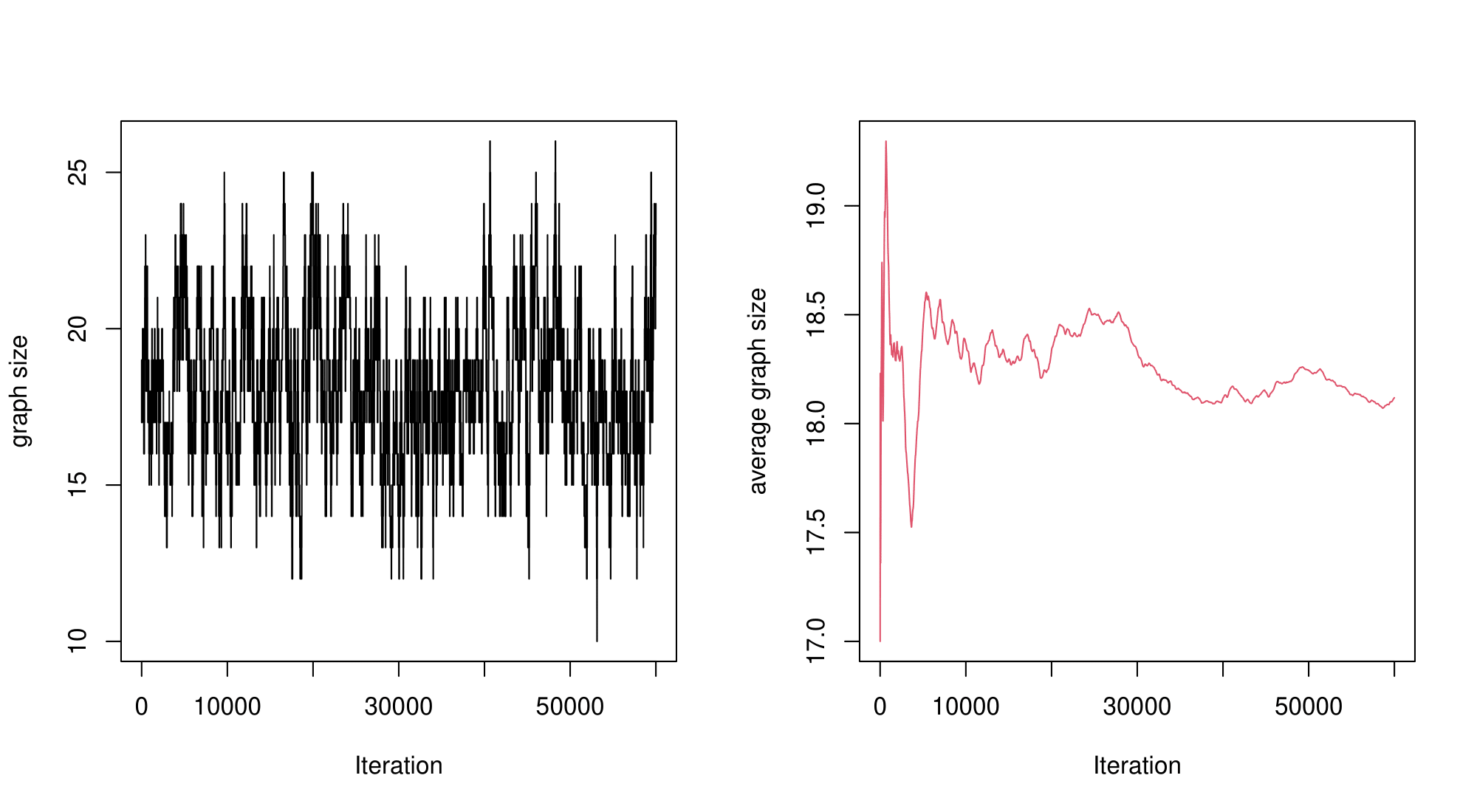
Figure 4: Leukemia data. Trace plot of the number of edges (graph size) in the DAGs visited by the MCMC at each iteration (left panel). Trace plot of the average number of edges in the DAGs computed up to iteration $s$, $s=1,\dots,60000$ (right panel).

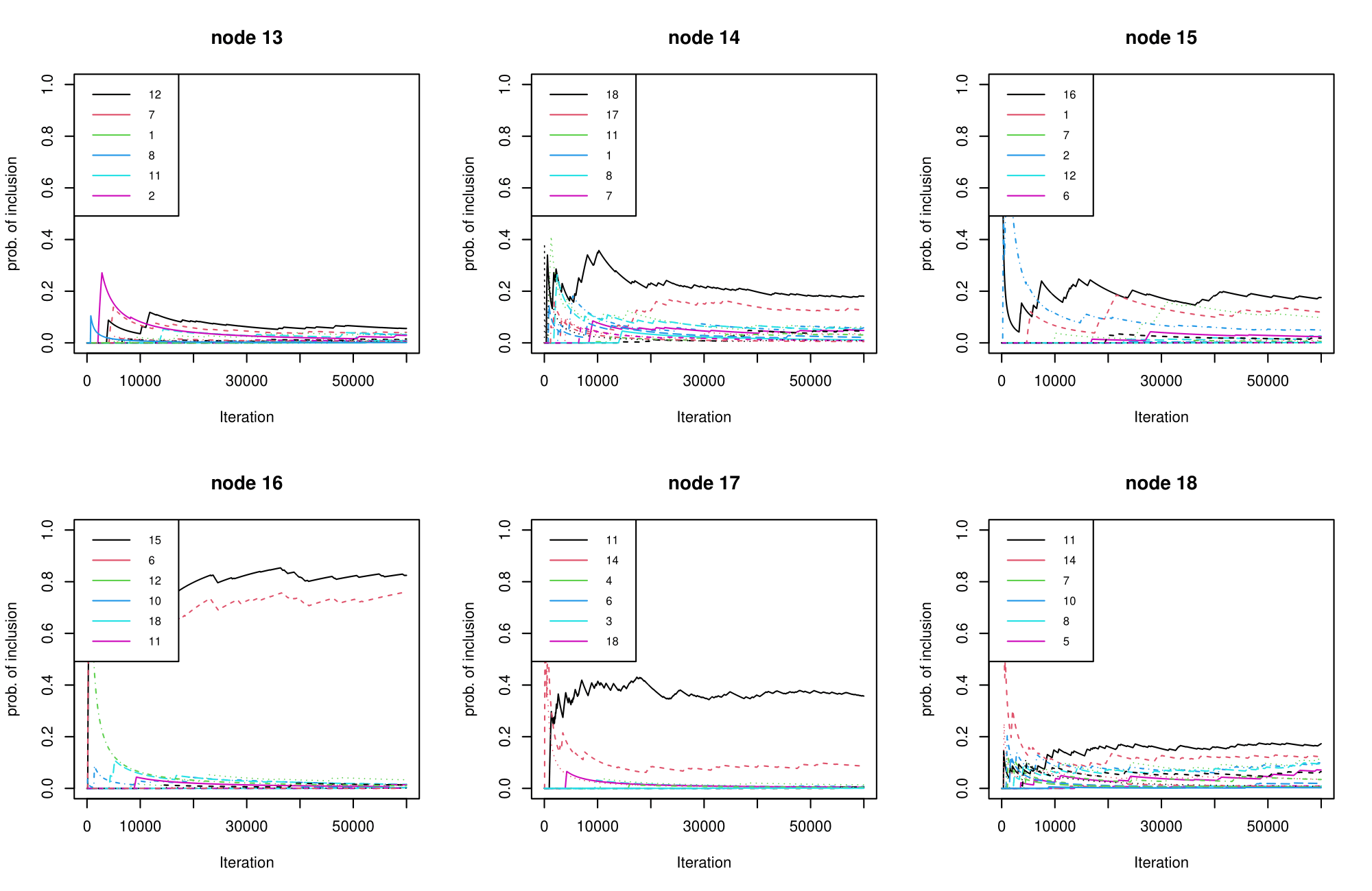
Figure 5: Leukemia data. Trace plot of the posterior probability of inclusion of $u\rightarrow v$, computed across iteration $s$, for selected nodes $v\in\{13,\dots,18\}$. For each node $v$, the six nodes $u$ associated with the highest posterior probabilities $p_{u\rightarrow v}$ are reported in the legend.

Given the MCMC output, we now proceed by constructing posterior summaries of interest. Specifically, we first recover the posterior probabilities of inclusion $\hat{p}_{u\rightarrow v}$ in Equation 24 for each $u\rightarrow v$, $u\neq v$. These are collected in the $(q,q)$ matrix returned by get_edgeprobs which is obtained as follows:

Ψpost_edge_probs <- get_edgeprobs(learnDAG_output = out_mcmc)

In Figure 5 we represent the resulting matrix post_edge_probs as a heat-map, with a dot at position $(u,v)$ corresponding to the estimated probability $\hat{p}_{u\rightarrow v}$. In addition, we recover the Median Probability DAG-Model (MPM) as:

ΨMPM_dag <- get_MPMdag(out_mcmc)

Object MPM_dag corresponds to the adjacency matrix of the resulting graph estimate, which is represented in Figure 7.

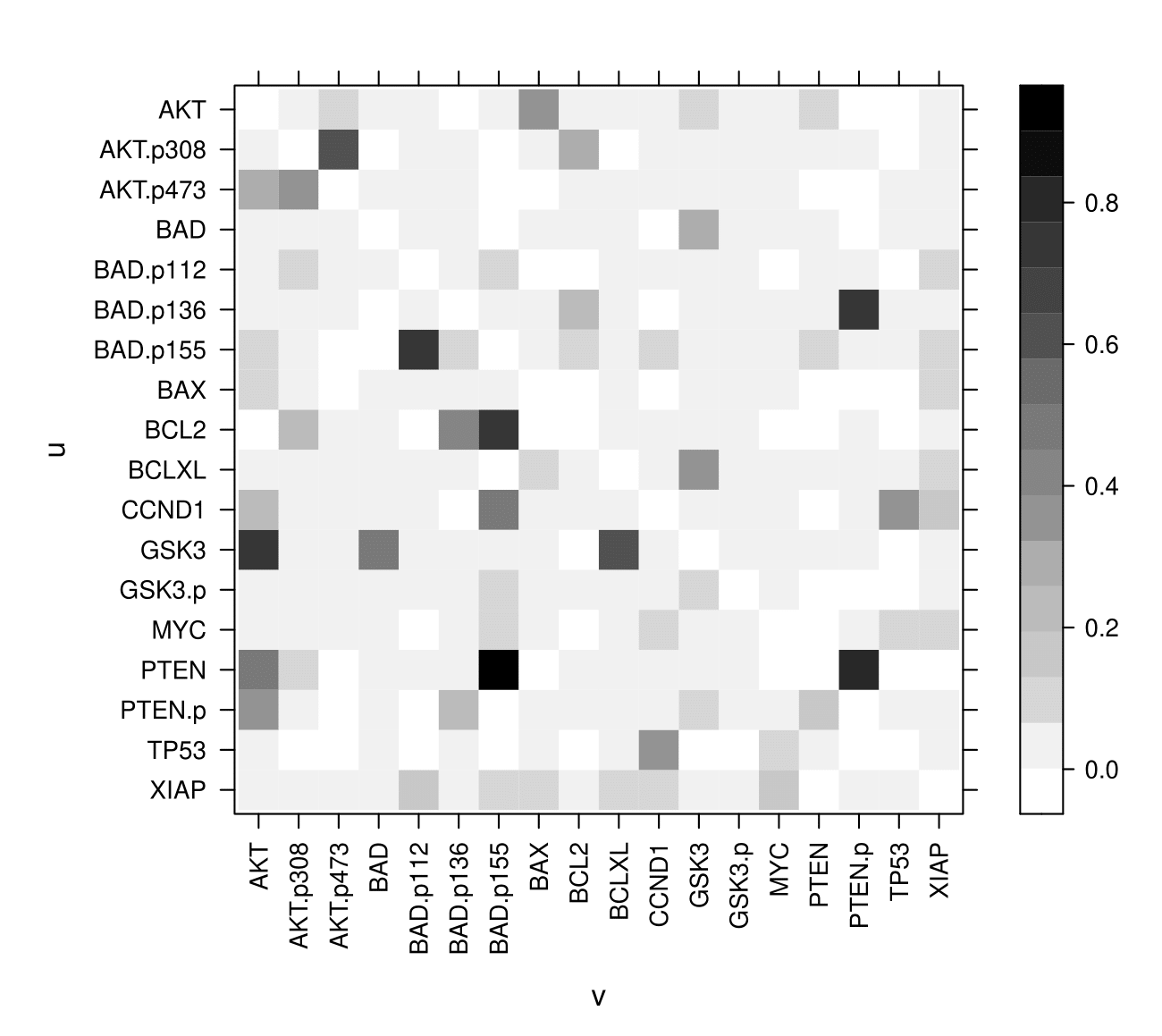
Figure 6: Leukemia data. Heat map with posterior probabilities of edge inclusion, for each directed edge $u\rightarrow v$.

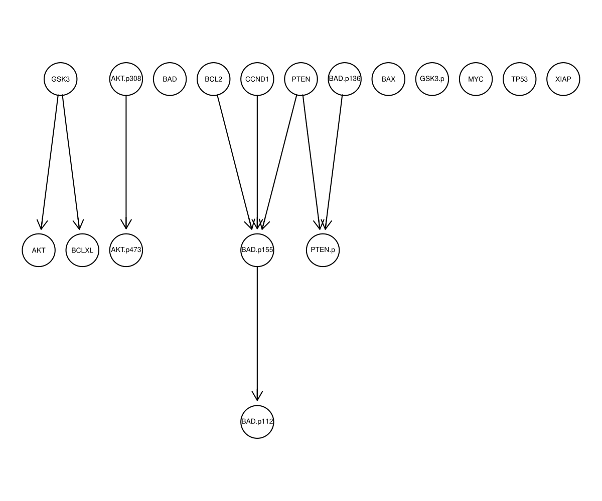
Figure 7: Leukemia data. Median Probability DAG-Model (MPM) estimate.

We now focus on causal effect estimation. Among the proteins included in the study, AKT has received particular interest because of its role played in leukemogenesis. Specifically, AKT belongs to the PI3K-Akt-mTOR pathway, which is one of the intracellular pathways aberrantly up-regulated in AML; see also Nepstad et al. (2020). Because of its role played in AML progression, we then consider the AKT protein as the response of interest for our causal-effect analysis.

We first evaluate the causal effect of a single-node $(I=j)$ intervention $\text{do}\{X_{j}=\tilde{x}_{j}\}$ on $Y$ for each $j\in\{1,\dots,q\}$. The resulting collection of coefficients can provide useful information on the effect of selected interventions on each protein w.r.t. AKT. In particular, this can help identifying promising targets for AKT regulation. Results, in terms of posterior distributions of coefficients $\theta_{j,Y}^{j}$, for $j=1,\dots,q$, are obtained by running

Ψcausal_all <- sapply(1:q, function(h) get_causaleffect(out_mcmc,
Ψ              targets = j, response = 1, BMA = FALSE))

and are summarized in the box-plots of Figure 8.

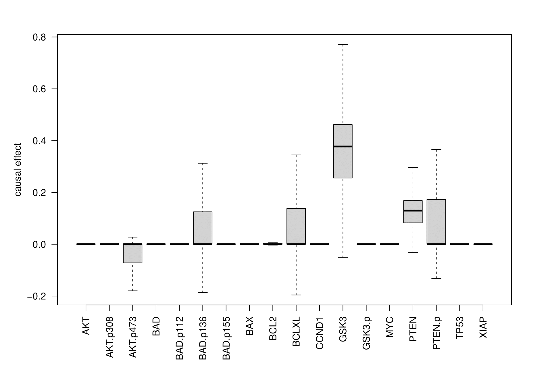
Figure 8: Leukemia data. Posterior distribution of the causal effect coefficient of an intervention $\text{do}\{X_{j}=\tilde{x}_{j}\}$ on response $Y=\textnormal{AKT}$, for $j\in\{1,\dots,q\}$ (each node labelled with the corresponding protein name).

As a further example, consider a joint intervention acting on the GSK3 protein and phosphoprotein (GSK3 and GSK3.p respectively, corresponding to variables/columns 12 and 13 in the original data matrix X). We evaluate the causal effect of such an intervention w.r.t. AKT, by computing the BMA estimates of the two causal effect coefficients:

Ψcausal_out_12_13 <- get_causaleffect(learnDAG_output = out_mcmc,
Ψ                    targets = c(12,13), response = 1, BMA = F)
Ψround(causal_out_12_13, 4)
Ψh = 12 h = 13
Ψ0.3122 0.0050

6 Conclusions

In this article we introduced BCDAG, a novel R package for Bayesian structure learning and causal effect estimation from Gaussian, observational data. This package implements the method of Castelletti & Mascaro (2021) through a variety of functions that allow for DAG-model selection, posterior inference of model parameters and estimation of causal effects. The proposed implementation scales efficiently to an arbitrarily large number of observations and, whenever the visited DAGs are sufficiently sparse, to datasets with a large number of variables. However, convergence of MCMC algorithms in high dimensional (large $q$) settings can be extremely slow, thus hindering posterior inference. For this reason, we plan to extend the proposed method by considering alternative MCMC schemes that may improve convergence to the target posterior distribution; see for instance Kuipers et al. (2021) and Agrawal et al. (2018). In addition, we are considering extensions of the proposed structure learning method to more general settings where a combination of observational and interventional (experimental) data is available (Castelletti & Consonni, 2019).

We finally encourage R users to provide feedback, questions or suggestion by e-mail correspondence or directly through our github code repository https://github.com/alesmascaro/BCDAG.

References

- Agrawal et al. (2018) Agrawal, R., Uhler, C. & Broderick, T. (2018). Minimal i-MAP MCMC for scalable structure discovery in causal DAG models. In J. Dy & A. Krause, eds., Proceedings of the 35th International Conference on Machine Learning, vol. 80. 89–98.
- Andersson et al. (1997) Andersson, S. A., Madigan, D. & Perlman, M. D. (1997). A characterization of Markov equivalence classes for acyclic digraphs. The Annals of Statistics 25 505–541.
- Ben-David et al. (2015) Ben-David, E., Li, T., Massam, H. & Rajaratnam, B. (2015). High dimensional Bayesian inference for Gaussian directed acyclic graph models. arXiv pre-print .
- Cao et al. (2019) Cao, X., Khare, K. & Ghosh, M. (2019). Posterior graph selection and estimation consistency for high-dimensional Bayesian DAG models. The Annals of Statistics 47 319–348.
- Castelletti & Consonni (2019) Castelletti, F. & Consonni, G. (2019). Objective Bayes model selection of Gaussian interventional essential graphs for the identification of signaling pathways. The Annals of Applied Statistics 13 2289–2311.
- Castelletti & Consonni (2021a) Castelletti, F. & Consonni, G. (2021a). Bayesian causal inference in probit graphical models. Bayesian Analysis 16 1113–1137.
- Castelletti & Consonni (2021b) Castelletti, F. & Consonni, G. (2021b). Bayesian inference of causal effects from observational data in Gaussian graphical models. Biometrics 77 136–149.
- Castelletti et al. (2018) Castelletti, F., Consonni, G., Vedova, M. L. D. & Peluso, S. (2018). Learning Markov equivalence classes of directed acyclic graphs: An objective Bayes approach. Bayesian Analysis 13 1235–1260.
- Castelletti et al. (2020) Castelletti, F., La Rocca, L., Peluso, S., Stingo, F. C. & Consonni, G. (2020). Bayesian learning of multiple directed networks from observational data. Statistics in Medicine 39 4745–4766.
- Castelletti & Mascaro (2021) Castelletti, F. & Mascaro, A. (2021). Structural learning and estimation of joint causal effects among network-dependent variables. Statistical Methods & Applications 30 1289–1314.
- Chickering (2002) Chickering, D. M. (2002). Optimal structure identification with greedy search. Journal of Machine Learning research 3 507–554.
- Cooper & Herskovits (1992) Cooper, G. F. & Herskovits, E. (1992). A Bayesian method for the induction of probabilistic networks from data. Machine Learning 9 309–347.
- Geiger & Heckerman (2002) Geiger, D. & Heckerman, D. (2002). Parameter priors for directed acyclic graphical models and the characterization of several probability distributions. The Annals of Statistics 30 1412–1440.
- Glymour et al. (1988) Glymour, C., Scheines, R., Spirtes, P. & Kelly, K. (1988). Tetrad: Discovering causal structure. Multivariate Behavioral Research 23 279–280.
- Godsill (2012) Godsill, S. J. (2012). On the relationship between Markov chain Monte Carlo methods for model uncertainty. Journal of Computational and Graphical Statistics 10 230–248.
- Harris & Drton (2013) Harris, N. & Drton, M. (2013). PC algorithm for nonparanormal graphical models. Journal of Machine Learning Research 14 3365–3383.
- Hauser & Bühlmann (2012) Hauser, A. & Bühlmann, P. (2012). Characterization and greedy learning of interventional Markov equivalence classes of directed acyclic graphs. Journal of Machine Learning Research 13 2409–2464.
- Heckerman et al. (1995) Heckerman, D., Geiger, D. & Chickering, D. M. (1995). Learning Bayesian networks: The combination of knowledge and statistical data. Machine Learning 20 197–243.
- Heinze-Deml et al. (2018a) Heinze-Deml, C., Maathuis, M. H. & Meinshausen, N. (2018a). Causal structure learning. Annual Review of Statistics and Its Application 5 371–391.
- Heinze-Deml et al. (2018b) Heinze-Deml, C., Peters, J. & Meinshausen, N. (2018b). Invariant causal prediction for nonlinear models. Journal of Causal Inference 6 20170016.
- Kalainathan & Goudet (2019) Kalainathan, D. & Goudet, O. (2019). Causal discovery toolbox: Uncover causal relationships in Python.
- Kalisch et al. (2012) Kalisch, M., Mächler, M., Colombo, D., Maathuis, M. H. & Bühlmann, P. (2012). Causal inference using graphical models with the R package pcalg. Journal of Statistical Software 47 1–26.
- Kanehisa et al. (2012) Kanehisa, M., Goto, S., Sato, Y., Furumichi, M. & Tanabe, M. (2012). KEGG for integration and interpretation of large-scale molecular data sets. Nucleic Acids Research D109–D114.
- Kornblau et al. (2009) Kornblau, S., Tibes, R., Qiu, Y., Chen, W., Kantarjian, H., Andreeff, M., Coombes, K. & Mills, G. (2009). Functional proteomic profiling of AML predicts response and survival. Blood 1 154–164.
- Kuipers et al. (2021) Kuipers, J., Suter, P. & Moffa, G. (2021). Efficient sampling and structure learning of Bayesian networks. arXiv pre-print .
- Lauritzen (1996) Lauritzen, S. L. (1996). Graphical Models. Oxford University Press.
- Maathuis & Nandy (2016) Maathuis, M. & Nandy, P. (2016). A review of some recent advances in causal inference. In P. Bühlmann, P. Drineas, M. Kane & M. van der Laan, eds., Handbook of Big Data. Chapman and Hall/CRC, 387–408.
- Maathuis et al. (2009) Maathuis, M. H., Kalisch, M. & Bühlmann, P. (2009). Estimating high-dimensional intervention effects from observational data. The Annals of Statistics 37 3133–3164.
- Nandy et al. (2017) Nandy, P., Maathuis, M. H. & Richardson, T. S. (2017). Estimating the effect of joint interventions from observational data in sparse high-dimensional settings. The Annals of Statistics 45 647–674.
- Nepstad et al. (2020) Nepstad, I., Hatfield, K., Grønningsæter, I. & Reikvam, H. (2020). The PI3K-Akt-mTOR signaling pathway in human acute myeloid leukemia (AML) cells. International Journal of Molecular Sciences 21.
- Ni et al. (2017) Ni, Y., Stingo, F. C. & Baladandayuthapani, V. (2017). Sparse multi-dimensional graphical models: A unified Bayesian framework. Journal of the American Statistical Association 112 779–793.
- Pearl (2000) Pearl, J. (2000). Causality: Models, Reasoning, and Inference. Cambridge University Press, Cambridge.
- Peluso & Consonni (2020) Peluso, S. & Consonni, G. (2020). Compatible priors for model selection of high-dimensional Gaussian DAGs. Electronic Journal of Statistics 14 4110 – 4132.
- Peters et al. (2017) Peters, J., Janzing, D. & Schölkopf, B. (2017). Elements of Causal Inference: Foundations and Learning Algorithms. The MIT Press.
- Peterson et al. (2015) Peterson, C., Stingo, F. C. & Vannucci, M. (2015). Bayesian inference of multiple Gaussian graphical models. Journal of the American Statistical Association 110 159–174.
- R Core Team (2021) R Core Team (2021). R: A Language and Environment for Statistical Computing. R Foundation for Statistical Computing, Vienna, Austria.
- Russell & Norvig (2009) Russell, S. & Norvig, P. (2009). Artificial Intelligence: A Modern Approach. USA: Prentice Hall Press.
- Scutari (2010) Scutari, M. (2010). Learning Bayesian networks with the bnlearn R package. Journal of Statistical Software 35 1–22.
- Shimizu et al. (2006) Shimizu, S., Hoyer, P. O., Hyvärinen, A., Kerminen, A. & Jordan, M. (2006). A linear non-Gaussian acyclic model for causal discovery. Journal of Machine Learning Research 7 2003–2030.
- Solus et al. (2021) Solus, L., Wang, Y. & Uhler, C. (2021). Consistency guarantees for greedy permutation-based causal inference algorithms. Biometrika 108 795–814.
- Spirtes et al. (2000) Spirtes, P., Glymour, C. & Scheines, R. (2000). Causation, Prediction and Search (2nd edition). Cambridge, MA: The MIT Press.
- Squires & Uhler (2018) Squires, C. & Uhler, C. (2018). CausalDAG: Python package for the creation, manipulation and learning of causal DAGs.
- Suter et al. (2021) Suter, P., Kuipers, J., Moffa, G. & Beerenwinkel, N. (2021). Bayesian structure learning and sampling of Bayesian networks with the R package BiDAG.
- Tsamardinos et al. (2006) Tsamardinos, I., Brown, L. E. & Aliferis, C. F. (2006). The max-min hill-climbing Bayesian network structure learning algorithm. Machine Learning 65 31–78.
- Zhang et al. (2022) Zhang, K., Ramsey, J., Gong, M., Cai, R., Shimizu, S., Spirtes, P. & Glymour, C. (2022). Causal-learn: Causal discovery for Python.