A Universal Machine Learning Model for Elemental Grain Boundary Energies

Abstract

The grain boundary (GB) energy has a profound influence on the grain growth and properties of polycrystalline metals. Here, we show that the energy of a GB, normalized by the bulk cohesive energy, can be described purely by four geometric features. By machine learning on a large computed database of 361 small $\Sigma$ ($\Sigma<10$) GBs of more than 50 metals, we develop a model that can predict the grain boundary energies to within a mean absolute error of 0.13 J m^-2  . More importantly, this universal GB energy model can be extrapolated to the energies of high $\Sigma$ GBs without loss in accuracy. These results highlight the importance of capturing fundamental scaling physics and domain knowledge in the design of interpretable, extrapolatable machine learning models for materials science.

Grain boundaries (GBs) play an important role in determining the strength, toughness, and corrosion resistance of materials[1, 2]. A key property of a GB is its energy, which determines grain growth and the GB distribution. While the GB energy can be accurately calculated using electronic structure methods such as density functional theory (DFT) calculations, the requirement for large supercells to model the inherently low symmetry GB structure limits such computationally intensive approaches to relatively small $\Sigma$ GBs. Nevertheless, substantial databases of GB energies and other properties have been developed using high-throughput DFT. For example, the GB database (GBDB)[3] developed by the present authors contains the calculated GB energies and work of separation of more than 50 elemental metals for both tilt and twist GBs up to $\Sigma=9$.

Alternatively, machine learning (ML) techniques have emerged as a means to develop models that can directly predict the GB energy from compositional and structural features.[4, 5, 6, 7, 8] However, existing ML models targeting elemental GBs are limited in scope by chemistry or structure type, such as face-centered cubic (fcc) Cu [4], Ni [5, 6], Al [7], or body-centered cubic (bcc) Fe [8] systems. These limitations are primarily a result of the choice of data source; these prior works have been developed using data sets computed using embedded atom method (EAM) potentials. While much less computationally intensive than DFT methods, EAM calculations are far less accurate, especially for non-fcc metals,[3] and EAM potentials are available for only a limited subset of elements. Furthermore, the majority of these prior works rely on featurization approaches such as the Smooth Overlap of Atomic Positions (SOAP)[5], [6] and the pair-correlation function (PCF)[7] that generate a large number of features which do not provide direct interpretability using commonly-used GB descriptions.

In this letter, we outline a physics-informed approach to develop a universal ML model for the GB energy of all metals, rather than for a subset of metals. We will demonstrate that the energy of small $\Sigma$ GBs of metals can be predicted to within a mean absolute error (MAE) of 0.13 J m^-2  using a gradient boosting regression (GBR)[9] model of the cohesive energy and four geometric GB features only. More critically, the same model can be extrapolated, without retraining, to predict the energies of high $\Sigma$ GBs with a comparable MAE of 0.12 J m^-2  . This work provides not only a means to rapidly predict the GB energies of any element, but also highlights the importance of choosing appropriate target normalization and features for the development of interpretable and extrapolatable ML.

The critical starting point is in re-evaluating the choice of target for our ML GB model. While prior works have attempted to directly predict the absolute GB energy, we do not believe this to be an optimal choice of target. The GB energy $E_{GB}$ is the excess energy of the GB compared to the bulk per unit area, which can be obtained from computational models as:

$$E_{GB}=\frac{E_{GB,supercell}-n\cdot E^{atom}_{bulk}}{2A}$$ (1)

where $E_{GB,supercell}$ is the energy of the supercell GB model, $n$ is the number of atoms in the GB model, $E^{atom}_{bulk}$ is the energy per atom of the bulk, $A$ is the area of the GB and the factor of 2 accounts for the fact that there are two GBs per supercell model. The physical interpretation is that $E_{GB}$ is related to the energy necessary to break or stretch bonds at the GB from their bulk equilibrium configuration. This energy to stretch or break bonds scales with the cohesive energy of the metal $E_{coh}$ (see Figure LABEL:fig:ecoh),[10] which ranges from $\sim 1.1$ eV atom^-1 for the alkali metals to $\sim 8.9$ eV atom^-1 for tungsten. To remove this chemical scaling effect, we have elected to use the normalized GB energy $\hat{E_{GB}}=E_{GB}/E_{coh}$ as our choice of target.

Based on the coincident-site-lattice (CSL) theory [11, 12], the GB can be specified at a macroscopic level by five degrees of freedom (DOF): two DOFs to define the plane normal of the GB (or alternatively the Miller indices $(hkl)$), two DOFs to define the rotation axis ($[uvw]$) and one DOF to define the misorientation angle ($\theta$). Miller indices, which are defined to be integers by convention, are non-optimal for a regression task. As such, the $(hkl)$ and $[uvw]$ were converted to the inter-planar distances of the GB plane ($d_{GB}$) and the normal plane to the rotation axis ($d_{rot}$), respectively. The cosine of the misorientation angle ($\cos\theta$) was used instead of the misorientation angle itself.

In addition to these geometric GB features, we included three additional features related to bond stretching and breaking at the GB, which were partially inspired by prior works in the literature[13]. To describe the bond deformation, we used both the average bond length in the GB supercell, $\bar{BL}=\sum_{i=1}^{n}(BL_{GB}^{i})/n$, and the average change in bond lengths between the GB supercell and its bulk conventional lattice, $\bar{\Delta BL}=\sum_{i=1}^{n}(BL_{GB}^{i}-BL_{0})/n$, where $BL_{GB}^{i}$ is the bond length of the $i$th bond in the GB supercell, $BL_{0}$ is the bond length in the corresponding bulk conventional structure, and $n$ is the number of bonds counted in the GB supercell. Here, the bonds are identified by performing a local environment analysis via a Voronoi tessellation-based algorithm implemented in the Python Materials Genomics (pymatgen) package[14]. A positive (negative) $\bar{\Delta BL}$ indicates overall bond stretching (compressing) at the GB. According to the Read-Shockley dislocation model[15], $E_{GB}$ of GBs with small misorientation angles is proportional to the shear modulus $G$. Ratanaphan et al.[10] have also shown previously that the GB energies of bcc Mo and Fe are related to $G$. The multi-linear regression models developed by Zheng et al. [3] extended this conclusion to more bcc, fcc, and hexagonal closest packed (hcp) metals. Therefore, we include the DFT Voigt-Reuss-Hill shear modulus $G$ from the Materials Project as the final feature. Figure 1(a) summarizes the preliminary set of six features considered in work.

An initial dataset of GB energies was obtained from the GBDB[3], which contains the energies of 316 GBs of 53 elements in fcc, bcc, hcp and double-hcp (dhcp) structures, after excluding Lu, Eu, and Hg due to the lack of the bulk elastic data. The $\Sigma$s of the GBs range from 3 to 9. The maximum Miller index (MMI) for the rotation axis and the grain boundary plane are 1 and 3, respectively. In this work, we extended the MMI for the grain boundary plane to 4 for 5 elements (As, Nb, Pt, Cu, and Ir), which added 5 more GBs to the initial data. Interested readers are referred to ref 3 for the details on the GB structure generation and computational methods. For the model development, the 321 GBs with $\Sigma\leq 9$ were divided into training (258 GBs) and test (63 GBs) sets using stratified random sampling. The training data comprises 80% of the GBs from each element with more than one GB, and the single GB from the remaining elements.

A preliminary model selection process was performed in an automatic fashion utilizing a tree-based pipeline optimization tool (TPOT)[16] with the six initial features (refer to Supplementary Materials for details). The suggested pipeline from TPOT is a decision-tree-based GBR model preceded by a polynomial feature transformation step. We recognize that there is a risk of redundancy in our selected features, e.g., $G$ has a direct relationship with $E_{coh}$, which was used to normalize the GB energy. Therefore, a comprehensive search for the “best subset” of the six initial features was performed using the suggested pipeline. As shown in Figure 1(b), it was found that the model’s test MAE converges with only four features, ($d_{GB}$, $\cos\theta$, $\bar{\Delta BL}$, $\bar{BL}$) being the optimal set with the lowest test MAE. Further increase in the number of features leads to small increases in test MAE and decreases in training MAE, i.e., evidence of overfitting. It is worth noting that the only non-geometric feature, the shear modulus $G$, is not within the optimal subset, indicating that our proposed normalization with the cohesive energy has effectively addressed the chemical dependence of $E_{GB}$.

As illustrated in Figure 2(a), the final optimal ML pipeline starts from the GB initial structure and the corresponding bulk conventional structure and executes the following steps: (i) featurizes the input GB structure, (ii) applies a polynomial transformation of the features up to degree 2, (iii) makes a prediction based on the trained decision-tree-based GBR model. Following this pipeline, we achieved the MAEs for $\hat{E_{GB}}$ at 1.21 $\times$ 10^-7 and 3.38 $\times$ 10^-7 mol m^-2  for the training and the test data, respectively (Figure 2(b)), which translate to MAEs for $E_{GB}$ at 0.04 and 0.13 J m^-2  (Figure 2(c)). The distributions of the absolute errors for each element show that 48 out of the 55 elements have MAEs($E_{GB}$) less than 0.1 J m^-2  (Figure LABEL:fig:error(b)). Actinide and lanthanide elements such as Th, Ac, Yb, and Ce display the highest errors in $E_{GB}$, which may be a result of less accurate DFT calculations without proper Hubbard U values applied to account for the strong self-interaction of the f electrons. Some transition metals as Cr and Fe also exhibit higher MAEs, which we attribute to the uncertainty in the ground state magnetic ordering at the GBs in the DFT calculations.

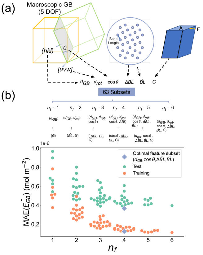
Figure 1: Feature Engineering. (a) Initial feature candidates based on the macroscopic geometry, microscopic bonding environment in the GB supercell, and the shear modulus of the elemental bulk system. (b) Best subset selection of features. There are a total of 63 possible subsets of 6 features. The swarmplot summarizes the performances of all the subsets, categorized by the number of features ($n_{f}$). The blue diamond point refers to the global optimal subset with the lowest test MAE in the predicted normalized grain boundary energy $\hat{E_{GB}}$.

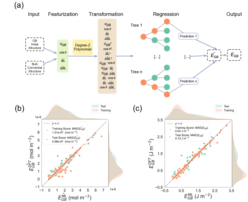
Figure 2: The machine learning pipeline and the performance. (a) The schematic illustration of the pipeline developed in this work. (b) and (c) are parity plots demonstrating the pipeline’s performances on $\hat{E_{GB}}$ and $E_{GB}$, respectively.

Figure 3 shows the permutation importance of the four input features, which is obtained by randomly shuffling the values of one feature and calculating the decrease in the MAE of the ML pipeline.[17] The feature with highest importance is $\bar{BL}$, the average bond length, while the remaining three GB features ($d_{GB}$, $\cos\theta$ and $\bar{\Delta BL}$) have similar feature importances. This is consistent with previous observations by Guziewski et al.[18] where the grain boundary energies of silicon carbide are better described by microscopic descriptors than the macroscopic ones. Furthermore, the fact that the $d_{GB}$ has higher importance than $\cos\theta$ echos with the conclusion drawn by Rohrer et al. [19], who found that variations in the grain boundary plane induce a greater change in the energy than the variations in the misorientation.

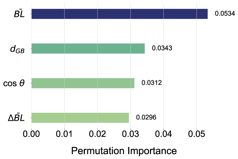
Figure 3: Permutation feature importance of the four geometric input features.

Thus far, the optimal model presented has been trained only on low $\Sigma$ GBs that can be readily computed using standard DFT computations. If it were limited to low $\Sigma$ GBs, such a model would be of limited utility. To demonstrate its ability to extrapolate to high $\Sigma$ GBs, which require far more expensive DFT computations, an additional 40 calculations on Ta, Pd, Cu, Pt and Li GBs with $\Sigma$ from 17 to 66 with MMI of the grain boundary plane $\leq$ 8 and MMI of the rotation axis $\leq$ 1 were performed (Figure LABEL:fig:data). The model, without further retraining, achieved an MAE($E_{GB}$) of 0.12 J m^-2  on this data set (Figure 4(b)), commensurate with the test error of the small $\Sigma$ GB test set.

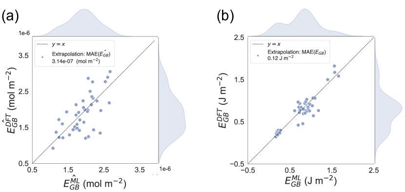
Figure 4: Performance of GB model on unseen high $\sigma$ GBs. Parity plot of predicted versus DFT (a) normalized $\hat{E_{GB}}$, (b) absolute $E_{GB}$.

To summarize, we have developed a physics-informed ML pipeline that predicts GB energies for more than 50 metals to within 0.13 J $m^{-2}$. This ML model can be applied to high $\Sigma$ GBs without loss in accuracy. A key innovation of our approach is to normalize the GB energy by the elemental cohesive energy to remove chemical scaling effects, resulting in a target that can be modelled purely using geometric and structural features. We believe this conceptual approach is general and is key to the development of ML models that are interpretable and extrapolatable. We have not attempted to model non-elemental GBs in this work given the lack of a sufficiently large dataset for model training. Nevertheless, we can speculate on the applicability of the same approach to GBs of non-elements, e.g., alloys and ceramics. Non-elemental GBs are much more complex, given that there may be compositional differences between the GB and the bulk region, e.g., preferential segregation of certain elements, etc [20]. While we believe some form of target normalization with an averaged bond energy descriptor, e.g., formation energies per atom, etc., would still be useful to remove large energetic scaling effects, it is likely be less effective than in the elemental case. Furthermore, a purely geometric / structural descriptor set would not be sufficient and compositional degrees of freedom would need to be included as well. Regardless of these limitations, we believe the conceptual framework developed in this work is sound and should be extended to other properties that have a well-defined scaling relationship with bond strength, e.g., elastic constants, etc.

All GB data and models have been made available in the Github repository of the open-source Materials Machine Learning (maml) package at https://github.com/materialsvirtuallab/maml.

References

- Tan et al. [2008] L. Tan, K. Sridharan, T. R. Allen, R. K. Nanstad, D. A. McClintock, Journal of Nuclear Materials 374 (2008) 270–280. doi:10.1016/j.jnucmat.2007.08.015.
- Shimada et al. [2002] M. Shimada, H. Kokawa, Z. J. Wang, Y. S. Sato, I. Karibe, Acta Materialia 50 (2002) 2331–2341. doi:10.1016/S1359-6454(02)00064-2.
- Zheng et al. [2020] H. Zheng, X.-G. Li, R. Tran, C. Chen, M. Horton, D. Winston, K. A. Persson, S. P. Ong, Acta Materialia 186 (2020) 40–49. doi:10.1016/j.actamat.2019.12.030.
- Kiyohara et al. [2016] S. Kiyohara, H. Oda, T. Miyata, T. Mizoguchi, Science Advances 2 (2016) e1600746. doi:10.1126/sciadv.1600746.
- Rosenbrock et al. [2017] C. W. Rosenbrock, E. R. Homer, G. Csányi, G. L. W. Hart, npj Computational Materials 3 (2017) 1–7. doi:10.1038/s41524-017-0027-x.
- Snow et al. [2019] B. D. Snow, D. D. Doty, O. K. Johnson, Front. Mater. 6 (2019). doi:10.3389/fmats.2019.00120.
- Gomberg et al. [2017] J. A. Gomberg, A. J. Medford, S. R. Kalidindi, Acta Materialia 133 (2017) 100–108. doi:10.1016/j.actamat.2017.05.009.
- Echeverri Restrepo et al. [2014] S. Echeverri Restrepo, S. Tamayo Giraldo, B. J. Thijsse, Computational Materials Science 86 (2014) 170–173. doi:10.1016/j.commatsci.2014.01.039.
- Friedman [2001] J. H. Friedman, The Annals of Statistics 29 (2001) 1189–1232. doi:10.1214/aos/1013203451.
- Ratanaphan et al. [2015] S. Ratanaphan, D. L. Olmsted, V. V. Bulatov, E. A. Holm, A. D. Rollett, G. S. Rohrer, Acta Materialia 88 (2015) 346–354. doi:10.1016/j.actamat.2015.01.069.
- Grimmer et al. [1974] H. Grimmer, W. Bollmann, D. H. Warrington, Acta Cryst A 30 (1974) 197–207. doi:10.1107/S056773947400043X.
- Wolf and Lutsko [1989] D. Wolf, J. F. Lutsko, Zeitschrift für Kristallographie - Crystalline Materials 189 (1989) 239–262. doi:10.1524/zkri.1989.189.14.239.
- Gibson and Schuh [2016] M. A. Gibson, C. A. Schuh, Scripta Materialia 113 (2016) 55–58. doi:10.1016/j.scriptamat.2015.09.041.
- Ong et al. [2013] S. P. Ong, W. D. Richards, A. Jain, G. Hautier, M. Kocher, S. Cholia, D. Gunter, V. L. Chevrier, K. A. Persson, G. Ceder, Computational Materials Science 68 (2013) 314–319. doi:10.1016/j.commatsci.2012.10.028.
- Read and Shockley [1950] W. T. Read, W. Shockley, Phys. Rev. 78 (1950) 275–289. doi:10.1103/PhysRev.78.275.
- Olson et al. [2016] R. S. Olson, N. Bartley, R. J. Urbanowicz, J. H. Moore, in: Proceedings of the Genetic and Evolutionary Computation Conference 2016, GECCO ’16, Association for Computing Machinery, New York, NY, USA, 2016, pp. 485–492. doi:10.1145/2908812.2908918.
- Breiman [2001] L. Breiman, Machine Learning 45 (2001) 5–32. doi:10.1023/A:1010933404324.
- Guziewski et al. [2021] M. Guziewski, D. Montes de Oca Zapiain, R. Dingreville, S. P. Coleman, ACS Appl. Mater. Interfaces 13 (2021) 3311–3324. doi:10.1021/acsami.0c15980.
- Rohrer [2011] G. S. Rohrer, J Mater Sci 46 (2011) 5881–5895. doi:10.1007/s10853-011-5677-3.
- Li et al. [2020] X.-G. Li, C. Chen, H. Zheng, Y. Zuo, S. P. Ong, npj Comput Mater 6 (2020) 1–10. doi:10.1038/s41524-020-0339-0.