Inertial Navigation Using an Inertial Sensor Array

Abstract

We present a comprehensive framework for fusing measurements from multiple and generally placed accelerometers and gyroscopes to perform inertial navigation. Using the angular acceleration provided by the accelerometer array, we show that the numerical integration of the orientation can be done with second-order accuracy, which is more accurate compared to the traditional first-order accuracy that can be achieved when only using the gyroscopes. Since orientation errors are the most significant error source in inertial navigation, improving the orientation estimation reduces the overall navigation error. The practical performance benefit depends on prior knowledge of the inertial sensor array, and therefore we present four different state-space models using different underlying assumptions regarding the orientation modeling. The models are evaluated using a Lie Group Extended Kalman filter through simulations and real-world experiments. We also show how individual accelerometer biases are unobservable and can be replaced by a six-dimensional bias term whose dimension is fixed and independent of the number of accelerometers.

I Introduction

Inertial navigation is the process of estimating the traveled distance and orientation of an object by time-integration of measured velocities and accelerations [1]. Due to the integrative nature of inertial navigation, the estimated position and orientation do inherently accumulate errors over time. This unbounded accumulation of position and orientation errors can only be limited by including external information from other sensor systems that provide an absolute reference to the environment or by including motion constraints. For instance, such aided inertial navigation has been done using satellite [2], video [3], radio [4], LIDAR [5], and magnetic field data [6]. Otherwise, the position and orientation errors’ growth rate can be reduced by decreasing the measurement errors of the inertial sensors or using additional motion information such as Zero-velocity Updates (ZUPTs) [7]. Improving the sensor hardware [8] reduces measurement errors, but this typically comes with increasing cost and sensor size. Another approach to reducing the measurement error is to fuse the measurements from a redundant amount of inertial sensors to produce a virtual sensor with higher accuracy. In particular, small Micro-Electro-Mechanical Systems (MEMS)-based inertial sensors can be cheaply fabricated [9] and are therefore suited for the construction of such sensor arrays [10, 11].

Fusing measurements from multiple accelerometers dispersed on a rigid body for inertial navigation has a long history [12, 13, 14, 15, 16]. When no gyroscopes are employed, this system is usually referred to as an Gyroscope-free Inertial Measurement Unit (GFIMU) or an accelerometer array. Since an accelerometer array provides information on the angular velocity and the angular acceleration, it can in principle replace gyroscopes for orientation estimation. Omission of gyroscopes for inertial navigation was in particular appealing for early MEMS-based sensors, since early MEMS-gyroscopes had inadequate performance and high energy consumption. However, the GFIMU cannot uniquely determine the instantaneous angular velocity and for low dynamic rotational motion, the estimation error of the angular velocity is high [17]. The angular acceleration also has to be time-integrated to unambiguously estimate the angular velocity [18], which imposes an extra time integration step compared to conventional inertial navigation. The extra integration step increases the error growth rate with an order of magnitude [19] and for certain configurations of the accelerometer array the resulting non-linear Ordinary Differential Equation (ODE) has been reported to be unstable [13, 20]. Mitigation of these problems can be achieved by placing the accelerometers in intricate configurations [19, 21, 22, 23, 14]. However, these configurations may impose infeasible geometric constraints on the system. Another approach has been to include a gyroscope to the GFIMU [24, 25, 26, 27, 28], a type of sensor assembly referred hereto as an inertial sensor array. To fuse the measurements from such an inertial sensor array, an ML estimator was presented in [17]. However, the estimator assumed calibrated sensors and used an iterative method to solve a non-linear optimization problem.

In this work, we present a comprehensive framework for fusing measurements from multiple and generally placed accelerometers and gyroscopes to perform inertial navigation. The traditional inertial navigation equations are extended to include the angular acceleration provided by the accelerometer array. The angular acceleration admits more accurate numerical integration of the orientation with second-order accuracy compared to the traditional first-order accuracy that can be achieved when only using the gyroscopes [1]. Since orientation errors are the most significant error source in inertial navigation, improving the orientation estimation will reduce the overall navigation error. To practically benefit from the angular acceleration, estimated by the accelerometer array, requires prior knowledge of the inertial sensor array. Therefore, we propose four state-space models, a.k.a mechanization equations, using different underlying assumptions regarding the time propagation of the orientation state. We evaluate these models using a Lie group Kalman filter through simulations and experiments. Using the Kalman filter, we show that the non linear problem of fusing the measurements of multiple accelerometers and gyroscopes can be solved by Kalman updates instead of using an iterative optimization method [17]. Moreover, the Kalman updates are also shown to stabilize the potentially unstable ODE when integrating the angular velocity. Finally, we note that individual accelerometer biases in an accelerometer array are unobservable [28]. However, we show that the individual accelerometer biases and the joint accelerometer covariance matrix can be replaced by a six-dimensional bias term and a six-by-six covariance matrix. The dimensions of these new terms are fixed and independent of the number of accelerometers.

II Inertial Navigation Modeling

This section presents the inertial navigation equations. First, we introduce the continuous-time equations for inertial sensor arrays to provide a rigorous derivation of the second-order integration of the orientation enabled by the array. Second, the continuous-time equations are discretized, and sensor models for accelerometers and gyroscopes are presented.

II-A Continuous-time Inertial Navigation Equations

The inertial navigation equations describe a moving body’s time evolution relative to a frame at rest [29]. This time-evolution or motion of the body is computed from measurements given by inertial sensors attached to the body. By convention, the moving frame and the frame at rest are denoted as the body frame and the navigation frame, respectively. Assuming that the body moves at such speeds that the Coriolis acceleration can be neglected, then the continuous-time equations for inertial navigation are given by [1]

$$\dot{R}^{nb} =R^{nb}[\omega^{b}\times],$$ (1a)

$$\dot{p}^{n} =v^{n},$$ (1b)

$$\dot{v}^{n} =g^{n}+R^{nb}s^{b}.$$ (1c)

Here $p^{n}$ is the body’s position in the navigation frame, $v^{n}$ is the velocity, $g^{n}$ is the local gravity, $\omega^{b}$ is the angular velocity between the navigation frame and the body frame, and $s^{b}$ is the specific force at the origin of the body frame. The superscripts $n$ and $b$ denote the navigation and body frame, respectively, and they indicate which coordinate frame a quantity is expressed in. The rotation matrix between these two frames is $R^{nb}$, which rotates a vector from the body frame to the navigation frame. Further, $[a\times]b=a\times b$ is the skew-symmetric matrix form of the cross-product. In conventional inertial navigation, the angular velocity $\omega^{b}$ and the specific force $s^{b}$ are measured by two sensor triads consisting of three orthogonal gyroscope and accelerometer sensors, respectively. Then (1) is time-integrated to yield estimates of $R^{nb}$, $p^{n}$, and $v^{n}$. The location of the accelerometer triad defines the origin of the body frame.

Assuming the body to be rigid and have multiple accelerometer triads geometrically dispersed on it, the specific force observed by individual accelerometer triads will differ when the rigid body undergoes a rotational motion [29]. The specific force at a point not located in the origin of the body frame, will have extra acceleration terms due to the centrifugal and Euler accelerations. These extra acceleration terms contain information about the rotation that can extend (1). Assuming that an accelerometer triad is located at $r_{k}^{b}$, the specific force at $r_{k}^{b}$ can then be related to the specific force at the origin of the body frame $s^{b}$ via [17]

$$f_{k}^{b}=s^{b}+\underbrace{[\omega^{b}\times]^{2}r_{k}^{b}}_{\begin{subarray}{c}\text{Centrifugal}\\ \text{acceleration}\end{subarray}}+\underbrace{[\dot{\omega}^{b}\times]r_{k}^{b}}_{\begin{subarray}{c}\text{Euler}\\ \text{acceleration}\end{subarray}}.$$ (2)

Here $\dot{\omega}^{b}$ is the angular acceleration of the rigid body. Since $[\dot{\omega}^{b}\times]r_{k}^{b}=-[r_{k}^{b}\times]\dot{\omega}^{b}$, it is noted that (2) is linear in $s^{b}$ and $\dot{\omega}^{b}$. Thus, by concatenating the measurements from $K$ accelerometer triads using (2) a differential equation for $\dot{\omega}^{b}$ and $s^{b}$ can be obtained as [12, 19, 14, 15, 16, 31]

$$\begin{bmatrix}\dot{\omega}^{b}\\ s^{b}\end{bmatrix}=\begin{bmatrix}A_{\dot{\omega}}\\ A_{s}\end{bmatrix}\left(f^{b}-h(\omega^{b},r_{1:K}^{b})\right),$$ (3)

where $r_{1:K}^{b}\triangleq\{r_{k}^{b}\}_{k=1}^{K}$,

$$f^{b} \triangleq\begin{bmatrix}f^{b}_{1}\\ \vdots\\ f^{b}_{K}\end{bmatrix}, h(\omega^{b},r_{1:K}^{b}) \triangleq\begin{bmatrix}[\omega^{b}\times]^{2}r_{1}^{b}\\ \vdots\\ [\omega^{b}\times]^{2}r_{K}^{b}\end{bmatrix}.$$ and (4)

The matrices $A_{\dot{\omega}}$ and $A_{s}$ are functions of the accelerometer positions $r_{k}^{b}$ and are further specified in Appendix A. The interpretation of (3) is that the difference in the specific force at $r_{k}^{b}$ and the centrifugal acceleration can be projected onto two different sub-spaces containing $\dot{\omega}^{b}$ and $s^{b}$, respectively. If it can be assumed that the accelerometer positions $r_{k}^{b}$ are centered in the body frame, i.e., $\sum_{k=1}^{K}r_{k}^{b}=0$, then $A_{\dot{\omega}}$ and $A_{s}$ become

$$A_{\dot{\omega}} \triangleq\begin{bmatrix}A_{1}&\cdots&A_{K}\end{bmatrix}, A_{s} \triangleq\frac{1}{K}\begin{bmatrix}I_{3}&\cdots&I_{3}\end{bmatrix},$$ (5a)

where

$$A_{k} \triangleq\left(\sum_{i=1}^{K}[r_{i}^{b}\times]^{\top}[r_{i}^{b}\times]\right)^{-1}[r_{k}^{b}\times],$$ (5b)

as shown in Appendix A. Here $I_{N}$ is the identity matrix of size $N$. For the inverse in (5b) to be well defined, and in general for the matrix $\begin{bmatrix}A_{\dot{\omega}}^{\top}&A_{s}^{\top}\end{bmatrix}^{\top}$ in (3) to have full rank, at least $K\geq 3$ accelerometer triads are required with positions that span a 2D plane [17]. With $A_{\dot{\omega}}$ and $A_{s}$ defined by (5) and $\sum_{k=1}^{K}r_{k}^{b}=0$, it is also shown in Appendix A that the differential equations in (3) decouple and become

$$\dot{\omega}^{b} =\sum_{k=1}^{K}A_{k}\left(f_{k}^{b}-[\omega^{b}\times]^{2}r_{k}^{b}\right),$$ (6a)

$$s^{b} =\frac{1}{K}\sum_{k=1}^{K}f_{k}^{b}.$$ (6b)

Hence, $s^{b}$ becomes independent of $\omega^{b}$. Equation (6b) could equivalently been derived by taking the mean of (2) and assuming $\sum_{k=1}^{K}r_{k}^{b}=0$.

It has been reported that for certain arrangements of the accelerometer positions and orientations the non linear ODE in (6a) and (3) are unstable[20, 12, 13]. Since a gyroscope triad measures the angular velocity, a feedback law using $\omega^{b}$ can be introduced to (6a) as

$$\dot{\omega}^{b}=\sum_{k=1}^{K}A_{k}\left(f_{k}^{b}-[\omega^{b}\times]^{2}r_{k}^{b}\right)-L\omega^{b},$$ (7)

for a matrix $L$. The matrix $L$ can be designed as $L=\operatorname{diag}(l_{x},l_{y},l_{z})$, and for sufficiently high $l_{i}$, the poles in (7) can be placed in the left-hand plane [32]. Thus, by providing feedback from a gyroscope triad the potentially unstable ODE in (6a) can be stabilized.

In summary, using an accelerometer array with multiple accelerometers triads dispersed on a rigid body, the inertial navigation equations in (1) can be extended with (6). Since the angular acceleration can, via (6a), be estimated only using the accelerometer triad measurements, it is strictly speaking not necessary to include a gyroscope triad for estimation of the rotation matrix in (1a). However, by including information from a gyroscope triad, the ODE is ensured to be stable.

II-B Discretized Inertial Navigation Equations

The continuous-time equations need to be discretized before implementation. When discretizing the traditional inertial navigation equations in (1) it is commonly assumed that the angular velocity and the specific force are constant between each sample instant [1]. However, since the inertial sensor array also provides an estimate of the angular acceleration, the discretization of the rotation matrix in (1a) can instead be based on the assumption of constant angular acceleration. For the angular velocity, position, and velocity, which are expressed in Euclidean vector-spaces, the discretization can be found by truncating the Taylor series given by

$$\omega(t+T) =\omega(t)+\dot{\omega}(t)T+\mathcal{O}(T^{2}),$$ (8a)

$$p(t+T) =p(t)+v(t)T+\dot{v}(t)\frac{T^{2}}{2}+\mathcal{O}(T^{3}),$$ (8b)

$$v(t+T) =v(t)+\dot{v}(t)T+\mathcal{O}(T^{2}).$$ (8c)

Here the superscripts related to the different frames have been omitted for notational brevity. Further, $t$ and $T$ denote the time and discretization (sample) period, respectively. Moreover, $\mathcal{O}(T^{n})$ denotes $n$:th and higher-order terms of $T$. However, integration by Taylor expansion is not possible for the rotation matrix $R$, since it belongs to $SO(3)=\{R\in\operatorname{\mathbb{R}}^{3\times 3}:R^{\top}R=I_{3},\det R=1\}$. That is, the orthogonality and determinant constraints impose $SO(3)$ to be a 3-dimensional manifold embedded in $\operatorname{\mathbb{R}}^{3\times 3}$. However, noting that $SO(3)$ is a matrix Lie group, Lie theory can be employed to integrate $R$ and discretize (1a). Instead of integrating in $\operatorname{\mathbb{R}}^{3\times 3}$, the integration is performed in the tangent space to $R$, also called the Lie algebra, which is isomorphic to $\operatorname{\mathbb{R}}^{3}$. For sufficiently small $T$ the solution to (1a) is [33]

$$R(t+T)=R(t)\exp_{SO(3)}^{\land}(\theta(T))$$ (9)

where $\exp_{SO(3)}^{\land}$ is the matrix exponential map from $\operatorname{\mathbb{R}}^{3}$ to $SO(3)$ [34]. Further, $\theta(T)$ is a vector found as the solution to

$$\dot{\theta}(\tau)=\Gamma(\theta(\tau))\omega(t+\tau),\quad\theta(0)=0,$$ (10)

where

$$\Gamma(\theta)=I_{3}+\frac{1}{2}[\theta\times]+\left(1-\frac{\|\theta\|}{2}\cot\left(\frac{\|\theta\|}{2}\right)\right)\frac{1}{\|\theta\|^{2}}[\theta\times]^{2}.$$ (11)

In the navigation literature, $\Gamma(\theta(t))$ is also known as the Bortz equation [35, 36, 37]. The physical interpretation of (9) is that $\theta$ can be considered an orientation deviation or perturbation of $R(t)$. The vector $\theta$ can also be interpreted as a rotation vector that rotates $R(t)$. For $\tau\in[0,T]$, the solution to (10) is given by the Taylor series

$$\theta(T)=\theta(0)+\dot{\theta}(0)T+\ddot{\theta}(0)\frac{T^{2}}{2}+\mathcal{O}(T^{3}).$$ (12)

Thus the approximate solution to the integration problem in (10) is given by calculating the time-derivatives of $\theta(\tau)$ and $\Gamma(\theta(\tau))$. In Appendix B, it is shown that (12) is equal to

$$\theta(T)=\omega(t)T+\dot{\omega}(t)\frac{T^{2}}{2}+\mathcal{O}(T^{3}).$$ (13)

This result was also used in [38] to integrate the rotation matrix while including the second-order term, i.e., $\dot{\omega}$. Note again that in conventional inertial navigation using an accelerometer and gyroscope triad the second-order term would not be used due to the absence of direct measurements of $\dot{\omega}$.

The discretized propagation equations for the navigation state are obtained by omitting the higher-order terms in the Taylor series. With a slight abuse of notation, we define the discrete samples as $R_{n}\triangleq R(t)$ and $R_{n+1}\triangleq R(t+T)$, and the other variables similarly. The discretized equations for the navigation state then become

$$R_{n+1} =R_{n}\exp_{SO(3)}^{\land}\left(\omega_{n}T+\dot{\omega}_{n}\frac{T^{2}}{2}\right),$$ (14a)

$$\omega_{n+1} =\omega_{n}+\dot{\omega}_{n}T,$$ (14b)

$$p_{n+1} =p_{n}+v_{n}T+(g+R_{n}s_{n})\frac{T^{2}}{2},$$ (14c)

$$v_{n+1} =v_{n}+(g+R_{n}s_{n})T.$$ (14d)

Here, the navigation equations for the inertial sensor array are propagated by the specific force $s_{n}$ and the angular acceleration $\dot{\omega}_{n}$. Assuming that the angular velocity is constant, that is $\dot{\omega}_{n}=0$, and removing (14b), then (14) reduces to the conventional discretized inertial navigation equations [1].

II-C Accelerometer Sensor Model

The accelerometer sensors are assumed to be calibrated in terms of scale factors, misalignment, and cross-coupling [39]. Further, the $k$:th accelerometer triad’s measurements at time-instant $n$ are assumed to be corrupted by white noise and a slowly time-varying bias [40]. That is, the accelerometer measurements $y_{k,n}^{(\text{a})}$ are modeled as

$$y_{k,n}^{(\text{a})} =f_{k,n}+b_{k,n}^{(\text{a})}+w_{k,n}^{(\text{a})},$$ (15a)

$$b_{k,n+1}^{(\text{a})} =b_{k,n}^{(\text{a})}+w^{(b,\text{a})}_{k,n},$$ (15b)

Here $b_{k,n}^{(\text{a})}$, $w_{k,n}^{(\text{a})}$ and $w^{(b,\text{a})}_{k}$ denote the accelerometer triad’s bias, measurement noise, and driving bias noise, respectively. The noise terms $w^{(\text{a})}_{k,n}$ and $w^{(b,\text{a})}_{k,n}$ are assumed to be zero mean, uncorrelated in time, uncorrelated with each others, and have covariances $Q^{(\text{a})}_{k}$ and $Q^{(b,\text{a})}_{k}$, respectively.

Since the accelerometer triads’ measurements only enter the navigation equations through weighted sums in the terms for the specific force $s_{n}$ and the angular acceleration $\dot{\omega}_{n}$ in (6), the individual accelerometer biases $b_{k,n}^{(\text{a})}$ will not be observable. To see this, inserting (15a) into (3) yields

$$\begin{bmatrix}\dot{\omega}_{n}\\ s_{n}\end{bmatrix}=\begin{bmatrix}A_{\dot{\omega}}\\ A_{s}\end{bmatrix}\left(y_{n}^{(\text{a})}-b_{n}^{(\text{a})}-w_{n}^{(\text{a})}-h(\omega_{n},r_{1:K})\right)$$ (16)

where

$$y_{n}^{(\text{a})} \triangleq\begin{bmatrix}y_{1,n}^{(\text{a})}\\ \vdots\\ y_{K,n}^{(\text{a})}\end{bmatrix}, b_{n}^{(\text{a})} \triangleq\begin{bmatrix}b_{1,n}^{(\text{a})}\\ \vdots\\ b_{K,n}^{(\text{a})}\end{bmatrix}, w_{n}^{(\text{a})} \triangleq\begin{bmatrix}w_{1,n}^{(\text{a})}\\ \vdots\\ w_{K,n}^{(\text{a})}\end{bmatrix}.$$ (17)

From (16), it is observed that $s_{n}$ and $\dot{\omega}_{n}$ depend on the vectors $b^{(\text{a})}$ and $w_{n}^{(\text{a})}$ only through the projection matrix $\begin{bmatrix}A_{\dot{\omega}}^{\top}&A_{s}^{\top}\end{bmatrix}^{\top}\in\operatorname{\mathbb{R}}^{6\times 3K}$ defined in (5). The projection matrix has full rank when $K\geq 3$ and when the accelerometer triads span a 2D plane [17]. If the full rank assumption is fulfilled, the vectors $b^{(\text{a})}\in\operatorname{\mathbb{R}}^{3K}$ and $w_{n}^{(\text{a})}\in\operatorname{\mathbb{R}}^{3K}$ are projected to the lower dimensional subspace $\operatorname{\mathbb{R}}^{6}$, meaning that there exists $3K-6$ dimensional subspaces of $b^{(\text{a})}$ and $w_{n}^{(\text{a})}$ that are unobservable. The dimension of the state-vector can thus be reduced to decrease the computational complexity and this also solves the problem of unobservable bias terms for individual accelerometers [28]. Similarly, the noise vector $w_{n}^{(a)}$ can be reduced. Define the new bias terms $b^{(\dot{\omega})}$ and $b^{(s)}$ and the new noise terms $w^{(\dot{\omega})}$ and $w^{(s)}$ as

$$\begin{bmatrix}b^{(\dot{\omega})}_{n}\\ b^{(s)}_{n}\end{bmatrix}\triangleq-\begin{bmatrix}A_{\dot{\omega}}\\ A_{s}\end{bmatrix}b^{(\text{a})}_{n},\quad\begin{bmatrix}w^{(\dot{\omega})}_{n}\\ w^{(s)}_{n}\end{bmatrix}\triangleq-\begin{bmatrix}A_{\dot{\omega}}\\ A_{s}\end{bmatrix}w^{(\text{a})}_{n}.$$ (18)

Then (16) can be rewritten as

$$\begin{bmatrix}\dot{\omega}_{n}\\ s_{n}\end{bmatrix}=\begin{bmatrix}A_{\dot{\omega}}\\ A_{s}\end{bmatrix}\left(y_{n}^{(\text{a})}-h(\omega_{n},r_{1:K})\right)+\begin{bmatrix}b_{n}^{(\dot{\omega})}\\ b_{n}^{(s)}\end{bmatrix}+\begin{bmatrix}w_{n}^{(\dot{\omega})}\\ w_{n}^{(s)}\end{bmatrix},$$ (19)

where the function $h$ is given in (3). The propagation equation for the new bias terms are

$$b^{(\dot{\omega})}_{n+1} =b^{(\dot{\omega})}_{n}+w^{(b,\dot{\omega})}_{n},$$ (20a)

$$b^{(s)}_{n+1} =b^{(s)}_{n}+w^{(b,s)}_{n},$$ (20b)

where the new driving bias noise terms $w^{(b,\dot{\omega})}_{n}$ and $w^{(b,s)}_{n}$ are introduced. The transformation in (18) will cause a correlation between $w^{(\dot{\omega})}_{n}$ and $w^{(s)}_{n}$. The joint covariance of for $w^{(\dot{\omega})}_{n}$ and $w^{(s)}_{w}$ is

$$\operatorname{\mathrm{Cov}}\left(\begin{bmatrix}w^{(\dot{\omega})}\\ w^{(s)}\end{bmatrix}\right)=\begin{bmatrix}A_{\dot{\omega}}Q^{(\text{a})}A_{\dot{\omega}}^{\top}&A_{\dot{\omega}}Q^{(\text{a})}A_{s}^{\top}\\ A_{s}Q^{(\text{a})}A_{\dot{\omega}}^{\top}&A_{s}Q^{(\text{a})}A_{s}^{\top}\end{bmatrix}.$$ (21)

The joint covariance for the new terms $w^{(b,\dot{\omega})}_{n}$ and $w^{(b,s)}_{w}$ can be derived analogously. From (19), we note first that the dimension of the new bias and noise terms are $6$ and independent of $K$. Second, it can be noted that the covariance matrix $Q^{(a)}$ that is used to propagate (3) is replaced with the covariance matrix in (21). The former has size $3K\times 3K$ and the latter has size $6\times 6$, meaning that the same noise structure can be represented with fewer elements.

Moreover, given the assumption of centered accelerometer positions, i.e., $\sum r_{k}=0$, and assuming that $Q^{(\text{a})}=\sigma_{a}^{2}I_{3K}$, then (21) simplifies to

$$\operatorname{\mathrm{Cov}}\left(\begin{bmatrix}w^{(\dot{\omega})}\\ w^{(s)}\end{bmatrix}\right)=\sigma_{a}^{2}\begin{bmatrix}\left(\sum_{k=1}^{K}[r_{k}\times]^{\top}[r_{k}\times]\right)^{-1}&0_{3,3}\\ 0_{3,3}&\frac{1}{K}I_{3}\end{bmatrix}.$$ (22)

In this case, the cross-correlation terms vanish. Further, it can be observed that the covariance of $w^{(s)}$ is inversely proportional to the number of accelerometer triads in the array and independent of the geometry. This is the same result as obtained in [17], and the covariance for the specific force is the same as the Cramér-Rao lower bound. Moreover, assuming that the accelerometer triads are mounted in a planar square grid with spacing $\alpha$, the covariance for $w^{(\dot{\omega})}$ is inversely proportional to $\alpha^{2}$, also a conclusion reached in [17].

II-D Gyroscope Sensor Model

The gyroscopes sensors are, similarly to the accelerometer sensors, assumed to be assembled in triads, and measure the angular velocity in three orthogonal directions. Moreover, the gyroscopes are also assumed to be calibrated in terms of scale factors, misalignment, and cross-coupling [39]. Since the angular velocity is identical for all points on a rigid body [29], the measurements from multiple geometrically dispersed gyroscope triads can be fused to create an equivalent virtual gyroscope triad [41]. Hence, for the purpose of this work, it can without loss of generality be assumed that there is only one gyroscope triad in the inertial sensor array. The measurements $y_{n}^{(\text{g})}$ from the equivalent virtual gyroscope triad can be modeled as

$$y_{n}^{(\text{g})} =\omega_{n}+b_{n}^{(\text{g})}+w_{n}^{(\text{g})},$$ (23a)

$$b_{n+1}^{(\text{g})} =b_{n}^{(\text{g})}+w^{(b,\text{g})}_{n}.$$ (23b)

Here $b^{(\text{g})}$, $w^{(\text{g})}$ and $w^{(b,\text{g})}$ are the gyroscope triad’s bias, measurement noise, and driving bias noise, respectively. The noise terms $w^{(\text{g})}_{n}$ and $w^{(b,\text{g})}$, are assumed to be zero mean, uncorrelated in time, and have covariances $Q^{(\text{g})}$ and $Q^{(b,\text{g})}$, respectively.

III Inertial Sensor Array Navigation Equations

This section presents the discretized inertial navigation equations and the sensor models combined into different state-space models. The models are constructed based on specific assumptions on the prior knowledge of the inertial sensor array. This section is concluded with a discussion on the advantages and disadvantages of the different models.

III-A State-Space Models

  2nd order accelerometer array state-space model   $\displaystyle R_{n+1}$ $\displaystyle=R_{n}\exp_{SO(3)}^{\land}\left(\omega_{n}T+\dot{\omega}_{n}\frac{T^{2}}{2}\right)\hskip 30.00005pt$ (24a) $\displaystyle\omega_{n+1}$ $\displaystyle=\omega_{n}+\dot{\omega}_{n}T$ (24b) $\displaystyle p_{n+1}$ $\displaystyle=p_{n}+v_{n}T+(g+R_{n}s_{n})\frac{T^{2}}{2}$ (24c) $\displaystyle v_{n+1}$ $\displaystyle=v_{n}+(g+R_{n}s_{n})T$ (24d) $\displaystyle b^{(\dot{\omega})}_{n+1}$ $\displaystyle=b^{(\dot{\omega})}_{n}+w^{(b,\dot{\omega})}_{n}$ (24e) $\displaystyle b^{(s)}_{n+1}$ $\displaystyle=b^{(s)}_{n}+w^{(b,s)}_{n}$ (24f) $\displaystyle b_{n+1}^{(\text{g})}$ $\displaystyle=b_{n}^{(\text{g})}+w^{(b,\text{g})}_{n}$ (24g) $\displaystyle\dot{\omega}_{n}$ $\displaystyle=b_{n}^{(\dot{\omega})}+w^{(\dot{\omega})}_{n}+\sum_{k}A_{k}(y_{k,n}^{(\text{a})}-[\omega_{n}\times]^{2}r_{k})$ (24h) $\displaystyle s_{n}$ $\displaystyle=b_{n}^{(s)}+w^{(s)}_{n}+\frac{1}{K}\sum_{k}y_{k,n}^{(\text{a})}$ (24i) $\displaystyle y_{n}^{(\text{g})}$ $\displaystyle=\omega_{n}+b^{(\text{g})}_{n}+w_{n}^{(\text{g})}$ (24j)   1st order accelerometer array state-space model   $\displaystyle R_{n+1}$ $\displaystyle=R_{n}\exp_{SO(3)}^{\land}\left(\omega_{n}T\right)\vphantom{\left(\omega_{n}T+\dot{\omega}_{n}\frac{T^{2}}{2}\right)}\hskip 80.00012pt$ (25a) $\displaystyle\omega_{n+1}$ $\displaystyle=\omega_{n}+\dot{\omega}_{n}T$ (25b) $\displaystyle p_{n+1}$ $\displaystyle=p_{n}+v_{n}T+(g+R_{n}s_{n})\frac{T^{2}}{2}$ (25c) $\displaystyle v_{n+1}$ $\displaystyle=v_{n}+(g+R_{n}s_{n})T$ (25d) $\displaystyle b^{(\dot{\omega})}_{n+1}$ $\displaystyle=b^{(\dot{\omega})}_{n}+w^{(b,\dot{\omega})}_{n}$ (25e) $\displaystyle b^{(s)}_{n+1}$ $\displaystyle=b^{(s)}_{n}+w^{(b,s)}_{n}$ (25f) $\displaystyle b_{n+1}^{(\text{g})}$ $\displaystyle=b_{n}^{(\text{g})}+w^{(b,\text{g})}_{n}$ (25g) $\displaystyle\dot{\omega}_{n}$ $\displaystyle=b_{n}^{(\dot{\omega})}+w^{(\dot{\omega})}_{n}+\sum_{k}A_{k}(y_{k,n}^{(\text{a})}-[\omega_{n}\times]^{2}r_{k})$ (25h) $\displaystyle s_{n}$ $\displaystyle=b_{n}^{(s)}+w^{(s)}_{n}+\frac{1}{K}\sum_{k}y_{k,n}^{(\text{a})}$ (25i) $\displaystyle y_{n}^{(\text{g})}$ $\displaystyle=\omega_{n}+b^{(\text{g})}_{n}+w_{n}^{(\text{g})}$ (25j)   2nd order gyroscope state-space model   $\displaystyle R_{n+1}$ $\displaystyle=R_{n}\exp_{SO(3)}^{\land}\left(\omega_{n}T+\dot{\omega}_{n}\frac{T^{2}}{2}\right)\hskip 30.00005pt$ (26a) $\displaystyle p_{n+1}$ $\displaystyle=p_{n}+v_{n}T+(g+R_{n}s_{n})\frac{T^{2}}{2}$ (26b) $\displaystyle v_{n+1}$ $\displaystyle=v_{n}+(g+R_{n}s_{n})T.$ (26c) $\displaystyle b^{(s)}_{n+1}$ $\displaystyle=b^{(s)}_{n}+w^{(b,s)}_{n}$ (26d) $\displaystyle b^{(\text{g})}_{n+1}$ $\displaystyle=b^{(\text{g})}_{n}+w^{(\text{g,b})}_{n}$ (26e) $\displaystyle s_{n}$ $\displaystyle=b_{n}^{(s)}+\frac{1}{K}\sum_{k}y_{k,n}^{(\text{a})}-w^{(\text{a})}_{k,n}$ (26f) $\displaystyle\omega_{n}$ $\displaystyle=y_{n}^{(\text{g})}-b^{(\text{g})}_{n}-w_{n}^{(\text{g})}$ (26g) $\displaystyle\dot{\omega}_{n}$ $\displaystyle=\sum_{k}A_{k}(y_{k,n}^{(\text{a})}-w^{(\text{a})}_{k,n}-[\omega_{n}\times]^{2}r_{k})$ (26h)   1st order gyroscope state-space model   $\displaystyle R_{n+1}$ $\displaystyle=R_{n}\exp_{SO(3)}^{\land}\left(\omega_{n}T\right)\vphantom{\dot{\omega}_{n}\frac{T^{2}}{2}}\hskip 80.00012pt$ (27a) $\displaystyle p_{n+1}$ $\displaystyle=p_{n}+v_{n}T+(g+R_{n}s_{n})\frac{T^{2}}{2}$ (27b) $\displaystyle v_{n+1}$ $\displaystyle=v_{n}+(g+R_{n}s_{n})T$ (27c) $\displaystyle b^{(s)}_{n+1}$ $\displaystyle=b^{(s)}_{n}+w^{(b,s)}_{n}$ (27d) $\displaystyle b^{(\text{g})}_{n+1}$ $\displaystyle=b^{(\text{g})}_{n}+w^{(\text{g,b})}_{n}$ (27e) $\displaystyle s_{n}$ $\displaystyle=b_{n}^{(s)}+\frac{1}{K}\sum_{k}y_{k,n}^{(\text{a})}-w^{(\text{a})}_{k,n}$ (27f) $\displaystyle\omega_{n}$ $\displaystyle=y_{n}^{(\text{g})}-b^{(\text{g})}_{n}-w_{n}^{(\text{g})}\vphantom{\sum_{k}A_{k}(y_{k,n}^{(\text{a})}-w^{(\text{a})}_{k,n}-[\omega_{n}\times]^{2}r_{k})}$ (27g)

Figure 1: Equations for the four proposed state-space models for inertial navigation using an inertial sensor array. The 2nd order models have a 2nd order term in the propagation of the rotation matrix in (24a) and (26a), while the 1st order models in (25a) and (27a) have a 1st order term. The accelerometer array models propagate the angular velocity in (24b) and (25b) using the angular acceleration computed from the accelerometer measurements in (24h) and (25h). The gyroscope models estimate the angular velocity directly using (26g) and (27g).

In the inertial sensor array, both the accelerometer array measurements and the gyroscope measurements can be used to estimate the angular velocity. The accelerometer array achieves this through time-integration of the angular acceleration, and the gyroscopes measure it directly. Since orientation estimation is an essential part of the inertial navigation process that amounts to time-integration of the angular velocity, we can either choose to use the accelerometer array, the gyroscope, or fuse both to estimate the orientation. Here, we present four different discrete state-space models shown in Fig. 1 of how to perform inertial navigation with an accelerometer array and a gyroscope triad, using different underlying assumptions regarding the time propagation of the orientation state.

In the first state-space model in (24), we incorporate all available information from both the accelerometer array and the gyroscope triad by collecting (14), (19), (20), and (23). In this model, the accelerometer array measurements are used to compute the angular acceleration, which propagates both the angular velocity and the rotation matrix using a 1st order and a 2nd order term, respectively. This is analogous to the specific force propagating the velocity and the position in (14d) and (14c). Thanks to the 2nd order term, the model is 2nd order accurate in the numerical integration of the rotation matrix. This model in (24) is from heron referred to as the 2nd order accelerometer array model.

If the accelerometer array is not sufficiently calibrated in terms of accelerometer positions, scale factors, misalignment, or cross-coupling, the estimation error of the angular acceleration might be prohibitively high. There are two ways of reducing the impact of a high estimation error in the angular acceleration in this case. First, the rotation matrix could be propagated only using a first-order term, which could be more accurate even though the numerical integration is now only 1st order accurate. This model is denoted the 1st order accelerometer array model and is shown in (25). The second option is to omit the propagation of the angular velocity while keeping the 2nd order term for the rotation matrix. This is possible since the angular acceleration in (6a) can be computed with the angular velocity given by the gyroscope measurements instead. The integration of the rotation matrix is thus 2nd order accurate, and this model is denoted as the 2nd order gyroscope model and is shown in (26). Here it is noted that the angular acceleration bias $b^{(\dot{\omega})}$ is not propagated, since that would include two bias terms for the propagation of $R_{n}$ in (26a), and would thus not be observable. But we could have also omitted the gyroscope bias $b^{(\text{g})}_{n}$ and kept $b^{(\dot{\omega})}_{n}$.

Moreover, the standard inertial navigation assumption could also be used, that is, the rotation matrix is propagated only using a 1st order term which is given by the gyroscopes. This model is denoted as the 1st order gyroscope model and is shown in (27). The only difference between this model and the standard inertial navigation equations is that the specific force is now calculated using the mean value of the accelerometer measurements.

III-B Discussion on State-Space Models

The main difference between the accelerometer array and gyroscope state-space models is whether the angular velocity is propagated or not in the navigation equations. In the accelerometer array models, the accelerometer array measurements are the sole input to the inertial navigation process and used both for calculating the translational and rotational changes. Hence, (24a) to (24i) and (25a) to (25i) can be used to realize a GFIMU inertial navigation system [14, 31, 20, 16]. The accelerometer array models could thus be used for high dynamic applications where gyroscopes usually saturate [42, 43]. If rotational information from gyroscopes are to be included this must be done via some filtering framework, such as the Kalman filter. In that case, (24a) to (24i) and (25a) to (25i), describe the system dynamics and (24j) and (25j) the observation equation of the state-space model used in the filtering process. A natural consequence of using the Kalman filter is that accelerometer and gyroscope measurements are fused using Kalman updates that have a fixed amount of computations. This is not the case for the current state-of-the-art method that fuses the accelerometer and gyroscope measurements by solving a non linear optimization problem using an iterative method [17]. The Kalman updates will also function as a feedback mechanism on $\omega$, which has the added benefit of stabilizing the potentially unstable continuous-time equation in (7) [20, 13]. Moreover, it is also possible to fuse the gyroscope and accelerometer array measurements for orientation estimation without Kalman updates as shown in the 2nd order gyroscope model. However, the gyroscope models will not work when the gyroscopes saturate.

IV Kalman Filter for Array Inertial Navigation

An inertial navigation solution is usually used in conjunction with other sensor systems. In this case, the sensor measurements are fused in a filtering framework, which is the topic of this section. Since the rotation matrix belongs to $SO(3)$, we present a Lie group Kalman filter for inertial navigation using the state-space models presented in Fig. 1. The filter equations for a general matrix Lie group are first presented, and then the specific equations for the 2nd order accelerometer array state-space model in (24) are presented. From this model, the other state-space models follow naturally.

IV-A Discrete Lie Group Extended Kalman Filter

Since the rotation matrix belongs to $SO(3)$ the standard Kalman filter cannot be directly used with the state-space models in Fig. 1. Here we instead employ the Discrete Lie-Group Extended Kalman Filter (D-LG-EKF) [44] that explicitly considers the non-Euclidean geometry of $SO(3)$. Since $\operatorname{\mathbb{R}}^{N}$ can be embedded into a matrix, the Euclidean space is also a matrix Lie group [34]. And since the composition of matrix Lie groups also is a matrix Lie group, we only present the D-LG-EKF for a single matrix Lie group $G$. The D-LG-EKF reduces to the standard Extended Kalman Filter (EKF) when $G$ is the Euclidean space [44].

The D-LG-EKF framework is based on the concept of concentrated Gaussian distributions on Lie groups [45]. The random variable $X$ defined on the Lie group $G$ has a Gaussian distribution with almost all of its probability mass concentrated in a small neighborhood around the mean $\hat{X}$, so that the probability distribution is effectively contained in the Lie algebra to $\hat{X}$. Since the Lie algebra is isomorphic to $\operatorname{\mathbb{R}}^{N_{x}}$, the Gaussian distribution can be represented by the Euclidean random variable $e\sim\mathcal{N}(0_{N_{x},1},P)$ where $P\in\operatorname{\mathbb{R}}^{N_{x}\times N_{x}}$ is a covariance matrix. Here $0_{N,M}$ is the zero matrix with $N$ rows and $M$ columns. The concentrated Gaussian distribution on $G$ is then defined as

$$X=\hat{X}\exp_{G}^{\land}\left(e\right).$$ (28)

Next, it is assumed in the D-LG-EKF framework that the state-space model is in the form

$$X_{n+1} =X_{n}\exp_{G}^{\land}\left(\Omega(X_{n},u_{n},w_{n}^{(\text{p})})\right),$$ (29a)

$$Y_{n} =\eta(X_{n})\exp_{G^{\prime}}^{\land}\left(w_{n}^{(\text{m})}\right),$$ (29b)

where $w_{n}^{(\text{p})}\in\operatorname{\mathbb{R}}^{N_{p}}$ is the process noise, $w_{n}^{(\text{m})}\in\operatorname{\mathbb{R}}^{N_{m}}$ is the measurement noise, and $u_{n}\in\operatorname{\mathbb{R}}^{N_{u}}$ is the input. The propagation function is $\Omega:G\times\operatorname{\mathbb{R}}^{N_{u}}\times\operatorname{\mathbb{R}}^{N_{p}}\rightarrow\operatorname{\mathbb{R}}^{N_{x}}$ and the measurement function is $\eta:G\rightarrow G^{\prime}$, as given by, e.g., (24). Next, it is assumed that the state estimate of $X_{n}$ to be a concentrated Gaussian with mean $\hat{X}_{n|n}$ and covariance $P_{n|n}$ according to (28), and that $w_{n}^{(\text{p})}\sim\mathcal{N}(0,Q^{(\text{p})})$ and $w_{n}^{(\text{m})}\sim\mathcal{N}(0,Q^{(\text{m})})$. Then, the propagation equations for the mean and the covariance are

$$\hat{X}_{n+1|n} =\hat{X}_{n|n}\exp_{G}^{\land}\left(\hat{\Omega}_{n}\right)$$ (30a)

$$P_{n+1|n} =F_{n}P_{n|n}F_{n}^{\top}+G_{n}Q^{(\text{p})}G_{n}^{\top}$$ (30b)

where

$$\hat{\Omega}_{n} =\Omega(\hat{X}_{n|n},u_{n},0),$$ (31a)

$$F_{n} =\operatorname{Ad}_{G}\left((\exp_{G}^{\land}\left(\shortminus\hat{\Omega}_{n}\right)\right)+\Phi_{n}(\hat{\Omega}_{n})J_{n}^{(x)},$$ (31b)

$$G_{n} =\Phi_{G}(\hat{\Omega}_{n})J_{n}^{(w)},$$ (31c)

$$J_{n}^{(x)} =\left.\frac{\partial}{\partial e}\Omega\left(\hat{X}_{n|n}\exp_{G}^{\land}\left(e\right),u_{n},0\right)\right\rvert_{e=0},$$ (31d)

$$J_{n}^{(w)} =\left.\frac{\partial}{\partial w}\Omega\left(\hat{X}_{n|n},u_{n},w\right)\right\rvert_{w=0}.$$ (31e)

Here $\operatorname{Ad}_{G}$ is the adjoint representation of $G$ on $\operatorname{\mathbb{R}}^{N_{x}}$ and $\Phi_{G}$ is the right Jacobian of $G$ [34]. The measurement update is

$$\hat{X}_{n|n} =\hat{X}_{n|n-1}\exp_{G}^{\land}\left(e_{n|n}\right)$$ (32a)

$$P_{n|n} =\Phi_{G}(e_{n|n})\left(I-K_{n}H_{n}\right)P_{n|n-1}\Phi_{G}(e_{n|n})^{\top}$$ (32b)

where

$$K_{n} =P_{n|n-1}H_{n}^{\top}\left(H_{n}P_{n|n-1}H_{n}^{\top}+Q^{(\text{m})}\right)^{-1}$$ (33a)

$$e_{n|n} =K_{n}\log_{G^{\prime}}^{\lor}\left(\eta(\hat{X}_{n|n-1})^{-1}Y_{n}\right)$$ (33b)

$$H_{n} =\shortminus\left.\frac{\partial}{\partial e}\log_{G^{\prime}}^{\lor}\left(\eta\left(\hat{X}_{n|n-1}\exp_{G}^{\land}\left(e\right)\right)^{-1}Y_{n}\right)\right\rvert_{e=0}.$$ (33c)

Here $\log_{G^{\prime}}^{\lor}$ is the matrix logarithm of $G^{\prime}$. If $G$ and $G^{\prime}$ were Euclidean spaces, (30) to (33) would be reduced to the regular EKF filter equations [44, 34]. Compared to the standard EKF filter equations, we can note the inclusion of the factors $\Phi_{G}(\hat{\Omega}_{n})$ and $\Phi_{G}(e_{n|n})$ for the computation of the covariance matrices. If $G=SO(3)$ these factors account for the rotation of the body frame and the correction of the covariance matrix for the rotation is also referred to as attitude reset [37].

IV-B D-LG-EKF for Array Inertial Navigation

Here we define the specific Lie-Group $G$ applicable for the inertial navigation equations. We derive the filter for the 2nd order accelerometer array state-space model in (24) and omit the other state-space models, since they can be derived from the 2nd order accelerometer array state-space model through deleting rows and columns in the Jacobians. For the state-space model in (24) the matrix Lie group is defined as ${G=SO(3)\times\operatorname{\mathbb{R}}^{18}}$. The explicit matrix expression for $G$ is found from the matrix embedding of the Euclidean elements by letting

$$z_{n}\triangleq\begin{bmatrix}\omega_{n}^{\top}&p_{n}^{\top}&v_{n}^{\top}&(b^{(\dot{\omega})}_{n})^{\top}&(b^{(s)}_{n})^{\top}&(b_{n}^{(\text{g})})^{\top}\end{bmatrix}^{\top}$$ (34)

and

$$X_{n} \triangleq\begin{bmatrix}R_{n}&0_{3,18}&0\\ 0_{18,3}&I_{18}&z_{n}\\ 0_{1,3}&0_{1,18}&1\end{bmatrix}=\begin{bmatrix}R_{n}\\ \omega_{n}\\ p_{n}\\ v_{n}\\ b^{(\dot{\omega})}_{n}\\ b^{(s)}_{n}\\ b_{n}^{(\text{g})}\end{bmatrix}_{G}.$$ (35)

The dimension of the Lie algebra of $G$ is consequently 21 and the state-covariance $P\in\operatorname{\mathbb{R}}^{21\times 21}$. Moreover, the process noise vector is composed of the accelerometer measurement noise and the white noise that drives the bias terms for the accelerometers and gyroscopes, that is,

$$w_{n}^{(\text{p})}\triangleq\begin{bmatrix}w_{n}^{(\dot{\omega})}\\ w_{n}^{(s)}\\ w_{n}^{(b,\dot{\omega})}\\ w_{n}^{(b,s)}\\ w_{n}^{(b,\text{g})}\end{bmatrix}.$$ (36)

The input to the propagation equation is the accelerometer measurements. The propagation equation is then derived from (24) as

$$\Omega(X_{n},y_{n}^{(\text{a})},w_{n}^{(\text{p})})=\begin{bmatrix}\omega_{n}T+\dot{\omega}_{n}\frac{T^{2}}{2}\\ \dot{\omega}_{n}T\\ v_{n}T+(g+R_{n}s_{n})\frac{T^{2}}{2}\\ (g+R_{n}s_{n})T\\ w_{n}^{(b,\dot{\omega})}\\ w_{n}^{(b,s)}\\ w_{n}^{(b,\text{g})}\end{bmatrix},$$ (37)

where $\dot{\omega}_{n}$ and $s_{n}$ are computed using (24h) and (24i). The Jacobians $F_{n}$ and $G_{n}$ are given in Appendix C.

Moreover, the angular velocity is propagated using the accelerometer measurements in (24b), but also provided by the gyroscopes in (24j). Hence, the gyroscope measurements have to be fused using Kalman updates in (32). The Lie-Group for gyroscope measurements is defined as $G^{(\text{g})}\triangleq\operatorname{\mathbb{R}}^{3}$ and the gyroscope measurement equation and its corresponding Jacobian is

$$\begin{bmatrix}I_{3}&y_{n}^{(\text{g})}\\ 0_{1,3}&1\\ \end{bmatrix} =\underbrace{\begin{bmatrix}I_{3}&\omega_{n}+b^{(\text{g})}_{n}\\ 0_{1,3}&1\\ \end{bmatrix}}_{\triangleq\eta^{(\text{g})}(X_{n})}\begin{bmatrix}I_{3}&w_{n}^{(\text{g})}\\ 0_{1,3}&1\\ \end{bmatrix}$$ (38a)

$$H^{(\text{g})} =\begin{bmatrix}0_{3}&I_{3}&0_{3,12}&I_{3}\end{bmatrix}.$$ (38b)

Here $0_{N}$ is the zero matrix of size $N$. As mentioned in Section III-B, the non linear optimization problem in [17] is now solved using Kalman updates in (32) and (38). The benefit of using Kalman updates is that the required number of computations are known in advance, which is not the case for iterative optimization methods.

Furthermore, a measurement update on the position can be made if the inertial navigation system has information on the position, e.g., when using a GPS sensor. The measurement equation and the corresponding Jacobian is given as

$$\begin{bmatrix}I_{3}&y_{n}^{(p)}\\ 0_{1,3}&1\\ \end{bmatrix} =\underbrace{\begin{bmatrix}I_{3}&p_{n}\\ 0_{1,3}&1\\ \end{bmatrix}}_{\triangleq\eta^{(p)}(X_{n})}\begin{bmatrix}I_{3}&w_{n}^{(p)}\\ 0_{1,3}&1\\ \end{bmatrix}$$ (39a)

$$H^{(p)} =\begin{bmatrix}0_{3,6}&I_{3}&0_{3,12}\end{bmatrix}.$$ (39b)

Here $y_{n}^{(p)}$ is the position measurement and $w_{n}^{(p)}$ is position measurement noise.

V Simulations and Experiments

Figure 2: Layout and dimensions of the inertial sensor array used in the experiments and simulations, along with the numbering of the IMU triads used in tables and figures. The dimensions denote the distance between the center positions of the IMU chip packages. The white dots on each IMU package are the orientation markers, indicating the mounting directions of the IMU packages [46]. The IMU packages on the underside, even numbers, are rotated $180$$\mathrm{\SIUnitSymbolDegree}$ around the axis $y=x$ relative to the IMU packages on the topside, odd numbers. Each IMU package measures $$4$~{}$\mathrm{m}\mathrm{m}$\times$4$~{}$\mathrm{m}\mathrm{m}$\times$1$~{}$\mathrm{m}\mathrm{m}$$ [46].

The performance of the proposed Kalman filter and the four proposed state-space models for inertial navigation using an inertial sensor array was evaluated by simulations and experiments. The simulations demonstrate the performance obtained under idealized assumptions, and real-world experiments verify the practical applicability of the proposed methods.

V-A Simulations

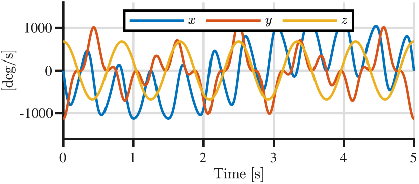
(a) High dynamics

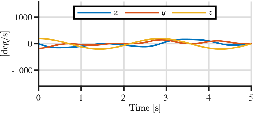
(b) Low dynamics

Figure 3: The angular velocity for the motion used in the simulations, where LABEL:sub@fig:sim_w_motion_high and LABEL:sub@fig:sim_w_motion_low represent high and low rotational dynamics, respectively.

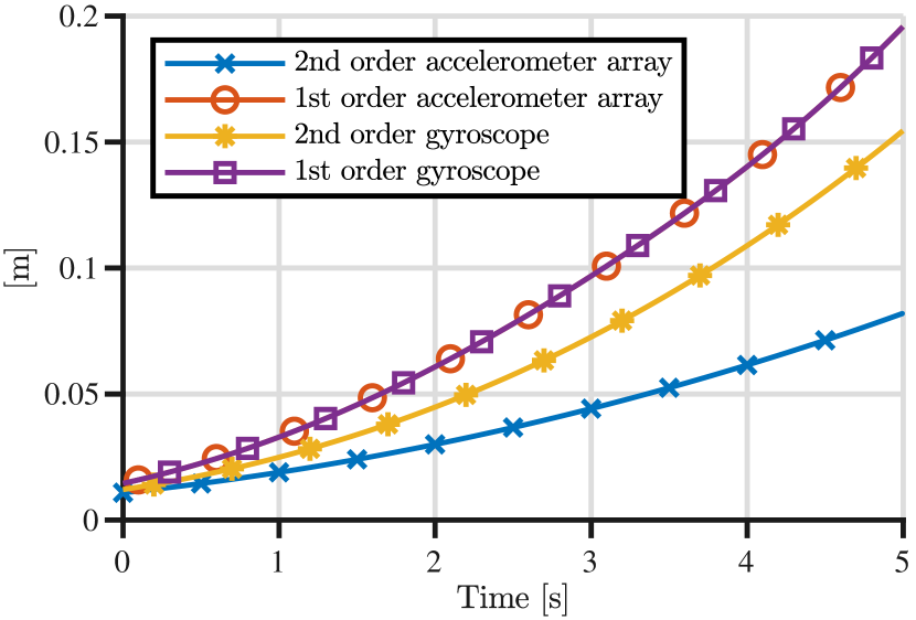
(a) Low dynamics, $F_{s}=500$ Hz

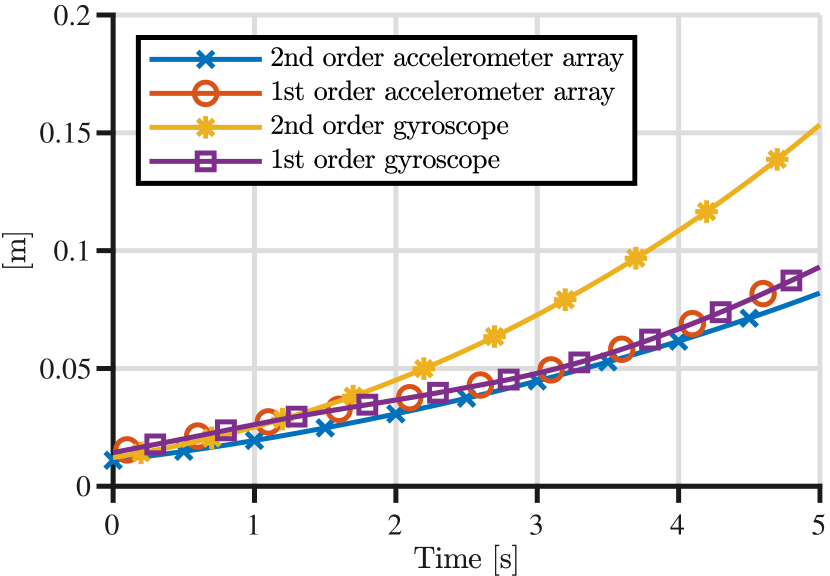
(b) High dynamics, $F_{s}=500$ Hz

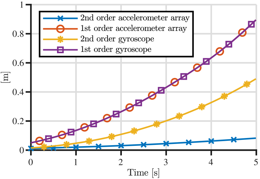
(c) Low dynamics, $F_{s}=100$ Hz

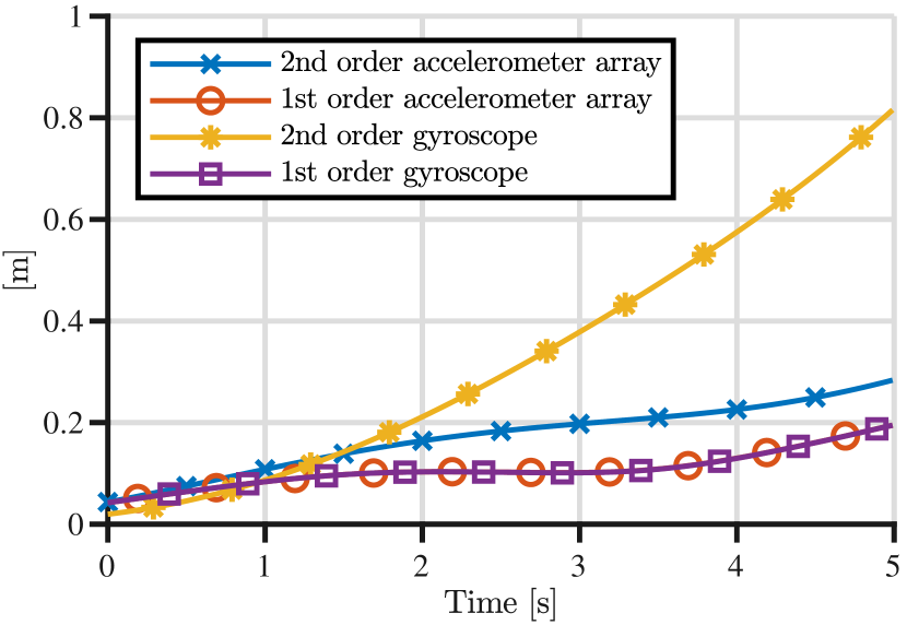
(d) High dynamics, $F_{s}=100$ Hz

Figure 4: The position estimation RMSE of the four proposed state-spaces models in (24) to (27) using simulated data. LABEL:sub@fig:simulations_pos_rmse_low_dynamics_high_Fs, LABEL:sub@fig:simulations_pos_rmse_high_dynamics_high_Fs, LABEL:sub@fig:simulations_pos_rmse_low_dynamics_low_Fs, and LABEL:sub@fig:simulations_pos_rmse_high_dynamics_low_Fs show the RMSE for different rotational dynamics as shown in Fig. 3 and for different sampling frequencies $F_{s}$.

We evaluated the performance of the proposed inertial navigation system realizations in Fig. 1 using simulated data corresponding to different sampling frequencies $F_{s}$, and to different degrees of rotational dynamics. The inertial sensor array considered in the simulations is shown in Fig. 2, which is an inertial sensor array with 32 IMUs attached to a Printed Circuit Board (PCB). The accelerometers and gyroscopes are assumed to be perfectly calibrated in terms of scale factors, misalignment, cross-coupling, and accelerometer positions [39, 47, 48]. Hence, the sensor measurements are assumed only to be corrupted by a constant bias and white noise. Specifically, we assume the noise of the accelerometers and the gyroscopes to be zero-mean, uncorrelated and to have a standard deviation of $\sigma^{(\text{a})}=$0.5$~{}$\mathrm{m}\mathrm{/}\mathrm{s}^{2}$$ and $\sigma^{(\text{g})}=$1$~{}$\deg\mathrm{/}\mathrm{s}$$, respectively. The constant bias is assumed to be drawn from a normal distribution with standard deviation set to $\sigma^{(\text{a})}$ and $\sigma^{(\text{g})}$ for the accelerometers and gyroscope, respectively. These parameters were selected to reflect the performance of typical MEMS-based IMUs [46]. Further, we assume idealistically that the sensors have an infinite dynamic range.

Field conditions were simulated by generating a continuous sinusoidal motion from which artificial sensor measurements were constructed. To account for the unknown constant bias, artificial position measurements were simulated for an initial time period to let the bias estimate of the filters converge. After convergence, the position updates ceased and the filters conducted pure inertial navigation. More specifically, the angular velocity in the simulations was set to two different sinusoids as shown in Fig. 3, depicting low dynamic rotational and a high dynamic rotational motion. From the generated continuous-time motion sequence discrete time sensor measurements were generated considering two different sampling frequencies, $F_{s}=500~{}$\mathrm{H}\mathrm{z}$$ and $F_{s}=100~{}$\mathrm{H}\mathrm{z}$$, designating high and low sampling frequencies, respectively. The synthetic navigation position measurements were generated from the true motion and with an added zero-mean noise with a standard deviation of $\sigma^{(p)}=$10$~{}$\mathrm{c}\mathrm{m}$$ and with a frequency of $100~{}$\mathrm{H}\mathrm{z}$$. The filters had $\sigma^{(b,\text{g})}$, $\sigma^{(b,s)}$ and $\sigma^{(b,\dot{\omega})}$ all equal to zero. The initial values for the accelerometer and gyroscope biases were set to zero and the corresponding initial covariances were set to $\sigma^{(b,\text{g})}_{0}=3\sigma^{(\text{g})}$, $\sigma^{(\text{a})}_{0}=3\sigma^{(\text{a})}$, with $\sigma^{(b,s)}_{0}$ and $\sigma^{(b,\dot{\omega})}_{0}$ evaluated using (22).

The Root-Mean-Square Error (RMSE) of the navigation position of the filters during the inertial navigation phase is shown in Fig. 4 for 1000 Monte Carlo simulations. We first observe that the 1st order state-space models in (25) and (27) give similar results for all considered cases meaning that fusing the accelerometer array’s and the gyroscopes’ measurements for angular velocity estimation yields little improvement over integrating the angular velocity directly from the gyroscope measurements. Moreover, for the low dynamic rotational motion, we observe a reduced error of the 2nd order models in (24) and (26) meaning that the 2nd order numerical integration of the rotation matrix using the angular acceleration reduces the overall position error growth. However, this is not the case for highly dynamic rotational motion, where the reduced error diminishes and even exceeds that of the 1st order models in (25) and (27) for low sampling frequencies. This could be attributed to the fact that the angular acceleration estimate has its lowest variance when the angular velocity is zero [17], and thus the 2nd order integration scheme for the rotation matrix becomes more accurate for low dynamic rotational motions. With increasing rotational motion, the variance in angular acceleration increases and the 2nd order term in the rotation matrix becomes increasingly less accurate. The same conclusions seem to hold for both high and low sampling frequencies, indicating that the numerical integration of the angular velocity is not unstable. Evaluating the poles of the Jacobian to (6a) using the nominal values of the accelerometer positions of the inertial sensor array yields three eigenvalues on the imaginary axis, meaning that the time-continuous equations are stable.

V-B Experiments

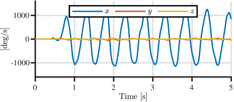
(a) High dynamics

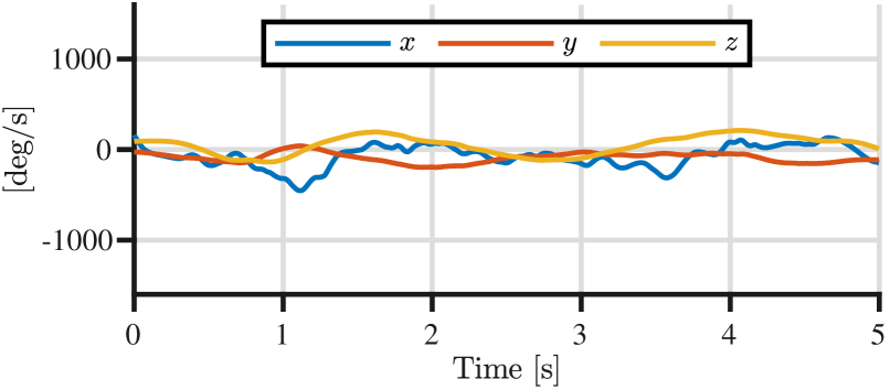
(b) Low dynamics

Figure 5: The angular velocity computed by the mean of 32 gyroscope triads from experiment 1, where LABEL:sub@fig:exp_w_motion_high and LABEL:sub@fig:exp_w_motion_low represent high and low rotational dynamics, respectively.

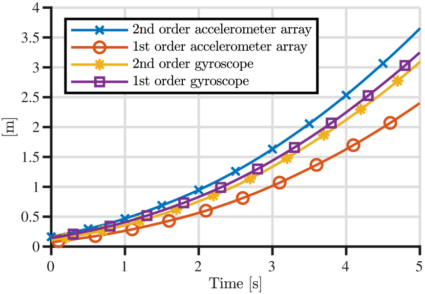
(a) Low dynamics, $F_{s}=500$ Hz

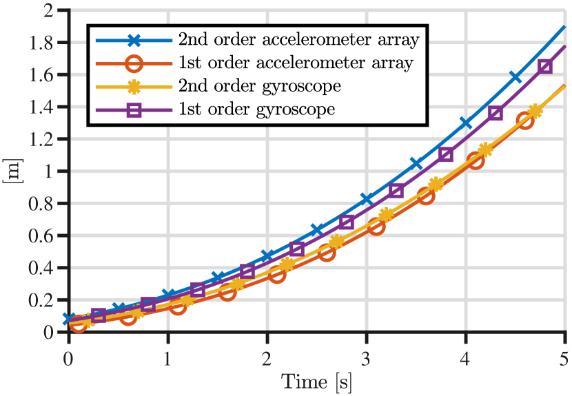
(b) High dynamics, $F_{s}=500$ Hz

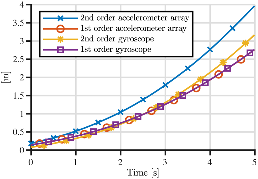
(c) Low dynamics, $F_{s}=100$ Hz

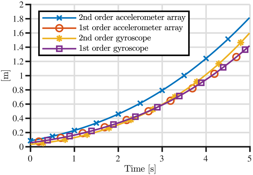
(d) High dynamics, $F_{s}=100$ Hz

Figure 6: The position estimation RMSE of the four proposed state-spaces models in (24) to (27) using experimental data. LABEL:sub@fig:experiments_pos_rmse_low_dynamics_high_Fs, LABEL:sub@fig:experiments_pos_rmse_high_dynamics_high_Fs, LABEL:sub@fig:experiments_pos_rmse_low_dynamics_low_Fs, and LABEL:sub@fig:experiments_pos_rmse_high_dynamics_low_Fs show the RMSE for different rotational dynamics as shown in Fig. 5 and for different sampling frequencies $F_{s}$.

We also evaluated the performance of proposed inertial navigation system realizations in Fig. 1 using real experiments performed on the array in Fig. 2. We collected measurements from the array while simultaneously measuring the position of the array using a camera-based Motion Capture (MC) system. We assume that the inertial sensor array samples all the IMUs simultaneously and instantaneously during one time sample. The details about the hardware and the sampling process can be found in [49]. The inertial sensor array was attached to a rig that had multiple reflective markers that were tracked by the cameras. The MC system provided both a rotation and position estimate of the rig with a sampling frequency of $100~{}$\mathrm{H}\mathrm{z}$$.

The rig was then exposed to twisting motion in seven different experiments. Each experiment consisted of three phases, a time-synchronization phase, a low rotational dynamics phase, and a high rotational dynamics phase. The time-synchronization phase consisted of the rig and the inertial sensor array being rotated around a single axis. This rotating motion generated a high Signal-to-Noise Ratio (SNR) signal from the gyroscopes, which was compared with the computed angular velocity from the rotation estimates given by the MC system. An illustration of the rotational motion during the low and high dynamic phases is shown in Fig. 5, where the angular velocity of the gyroscopes in experiment 1 is shown. Due to difficulties in aligning the origin of the MC frame and the origin of the inertial sensor array, the standard deviation for the position updates was set to $\sigma^{(p)}=$10$~{}$\mathrm{c}\mathrm{m}$$.

In each experiment, the four filters were used to process the measurement from the inertial sensor array with the same noise variances settings as used in the simulations in Section V-A. Position measurements given by the MC system were also fed to the filters up to a certain time point, and then the position updates ceased. The filters then performed pure inertial navigation for 5 seconds. The accelerometer and gyroscope biases were initialized to zero, and the filters ran for a long enough time period for the bias estimates to converge before the pure inertial navigation phase was started. Inertial navigation commenced from 20 equally spaced time-instants during the low dynamic and high dynamic phases. For each rotational phase the RMSE during the inertial navigation phase was computed by averaging the position over the 140 times the position updates ceased and over the coordinate axes.

The RMSE of the position estimates for the experiments is shown in Fig. 6 for two different sampling frequencies. First, we note that the 2nd order accelerometer array model in (24) has a higher RMSE compared to all other models for all considered cases. And the expected improvement of the 2nd order models in (24) and (26) is not seen as observed in the simulations. Thus, joint propagation of the angular velocity and the rotation matrix using the angular acceleration has a higher error than solely propagating the rotation matrix only using the gyroscope measurements. This suggests that there is an estimation error in the angular acceleration computed with the accelerometer array measurements, which could depend on several factors such as misspecified covariances, scale factor errors, sensitivity axes misalignments, cross-coupling terms, and uncertainties in the accelerometer positions. However, for the high-frequency sampling case, the 2nd order gyroscope model in (26) and the 1st order accelerometer array in (25) have a lower error compared to the 1st order gyroscope model in (27), meaning that the estimated angular acceleration can improve the orientation estimation. And for the 100 Hz sampling frequency, we observe that the RMSE for the accelerometer array models in (24) and (25) increase relative to the 1st order gyroscope model in (27). Thus, when the integration time increases the error in the orientation estimation using the angular acceleration increases, suggesting that the angular velocity integration is not stable. Since the simulations did not suggest an unstable integration for the considered geometry of the accelerometer positions, it is left for future research to find the cause for the observed behavior.

VI Summary and Conclusions

We propose four state-space models of how to perform inertial navigation using an inertial sensor array. Using different underlying assumptions regarding the orientation modeling, these four models fuse the measurements of multiple and generally placed accelerometer triads and a gyroscope triad to improve inertial navigation performance. The non linear problem of fusing the accelerometer array measurements and the gyroscope measurements for angular velocity estimation is solved through Kalman updates. The benefit of using Kalman updates is twofold. First, the required computations for the sensor fusion problem can be known in advance, which is not the case when this fusion is done using an iterative optimization method [17]. Knowing the number of computations in advance is useful for embedded systems where computational resources are limited. Second, we show that the Kalman updates stabilize the potentially unstable equations when the angular velocity is integrated using the accelerometer array measurements [20, 13]. Thus, it is not necessary to place the accelerometer triads in complex geometries to ensure stability [19, 21, 22, 23, 14]. Furthermore, the angular acceleration is estimated from the accelerometer array measurements and we present three methods for how to capitalize on the angular acceleration: • either 1) propagate the angular velocity; or 2) propagate the rotation matrix with 2nd order accuracy; or 3) both. We also show that the correct weighting of multiple accelerometer measurements for computation of the specific force is given by the mean value [50], which is derived using the implicit assumption of centered accelerometer positions. Moreover, we show how only six dimensions of all individual accelerometer biases are observable and consequently, it is sufficient to only model the bias in six dimensions independent of the number of accelerometer triads. This observation answers the question posed in [28] where it was observed that the individual biases of the accelerometers were unobservable, and that only three dimensions of all bias terms were observable when computing the specific force.

Moreover, simulations showed that for low rotational motions a significant reduction in navigation position error can be achieved compared to the conventional inertial navigation method when using all available information from the accelerometer array and the gyroscopes. This can be attributed to the increased accuracy in the numerical integration of the rotation matrix by the inclusion of a 2nd order term given by the angular acceleration. However, this error reduction was not observed in real-world experiments. This can be ascribed to errors in the assumed covariances, accelerometer positions, scale-factors, and misalignments. Thus, future research should focus on methods to calibrate and compensate for these error sources. However, it was observed from the experiments that the inertial sensor array could, for high sampling frequencies, provide extra orientation information and reduce the inertial navigation error compared to conventional inertial navigation.

Appendix A Accelerometer Array Differential Equations

Concatenating the measurements from $K$ accelerometer triads using (2) yields

$$f^{b}=h(\omega^{b},r_{1:K}^{b})+H(r_{1:K}^{b})\begin{bmatrix}\dot{\omega}^{b}\\ s^{b}\end{bmatrix}$$ (40)

where $f^{b}$ and $h$ are defined in (4) and

$$H(r_{1:K}^{b})\triangleq\begin{bmatrix}-[r_{1}^{b}\times]&I_{3}\\ \vdots&\vdots\\ -[r_{K}^{b}\times]&I_{3}\end{bmatrix}.$$ (41)

The solution for the angular accelerations and the specific force is then

$$\begin{bmatrix}\dot{\omega}^{b}\\ s^{b}\end{bmatrix}=A\left(f^{b}-h(\omega^{b},r_{1:K}^{b})\right),$$ (42)

where

$$A\triangleq\left(H^{\top}H\right)^{-1}H^{\top}.$$ (43)

The angular acceleration and the specific force are thus different linear combinations determined by the matrix $A$ of the difference between the specific forces $f_{k}$ and the centrifugal accelerations $h(\omega^{b},r_{1:K}^{b})$. Equation (42) can be simplified by noting that

$$H^{\top}H=\begin{bmatrix}\sum_{k}[r_{k}^{b}\times]^{\top}[r_{k}^{b}\times]&-\sum_{k}[r_{k}^{b}\times]^{\top}\\ -\sum_{k}[r_{k}^{b}\times]&KI_{3}\end{bmatrix}.$$ (44)

Assuming that $\sum_{k}r_{k}^{b}=0$, and consequently $\sum_{k}[r_{k}^{b}\times]=0$, yields

$$H^{\top}H=\begin{bmatrix}\sum_{k}[r_{k}^{b}\times]^{\top}[r_{k}^{b}\times]&0\\ 0&KI_{3}\end{bmatrix}.$$ (45)

The three last rows of (42) then become

$$\frac{1}{K}\sum_{k=1}^{K}(f_{k}^{b}-[\omega^{b}\times]^{2}r_{k}^{b})=\frac{1}{K}\sum_{k=1}^{K}f_{k}^{b},$$ (46)

which are independent of $\omega^{b}$. The differential equations in (42) then decouples and become (6).

Appendix B Time Evolution of Rotation Vector

To show that (12) is equal to (13) amounts to calculating the terms $\dot{\theta}(0)$ and $\ddot{\theta}(0)$. The rotation vector can be expressed as $\theta=\|\theta\|u$ where $\|\theta\|$ is the magnitude of $\theta$ and $u$ is the unit vector pointing in the same direction as $\theta$. Using this, (11) can be rewritten as

$$\Gamma(\theta)=I_{3}+\frac{1}{2}\|\theta\|[u\times]+\left(1-\frac{\|\theta\|}{2}\cot\left(\frac{\|\theta\|}{2}\right)\right)[u\times]^{2}.$$ (47)

It is then clear that $\Gamma(0)=I_{3}$. With $\theta(0)=0$ the first time-derivative of $\theta$ is

$$\dot{\theta}(0)=\Gamma(\theta(0))\omega(t)=\omega(t).$$ (48)

Next $\ddot{\theta}(0)$ is obtained through

$$\ddot{\theta}(\tau)=\dot{\Gamma}(\theta(\tau))\omega(t+\tau)+\Gamma(\theta(\tau))\dot{\omega}(t+\tau).$$ (49)

By differentiation, it can be shown that

$$\left.\dot{\Gamma}(\theta(\tau))\right|_{\tau=0}=-\frac{1}{2}[\omega(t)\times],$$ (50)

so that

$$\ddot{\theta}(0)=-\frac{1}{2}[\omega(t)\times]\omega(t)+\dot{\omega}(t)=\dot{\omega}(t).$$ (51)

Appendix C Jacobians

The Jacobian in (31d) to (37) in the state-matrix $X_{n}$ is given by

$$J_{n}^{(x)}=\begin{bmatrix}J_{n}^{(1)}&J_{n}^{(2)}\\ 0_{9,12}&0_{9}\end{bmatrix},$$ (52)

where

$$J_{n}^{(1)} =\begin{bmatrix}0_{3}&I_{3}T+\frac{\partial\dot{\omega}_{n}}{\partial\omega}\frac{T^{2}}{2}&0_{3}&0_{3}\\ 0_{3}&\frac{\partial\dot{\omega}_{n}}{\partial\omega}T&0_{3}&0_{3}\\ \frac{\partial\dot{v}_{n}}{\partial e_{R}}\frac{T^{2}}{2}&0_{3}&0_{3}&I_{3}T\\ \frac{\partial\dot{v}_{n}}{\partial e_{R}}T&0_{3}&0_{3}&0_{3}\end{bmatrix},$$ (53a)

and

$$J_{n}^{(2)} =\begin{bmatrix}\frac{\partial\dot{\omega}_{n}}{\partial b^{(\dot{\omega})}}\frac{T^{2}}{2}&0_{3}&0_{3}\\ \frac{\partial\dot{\omega}_{n}}{\partial b^{(\dot{\omega})}}T&0_{3}&0_{3}\\ 0_{3}&\frac{\partial\dot{v}_{n}}{\partial b^{(s)}}\frac{T^{2}}{2}&0_{3}\\ 0_{3}&\frac{\partial\dot{v}_{n}}{\partial b^{(s)}}T&0_{3}\end{bmatrix}.$$ (53b)

Here $e_{R}\in\operatorname{\mathbb{R}}^{3}$ is the Lie algebra variable to $R$. The partial derivatives of $\dot{\omega}_{n}$ are given by

$$\frac{\partial\dot{\omega}_{n}}{\partial\omega} =\sum_{k}A_{k}\left([[\omega_{n}\times]r_{k}\times]+[\omega_{n}\times][r_{k}\times]\right),$$ (54a)

$$\frac{\partial\dot{\omega}_{n}}{\partial b^{(\dot{\omega})}} =I_{3},$$ (54b)

derivatives of $\dot{v}_{n}$ are given by

$$\frac{\partial\dot{v}_{n}}{\partial e_{R}} =-R_{n}\left[s_{n}\times\right], \frac{\partial\dot{v}_{n}}{\partial b^{(s)}} =I_{3}.$$ (55)

The Jacobian in (31e) to (37) in the noise vector $w_{n}^{(p)}$ is given by

$$J_{n}^{(w)} =\begin{bmatrix}\frac{\partial\dot{\omega}_{n}}{\partial w_{n}^{(\dot{\omega})}}\frac{T^{2}}{2}&0_{3,9}\\ \frac{\partial\dot{\omega}_{n}}{\partial w_{n}^{(\dot{\omega})}}T&0_{3,9}\\ \frac{\partial\dot{v}_{n}}{\partial w_{n}^{(s)}}\frac{T^{2}}{2}&0_{3,9}\\ \frac{\partial\dot{v}_{n}}{\partial w_{n}^{(s)}}T&0_{3,9}\\ 0_{9,3}&I_{9}\end{bmatrix}$$ (56a)

where the partial derivatives are given by

$$\frac{\partial\dot{\omega}_{n}}{\partial w_{n}^{(\dot{\omega})}} =I_{3}, \frac{\partial\dot{v}_{n}}{\partial w_{n}^{(\text{a})}} =I_{3}.$$ (57)

References

- [1] D. Titterton and J. Weston, Strapdown Inertial Navigation Technology. London, UK: The Institution of Engineering and Technology, 2004.
- [2] J. A. Farrell, Aided Navigation Systems: GPS and High Rate Sensors. New York, NY, USA: McGraw-Hill, Inc., 2008.
- [3] G. Huang, “Visual-Inertial Navigation: A Concise Review,” in Int. Conf. Robotics Automation (ICRA), Montreal, QC, Canada, May 2019, pp. 9572–9582.
- [4] A. D. Angelis, J.-O. Nilsson, I. Skog, P. Händel, and P. Carbone, “Indoor Positioning by Ultrawide Band Radio Aided Inertial Navigation,” in XIX IMEKO World Congr. Fundamental Applied Metrology, Lisbon, Portugal, Sep. 2009, pp. 574–579.
- [5] J. Tang, Y. Chen, X. Niu, L. Wang, L. Chen, J. Liu, C. Shi, and J. Hyyppä, “LiDAR scan matching aided inertial navigation system in GNSS-denied environments,” Sensors, vol. 15, no. 7, pp. 16 710–16 728, July 2015.
- [6] M. Kok, N. Wahlström, T. B. Schön, and F. Gustafsson, “MEMS-based inertial navigation based on a magnetic field map,” in IEEE Int. Conf. Acoustics, Speech Signal Processing (ICASSP), Vancouver, BC, Canada, May 2013, pp. 6466–6470.
- [7] J. Wahlström and I. Skog, “Fifteen Years of Progress at Zero Velocity: A Review,” IEEE Sensors J., vol. 21, no. 2, pp. 1139–1151, Jan. 2021.
- [8] A. D. King, “Inertial navigation-forty years of evolution,” GEC review, vol. 13, no. 3, pp. 140–149, 1998.
- [9] D. K. Shaeffer, “MEMS inertial sensors: A tutorial overview,” IEEE Commun. Mag., vol. 51, no. 4, pp. 100–109, Apr. 2013.
- [10] J.-O. Nilsson and I. Skog, “Inertial sensor arrays - A literature review,” in European Navigation Conf. (ENC), Helsinki, Finland, May 2016, pp. 1–10.
- [11] M. W. Givens and C. Coopmans, “A Survey of Inertial Sensor Fusion: Applications in sUAS Navigation and Data Collection,” in Int. Conf. Unmanned Aircraft Systems (ICUAS), Atlanta, GA, USA, June 2019, pp. 1054–1060.
- [12] A. R. Schuler, A. Grammatikos, and K. A. Fegley, “Measuring Rotational Motion with Linear Accelerometers,” IEEE Trans. Aerospace Electron. Syst., vol. AES-3, no. 3, pp. 465–472, May 1967.
- [13] A. J. Padgaonkar, K. W. Krieger, and A. I. King, “Measurement of Angular Acceleration of a Rigid Body Using Linear Accelerometers,” J. of Appl. Mechanics, vol. 42, no. 3, pp. 552–556, Sep. 1975.
- [14] J.-H. Chen, S.-C. Lee, and D. B. DeBra, “Gyroscope free strapdown inertial measurement unit by six linear accelerometers,” J. of Guidance, Control, Dynamics, vol. 17, no. 2, pp. 286–290, Apr. 1994.
- [15] C.-W. Tan, S. Park, K. S. Mostov, and P. Varaiya, “Design of gyroscope-free navigation systems,” in IEEE Intelligent Transportation Systems Conf. Proc. (ITSC), Oakland, CA, USA, Aug. 2001, pp. 286–291.
- [16] M. Pachter, T. C. Welker, and R. E. Huffman, “Gyro-free INS theory,” Navigation: J. of the Inst. of Navigation, vol. 60, no. 2, pp. 85–96, June 2013.
- [17] I. Skog, J.-O. Nilsson, P. Händel, and A. Nehorai, “Inertial Sensor Arrays, Maximum Likelihood, and Cramér-Rao Bound,” IEEE Trans. Signal Process., vol. 64, no. 16, pp. 4218–4227, Aug. 2016.
- [18] J. Wahlström, I. Skog, and P. Händel, “Inertial Sensor Array Processing with Motion Models,” in 21st Int. Conf. Information Fusion (FUSION), Cambridge, UK, July 2018, pp. 788–793.
- [19] S. Park, C.-W. Tan, and J. Park, “A scheme for improving the performance of a gyroscope-free inertial measurement unit,” Sensors Actuators A: Physical, vol. 121, no. 2, pp. 410–420, June 2005.
- [20] U. Nusbaum and I. Klein, “Control theoretic approach to gyro-free inertial navigation systems,” IEEE Aerospace Electron. Syst. Mag., vol. 32, no. 8, pp. 38–45, Aug. 2017.
- [21] R. Hanson and M. Pachter, “Optimal Gyro-Free IMU Geometry,” in AIAA Guidance, Navigation, Control Conf. Exhibit, San Francisco, CA, USA, Aug. 2005, pp. 1–8.
- [22] N. Sahu, P. Babu, A. Kumar, and R. Bahl, “A Novel Algorithm for Optimal Placement of Multiple Inertial Sensors to Improve the Sensing Accuracy,” IEEE Trans. Signal Process., vol. 68, pp. 142–154, Dec. 2020.
- [23] T. R. Williams, D. W. Raboud, and K. R. Fyfe, “Minimal spatial accelerometer configurations,” J. of Dynamic Syst. Meas. Control, Trans. of the ASME, vol. 135, no. 2, pp. 1–9, Feb. 2013.
- [24] I. Colomina, M. Giménez, J. J. Rosales, M. Wis, A. Gómez, and P. Miguelsanz, “Redundant IMUs for precise trajectory determination,” in XXth Int. Society for Photogrammetry Remote Sensing Congr. (ISPRS), Istanbul, Turkey, July 2004, pp. 159–165.
- [25] T. Williams, A. Pahadia, M. Petovello, and G. Lachapelle, “Using an Accelerometer Configuration to Improve the Performance of a MEMS IMU: Feasibility Study with a Pedestrian Navigation Application,” in Proc. of 22nd Int. Technical Meeting of the Satellite Division of the Institute of Navigation (ION GNSS), Savannah, GA, USA, Sep. 2009, pp. 3049–3063.
- [26] J. B. Bancroft and G. Lachapelle, “Data fusion algorithms for multiple inertial measurement units,” Sensors, vol. 11, no. 7, pp. 6771–6798, June 2011.
- [27] U. Patel and I. A. Faruque, “Multi-IMU Based Alternate Navigation Frameworks: Performance & Comparison for UAS,” IEEE Access, pp. 1–1, 2022.
- [28] A. Waegli, S. Guerrier, and J. Skaloud, “Redundant MEMS-IMU integrated with GPS for performance assessment in sports,” in IEEE/ION Position, Location Navigation Symp. (PLANS), Monterey, CA, USA, May 2008, pp. 1260–1268.
- [29] L. D. Landau and E. M. Lifshitz, Mechanics. Oxford, UK: Elsevier Butterworth-Heinemann, 1976.
- [30] M. Kok, J. D. Hol, and T. B. Schön, “Using Inertial Sensors for Position and Orientation Estimation,” Found. Trends® in Signal Process., vol. 11, no. 1-2, pp. 1–153, Nov. 2017.
- [31] I. Klein, “Analytic Error Assessment of Gyro-Free INS,” J. of Appl. Geodesy, vol. 9, no. 1, pp. 49–62, Mar. 2015.
- [32] H. Khalil, Nonlinear Systems. Upper Saddle River, NJ, USA: Prentice Hall, 2002.
- [33] A. Iserles, H. Z. Munthe-Kaas, S. P. Nørsett, and A. Zanna, “Lie-group methods,” Acta Numerica, vol. 9, no. 1, pp. 215–365, Jan. 2000.
- [34] G. Bourmaud, R. Mégret, M. Arnaudon, and A. Giremus, “Continuous-Discrete Extended Kalman Filter on Matrix Lie Groups Using Concentrated Gaussian Distributions,” J. of Math. Imaging Vision, vol. 51, no. 1, pp. 209–228, July 2014.
- [35] J. Bortz, “A New Mathematical Formulation for Strapdown Inertial Navigation,” IEEE Trans. Aerospace Electron. Syst., vol. AES-7, no. 1, pp. 61–66, Jan. 1971.
- [36] M. D. Shuster, “The kinematic equation for the rotation vector,” IEEE Trans. Aerospace Electron. Syst., vol. 29, no. 1, pp. 263–267, Jan. 1993.
- [37] M. E. Pittelkau, “Rotation Vector in Attitude Estimation,” J. of Guidance, Control, Dynamics, vol. 26, no. 6, pp. 855–860, Nov. 2003.
- [38] V. Joukov, J. Césić, K. Westermann, I. Marković, D. Kulić, and I. Petrović, “Human motion estimation on Lie groups using IMU measurements,” in IEEE/RSJ Int. Conf. Intelligent Robots Systems (IROS), Vancouver, BC, Canada, Sep. 2017, pp. 1965–1972.
- [39] H. Carlsson, I. Skog, and J. Jaldén, “Self-Calibration of Inertial Sensor Arrays,” IEEE Sensors J., vol. 21, no. 6, pp. 8451–8463, Mar. 2021.
- [40] H. Xu, S. Guerrier, R. C. Molinari, and M. Karemera, “Multivariate signal modeling with applications to inertial sensor calibration,” IEEE Trans. Signal Process., vol. 67, no. 19, pp. 5143–5152, Oct. 2019.
- [41] J. Wahlström, I. Skog, P. Händel, and A. Nehorai, “IMU-Based Smartphone-to-Vehicle Positioning,” IEEE Trans. Intelligent Vehicles, vol. 1, no. 2, pp. 139–147, June 2016.
- [42] K. Pamadi and E. Ohlmeyer, “Assessment of a GPS guided spinning projectile using an accelerometer-only IMU,” in AIAA Guidance, Navigation, Control Conf. Exhibit, Providence, RI, USA, Aug. 2004, pp. 1–13.
- [43] D. B. Camarillo, P. B. Shull, J. Mattson, R. Shultz, and D. Garza, “An instrumented mouthguard for measuring linear and angular head impact kinematics in American football,” Ann. of Biomed. Eng., vol. 41, no. 9, pp. 1939–1949, Apr. 2013.
- [44] G. Bourmaud, R. Mégret, A. Giremus, and Y. Berthoumieu, “Discrete Extended Kalman Filter on Lie groups,” in 21st European Signal Processing Conf. (EUSIPCO), Marrakech, Morocco, Sep. 2013, pp. 1–5.
- [45] Y. Wang and G. S. Chirikjian, “Error propagation on the Euclidean group with applications to manipulator kinematics,” IEEE Trans. Robot., vol. 22, no. 4, pp. 591–602, Aug. 2006.
- [46] MPU-9150 Product Specification, InvenSense Inc., Sep. 2013, rev. 4.3.
- [47] H. Carlsson, I. Skog, and J. Jaldén, “On-the-fly geometric calibration of inertial sensor arrays,” in Int. Conf. Indoor Positioning Indoor Navigation (IPIN), Sapporo, Japan, Sep. 2017, pp. 1–6.
- [48] H. Carlsson, I. Skog, T. B. Schön, and J. Jaldén, “Quantifying the Uncertainty of the Relative Geometry in Inertial Sensors Arrays,” IEEE Sensors J., vol. 21, no. 17, pp. 19 362–19 373, Sep. 2021.
- [49] I. Skog, J.-O. Nilsson, and P. Händel, “An open-source multi inertial measurement unit (MIMU) platform,” in Int. Symp. Inertial Sensors Systems (ISISS), Laguna Beach, CA, USA, Feb. 2014, pp. 1–4.
- [50] ——, “Pedestrian tracking using an IMU array,” in IEEE Int. Conf. Electronics, Computing Communication Technologies (CONECCT), Bangalore, India, Jan. 2014, pp. 1–4.