DiffGAN-TTS: High-Fidelity and Efficient Text-to-Speech
with Denoising Diffusion GANs

Abstract

Denoising diffusion probabilistic models (DDPMs) are expressive generative models that have been used to solve a variety of speech synthesis problems. However, because of their high sampling costs, DDPMs are difficult to use in real-time speech processing applications. In this paper, we introduce DiffGAN-TTS, a novel DDPM-based text-to-speech (TTS) model achieving high-fidelity and efficient speech synthesis. DiffGAN-TTS is based on denoising diffusion generative adversarial networks (GANs), which adopt an adversarially-trained expressive model to approximate the denoising distribution. We show with multi-speaker TTS experiments that DiffGAN-TTS can generate high-fidelity speech samples within only 4 denoising steps. We present an active shallow diffusion mechanism to further speed up inference. A two-stage training scheme is proposed, with a basic TTS acoustic model trained at stage one providing valuable prior information for a DDPM trained at stage two. Our experiments show that DiffGAN-TTS can achieve high synthesis performance with only 1 denoising step.

1 Introduction

Text-to-speech (TTS) synthesis is a typical multimodal generation task, where there could be various speech outputs (e.g., with different speaker identities, emotions, speaking styles, etc.) for a given text input. Typical modern neural TTS systems consist of three key components: text analysis frontend, acoustic model, and vocoder. The text analysis frontend normalizes input text and transforms it into linguistic representations. The acoustic model then converts the linguistic representation into time-frequency domain acoustic features, such as mel spectrograms. Finally, the vocoder module generates time-domain waveforms from acoustic features. Different types of generative models have been used as acoustic models to model acoustic variation information in this one-to-many mapping problem to improve the expressiveness and fidelity of synthetic speech.

Neural network-based autoregressive (AR) models have been adopted for TTS and have shown the capability of generating highly natural speech by producing acoustic features frame by frame (Wang et al., 2017; Gibiansky et al., 2017; Sotelo et al., 2017; Li et al., 2019). Nonetheless, AR TTS models often suffer from pronunciation issues, e.g., word skipping and repeating, due to accumulated prediction errors at inference. Moreover, their sequential generative process limits the synthesis speed. To address these limitations, various non-AR TTS models have been proposed. They either leverage an external text-to-acoustic alignment module (Ren et al., 2019, 2021a; Peng et al., 2020; Elias et al., 2021) or jointly train one within the TTS model (Zeng et al., 2020; Miao et al., 2021; Badlani et al., 2021). Other generative models have also been studied for TTS, such as Flow-based models(Kim et al., 2020; Miao et al., 2020), variational auto-encoder (VAE)-based models(Lee et al., 2021; Liu et al., 2021b), and generative adversarial network (GAN)-based models (Donahue et al., 2021; Yang et al., 2021). TTS models combining different generative modeling techniques are also investigated, such as Flow with VAE(Ren et al., 2021b), Flow with VAE and GAN (Kim et al., 2021).

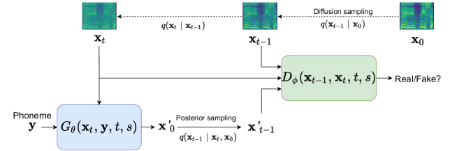
Figure 1: Training process of DiffGAN-TTS.

Another class of generative models called denoising diffusion probabilistic models (DDPMs), or abbreviated as diffusion models, has shown an impressive capability to model complex data distributions. Diffusion models have obtained state-of-the-art results in several important domains, including image synthesis(Ho et al., 2020), audio synthesis(Kong et al., 2021; Chen et al., 2021; Popov et al., 2021), graphs(Niu et al., 2020), and symbolic music generation (Mittal et al., 2021). Typical diffusion models comprise a parameter-free $T$-step Markov chain called the diffusion process, which gradually adds small random noise into the data, and a parameterized $T$-step Markov chain called the denoising process (also known as the reverse process), which removes the added noise as a denoising function. In spite of wide and successful applications of diffusion models in different tasks, sampling from them is not efficient and often requires hundreds or even thousands of denoising steps, making them unsuited for real-time applications. In (Xiao et al., 2021), this slow sampling issue of diffusion models is attributed to the fact that they commonly assume that the denoising distribution can be approximated by Gaussian distributions. This assumption imposes a constraint on typical diffusion models that the denoising step size is sufficiently small and the number of diffusion steps large enough. To use larger denoising step sizes, a conditional GAN is adopted as a non-Gaussian multimodal function to model the denoising distribution (Xiao et al., 2021), leading to much more efficient sampling and, at the same time, competitive sample diversity and fidelity.

This paper introduces DiffGAN-TTS, which is a novel non-AR TTS model based on diffusion models and achieves high-fidelity and efficient TTS. DiffGAN-TTS leverages the powerful modeling capability of diffusion models to address the challenging one-to-many text-to-spectrogram mapping problem. Partially inspired by the denoising diffusion GAN model (Xiao et al., 2021), we model the denoising distribution with an expressive acoustic generator, which is adversarially trained to match the true denoising distribution. DiffGAN-TTS allows large denoising steps at inference, which greatly reduces the number of denoising steps and accelerates sampling. We introduce an active shallow diffusion mechanism into DiffGAN-TTS to further accelerate its sampling process. A two-stage training scheme is designed, where a basic acoustic model trained in stage 1 provides strong prior information for a denoising model trained in stage 2.

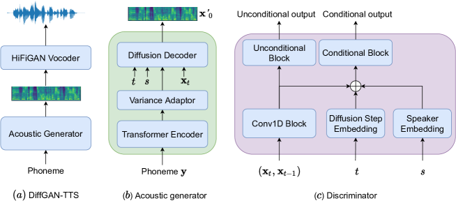
Figure 2: The overall architecture of DiffGAN-TTS.

2 Diffusion Models

Diffusion models usually consist of a parameter-free ${T}$-step Markov chain named the diffusion process and a parameterized $T$-step Markov chain called the reverse process or the denoising process. The diffusion process gradually adds small Gaussian noises into the data until the data structure is totally destroyed at step $T$, while the reverse process learns a denoising function to remove the added noise to restore the data structure.

We define $q(\mathbf{x}_{0})$ as the data distribution on $\mathbb{R}^{L}$, where $L$ is the data dimension, and $q(\mathbf{x}_{T})\sim\mathcal{N}(\mathbf{0},\mathbf{I})$ as the latent variable at step $T$. Let $\mathbf{x}_{t}\in\mathbb{R}^{L}$ for $t=0,1,\cdots,T$ be sequence of variables with the same dimension, where $t$ is the index for diffusion steps. The diffusion process is modeled as a Gaussian transformation chain from data $\mathbf{x}_{0}$ to the latent variable $\mathbf{x}_{T}$ with pre-defined variance schedule $\beta_{1},\cdots,\beta_{T}$:

$$q(\mathbf{x}_{1:T}|\mathbf{x}_{0})=\prod_{t\geq 1}q(\mathbf{x}_{t}|\mathbf{x}_{t-1}),$$ (1)

where $q(\mathbf{x}_{t}|\mathbf{x}_{t-1}):=\mathcal{N}(\mathbf{x}_{t};\sqrt{1-\beta_{t}}\mathbf{x}_{t-1},\beta_{t}\mathbf{I}).$ The reverse or denoising process parameterzied with $\theta$ is defined by:

$$p_{\theta}(\mathbf{x}_{0:T})=p(\mathbf{x}_{T})\prod_{t\geq 1}p_{\theta}(\mathbf{x}_{t-1}|\mathbf{x}_{t}).$$ (2)

The denoising distribution $p_{\theta}(\mathbf{x}_{t-1}|\mathbf{x}_{t})$ is often modeled as a conditional Gaussian distribution as $p_{\theta}(\mathbf{x}_{t-1}|\mathbf{x}_{t}):=\mathcal{N}(\mathbf{x}_{t-1};\mathbf{\mu}_{\theta}(\mathbf{x}_{t}),\sigma_{t}^{2}\mathbf{I})$, where $\mu_{\theta}(\mathbf{x}_{t},t)$ and $\sigma_{t}^{2}\mathbf{I}$ are the mean and variance for the denoising model. Given the parameterized reverse process with the well-learned parameter $\theta$, the sampling process (i.e., the generative process) is to first sample a Gaussian noise $\mathbf{x}_{T}\sim\mathcal{N}(\mathbf{0},\mathbf{I})$, and then iteratively sample $\mathbf{x}_{t-1}\sim p_{\theta}(\mathbf{x}_{t-1}|\mathbf{x}_{t})$ for $t=T,T-1,\cdots,1$ along the reverse process, according to the so-called Langevin dynamics. The $\mathbf{x}_{0}$ is the generated data.

The likelihood $p_{\theta}(\mathbf{x}_{0})=\int p_{\theta}(\mathbf{x}_{0:T})\text{d}\mathbf{x}_{1:T}$ is intractable. Hence, the goal of training is to maximize its evidence lower bound (ELBO$\leq\log p_{\theta}(\mathbf{x}_{0})$), which can be optimized to match the true denoising distribution $q(\mathbf{x}_{t-1}|\mathbf{x}_{t})$ with the parameterized denoising model $p_{\theta}(\mathbf{x}_{t-1}|\mathbf{x}_{t})$ with:

$$\text{ELBO}=\sum_{t\geq 1}\mathbb{E}_{q_{(}{\mathbf{x}_{t}})}[D_{KL}(q(\mathbf{x}_{t-1}|\mathbf{x}_{t})||p_{\theta}(\mathbf{x}_{t-1}|\mathbf{x}_{t})]+c$$ (3)

where $D_{KL}$ denotes the Kullback-Leibler (KL) divergence and $c$ contains constant terms that does not dependent on $\theta$. The KL divergence terms in Eq. 3 are generally intractable due to the unknown true denoising distritbuion $q(\mathbf{x}_{t-1}|\mathbf{x}_{t})$. Therefore, in (Ho et al., 2020) the step size $\beta_{t}$ in the variance schedule is assumed to be small and the number of denoising steps $T$ to be large enough such that both the diffusion and denoising processes have the same functional form (i.e., conditional Gaussian). Based on this, (Ho et al., 2020) shows a certain parameterization, transforming the ELBO optimization problem into a simple regression problem.

3 DiffGAN-TTS

Although DDPMs have demonstrated their capability in modeling complex data distributions, their slow inference speed prevents them from being used in real-time applications. This is due to the two key commonly-made assumptions in DDPMs (Xiao et al., 2021), as alluded to in Section 1: First, the denoising distribution $p_{\theta}(\mathbf{x}_{t-1}|\mathbf{x}_{t})$ is modeled with a Gaussian distribution. Second, the number of denoising steps $T$ is often assumed to be large enough such that $\beta_{t}$ is small. When the denoising step gets larger and the data distribution is non-Gaussian, the true denoising distribution becomes more complex and multimodal, and in such a case, adopting a parameterized Gaussian transformation to approximate the denoising distribution is insufficient for high-quality generation. Conditional GANs have been adopted to model the multimodal denoising distribution in image generation tasks (Xiao et al., 2021). In this section, we show in great detail how we apply this idea to efficient and high-fidelity multi-speaker TTS.

3.1 Acoustic generator and Discriminator

In this work, we focus on the more challenging multi-speaker TTS tasks, which is much harder than single-speaker TTS since acoustic variations are enlarged by data from different speakers. As illustrated in Figure 2$(a)$, DiffGAN-TTS takes phoneme sequence (denoted as $\mathbf{y}$) obtained from a text analysis tool as input to generate intermediate mel-spectrogram features $\mathbf{x}_{0}$ with a multi-speaker acoustic generator and then uses a HiFi-GAN-based neural vocoder (Kong et al., 2020) to produce time-domain waveforms. DDPMs are introduced into the acoustic generator to solve the ill-posed multimodal phoneme-to-mel-spectrogram mapping problem.

The training process of DiffGAN-TTS is illustrated in Figure 1. Our goal is to reduce the number of denoising steps $T$ (e.g., $T\leq 4$) of DiffGAN-TTS such that its inference process is efficient, adequate for real-time speech processing applications without degrading the quality of the generated speech. We focus on discrete-time diffusion models, where denoising steps are large, and use a conditional GAN to model the denoising distribution. DiffTTS-GAN trains a conditional GAN-based acoustic generator $p_{\theta}(\mathbf{x}_{t-1}|\mathbf{x}_{t})$ to approximate the true denoising distribution $q(\mathbf{x}_{t-1}|\mathbf{x}_{t})$ with an adversarial loss that minimizes a divergence $D_{\text{adv}}$ per denoising step:

$$\min_{\theta}\sum_{t\geq 1}\mathbb{E}_{q(\mathbf{x}_{t})}[D_{\text{adv}}(q(\mathbf{x}_{t-1}|\mathbf{x}_{t})||p_{\theta}(\mathbf{x}_{t-1}|\mathbf{x_{t}}))],$$ (4)

where we adopt the least-squares GAN (LS-GAN) training formulation (Mao et al., 2017) to minimize $D_{\text{adv}}$ because of its various successful practices in audio generation domain (Kumar et al., 2019; Kong et al., 2020; Yang et al., 2021; Kim et al., 2021).

Let us denote the speaker-ID as $s$. The discriminator is designed to be diffusion-step-dependent and speaker-aware to aid the generator to achieve high-fidelity multi-speaker speech generation, as illustrated in Figure 2($c$). The discriminator, denoted as $D_{\phi}(\mathbf{x}_{t-1},\mathbf{x}_{t},t,s)$ with learnable parameters $\phi$, is modeled as joint conditional and unconditional (JCU)(Yang et al., 2020, 2021). It not only outputs unconditional logits, but also conditional logits, where diffusion step embedding and speaker embedding are regarded as conditions.

We follow the same scheme in (Xiao et al., 2021) to parameterize the denoising function as an implicit denoising model. Specifically, instead of directly modeling $p_{\theta}(\mathbf{x}_{t-1}|\mathbf{x}_{t})$ by predicting $\mathbf{x}_{t-1}$ from $\mathbf{x}_{t}$, the denoising function is modeled as $p_{\theta}(\mathbf{x}_{t-1}|\mathbf{x}_{t}):=q(\mathbf{x}_{t-1}|\mathbf{x}_{t},\mathbf{x}_{0}=f_{\theta}(\mathbf{x}_{t},t))$, where $\mathbf{x}_{0}$ is predicted from diffused sample $\mathbf{x}_{t}$ using a diffusion function $f_{\theta}(\mathbf{x}_{t},t)$ parameterized with $\theta$. During training, $\mathbf{x}^{\prime}_{t-1}$ is sampled using the posterior distribution $q(\mathbf{x}^{\prime}_{t-1}|\mathbf{x}^{\prime}_{0},\mathbf{x}_{t})$, where $\mathbf{x}^{\prime}_{0}$ is a predicted version of $\mathbf{x}_{0}$. The predicted tuple $(\mathbf{x}^{\prime}_{t-1},\mathbf{x}_{t})$ is then fed into the JCU discriminator to compute the divergence $D_{\text{adv}}$ to the corresponding bonafide counterpart $(\mathbf{x}_{t-1},\mathbf{x}_{t})$. Different from (Xiao et al., 2021), we do not use the latent variable $z\sim\mathcal{N}(\mathbf{0},\mathbf{I})$ as an input to the acoustic generator, since the diffusion decoder takes variance-adapted text encodings (happened in variance adaptor of the acoustic generator) and speaker-ID as auxiliary input. To summarize, the implicit distribution $f_{\theta}(\mathbf{x}_{t},t)$ is modeled with the acoustic generator, denoted as $G_{\theta}(\mathbf{x}_{t},\mathbf{y},t,s)$, which predicts $\mathbf{x}_{0}$ from $\mathbf{x}_{t}$ conditioned on phoneme input $\mathbf{y}$, diffusion step index $t$ and speaker ID $s$.

3.2 Training loss

The discriminator is trained to minimize the loss

$$\begin{split}\mathcal{L}_{D}=\sum_{t\geq 1}\mathbb{E}_{q(\mathbf{x}_{t})q(\mathbf{x}_{t-1}|\mathbf{x}_{t})}[(D_{\phi}(\mathbf{x}_{t-1},\mathbf{x}_{t},t,s)-1)^{2}]\\ +\mathbb{E}_{p_{\theta}(\mathbf{x}_{t-1}|\mathbf{x}_{t})}[D_{\phi}(\mathbf{x}_{t-1},\mathbf{x}_{t},t,s)^{2}].\end{split}$$ (5)

To train the acoustic generator, we also use the feature matching loss $\mathcal{L}_{fm}$, which learns similarity metric to discriminate real and fake data in the feature space (Larsen et al., 2016). $\mathcal{L}_{fm}$ is computed by summing $l_{1}$ distances between every discriminator feature maps of real and generated samples:

where $N$ is the total number of hidden layers in the discriminator. Acoustic reconstruction loss is also used as additional loss to train the acoustic generator following FastSpeech2 (Ren et al., 2021a), as:

$$\begin{split}\mathcal{L}_{recon}=\mathcal{L}_{mel}(\mathbf{x}_{0},\mathbf{x}^{\prime}_{0})+\lambda_{d}\mathcal{L}_{duration}(\mathbf{d},\hat{\mathbf{d}})+\\ \lambda_{p}\mathcal{L}_{pitch}(\mathbf{p},\hat{\mathbf{p}})+\lambda_{e}\mathcal{L}_{energy}(\mathbf{e},\hat{\mathbf{e}}),\end{split}$$ (7)

where $\mathbf{d}$, $\mathbf{p}$ and $\mathbf{e}$ are target duration, pitch and energy, respectively, and $\mathbf{\hat{d}}$, $\mathbf{\hat{p}}$ and $\mathbf{\hat{e}}$ are their corresponding predicted values. $\lambda_{d}$, $\lambda_{p}$ and $\lambda_{e}$ are loss weights, which are all set to be 0.1. $\mathcal{L}_{mel}$ uses MAE loss, while $\mathcal{L}_{duration}$, $\mathcal{L}_{pitch}$ and $\mathcal{L}_{energy}$ use MSE loss. In total, the acoustic generator is trained by minimizing:

$$\mathcal{L}_{G}=\mathcal{L}_{adv}+\mathcal{L}_{recon}+\lambda_{fm}\mathcal{L}_{fm},$$ (8)

where

$$\mathcal{L}_{adv}=\sum_{t\geq 1}\mathbb{E}_{q(\mathbf{x}_{t})}\mathbb{E}_{p_{\theta}(\mathbf{x}_{t-1}|\mathbf{x}_{t})}[(D_{\phi}(\mathbf{x}_{t-1},\mathbf{x}_{t},t,s)-1)^{2}],$$ (9)

and $\lambda_{fm}$ is a dynamically scaled scalar computed as $\lambda_{fm}=\mathcal{L}_{recon}/\mathcal{L}_{fm}$ following (Yang et al., 2021). Detailed training procedure as well as inference procedure is presented in Appendix B.

3.3 Active shallow diffusion mechanism

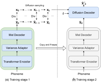
Figure 3: Two-stage training scheme.

In the TTS literature, many acoustic models are trained with a simple loss, such as mean squared error (MSE) loss or mean absolute error (MAE) loss. Acoustic features generated from these acoustic models often suffer from over-smoothing issues due to incorrect uni-modal distribution assumptions on data, leading to non-desired synthesis performance. Nonetheless, the blurry acoustic predictions are not without use. It has been shown that output from acoustic models trained with MSE or MAE loss could provide strong prior knowledge of acoustic features (e.g., coarse harmonic structure), which could be further leveraged by a DDPM to generate refined features, leading to improved synthesis performance(Liu et al., 2021a).

To further accelerate inference of DiffGAN-TTS, we introduce an active shallow diffusion mechanism. As illustrated in Figure 3, a two-stage training scheme is designed. At training stage 1, a basic acoustic model, denoted as $G_{\psi}^{\text{base}}(\mathbf{y},s)$ parameterized with $\psi$, is trained by:

$$\min_{\psi}\sum_{t\geq 0}\mathbb{E}_{q(\mathbf{x}_{t})}[\text{Div}(q_{\text{diff}}^{t}(G^{\text{base}}_{\psi}(\mathbf{y},s)),q_{\text{diff}}^{t}(\mathbf{x}_{0}))],$$ (10)

where $\text{Div}(\cdot,\cdot)$ is a distance function to measure the divergence between the predicted and ground-truth, and $q_{\text{diff}}^{t}(\cdot)$ is the diffusion sampling function at step $t$, e.g., $\mathbf{x}_{t}=q_{\text{diff}}^{t}(\mathbf{x}_{0})$. It’s worthy to note that $q_{\text{diff}}^{0}(\cdot)$ is an identity function. The training objective forces the base acoustic model to actively learn to make the diffused samples from ground-truth acoustic features and those from the predicted indistinguishable. At training stage 2, pre-trained weights of the basic acoustic model are copied to initialize the corresponding weights of the acoustic generator of DiffGAN-TTS and then freeze, as illustrated in Figure 3. The base acoustic model generates coarse mel spectrogram $\hat{\mathbf{x}}_{0}$, which is taken as conditioning by the diffusion decoder. The divergence $D_{\text{adv}}(q(\mathbf{x}_{t-1}|\mathbf{x}_{t})||p_{\theta}(\mathbf{x}_{t-1}|\mathbf{x_{t}}))$ in Eq. 10 is approximated by $D_{\text{adv}}(q(\mathbf{x}_{t-1}|\mathbf{x}_{t})||p_{\theta}(\mathbf{x}_{t-1}|\mathbf{x}_{t},\hat{\mathbf{x}}_{0}))$. Empirically, the diffusion decoder can be regarded as a post filter that conducts “super-resolution” on the coarse prediction produced by the basic acoustic model. We focus on reducing the number of denosing steps to one. During inference, the basic acoustic model first generates a coarse mel spectrogram $\hat{\mathbf{x}}_{0}$, on which a diffused sample at diffusion step 1 is computed (i.e., $\hat{\mathbf{x}}_{1}$). Then DiffGAN-TTS takes $\hat{\mathbf{x}}_{1}$ as prior and runs one denoising step to get the final output. We term this variant as DiffGAN-TTS (two-stage), whose detailed training and inference procedures are presented in Appendix B.

Table 1: Objective and subjective evaluation as well as model efficiency results. SSIM, MCD, $F_{0}$ RMSE, and voice Cosine similarity (Cos. Sim.) are adopted as objective metrics. MOS, as the subjective metric, is presented with 95% confidence intervals. RTFs are estimated on an NVIDIA T4 GPU.

Model	SSIM($\uparrow$)	MCD24($\downarrow$)	F0 RMSE($\downarrow$)	Cos. Sim.($\uparrow$)	#Params.	RTF	MOS($\uparrow$)
GT	-						4.73$\pm$0.07
GT (Mel+HiFi-GAN)	0.823	3.37	37.30	0.907	12.91M	0.0313	4.36$\pm$0.07
FastSpeech 2	0.501	5.97	46.61	0.726	25.54M	0.0058	4.03$\pm$0.08
GANSpeech	0.516	5.27	45.83	0.789	25.54M	0.0058	4.12$\pm$0.11
DiffSpeech	0.498	5.58	48.77	0.736	44.43M	0.2224	4.28$\pm$0.08
DiffGAN-TTS ($T$=1)	0.529	5.08	48.45	0.819	32.81M	0.0069	3.97$\pm$0.10
DiffGAN-TTS ($T$=2)	0.524	5.06	47.24	0.823	32.81M	0.0105	4.01$\pm$0.09
DiffGAN-TTS ($T$=4)	0.532	4.93	45.68	0.806	32.81M	0.0176	4.22$\pm$0.08
DiffGAN-TTS (two-stage)	0.531	5.09	46.26	0.783	42.64M	0.0097	4.17$\pm$0.08

3.4 Model architecture

The transformer encoder in the acoustic generator of DiffGAN-TTS uses the same architecture as that in FastSpeech 2, which consists of 4 feed-forward transformer (FFT) blocks. The hidden size, number of attention heads, kernel size and filter size of the one-dimensional convolution in the FFT block are set as 256, 2, 9 and 1024, respectively. The variance adaptor has the same network structure and hyper-parameters as that in FastSpeech2, which consists of a duration predictor, a pitch predictor and an energy predictor. Differently, the pitch predictor and the energy predictor output phoneme-level fundamental frequency ($F_{0}$) contour and energy contour, respectively, whose labels are obtained by averaging frame-level $F_{0}$ and energy values according to phoneme-audio alignment information obtained from a hidden-Markov-model (HMM)-based forced aligner.

The diffusion decoder in DiffGAN-TTS uses a non-causal WaveNet architecture (Oord et al., 2016) with a slight modification. We use a dilation rate of 1 because we are working with mel spectrograms rather than raw waveforms. With a dilation rate of 1, the diffusion decoder’s receptive field is large enough. The diffusion decoder first performs an one-dimensional (1D) convolutional operation with kernel-size 1 (Conv1x1) on the noisy mel spectrogram $\mathbf{x}_{t}$ before applying the ReLU activation to the output. Diffusion step $t$ is encoded using the same sinusoidal positional encoding as in (Vaswani et al., 2017). The mel spectrogram feature maps are added with the diffusion step embedding, which is then fed into 20 WaveNet residual blocks with a hidden dimension of 256. The transformer encoder’s output is imported into each residual block via separate Conv1x1 layers, whose output is added to the hidden feature maps. Then the gated mechanism introduced in (Oord et al., 2016) is used to further process the feature maps. We add the skip connections from all WaveNet blocks and then process them with two Conv1x1 layers interleaved with a ReLU activation to get the diffusion decoder output. All WaveNet residual blocks have their speaker-IDs transformed into embedding vectors. Appendix A contains additional information.

The JCU discriminator, as depicted in Figure 2($c$), adopts purely convolution networks. The Conv1D block consists of 3 one-dimensional convolutional layers with LeakyReLU (slope=$0.2$) as the activation function. The diffusion step embedding layer is the same as that in the diffusion decoder introduced above. The unconditional block and the conditional block have the same network structure, consisting of two 1D convolutional layers. The channels of convolution are 64, 128, 512, 128, and 1. The kernel sizes are 3, 5, 5, 5, and 3 and the strides are 1, 2, 2, 1, and 1.

The transformer encoder and variance adaptor in the basic acoustic model introduced in Section 3.3 are the same as those in DiffGAN-TTS acoustic generator. The mel decoder is composed of 4 FFT blocks.

4 Experiments

4.1 Data and Preprocessing

We conduct experiments on an internal gender-balanced corpus comprising transcribed speech data from 228 Mandarin Chinese speakers. In total, the corpus has 200 hours of speech data. We randomly split 1024 utterances for validation and another 1024 utterances for testing. Speech samples are all sampled at 24,000 Hz with 16-bit quantization. Mel spectrograms with 80 frequency bins are computed through a short-time Fourier transform (STFT) using a 1024-point window size and a 10 ms frame-shift. We use the PyWorld toolkit to compute $F_{0}$ values from speech signals. Energy features are computed by taking the $l_{2}$-norm of frequency bins in STFT magnitudes.

4.2 Training

We train DiffGAN-TTS models with $T$=1, 2, and 4 using the Adam optimizer (Kingma & Ba, 2015), with $\beta_{1}=0.5$ and $\beta_{2}=0.9$, for both the generator and the discriminator. The detailed computation of the variance schedule is presented in Appendix B. We use an exponential learning rate decay with rate 0.999 for training both the generator and discriminator. Initial learning rate for the generator is $10^{-4}$, while that for the discriminator is $2\times 10^{-4}$. Models are trained using one NVIDIA V100 GPU. The batch size is set to 64, and models are trained for at least 300k steps until losses converge. In the two-stage training scheme, the basic acoustic model is trained 200k steps with the Adam optimizer with $\beta_{1}=0.9$ and $\beta_{2}=0.98$ and follows the same learning rate schedule in (Vaswani et al., 2017). As the distance function, we employ the simple MAE loss.

4.3 Experimental Setup for Comparison

We compare the proposed DiffGAN-TTS model with three strong counterpart models. The first counterpart is the representative non-AR TTS model FastSpeech 2 (Ren et al., 2021a). The second model is the GANSpeech model introduced in (Yang et al., 2021). The third model is the DiffSpeech model presented in (Liu et al., 2021a). We use 60 denoising steps for the best performance on our data.

All compared models use the same acoustic feature setting and the same HiFi-GAN vocoder to ensure fairness. The official implementation (the “config_v1.json” configuration) is used with slight changes. Since we use 24 kHz audio samples and the hop-size for computing the mel spectrogram is 240, we factorize the upsample rate as $240=8\times 5\times 3\times 2$. Moreover, we use the temporal nearest interpolation layer followed by a 1D convolutional layer as the upsampling operation to avoid possible checkerboard artifacts caused by the ”ConvTranspose1d” upsampling layer (Odena et al., 2016).

5 Results

5.1 Objective Evaluation

The quality and voice similarity of generated speech are measured. We conducted an objective evaluation using the structural similarity index measure (SSIM) (Wang et al., 2004), mel-cepstral distortion (MCD)(Kubichek, 1993), $F_{0}$ root mean squared error (RMSE), and voice Cosine similarity. The computation of MCD and $F_{0}$ adopts dynamic time warping (DTW) (dtw, 2007) to align the generated speech and the corresponding ground-truth recording. We use the first 24 coefficients when computing mel cepstrums. For computing voice Cosine similarity, we use a pre-trained speaker classifier to extract embedding vectors (the so-called d-vectors) of a generated sample and its ground-truth counterpart, and then compute the Cosine distance between the two vectors. The results are shown in Table 1. We have the following observations: 1) The four DiffGAN-TTS models achieve the best SSIM, MCD, $F_{0}$ RMSE and voice Cosine similarity. Specifically, the DiffGAN-TTS ($T$=4) model outperforms other compared models in terms of SSIM, MCD, and $F_{0}$ RMSE. This indicates that adopting adversarial training in diffusion models well addresses the one-to-many mapping problem in TTS and is able to achieve high-quality speech synthesis, even when modeling multiple speakers within one model. 2) The best voice Cosine similarity is achieved by the proposed DiffGAN-TTS ($T$=2) model, and meanwhile, DiffGAN-TTS ($T$=1) has the second-highest voice Cosine similarity score. Although the voice Cosine similarity of DiffGAN-TTS ($T$=4) is not the best, it reaches a value of up to 0.806, which is still better than previous TTS models (e.g., FastSpeech 2, GANSpeech and DiffSpeech). Comparing the voice Cosine similarity of DiffGAN-TTS ($T$=1, 2, 4 and two-stage) with that of DiffSpeech, which takes up to 60 diffusion steps at inference, we conjecture that taking more diffusion steps should degrade voice similarity. 3) The DiffGAN-TTS (two-stage) model, which uses the active shallow diffusion mechanism, achieves overall good performance in terms of the four objective metrics. It is noteworthy that DiffGAN-TTS (two-stage) obtains better SSIM and $F_{0}$ RMSE results than DiffGAN-TTS ($T$=1 and $T$=2) and an on-par MCD score, indicating the effectiveness of the proposed active shallow diffusion mechanism.

5.2 Subjective Evaluation

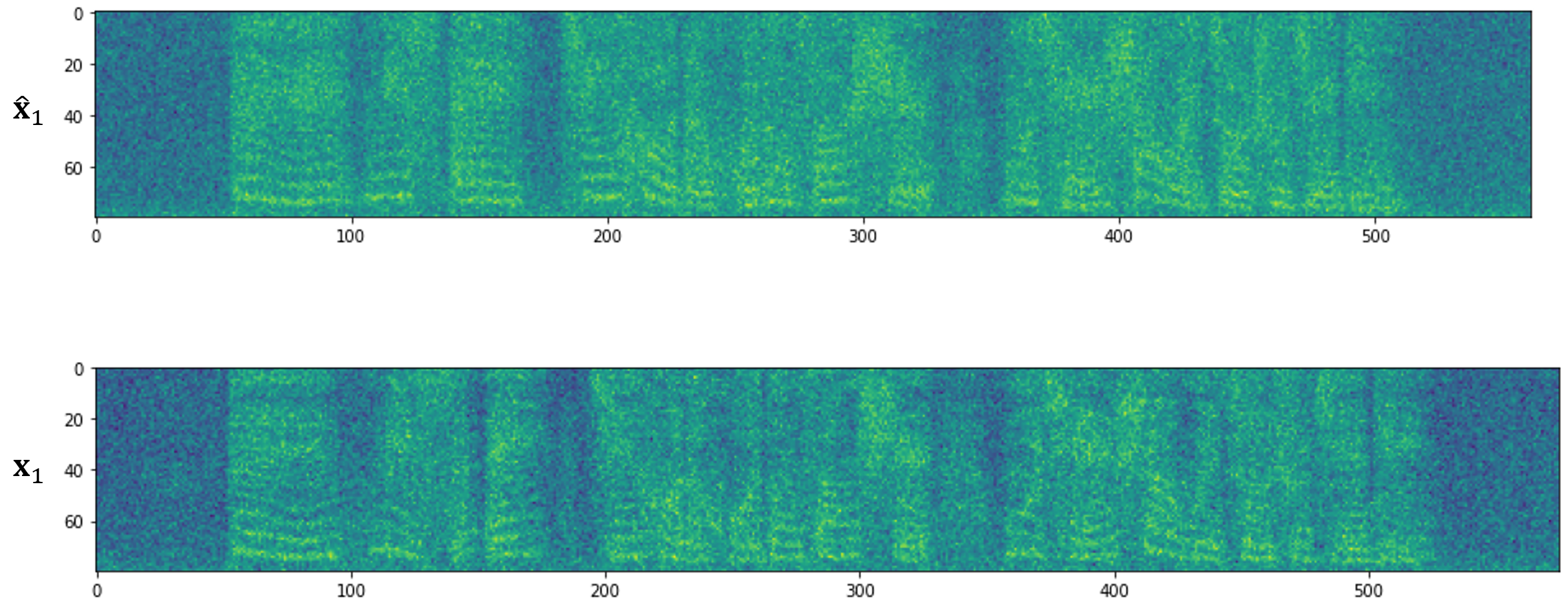
Figure 4: Diffused samples at step 1. $\hat{\mathbf{x}}_{0}$: diffused sample from predicted mel spectrogram. $\mathbf{x}_{0}$: diffused sample from ground-truth mel spectrogram.

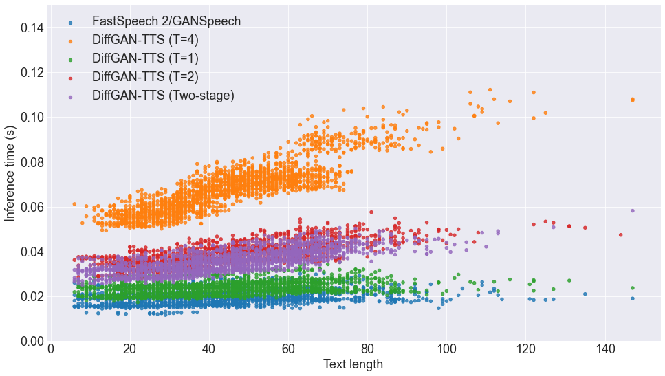
Figure 5: Inference time (second) v.s. text length (given in number of phonemes).

We conduct crowd-sourced mean opinion score (MOS) tests to evaluate the quality of the generated speech perceptually. We keep the text content consistent among different models to exclude other interference factors, only examining the audio quality. Each audio sample is rated by at least 20 testers, who are asked to estimate the quality of synthesized speech on a nine-point Likert scale, with the lowest and highest scores being 1 (“Bad”) and 5 (“Excellent”), and with an increment step of 0.5. A subset of the audio samples is available online . The evaluation results are shown in the last column of Table 1. We observe that the DiffSpeech model ($T$=60) outperforms other models in spite of its sub-optimal performance in objective measurement. This indicates that diffusion models may take a trade-off between model capacity and inference speed and be able to obtain higher quality with a larger number of denoising steps. Overall, the DiffGAN-TTS family achieves good MOS results, with DiffGAN-TTS ($T$=4) obtaining the second-highest MOS (i.e., 4.22). We can see that DiffGAN-TTS (two-stage) achieves a MOS of 4.17, which is significantly better than DiffGAN-TTS ($T$=1 and 2). This verifies the two-stage training scheme and the active shallow diffusion mechanism introduced in Section 3.3. A visualization of taking one diffusion step on a predicted mel spectrogram by DiffGAN-TTS (two-stage) at training stage 1 (denoted as $\hat{\mathbf{x}}_{1}$) and its corresponding ground truth (denoted as $\mathbf{x}_{1}$) is shown in Figure 4. We see that $\hat{\mathbf{x}}_{1}$ has a similar harmonic structure to $\mathbf{x}_{1}$, which inspires us to use the former as a strong prior for the latter.

Table 2: Objective metrics for ablation study.

Model	SSIM	MCD24	F0 RMSE	Cos. Sim.
DiffGAN-TTS	0.532	4.93	45.68	0.806
($T$=4)
$-\mathcal{L}_{fm}$	0.529	5.23	47.99	0.782
$-\mathcal{L}_{mel}$	0.492	5.86	48.97	0.710
$-\mathcal{L}_{fm}-\mathcal{L}_{mel}$	[Does not train]
$+$ latent $\mathbf{z}$	0.517	5.10	46.68	0.794

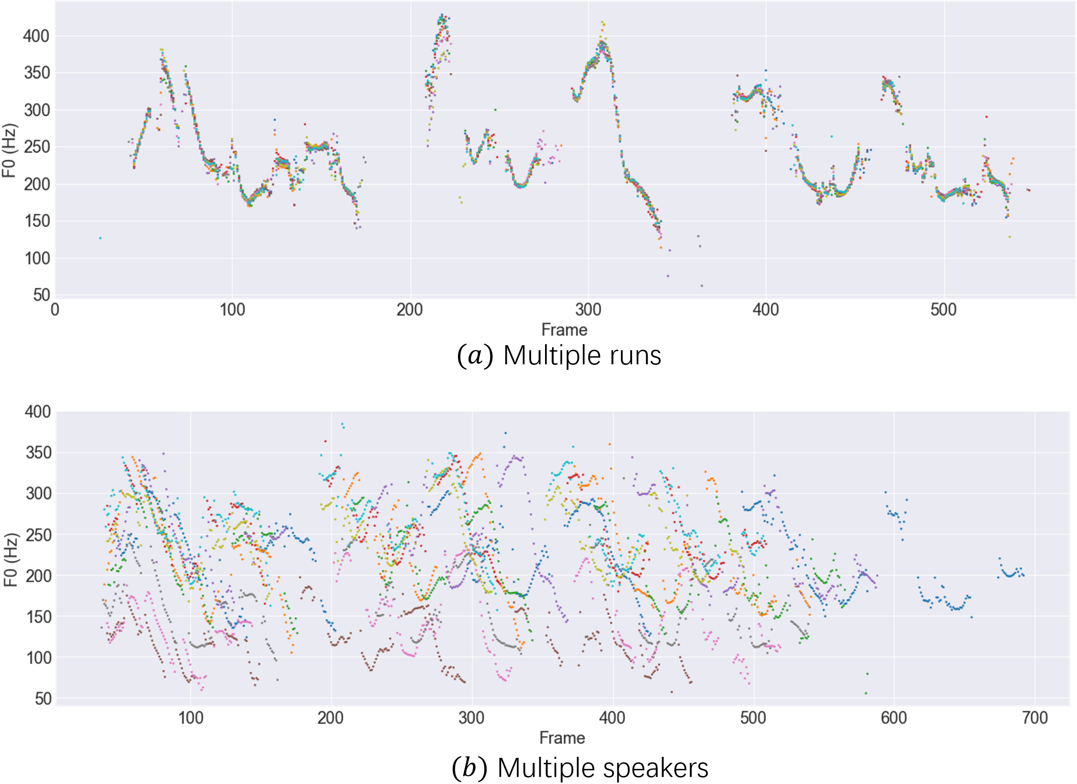
Figure 6: Pitch tracks. ($a$): $F_{0}$ contours of 10 different runs with the same text input and speaker conditioning. ($b$): $F_{0}$ contours of 10 different speakers with the same text input.

5.3 Synthesis Speed

We assess the synthesis speed of mel spectrograms in terms of the Real-Time factor (RTF), indicating how many seconds it takes to generate one second of audio, on an NVIDIA T4 GPU and the number of model parameters. The efficiency information for all models is presented in Table 1. We also evaluate the scaling performance (inference time v.s. text length), as illustrated in Figure 5, where DiffSpeech is not depicted since its inference is too slow, making the plots of other models indistinguishable. It shows that DiffGAN-TTS ($T$=1) has similar scaling performance to FastSpeech 2 and other models have satisfactory scaling performance.

5.4 Ablation studies

We conducted ablation studies in DiffGAN-TTS ($T$=4) to demonstrate the effectiveness of the use of mel loss $\mathcal{L}_{mel}$ and feature matching loss $\mathcal{L}_{fm}$ introduced in Section 3.2, as well as the exclusion of modeling a latent variable $\mathbf{z}$ in the diffusion decoder. Details of how to use the latent variable are presented in Appendix A. Objective metrics are computed for these ablations. The results are shown in Table 2. The model without using $\mathcal{L}_{mel}$ and $\mathcal{L}_{fm}$ does not train at all, which demonstrates that an adversarial loss alone is not sufficient for training a multi-speaker DiffGAN-TTS model. When comparing the model without $\mathcal{L}_{fm}$ to that without $\mathcal{L}_{mel}$, we observe that mel loss is more important than feature matching loss to successfully train a DiffGAN-TTS model. Adding a latent variable into the model makes all four metrics degrade more or less, indicating that the variance adaptor and speaker conditioning manage to model acoustic variations.

5.5 Synthesis Variation

Unlike the FastSpeech 2 and GANSpeech models, whose output is uniquely determined by the input text and speaker conditioning at inference, DiffGAN-TTS takes sampling processes at denoising steps and can inject some variations into the generated speech. To demonstrate this, we run a DiffGAN-TTS ($T$=4) model 10 times for a particular input text and speaker and compute the $F_{0}$ contours of the generated speech samples. We visualize in Figure 6($a$) and observe that DiffGAN-TTS generates speech with diverse pitches. We also generate speech samples for 10 speakers with the same text input, whose $F_{0}$ contours are visualized in Figure 6($b$), demonstrating that DiffGAN-TTS expresses very different prosody patterns for each speaker.

6 Related Work

The Diffusion model is a family of generative models with the capacity to model complex data distribution and has attracted a lot of research attention in recent years. Two streams of efforts have pushed research on diffusion models forward. One research stream is on score matching models (Hyvärinen, 2005), where the problem of data density estimation is simplified into a score matching problem, i.e., estimating the gradient of the data distribution probabilistic density. The other stream is research on denoising diffusion probabilistic models (DDPMs) (Sohl-Dickstein et al., 2015), where a diffusion Markov chain is adopted to add noise to the data structure and another Markov chain-based reverse process is used to generate data from noise. Lately, progress has been made in these two streams. The diffusion models have been shown to be able to generate high-quality images (Ho et al., 2020). Afterward, DDPMs achieve high-quality audio generation (Kong et al., 2021; Chen et al., 2021) using the same parameterization introduced in (Ho et al., 2020). On the other hand, score matching models have also been proven to generate high-resolution images by adopting a neural network to estimate the log gradient of data density. Slightly later, (Song et al., 2021) generalizes and improves previous work in score matching models through the lens of stochastic differential equations (SDEs) and shows that DDPMs and score matching models are special cases under this unified framework. In spite of wide and successful applications of diffusion models in different tasks, sampling from them is not efficient and often requires hundreds or even thousands of denoising steps, making them unsuited for real-time applications.

This work is inspired partially by (Xiao et al., 2021), which applies diffusion denoising GANs to accelerate inference in DDPMs for image synthesis, whereas we focus on high-fidelity and efficient text-to-speech (TTS) synthesis. Furthermore, we develop a new model architecture and employ new losses to make the model suitable for TTS tasks that cannot be accomplished naturally. The two-stage version of DiffGAN-TTS is closely related to DiffSpeech (Liu et al., 2021a), which introduces a shallow diffusion scheme by training a boundary prediction to find the starting diffusion step at inference. Our work is much different: 1) We train the model to actively fuse the diffusion processes starting from the ground-truth mel spectrogram and the coarse mel spectrogram produced by a basic acoustic model. 2) Our model is adversarial trained and has a much faster inference speed than DiffSpeech. 3) We concentrate on the more difficult multi-speaker TTS tasks, whereas DiffSpeech concentrates on single-speaker TTS tasks. 4) Our model uses coarse model predictions as conditioning in the diffusion module, whereas DiffSpeech uses text encodings.

7 Conclusion

In this work, we have presented DiffGAN-TTS, a novel diffusion model-based non-AR TTS model able to achieve high-fidelity and efficient speech synthesis. DiffGAN-TTS adopts an expressive model as a denoising function to approximate the true denoising distribution with adversarial training. Large denoising steps are allowed in DiffGAN-TTS, leading to faster inference. We show with challenging multi-speaker TTS experiments that DiffGAN-TTS is able to generate high-fidelity speech samples with only four denoising steps. To further accelerate its inference process, we propose an active shallow diffusion mechanism and devise a two-stage training scheme to fully leverage prior knowledge from a basic acoustic model. Experiments show that DiffGAN-TTS is able to achieve high TTS performance with only one denoising step. We hope that DiffGAN-TTS will be used in many speech processing applications, especially those requiring real-time speech generation, to enjoy the powerful modeling capacity of diffusion models. We also want to point out that even though the proposed model achieves decent TTS, it is still within the cascade of an acoustic model with a neural vocoder paradigm. Extending the model to support end-to-end text-to-waveform generation could be a possible direction for a shorter TTS pipeline and even better synthesis performance.

Appendix A Model details

In this section, we present model details of the diffusion decoder in DiffGAN-TTS and the one in the ablation model taking an extra latent variable $\mathbf{z}$ as input (introduced in Section 5.4). The diffusion decoder has structure based on the residual block introduced in WaveNet (Oord et al., 2016). Differently, we make the model non-causal. Figure 7($a$) shows the diffusion decoder used in DiffGAN-TTS ($T$=1, 2 and 4) and as well as DiffGAN-TTS (two-stage). In the figure, FC represents fully-connected layer, and Swish represents the swish activation function (Ramachandran et al., 2018). Figure 7($b$) shows the diffusion decoder where we inject a latent variable $\mathbf{z}\sim\mathcal{N}(\mathbf{0},\mathbf{I})$ as input. Inspired by StyleGAN (Karras et al., 2019) and following (Xiao et al., 2021), the latent variable $\mathbf{z}$ is first transformed by a mapping network, which is simply a fully-connected layer, into an embedding vector, denoted as $\mathbf{w}$. In each residual block, we incorporated the latent variable with adaptive layer normalization (AdaLN) layers. Specifically, a fully-connected layer is applied to convert $\mathbf{w}$ into scale $\mathbf{\gamma}$ and shift $\mathbf{\beta}$ features in each residual block. And then in each AdaLN layer, mean-variance normalization is first conducted on the residual output, and then we use $\mathbf{\gamma}$ and $\mathbf{\beta}$ to modulate the normalized feature $\mathbf{h}_{norm}$ as $\mathbf{h}_{norm}*\mathbf{\gamma}+\mathbf{\beta}$.

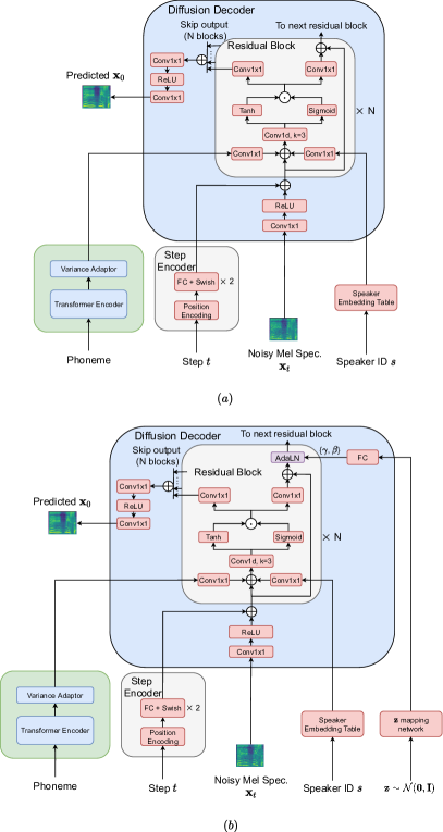
Figure 7: Model details: ($a$) Network structure of the diffusion decoder in DiffGAN-TTS models. ($b$) Network structure of the diffusion decoder modeling an extra latent variable $\mathbf{z}\sim\mathcal{N}(\mathbf{0},\mathbf{I})$.

Appendix B Training and inference algorithms

B.1 The Gaussian posterior

In this section, we include a derivation for the Gaussian posterior distribution presented in (Ho et al., 2020) for completeness. Given a data point sampled from a real distribution $\mathbf{x}_{0}\sim q(\mathbf{x})$, consider the diffusion process as a Markov chain as:

$$q(\mathbf{x}_{1:T}|\mathbf{x}_{0})=\prod_{t\geq 1}q(\mathbf{x}_{t}|\mathbf{x}_{t-1}),\quad q(\mathbf{x}_{t}|\mathbf{x}_{t-1}):=\mathcal{N}(\mathbf{x}_{t};\sqrt{1-\beta_{t}}\mathbf{x}_{t-1},\beta_{t}\mathbf{I}).$$ (11)

Letting $\alpha_{t}=1-\beta_{t}$ and $\bar{\alpha}_{t}=\prod_{i=1}^{t}\alpha_{i}$, a nice property of the diffusion process is that we can sample $\mathbf{x}_{t}$ at any diffusion step $t$ in a closed form (a detailed derivation is given in Appendix A in (Kong et al., 2021)), as:

$$q(\mathbf{x}_{t}|\mathbf{x}_{0})=\mathcal{N}(\mathbf{x}_{t};\sqrt{\bar{\alpha}_{t}}\mathbf{x}_{0},(1-\bar{\alpha}_{t})\mathbf{I}).$$ (12)

By Bayes’ rule and Markov chain property, the reverse conditional probability is tractable when conditioned on $\mathbf{x}_{0}$:

$$\begin{split}q(\mathbf{x}_{t-1}|\mathbf{x}_{t},\mathbf{x}_{0})&=q(\mathbf{x}_{t}|\mathbf{x}_{t-1},\mathbf{x}_{0})\frac{q(\mathbf{x}_{t-1}|\mathbf{x}_{0})}{q(\mathbf{x}_{t}|\mathbf{x}_{0})}\\ &=\frac{q(\mathbf{x}_{t}|\mathbf{x}_{t-1})q(\mathbf{x}_{t-1}|\mathbf{x}_{0})}{q(\mathbf{x}_{t}|\mathbf{x}_{0})}\\ &=\frac{\mathcal{N}(\mathbf{x}_{t};\sqrt{\alpha_{t}}\mathbf{x}_{t-1},\beta_{t}\mathbf{I})\mathcal{N}(\mathbf{x}_{t-1};\sqrt{\bar{\alpha}_{t}}\mathbf{x}_{0},(1-\bar{\alpha}_{t-1})\mathbf{I})}{\mathcal{N}(\mathbf{x}_{t};\sqrt{\bar{\alpha}_{t}}\mathbf{x}_{0},(1-\bar{\alpha}_{t})\mathbf{I})}\\ &\propto\exp{(-\frac{1}{2}(\frac{(\mathbf{x}_{t}-\sqrt{\alpha_{t}}\mathbf{x}_{t-1})^{2}}{\beta_{t}}+\frac{(\mathbf{x}_{t-1}-\sqrt{\bar{\alpha}_{t-1}}\mathbf{x}_{0})^{2}}{1-\sqrt{\bar{\alpha}_{t-1}}}-\frac{(\mathbf{x}_{t}-\sqrt{\bar{\alpha}_{t}}\mathbf{x}_{0})^{2}}{1-\sqrt{\bar{\alpha}_{t}}}))}\\ &=\exp{(-\frac{1}{2}((\frac{\alpha_{t}}{\beta_{t}}+\frac{1}{1-\bar{\alpha}_{t-1}})\mathbf{x}_{t-1}^{2})-(\frac{2\sqrt{\alpha_{t}}}{\beta_{t}}\mathbf{x}_{t}+\frac{2\sqrt{\bar{\alpha}_{t}}}{1-\sqrt{\bar{\alpha}_{t}}}\mathbf{x}_{0})\mathbf{x}_{t-1}+C(\mathbf{x}_{t},\mathbf{x}_{0}))},\end{split}$$ (13)

where $C(\mathbf{x}_{t},\mathbf{x}_{0})$ is not involving $\mathbf{x}_{t-1}$. From the functional form in Eq. 13 and some derivations, we observe that the posterior $q(\mathbf{x}_{t-1}|\mathbf{x}_{t},\mathbf{x}_{0})$ is a Gaussian distribution, which can be written as:

$$q(\mathbf{x}_{t-1}|\mathbf{x}_{t},\mathbf{x}_{0})=\mathcal{N}(\mathbf{x}_{t-1};\tilde{\mathbf{\mu}}_{t}(\mathbf{x}_{t},\mathbf{x}_{0}),\tilde{\beta}_{t}\mathbf{I})$$ (14)

with mean $\tilde{\mathbf{\mu}}_{t}(\mathbf{x}_{t},\mathbf{x}_{0})$ and variance $\tilde{\beta}_{t}$ having the forms of:

$$\tilde{\mathbf{\mu}}_{t}(\mathbf{x}_{t},\mathbf{x}_{0})=\frac{\sqrt{\bar{\alpha}_{t-1}}\beta_{t}}{1-\bar{\alpha}_{t}}\mathbf{x}_{0}+\frac{\sqrt{\alpha_{t}}(1-\bar{\alpha}_{t-1})}{1-\bar{\alpha}_{t}}\mathbf{x}_{t}\quad\text{and}\quad\tilde{\beta}_{t}=\frac{1-\bar{\alpha}_{t-1}}{1-\bar{\alpha}_{t}}\beta_{t}.$$ (15)

B.2 Variance schedule

We use the discretization of the continuous-time extension of the diffusion process in Eq. 12 with the variance preserving (VP) SDE (Song et al., 2021) to compute the variance schedule $\beta_{1},\cdots,\beta_{T}$. Specifically, for $t\in\{1,\cdots,T\}$, we compute $\beta_{t}$ as:

$$\beta_{t}=1-\exp(-\frac{\beta_{\text{min}}}{T}-0.5(\beta_{\text{max}}-\beta_{\text{min}})\frac{2t-1}{T^{2}}),$$ (16)

where we set the constants as $\beta_{\text{min}}=0.1$ and $\beta_{\text{min}}=40$ in all experiments.

B.3 Training algorithm of DiffGAN-TTS

The training procedures of the DiffGAN-TTS models with $T$=1, 2 and 4 are the same across our experiments. We summarize the algorithm in Algorithm 1.

B.4 Inference algorithm of DiffGAN-TTS

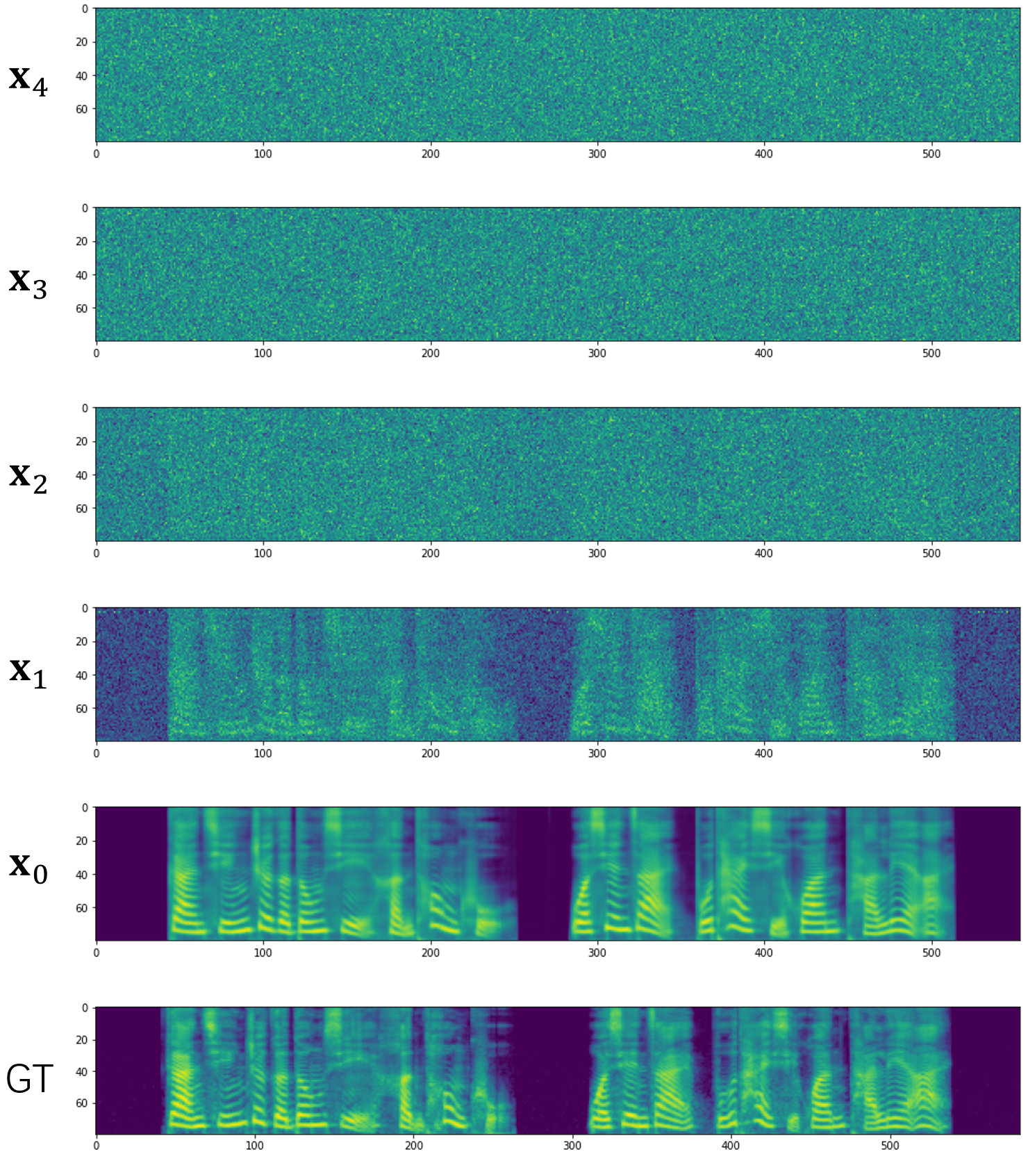
Figure 8: A visualization of the denoising steps in DiffGAN-TTS ($T$=4) at inference. “GT” represents the ground-truth mel spectrogram.

The inference procedures of the DiffGAN-TTS models with $T$=1, 2 and 4 are the same across our experiments. We summarize the algorithm in Algorithm 2. We visualize the denoising steps of the DiffGAN-TTS ($T$=4) model in Figure 8.

B.5 Training algorithm of DiffGAN-TTS with active shallow diffusion

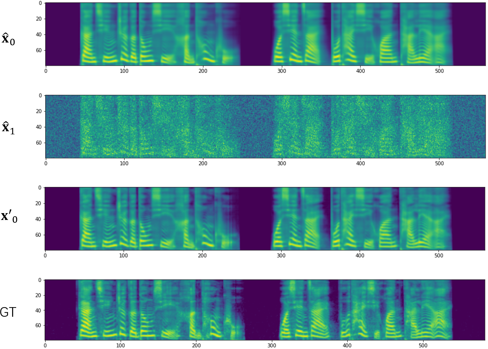
Figure 9: A visualization of the denoising steps in DiffGAN-TTS (two-stage) as inference, which uses the active shallow diffusion mechanism. “GT” represents the ground-truth mel spectrogram.

The training procedures of the DiffGAN-TTS model with active shallow diffusion, i.e., DiffGAN-TTS (two-stage), is summarized in Algorithm 3. We visualize the denoising steps of the DiffGAN-TTS (two-stage) model in Figure 9.

B.6 Inference algorithm of DiffGAN-TTS with active shallow diffusion

The inference procedures of the DiffGAN-TTS model with active shallow diffusion, i.e., DiffGAN-TTS (two-stage), is summarized in Algorithm 4.

Algorithm 1 Training procedure of DiffGAN-TTS

Input: The acoustic generator $G_{\theta}$ with parameters $\theta$. The discriminator $D_{\phi}$ with parameter $\phi$. A pre-calculated variance schedule $\beta_{1},\cdots,\beta_{T}$ with $T$ diffusion steps. The training set $\mathcal{D}_{train}=\{(\mathbf{x}_{0},\mathbf{y},\mathbf{s},\mathbf{d},\mathbf{p},\mathbf{e})_{i}\}_{i=1}^{N}$ with $N$ data points.

1:  Initialize parameters $\theta$ and $\phi$;

2:  while model not converge do

3:     Sample $M$ data points from $\mathcal{D}_{train}$ to form a mini-batch $\mathcal{S}=\{(\mathbf{x}_{0},\mathbf{y},\mathbf{s},\mathbf{d},\mathbf{p},\mathbf{e})_{i}\}_{j=1}^{M}$;

4:     for data point in $\mathcal{S}$ do

5:        Uniformly sample $t$ from $[0,\cdots,T]$;

6:        Sample $\mathbf{x}_{t}$ and $\mathbf{x}_{t-1}$ given $\mathbf{x}_{0}$ according to Eq.12;

7:        Add $t$, $\mathbf{x}_{t}$ and $\mathbf{x}_{t-1}$ to current data point;

8:     end for

9:     Step I: train the discriminator

10:     Forward-propagate $\mathcal{S}$ to $G_{\theta}$ to obtain output $\mathcal{O}=\{(\mathbf{x}^{\prime}_{0},\hat{\mathbf{d}},\hat{\mathbf{p}},\hat{\mathbf{e}})_{i}\}_{j=1}^{M}$;

11:     Sample the posterior $\mathbf{x}^{\prime}_{t-1}$ for each $\mathbf{x}^{\prime}_{0}$ in $\mathcal{O}$ by Eq. 14;

12:     Compute $\mathcal{L}_{D}$ by Eq. 5;

13:     Do back-propagation with $\mathcal{L}_{D}$ and update $\phi$ one step with gradient descent;

14:     Step II: train the acoustic generator

15:     Compute $\mathcal{L}_{G}$ by Eq. 8;

16:     Do back-propagation with $\mathcal{L}_{G}$ and update $\theta$ one step with gradient descent;

17:  end while

18:  Return $G_{\theta}$;

Algorithm 2 Inference procedure of DiffGAN-TTS

Input: A trained acoustic generator $G_{\theta}$ and one testing sample $(\mathbf{y},s)$.

1:  Sample $\mathbf{x}_{T}\sim\mathcal{N}(\mathbf{0},\mathbf{I})$;

2:  $\mathbf{x}_{t}\leftarrow\mathbf{x}_{T}$;

3:  for $t=T,T-1,...,1$ do

4:     Forward-propagate $(\mathbf{x}_{t},\mathbf{y},s,t)$ to $G_{\theta}$ to calculate $\mathbf{x}^{\prime}_{0}$;

5:     Sample $\mathbf{x}^{\prime}_{t-1}$ given $\mathbf{x}^{\prime}_{0}$ and $\mathbf{x}_{t}$ by Eq. 14;

6:     $\mathbf{x}_{t}\leftarrow\mathbf{x}^{\prime}_{t-1}$;

7:  end for

8:  Return $\mathbf{x}_{t}$;

Algorithm 3 Training procedure of DiffGAN-TTS with active shallow diffusion

Input: The basic acoustic model $G_{\psi}^{\text{base}}$ with parameters $\psi$. The acoustic generator $G_{\theta}$ with parameters $\theta$. The discriminator $D_{\phi}$ with parameter $\phi$. A pre-calculated variance schedule $\beta_{1},\cdots,\beta_{T}$ with $T$ diffusion steps. The training set $\mathcal{D}_{train}=\{(\mathbf{x}_{0},\mathbf{y},\mathbf{s},\mathbf{d},\mathbf{p},\mathbf{e})_{i}\}_{i=1}^{N}$ with $N$ data points. Number of basic acoustic model training iterations $N_{\text{iter}}$.

1:  Initialize parameters $\psi$, $\theta$ and $\phi$;

2:  Stage 1: train the basic acoustic model;

3:  for $i=1,2,...,N_{\text{iter}}$ do

4:     Sample $M$ data points from $\mathcal{D}_{train}$ to form a mini-batch $\mathcal{S}=\{(\mathbf{x}_{0},\mathbf{y},\mathbf{s},\mathbf{d},\mathbf{p},\mathbf{e})_{i}\}_{j=1}^{M}$;

5:     Forward-propagate $\mathcal{S}$ to $G_{\psi}^{\text{base}}$ to obtain output $\mathcal{O}=\{(\hat{\mathbf{x}}_{0},\hat{\mathbf{d}},\hat{\mathbf{p}},\hat{\mathbf{e}})_{i}\}_{j=1}^{M}$;

6:     Compute reconstruction loss $\mathcal{L}_{recon}$ by Eq. 7;

7:     Do back-propagation with $\mathcal{L}_{recon}$ and update $\psi$ one step with gradient descent;

8:  end for

9:  Stage 2: train the diffusion encoder in $G_{\theta}$;

10:  Initialize partial weights in $\theta$ with $\psi$ as introduced in Section 3.3;

11:  while model not converge do

12:     Sample $M$ data points from $\mathcal{D}_{train}$ to form a mini-batch $\mathcal{S}=\{(\mathbf{x}_{0},\mathbf{y},\mathbf{s},\mathbf{d},\mathbf{p},\mathbf{e})_{i}\}_{j=1}^{M}$;

13:     for data point in $\mathcal{S}$ do

14:        Uniformly sample $t$ from $[0,\cdots,T]$;

15:        Sample $\mathbf{x}_{t}$ and $\mathbf{x}_{t-1}$ given $\mathbf{x}_{0}$ according to Eq.12;

16:        Add $t$, $\mathbf{x}_{t}$ and $\mathbf{x}_{t-1}$ to current data point;

17:     end for

18:     Step I: train the discriminator

19:     Forward-propagate $\mathcal{S}$ to $G_{\theta}$ to obtain output $\mathcal{O}=\{(\mathbf{x}^{\prime}_{0},\hat{\mathbf{d}},\hat{\mathbf{p}},\hat{\mathbf{e}})_{i}\}_{j=1}^{M}$;

20:     Sample the posterior $\mathbf{x}^{\prime}_{t-1}$ for each $\mathbf{x}^{\prime}_{0}$ in $\mathcal{O}$ by Eq. 14;

21:     Compute $\mathcal{L}_{D}$ by Eq. 5;

22:     Do back-propagation with $\mathcal{L}_{D}$ and update $\phi$ one step with gradient descent;

23:     Step II: train the acoustic generator

24:     Compute $\mathcal{L}_{G}$ by Eq. 8;

25:     Do back-propagation with $\mathcal{L}_{G}$ and update $\theta$ one step with gradient descent;

26:  end while

27:  Return $G_{\theta}$;

Algorithm 4 Inference procedure of DiffGAN-TTS with active shallow diffusion using one denoising step

Input: A trained acoustic generator $G_{\theta}$ and one testing sample $(\mathbf{y},s)$.

1:  Forward $(\mathbf{y},s)$ through transformer encoder, variance adaptor and mel decoder to obtain coarse prediction $\hat{\mathbf{x}}_{0}$;

2:  Sample $\hat{\mathbf{x}}_{1}$ conditioning on $\hat{\mathbf{x}}_{0}$ by Eq. 12;

3:  Forward-propagate $(\hat{\mathbf{x}}_{1},y,s,t=1)$ to the diffusion decoder in $G_{\theta}$ to calculate $\mathbf{x}^{\prime}_{0}$;

4:  Return $\mathbf{x}^{\prime}_{0}$;

References

- dtw (2007) Dynamic Time Warping, pp. 69–84. Springer Berlin Heidelberg, Berlin, Heidelberg, 2007. ISBN 978-3-540-74048-3. doi: 10.1007/978-3-540-74048-3˙4. URL https://doi.org/10.1007/978-3-540-74048-3_4.
- Badlani et al. (2021) Badlani, R., Łancucki, A., Shih, K. J., Valle, R., Ping, W., and Catanzaro, B. One tts alignment to rule them all. arXiv preprint arXiv:2108.10447, 2021.
- Chen et al. (2021) Chen, N., Zhang, Y., Zen, H., Weiss, R. J., Norouzi, M., and Chan, W. Wavegrad: Estimating gradients for waveform generation. In International Conference on Learning Representations, 2021. URL https://openreview.net/forum?id=NsMLjcFaO8O.
- Donahue et al. (2021) Donahue, J., Dieleman, S., Binkowski, M., Elsen, E., and Simonyan, K. End-to-end adversarial text-to-speech. In International Conference on Learning Representations, 2021. URL https://openreview.net/forum?id=rsf1z-JSj87.
- Elias et al. (2021) Elias, I., Zen, H., Shen, J., Zhang, Y., Jia, Y., Weiss, R. J., and Wu, Y. Parallel tacotron: Non-autoregressive and controllable tts. In ICASSP 2021-2021 IEEE International Conference on Acoustics, Speech and Signal Processing (ICASSP), pp. 5709–5713. IEEE, 2021.
- Gibiansky et al. (2017) Gibiansky, A., Arik, S., Diamos, G., Miller, J., Peng, K., Ping, W., Raiman, J., and Zhou, Y. Deep voice 2: Multi-speaker neural text-to-speech. Advances in neural information processing systems, 30, 2017.
- Ho et al. (2020) Ho, J., Jain, A., and Abbeel, P. Denoising diffusion probabilistic models. In Larochelle, H., Ranzato, M., Hadsell, R., Balcan, M. F., and Lin, H. (eds.), Advances in Neural Information Processing Systems, volume 33, pp. 6840–6851. Curran Associates, Inc., 2020. URL https://proceedings.neurips.cc/paper/2020/file/4c5bcfec8584af0d967f1ab10179ca4b-Paper.pdf.
- Hyvärinen (2005) Hyvärinen, A. Estimation of non-normalized statistical models by score matching. Journal of Machine Learning Research, 6(24):695–709, 2005. URL http://jmlr.org/papers/v6/hyvarinen05a.html.
- Karras et al. (2019) Karras, T., Laine, S., and Aila, T. A style-based generator architecture for generative adversarial networks. In Proceedings of the IEEE/CVF Conference on Computer Vision and Pattern Recognition, pp. 4401–4410, 2019.
- Kim et al. (2020) Kim, J., Kim, S., Kong, J., and Yoon, S. Glow-tts: A generative flow for text-to-speech via monotonic alignment search. In Larochelle, H., Ranzato, M., Hadsell, R., Balcan, M. F., and Lin, H. (eds.), Advances in Neural Information Processing Systems, volume 33, pp. 8067–8077. Curran Associates, Inc., 2020. URL https://proceedings.neurips.cc/paper/2020/file/5c3b99e8f92532e5ad1556e53ceea00c-Paper.pdf.
- Kim et al. (2021) Kim, J., Kong, J., and Son, J. Conditional variational autoencoder with adversarial learning for end-to-end text-to-speech. In Meila, M. and Zhang, T. (eds.), Proceedings of the 38th International Conference on Machine Learning, volume 139 of Proceedings of Machine Learning Research, pp. 5530–5540. PMLR, 18–24 Jul 2021. URL https://proceedings.mlr.press/v139/kim21f.html.
- Kingma & Ba (2015) Kingma, D. P. and Ba, J. Adam: A method for stochastic optimization. ICLR, 2015.
- Kong et al. (2020) Kong, J., Kim, J., and Bae, J. Hifi-gan: Generative adversarial networks for efficient and high fidelity speech synthesis. In Larochelle, H., Ranzato, M., Hadsell, R., Balcan, M. F., and Lin, H. (eds.), Advances in Neural Information Processing Systems, volume 33, pp. 17022–17033. Curran Associates, Inc., 2020. URL https://proceedings.neurips.cc/paper/2020/file/c5d736809766d46260d816d8dbc9eb44-Paper.pdf.
- Kong et al. (2021) Kong, Z., Ping, W., Huang, J., Zhao, K., and Catanzaro, B. Diffwave: A versatile diffusion model for audio synthesis. In International Conference on Learning Representations, 2021. URL https://openreview.net/forum?id=a-xFK8Ymz5J.
- Kubichek (1993) Kubichek, R. Mel-cepstral distance measure for objective speech quality assessment. In Proceedings of IEEE Pacific Rim Conference on Communications Computers and Signal Processing, volume 1, pp. 125–128 vol.1, 1993. doi: 10.1109/PACRIM.1993.407206.
- Kumar et al. (2019) Kumar, K., Kumar, R., de Boissiere, T., Gestin, L., Teoh, W. Z., Sotelo, J., de Brébisson, A., Bengio, Y., and Courville, A. C. Melgan: Generative adversarial networks for conditional waveform synthesis. In Wallach, H., Larochelle, H., Beygelzimer, A., d'Alché-Buc, F., Fox, E., and Garnett, R. (eds.), Advances in Neural Information Processing Systems, volume 32. Curran Associates, Inc., 2019. URL https://proceedings.neurips.cc/paper/2019/file/6804c9bca0a615bdb9374d00a9fcba59-Paper.pdf.
- Larsen et al. (2016) Larsen, A. B. L., Sønderby, S. K., Larochelle, H., and Winther, O. Autoencoding beyond pixels using a learned similarity metric. In International conference on machine learning, pp. 1558–1566. PMLR, 2016.
- Lee et al. (2021) Lee, Y., Shin, J., and Jung, K. Bidirectional variational inference for non-autoregressive text-to-speech. In International Conference on Learning Representations, 2021. URL https://openreview.net/forum?id=o3iritJHLfO.
- Li et al. (2019) Li, N., Liu, S., Liu, Y., Zhao, S., and Liu, M. Neural speech synthesis with transformer network. In Proceedings of the AAAI Conference on Artificial Intelligence, volume 33, pp. 6706–6713, 2019.
- Liu et al. (2021a) Liu, J., Li, C., Ren, Y., Chen, F., Liu, P., and Zhao, Z. Diffsinger: Diffusion acoustic model for singing voice synthesis. arXiv preprint arXiv:2105.02446, 2021a.
- Liu et al. (2021b) Liu, P., Cao, Y., Liu, S., Hu, N., Li, G., Weng, C., and Su, D. Vara-tts: Non-autoregressive text-to-speech synthesis based on very deep vae with residual attention. arXiv preprint arXiv:2102.06431, 2021b.
- Mao et al. (2017) Mao, X., Li, Q., Xie, H., Lau, R. Y., Wang, Z., and Paul Smolley, S. Least squares generative adversarial networks. In Proceedings of the IEEE International Conference on Computer Vision (ICCV), Oct 2017.
- Miao et al. (2020) Miao, C., Liang, S., Chen, M., Ma, J., Wang, S., and Xiao, J. Flow-tts: A non-autoregressive network for text to speech based on flow. In ICASSP 2020 - 2020 IEEE International Conference on Acoustics, Speech and Signal Processing (ICASSP), pp. 7209–7213, 2020. doi: 10.1109/ICASSP40776.2020.9054484.
- Miao et al. (2021) Miao, C., Shuang, L., Liu, Z., Minchuan, C., Ma, J., Wang, S., and Xiao, J. Efficienttts: An efficient and high-quality text-to-speech architecture. In Meila, M. and Zhang, T. (eds.), Proceedings of the 38th International Conference on Machine Learning, volume 139 of Proceedings of Machine Learning Research, pp. 7700–7709. PMLR, 18–24 Jul 2021. URL https://proceedings.mlr.press/v139/miao21a.html.
- Mittal et al. (2021) Mittal, G., Engel, J., Hawthorne, C., and Simon, I. Symbolic music generation with diffusion models. arXiv preprint arXiv:2103.16091, 2021.
- Niu et al. (2020) Niu, C., Song, Y., Song, J., Zhao, S., Grover, A., and Ermon, S. Permutation invariant graph generation via score-based generative modeling. In International Conference on Artificial Intelligence and Statistics, pp. 4474–4484. PMLR, 2020.
- Odena et al. (2016) Odena, A., Dumoulin, V., and Olah, C. Deconvolution and checkerboard artifacts. Distill, 2016. doi: 10.23915/distill.00003. URL http://distill.pub/2016/deconv-checkerboard.
- Oord et al. (2016) Oord, A. v. d., Dieleman, S., Zen, H., Simonyan, K., Vinyals, O., Graves, A., Kalchbrenner, N., Senior, A., and Kavukcuoglu, K. Wavenet: A generative model for raw audio. ISCA SSW, 2016.
- Peng et al. (2020) Peng, K., Ping, W., Song, Z., and Zhao, K. Non-autoregressive neural text-to-speech. In III, H. D. and Singh, A. (eds.), Proceedings of the 37th International Conference on Machine Learning, volume 119 of Proceedings of Machine Learning Research, pp. 7586–7598. PMLR, 13–18 Jul 2020. URL https://proceedings.mlr.press/v119/peng20a.html.
- Popov et al. (2021) Popov, V., Vovk, I., Gogoryan, V., Sadekova, T., and Kudinov, M. Grad-tts: A diffusion probabilistic model for text-to-speech. In Meila, M. and Zhang, T. (eds.), Proceedings of the 38th International Conference on Machine Learning, volume 139 of Proceedings of Machine Learning Research, pp. 8599–8608. PMLR, 18–24 Jul 2021. URL https://proceedings.mlr.press/v139/popov21a.html.
- Ramachandran et al. (2018) Ramachandran, P., Zoph, B., and Le, Q. V. Searching for activation functions, 2018. URL https://openreview.net/forum?id=SkBYYyZRZ.
- Ren et al. (2019) Ren, Y., Ruan, Y., Tan, X., Qin, T., Zhao, S., Zhao, Z., and Liu, T.-Y. Fastspeech: Fast, robust and controllable text to speech. In Wallach, H., Larochelle, H., Beygelzimer, A., d'Alché-Buc, F., Fox, E., and Garnett, R. (eds.), Advances in Neural Information Processing Systems, volume 32. Curran Associates, Inc., 2019. URL https://proceedings.neurips.cc/paper/2019/file/f63f65b503e22cb970527f23c9ad7db1-Paper.pdf.
- Ren et al. (2021a) Ren, Y., Hu, C., Tan, X., Qin, T., Zhao, S., Zhao, Z., and Liu, T.-Y. Fastspeech 2: Fast and high-quality end-to-end text to speech. In International Conference on Learning Representations, 2021a. URL https://openreview.net/forum?id=piLPYqxtWuA.
- Ren et al. (2021b) Ren, Y., Liu, J., and Zhao, Z. Portaspeech: Portable and high-quality generative text-to-speech. In Beygelzimer, A., Dauphin, Y., Liang, P., and Vaughan, J. W. (eds.), Advances in Neural Information Processing Systems, 2021b. URL https://openreview.net/forum?id=xmJsuh8xlq.
- Sohl-Dickstein et al. (2015) Sohl-Dickstein, J., Weiss, E., Maheswaranathan, N., and Ganguli, S. Deep unsupervised learning using nonequilibrium thermodynamics. In International Conference on Machine Learning, pp. 2256–2265. PMLR, 2015.
- Song et al. (2021) Song, Y., Sohl-Dickstein, J., Kingma, D. P., Kumar, A., Ermon, S., and Poole, B. Score-based generative modeling through stochastic differential equations. In International Conference on Learning Representations, 2021. URL https://openreview.net/forum?id=PxTIG12RRHS.
- Sotelo et al. (2017) Sotelo, J., Mehri, S., Kumar, K., Santos, J. F., Kastner, K., Courville, A., and Bengio, Y. Char2wav: End-to-end speech synthesis. 2017.
- Vaswani et al. (2017) Vaswani, A., Shazeer, N., Parmar, N., Uszkoreit, J., Jones, L., Gomez, A. N., Kaiser, Ł., and Polosukhin, I. Attention is all you need. In NeurIPS, pp. 5998–6008, 2017.
- Wang et al. (2017) Wang, Y., Skerry-Ryan, R., Stanton, D., Wu, Y., Weiss, R. J., Jaitly, N., Yang, Z., Xiao, Y., Chen, Z., Bengio, S., Le, Q., Agiomyrgiannakis, Y., Clark, R., and Saurous, R. A. Tacotron: Towards End-to-End Speech Synthesis. In Proc. Interspeech 2017, pp. 4006–4010, 2017. doi: 10.21437/Interspeech.2017-1452.
- Wang et al. (2004) Wang, Z., Bovik, A., Sheikh, H., and Simoncelli, E. Image quality assessment: from error visibility to structural similarity. IEEE Transactions on Image Processing, 13(4):600–612, 2004. doi: 10.1109/TIP.2003.819861.
- Xiao et al. (2021) Xiao, Z., Kreis, K., and Vahdat, A. Tackling the generative learning trilemma with denoising diffusion gans. arXiv preprint arXiv:2112.07804, 2021.
- Yang et al. (2020) Yang, J., Lee, J., Kim, Y., Cho, H.-Y., and Kim, I. VocGAN: A High-Fidelity Real-Time Vocoder with a Hierarchically-Nested Adversarial Network. In Proc. Interspeech 2020, pp. 200–204, 2020. doi: 10.21437/Interspeech.2020-1238. URL http://dx.doi.org/10.21437/Interspeech.2020-1238.
- Yang et al. (2021) Yang, J., Bae, J.-S., Bak, T., Kim, Y.-I., and Cho, H.-Y. GANSpeech: Adversarial Training for High-Fidelity Multi-Speaker Speech Synthesis. In Proc. Interspeech 2021, pp. 2202–2206, 2021. doi: 10.21437/Interspeech.2021-971.
- Zeng et al. (2020) Zeng, Z., Wang, J., Cheng, N., Xia, T., and Xiao, J. Aligntts: Efficient feed-forward text-to-speech system without explicit alignment. In ICASSP 2020-2020 IEEE international conference on acoustics, speech and signal processing (ICASSP), pp. 6714–6718. IEEE, 2020.