Pseudo-Differential Integral Operator for Learning Solution Operators of Partial Differential Equations

Abstract

Learning mapping between two function spaces has attracted considerable research attention. However, learning the solution operator of partial differential equations (PDEs) remains a challenge in scientific computing. Therefore, in this study, we propose a novel pseudo-differential integral operator (PDIO) inspired by a pseudo-differential operator, which is a generalization of a differential operator and characterized by a certain symbol. We parameterize the symbol by using a neural network and show that the neural-network-based symbol is contained in a smooth symbol class. Subsequently, we prove that the PDIO is a bounded linear operator, and thus is continuous in the Sobolev space. We combine the PDIO with the neural operator to develop a pseudo-differential neural operator (PDNO) to learn the nonlinear solution operator of PDEs. We experimentally validate the effectiveness of the proposed model by using Burgers’ equation, Darcy flow, and the Navier-Stokes equation. The results reveal that the proposed PDNO outperforms the existing neural operator approaches in most experiments.

1 Introduction

In science and engineering, many physical systems and natural phenomena are described by partial differential equations (PDEs) [4]. Approximating the solution of the underlying PDEs is critical to understand and predict a system. Conventional numerical methods, such as finite difference methods (FDMs) and finite element methods, involve a trade-off between accuracy and the time required. In many complex systems, it may be highly time-consuming to use numerical methods to obtain accurate solutions. Furthermore, in some cases, the underlying PDE may be unknown.

With remarkable advancements in deep learning, studies have focused on using deep learning to solve PDEs [25, 7, 30, 26, 16, 20]. An example is an operator learning [9, 1, 18], which utilizes neural networks to parameterize the mapping from the parameters (external force, initial, and boundary condition) of the given PDE to the solutions of that PDE. Many studies employed different convolutional neural networks as surrogate models to solve various problems, such as the uncertainty quantification tasks for PDEs [33, 34] and PDE-constrained control problems [12, 17]. Based on the universal approximation theorem of operator [3], DeepONet was introduced [24]. In follow-up works, an extension model of the DeepONet was proposed [32, 19].

Another approach to operator learning is a neural operator, proposed in [23, 22, 21]. [23] proposed an iterative architecture inspired by Green’s function of elliptic PDEs. The iterative architecture consists of a linear transformation, an integral operator, and a nonlinear activation function, allowing the architecture to approximate complex nonlinear mapping. An extension of this work, [22] used a multi-pole method to develop a multi-scale graph structure. [21] proposed a Fourier integral operator using fast Fourier transform (FFT) to reduce the cost of approximating the integral operator. Recently, [10] approximated the kernel of the integral operator using the multiwavelet transform.

In this study, a pseudo-differential integral operator (PDIO) is proposed to learn the solution operator of PDEs using neural networks based on pseudo-differential operators. Pseudo-differential operators (PDOs) are a generalization of linear partial differential operators and have been extensively studied mathematically [2, 15, 29, 31]. A neural network called a symbol network is used to approximate the PDO symbols. The proposed symbol network is contained in a toroidal class of symbols; thus, a PDIO is a continuous operator in the Sobolev space. Furthermore, the PDIO can be applied to the solution operator of time-dependent PDEs using a time-dependent symbol network. In addition, the proposed integral operator is a generalized model, including the Fourier integral operator proposed in [21].

The main contributions of the study are as follows.

• A novel PDIO is proposed based on the PDO to learn the PDE solution operator. PDIO approximates the PDO using symbol networks. The proposed symbol network is contained in a toroidal symbol class of PDOs, implying that the PDIO with the symbol network is a continuous operator in the Sobolev space.

• Time-dependent PDIO, a PDIO with time-dependent symbol networks, can be used to approximate the solution operator of time-dependent PDEs. It approximates the solution operator, including the solution for time $t$, which is not in the training data. Furthermore, it is a continuous-in-time operator.

• The Fourier integral operator proposed in [21] can be also interpreted from a PDO perspective. However, the symbol of the Fourier integral operator may not be contained in a toroidal symbol class. By contrast, PDIO has smooth symbols and may represent a general form of PDOs.

• A pseudo-differential neural operator (PDNO), which consists of a linear combination of our PDIOs combined with the neural operator proposed in [23], is developed. PDNO outperforms the existing operator learning models, such as the Fourier neural operator in [21] and the multiwavelet-based operator in [10] in most experiments (Burgers’, Darcy flow, Navier-Stokes equation).

2 Pseudo-differential operator

2.1 Motivation and definition

In this study, we aim to approximate an operator $T:\mathcal{A}\rightarrow\mathcal{U}$ between two function spaces $\mathcal{A}$ and $\mathcal{U}$. First, we consider a PDE $\mathcal{L}_{a}[u(x)]=f(x)$ with a linear differential operator $\mathcal{L}_{a}=\sum_{\alpha}c_{\alpha}D^{\alpha}$. To find a map $T$ from $f$ to $u$, we apply the Fourier transform to obtain the following:

$$a(\xi)\hat{u}\overset{\mbox{{def}}}{=}\left(\sum_{\alpha}c_{\alpha}(i\xi)^{\alpha}\right)\hat{u}=\hat{f},$$ (1)

where $\xi\in\mathbb{R}^{n}$ represents variables in the Fourier space and the $\hat{f}(\xi)$ is a Fourier transform of function $f(x)$. If $a(\xi)$ never attains zero, we obtain the solution operator of the PDE as follows:

$$u(x)=T(f)(x)\overset{\mbox{{def}}}{=}\int_{\mathbb{R}^{n}}\frac{1}{a(\xi)}\hat{f}(\xi)e^{2\pi i\xi x}d\xi.$$ (2)

From this motivation, a PDO can be defined as a generalization of differential operators by replacing $\frac{1}{a(\xi)}$ with $a(x,\xi)$, called a symbol [14, 15]. First, we define a symbol $a(x,\xi)$ and a class of the symbols.

Definition 2.1.

Let $0<\rho\leq 1$ and $0\leq\delta<1$. A function $a(x,\xi)$ is called a Euclidean symbol on $\mathbb{T}^{n}\times\mathbb{R}^{n}$ in a class $S^{m}_{\rho,\delta}(\mathbb{T}^{n}\times\mathbb{R}^{n})$ if $a(x,\xi)$ is smooth on $\mathbb{T}^{n}\times\mathbb{R}^{n}$ and satisfies the following inequality:

$$|\partial^{\beta}_{x}\partial^{\alpha}_{\xi}a(x,\xi)|\leq c_{\alpha\beta}\langle\xi\rangle^{m-\rho|\alpha|+\delta|\beta|},$$ (3)

for all $\alpha,\beta\in\mathbb{N}^{n}_{0}$, and for all $x\in\mathbb{T}^{n}$ and $\xi\in\mathbb{R}^{n}$, where a constant $c_{\alpha\beta}$ may depend on $\alpha$ and $\beta$ but not on $x$ and $\xi$. Here, $\langle\xi\rangle\overset{\mbox{{def}}}{=}(1+\|\xi\|^{2})^{1/2}$ with the Euclidean norm $\|\xi\|$.

The PDO corresponding to the symbol class $S^{m}_{\rho,\delta}(\mathbb{T}^{n}\times\mathbb{R}^{n})$ can be defined as follows:

Definition 2.2.

The Euclidean PDO $T_{a}:\mathcal{A}\rightarrow\mathcal{U}$ with the Euclidean symbol $a(x,\xi)\in S^{m}_{\rho,\delta}(\mathbb{T}^{n}\times\mathbb{R}^{n})$ is defined as follows:

$$T_{a}(f)(x)=\int_{\mathbb{R}^{n}}a(x,\xi)\hat{f}(\xi)e^{2\pi i\xi x}d\xi,$$ (4)

where $\hat{f}(\xi)$ is the Fourier transform of function $f(x)$.

2.2 Symbol network and PDIO

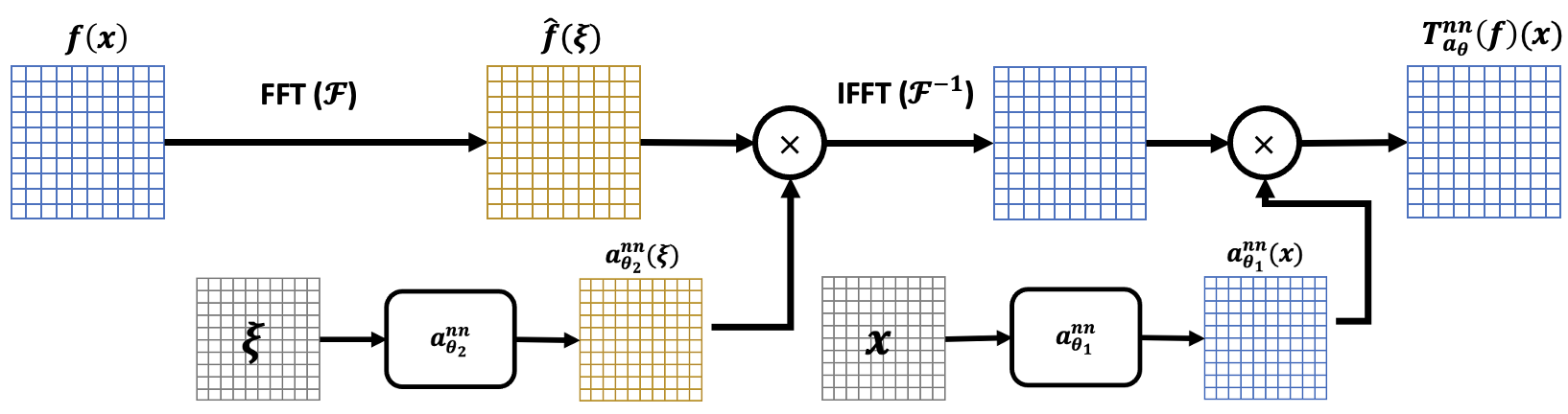
Figure 1: An architecture of a PDIO with symbol networks $a_{\theta_{1}}^{nn}(x)$ and $a_{\theta_{2}}^{nn}(\xi)$. Considering that FFT and inverse FFT are used, both the input and output are in the form of uniform mesh. Each value $a_{\theta_{1}}^{nn}(x)$ and $a_{\theta_{2}}^{nn}(\xi)$ is obtained from separate neural networks.

The primary idea in our study is to parameterize the Euclidean symbol $a(x,\xi)$ using neural networks $a^{nn}_{\theta}(x,\xi)$ to render the symbol smooth. This network is called a symbol network. The symbol network $a^{nn}_{\theta}(x,\xi)$ is assumed to be factorized into $a^{nn}_{\theta}(x,\xi)=a^{nn}_{\theta_{1}}(x)a^{nn}_{\theta_{2}}(\xi)$. Both smooth functions $a^{nn}_{\theta_{1}}(x)$ and $a^{nn}_{\theta_{2}}(\xi)$ are parameterized by fully connected neural networks. We propose a PDIO to approximate the Euclidean PDO using the symbol network and the Fourier transform as follows:

$$T_{a}(f)(x)\approx T_{a_{\theta}}^{nn}(f)(x)=a^{nn}_{\theta_{1}}(x)\mathcal{F}^{-1}\left[a^{nn}_{\theta_{2}}(\xi)\mathcal{F}[f](\xi)\right],$$ (5)

where $\mathcal{F}$ is the Fourier transform and $\mathcal{F}^{-1}$ is its inverse. The diagram of the PDIO is explained in Figure 1.

Practically, $\mathcal{F}$ and $\mathcal{F}^{-1}$ in Eq. (5) are approximated by the FFT, which is an effective algorithm that computes the discrete Fourier transform (DFT). Although the symbol network $a^{nn}_{\theta_{2}}(\xi)$ is defined on $\mathbb{R}^{n}$, the inverse DFT is evaluated only on the discrete space $\mathbb{Z}^{n}$. Therefore, the symbol network $a^{nn}_{\theta}(x,\xi)$ should be considered on the restricted domain $\mathbb{T}^{n}\times\mathbb{Z}^{n}$ (See Appendix C for details). The following section details the definitions and properties of the symbol and PDO on $\mathbb{T}^{n}\times\mathbb{Z}^{n}$. Moreover, we introduce a theorem that connects between the Euclidean symbol and the restricted Euclidean symbol.

2.3 PDOs on $\mathbb{T}^{n}\times\mathbb{Z}^{n}$

Definition 2.3.

A toroidal symbol class is a set $S^{m}_{\rho,\delta}(\mathbb{T}^{n}\times\mathbb{Z}^{n})$ consisting of the toroidal symbols $a(x,\xi)$, which are smooth in $x$ for all $\xi\in\mathbb{Z}^{n}$, and satisfy the following inequality:

$$|\bigtriangleup^{\alpha}_{\xi}\partial^{\beta}_{x}a(x,\xi)|\leq c_{\alpha\beta}\langle\xi\rangle^{m-\rho|\alpha|+\delta|\beta|},$$ (6)

for all $\alpha,\beta\in\mathbb{N}^{n}_{0}$, and for all $(x,\xi)\in\mathbb{T}^{n}\times\mathbb{Z}^{n}$. Here, $\bigtriangleup^{\alpha}_{\xi}$ are the difference operators.

The PDO corresponding to the symbol class $S^{m}_{\rho,\delta}(\mathbb{T}^{n}\times\mathbb{Z}^{n})$ can be defined as follows:

Definition 2.4.

The toroidal PDO $T_{a}:\mathcal{A}\rightarrow\mathcal{U}$ with the toroidal symbol $a(x,\xi)\in S^{m}_{\rho,\delta}(\mathbb{T}^{n}\times\mathbb{Z}^{n})$ is defined by the following equation:

$$T_{a}(f)(x)=\sum_{\xi\in\mathbb{Z}^{n}}a(x,\xi)\hat{f}(\xi)e^{2\pi i\xi x}.$$ (7)

It is well-known that the toroidal PDO $T_{a}(f)$ with $f\in C^{\infty}(\mathbb{T}^{n})$ is well defined and $T_{a}(f)\in C^{\infty}(\mathbb{T}^{n})$ [29].

Here, it is necessary to prove that the restricted symbol network $a^{nn}_{\theta}|_{\mathbb{T}^{n}\times\mathbb{Z}^{n}}$ belongs to a certain toroidal symbol class. To connect the symbol network $a^{nn}_{\theta}$ and the restricted symbol network $a^{nn}_{\theta}|_{\mathbb{T}^{n}\times\mathbb{Z}^{n}}$, we introduce a useful theorem that connects the symbols between the Euclidean symbol and the toroidal symbol.

Theorem 2.5.

[29] (Connection between two symbols) Let $0<\rho\leq 1$ and $0\leq\delta\leq 1$. A symbol $\tilde{a}\in S^{m}_{\rho,\delta}(\mathbb{T}^{n}\times\mathbb{Z}^{n})$ is a toroidal symbol if and only if there exists a Euclidean symbol $a\in S^{m}_{\rho,\delta}(\mathbb{T}^{n}\times\mathbb{R}^{n})$ such that $\tilde{a}=a|_{\mathbb{T}^{n}\times\mathbb{Z}^{n}}$.

Therefore, it is sufficient to consider if the symbol network $a^{nn}_{\theta}(x,\xi)$ belongs to a certain Euclidean symbol class.

2.4 Propositions on the symbol network and PDIO

We show that the symbol network $a^{nn}_{\theta}(x,\xi)$ with the Gaussian error linear unit (GELU) activation function is contained in a certain Euclidean symbol class using the following proposition:

Proposition 2.6.

Suppose the symbol networks $a^{nn}_{\theta_{1}}(x)$ and $a^{nn}_{\theta_{2}}(\xi)$ are fully connected neural networks with nonlinear activation GELU. Then, the symbol network $a^{nn}_{\theta}(x,\xi)=a^{nn}_{\theta_{1}}(x)a^{nn}_{\theta_{2}}(\xi)$ is in $S^{1}_{1,0}(\mathbb{T}^{n}\times\mathbb{R}^{n})$. Therefore, the restricted symbol network $\widetilde{a^{nn}_{\theta}}\overset{\mbox{{def}}}{=}a^{nn}_{\theta}|_{\mathbb{T}^{n}\times\mathbb{Z}^{n}}$ is in a toroidal symbol class $S^{1}_{1,0}(\mathbb{T}^{n}\times\mathbb{Z}^{n})$.

Remark 2.7.

Here, we focus on the most important case where $\rho=1$ and $\delta=0$, since $S^{m}_{\rho,\delta}\supset S^{m}_{1,0}$ for $0<\rho\leq 1$ and $0\leq\delta<1$ [15]. Although the proposition only considers the symbol network with GELU, it can be proved for various activation functions (See Appendix D).

Proof.

The fully connected neural network for the symbol network $a^{nn}_{\theta_{1}}(x)$ is denoted as follows:

$$Z_{1}^{[l]} =W_{1}^{[l]}A_{1}^{[l-1]}+b_{1}^{[l]}\quad(l=1,2,...,L_{1}),$$

$$A_{1}^{[l]} =\sigma(Z_{1}^{[l]})\quad(l=1,2,...,L_{1}-1),$$

where $W_{1}^{[l]}$ is a weight matrix, $b_{1}^{[l]}$ is a bias vector in the $l$-th layer of the network, $\sigma$ is an element-wise activation function, and $A_{1}^{[0]}=x$ is an input feature vector, and $Z_{1}^{[L_{1}]}=a^{nn}_{\theta_{1}}(x)$ is an output of the network with $\theta_{1}=\{W_{1}^{[l]},b_{1}^{[l]}\}_{l=1}^{L_{1}}$. Similarly, we define $W_{2}^{[l]}$, $b_{2}^{[l]}$, $Z_{2}^{[l]}$ and $A_{2}^{[l]}$ $(l=1,2,...,L_{2})$ for the neural network $a^{nn}_{\theta_{2}}(\xi)$.

The neural network $a^{nn}_{\theta_{1}}(x)$ is continuous on a compact set $\mathbb{T}^{n}$. Therefore,

$$|\partial^{\beta}_{x}a^{nn}_{\theta_{1}}(x)|\leq c_{\beta},$$ (8)

for some constant $c_{\beta}>0$ and for all $\beta\in\mathbb{N}^{n}_{0}$. For the case $|\alpha|=0$,

$$|\partial^{\alpha}_{\xi}a^{nn}_{\theta_{2}}(\xi)|=|a^{nn}_{\theta_{2}}(\xi)|=|W_{2}^{[L_{2}]}\sigma(Z_{2}^{[L_{2}-1]})+b_{2}^{[L_{2}]}|\leq c_{\alpha}\langle\xi\rangle,$$ (9)

for some constant $c_{\alpha}>0$ because the absolute value of GELU $\sigma(z)$ is bounded by linear function $|z|$. Notably,

$$\partial_{\xi}^{e_{i}}a^{nn}_{\theta_{2}}(\xi)=W_{1}^{[L_{2}]}diag\left(\sigma^{\prime}\left(Z_{1}^{[L_{2}-1]}\right)\right)\times W_{1}^{[L_{2}-1]}diag\left(\sigma^{\prime}\left(Z_{1}^{[L_{2}-2]}\right)\right)\times\cdots\times W_{1}^{[2]}diag\left(\sigma^{\prime}\left(Z_{1}^{[1]}\right)\right)W_{1}^{[1]}e_{i}.$$ (10)

This result implies that the multi-derivatives of symbol $\partial_{\xi}^{\alpha}a^{nn}_{\theta_{2}}(\xi)$ with $|\alpha|\geq 1$ consists of the product of the weight matrix and the first or higher derivatives of the activation functions. Furthermore, the derivative of GELU is bounded, and the second or higher derivatives of the function asymptotically become zero rapidly, that is, $\sigma^{(k)}\in\mathcal{S}(\mathbb{R})$ when $k\geq 2$ (see Definition D.1). Thus, we have the following inequality:

$$|\partial^{\alpha}_{\xi}a^{nn}_{\theta_{2}}(\xi)|\leq c_{\alpha}\langle\xi\rangle^{1-|\alpha|},$$ (11)

for all $\alpha\in\mathbb{N}^{n}_{0}$ with $|\alpha|\geq 1$ for some positive constants $c_{\alpha}$. Therefore, we bound the derivative of the symbol network $a^{nn}_{\theta}(x,\xi)$ as follows:

$$|\partial^{\beta}_{x}\partial^{\alpha}_{\xi}a(x,\xi)|=|\partial^{\beta}_{x}a^{nn}_{\theta_{1}}(x)||\partial^{\alpha}_{\xi}a^{nn}_{\theta_{2}}(\xi)|\leq\underbrace{c_{\alpha}c_{\beta}}_{=c_{\alpha\beta}}\langle\xi\rangle^{1-|\alpha|}.$$ (12)

Therefore, the symbol network $a^{nn}_{\theta}(x,\xi)$ is in $S^{1}_{1,0}(\mathbb{T}^{n}\times\mathbb{R}^{n})$ as defined in Definition 2.1. Finally, using Theorem 2.5, we deduce that $\widetilde{a^{nn}}=a^{nn}|_{\mathbb{T}^{n}\times\mathbb{Z}^{n}}$ is in $S^{1}_{1,0}(\mathbb{T}^{n}\times\mathbb{Z}^{n})$. ∎

We introduce the theorem on the boundedness of a toroidal PDO as follows:

Theorem 2.8.

[29] (Boundedness of a toroidal PDO in the Sobolev space) Let $m\in\mathbb{R}$ and $k\in\mathbb{N}$, which is the smallest integer greater than $\frac{n}{2}$, and let $a:\mathbb{T}^{n}\times\mathbb{Z}^{n}\rightarrow\mathbb{C}$ such that

$$|\partial_{x}^{\beta}\bigtriangleup_{\xi}^{\alpha}a(x,\xi)|\leq C\langle\xi\rangle^{m-|\alpha|}\quad\text{for all }(x,\xi)\in\mathbb{T}^{n}\times\mathbb{Z}^{n},$$ (13)

and all multi-indices $\alpha$ such that $|\alpha|\leq k$ and all multi-indices $\beta$. Then the corresponding toroidal PDO $T_{a}$ defined in Definition 2.4 extends to a bounded linear operator from the Sobolev space $W^{p,s}(\mathbb{T}^{n})$ to the Sobolev space $W^{p,s-m}(\mathbb{T}^{n})$ for all $1<p<\infty$ and any $s\in\mathbb{R}$.

The restricted symbol network $\widetilde{a^{nn}_{\theta}}$ is in a toroidal symbol class $S^{1}_{1,0}(\mathbb{T}^{n}\times\mathbb{Z}^{n})$ from Proposition 2.6. Thus, it satisfies the condition in Theorem 2.8. Thus, the PDIO $T_{a_{\theta}}^{nn}$ with the restricted symbol network $\widetilde{a^{nn}_{\theta}}$ is a bounded linear operator from $W^{p,s}(\mathbb{T}^{n})$ to $W^{p,s-1}(\mathbb{T}^{n})$ for all $1<p<\infty$ and $s\in\mathbb{R}$. This implies that the PDIO is a continuous operator between the Sobolev spaces. Therefore, we expect that the PDIO can be applied to a neural operator (17) to obtain a smooth and general solution operator. A description of its application to neural operator is explained in Section 3.

2.5 Time dependent PDIO

Consider the time-dependent PDE

$$\frac{\partial u}{\partial t}=\mathcal{L}u,\quad u(x,0)=u_{0}(x),\quad(x,t)\in\mathbb{T}^{n}\times[0,\infty).$$ (14)

This is well-posed and has the unique solution provided that the operator $\mathcal{L}$ is semi-bounded [11]. The solution is given by $u(x,t)=e^{t\mathcal{L}}u_{0}(x)$. In the case of the 1D heat equation, $\mathcal{L}$ is $c\partial_{xx}$ with diffusivity constant $c$. Then, the solution of the heat equation is given by

$$u(x,t)=\sum_{\xi\in\mathbb{Z}}e^{-4\pi^{2}\xi^{2}ct}\hat{u}_{0}(\xi)e^{2\pi ix\xi}.$$ (15)

This shows that the mapping from $u_{0}(x)$ to $u(x,t)$ is the PDO with the symbol $e^{-4\pi^{2}\xi^{2}ct}$. Consequently, we propose the time dependent PDIOs given as follows:

$$T_{a}(f)(x,t)\approx T_{a_{\theta}}^{nn}(f)(x,t)=a^{nn}_{\theta_{1}}(x,t)\mathcal{F}^{-1}\left[a^{nn}_{\theta_{2}}(\xi,t)\mathcal{F}[f](\xi)\right],$$ (16)

where $a_{\theta_{1}}^{nn}(x,t)$ and $a_{\theta_{2}}^{nn}(\xi,t)$ are time dependent symbol networks. In the experiment, we verify that the time dependent PDIOs approximate time dependent symbol accurately even in a finer time grid than a time grid used for training. Therefore, we can obtain the continuous-in-time solution operator of the PDEs.

3 Application to a nonlinear operator combined with a neural operator

In many problems, the solution operator of the PDE is nonlinear. Although the PDIO by itself is a linear operator, it can be combined with a nonlinear architecture to learn highly nonlinear operators. We introduce a neural operator architecture to learn infinite-dimensional operators effectively.

3.1 Neural operator [23]

Inspired by Green’s functions of elliptic PDEs, [23] proposed an iterative neural operator to approximate the solution operators of parametric PDEs. To find a map from the function $f(x)$ to the solution $u(x)$, the input $f(x)$ is lifted to a higher representation $f_{0}(x)=P(f(x))$. Next, the iterations $f_{0}\mapsto f_{1}....\mapsto f_{T}$ are applied using the update $f_{t}\mapsto f_{t+1}$ formulated using the following expression:

$$f_{t+1}(x)=\sigma\left(Wf_{t}(x)+\mathcal{K}_{\phi}(f_{t})(x)\right),$$ (17)

for $t=0,...,T-1$, where $W$ is a local linear transformation, $\mathcal{K}_{\phi}$ is an integral operator $\mathcal{K}$ parameterized by $\phi$, and $\sigma$ is a nonlinear activation function. The output $u(x)=Q(f_{T}(x))$ is the projection of $f_{T}(x)$ by the local transformation $Q$. The integral operator $\mathcal{K}_{\phi}$ is parameterized using the message passing on graph networks. Furthermore, [21] proposed a Fourier integral operator in which the integral operator $\mathcal{K}_{\phi}$ is a convolution operator.

3.2 Proposed PDNO

Table 1: Benchmark (relative $L^{2}$ error) on Burgers’ equation on different resolution $s$.

Networks	$s=256$	$s=512$	$s=1024$	$s=2048$	$s=4096$	$s=8192$
PDNO ($a(x,\xi)$)	0.000685	0.000849	0.00110	0.00118	0.00178	0.00165
PDNO ($a(\xi)$)	0.000903	0.00122	0.00125	0.00129	0.00191	0.00225
MWT Leg	0.00199	0.00185	0.00184	0.00186	0.00185	0.00178
MWT Chb	0.00402	0.00381	0.00336	0.00395	0.00299	0.00289
FNO	0.00332	0.00333	0.00377	0.00346	0.00324	0.00336

A structure consisting of the PDIO is introduced for $\mathcal{K}_{\phi}$ in Eq. (17). The proposed structure is similar to a fully connected neural network structure. Precisely, let $f_{t}(x)\in\mathbb{R}^{c_{in}}$, where $f_{t}(x)=[f_{t,i}(x):\mathbb{R}^{n}\rightarrow\mathbb{R}]_{i=1}^{c_{in}}$ with the number of input channels $c_{in}$ and $x\in\mathbb{R}^{n}$. Then, the integral operator $\mathcal{K}_{a}$ is expressed as follows:

$$\mathcal{K}_{a}(f_{t})(x)\overset{\mbox{{def}}}{=}\left[\sum_{i=1}^{c_{in}}T_{a_{\theta}}^{nn}(f_{t})(x)\right]_{j=1}^{c_{out}}=\left[\sum_{i=1}^{c_{in}}a_{\theta_{1},i,j}^{nn}(x)\mathcal{F}^{-1}\left[a_{\theta_{2},i,j}^{nn}(\xi)\mathcal{F}[f_{t,i}](\xi)\right](x)\right]_{j=1}^{c_{out}},$$ (18)

where $\theta_{1},\theta_{2}$ are the parameters of each symbol network and the $c_{out}$ is the number of output channels with $f_{t+1}(x)\in\mathbb{R}^{c_{out}}$. Indeed, the proposed integral operator (Eq. (18)) is a linear combination of PDIOs (Eq. (5)), as displayed in Figure 2. Therefore, the solution operator can be approximated by a model combining the proposed integral operator with the neural operator (Eq. (17)). The combined model is called a pseudo-differential neural operator (PDNO). In the experiments, we use three separate symbol networks $a_{\theta_{1}}^{nn}(x)$, $\text{Re}\left(a_{\theta_{2}}^{nn}(\xi)\right)$, and $\text{Im}\left(a_{\theta_{2}}^{nn}(\xi)\right)$. Each symbol network has input dimension $x,\xi\in\mathbb{R}^{n}$ and output dimension $c_{in}\times c_{out}$.

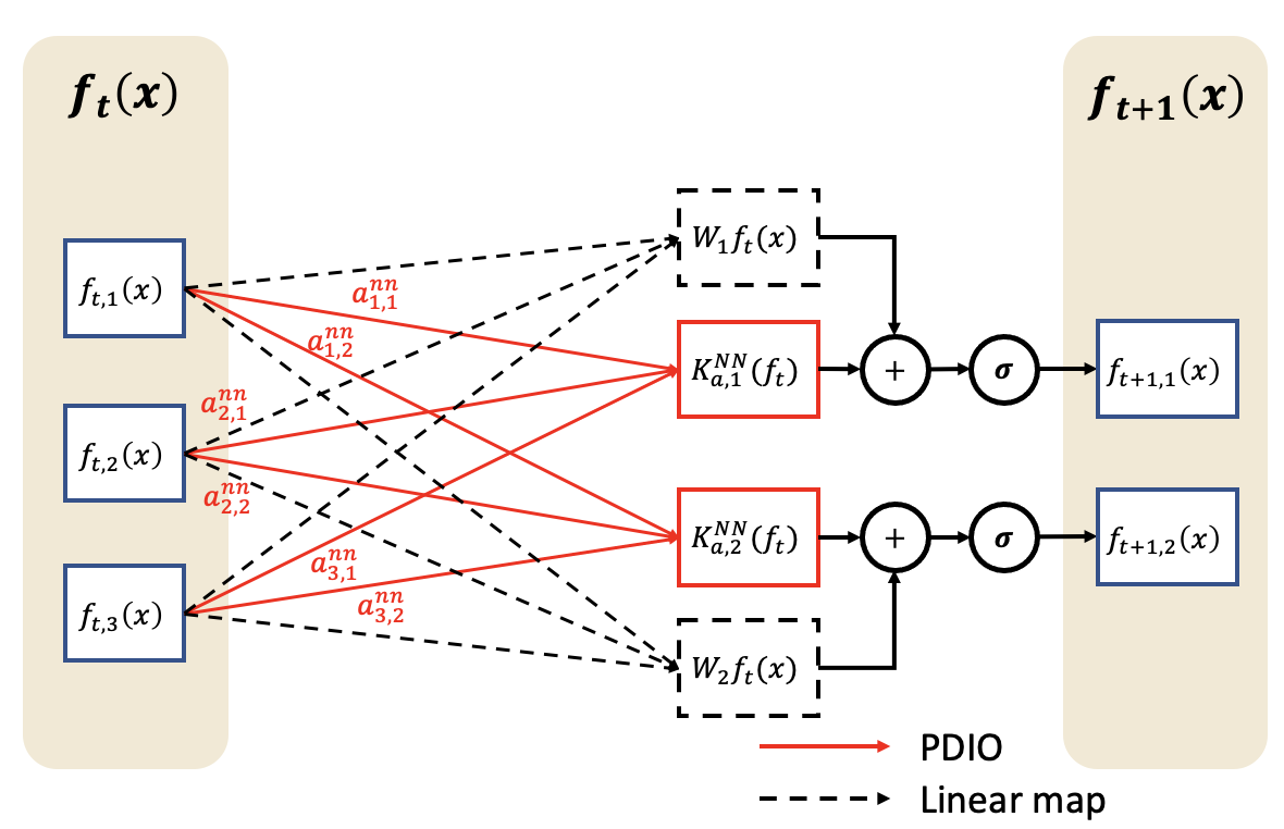
Figure 2: Structure of Eq. (17) using the integral operator $\mathcal{K}_{a}$ in Eq. (18) with $c_{in}=3$ and $c_{out}=2$. Each black solid line represents a PDIO with symbol network $a_{ij}^{nn}$.

3.3 Comparing with Fourier integral operator

In the Fourier neural operator proposed in [21], a neural operator structure with the integral operator $\mathcal{K}_{R}$ called Fourier integral operator was introduced, which can be expressed as follows:

$$\mathcal{K}_{R}[f_{t}](x)=\left[\mathcal{F}^{-1}\left[\sum_{i=1}^{c_{in}}R_{ij}(\xi)\cdot\mathcal{F}[f_{t,j}](\xi)\right](x)\right]_{j=1}^{c_{out}}.$$ (19)

As $\mathcal{F}^{-1}$ is a linear transformation, the summation and $\mathcal{F}^{-1}$ is commutative in Eq. (19). Thus, we can rewrite

$$\mathcal{K}_{R}[f_{t}](x)=\left[\sum_{j=1}^{c_{in}}\mathcal{F}^{-1}\left[R_{ij}(\xi)\cdot\mathcal{F}[f_{t,j}](\xi)\right](x)\right]_{j=1}^{c_{out}}.$$ (20)

Therefore, each output channel of $\mathcal{K}_{R}$ is also interpreted as a linear combination of PDOs with the parametric symbol $R_{ij}(\xi)$. Note that the parameter $R_{ij}(\xi)$ is directly parameterized on the discrete space $\mathbb{Z}^{n}$. The parameters $R_{ij}(\xi)$ may not satisfy the condition of the toroidal symbol (Eq. (6)) in Definition 2.3. Furthermore, parameters $R_{ij}(\xi)$ only consider the dependency on $\xi$, while the symbol network $a^{nn}_{\theta}(x,\xi)$ has a dependency on $x$. Therefore, we expect the proposed model using the symbol network, which belongs to a certain symbol class, to exhibit enhanced performance.

4 Experiments

4.1 Toy example : 1D heat equation

In this experiment, we verify whether the proposed time-dependent PDIO actually learns the symbol of the analytic PDO. We consider the 1D heat equation given in Eq. (14). The solution operator of the 1D heat equation is a PDO, which is given in Eq. (15). We aim to learn the mapping from the initial state and time $(u_{0}(x),t)$ to the solution $u(x,t)$. The initial state $u_{0}(x)$ is generated from the Gaussian random field $\mathcal{N}(0,7^{4}(-\Delta+7^{2})^{-2.5})$ with the periodic boundary conditions. $\Delta$ denotes the Laplacian. The diffusivity constant $c$ and the spatial resolution are set to 0.05 and $2^{10}=1024$, respectively. We use 1000 pairs of train data comprising 10 time grids $t=0.05+0.1n$ ($n=0,1,...,9$) for each of the 100 initial states. We test for 20 initial states at finer time grids $t=0.05+0.05n$ ($n=0,1,...,19$). The time dependent PDIO (Eq. (16)) is used and achieves a relative $L^{2}$ error lower than 0.01 on both the traning and test sets. Figure 3 shows the symbol network and the analytic symbol given in Eq. (15) on $(\xi,t)\in[-12,12]\times[0.05,1]$. Although the PDIO learns from a sparse time grid, it obtains an accurate symbol for all $t\in[0.05,1]$.

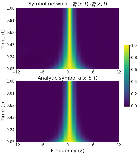
Figure 3: Visualization of the learned symbol from the time dependent PDIO $a_{\theta_{1}}^{nn}(x,t)a_{\theta_{2}}^{nn}(\xi,t)$ (top) and analytic symbol $a(x,\xi,t)=e^{-4\times 0.05\pi^{2}\xi^{2}t}$ (bottom) of the solution operator of the 1D heat equation. Note that learned $a_{\theta_{1}}^{nn}(x,t)$ is a constant function according to $x$. i.e. $a_{\theta_{1}}^{nn}(x,t)=c(t)$ (See Figure 7). Therefore, it does not require an $x$-coordinate to plot the learned symbol.

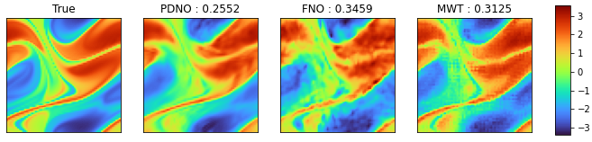
Figure 4: Example of a prediction on the Navier-Stokes data with $\nu$=1e-5 showing the prediction $w(x,19)$ from inputs $[w(x,0),...,w(x,9)]$. Each value on the top of the figure is the relative $L^{2}$ error between the true $w(x,19)$ and each prediction.

.

4.2 Nonlinear solution operators of PDEs

In this section, we verify the PDNO on a nonlinear PDEs dataset. For all the experiments, we use the PDNO that consists of four iterations of the network described in Figure 2 and Eq. (18) with a nonlinear activation GELU. Fully connected neural networks are used for symbol networks up to layer three and hidden dimension 64. The relative $L^{2}$ error is used for the loss function. Detailed hyperparameters are contained in Appendix B. We do not truncate the Fourier coefficient in any of the layers, indicating that we use all of the available frequencies from $-[\frac{s}{2}]$ to $\lceil\frac{s}{2}\rceil-1$. This is because PDNO does not require additional learning parameters, even if all frequencies are used. However, because evaluations are required at numerous grid points, considerable memory is required in the learning process. In practical settings, it is recommended to truncate the frequency space into appropriate maximum modes $k_{max}$. We observed that there was little degradation in performance even if truncation was used (See Appendix E.2). All experiments were conducted using up to five NVIDIA A5000 GPUs with 24 GB memory.

Benchmark models

We compare the proposed model with the multiwavelet-based model (MWT) and the Fourier neural operator (FNO), which are the state-of-the-art approaches based on the neural operator architecture. For the difference between PDNO ($a(x,\xi)$) and PDNO ($a(\xi)$), see Section 4.3. We conducted the experiments on three PDEs, namely Burgers’ equation, Darcy flow, and the Navier-Stokes equation. In the case of Burgers’ equation and the Navier-Stokes equation, we use the same data attached in [21]. In the case of Darcy flow, we regenerate the data according to the same data generation scheme.

Burgers’ equation

The 1D Burgers’ equation is a nonlinear PDE, which describes the interaction between the effects of nonlinear convection and diffusion as follows:

$$\begin{cases}\frac{\partial u}{\partial t}=-u\cdot\frac{\partial u}{\partial x}+\nu\frac{\partial^{2}u}{\partial x^{2}},&(x,t)\in(0,1)\times(0,1],\\ u(x,0)=u_{0}(x),&x\in(0,1),\end{cases}$$ (21)

where $u_{0}$ is the initial state and $\nu$ is the viscosity. We aim to learn the nonlinear mapping from the initial state $u_{0}(x)$ to the solution $u(x,1)$ at $t=1$. We use the same Burgers’ data used in [21]. The initial state $u_{0}(x)$ is generated from the Gaussian random field $\mathcal{N}(0,5^{4}(-\Delta+25I)^{-2})$ with the periodic boundary conditions. The viscosity $\nu$ and the finest spatial resolution are set to 0.1 and $2^{13}=8192$, respectively. The lower resolution dataset is obtained by subsampling. We experiment with the same hyperparameters for all resolutions. We use 1000 train pairs and 100 test pairs.

The results from the Burgers data are listed in Table 1 along with the different resolutions $s$. The proposed model outperforms both MWT and FNO for all resolutions. Remarkable improvements are obtained especially in the case of low resolutions.

Darcy flow

The Darcy flow problem is a diffusion equation with an external force, which describes the flow of a fluid through a porous medium. The steady state of the Darcy flow on the unit box is expressed as follows:

$$\begin{cases}\nabla\cdot(a(x)\nabla u(x))=f(x),&x\in(0,1)^{2},\\ u(x)=0,&x\in\partial(0,1)^{2},\end{cases}$$ (22)

where $u$ is density of the fluid, $a(x)$ is the diffusion coefficient, and $f(x)$ is the external force. We aim to learn the nonlinear mapping from $a(x)$ to the steady state $u(x)$, fixing the external force $f(x)=1$. The diffusion coefficient $a(x)$ is generated from $\psi_{\#}\mathcal{N}(0,(-\Delta+9I)^{-2})$, where $\Delta$ is the Laplacian with zero Neumann boundary conditions, and $\psi_{\#}$ is the pointwise push forward, defined by $\psi(x)=12$ if $x>0$, 3 elsewhere. The coefficient imposes the ellipticity on the differential operator $\nabla\cdot(a(x)\nabla)(\cdot)$. We generate $a(x)$ and $u(x)$ using the second order FDM on a $512\times 512$ grid. The lower resolution dataset is obtained by subsampling. We use 1000 train pairs and 100 test pairs and fixed the hyperparameters for all resolutions.

The results on the Darcy flow are presented in Table 2 for various resolutions $s$. The proposed model achieves the lowest relative error for all resolutions. In the case of $s=32$, particularly, MWT and FNO exhibit the highest errors. Furthermore, the proposed model maintains its performance even at low resolutions.

Table 2: Benchmark (relative $L^{2}$ error) on Darcy Flow for different resolutions $s$.

Networks	$s=32$	$s=64$	$s=128$	$s=256$	$s=512$
PDNO ($a(x,\xi)$)	0.0033	0.0025	0.0016	0.0014	0.0019
PDNO ($a(\xi)$)	0.0038	0.0028	0.0025	0.0025	0.0022
MWT Leg	0.0162	0.0108	0.0093	0.0088	0.0092
FNO	0.0178	0.0112	0.0103	0.0101	0.0102

Navier-Stokes equation

Navier-Stokes equation describes the dynamics of a viscous fluid. In the vorticity formulation, the incompressible Navier-Stokes equation on the unit torus can be expressed as follows:

$$\begin{cases}\frac{\partial w}{\partial t}+u\cdot\nabla w-\nu\Delta w=f,&(x,t)\in(0,1)^{2}\times(0,T],\\ \nabla\cdot u=0,&(x,t)\in(0,1)^{2}\times[0,T],\\ w(x,0)=w_{0}(x),&x\in(0,1)^{2},\end{cases}$$ (23)

where $w$ is the vorticity, $u$ is the velocity field, $\nu$ is the viscosity, and $f$ is the external force. We use the same Navier-Stokes data used in [21] to learn the nonlinear mapping from $w(x,0),....,w(x,9)$ to $w(x,10),...,w(x,T)$, fixing the force $f(x)=0.1(\sin(2\pi(x_{1}+x_{2}))+\cos(2\pi(x_{1}+x_{2})))$. The initial condition $w_{0}(x)$ is sampled from $\mathcal{N}(0,7^{1.5}(-\Delta+7^{2}I)^{-2.5})$ with periodic boundary conditions. We experiment with four Navier-Stokes datasets:$(\nu,T,N)=(10^{-3},50,1000),(10^{-4},30,1000),(10^{-4},30,10000)$, and $(10^{-5},20,1000)$, where $\nu$ is the viscosity, $T$ is the final time to predict, and $N$ is the number of training samples. Notably, the lower the viscosity, the more difficult the prediction. All datasets comprise $64\times 64$ resolutions.

We employ a recurrent architecture to propagate along the time domain. From $w(x,0),....,w(x,9)$, the model predicts the vorticity at $t=10$, $\bar{w}(x,10)$. Then, from $w(x,1),...,w(x,9),\bar{w}(x,10)$, the model predicts the next vorticity $\bar{w}(x,11)$. We repeat this process until $t=T$.

For each experiment, we use 200 test samples. In the case of $(\nu,T,N)=(10^{-3},50,1000)$, we use a batch size 10 or 20 otherwise. Furthermore, we use fixed hyperparameters for the four experiments.

The results on the Navier-Stokes equation are presented in Table 3. In all four datasets, the proposed model exhibits comparable or superior performances. Notably, the relative error improves considerably for $(\nu,T,N)=(10^{-5},20,1000)$, exhibiting the lowest viscosity. Figure 4 displays a sample prediction at $t=19$, which is highly unpredictable.

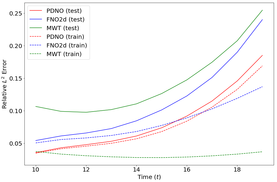
Figure 5: Comparison of the train and the test relative $L^{2}$ error by time horizon $t=10,...,19$ on the Navier-Stokes equation with $\nu=1e-5$.

Table 3: Benchmark (relative $L^{2}$ error) on the Navier-Stokes equation on the various viscosity $\nu$, the time horizon $T$, and the number of data $N$.

	$\nu=1e-3$	$\nu=1e-4$	$\nu=1e-4$	$\nu=1e-5$
Networks	$T=50$	$T=30$	$T=30$	$T=20$
	$N=1000$	$N=1000$	$N=10000$	$N=1000$
PDNO	0.00903	0.1320	0.0679	0.1093
MWT Leg	0.00625	0.1518	0.0667	0.1541
MWT Chb	0.00720	0.1574	0.0720	0.1667
FNO-2D	0.0128	0.1559	0.0973	0.1556
FNO-3D	0.0086	0.1918	0.0820	0.1893

4.3 Additional experiments

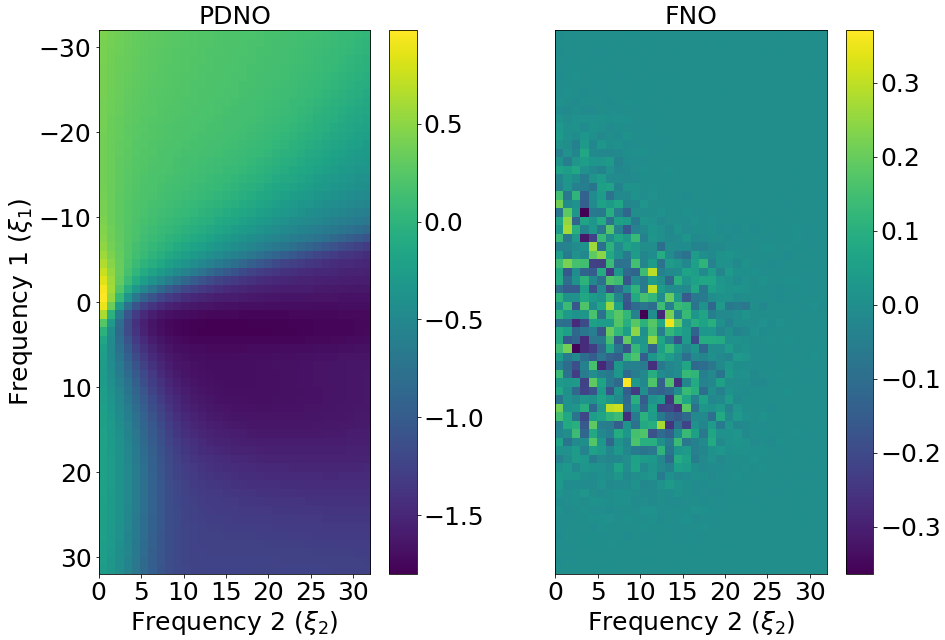
Figure 6: Examples of the real part of learned symbol $a_{ij}^{nn}(\xi)$ from the Navier-Stokes data with $\nu=1e-5$. $x$-axis and $y$-axis represent frequency domains. As we used real valued functions, the second coordinate is half the first.

On Burgers’ equation and Darcy flow, we perform an additional experiment, which does not use a symbol network $a_{\theta_{1}}^{nn}(x)$, but only use $a_{\theta_{2}}^{nn}(\xi)$. In this case, the PDNO has the same structure as FNO except that the symbol is smooth. See PDNO ($a(\xi)$) in Table 1 and Table 2. Although less than the original PDNO, the results of the PDNO without the dependency of the $x$-symbol perform better than the other models, including FNO. This shows why the smoothness of the symbol of PDNO is important.

On the Navier-Stokes equation with $\nu=1e-5$, we compare the train and the test relative $L^{2}$ errors along time $t$ in Figure 5. All models show that the test errors grow exponentially according to time $t$. Among them, PDNO consistently demonstrates the least test errors for all time $t$. More notable is the difference between the solid lines and the dashed lines, showing that MWT and FNO suffer from overfitting, whereas PDNO does not. This might be related to the smoothness of the symbols of models. Furthermore, the symbols of PDNO and the FNO are visualized in Figure 6.

5 Conclusion

Based on the theory of PDO, we developed a novel PDIO and PDNO framework that efficiently learns mappings between functions spaces. The proposed symbol networks are in a toroidal symbol class that renders the corresponding PDIOs continuous between Sobolev spaces on the torus, which can considerably improve the learning of the solution operators in most experiments. This study revealed an excellent ability for learning operators based on the theory of PDO. However, there is room for improvement in highly complex PDEs such as the Navier Stokes equation, and the time dependent PDIOs are difficult to apply to nonlinear architecture. We expect to solve these problems by using advanced operator theories [5, 13, 6], and the operator learning will solve engineering and physical problems.

Appendix A Notations

We list the main notations throughout this paper in Table 4.

Table 4: Notations

Notations	Descriptions
$\mathcal{A}$	an input function space
$\mathcal{U}$	an output function space
$T:\mathcal{A}\rightarrow\mathcal{U}$	an operator from $\mathcal{A}$ to $\mathcal{U}$
$x\in\mathbb{R}^{n}\text{ or }\mathbb{T}^{n}$	a variable in the spatial domain
$\xi\in\mathbb{R}^{n}\text{ or }\mathbb{Z}^{n}$	a variable in the Fourier space
$\hat{f}(\xi)$	Fourier transform of function $f(x)$
$S^{m}_{\rho,\delta}$	an Euclidean (or toroidal) symbol class
$a(x,\xi)\in S^{m}_{\rho,\delta}$	an Euclidean (or toroidal) symbol
$a^{nn}_{\theta}(x,\xi)$	a symbol network parameterized by $\theta$
$T_{a}:\mathcal{A}\rightarrow\mathcal{U}$	a PDO with the symbol $a(x,\xi)$
$T^{nn}_{a_{\theta}}:\mathcal{A}\rightarrow\mathcal{U}$	a PDIO with a symbol network $a_{\theta}(x,\xi)$
$\mathcal{F}:\mathcal{A}\rightarrow\mathcal{U},\mathcal{F}^{-1}:\mathcal{U}\rightarrow\mathcal{A}$	Fourier transform and its inverse
$\|\xi\|$	Euclidean norm
$\langle\xi\rangle$	$(1+\|\xi\|^{2})^{\frac{1}{2}}$
$\bigtriangleup_{\xi}^{\alpha}$	a difference operator of order $\alpha$ on $\xi$
$k_{max}$	the maximum number of Fourier modes

Appendix B Hyperparameters

Table 5: Hyperparameters for learning PDNOs on each dataset. # layers, # hidden and activation are for symbol networks.

Data	batch size	learning rate	weight decay	epochs	step size	# channel	# layers	# hidden	activation
Heat equation	20	$1\times 10^{-2}$	$1\times 10^{-6}$	10000	2000	1	2	40	GELU
Burgers’ equation	20	$5\times 10^{-3}$	0	1000	100	64	2	64	TANH
Darcy flow	20	$1\times 10^{-2}$	$1\times 10^{-6}$	1000	200	20	3	32	GELU
Navier-Stokes equation	20	$5\times 10^{-3}$	$1\times 10^{-6}$	1000	200	20	2	32	GELU

Appendix C The reason for considering the symbol network on domain $\mathbb{T}^{n}\times\mathbb{Z}^{n}$

In this section, we detail why the proposed model should be addressed in $\mathbb{T}^{n}\times\mathbb{Z}^{n}$ instead of $\mathbb{T}^{n}\times\mathbb{R}^{n}$. For convenience, we assume that $n=1$. Let $f:\mathbb{T}\rightarrow\mathbb{R}$ and its $N$ points discretization $f(\frac{1}{N})=y_{0}$, $f(\frac{2}{N})=y_{1}$, … $f(\frac{N}{N})=y(1)=y_{N-1}$. Then, the discrete Fourier transform (DFT) of the sequence $\{y_{n}\}_{0\leq n\leq N-1}$ is expressed by the following:

$$\xi_{k}=\frac{1}{N}\sum_{n=0}^{N-1}y_{n}e^{-2\pi ik\frac{n}{N}}$$ (24)

and the inverse discrete Fourier transform (IDFT) of $\{\xi_{k}\}_{0\leq k\leq N-1}$ is expressed as follows:

$$y_{n}=\sum_{k=0}^{N-1}\xi_{k}e^{2\pi ik\frac{n}{N}}.$$ (25)

As $N$ goes $\infty$, we can see that

$$\lim_{N\rightarrow\infty}\xi_{k}=\lim_{N\rightarrow\infty}\frac{1}{N}\sum_{n=0}^{N-1}f(\frac{n+1}{N})e^{-2\pi ik\frac{n}{N}}\rightarrow\int_{0}^{1}f(x)e^{-2\pi ikx}\,dx=\hat{f}(k)$$ (26)

and

$$\lim_{N\rightarrow\infty}y_{n}=\lim_{N\rightarrow\infty}f(\underbrace{\frac{n}{N}}_{x}+\frac{1}{N})=\lim_{N\rightarrow\infty}\sum_{k=0}^{N-1}\xi_{k}e^{2\pi ik\frac{n}{N}}\rightarrow\sum_{k=0}^{\infty}\hat{f}(k)e^{2\pi ikx}=f(x),$$ (27)

where $x=\frac{n}{N}$. Thus, DFT is an approximation of integral on $\mathbb{T}$ and IDFT is an approximation of infinity sum on $\mathbb{Z}$. Therefore, the theory of PDO on $\mathbb{T}^{n}\times\mathbb{Z}^{n}$ is more suited to our model.

Appendix D Activation functions for symbol network

In this section, we discuss the activation function for the symbol network. We proved the Proposition 2.6 when GELU activation function is used for the symbol network. Not only GELU, but also other activation functions can be used for the symbol network. To explain this, we first define the Schwartz space [28] as follows:

Definition D.1.

The Schwartz space $\mathcal{S}(\mathbb{R}^{n})$ is the topological vector space of functions $f:\mathbb{R}^{n}\rightarrow\mathbb{C}$ such that $f\in C^{\infty}(\mathbb{R}^{n})$ and

$$z^{\alpha}\partial^{\beta}f(z)\rightarrow 0,\quad\text{as }|z|\rightarrow\infty,$$ (28)

for every pair of multi-indices $\alpha,\beta\in\mathbb{N}^{n}_{0}$.

That is, the Schwartz space consists of smooth functions whose derivatives decay at infinity faster than any power. As mentioned in the proof of Proposition 2.6, it can be easily shown that the second or higher derivatives of GELU is in the Schwartz space $\mathcal{S}(\mathbb{R})$. Because GELU is defined as $\sigma(z)=z\Phi(z)$ with $\Phi(z)=\frac{1}{\sqrt{2\pi}}\int_{-\infty}^{z}\exp(-u^{2}/2)du$, the second or higher derivatives of GELU is the sum of exponential decay functions $\exp(-z^{2}/2)$. Thus, the second or higher derivatives of the function is in the Schwartz space, that is, $\sigma^{(k)}\in\mathcal{S}(\mathbb{R})$ when $k\geq 2$.

Next, we prove that another activation function $\phi(z)$ is in symbol class $S^{1}_{1,0}(\mathbb{T}^{n}\times\mathbb{R}^{n})$ if the difference between the function $\phi(z)$ and GELU $\sigma(z)$ is in the Schwartz space. We call a function like $\phi(z)$ a GELU-like activation function. It can be easily shown that the function $\phi(z)$ is bounded by linear function $|z|$ because GELU is bounded by the linear function. Because the Schwartz space is closed under differentiation, $\phi(z)-\sigma(z)\in\mathcal{S}(\mathbb{R})$ implies $\phi^{(k)}(z)-\sigma^{(k)}(z)\in\mathcal{S}(\mathbb{R})$ for $k\in\mathbb{N}$. Because GELU satisfies $\sigma^{\prime}(z)\leq c_{\alpha}$ and $\sigma^{(k)}\in\mathcal{S}(\mathbb{R})$ when $k\geq 2$, the activation function $\phi(z)$ also satisfies $\phi^{\prime}(z)\leq c_{\alpha}$ and $\phi^{(k)}\in\mathcal{S}(\mathbb{R})$ when $k\geq 2$. Therefore, the proof of Proposition 2.6 can be obtained by changing another activation function $\phi(z)$ instead of GELU $\sigma(z)$. GELU-like activation functions, such as the Softplus [8], and Swish [27] etc., satisfy the aforementioned assumption so that it can be used for the symbol network in our PDIO.

We can easily show that the symbol network $a^{nn}_{\theta}(x,\xi)$ with $\tanh(z)=\frac{e^{z}-e^{-z}}{e^{z}+e^{-z}}$ is in $S^{0}_{1,0}(\mathbb{T}^{n}\times\mathbb{R}^{n})$. In the proof of Proposition 2.6, we used the characteristic of GELU and its high derivatives. Tanh function is bounded and the first or higher derivatives of tanh function is in the Schwartz space. Therefore, neural network $a^{nn}_{\theta_{2}}(\xi)$ satisfies the following boundedness:

$$|\partial^{\alpha}_{\xi}a^{nn}_{\theta_{2}}(\xi)| \leq c_{\alpha},\quad\text{if }|\alpha|=0,$$ (29)

$$|\partial^{\alpha}_{\xi}a^{nn}_{\theta_{2}}(\xi)| \leq c_{\alpha}\langle\xi\rangle^{-|\alpha|},\quad\text{if }|\alpha|\geq 1.$$ (30)

Note that the boundedness of the neural network $a^{nn}_{\theta_{1}}(x)$ is same in the case of GELU. Thus, we can bound the derivative of the symbol network $a^{nn}_{\theta}(x,\xi)$ as follows:

$$|\partial^{\beta}_{x}\partial^{\alpha}_{\xi}a(x,\xi)|\leq c_{\alpha\beta}\langle\xi\rangle^{-|\alpha|}.$$ (31)

Therefore, the symbol network with tanh activation function is in $S^{0}_{1,0}(\mathbb{T}^{n}\times\mathbb{R}^{n})$. Similarly, it is easy to prove that sigmoid function $\frac{1}{1+e^{-z}}$ also is in a symbol class $S^{0}_{1,0}(\mathbb{T}^{n}\times\mathbb{R}^{n})$. Therefore, the PDIOs with these two activation functions are bounded linear operators from the Sobolev space $W^{p,s}(\mathbb{T}^{n})$ to the Sobolev space $W^{p,s}(\mathbb{T}^{n})$ for all $1<p<\infty$ and any $s\in\mathbb{R}$.

Appendix E Additional figures and experiments

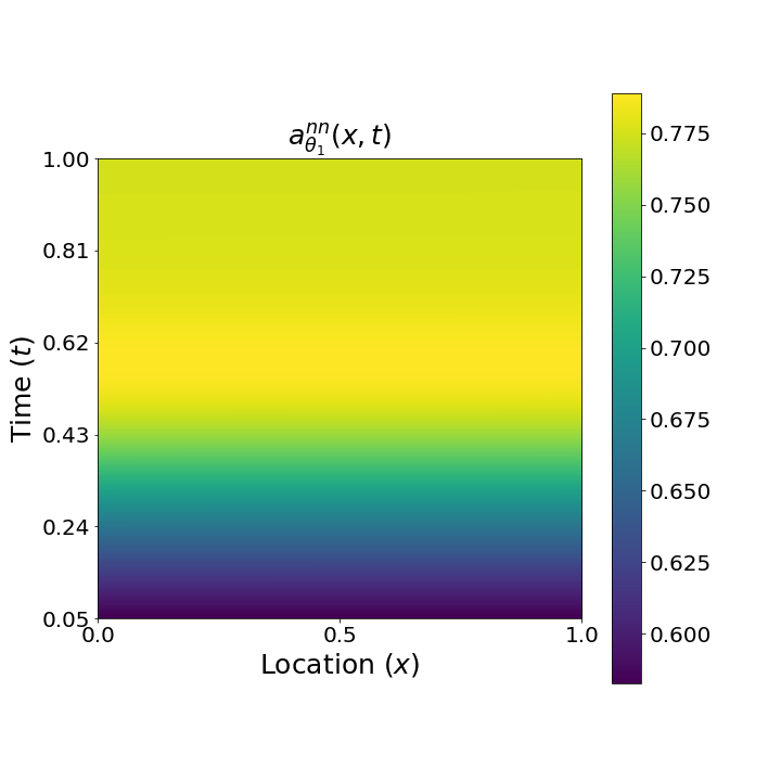
Figure 7: Learned symbol $a_{\theta_{1}}^{nn}(x,t)$ from 1D heat equation.

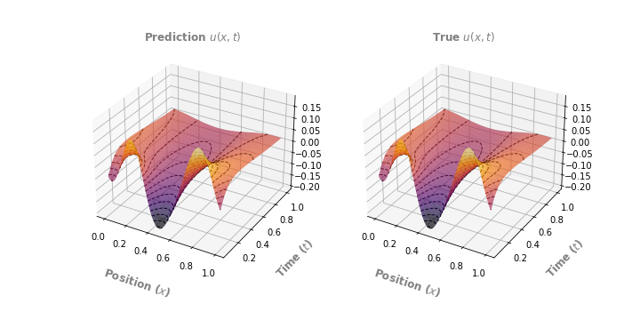
Figure 8: A sample of prediction on 1D heat equation from a PDIO. The model is trained on $1024\times 10$ dataset and evaluated on $1024\times 20$. Dashed lines on the surface are contour lines.

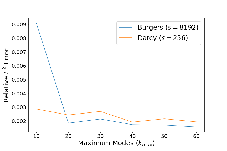
Figure 9: Test relative $L^{2}$ error that depends on maximum modes $k_{max}$ of PDNO on Burgers’ equation (resolution $s=8192$) and Darcy flow (resolution $s=256$).

E.1 1D heat equation : Symbol network $a_{\theta_{1}}^{nn}(x,t)$.

In 1D heat equation experiments, we assume that the symbol is decomposed by $a(x,\xi,t)\approx a_{\theta_{1}}^{nn}(x,t)\times a_{\theta_{2}}^{nn}(\xi,t)$. In Figure 7, it shows the learned symbol network $a_{\theta_{1}}^{nn}(x,t)$ on $(x,t)\in\mathbb{T}\times[0.05,1]$. We can see that $a_{\theta_{1}}^{nn}(\cdot,t)$ is almost a constant function for each $t\in[0.05,1]$. In this respect, $a_{\theta_{1}}^{nn}(x,t)$ is treated as a function of $t$ by taking the average along $x$-dimension to visualize $a_{\theta_{1}}^{nn}(x,t)a_{\theta_{2}}^{nn}(\xi,t)$ in Figure 3.

In addition, Figure 8 visualizes a sample prediction on 1D heat equation.

E.2 Changes in errors according to $k_{max}$.

As mentioned in Section 4.2, we use all possible modes. Although PDNO does not require additional parameters to use all modes, it demands more memory in the learning process. So, we perform an additional experiments on Burgers equation and Darcy flow by limiting the number of modes $k_{max}$. In Figure 9, changes in test relative $L^{2}$ error along $k_{max}$ are shown. Even with small $k_{max}$, it still outperforms MWT and FNO (Table 1 and Table 2). And, for $k_{max}\geq 20$, PDNO obtains comparable relative $L^{2}$ error on both datasets.

E.3 Navier-Stokes equation with $\nu=1e-5$

Samples with the lowest and highest error

Figure 10 and Figure 11 show the samples with the highest and the lowest error, respectively. PDNOs consistently obtains the lowest error at all time steps of both samples.

PDNO and FNO with different number of channels

We compare the performance of PDNO and FNO, which varies depending on the number of channels. For a fair comparison, the truncation is not used in the Fourier space for both FNO and PDNO. Furthermore, PDNO utilizes only a single symbol network $a_{\theta_{2}}^{nn}(\xi)$, not $a_{\theta_{1}}^{nn}(x)$. In Figure 12, as the number of channels increases, the test error decreases in both models. PDNO achieves lower test error than FNO and also shows small gap between the train error and the test error.

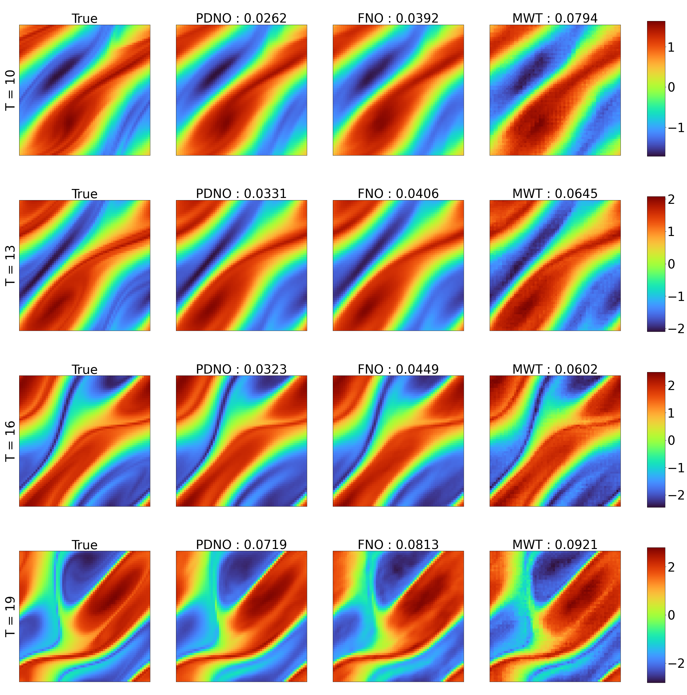
Figure 10: Comparison the prediction on Navier-Stokes equation with $\nu=1e-5$. This test sample shows the lowest relative $L^{2}$ error on average of three models.

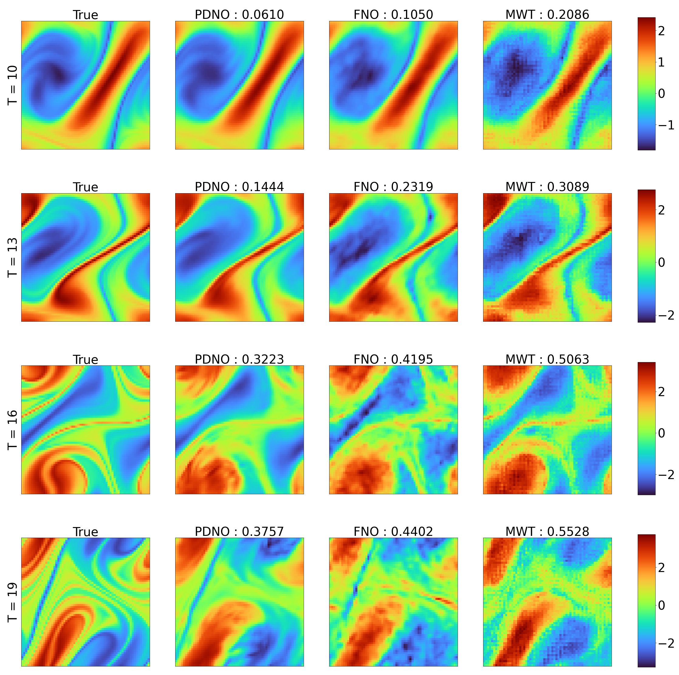
Figure 11: Comparison the prediction on Navier-Stokes equation with $\nu=1e-5$. This test sample shows the greatest relative $L^{2}$ error on average of three models.

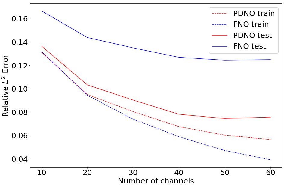
Figure 12: Training and test error of the proposed model and FNO on Navier-Stokes data with $\nu=1e-5$ according to the number of channels.

References

- [1] Saakaar Bhatnagar, Yaser Afshar, Shaowu Pan, Karthik Duraisamy, and Shailendra Kaushik. Prediction of aerodynamic flow fields using convolutional neural networks. Comput. Mech., 64(2):525–545, 2019.
- [2] Louis Boutet de Monvel. Boundary problems for pseudo-differential operators. Acta Math., 126(1-2):11–51, 1971.
- [3] Tianping Chen and Hong Chen. Universal approximation to nonlinear operators by neural networks with arbitrary activation functions and its application to dynamical systems. IEEE Transactions on Neural Networks, 6(4):911–917, 1995.
- [4] R. Courant and D. Hilbert. Methods of mathematical physics. Vol. I. Interscience Publishers, Inc., New York, N.Y., 1953.
- [5] J. J. Duistermaat. Fourier integral operators, volume 130 of Progress in Mathematics. Birkhäuser Boston, Inc., Boston, MA, 1996.
- [6] J. J. Duistermaat and L. Hörmander. Fourier integral operators. II. Acta Math., 128(3-4):183–269, 1972.
- [7] Weinan E and Bing Yu. The deep Ritz method: a deep learning-based numerical algorithm for solving variational problems. Commun. Math. Stat., 6(1):1–12, 2018.
- [8] Xavier Glorot, Antoine Bordes, and Yoshua Bengio. Deep sparse rectifier neural networks. In Proceedings of the fourteenth international conference on artificial intelligence and statistics, pages 315–323. JMLR Workshop and Conference Proceedings, 2011.
- [9] Xiaoxiao Guo, Wei Li, and Francesco Iorio. Convolutional neural networks for steady flow approximation. In Proceedings of the 22nd ACM SIGKDD international conference on knowledge discovery and data mining, pages 481–490, 2016.
- [10] Gaurav Gupta, Xiongye Xiao, and Paul Bogdan. Multiwavelet-based operator learning for differential equations. Advances in Neural Information Processing Systems, 34, 2021.
- [11] Jan S Hesthaven, Sigal Gottlieb, and David Gottlieb. Spectral methods for time-dependent problems, volume 21. Cambridge University Press, 2007.
- [12] Philipp Holl, Vladlen Koltun, and Nils Thuerey. Learning to control pdes with differentiable physics. arXiv preprint arXiv:2001.07457, 2020.
- [13] Lars Hörmander. Fourier integral operators. I. Acta Math., 127(1-2):79–183, 1971.
- [14] Lars Hörmander. The analysis of linear partial differential operators. I. Classics in Mathematics. Springer-Verlag, Berlin, 2003. Distribution theory and Fourier analysis, Reprint of the second (1990) edition [Springer, Berlin; MR1065993 (91m:35001a)].
- [15] Lars Hörmander. The analysis of linear partial differential operators. III. Classics in Mathematics. Springer, Berlin, 2007. Pseudo-differential operators, Reprint of the 1994 edition.
- [16] Hyung Ju Hwang, Jin Woo Jang, Hyeontae Jo, and Jae Yong Lee. Trend to equilibrium for the kinetic Fokker-Planck equation via the neural network approach. J. Comput. Phys., 419:109665, 25, 2020.
- [17] Rakhoon Hwang, Jae Yong Lee, Jin Young Shin, and Hyung Ju Hwang. Solving pde-constrained control problems using operator learning. arXiv preprint arXiv:2111.04941, 2021.
- [18] Yuehaw Khoo, Jianfeng Lu, and Lexing Ying. Solving parametric PDE problems with artificial neural networks. European J. Appl. Math., 32(3):421–435, 2021.
- [19] Georgios Kissas, Jacob Seidman, Leonardo Ferreira Guilhoto, Victor M Preciado, George J Pappas, and Paris Perdikaris. Learning operators with coupled attention. arXiv preprint arXiv:2201.01032, 2022.
- [20] Jae Yong Lee, Jin Woo Jang, and Hyung Ju Hwang. The model reduction of the Vlasov-Poisson-Fokker-Planck system to the Poisson-Nernst-Planck system via the deep neural network approach. ESAIM Math. Model. Numer. Anal., 55(5):1803–1846, 2021.
- [21] Zongyi Li, Nikola Kovachki, Kamyar Azizzadenesheli, Burigede Liu, Kaushik Bhattacharya, Andrew Stuart, and Anima Anandkumar. Fourier neural operator for parametric partial differential equations. arXiv preprint arXiv:2010.08895, 2020.
- [22] Zongyi Li, Nikola Kovachki, Kamyar Azizzadenesheli, Burigede Liu, Kaushik Bhattacharya, Andrew Stuart, and Anima Anandkumar. Multipole graph neural operator for parametric partial differential equations. arXiv preprint arXiv:2006.09535, 2020.
- [23] Zongyi Li, Nikola Kovachki, Kamyar Azizzadenesheli, Burigede Liu, Kaushik Bhattacharya, Andrew Stuart, and Anima Anandkumar. Neural operator: Graph kernel network for partial differential equations. arXiv preprint arXiv:2003.03485, 2020.
- [24] Lu Lu, Pengzhan Jin, and George Em Karniadakis. Deeponet: Learning nonlinear operators for identifying differential equations based on the universal approximation theorem of operators. arXiv preprint arXiv:1910.03193, 2019.
- [25] Mohammad Amin Nabian and Hadi Meidani. A deep neural network surrogate for high-dimensional random partial differential equations. arXiv preprint arXiv:1806.02957, 2018.
- [26] M. Raissi, P. Perdikaris, and G. E. Karniadakis. Physics-informed neural networks: a deep learning framework for solving forward and inverse problems involving nonlinear partial differential equations. J. Comput. Phys., 378:686–707, 2019.
- [27] Prajit Ramachandran, Barret Zoph, and Quoc V Le. Searching for activation functions. arXiv preprint arXiv:1710.05941, 2017.
- [28] Michael Reed and Barry Simon. Methods of modern mathematical physics. I. Functional analysis. Academic Press, New York-London, 1972.
- [29] Michael Ruzhansky and Ville Turunen. Pseudo-differential operators and symmetries: background analysis and advanced topics, volume 2. Springer Science & Business Media, 2009.
- [30] Justin Sirignano and Konstantinos Spiliopoulos. DGM: a deep learning algorithm for solving partial differential equations. J. Comput. Phys., 375:1339–1364, 2018.
- [31] Michael Eugene Taylor. Pseudodifferential Operators (PMS-34). Princeton University Press, 2017.
- [32] Sifan Wang, Hanwen Wang, and Paris Perdikaris. Learning the solution operator of parametric partial differential equations with physics-informed deeponets. arXiv preprint arXiv:2103.10974, 2021.
- [33] Yinhao Zhu and Nicholas Zabaras. Bayesian deep convolutional encoder-decoder networks for surrogate modeling and uncertainty quantification. J. Comput. Phys., 366:415–447, 2018.
- [34] Yinhao Zhu, Nicholas Zabaras, Phaedon-Stelios Koutsourelakis, and Paris Perdikaris. Physics-constrained deep learning for high-dimensional surrogate modeling and uncertainty quantification without labeled data. J. Comput. Phys., 394:56–81, 2019.