Wassersplines for Neural Vector Field–Controlled Animation

Abstract

Much of computer-generated animation is created by manipulating meshes with rigs. While this approach works well for animating articulated objects like animals, it has limited flexibility for animating less structured free-form objects. We introduce Wassersplines, a novel trajectory inference method for animating unstructured densities based on recent advances in continuous normalizing flows and optimal transport. The key idea is to train a neurally-parameterized velocity field that represents the motion between keyframes. Trajectories are then computed by advecting keyframes through the velocity field. We solve an additional Wasserstein barycenter interpolation problem to guarantee strict adherence to keyframes. Our tool can stylize trajectories through a variety of PDE-based regularizers to create different visual effects. We demonstrate our tool on various keyframe interpolation problems to produce temporally-coherent animations without meshing or rigging.

<ccs2012> <concept> <concept_id>10010147.10010371.10010352.10010380</concept_id> <concept_desc>Computing methodologies Motion processing</concept_desc> <concept_significance>500</concept_significance> </concept> <concept> <concept_id>10010147.10010371.10010396.10010400</concept_id> <concept_desc>Computing methodologies Point-based models</concept_desc> <concept_significance>300</concept_significance> </concept> </ccs2012>

[500]Computing methodologies Motion processing [300]Computing methodologies Point-based models

1 Introduction

In hand-drawn animation, a primary artist is tasked with laying out keyframes. These frames define the rough motion of an animation and occupy a fraction of the usual 12 drawings per second. The remaining frames are filled in afterwards to create smooth motion in a process called inbetweening. In the transition from hand-drawn animation to computer-assisted animation, much of the inbetweening process became automated [Las87]. After an artist lays out keyframes as mesh rig displacements, in-between frames can be produced automatically using splines and other interpolation machinery. Secondary effects like elastic oscillation or fluids can be added afterwards through physical simulation [KA08]. This process is largely responsible for modern character animation and has had major success for articulated objects like humans and animals.

While methods for articulated animation via meshes and rigs are abundant, research on animation of objects like the Drunn in Walt Disney Animation Studio’s “Raya and the Last Dragon” is far less common. These animations are characterized by abstract, amorphous boundaries and free-form motion. As with classical animation, keyframes are still provided by an artist to coarsely define the desired motion. Due to the lack of structure between keyframes, however, we denote such animations as unstructured. Rig-based methods are insufficient in this case, since unstructured animations can separate and recombine. Simultaneous to their freedom of movement, their trajectories must accurately reach keyframes, so that an artist is able to convey the appropriate gestures in a scene.

Unstructured animation can be found in various media over the last several decades. In 1991, “Terminator 2: Judgment Day” depicts visual effects of mercury transitioning into various geometries. The unstructured animation style even pre-dates computer animation and can be found in the exaggerated motions of Cruella’s cigarette smoke in Disney’s 1961 “One Hundred and One Dalmations.” That is to say, interest in this type of animation is abundant, but methods are largely manual, highly specific to the scene, and undocumented.

In this paper, we present Wassersplines for unstructured animation. We encode keyframes as point clouds or probability measures, allowing us to capture arbitrary geometries without the limitations of a mesh or rig. Trajectories are encoded using a coordinate multi-layer perceptron (MLP) to produce a velocity field in space-time. A rough animation is then produced by advecting points through the velocity field. We propose a Wasserstein barycenter interpolation step to guarantee strict keyframe adherence. Using partial differential equation– (PDE–) based regularizers on the coordinate MLP, we bring about various effects in the animation without needing extra keyframes. We demonstrate our method on 2D and 3D examples, showing strict adherence to keyframes and flexibility in the interpolations.

2 Related Work

Normalizing Flows.

Normalizing flows map a prescribed initial density, such as a Gaussian, through a set of invertible functions to a target posterior distribution [RM15, PNR*21]. Neural ordinary differential equations (ODE) take this concept to the limit by parameterizing the state derivative with a deep neural network. Continuous normalizing flows (CNF) integrate the neural ODE to produce the target posterior distribution [CRBD18]. In this context, [GCB*18] use the Hutchinson’s trace estimator to compute posterior density values through a neural ODE.

Various strategies decrease training time for CNFs. [KBJD20, FJNO20] regularize the spatial variation of the state derivative and its higher-order time derivatives. [TSM*20] use random Fourier features (RFF) for faster training of high-frequency state derivatives. [HPG*21] sequentially unmask RFFs in order of increasing frequency, decreasing sensitivity to the initial RFF sampling. [PMY*20] learn auxiliary networks for faster ODE integration, a costly step in application of CNFs.

Optimal Transport.

Optimal transport (OT) models compute the cheapest map from a source distribution onto a target distribution via a linear program [Kan06]. The cost of this map defines the Wasserstein distance between distributions; see [PC*19, Sol18, San15] for general discussion.

Adding entropic regularization to the optimal transport linear program yields an efficient and easily-implemented optimization technique known as Sinkhorn’s algorithm or matrix rebalancing [Cut13]. While cheaper to compute, entropically-regularized optimal transport biases the Wasserstein metric so that the distance from a distribution to itself is nonzero. This issue is fixed in the definition of the Sinkhorn divergence by adding a de-biasing term to entropic optimal transport [GPC18]. Efficient large-scale implementations of Sinkhorn divergence and other optimal transport routines are available through “GeomLoss” [FSV*19] and “POT: Python Optimal Transport” [FCG*21].

Dynamical optimal transport provides an alternative means of computing Wasserstein distances when the ground metric is quadratic in geodesic distance. Instead of computing a map between the source and target distributions, it computes a kinetic energy-minimizing velocity field that advects the source distribution into the target [BB00]; recent algorithms accelerate solution of the relevant variational problems and explore alternative mesh-based and neural parameterizations [LCCS18, Lav21, PPO14, THW*20].

Image/Shape Registration.

Registrations between images or shapes can be built from velocity field–induced diffeomorphisms. [HMP15] regularize the velocity field in dynamical optimal transport and prove existence of minimizers with a velocity gradient regularizer. [ELC19] compute static volume-preserving, velocity fields for mesh registration. [FCVP17] use unbalanced OT to build diffeomorphic registrations in medical imaging.

Measure-valued Splines.

Higher-order interpolations can be computed through an ordered sequence of distributions by minimizing acceleration instead of kinetic energy [CCG18, BGV19]. [BGV19] compute solutions as distributions over cubic splines via a multi-marginal transport problem. [CCL*21] show that such solutions do not allow for deterministic trajectory inference and instead compute optimal transport plans between consecutive pairs of point clouds followed by classical spline interpolation.

Our problem also aims to interpolate an input sequence of distributions. A major difference, however, is that we parameterize the trajectory of our interpolation with a velocity field. This difference allows us to regularize based on spatial derivatives of the velocity rather than just time-derivatives like acceleration. Furthermore, our aim is not to globally minimize any particular time derivative but rather to provide a palette of effects to control a trajectory.

Trajectory Inference.

[SST*19, LZKS21] propose Waddington OT for inference of cellular dynamics by concatenating OT interpolations between consecutive keyframes. The approach used by [Ric21] to animate Drunn is similar in that it also computes OT matchings between consecutive point clouds. A key difference, however, is that the point clouds used in animation of Drunn are automatically generated by sampling densities evolved via fluid simulation. This provides an abundance of data, mitigating artifacts of the piecewise-smooth trajectory. [TCCS21, TMPS03, PM17] augment incompressible fluid simulations with additional forces to interpolate between target keyframes. These methods balance between proximity to keyframes and regularization of additional forces thus allowing deviation from target keyframes. [BBRF14] interpolate keyframes by matching image patches between keyframes. To get smoother trajectories, however, they also allow deviation from the provided keyframes.

3 Preliminaries

For completeness, we overview relevant developments in continuous normalizing flows and optimal transport. For detailed coverage, see [PNR*21, PC*19, GPC18].

3.1 Neural ODEs and CNFs

CNFs fit a target measure as the pushforward of a source measure through a diffeomorphism, granting users the ability to sample the target measure as long as they have sample access to the source measure. We will re-purpose tools from the CNF literature to generate unstructured animations and review their basics here.

Given an initial state $z(t_{0})\in\mathbb{R}^{n}$ and parameterized state derivative function $f_{\theta}(z,t)\in\mathbb{R}^{n}$, one can solve the ODE $\dot{z}=f_{\theta}(z,t)$ for $z$ at time $t_{1}$ as

$$z(t_{1})=z(t_{0})+\int_{t_{0}}^{t_{1}}f_{\theta}(z(t),t)dt.$$ (1)

When $f_{\theta}(z,t)$ is parameterized by a deep neural network, it is referred to as a coordinate MLP; $\dot{z}=f_{\theta}(z,t)$ is a neural ODE. Given a loss function $L(z(t_{1}))$, the gradient $\nabla_{\theta}L(z(t_{1}))$ is computed by the adjoint method using black box ODE solvers [CRBD18].

Neural ODEs build CNFs in the following way. Let $\nu$ be a source measure with simple parametric density on $\mathbb{R}^{n}$, $\mu$ be the measure of a target density, and $\phi$ be a map from $z(t_{0})$ to $z(t_{1})$. Then $\phi_{\#}\nu$ denotes the pushforward measure obtained by advecting $\nu$ through $f_{\theta}$ from $t_{0}$ to $t_{1}$, i.e., the pushforward of $\nu$ by $\phi$. The CNF generating $\mu$ is obtained by minimizing Kullback-Leibler (KL) divergence $\text{KL}(\mu|\phi_{\#}\nu)$ with

$$\text{KL}(p|q)=\int_{\mathbb{R}^{n}}\log\left(\frac{dp}{dq}\right)dp$$ (2)

for measures $p$, $q$ over $\mathbb{R}^{n}$ [PNR*21, CRBD18].

3.2 From Wasserstein Distance to Sinkhorn Divergence

While KL divergence is a popular loss function for building CNFs, it requires overlapping support and density access to work. To bypass these shortcomings, we use Sinkhorn Divergence instead and introduce it here.

Given probability measures $\mu$ and $\nu$ on $\mathcal{X}\subset\mathbb{R}^{n}$, let $\Pi(\mu,\nu)$ denote the set of joint probability measures on $\mathcal{X}\times\mathcal{X}$ with marginals $\mu$ and $\nu$. The squared 2-Wasserstein distance between $\mu$ and $\nu$ is defined as

$$W_{2}^{2}(\mu,\nu):=\inf_{\pi\in\Pi(\mu,\nu)}\int_{\mathcal{X}\times\mathcal{X}}\|x-y\|^{2}d\pi(x,y).$$ (3)

The joint probability measure solving Equation 3 is the optimal transport plan $\pi$. The 2-Wasserstein distance is well defined even when $\mu$ and $\nu$ are non-overlapping, and its gradient brings non-overlapping measures together.

Equation 3 is computationally challenging to solve, leading to the popular use of entropic regularization. Entropically-regularized transport distance is defined via the convex program

$$\text{OT}_{\epsilon}(\mu,\nu):=\inf_{\pi\in\Pi(\mu,\nu)}\int_{\mathcal{X}\times\mathcal{X}}\|x-y\|^{2}d\pi(x,y)+\epsilon KL(\pi\mid\mu\otimes\nu).$$ (4)

Unlike Equation 3, $\text{OT}_{\epsilon}(\mu,\nu)$ can be computed efficiently by Sinkhorn’s algorithm [Cut13]. This efficiency comes at the cost of entropic bias, i.e., $\text{OT}_{\epsilon}(\mu,\mu)\neq 0$. The bias becomes especially problematic when one is interested in Wasserstein gradient flows to transform a source measure $\nu$ into a target measure $\mu$. One could implement the flow $\dot{\nu}=-\nabla_{\nu}OT_{\epsilon}(\mu,\nu)$, but it would converge to a solution where $\nu\neq\mu$ [FSV*19]. To address this bias, [GPC18] build the Sinkhorn divergence:

$$S_{\epsilon}(\mu,\nu):=\text{OT}_{\epsilon}(\mu,\nu)-\frac{1}{2}\text{OT}_{\epsilon}(\mu,\mu)-\frac{1}{2}\text{OT}_{\epsilon}(\nu,\nu).$$ (5)

$S_{\epsilon}(\mu,\nu)$ eliminates entropic bias and restores the desired property $S_{\epsilon}(\mu,\mu)=0$. When $\epsilon=0$, we have the equivalence

$$S_{0}(\mu,\nu)=\text{OT}_{0}(\mu,\nu)=W_{2}^{2}(\mu,\nu),$$

but the computational benefits of entropic transport are lost.

3.3 Unbalanced Optimal Transport

Unbalanced optimal transport is an extension of OT where marginal constraints are softened and controlled by an extra parameter $\tau$. The softened constraints make unbalanced OT more robust to outliers, which we use in §6 to improve quality of results. Let $\mathcal{M}^{+}(\mathcal{X}\times\mathcal{X})$ be the space of positive measures on $\mathcal{X}\times\mathcal{X}$. Then the unbalanced OT cost is

$$\text{OT}_{\epsilon,\tau}(\mu,\nu) :=\inf_{\pi\in\mathcal{M}^{+}(\mathcal{X}\times\mathcal{X})}\int_{\mathcal{X}\times\mathcal{X}}\|x-y\|^{2}d\pi(x,y)$$

$$+\epsilon KL(\pi\mid\mu\otimes\nu)+\tau^{2}KL(\pi_{1}\mid\mu)+\tau^{2}KL(\pi_{2}\mid\nu),$$ (6)

where $\pi_{1}$ and $\pi_{2}$ are marginals of $\pi$ [Fey20], and $\tau$ can be intuitively thought of as the maximum distance a piece of mass can be transported before the transport plan $\pi$ would rather violate marginal constraints. $\tau$ is referred to as “reach” in GeomLoss [FCVP17, FSV*19].

Unbalanced Sinkhorn divergence $S_{\epsilon,\tau}$ is defined exactly the same as $S_{\epsilon}$ in Equation 5 but with $\text{OT}_{\epsilon}$ replaced by $\text{OT}_{\epsilon,\tau}$. Despite the softening of marginal constraints, $S_{\epsilon,\tau}(\mu,\nu)=0$ still implies $\mu=\nu$. When, $\tau=\infty$, $S_{\epsilon,\tau}=S_{\epsilon}$ i.e. balanced Sinkhorn divergence.

4 Method

We now present unstructured animation as a measure interpolation problem equipped with a suitable fitting loss. We describe how to control the animation through different regularizers as well as how to guarantee strict adherence to keyframes.

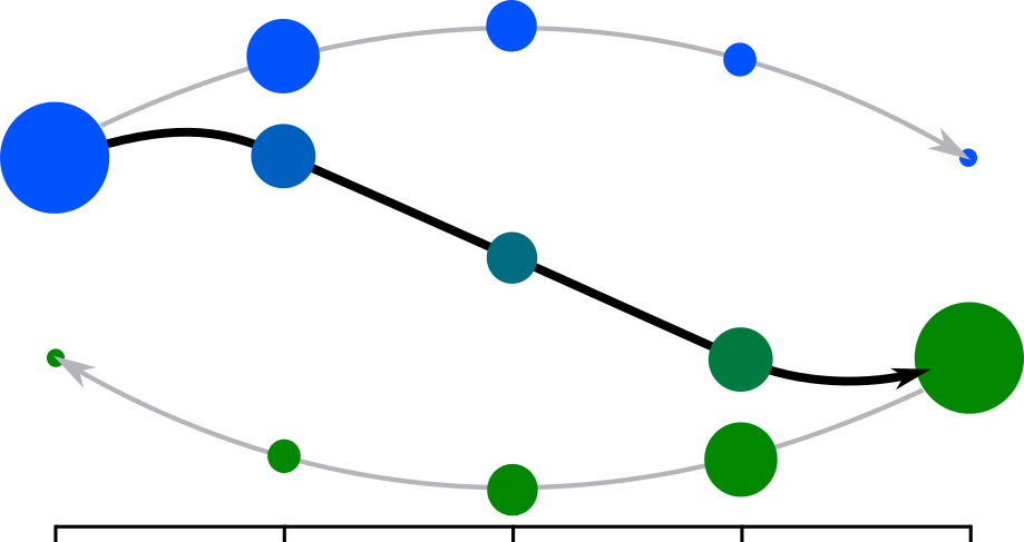
Figure 1: Schematic of Wasserstein barycenter interpolation. While the neural ODE–produced trajectories (in grey) do not precisely adhere to keyframes, the modified trajectory produced using Equation 20 (in black) is guaranteed to adhere to keyframes.

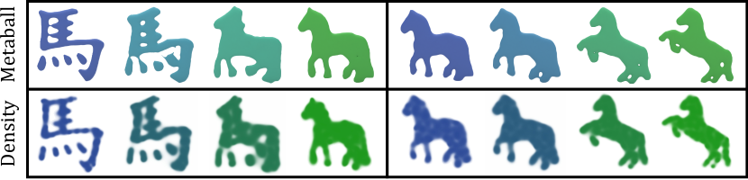
Figure 2: Different renderings of our results. The first row is rendered by converting point clouds into an explicit surface using metaballs with a 0.05 radius. This technique results in more well defined boundaries but less visible interior density variation. The second row is rendered directly as densities computed via [BVPH11]. Boundaries are less sharp. but more interior variation is revealed.

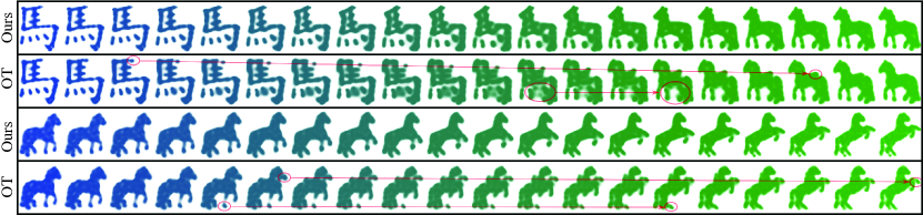
Figure 3: Comparison between trajectories obtained using our method and optimal transport for interpolating between the Chinese character for “horse” and an image of a horse (rows 1 and 2) and between two images of horses in different poses (rows 3 and 4). The OT interpolation computed via [FCG*21] exhibits more spatial discontinuities (circled in red).

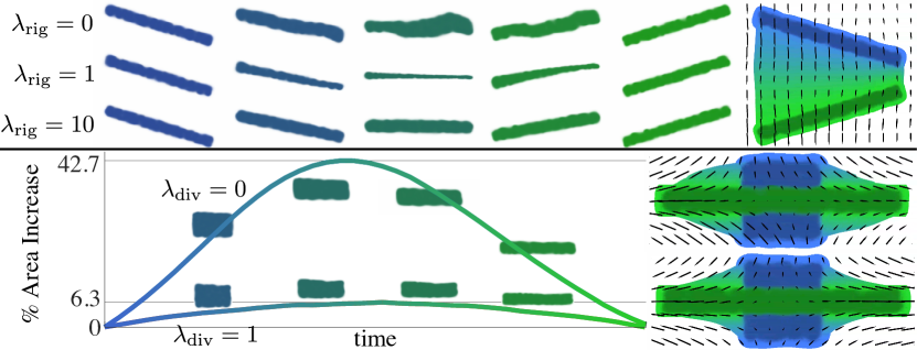
Figure 4: Effect of rigidity and compressibility regularization on our trajectories. Increasing the coefficient of the rigidity regularizer yields a less wobbly interpolation between two straight bars (top). Regularizing compressibility when interpolating between a square and rectangle reduces the increase in area of the shapes along the trajectory (bottom).

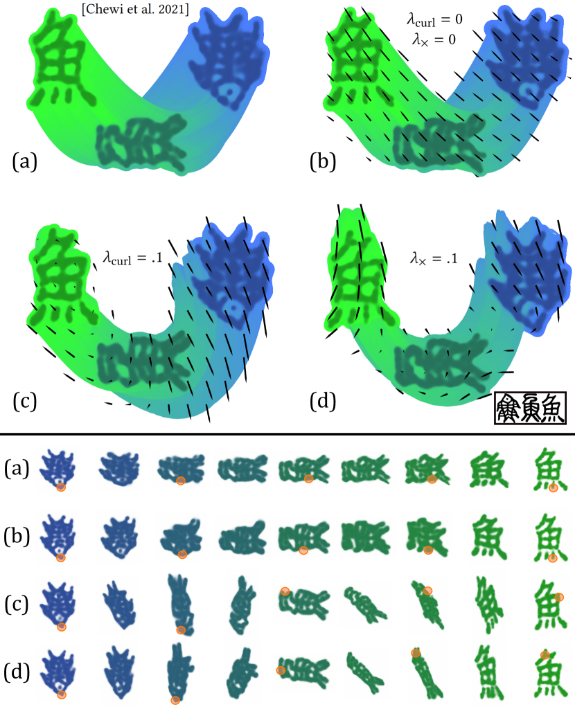
Figure 5: Interpolation between three keyframes, demonstrating the evolution of the Chinese character for “fish.” Without swirliness regularization ($\lambda_{\text{curl}}=\lambda_{\times}=0$), the character does not properly rotate, with the head of the fish in the first keyframe (circled in orange) getting mapped to the tail in the last. Trajectories using [CCL*21] exhibit the same issue. When we regularize the trajectory with $\lambda_{\text{curl}}=10^{-1}$, the head of the fish in the first keyframe over-rotates, landing near the head of the final keyframe. When regularizing with $\lambda_{\times}=10^{-1}$, the head of the fish in the first keyframe is properly mapped to the head of the fish in the last keyframe.

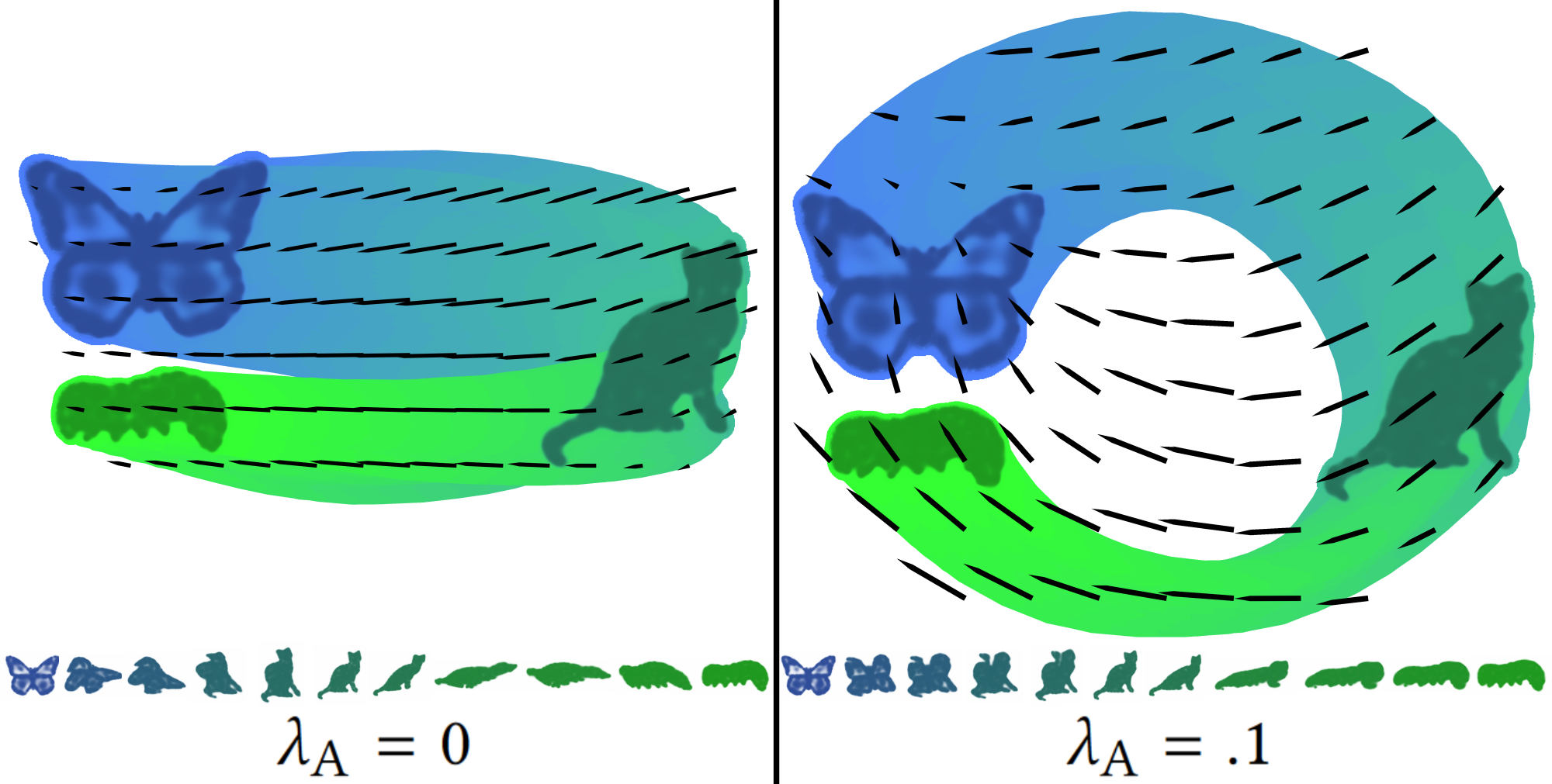
Figure 6: Effect of user-directed alignment on our trajectories. Adding this regularizer (right) to the original trajectory (left) yields a more circuitous path.

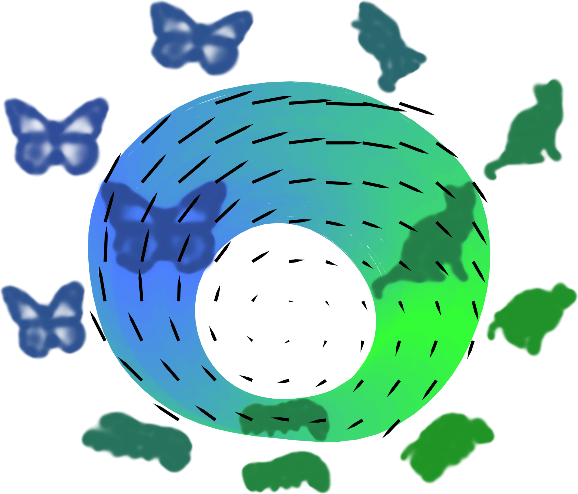
Figure 7: By combining user-directed alignment and carefully chosen Fourier frequencies we compute perfectly loopable circular trajectories depicting the fictitious lifecycle of a butterfly.

Figure 8: Effects of various regularizers on a four-keyframe animation. Employing rigidity, user-directed alignment, acceleration, and swirliness regularization as well as modifying the standard deviation of the RFF results in trajectories with varying path qualities and shapes. We also compare to trajectories obtained using optimal transport [FCG*21] and [CCL*21].

4.1 Notation

Let the keyframes be the set $\mathcal{K}=\{(\mathcal{X}_{i},t_{i})\}_{i=0}^{T-1}$, where each $\mathcal{X}_{i}$ is a measure over $\mathbb{R}^{d}$ for $d\in\{2,3\}$ from which we can draw samples; $t_{i}$ are corresponding timestamps. Similarly to [THW*20], we compute trajectories between keyframes using a coordinate MLP

$$f_{\theta}(z,t):\mathbb{R}^{d}\times\mathbb{R}\rightarrow\mathbb{R}^{d}$$ (7)

and neural ODE $\dot{z}=f_{\theta}(z,t)$. This choice gives us easy access to all derivatives of $f_{\theta}$, something that would be more limited under a non-neural parameterization, e.g., if we parameterize $f_{\theta}$ on a grid with piecewise tri-linear basis functions, $\ddot{f_{\theta}}=0$.

For times $t_{i}\leq t_{j}$, let $\phi^{t_{i},t_{j}}$ be the diffeomorphism of $\mathbb{R}^{d}$ resulting from integrating (7) from time $t_{i}$ to time $t_{j}$. When $t_{i}>t_{j}$, $\phi^{t_{i},t_{j}}$ is the inverse of $\phi^{t_{j},t_{i}}$. Let $\mathcal{X}_{i}^{t_{j}}$ be shorthand for the pushforward of keyframe $\mathcal{X}_{i}$ by $\phi^{t_{i},t_{j}}$:

$$\mathcal{X}_{i}^{t_{j}}=\phi^{t_{i},t_{j}}_{\#}\mathcal{X}_{i}.$$ (8)

We sample from $\mathcal{X}_{i}^{t_{j}}$ by evolving samples from $\mathcal{X}_{i}$ through the ODE (1) from time $t_{i}$ to time $t_{j}$. In this notation, a trajectory strictly adhering to keyframes satisfies

$$\mathcal{X}_{i}^{t_{j}}=\mathcal{X}_{j}.$$ (9)

4.2 Fitting Loss

CNF methods like [THW*20, CRBD18, GCB*18] use Kullback-Leibler divergence $\text{KL}(\mathcal{X}_{j}|\mathcal{X}_{i}^{t_{j}})$ as a fitting loss. For unstructured animation, however, a KL loss is unsuitable because animation keyframes often have compact support; in particular, pushforward measures like $\mathcal{X}_{i}^{t_{j}}$ are unlikely to overlap with their targets $\mathcal{X}_{j}$ early in training. Furthermore, computing KL divergence requires density access, which is expensive to estimate. These situations leave the KL divergence undefined or infinite [ACB17].

Instead, we use Sinkhorn divergence as a trajectory fitting loss:

$$L_{\text{fit}}^{i,j}=S_{\epsilon}(\mathcal{X}_{i}^{t_{j}}|\mathcal{X}_{j}).$$ (10)

A Sinkhorn divergence of exactly 0 guarantees that $\mathcal{X}_{i}^{t_{j}}=\mathcal{X}_{j}$. Unlike KL divergence, Sinkhorn divergence has no dependence on overlapping support between its measures. In addition, its gradient brings non-overlapping measures together. Finally, Sinkhorn divergence can be computed with only sample access from its input measures.

Our total trajectory fitting loss is then

$$L_{\text{fit}}=\sqrt{\sum_{i=0}^{T-2}L_{\text{fit}}^{i,i+1}+L_{\text{fit}}^{i+1,i}}.$$ (11)

This choice is motivated by “teacher-forcing” in training recurrent neural networks (RNNs), where one inserts ground-truth data into the network to decrease training time [WZ89]. In our case, $L_{\text{fit}}$ is constructed by evaluating Equation 10 only between consecutive keyframes, i.e., the ground truth data. We also use a square root in Equation 11 in preparation to balance our fitting loss against a regularization energy. Recall that $L_{\text{fit}}^{i,i+1}$ is essentially a squared Wasserstein distance and that gradients of squared quantities decrease with the magnitudes of their arguments. The square-root maintains the magnitude of the fitting loss gradient even as the fitting loss approaches 0. This ensures that fitting loss gradients are not out-competed by regularizers.

4.3 Controlling the Trajectory

Within the space of trajectories that minimize the fitting loss, we can encourage paths with desirable features by regularizing the velocity field $f_{\theta}$. This process is straightforward, since types of motion have natural vector calculus or continuum mechanics counterparts. Here, we identify different types of motion with mathematical quantities based on vector field $f_{\theta}$ in a pointwise manner. These pointwise quantities will be denoted $l_{\square}$ with placeholder symbol $\square$. We then show how to integrate these pointwise quantities in space-time to build a corresponding regularizing loss $L_{\square}$. These regularizers enable the user to select from a palette of options to control their animation.

Squash and Stretch.

We begin with one of the basic principles of animation: “squash and stretch” [TJT95]. A mathematical measure for this type of movement is rigidity:

$$l_{\text{rig}}=\|\nabla_{z}f_{\theta}+\nabla_{z}f_{\theta}^{\top}\|_{F}^{2},$$ (12)

where $\|\cdot\|_{F}$ denotes Frobenius norm. This term can also be interpreted as a Killing vector field energy [BBSG10], or, from the perspective of continuum mechanics, $f_{\theta}$ is the displacement gradient, and $l_{\text{rig}}$ is the magnitude of the linear strain tensor. Movements generated by a velocity field where $l_{\text{rig}}=0$ will appear rigid and not squash or stretch keyframes.

Compressibility.

A closely related concept to rigidity is compressibility. Consider a quivering block of gelatin. While its movements are non-rigid, squashing in height will cause bulging in width. Compressibility can be captured by divergence:

$$l_{\text{div}}=(\nabla\cdot f_{\theta})^{2}=\text{Tr}[\nabla_{z}f_{\theta}]^{2}.$$ (13)

Movements of a keyframe generated by a velocity field where $l_{\text{div}}=0$ will preserve area or volume, i.e., they are incompressible.

User-Directed Alignment.

We can explicitly incentivize keyframes to move in certain directions during the animation via a user-provided metric $A(z,t)\in\mathbb{R}^{d\times d}$ by minimizing

$$l_{\text{A}}=\|f_{\theta}\|_{A}^{2}=f_{\theta}^{\top}Af_{\theta}.$$ (14)

If the user wants $f_{\theta}$ to align with unit vector field $v$, they can choose the metric $A=I-vv^{\top}$. Conversely, the user can also penalize alignment of $f_{\theta}$ to $v$ with $A=vv^{\top}$.

Swirliness.

One of the most visually salient features of an animation or fluid is its swirliness. This is naturally captured by vector valued quantity curl: $\nabla\times f_{\theta}$. Its direction points in the axis of rotation, and its magnitude is twice the angular velocity. Given a target curl vector $\vec{c}$, we can quantify how close $f_{\theta}$ is to meeting that target with

$$l_{\text{curl}}=\|\nabla\times f_{\theta}-\vec{c}\|_{2}^{2}.$$ (15)

For example, if we want a 2D animation where the keyframe rotates a full circle clockwise in four seconds, then we can measure $l_{\text{curl}}$ with $\vec{c}=[0,0,-\pi]^{\top}$.

$l_{\text{curl}}$ allows us to quantify how much $f_{\theta}$ deviates from the target curl at any specific point in the trajectory. To quantify how much the integrated curl vector along a trajectory deviates from the target, we also need $l_{\times}=\nabla\times f_{\theta}$, the only vector valued $l_{\square}$ in our list of regularizers.

Smoothness.

Finally, we mention some regularizers from the neural ODE literature. ODE solvers can be slow to converge if $f_{\theta}$ varies too much spatially or temporally [KBJD20, FJNO20]. One can try to make $f_{\theta}$ smoother with the following:

$$l_{\text{grad}}=\|\nabla_{z}f_{\theta}\|_{F}^{2},\hfill$$ (16)

$$l_{\text{vel}}=\|f_{\theta}\|_{2}^{2},\;\;l_{\text{acc}}=\|\dot{f_{\theta}}\|_{2}^{2},\;\;l_{\text{jerk}}=\|\ddot{f_{\theta}}\|_{2}^{2}.$$ (17)

$l_{\text{grad}}$ quantifies spatial variation of $f_{\theta}$, while $l_{\text{vel}}$, $l_{\text{acc}}$, and $l_{\text{jerk}}$ measure orders of temporal variation, i.e., speed, acceleration, and jerk.

Integrating Along the Trajectory.

We have defined various point-wise quantities based on $f_{\theta}$. We will denote all of them with $l_{\square}(z,t)$, where $\square$ can be replaced with any of the previously-mentioned quantities. To regularize $f_{\theta}$ with $l_{\square}(z,t)$ we use the loss

$$L_{\square}=\frac{1}{2}\sum_{i=0}^{T-2}\int_{t_{i}}^{t_{i+1}}\int_{\mathbb{R}^{d}}l_{\square}(z,t)d\left(\mathcal{X}_{i}^{t}+\mathcal{X}_{i+1}^{t}\right)dt$$ (18)

that integrates $l_{\square}$ over the trajectory dictated by $f_{\theta}$. As with Equation 11, Equation 18 only considers trajectories obtained by flowing keyframes to their consecutive neighbors. Doing this avoids applying regularization unnecessarily at space-time locations that come from accumulated error in ODE integration.

We add regularizer $L_{\square}$ to our total loss with coefficient $\lambda_{\square}$. The one exception to this symbolic grouping ($\lambda_{\square}$, $L_{\square}$) is when $\square=\times$ because $L_{\times}$ is a vector. Let $\lambda_{\times}$ represent regularizing factor corresponding to regularizing loss function $\|L_{\times}-\vec{c}\|^{2}_{2}$ with target curl $\vec{c}$. $\lambda_{\times}$ regularizes the average curl as opposed to $\lambda_{\text{curl}}$ which regularizes pointwise curl. We show in §6 the isolated effects of these regularizers and how they can be used to control an animation. The total loss function is

$$L_{\text{tot}}=L_{\text{fit}}+\sum_{\text{scalars}}\lambda_{\square}L_{\square}+\lambda_{\times}\|L_{\times}-\vec{c}\|_{2}^{2}$$ (19)

4.4 Wasserstein Barycenter Interpolation

After training the neural ODE, we are not yet guaranteed that the trajectory strictly adheres to keyframes, as the neural ODE balances the fitting loss and regularizing losses. If $L_{\text{fit}}\neq 0$, the neural ODE trajectories deviate from keyframes. We correct deviation by applying the following Wasserstein barycenter interpolation step. Given a query time $t\in[t_{i},t_{i+1}]$, our output in-between frame is defined as

$$\vspace{-3pt}\mathcal{X}_{\epsilon,\tau}(t)=\text{argmin}_{\alpha}\left(t_{i+1}-t\right) S_{\epsilon,\tau}(\mathcal{X}_{i}^{t},\alpha)$$

$$+\left(t-t_{i}\right) S_{\epsilon,\tau}(\alpha,\mathcal{X}_{i+1}^{t}).\vspace{-1pt}$$ (20)

In this way, our output trajectories are guaranteed to adhere to the keyframes: $\mathcal{X}_{\epsilon,\tau}(t_{i})=\mathcal{X}_{i}$ for any choice of $\epsilon$ and $\tau$. This step of our pipeline is similar to [SDP*15], who use Wasserstein barycenters for shape interpolation, but their barycenters are computed directly between keyframes while our barycenters are computed between ODE-advected keyframes allowing for artistic control. When $L_{\text{fit}}=0$, Equation 20 becomes trivial with $\mathcal{X}(t)=\mathcal{X}_{i}^{t}=\mathcal{X}_{i+1}^{t}$. Our interpolation is illustrated schematically in Figure 1.

5 Implementation Details

Here we describe various implementation details needed to replicate our results. The majority of figures are produced with the same default parameters though our method is not overly sensitive to these choices.

Keyframes have been presented so far as measures over $\mathbb{R}^{d}$ with sample access. Our implementation mirrors this assumption and samples $N$ points per keyframe in every training iteration. For 2D (3D) examples, $N$ is initialized to $300$ $(1000)$ points. We increase $N$ by a factor of $4^{\nicefrac{{1}}{{6}}}\sim 1.26$ every 50 training iterations, ensuring that $N$ has quadrupled by iteration 300. All keyframes are jointly normalized to lie within $[-1,1]^{d}$. Our state derivative $f_{\theta}$ is a multilayer perceptron with normally sampled random Fourier features [TSM*20] of standard deviation $\sigma_{z,t}=\nicefrac{{3\pi}}{{\sqrt{d}}}\sim 6.7$ in spatial and temporal dimensions. This distribution gives us fourier frequencies with periods roughly comparable to the diagonal of the bounding box. We use three hidden layers of size 512 each. All nonlinearities are Tanh except for the final layer, which is Softplus. This choice of nonlinearities gives us easy access to all derivatives of $f_{\theta}$. In contrast, using all ReLU nonlinearities would have prevented us from effectively building regularizers on quantities like $\ddot{f_{\theta}}$.

We also employ incremental unmasking of 100 random Fourier features during training, as described in [HPG*21], with a modified rate so that all features are unmasked when 80% of training iterations are finished instead of their 50%. All models were trained for a fixed 300 iterations with a learning rate of $10^{-4}$. We use Adam [KB14] with default parameters and a learning rate scheduler that halves the learning rate on plateau with a minimum learning rate of $10^{-7}$.

The Sinkhorn divergence in Equation 10 is computed via GeomLoss [FCVP17] with entropic regularization weight $\epsilon=10^{-4}$. Integration of the neural ODE is done using “torchdiffeq” with all default parameters [CRBD18]. The space-time integral in Equation 18 is computed each training iteration by sampling 30 points of keyframe $\mathcal{X}_{i}$, integrating in time to 5 uniformly sampled values in $[t_{i},t_{i+1}]$, and averaging their $l_{\square}(z,t)$ values. We compute Wasserstein barycenters solving Equation 20 by initializing $\alpha=\mathcal{X}_{i}^{t}$ and iterating gradient descent via GeomLoss.

During training, we normalize $L_{\text{fit}}$ to start at $\sqrt{2}$ in the first iteration; unless stated otherwise, all results in §6 are generated including $\lambda_{\text{jerk}}=10^{-2}$ as a regularizer. This regularization ensures $f_{\theta}$ does not take convoluted trajectories that result in slow ODE integration. All input keyframes are one second apart. Our computations are performed on a single Nvidia GeForce RTX 3090 GPU and take approximately 10 (15) minutes to train a 2D (3D) animation.

To visualize our trajectories, in 2D, we render each frame by splatting isotropic radial basis functions (RBFs) at each of 4000 point samples per frame. Following [BVPH11], we choose the bandwidth for each RBF as the distance to the 20th nearest neighbor of the corresponding point. All velocity fields in our figures correspond to the final time step. We also trace out the trajectories of point clouds through the animation to visualize the shape of the trajectory. This takes $\sim$1s to render per frame. In 3D, we visualize frames using spherical metaballs, where the radius of each metaball is determined based on the corresponding point’s distance to its 25th nearest neighbor. We smooth the resulting meshes using 20 iterations of the Blender “Smooth” modifier with a smoothing factor of 2. Point clouds for 3D renders contain 25000 points and take $\sim$10s per frame.

The metaball rendering for 3D can also be applied to our 2D results generally producing sharper boundaries, and lower interior variation as shown in Figure 2. Animations in §6 are accompanied by videos in supplementary materials. The metaball rendering is also additionally applied to more 2D results in supplementary materials. We strongly recommend viewing the animations rather than relying solely on static figures within the paper.

6 Results

Optimal Transport.

We compare trajectories obtained using optimal transport and our method in Figure 3. In the first two rows, we interpolate from the Chinese character for “horse” to an image of a horse, and in the second two rows we interpolate between two images of horses in different poses. In both cases, the OT interpolation has more spatial discontinuities (circled and tracked in red). Since our method constructs a diffeomorphism by integrating Equation 7, our trajectories tend to avoid discontinuous movements. Our results generate more intuitive interpolations between keyframes than OT, which maps points at the top of the horse character to its back.

Rigidity and Compressibility.

Figure 4 tests the effect of $L_{\text{rig}}$ and $L_{\text{div}}$ on our trajectories. In the top half, we interpolate from the blue bar to the green bar with $\lambda_{\text{vel}}=10^{-2}$, $\lambda_{\text{jerk}}=0$ and $\lambda_{\text{rig}}=\{0,1,10\}$. The $\lambda_{\text{rig}}=0$ trajectory is wobbly and bends the bar severely. The $\lambda_{\text{rig}}=1$ trajectory is straighter but still shows some deformation. The $\lambda_{\text{rig}}=10$ case is almost entirely rigid. In the bottom half, we interpolate from a blue unit square to a green rectangle with width 3 and height $\nicefrac{{1}}{{3}}$. The plot shows percent area increase throughout the interpolation with $\lambda_{\text{div}}=0$ vs. $\lambda_{\text{div}}=1$. In both cases, we also include $\lambda_{\text{vel}}=10^{-1}$ and $\lambda_{\text{jerk}}=0$. When $\lambda_{\text{div}}=0$, the trajectory increases area by 42.7%, and when $\lambda_{\text{div}}=1$, the area increase drops to 6.3%. On the right, we show the keyframes and their trajectories traced out for $\lambda_{\text{div}}=10^{-1}$. The trajectories are qualitatively different, e.g., when $\lambda_{\text{div}}=0$, the trajectory traces out a concave path, but when $\lambda_{\text{div}}=1$, the trajectory traces out a convex path with more area preservation.

Curl Regularization.

Figure 5 interpolates between three keyframes from the etymology of the Chinese characters for “fish.” These characters are shown upright in the black box at the right of the figure. As pictographs, they are meant to be similar to fish, with their bottoms resembling tail fins and tops resembling fish heads. For the animation, we lay these characters in a semicircular arrangement, with the intention that an animated trajectory between them should follow a semicircular arc.

First, we show trajectories computed using [CCL*21] and mark in the orange circles corresponding points throughout the animations. The markers show that the head of the fish in keyframe 1 is mapped to the tail in keyframe 3. Since their method computes OT maps between consecutive keyframes, and the vector fields producing OT interpolations are necessarily curl free, this result is unsurprising. Then, we compute trajectories using the default $\lambda_{\text{jerk}}=10^{-2}$. Again, the intermediate fish characters do not rotate through the animation. In the bottom left, we show the effect of adding $\lambda_{\text{curl}}=10^{-1}$ with a target pointwise curl of $\vec{c}=[0,0,-\pi]^{\top}$. As described in subsection 4.3, this encourages the pointwise curl of $f_{\theta}$ to be $\vec{c}$ throughout the trajectory, corresponding to a clockwise rotation at the rate of $\nicefrac{{\pi}}{{2}}$ per second. The resulting animation is significantly different from before. The head in keyframe 1 corresponds to the head in keyframe 2, and the trajectory slightly over-rotates just past the head of the fish in keyframe 3; in the bottom right, we regularize with $\lambda_{\times}=10^{-1}$ incentivizing the average curl over the trajectory to be $\vec{c}$. In this case, the head in keyframe 1 is successfully mapped to the head in all following keyframes.

User-Directed Alignment and Cyclic Trajectories.

Figure 6 demonstrates the effect of $L_{\text{A}}$. We interpolate from a butterfly to a cat and finally to a caterpillar. The baseline trajectory is shown on the left. On the right, we add a $\lambda_{\text{A}}=10^{-1}$ regularizer that penalizes alignment of the velocity field to the unit radial vector field. As a result, the trajectory takes a circuitous path.

In Figure 7, we compute a cyclic trajectory by repeating the first keyframe at the end of the keyframe list. We round temporal RFF coefficients to the nearest values that produce cyclic signals with a 3 second period. Finally, we add the same $\lambda_{\text{A}}=10^{-1}$ regularizer as in the middle to encourage a circular trajectory. The result is a perfectly loopable animation depicting the fictitious life cycle of a butterfly.

Regularizing Trajectories.

Figure 8 demonstrates the isolated effects of various regularizers on the trajectory of a four-keyframe animation. The goal is to transform from a witch, into a pumpkin, into a cat, and finally into a bat. By employing different regularizers, we achieve varying effects on the animation.

In the top left, we show a baseline trajectory with just $\lambda_{\text{jerk}}=10^{-2}$ as a regularizer. Here, in-between frames maintain a mostly upright posture, i.e., the top of each keyframe is mapped to the top of the following keyframe. When the aspect ratios of the keyframes differ, this trajectory squashes keyframes into one another.

Next, we impose an additional $\lambda_{\text{rig}}=10^{-1}$. While there is no truly rigid interpolation between these keyframes, the cat rotates sideways into the bat, yielding a more rigid trajectory than the base case. The orange arrows indicate the path from the cat to the bat.

We then replace the rigid regularizer with $\lambda_{\text{A}}=10^{-1}$, where the metric is chosen to incentivize alignment of $f_{\theta}$ to the unit radial vector field. The origin is plotted in red. Due to $\lambda_{\text{A}}$, the trajectory of the pumpkin to the cat is pulled towards the origin, creating a bouncing effect.

As a comparison, on the top right, we show the trajectory from concatenated OT maps computed by [FCG*21]. This results in extremely sharp turns at the keyframes, which is expected since trajectories are built piecewise.

On the bottom left, we impose $\lambda_{\text{acc}}=10^{-1}$ on top of the base. The shape of the trajectory at the pumpkin keyframe is smoother compared to the trajectory taken in the base case.

Next we replace $\lambda_{\text{acc}}$ with $\lambda_{\text{curl}}=10^{-1}$, where again, the curl is incentivized to be $\vec{c}=[0,0,-\pi]^{\top}$. As a result, the trajectory makes almost a full $2\pi$ rotation.

Then we remove all regularizers and increase the RFF standard deviation from $\sigma_{z,t}=6.7$ to $11.1$. The increased magnitude of RFF coefficients and lack of regularization yield a much noisier trajectory.

Finally on the bottom right, we show [CCL*21] for contrast. It produces a smooth path of cubic splines that are qualitatively close to the $\lambda_{\text{acc}}=10^{-1}$ case. Similar to Figure 5, the trajectory does not rotate keyframes, instead opting to squash them to get the right aspect ratio.

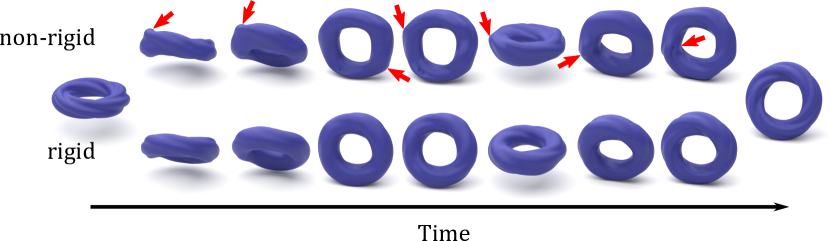
Figure 9: Effect of rigidity regularizer on trajectories of tori. The top row is computed with default parameters, while the bottom row is computed with additional regularization $\lambda_{\text{acc}}=\lambda_{\text{rig}}=10^{-1}$. Red arrows point out several locations where extra deformation occurs without rigidity regularization. Using these regularizers results in less wobbling along the trajectory.

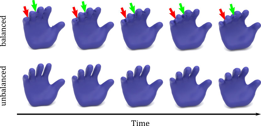
Figure 10: Effect of balanced v.s. unbalanced Wasserstein barycenter interpolation on intermediate frames of a hand closing animation. Volume of fingers is not carefully tuned in keyframes, resulting in balanced OT necessarily transporting mass between fingers during the animation. This is pointed out in the balanced interpolation, where red and green arrows track lumps of mass moving between fingers. Using unbalanced Wasserstein barycenters instead alleviates the mass splitting, and fingers are clearly separated throughout the animation.

Volumetric Results.

In Figure 9, we show various frames of an animation of a spinning ring with and without regularizers. In the first row we only use the default regularizer $\lambda_{\text{jerk}}=10^{-1}$. Since the loss does not care about rigidity, the resulting trajectory develops bulges indicated by the red arrows. In the second row we additionally regularize with $\lambda_{\text{acc}}=\lambda_{\text{rig}}=10^{-1}$ to produce a much tamer trajectory.

In Figure 10, we show the effect of unbalanced Wasserstein barycenter interpolation on interpolations of the same keyframes and the same neural ODE. The only difference is in the Wasserstein barycenter interpolation step Equation 20, where the first row is computed with default parameter $\tau=\infty$, and the second row with $\tau=0.05$. Recall from subsection 3.3 that $\tau$ represents how much distance a transport plan is willing to move mass before giving up on constraints of the classical OT problem. Since fingers of the hand animation keyframes have different volumes, animations generated with $\tau=\infty$ necessarily transfer mass between fingers. This is tracked by the red and green arrows indicating mass moving between fingers. When we use unbalanced Wasserstein barycenters, the mass balancing between fingers is alleviated resulting in much sharper distinctions between each individual finger.

Wassersplines for Neural Vector Field–Controlled Animation summarizes application of our method to generate 3D animations. In the first row, we build in-between frames for an animation from an open hand, to a partially closed hand, and finally to a cat. This animation is regularized with $\lambda_{\text{acc}}=\lambda_{\text{rig}}=10^{-1}$. We use unbalanced Wasserstein barycenter interpolation with $\tau=.05$ for in-between frames from the open hand to the partially closed hand. Due to the increased complexity of computing unbalanced Wasserstein barycenters, we reserve the unbalanced case for only where we explicitly want to alleviate mass splitting and otherwise default to balanced barycenters. In the second row, we interpolate from a sphere to a cow to a torus with all default parameters. The change in topology is handled seamlessly. In the last row, we interpolate through five keyframes of rings at different angles. The first, third, and fifth keyframes are rings with detailed helical patterns carved into them, while the second and fourth keyframes are normal tori. We regularize this animation with $\lambda_{\text{acc}}=\lambda_{\text{rig}}=10^{-1}$ to produce a smooth trajectory.

7 Discussion and Conclusion

Unstructured animations appear in various forms of media ranging from hand-drawn to video games and film. These animations share a fluid morphing capability that is mesmerizing to watch but challenging to construct. Our work identifies unstructured animation as a density interpolation problem and builds automatic solutions through the machinery of optimal transport, neural ODEs, and PDE-based regularizers for intuitive and varied control.

Future work might consider discontinuous parameterizations of the velocity field. Depending on the context, spatially discontinuous trajectories may be desirable, but integration of a smooth velocity field will always produce a diffeomorphism. Discontinuous velocity fields provide added flexibility, but also pose challenges to gradient based optimization and ODE integration. A natural regularizer in this setting is vectorial total variation [GC10], which measures vector field smoothness but does not diverge near discontinuities.

Another avenue for further exploration might be to treat the fitting loss as a constraint. If the fitting loss can reach exactly 0, Wasserstein barycenter interpolation would no longer be necessary. The final rendering quality of our animations depend in part on the number of samples used to build the trajectory. Since the Wasserstein barycenter interpolation is computed independently per in-between frame and scales in expense with the number of points, it would be ideal to skip computing barycenters altogether.

Mesh- and rig-based animation are approachable for beginners through the abundance of accessible tools and tutorials. Unstructured animation is the opposite: Almost no documented computational tools exist enabling its design. This paper represents a step toward bridging the gap between rig-based animation and unstructured animation. We hope that the graphics community will discover more exciting approaches toward unstructured animation to further improve its ease of construction and accessibility.

References

- [ACB17] Martin Arjovsky, Soumith Chintala and Léon Bottou “Wasserstein generative adversarial networks” In International conference on machine learning, 2017, pp. 214–223 PMLR
- [BB00] Jean-David Benamou and Yann Brenier “A computational fluid mechanics solution to the Monge-Kantorovich mass transfer problem” In Numerische Mathematik 84.3 Springer, 2000, pp. 375–393
- [BBRF14] Mark Browning, Connelly Barnes, Samantha Ritter and Adam Finkelstein “Stylized keyframe animation of fluid simulations” In Proceedings of the Workshop on Non-Photorealistic Animation and Rendering, 2014, pp. 63–70
- [BBSG10] Mirela Ben-Chen, Adrian Butscher, Justin Solomon and Leonidas Guibas “On discrete killing vector fields and patterns on surfaces” In Computer Graphics Forum 29.5, 2010, pp. 1701–1711 Wiley Online Library
- [BGV19] Jean-David Benamou, Thomas O Gallouët and François-Xavier Vialard “Second-order models for optimal transport and cubic splines on the Wasserstein space” In Foundations of Computational Mathematics 19.5 Springer, 2019, pp. 1113–1143
- [BVPH11] Nicolas Bonneel, Michiel Van De Panne, Sylvain Paris and Wolfgang Heidrich “Displacement interpolation using Lagrangian mass transport” In Proceedings of the 2011 SIGGRAPH Asia Conference, 2011, pp. 1–12
- [CCG18] Yongxin Chen, Giovanni Conforti and Tryphon T Georgiou “Measure-valued spline curves: An optimal transport viewpoint” In SIAM Journal on Mathematical Analysis 50.6 SIAM, 2018, pp. 5947–5968
- [CCL*21] Sinho Chewi et al. “Fast and smooth interpolation on Wasserstein space” In International Conference on Artificial Intelligence and Statistics, 2021, pp. 3061–3069 PMLR
- [CRBD18] RTQ Chen, Y Rubanova, J Bettencourt and D Duvenaud “Neural Ordinary Differential Equations (NeurIPS)”, 2018
- [Cut13] Marco Cuturi “Sinkhorn distances: Lightspeed computation of optimal transport” In Advances in neural information processing systems 26, 2013, pp. 2292–2300
- [ELC19] Marvin Eisenberger, Zorah Lähner and Daniel Cremers “Divergence-Free Shape Correspondence by Deformation” In Computer Graphics Forum 38, 2019
- [FCG*21] Rémi Flamary et al. “POT: Python Optimal Transport” In Journal of Machine Learning Research 22.78, 2021, pp. 1–8 URL: http://jmlr.org/papers/v22/20-451.html
- [FCVP17] Jean Feydy, Benjamin Charlier, François-Xavier Vialard and Gabriel Peyré “Optimal transport for diffeomorphic registration” In International Conference on Medical Image Computing and Computer-Assisted Intervention, 2017, pp. 291–299 Springer
- [Fey20] Jean Feydy “Geometric data analysis, beyond convolutions”, 2020
- [FJNO20] Chris Finlay, Jörn-Henrik Jacobsen, Levon Nurbekyan and Adam Oberman “How to train your neural ODE: the world of Jacobian and kinetic regularization” In International Conference on Machine Learning, 2020, pp. 3154–3164 PMLR
- [FSV*19] Jean Feydy et al. “Interpolating between optimal transport and MMD using Sinkhorn divergences” In The 22nd International Conference on Artificial Intelligence and Statistics, 2019, pp. 2681–2690 PMLR
- [GC10] Bastian Goldluecke and Daniel Cremers “An approach to vectorial total variation based on geometric measure theory” In 2010 IEEE Computer Society Conference on Computer Vision and Pattern Recognition, 2010, pp. 327–333 IEEE
- [GCB*18] Will Grathwohl et al. “FFJORD: Free-Form Continuous Dynamics for Scalable Reversible Generative Models” In International Conference on Learning Representations, 2018
- [GPC18] Aude Genevay, Gabriel Peyré and Marco Cuturi “Learning generative models with sinkhorn divergences” In International Conference on Artificial Intelligence and Statistics, 2018, pp. 1608–1617 PMLR
- [HMP15] Romain Hug, Emmanuel Maitre and Nicolas Papadakis “Multi-physics optimal transportation and image interpolation” In ESAIM: Mathematical Modelling and Numerical Analysis 49.6 EDP Sciences, 2015, pp. 1671–1692
- [HPG*21] Amir Hertz et al. “SAPE: Spatially-adaptive progressive encoding for neural optimization” In Advances in Neural Information Processing Systems 34, 2021
- [KA08] Michael Kass and John Anderson “Animating oscillatory motion with overlap: wiggly splines” In ACM Transactions on Graphics (TOG) 27.3 ACM New York, NY, USA, 2008, pp. 1–8
- [Kan06] Leonid V Kantorovich “On the translocation of masses” In Journal of mathematical sciences 133.4 Kluwer Academic Publishers-Consultants Bureau, 2006, pp. 1381–1382
- [KB14] Diederik Kingma and Jimmy Ba “Adam: A Method for Stochastic Optimization” In International Conference on Learning Representations, 2014
- [KBJD20] Jacob Kelly, Jesse Bettencourt, Matthew J Johnson and David K Duvenaud “Learning Differential Equations that are Easy to Solve” In Advances in Neural Information Processing Systems 33 Curran Associates, Inc., 2020, pp. 4370–4380 URL: https://proceedings.neurips.cc/paper/2020/file/2e255d2d6bf9bb33030246d31f1a79ca-Paper.pdf
- [Las87] John Lasseter “Principles of traditional animation applied to 3D computer animation” In Proceedings of the 14th annual conference on Computer graphics and interactive techniques, 1987, pp. 35–44
- [Lav21] Hugo Lavenant “Unconditional convergence for discretizations of dynamical optimal transport” In Mathematics of Computation 90.328, 2021, pp. 739–786
- [LCCS18] Hugo Lavenant, Sebastian Claici, Edward Chien and Justin Solomon “Dynamical optimal transport on discrete surfaces” In ACM Transactions on Graphics (TOG) 37.6 ACM New York, NY, USA, 2018, pp. 1–16
- [LZKS21] Hugo Lavenant, Stephen Zhang, Young-Heon Kim and Geoffrey Schiebinger “Towards a mathematical theory of trajectory inference” In arXiv preprint arXiv:2102.09204, 2021
- [PC*19] Gabriel Peyré and Marco Cuturi “Computational optimal transport: With applications to data science” In Foundations and Trends® in Machine Learning 11.5-6 Now Publishers, Inc., 2019, pp. 355–607
- [PM17] Zherong Pan and Dinesh Manocha “Efficient solver for spacetime control of smoke” In ACM Transactions on Graphics (TOG) 36.4 ACM New York, NY, USA, 2017, pp. 1
- [PMY*20] Michael Poli et al. “Hypersolvers: Toward Fast Continuous-Depth Models” In Advances in Neural Information Processing Systems 33, 2020
- [PNR*21] George Papamakarios et al. “Normalizing Flows for Probabilistic Modeling and Inference” In Journal of Machine Learning Research 22.57, 2021, pp. 1–64 URL: http://jmlr.org/papers/v22/19-1028.html
- [PPO14] Nicolas Papadakis, Gabriel Peyré and Edouard Oudet “Optimal transport with proximal splitting” In SIAM Journal on Imaging Sciences 7.1 SIAM, 2014, pp. 212–238
- [Ric21] Jacob Benjamin Rice “Weaving The Druun’s Webbing” In ACM SIGGRAPH 2021 Talks, 2021, pp. 1–2
- [RM15] Danilo Rezende and Shakir Mohamed “Variational inference with normalizing flows” In International conference on machine learning, 2015, pp. 1530–1538 PMLR
- [San15] Filippo Santambrogio “Optimal transport for applied mathematicians” In Birkäuser, NY 55.58-63 Springer, 2015, pp. 94
- [SDP*15] Justin Solomon et al. “Convolutional wasserstein distances” In ACM Transactions on Graphics 34.4 Association for Computing Machinery, 2015, pp. 66:1–66:11 DOI: 10.1145/2766963
- [Sol18] Justin Solomon “Optimal transport on discrete domains” In AMS Short Course on Discrete Differential Geometry, 2018
- [SST*19] Geoffrey Schiebinger et al. “Optimal-transport analysis of single-cell gene expression identifies developmental trajectories in reprogramming” In Cell 176.4 Elsevier, 2019, pp. 928–943
- [TCCS21] Jingwei Tang, Vinicius C., Guillaume Cordonnier and Barbara Solenthaler “Honey, I Shrunk the Domain: Frequency-aware Force Field Reduction for Efficient Fluids Optimization” In Computer Graphics Forum 40.2, 2021, pp. 339–353 Wiley Online Library
- [THW*20] Alexander Tong et al. “Trajectorynet: A dynamic optimal transport network for modeling cellular dynamics” In International Conference on Machine Learning, 2020, pp. 9526–9536 PMLR
- [TJT95] Frank Thomas, Ollie Johnston and Frank Thomas “The illusion of life: Disney animation” Hyperion New York, 1995
- [TMPS03] Adrien Treuille, Antoine McNamara, Zoran Popović and Jos Stam “Keyframe control of smoke simulations” In ACM SIGGRAPH 2003 Papers, 2003, pp. 716–723
- [TSM*20] Matthew Tancik et al. “Fourier Features Let Networks Learn High Frequency Functions in Low Dimensional Domains” In Advances in Neural Information Processing Systems 33 Curran Associates, Inc., 2020, pp. 7537–7547 URL: https://proceedings.neurips.cc/paper/2020/file/55053683268957697aa39fba6f231c68-Paper.pdf
- [WZ89] Ronald J Williams and David Zipser “A learning algorithm for continually running fully recurrent neural networks” In Neural computation 1.2 MIT Press One Rogers Street, Cambridge, MA 02142-1209, USA journals-info …, 1989, pp. 270–280