POLYLLA: Polygonal meshing algorithm based on terminal-edge regions

Abstract

This paper presents an algorithm to generate a new kind of polygonal mesh obtained from triangulations. Each polygon is built from a terminal-edge region surrounded by edges that are not the longest-edge of any of the two triangles that share them. The algorithm is termed Polylla and is divided into three phases. The first phase consists of labeling each edge of the input triangulation according to its size; the second phase builds polygons (simple or not) from terminal-edges regions using the label system; and the third phase transforms each non simple polygon into simple ones. The final mesh contains polygons with convex and non convex shape. Since Voronoi based meshes are currently the most used polygonal meshes, we compare some geometric properties of our meshes against constrained Voronoi meshes. Several experiments were run to compare the shape and size of polygons, the number of final mesh points and polygons. For the same input, Polylla meshes contain less polygons than Voronoi meshes and the algorithm is simpler and faster than the algorithm to generate constrained Voronoi meshes. Finally, we have validated Polylla meshes by solving the Laplace equation on an L-shaped domain using the Virtual Element Method (VEM). We show that the numerical performance of the VEM using Polylla meshes and Voronoi meshes is similar.

Article Highlights

• A simple and automatic tool to generate polygonal meshes composed of convex or/and non-convex polygons.

• The polygonal meshes are composed of less polygons and points than constrained Voronoi meshes for the same input

• A new kind of polygonal meshes for the virtual element method.

1 Introduction

Meshes composed of triangles and quadrilaterals are common in simulations using the Finite Element Method (FEM). One of the main requirements is that polygons (elements) need to obey specific quality criteria such as angles not too large or small, or reasonable aspect ratio and area, among others. To fulfill these criteria, sometimes the insertion of a large number of points and elements is required in order to properly model a domain, increasing the time needed to make a simulation. New methods such as the Virtual Element Method (VEM) Basisprinciples ; Brezzi2015 can use any polygon as basic cell. Our main research interest is to explore how far the VEM can handle non-convex and convex polygons and still be able to compute accurate simulation results. Our goal is to build a new tool that allows the VEM community Wriggers2019 to model and simulate more complex problems than before, both in 2D and 3D.

In this context, the VEM presents an opportunity to explore new kind of polygonal meshes and new algorithms to generate them. Our main research questions are: Can terminal-edge regions  be adapted to be used as good basic cells for polygonal numerical methods such as the VEM? Do this kind of meshes require less polygons to model the same problem than polygonal meshes based on the Voronoi diagram? Our hypotheses are: (i) Terminal-edge regions can be transformed into simple polygons and used as basic cells, (ii) the domain geometry can be fitted using less elements than constrained Voronoi meshes, (iii) this kind of polygonal meshes can be used with the VEM.

In this paper, we propose an algorithm to generate meshes that adapt to a geometric domain specified through Planar line straight graph (PLSG) using polygons of any shape, and respecting the point distribution given as input. The algorithm reads as input a triangulation and uses the concept of terminal-edge region as basis to build polygons. Terminal-edge regions can generate non-simple polygons, so we also propose an algorithm to divide them into simple ones. We run several experiments to show properties of these polygons and compare the generated meshes against constrained Voronoi meshes. Moreover, we validate the polygonal meshes over a classical problem to show that these meshes can be used to solve problems with the VEM. As an example, Fig. 1 shows a polygonal mesh generated with the algorithm proposed in this paper.

Figure 1: Polygonal mesh of a Chilean moth (Polilla Venusta) composed of 513 polygons, 1351 vertices and 2455 edges. The original PLSG contains 616 points and segments. A conforming Delaunay triangulation with maximum edge size of 160 was generated using Pygalmesh Schlomer_pygalmesh_Python_interface . The resulting triangulation contains 1351 vertices (the same of the output), 2083 triangles and 3432 edges.

Any triangulation can be used as input but through this paper the polygonal meshes are generated from a Delaunay triangulation. It is known that Delaunay triangulations are the ones that maximize the smallest angle among all the triangulations of a point set. Since the proposed algorithm does not divide any input triangle, the smallest angle of the triangulation is a lower bound for the minimum interior angle of the polygonal mesh.

The main contributions of this paper are:

• A simple and automatic tool to generate polygonal meshes composed of convex or/and non-convex polygons, fitting exactly the input domain and respecting the initial point distribution.

• A new kind of polygonal meshes composed of less polygons and points than constrained Voronoi meshes for the same input.

• The algorithm benefits from robust tools such as Detri2d or Triangle to generate the initial constrained Delaunay triangulation in similar way some constrained Voronoi meshing algorithms do. Voronoi meshing algorithms require to compute new points (Voronoi points), cut non-bounded Voronoi regions to fit the domain and insert new points at the domain boundary to create the constrained Voronoi mesh. So the proposed algorithm is faster than the algorithm to generate constrained Voronoi meshes.

This paper is organized as follows: Section 2 presents and discusses the-state-of-art; Section 3 introduces the basic concepts that explains the algorithm; Section 4 describes the main steps of the proposed algorithm and the used data structure; in Section 5 we analyse some geometric features of the generated meshes and gives a comparison against the constrained Voronoi meshes; Section 6 shows a preliminary assessment of the meshes in the Virtual Element Method (VEM) and Section 7 presents our conclusions and ongoing work.

2 Related work

Mesh generation refers to the methods used to discretize a geometric domain into smaller elements without overlap. Those methods has been widely studied due to their importance in science and engineering. Meshes are used in geographic information systems PrinciplesGIS , computer vision JOHNSON1998261 and numerical methods HOLE198827 , among other applications. Common methods used to generate unstructured polygon meshes are the Delaunay methods cheng2013delaunay , Voronoi diagram methods yan:hal-00647979 ; 2dcentroidalvoro ; PolyMesher2012 , advancing front method lohner1996progress ; Schberl1997NETGENAA , quadtree based methods BERN1994384 ; bommes2013quad and hybrids methods owen1999q ; ito2002unstructured , among others. In general, meshing algorithms can be classified into two groups owen1998survey ; johnen2016indirect : (i) direct algorithms: meshes are generated from the input geometry, and (ii) indirect algorithms: meshes are generated starting from an input mesh, typically an initial triangle mesh. Indirect methods is a common approach to generate quadrilateral meshes by mixing triangles of an initial triangulation  LeetreetoQuad ; BlossonQuad ; Merhof2007Aniso-5662 . The advantage of using indirect methods is that currently triangular meshes are easy to generate because several robust open source and free tools triangle2d ; Detri2 ; qhull ; cgal:y-t2-21b are available. Polylla mesh generation is an indirect method as it is based on mixing triangles from an initial triangulation.

In standard FEM, the most used 2D meshes are triangulations triangle2d ; Detri2 ; chew1 and quadrilateral meshes Canann98 ; Lee20031055 ; Owen98advancingfront . 2D Mixed meshes composed of triangles and quadrilaterals have also been used, but are not so common as the previous ones jaillet2021 . Other numerical methods such as the Voronoi Cell Finite Element Method (VCFEM) ReviewFEM and Polygonal Finite Element method (PFEM)Chi2015PolygonalFE use the constrained Voronoi diagram as the polygonal mesh, where the Voronoi cells are the mesh elements YanWLL10 ; UniformRandomVoronoiMeshes ; SiegerAB10 .

The generalization of finite element methods to include polygons as part of the mesh elements is not recent zbMATH03504364 ; Sukumar2006 ; tabarraei2008extended . Polygonal elements are usually generated by using a quadtree approach and from Voronoi based algorithms. In particular, the vem was introduced in the last decade  Basisprinciples ; Brezzi2015 and since then, several research groups have been developing computational frameworks in order to explore new problems. To mention some applications, the vem has been formulated and applied to solve linear elastic and inelastic solid mechanics problems da2015virtual , in fluid mechanics ErnestoBRinkmanFluid ; ErnestoQuasiNewtwon , in the optimization of a fluid problem through a discrete network benedetto2014virtual , for compressible and incompressible finite deformations Wriggers2017 ; Wriggers2017a and brittle crack propagation HUSSEIN201915 .

VEM has a flexibility in dealing with complex cell shapes that can even be non convex and have an arbitrary number of vertices Aldakheel_2019 . As an example, meshes composed of animal shape polygons were used for crack propagation to show that the vem can deal with non-convex element shapes Wriggers2019 . Similar experiments using the vem in meshes composed of high irregular shapes are described in PARK2019669 ; CHI2017148 .

To our knowledge, no algorithm for the automatic generation of 2D meshes formed by polygons (convex or not) has been published for the vem in arbitrary domains. We recently developed a tool to generate a particular kind of polygonal meshes in the context of modeling the rock packing problem inside a square container PackingJoaquin . The rocks were modeled as convex polygons and the space with general polygons. We ran preliminary simulations using the vem and also experienced that the vem is very robust under irregular polygonal shapes PackingJoaquin .

3 Basic concepts

The proposed polygonal meshing algorithm is based on two concepts: Longest-edge propagation path (Lepp) introduced in Rivara97 and terminal-edge regions defined in Ascom209 ; Ojeda2018ANA . We briefly review these concepts and some related properties in this section.

3.1 Terminal-edge regions

In any triangulation, triangles can be grouped under the Longest-edge propagation path concept defined as follows:

Definition 1.

Longest-edge propagation path  Rivara97 : For any triangle $t_{0}$ in any triangulation $\Omega$, the Lepp($t_{0}$) is the ordered list of all the triangles $t_{0}$, $t_{1}$, $t_{2}$, …, $t_{l-1}$, $t_{l}$, such that $t_{i}$ is the neighbor triangle of $t_{i-1}$ by the longest-edge of $t_{i-1}$, for $i=1,2,\dots,l$. The longest-edge shared by $t_{l-1}$ and $t_{l}$ is a terminal-edge and $t_{l-1}$ and $t_{l}$ are terminal-triangles. As an example, in Fig. 2 the Lepp($t_{0}$) is shown in blue, its terminal edge is shown in red and its terminal triangles labeled as $t_{1}$ and $t_{2}$.

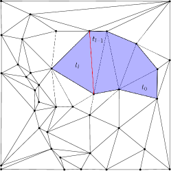
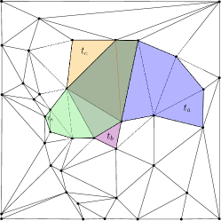
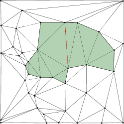
Figure 2: Terminal-edge region. (a) Longest-edge propagation of $t_{0}$ where the red edge is the terminal-edge. (b) Four Lepps: Lepp($t_{a}$), Lepp($t_{b}$), Lepp($t_{c}$) and Lepp($t_{d}$), with the same terminal-edge. (c) Terminal-edge region generated by the union of Lepp($t_{a}$), Lepp($t_{b}$), Lepp($t_{c}$) and Lepp($t_{d}$).

A triangle edge can be classified according to its length inside the two triangles that share it. Therefore, given an edge $e$ and two triangles $t_{1}$, $t_{2}$ that share $e$, we can label $e$ as:

• Terminal-edge Rivara97 : $e$ is the longest-edge of $t_{1}$ and $t_{2}$.

• Frontier-edge Ascom209 : $e$ is neither the longest-edge of $t_{1}$ nor $t_{2}$.

• Internal-edge: $e$ is the longest edge of $t_{1}$ but not of $t_{2}$ or vice-versa.

• Boundary edge: $e$ belongs to one triangle. In the proposed algorithm boundary edges are handled as frontier edges.

It is worth mentioning that edges of equal length can appear. Therefore, in case there are equilateral triangles, each edge is chosen arbitrarily as the longest-, the middle- and smallest-edge. When there are isosceles triangles, something similar is done for equal size edges.

Definition 2.

Terminal-edge region Ascom209 : A terminal-edge region $R$ is a region formed by the union of all triangles $t_{i}$ such that Lepp($t_{i}$) has the same terminal-edge. In case the terminal-edge region is partially delimited by boundary edges the region will be called boundary terminal-edge region. Fig. 2(c) shows the terminal-edge region formed by the union of Lepp($t_{a}$), Lepp($t_{b}$), Lepp($t_{c}$) and Lepp($t_{d}$).

We have already used the concept of terminal-edge region for finding polygonal voids (holes) inside a point set HerviasHCF13 ; Ascom209 and proven some geometric properties. In order to facilitate understanding of the algorithm we are recalling the most important here:

• Terminal-edge regions are surrounded by frontier-edges Ascom209 .

• Terminal-edge regions cover the whole domain without overlapping Ascom209 ; Ojeda2018ANA .

• Terminal-edge-regions might include frontier-edges in their interior. We have called this kind of frontier-edge a barrier-edge Ascom209 ; Ojeda2018ANA .

Let us use Fig. 3 to illustrate an example of a partition generated by terminal-edge regions. Fig. 3 shows an input point set; Fig. 3 shows the Delaunay triangulation of this point set where terminal-edges are drawn using red dashed lines, internal-edges using black dashed lines and frontier-edges using solid lines. Fig. 3 shows the polygons defined by terminal-edge regions using a different color, where each polygon is delimited by frontier edges. It can be noticed that the green polygon is a non-simple polygon because it includes a barrier-edge. For simplicity, in the case $e$ is a domain boundary edge, $e$ will be considered a frontier-edge too (see the edges belonging to the square in Figs. 3 and 3).

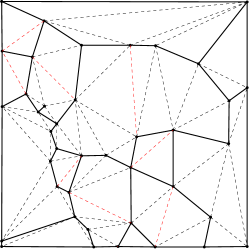
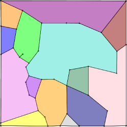
Figure 3: (a) Initial random point set. (b) Delaunay triangulation: Solid lines are frontier-edges, dashed black lines are internal-edges and red dashed lines are terminal-edges. (c) Polygon partition from terminal-edge regions.

3.2 Terminal-edge regions as polygons

As we have said in the previous section, terminal-edge regions generate a polygon partition of the domain without overlapping. Depending on the point distribution, polygons can be simple or non-simple polygons. Non-simple polygons appear when terminal-edge regions include barrier-edges. As observed in Fig. 3, the domain was tessellated into 14 polygons where only the green region is represented by a non-simple polygon because it includes one barrier-edge.

In order to build a conforming polygon tessellation from the partition generated by the terminal-edge regions, non-simple polygons must be divided into simple polygons. That requires the integration of barrier-edges as part of the boundary of new simple polygons. Since this requirement is part of the meshing algorithm we are proposing in Section 4, beforehand, we need to introduce some definitions and prove some properties that will sustain the correctness of the algorithm.

Definition 3.

Barrier-edge tip: A barrier-edge tip in a terminal-edge region $R$ is a barrier-edge endpoint shared by no other barrier-edge/frontier-edge.

Fig. 4 includes two polygons with barrier-edges; the barrier-edge tips are shown in green. Fig. 4 shows a case of a polygon with one barrier-edge tip and Fig. 4 a case with two barrier-edge tips. We have observed that each point of the input data is an endpoint of a frontier-edge or barrier-edge. This means that terminal-edge regions have none isolated interior points. Theorem 1 demonstrates this property.

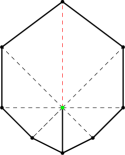
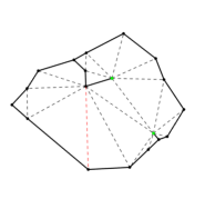
Figure 4: Examples of non-simple polygons. Black lines are frontier-edges, dashed black lines are internal-edges and red edges are terminal-edges. (a) One barrier-edge and one tip (b) Four barrier-edges and two tips tip

Theorem 1.

Let $\Omega$ be a triangulation with the set of vertices $V$ in general position. Then, each vertex $v$ is an end-point of at least one of the frontier- or barrier-edges, i.e. there is no isolated interior points (vertices incident only to internal-edges).

Proof: : Let $v$ be a vertex associated to the terminal-edge region $R$ generated by the terminal-edge $e$ and $T$ the set of the triangles that share $v$. By contradiction, let us assume that $v$ is an interior point of $R$ as shown in Fig. 5. Since the triangles in $T$ are part of $R$, they must share their longest-edge around $v$. Given that $T$ is finite, there should exist a triangle $t_{0}$ (see Fig. 5) that shares their longest-edge with two triangles of $R$ in order to maintain $v$ interior point in $R$. This is not possible because a triangle has just one edge labeled as its longest-edge. This contradicts our assumption, so $v$ has to be an endpoint of at least one frontier- or barrier-edge in $R$. Since triangles in $\Omega$ are distributed into terminal-edge regions without overlap Ojeda2018ANA , isolated points can not exist.

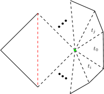
Figure 5: The vertex in green is an interior point.

It is worth mentioning Theorem 1 guarantees that the initial points used to represent the geometric domain and the ones inside the domain to fulfill point density requirements are vertices delimiting one or more polygons. Moreover, each internal-edge is a diagonal of one polygon. Therefore, interior-edges that contain barrier-edge tips as endpoints can be used to split a non-simple polygon into simple polygons.

Note that if the input points are not in general position, a region without a terminal-edge might appear. This degenerate region $R$ occur when the algorithm labels all edges that share a vertex $v$ as internal-edges. This case might happen if all triangles in $R$ are equilateral and the algorithm labels each edge $e$ sharing $v$ as the longest-edge in only one of the triangles that share $e$. Then all edges that share $v$ are internal-edges. This rare kind of case can be solved by assigning one edge with $v$ as endpoint as longest-edge in the two triangles that share it. In this way, $R$ is now a terminal-edge region.

4 The algorithm

In this section, we describe the main steps of the proposed algorithm, its computational cost and the data structure used for its implementation. The algorithm receives an initial triangulation as input, that can be generated by any known triangulator. The triangulation can be Delaunay or not, but we are using Delaunay triangulations because, several polygons of the mesh keep some angles of the triangles of the input triangulation. Since a Delaunay triangulation maximizes the minimum angle over all the possible triangulations for a point set, this angle will be a lower bound for the minimum angle of the generated polygonal mesh.

There are several correct and robust triangulators such as Detri2 Detri2 and Triangle triangle2d available for free. We are using Detri2 Detri2 to generate the constrained Delaunay triangulation needed as initial mesh. The whole process applied to the initial triangulation is divided in next three phases:

1. Label phase: Each edge is labeled as longest-, terminal- or frontier-edges to build terminal-edge regions. The algorithm also labels one triangle in each terminal-edge region as seed triangle used in the next phase to build each polygon.

2. Traversal phase: Generation of polygons from seed triangles. In this phase the frontier-edge vertices of a terminal-edge region are stored in counter-clock-wise (ccw) order to build a polygon. Non-simple polygons generated in this phase are sent to the reparation phase.

3. Reparation phase: Polygons with barrier-edges are partitioned into simple polygons.

4.1 Data structures

In this subsection we describe the data structures used in our implementation. We have decided to use an indexed data structure with adjacencies as described in MeshDatastructSurvey . The purpose of the following representation is to have an easy and compact way to travel through all the faces of the triangulation and, in an implicit way, by using a special order in the representation, to access their edges and neighbor triangles in ccw.

The triangulation is represented using three one-dimensional arrays for the vertices, triangles and neighbor triangles, respectively. Vertices are stored in pairs $(x,y)$, where each two consecutive elements of the Vertex array are the coordinates $x$ and $y$ of a point. The Triangle array is a set of indices to the Vertex array. Each 3 consecutive values is a triangle. Since the algorithm needs to know the neighbor through each triangle edge, the Neighbor array stores the three indices of the neighbor triangles of triangle $i$ at the locations $3i+0$, $3i+1$, $3i+2$.

To facilitate the implementation of the algorithm, vertex indices in the Triangle array are ordered in such a manner that is easy to find out which is the neighbor triangle through each triangle edge. Fig. 6(a) illustrates the connections of each array element. The first two point indices $3i+0$, $3i+1$ in the Triangle array is an edge of triangle $i$ and this edge is shared with the triangle stored in the position $3i+2$ of the Neighbor array; the triangle edge defined by $3i+1$, $3i+2$ in the Triangle array is shared with the triangle stored in $3i+0$ in the Neighbor array and the triangle edge $3i+2$, $3i+0$ in the Triangle array with the triangle stored at $3i+1$ in Neighbor array. Triangle edges are stored implicitly: the green edge in Fig. 6(b) corresponds to the first one, the red edge is the second one and the blue the third one. These neighborhood relations can currently be generated as output by several tools such as Qhull qhull , Triangle triangle2d and Detri2qt Detri2 .

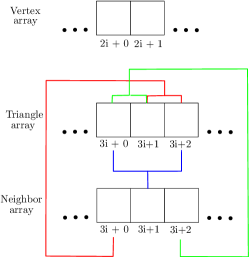
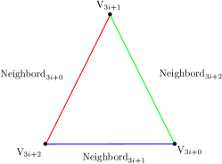
Figure 6: Data structure: (a) Relation between the vertex indices in the Triangle array and the triangle indices in the Neighbor array. (b) Triangle information stored in the data structure shown in (a) .

The final mesh composed of simple polygons is also stored in one array, where each polygon includes first its number of vertices and then the vertex indices in ccw as shown in Fig. 7.

Data structures to store additional information needed only in one of the steps of the algorithm are mentioned in the respective subsection. It is worth mentioning here the representation of non-simple polygons since this information is used in two phases. Fig. 8 shows an example of a polygon with two barrier edge tips. This kind of polygon is stored in an index array in the same way as a simple polygon in order ccw, and it is recognized as non-simple because there are repeated vertex indices. The same occurs with the seed list $L$, which is initialized in the Label phase with one triangle index per each terminal-edge region, and used in the Traversal phase to build polygons.

Figure 7: Mesh array with three polygons.

Figure 8: Representation of a non-simple polygon as a set of vertex indices in ccw. Sequences $3-4-3$ and $3-5-3$ indicate the existence of barrier-edge tips.

4.2 Label Phase

The goal of the Label phase is to find frontier-edges, terminal-edges and seed triangles to build polygons in the next phase. The pseudo-code of this process is shown in Algorithm 1. The algorithm first cycles over each triangle of the initial triangulation (line 3) to compute which edge is the longest-edge and stores this edge index (one per each triangle) in a temporal array of size equal to the number of triangles; in the case of equilateral and isosceles triangles, the algorithm assigns randomly a size order to the equal length edges to avoid having a triangle that belongs to two terminal-edge regions at the same time.

Afterward, the algorithm does a second iteration over the edges (line 6). In case an edge $e$ is not the longest-edge of any of the two triangles that share it (line 8), $e$ is labeled as a frontier-edge. In case $e$ is a terminal-edge (line 11), the algorithm stores the smallest index of the triangles that share it in the Seed list $L$. In the case of a boundary terminal-edge, the index of the unique triangle is stored.

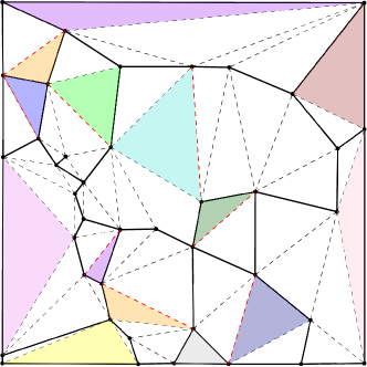
Figure 9: Label phase: (a) Input Delaunay triangulation. (b) Solid lines are the frontier-edges, dashed lines are the internal-edges and colorful triangles are seed triangles.

The final result of this step is shown in Fig. 9(b). The colorful triangles are the seeds used in the next phase to generate the polygons. It can also be observed that terminal-edge regions are delimited by frontier-edges.

Algorithm 1 Label phase

1:Initial Triangulation $\Omega$

2:Labeled edges and seed triangles of $\Omega$

3:for all triangle $t_{i}$ in $\Omega$ do

4:     Label the longest-edge of $t_{i}$

5:end for

6:for all edge $e_{i}$ in $\Omega$ do

7:     Be $t_{1}$ and $t_{2}$ triangles that share $e_{i}$

8:     if $e_{i}$ neither the longest-edge of $t_{1}$ nor $t_{2}$ or $e_{i}$ is border-edge then

9:         Label $e$ as frontier-edge

10:     end if

11:     if $e_{i}$ is terminal-edge or border terminal-edge then

12:         Choose one triangle sharing $e_{i}$ and store its index in the Seed list $L$

13:     end if

14:end for

4.3 Traversal Phase

In this phase, polygons are built and represented as a closed polyline as shown in Fig. 8. The main idea behind this phase is to travel through neighbor triangles, neighbors by internal-edges inside a terminal-edge region and save their frontier-edges as edges of the new polygon $P$ in ccw. For this reason, the algorithm uses each triangle $t$ inserted in the Seed list $L$ as the starting triangle to build each polygon. The pseudo-code of this phase is shown in Algorithm 2.

From line 3 until line 15, the algorithm gets the first triangle $t$ from the Seed list and initializes the variables according to the number of frontier-edges that $t$ has. In case $t$ has 3 frontier-edge edges, $t$ is stored in the polygon $P$ as a whole polygon. In case $t$ has less than $3$ frontier-edges, their endpoints are saved as the first points of $P$ in ccw. In addition, the first vertex of $P$ and $t$ are saved in $v_{init}$ and $t_{init}$, respectively, to check when the polygon boundary is ready. It is also necessary to store the last added vertex in $P$ in $v_{end}$ to look for the e endpoint to be added. In case $t$ has no frontier-edge (Line 12), the algorithm saves any vertex of $t$ as $v_{init}$ and $v_{end}$, and $t$ in $t_{init}$. In the end, all vertices of $t$ will be part of polygon boundary; then it does not matter which one is taken as the initial point. After the initialization, the algorithm travels to the next internal-edge neighboring triangle $t^{\prime}$ that shares $v_{end}$ with $t$. Three cases for $t^{\prime}$ must be considered:

1. Line 17: The triangle $t^{\prime}$ has just one frontier-edge $e$ and this edge contains $v_{end}$. Then $e$ is stored in $P$ and $v_{end}$ is updated with the other $e$ endpoint. The next triangle $t^{\prime}$ is the non-visited internal-edge neighbor triangle that contains the new $v_{end}$.

2. Line 21: The triangle $t^{\prime}$ is an ear triangle (a triangle with 2 frontier-edges). In this case, both edges are stored in ccw in $P$ and $v_{end}$ is updated with last stored endpoint. The previously visited triangle is the new $t^{\prime}$ because the other two triangles are neighbor by frontier-edges (i.e., they belong to other terminal-edge regions).

3. Line 25: The triangle $t^{\prime}$ has no frontier-edge. $t^{\prime}$ shares an internal-edge with the last visited triangle and with the other two neighbor triangles that can be visited. Just one of these two triangles contains the endpoint $v_{end}$ as vertex, so that triangle is the new $t^{\prime}$.

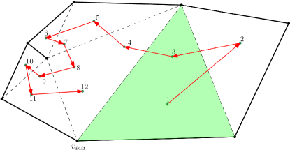
Figure 10: Traversal phase. The green triangle is the seed triangle of this terminal-edge region. The labels indicate in which order each triangle was visited.

Algorithm 2 Polygon construction

1:Seed triangle $t$ of a terminal-edge region

2:Arbitrary shape polygon

3:Polygon $\leftarrow$ $\emptyset$

4:if  $t$ has $3$ frontier-edges $e_{1}$, $e_{2}$ and $e_{3}$ then

5:     return Polygon $\leftarrow$ $e_{1}\cup e_{2}\cup e_{3}$

6:else if  $t$ has $2$ frontier-edges $e_{1}$ and $e_{2}$ then

7:     $v_{init}\leftarrow e_{1}.v_{first}$, $v_{end}\leftarrow e_{2}.v_{second}$

8:     Polygon $\leftarrow$ $e_{1}\cup e_{2}$

9:else if  $t$ has $1$ frontier-edge $e_{1}$ then

10:     $v_{init}\leftarrow e_{1}.v_{first}$, $v_{end}\leftarrow e_{1}.v_{second}$

11:     Polygon $\leftarrow$ $e_{1}$

12:else if $t$ has no frontier-edges then

13:     $v_{init},v_{end}\leftarrow t.v_{0}$

14:end if

15:$t^{\prime}\leftarrow$ internal-edge neighbor triangle of $t^{\prime}$ that shares $v_{end}$

16:while $v_{init}\not=v_{end}$ and $t^{\prime}\not=t_{init}$ do

17:     if  $t^{\prime}$ has $2$ frontier-edges $e_{1}$ and $e_{2}$ with $e_{1}$ continuous to $v_{end}$ then

18:         Polygon $\leftarrow$ Polygon $\cup$ $e_{1}\cup e_{2}$

19:         $v_{end}\leftarrow e_{2}.v_{second}$

20:         $t^{\prime}\leftarrow$ last visited triangle

21:     else if $t^{\prime}$ has $1$ frontier-edge $e_{1}$ continuous to $v_{end}$ then

22:         $v_{end}\leftarrow e_{1}.v_{second}$

23:         Polygon $\leftarrow$ Polygon $\cup$ $e_{1}$

24:         $t^{\prime}\leftarrow$ internal-edge neighbor triangle not visited in previous iteration that contains $v_{end}$

25:     else

26:         $t^{\prime}\leftarrow$ internal-edge neighbor triangle in ccw that contains $v_{end}$

27:     end if

28:end while

29:return Polygon $P$

Algorithm 2 is applied to each seed triangle and returns a polygon $P$. Note that triangles with no frontier-edges are visited 3 times, with one frontier-edge two times and with two frontier-edges one time; this is demostrated in Lemma 1. In case $P$ has barrier-edge tips, the algorithm described in Section 4.4 is used to divide it into simple-polygons. A non-simple polygon can be easily detected by just checking the repetition of consecutive vertices in $P$: given three consecutive vertices of $P$, $v_{i}$, $v_{j}$ and $v_{k}$, if $v_{i}$ and $v_{k}$ are equal, then $v_{j}$ is a barrier-edge tip. In case $P$ does not have barrier-edge tips, the polygon is saved as part of the mesh in the Mesh array.

Lemma 1.

Each triangle is visited at most $3$ times during the polygon construction from a terminal-edge region.

Proof: : By construction, the algorithm can only visit triangles through their internal edges. The worst case is when a triangle has 3 internal edges (no frontier-edges); then this triangle is visited once per internal edge, i.e. 3 times. In case of 2-internal edges, the triangle is visited 2 times and in case of 1 internal-edge just 1 time.

4.4 Non-simple polygon reparation

As previously mentioned, some polygons generated in the Traversal phase are non-simple. In this section, we describe an algorithm to divide non-simple polygons into simple-ones by using internal-edges containing barrier-edge tips as one of their end-points. Notice that a simple strategy could just be to remove barrier-edges and keep as polygon boundary only the frontier-edges. However, this approach would require to delete barrier-edge endpoints, which are vertices defined/inserted in the initial triangulation by the user/triangulation tool. We assume that all points are important. That is why, we propose a method to repair non-simple polygons without removing initial vertices.

The reparation process works similarly to the Label and Traversal phases but inside a non-simple polygon $P$. In short, the algorithm labels so many internal edges as frontier-edges until all barrier-edge tips are part of a polygon boundary and stores one seed triangle per each new polygon in a new Seed list $L_{p}$. After, those triangles are used as seed to generate the new polygons with the Algorithm 2. The internal-edges chosen to be new frontier edges are the ones that contribute to generate polygons of similar size.

The reparation algorithm is shown in Algorithm 3. For each barrier-edge tip $b_{i}$ in a polygon $P$ (line 6), the algorithm computes first $deg(b_{i})$, which is the number of incident internal-edges to $b_{i}$ inside the terminal-edge region. To facilitate this calculation the algorithm uses an auxiliary array that associates to each vertex a triangle. If $deg(b_{i})$ is odd then the algorithm labels the middle edge as frontier-edge; otherwise, the algorithm chooses any of the two middle edges as a new frontier-edge. In both cases, the two triangles that share the new frontier-edge are saved in the seed list $L_{p}$. From line 12 to line  16, each new simple polygon is built. A Bit array $A$, of size equal to the number of triangles of the input triangulation is used to avoid the generation of the same polygon more than once. The insertion of one or more seed triangles of the same new polygon in the seed list $L_{p}$ occurs when a terminal-edge region contains more than one barrier-edge tip. Each seed triangle stored in $L_{p}$ is set to 1 in $A$; the others are 0. When a polygon is built, each used triangle is set to $0$ in $A$. Fig. 11 shows an example of a non-simple polygon with three barrier-edge tips (vertices in green color). Fig. 11 shows the internal-edges converted in new frontier-edges to delimit the new simple polygons and the six seed triangles stored in $L_{p}$. Fig. 11 shows the four new polygons after the split and the seed triangles used to generate them.

It is worth mentioning that the number of polygons generated after the split is at most $(\lvert B\rvert+1)$, with $\lvert B\rvert$ the number of barrier-edge tips in a polygon $P$.

Lemma 2.

Let $\Omega$ be the input triangulation and $B$ the set of barrier edge tips in the polygon $P$. In the computation of $deg(b_{i})$, $\forall b_{i},b_{i}\in B$, each triangle $t$ inside the terminal-edge region that generated $P$ can be visited at most 3 times.

Proof: : By construction if a triangle $t$ is not incident to a barrier-edge tip $b_{i}$, Algorithm 3 does not visit $t$ during the computation of $deg(b_{i})$. If $t$ contains as vertex one, two or three barrier-edge tips, then $t$ is visited one time per each barrier-edge tip. Since $t$ has at most $3$ barrier-edge tips then $t$ is visited in the worst case $3$ times for the computation of $deg(b_{i})$.

Algorithm 3 Non-simple polygon reparation

1:Non-simple polygon P

2:Set of simple polygons $S$

3:Initialize seed list $L_{p}$ and bit array $A$

4:$B\leftarrow$ set of barrier-edge tips

5:$S$ $\leftarrow$ $\emptyset$

6:for all barrier-edge tip $b_{i}$ in $B$ do

7:     Calculate $deg(b_{i})$, the number of incident internal-edges to $b_{i}$

8:     Label middle internal-edge $e$ incident to $b_{i}$ as frontier-edge

9:     Save triangles $t_{1}$ and $t_{2}$ that share $e$ in $L_{p}$

10:     $A[t_{1}]\leftarrow$ True, $A[t_{2}]\leftarrow$ True

11:end for

12:for all seed triangle $t_{i}$ in $L_{P}$ do

13:     if $A[t_{i}]$ is True then

14:         $A[t_{i}]\leftarrow False$

15:         Generate new polygon $P^{\prime}$ starting from $t_{i}$ using Algorithm 2.

16:         Set as False all indices of triangles in $A$ used to generate $P^{\prime}$

17:     end if

18:     $S$ $\leftarrow$ $S$ $\cup$ $P^{\prime}$

19:end for

20:return $S$

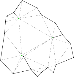
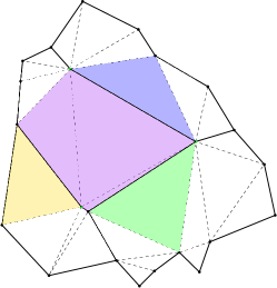
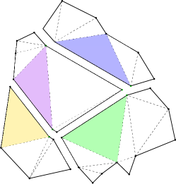
Figure 11: Example of a non-simple polygon split using barrier-edge tips. (a) Non-simple polygon. (b) Middle edges incident to barrier-edge tips labeled as frontier-edges (solid lines) and seed triangles (colorful triangles) stored in the seed list $L_{p}$ and marked as 1 in the $A$ bit array. (c) The four new polygons without barrier-edge tips.

4.5 Computational Complexity Analysis

In this section, we analyze the computational complexity of the whole algorithm. Let $n$ be the initial number of points, $m$ the number of triangles of the input triangulation, $m_{i}$ the number of triangles of the terminal-edge region $R_{i}$ used to generate the simple or non-simple polygon $P_{i}$

1. Label Phase. This phase uses three iterations of cost $O(m)$, one to label longest-edges, one to identify terminal-edges and another to store seed triangles.

2. Traversal Phase. This phase calls Algorithm 2 to build one polygon simple or not simple. The construction of polygon $P_{i}$ has cost $O(m_{i})$. Each triangle is visited three times by Lemma 1 in the worst case (when a triangle does not have frontier-edges). As each terminal-edge region covers the whole domain without overlapping, then this phase costs $O(m)$.

3. Non-simple Polygon Reparation phase. This phase calls Algorithm 3 to divide one non-simple polygon $P_{i}$ into simple ones. By Lemma 2, each triangle $t\in R_{i}$ is visited at most $3$ times, so the computation of $deg(b)$, $\forall b\in R_{i}$ is $O(m_{i})$. The partition of $P_{i}$ into simple polygons has then a cost $O(m_{i})$ because the new simple polygons do not overlap and the algorithm only travels inside their triangles. Finally, the cost to repair all non-simple polygons is bounded $O(m)$.

As result, the computational complexity of the whole algorithm is $O(n)$ ($m=O(n)$). With respect to the memory usage, the cost is $O(n)$ too. The Vertex array has size $2n$, the Triangle and Neighbor arrays have size $3n$. The number of final polygons in the mesh is less than the number of triangles in the input triangulation, i.e., bounded by $m$.

4.6 Impact of the initial triangulation

As mentioned above, the polygons inside a Polylla mesh depend on the initial triangulation. Any triangulation can be used as input. Fig 12 shows three different triangulations for the same point distribution generated using algorithms available in the 2D Triangulations package of the CGAL library cgal:y-t2-21b . Fig. 12 is a Polylla mesh built from the triangulation generated by the incremental algorithm without edge-flips (Fig 12). The Polylla mesh in Fig 12 was built from a regular triangulation BOISSONNAT20025 (a weighted triangulation) with random weights shown in Fig 12, and Fig. 12 shows a Polylla mesh generated from the Delaunay triangulation drawn in Fig 12. As expected, the shape of the resulting polygons is notoriously different. In order to see the differences, Table 1 shows for each mesh, the minimum and maximum interior angle of both the input triangulation and the generated polygon meshes, the number of polygons and the average number of edges per polygon. It can be observed that polygon meshes have a minimum interior angle greater than the minimum angle of the corresponding triangulation. Since the Polylla algorithm joins triangles to generate polygons, the lower bound for the minimum interior angle of any polygon is the minimum angle of the input triangulation. In the case of maximum angles, the maximum angle of a Polylla mesh is usually larger than the maximum angle of the input triangulation because a Polylla’s polygons can be nonconvex polygons. It seems that Polylla meshes generated from Delaunay triangulations tends to contain less polygons and polygons defined with more edges than the ones obtained from other triangulations. Further research is necessary to probe these findings.

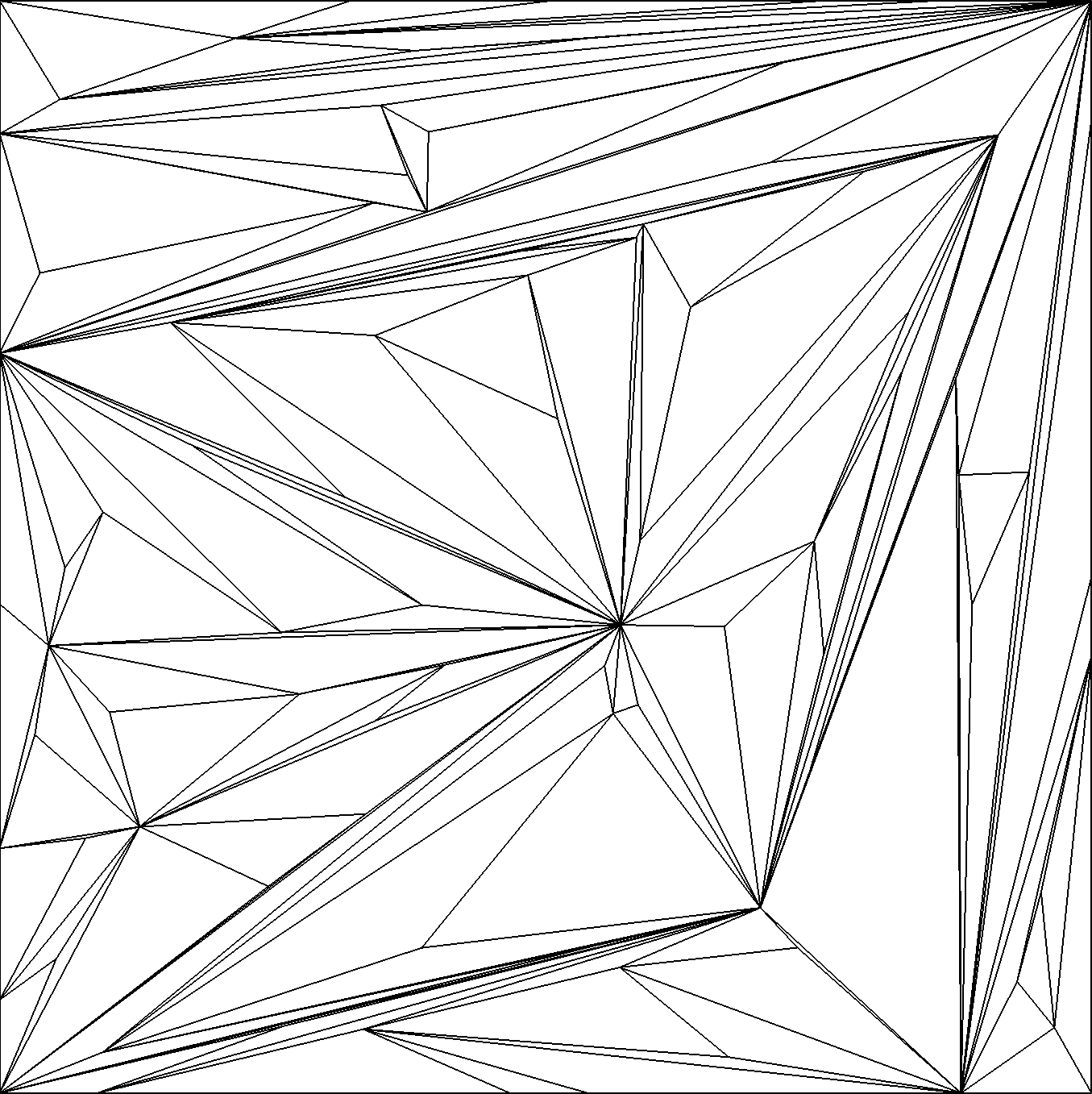
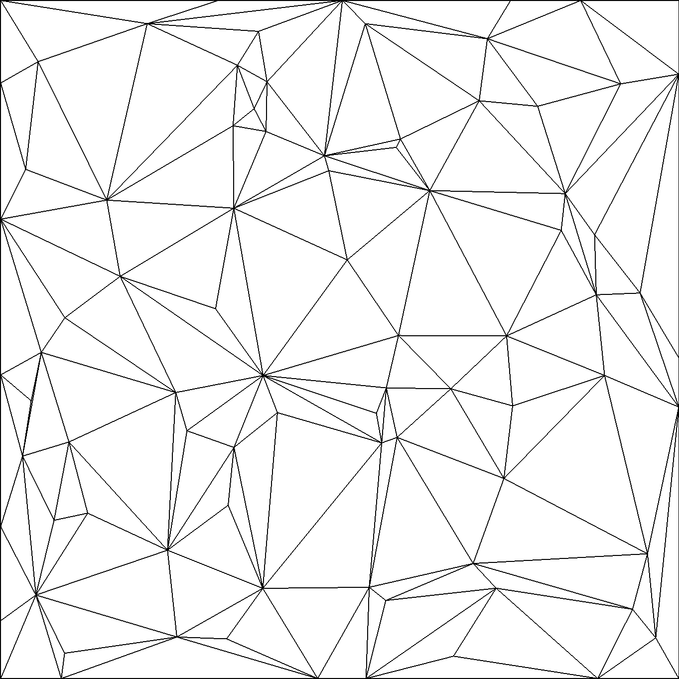
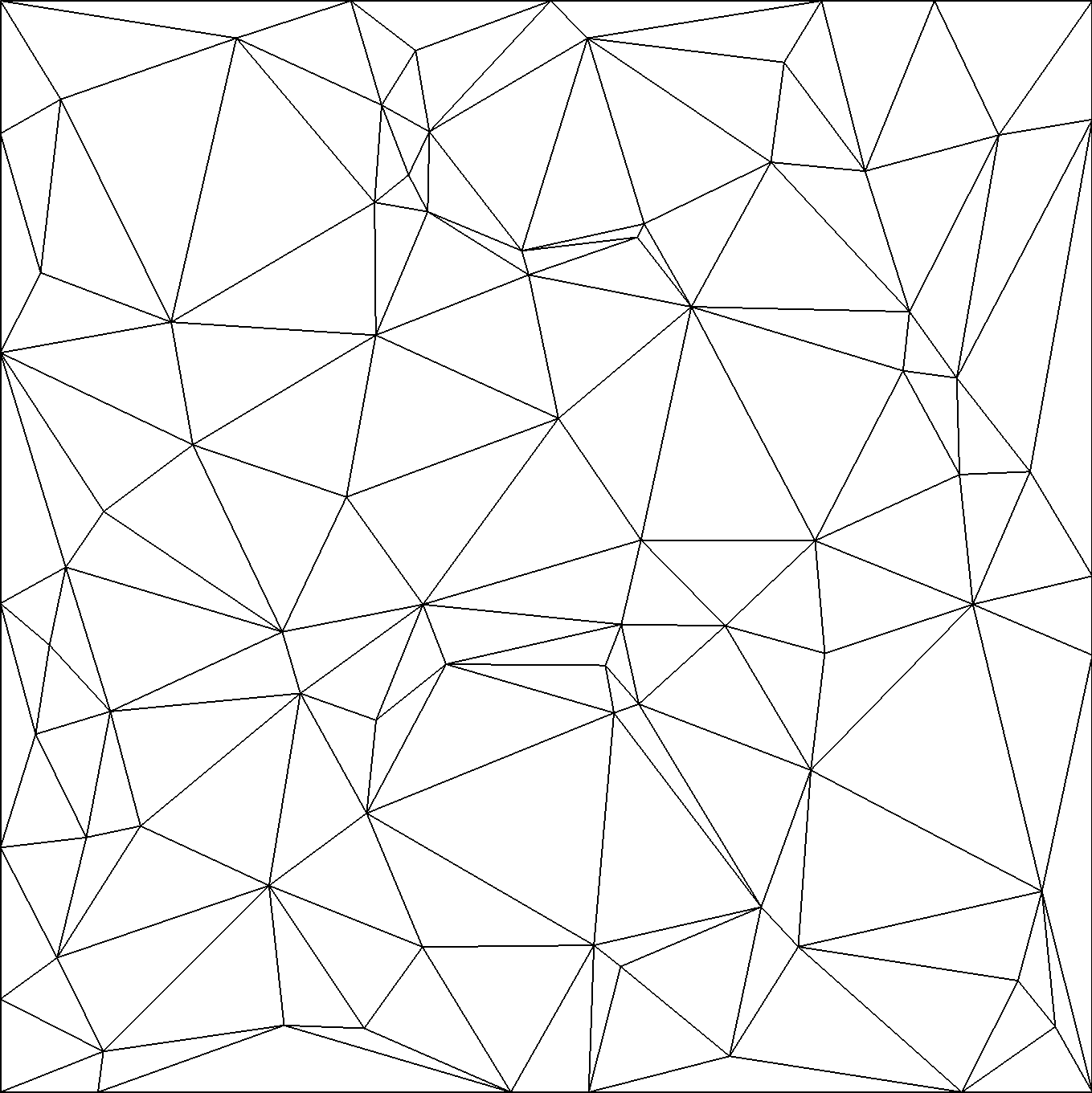
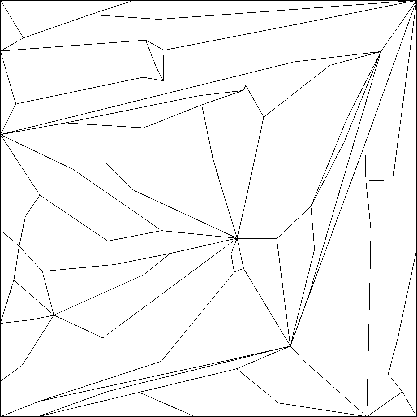
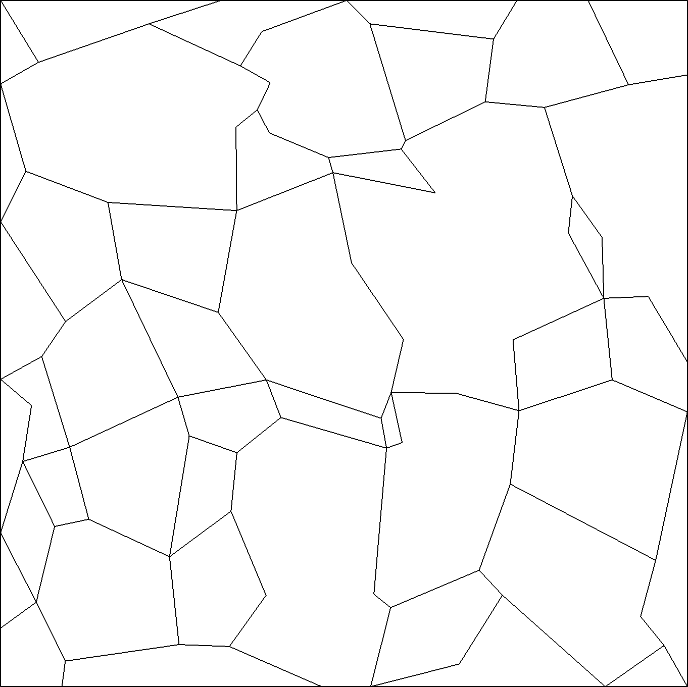
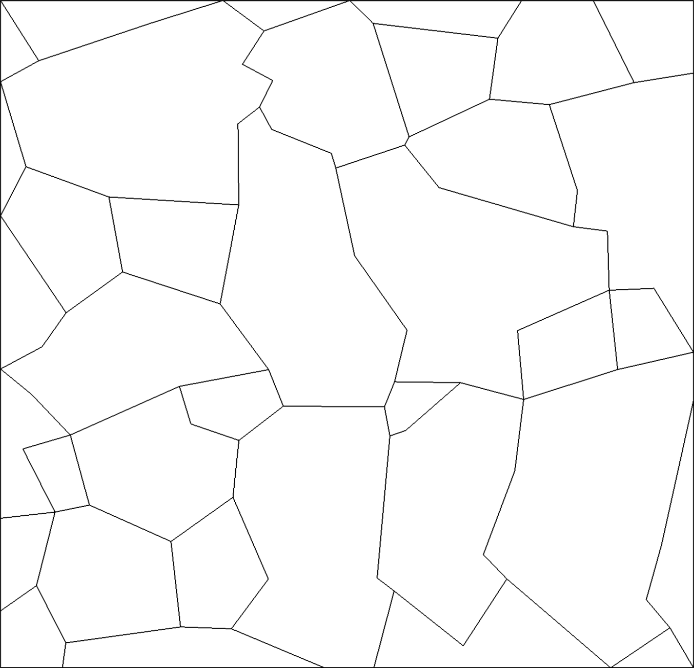
Figure 12: Polylla meshes generated from different kind of initial triangulations over the same input points. Triangulations were generated using the 2D Triangulations package of CGAL library cgal:y-t2-21b . (a) Triangulation generated by the incremental algorithm, (b) regular triangulation generated using random weights, (c) Delaunay triangulation, (d) Polylla mesh generated from the triangulation (a), (e) Polylla mesh generated from the triangulation (b), and (f) Polylla mesh generated from the triangulation (c).

	Delaunay Triangulation		Polylla Mesh
	Min Angle	Max Angle	Polylla’s Polygons	Min Angle	Max Angle	Edges per Polygon
Incremental Triangulation	0.027	179.87	41	0.36	303.16	5.65
Regular Triangulation	1.36	177.09	45	12.04	318.98	5.33
Delaunay Triangulation	5.75	158.61	36	12.04	279.22	6.16

Table 1: Geometric information of the Polylla meshes generated from different triangulations from the same point set (150 points).

It is worth to mention that since the Polylla algorithm takes as input a triangulation, it can process any geometry domain that can be triangulated. This includes complex geometries with holes as shown in Fig 13. In particular, Fig. 13 shows a geometry specified as a planar straight line graph (PLSG) obtained from triangle2d . Fig. 13 is a Polylla mesh generated from a constrained Delaunay triangulation of 13. Fig. 13 shows a Polylla mesh from a refined conforming Delaunay triangulation of 13. Grey polygons are holes. The algorithm considers the edges of the holes as border edges. Meshes generated from complex geometries representing Chilean geographic regions can be seen in Appendix A.

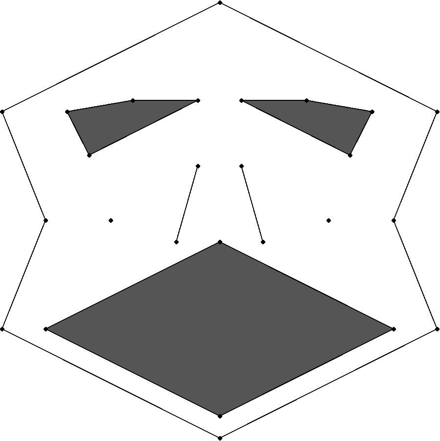
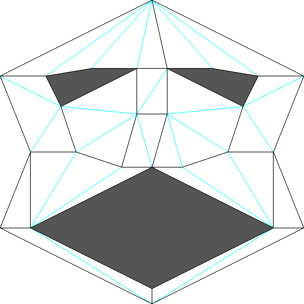
Figure 13: Polylla mesh generated from the PLSG description of the Face taken from triangle2d . The edges of the initial triangulation are drawn using black and cyan colors. (b) Polygonal mesh obtained from the constrained Delaunay triangulation of the input geometry (26 vertices). (c) Polygonal mesh generated from a refined Delaunay triangulation with 220 vertices.

5 Polylla meshes vs Voronoi based meshes

Currently, if polygonal meshes different from triangulations or quad meshes are required to solve some scientific or engineering problems, constrained Voronoi meshes are chosen. We believe that the polygonal meshes generated by Polylla can be an alternative to Voronoi meshes when researchers and engineers would like to model domains using arbitrary polygon shapes. That is why in this section we show standard statistics of these new polygonal meshes in contrast to constrained Voronoi meshes. The C++ implementation of Polylla used for the experiments can be downloaded from this repository.

The experiment was designed as follows: the domain is a square with a set of random points in its interior varying from $10^{2}$ to $10^{6}$. A tolerance $\pm\gamma$ is defined and used in case of a point $p$ is too close to one square side; in that case the point $p$ is inserted in the border edge. The statistics of the polygonal meshes generated by Polylla starting from Delaunay triangulations generated by using Detri2 Detri2 are summarized in Table 2. In the case constrained Voronoi meshes, Deldir deldir was used to generate the meshes and to obtain their mesh information. The statistics for the same initial points (sites) are presented in Table 3.

Input points	Triangles	Terminal-edge regions	Polylla polygons	Maximum barrier-edge tips in non-simple polygons	Barrier-edge tips	Average triangles per polygon	Average polygon vertices
10	9	3	3	0	0	3.00	6.67
$10^{2}$	180	35	38	1	3	4.74	6.89
$10^{3}$	1911	281	305	2	24	6.27	8.30
$10^{4}$	19768	3034	3228	4	194	6.12	8.13
$10^{5}$	199163	30288	32271	4	1984	6.17	8.17
$10^{6}$	1997497	302944	322561	4	19647	6.19	8.19

Table 2: Geometric information of Polylla mesh

Input Points	Voronoi vertices	Voronoi Regions	Voronoi Edges	Edges per Region
10	22	10	31	4.90
$10^{2}$	202	100	301	5.75
$10^{3}$	2002	1000	3001	5.90
$10^{4}$	20001	10000	30001	5.96

Table 3: Geometric information of constrained Voronoi diagram

In Table 2, we can observe that over $10^{4}$ input points, the number of initial triangles per polygon is $6.5$ and the number of vertices per polygon is $8.5$, both values on average. The number of barrier-edge tips is less than $3\%$ of the number of points, so the reparation phase just adds less than $10\%$ of polygons to the mesh. If we compare Polylla meshes with the meshes generated from the Voronoi diagram, the constrained Voronoi meshes contain 3 times more polygons than our meshes. Each Voronoi region based polygon is delimited in average by 6 edges and Polylla polygons by 8 edges. Moreover, the Polylla meshes use only the points given as input; in contrast, the Voronoi based meshes use new points, the Voronoi points, one per each triangle of the Delaunay mesh. Since the number of triangles is greater than the number of input points, the size of the Voronoi mesh is greater than the size of the Polylla mesh not only in terms of polygons, but also in terms of mesh points.

It is worth mentioning that a Polylla mesh does not need to insert extra-points at the boundary to fit the domain geometry; in contrast the constrained Voronoi mesh includes new points at the boundary/interfaces inserted while cutting the Voronoi regions that go outside the domain.

We have also evaluated the time performance of Polylla. The results shown in Fig. 14 were made on Patagón, a computer with two Intel Xeon Platinum 8260 of 2.4Ghz, located at the Universidad Austral de Chile patagon-uach . The results are the average time of five program executions with same data-set in a different core. The time of each phase is included together with time to generate the initial triangulation. Of the three phases described in section 4, the phase that takes less time is the non-simple polygon reparation phase. The main reason is that the number of terminal-edge regions with barrier edges is around 1% of the total number terminal-edges regions formed from random point sets as can be seen in Fig. 14. The time of the Label phase is higher than the time of the traversal phase. This can be explained due to the use of floating-point arithmetic to calculate the length of each edge and so to assign the proper label.

In order to compare the CPU time required to generate constrained Voronoi and Polylla meshes, we looked for free and open source tools. The CGAL library provides 2D Voronoi Diagram Adaptor package cgal:k-vda2-21b to generate Voronoi diagrams, but this package does not provide a method to cut Voronoi regions against the domain boundary. So we implemented a function to do this process. In contrast, Detri2 Detri2 offers a robust method to generate constrained Voronoi meshes. Table 4 shows the cpu-times in seconds needed to generate polygonal meshes using Polylla, Detri2D and CGAL from 100000, 500000 and 1000000 points over a L-shape domain. Experiments were run in a CPU Intel(R) Core(TM) i5-9600K of 3.70GHz. Detri2d computes the CDT first and then the CVD from the CDT. That is why we included the time to generate the CDT separated from the generation of the CVD. The Polylla time includes only the time spent in the three phases that processes the input triangulation to generate the polygon mesh. The CGAl algorithm to generate the VD includes generation of the Delaunay triangulation first and from this triangulation computes the Voronoi Diagram. The CVD cost in CGAL is the sum of VD and CV. This preliminary comparison shows that the time to generate a CDT using Detri2d or CGAL plus the time Polylla takes to generate the polygonal mesh is much less than the time needed for generating a CVD either using Detri2 or the CGAl library. The main reason is that constrained Voronoi based meshing algorithms require to compute and insert new points (Voronoi points), to cut Voronoi regions and insert new boundary points. In contrast, the Polylla algorithm just needs to process the vertices, edges and triangles of the input triangulation. The domain boundary is already represented by some triangle edges.

		Detri2		CGAL
Vertices	Polylla	CDT	CVD	CDT	VD	CV	CVD
100000	0.193	0.326	229.489	1.712	28.39	9.68	38.07
500000	0.7684	1.703	5736.473	9.006	335.26	56.16	391.42
1000000	1.3294	3.346	21341.734	16.082	870.52	120.52	991.04

Table 4: Time comparison, in seconds, of Polylla vs Constrained Voronoi Diagram (CDV) using Detri2 and CGAL. CDT is the time to generate a Constrained Delaunay Triangulation, VD is the time of generate Voronoi Diagram, CV is the time need to cut all regions of Voronoi Diagram and CVD is the total time of generate the Constrained Voronoi Diagram.

Figure 14: Time performance of the different algorithm phases. The label Polylla mesh indicates the time of the three phases.

Figure 15: Meshes generated from 1000 random points. (a) Polylla mesh.(b) Constrained Voronoi mesh generated with Detri2qt Detri2 .

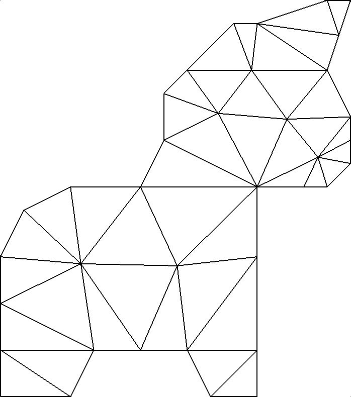
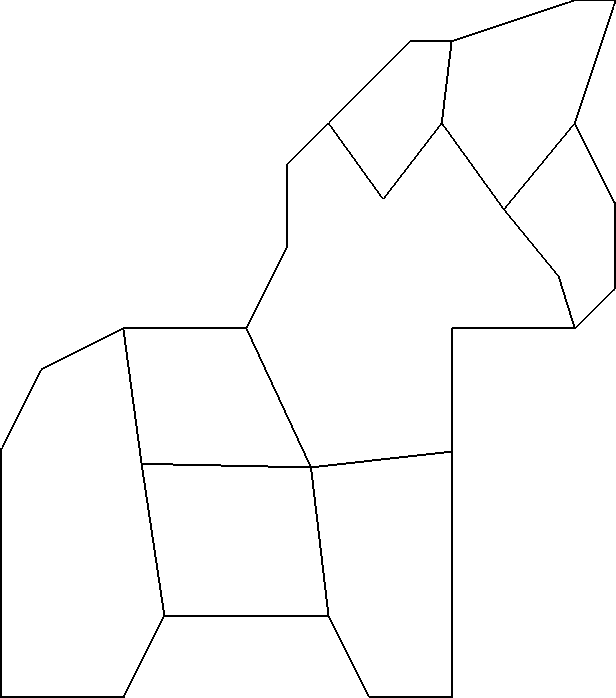
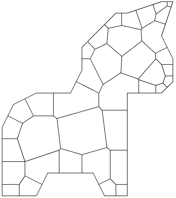
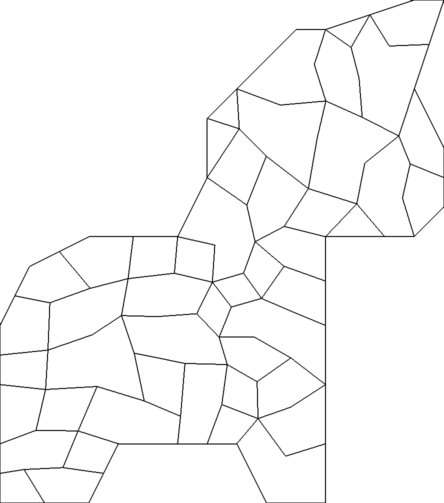
Figure 16: Qualitative comparison using an Unicorn PLSG as input AlejandroNUA2019 (a) Triangulation of unicorn PLSG with 36 vertices. (b) Polylla mesh includes exactly the 36 input vertices. (c) The constrained Voronoi mesh requires 100 vertices to model the same input. (d) Polylla mesh from a refined Delaunay triangulation with 100 vertices.

In Fig. 15 a qualitative comparison between a Polylla mesh and a constrained Voronoi mesh can be observed. Both meshes were generated from the same initial random point set. Fig. 15 shows the polygonal mesh generated by Polylla and Fig. 15 the constrained Voronoi mesh generated by Detri2qt. Some other examples of polygonal meshes generated for non convex domains are shown in Fig. 13 and Fig. 16.

Fig. 16 shows polygonal meshes for an Unicorn example generated by both the Polylla (Fig. 16) and Detri2qt (Fig. 16) tools. The initial triangulation and interior points are shown in Fig. 16. As expected, the constrained Voronoi mesh contains more points (100 vertices) and polygons than the Polylla mesh as shown in Fig. 16. Just for a qualitative comparison, we used Polylla to generate a polygonal mesh from 100 vertices and this mesh is shown in Fig. 16.

6 Preliminary Simulation Results

In this section, we assess the Polylla meshes using the virtual element method (VEM) Basisprinciples . To this end, an L-shaped domain is considered. Fig. 17 shows this domain meshed with a random and a semiuniform Polylla sample mesh. For comparison purposes, we also consider random and semiuniform Voronoi meshes (sample meshes are depicted in Fig. 18). The chosen problem is governed by the Laplace equation and its exact solution is given by MITCHELL2013350

$$u(x_{1},x_{2})=r^{2/3}\sin(2/3\,\theta),\quad r=\sqrt{x_{1}^{2}+x_{2}^{2}},\quad\theta(x_{1},x_{2})=\arctan(x_{2}/x_{1}).$$

The boundary conditions are of Dirichlet type with the exact solution imposed on the entire domain boundary. The re-entrant corner of the L-shaped domain introduces a singularity in the solution that manifests itself as unbounded derivatives of $u$ at the origin. The numerical solution (denoted by $u_{h}$) is assessed through its convergence with mesh refinements. Figs. 19 and 20 present the $L^{2}$ norm and the $H^{1}$ seminorm of the error, where it is shown that the VEM on Polylla (random and semiuniform) and Voronoi (random and semiuniform) meshes delivers accurate solutions with optimal convergence rates of 2 (for the $L^{2}$ norm) and 1 (for the $H^{1}$ seminorm).

The performance of VEM using Polylla (random and semiuniform) and Voronoi (random and semiuniform) meshes are compared in Fig. 21, where the $H^{1}$ seminorm of the error and the normalized CPU time are each plotted as a function of the number of degrees of freedom (DOF). The normalized CPU time is defined as the ratio of the CPU time of a particular simulation to the maximum CPU time found for any of the simulations that were run. Each of the four set of meshes (random Polylla, semiuniform Polylla, random Voronoi and semiuniform Voronoi) consists of four meshes of increasing number of degrees of freedom. Therefore, in total, there are sixteen meshes in the study.

The CPU time is measured from the reading of the mesh until the solution of the system of equations is ended. Each mesh is run ten times and the CPU time recorded is the average CPU time. From Fig. 21 it is observed that for equal number of degrees of freedom similar accuracy and computational cost are obtained for the four set of meshes.

Finally, for completeness of the presented numerical results, contour plots of the VEM solution on Polylla meshes are shown in Figs. 22 and 23 for the $u_{h}$ and $\bm{\nabla}u_{h}$ fields, respectively.

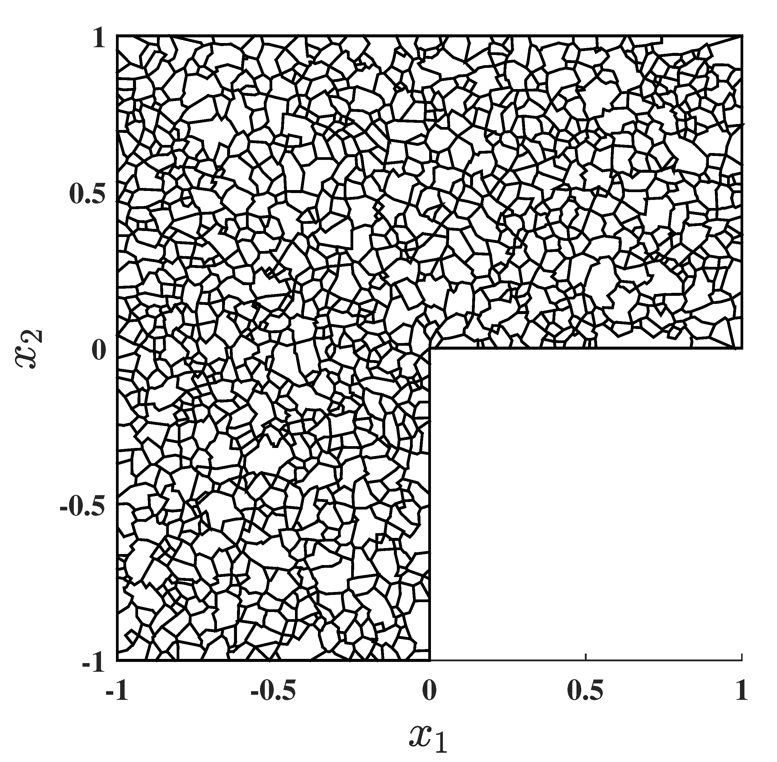
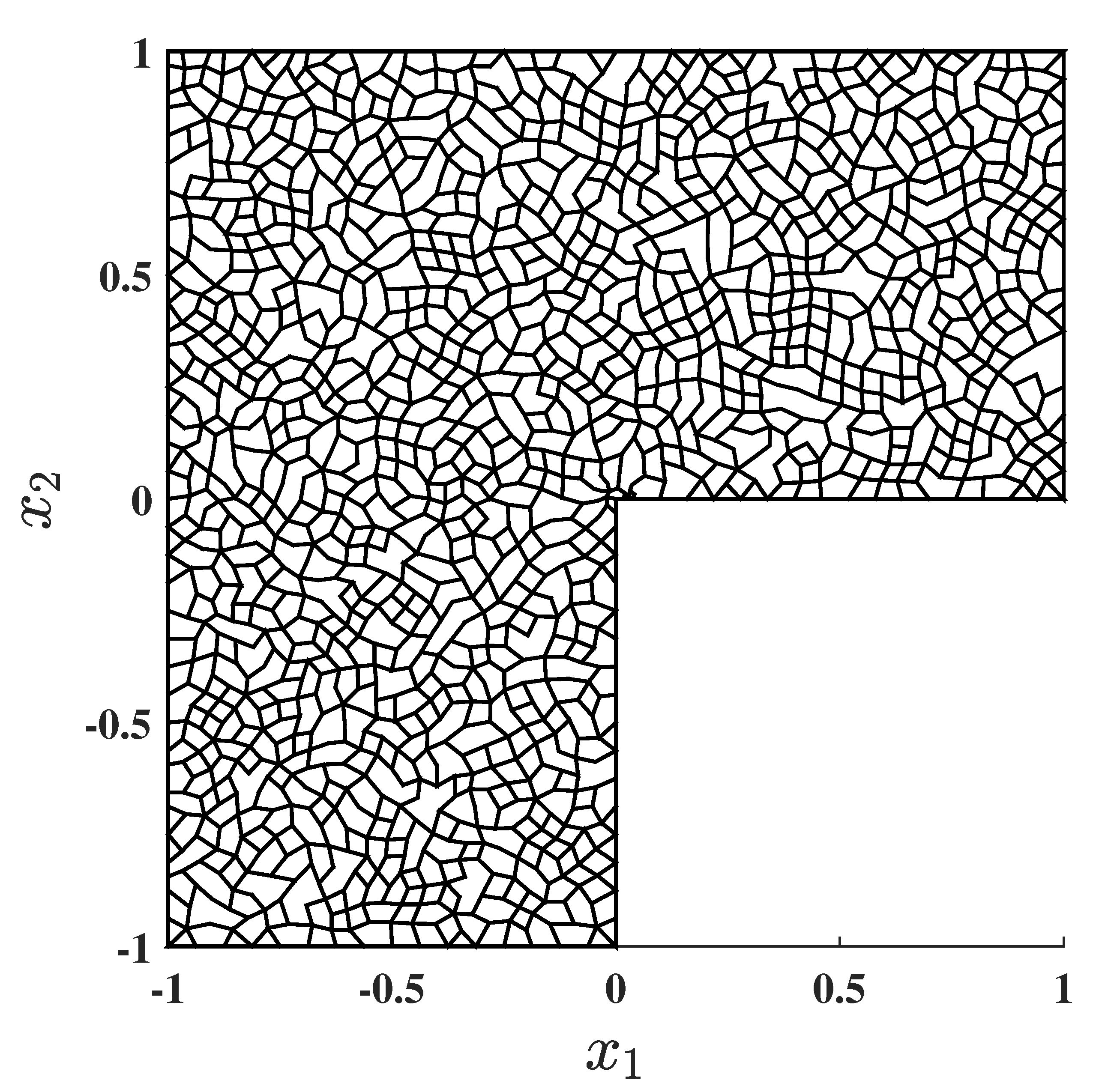
Figure 17: L-shaped domain meshed with (a) a random and (b) a semiuniform Polylla mesh.

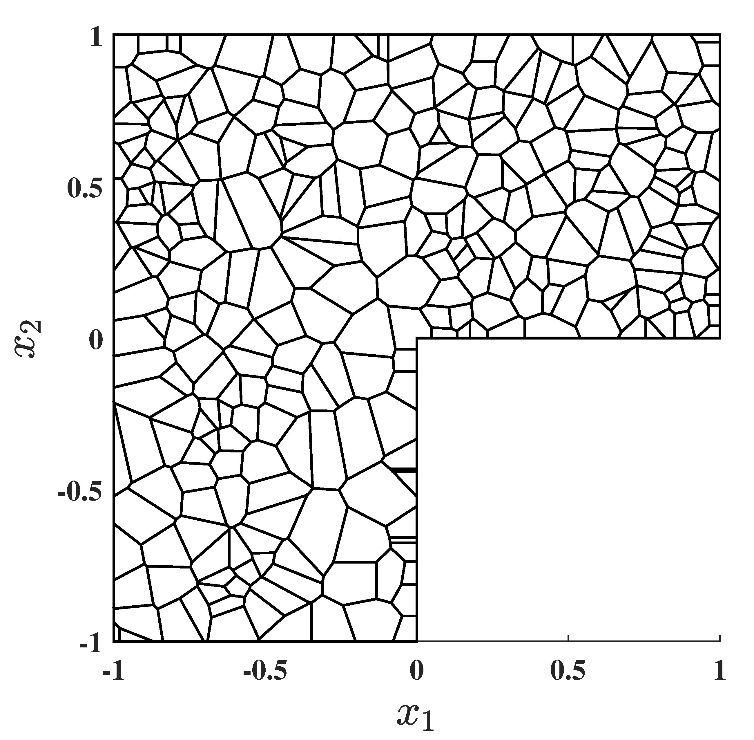
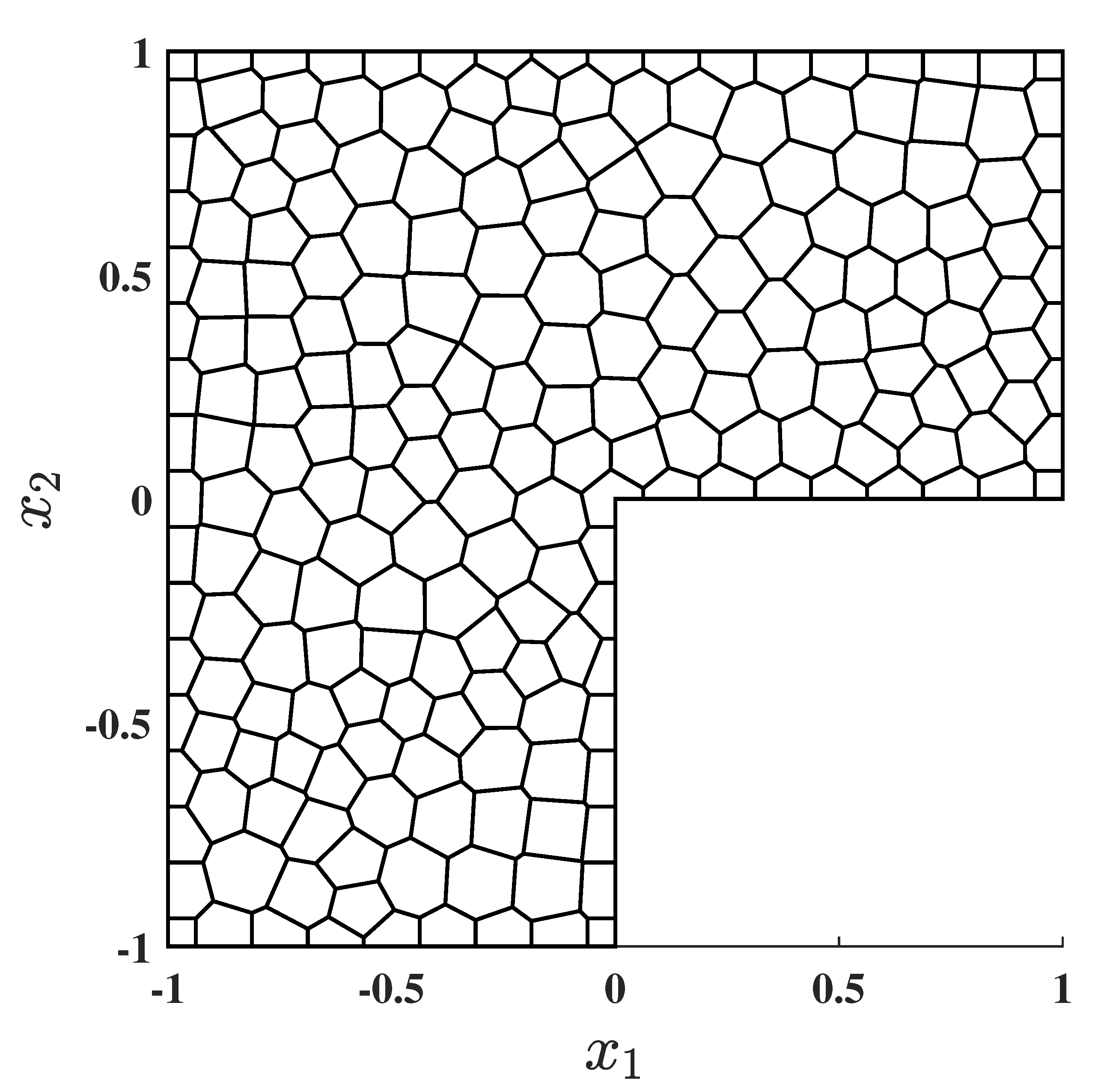
Figure 18: L-shaped domain meshed with (a) a random and (b) a semiuniform Voronoi mesh.

Note that random Polylla meshes (Fig 17) were generated from constrained Delaunay triangulation built over a L-shaped domain with points randomly generated in its interior. Semiuniform Polylla (Fig 17) meshes were generated from a conforming Delaunay triangulation using pygalmesh Schlomer_pygalmesh_Python_interface . To generate the same number of triangles as the random mesh, an arbitrary maximum edge size constraint was given as input. The random (Fig 18) and semiuniform (Fig 18) Voronoi meshes were generated from the points (sites) of both the constrained Delaunay triangulation and the conforming Delaunay triangulation, respectively. Next, each infinite Voronoi region was intersected with the L-shaped domain to generate the constrained Voronoi mesh.

   

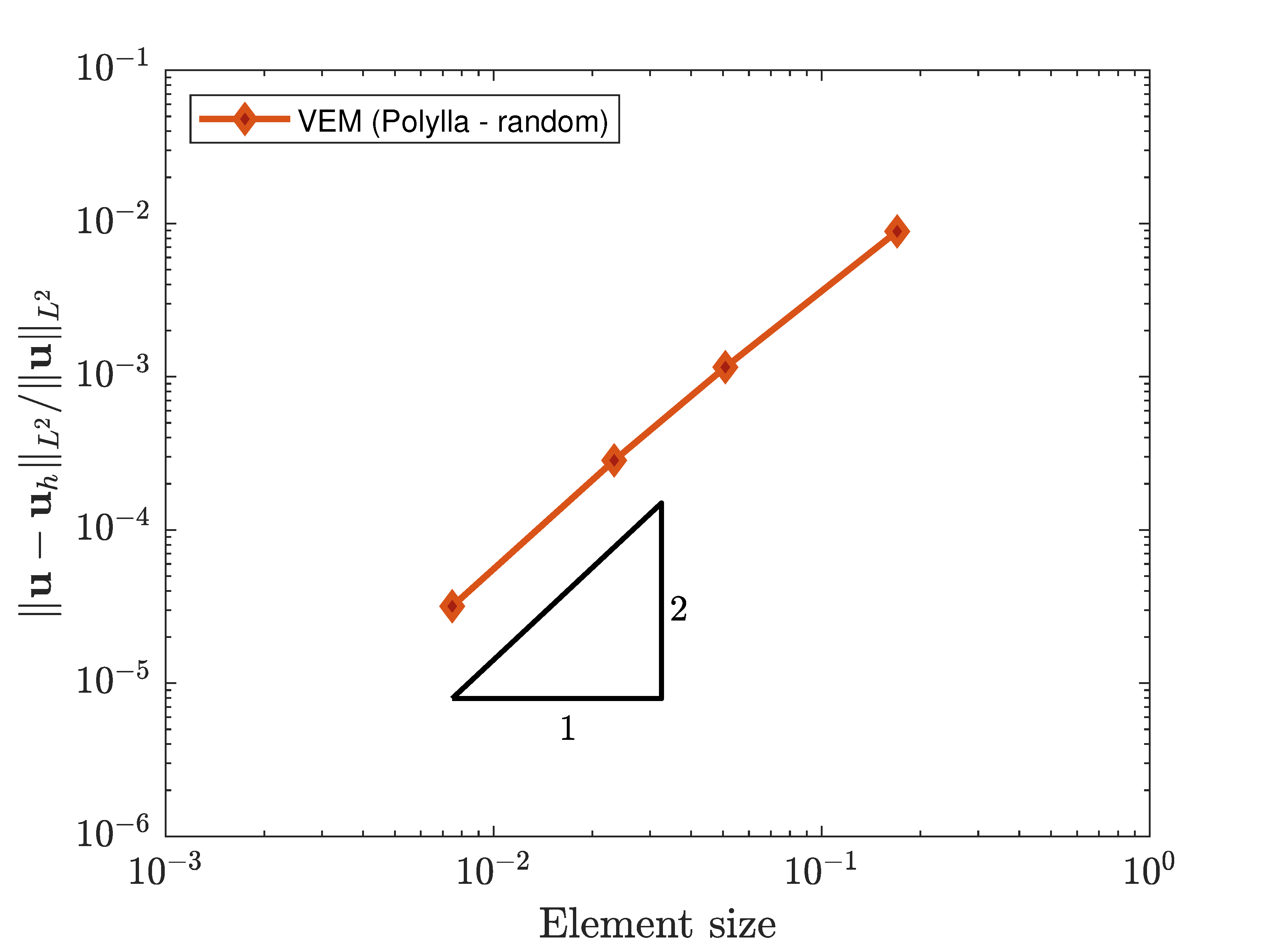
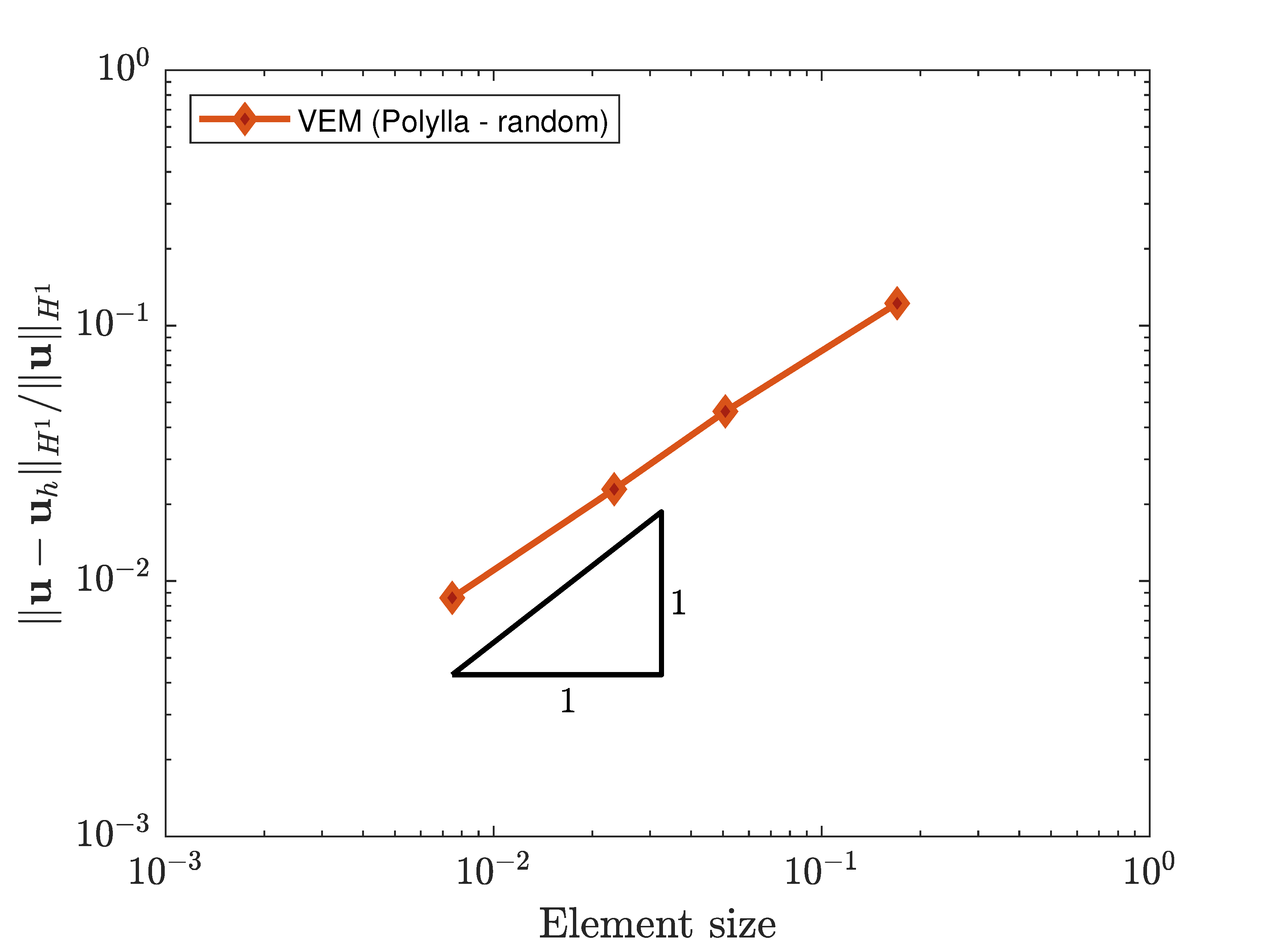
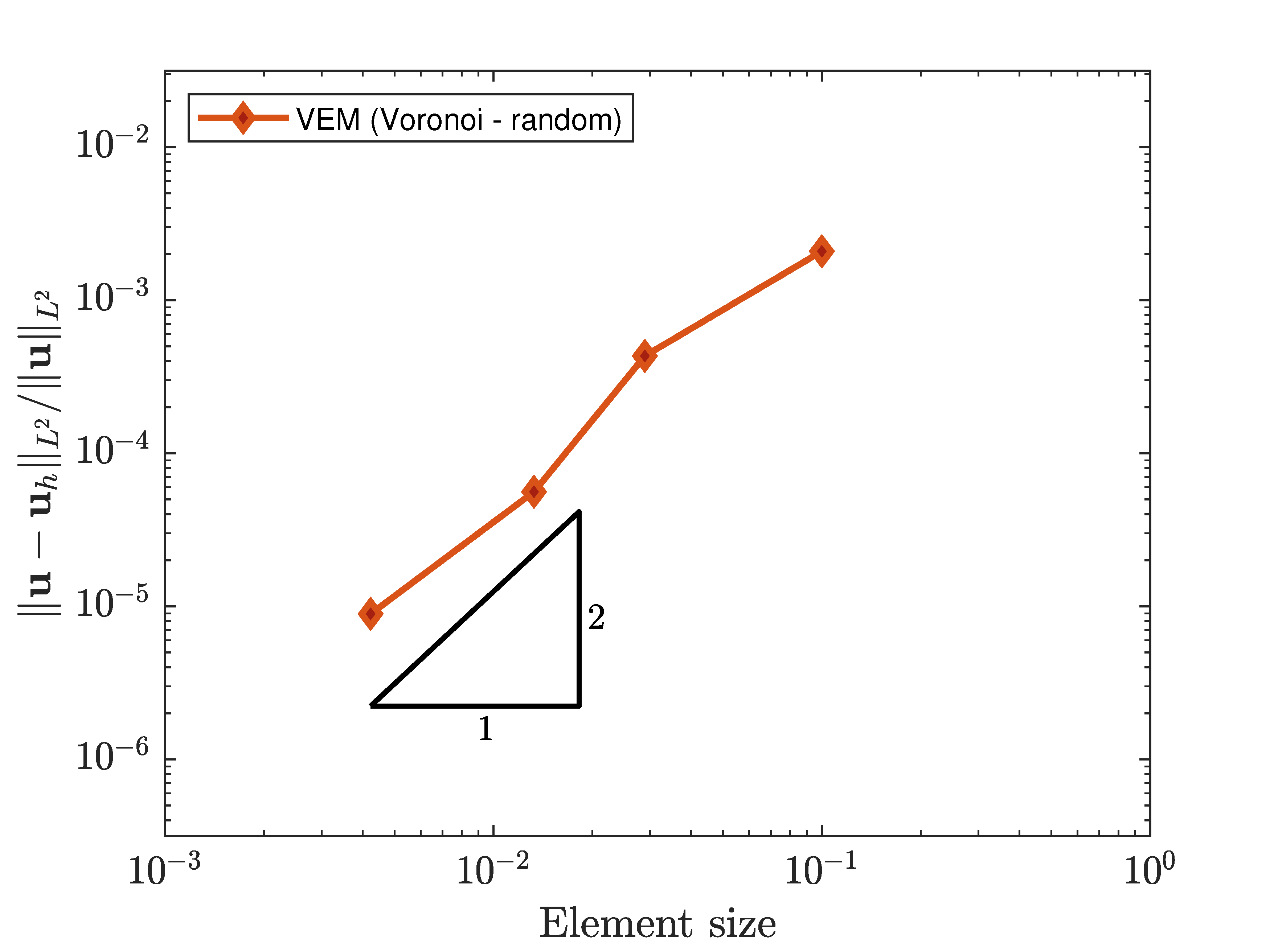
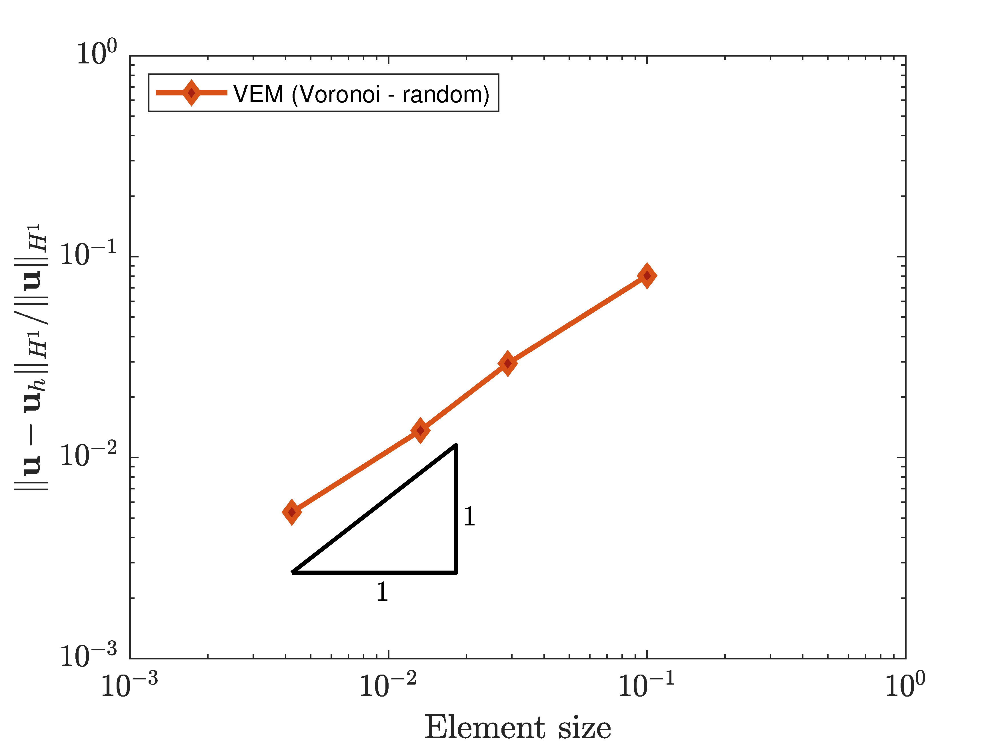
Figure 19: $L^{2}$ norm and $H^{1}$ seminorm of the error using the VEM on random Polylla meshes ((a) and (b), respectively), and on random Voronoi meshes ((c) and (d), respectively).

   

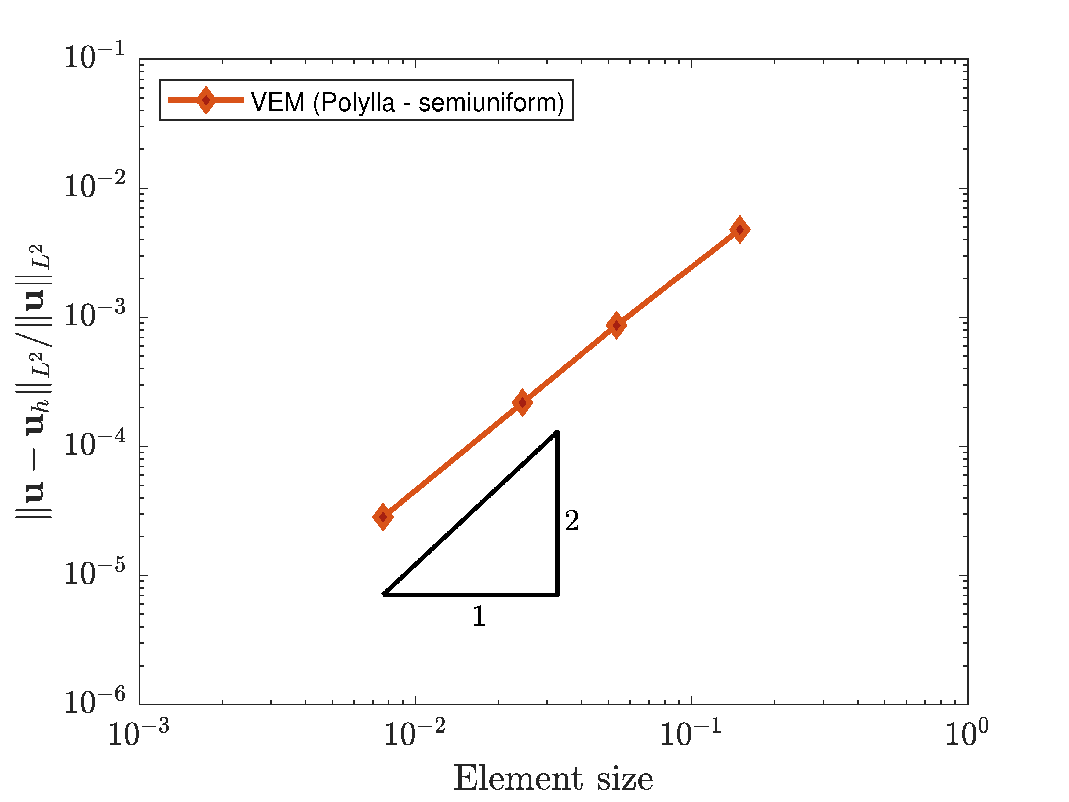
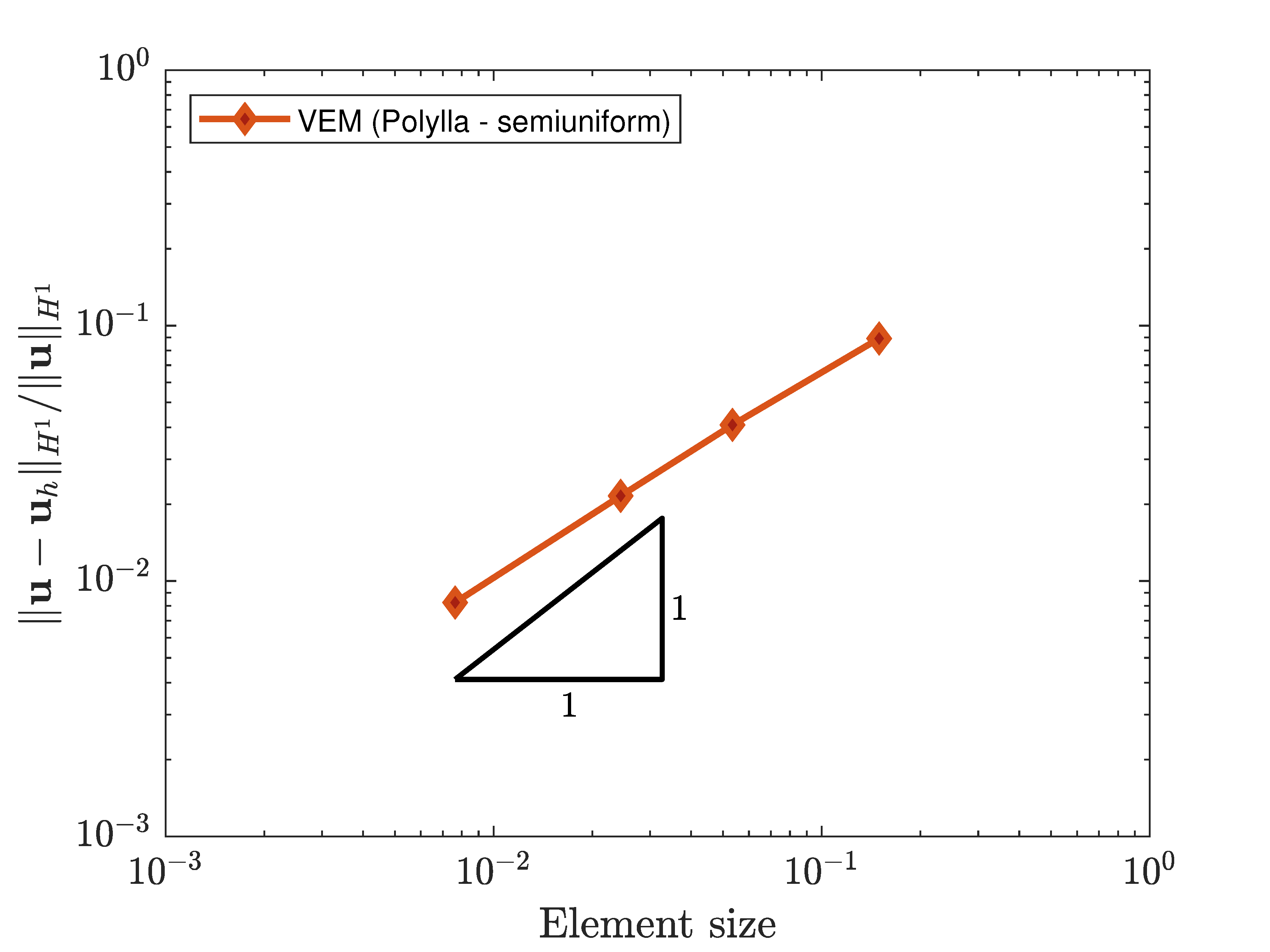
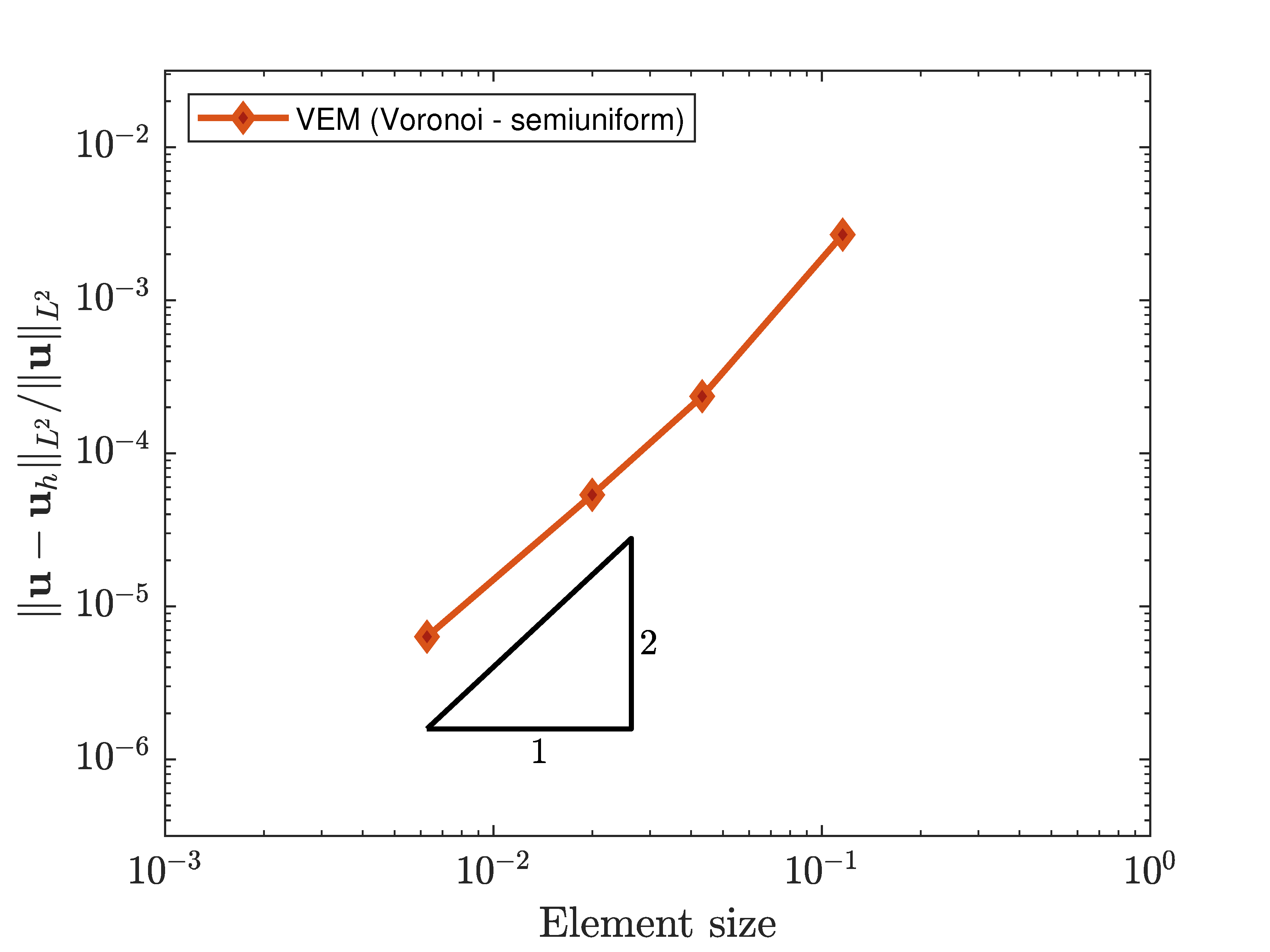
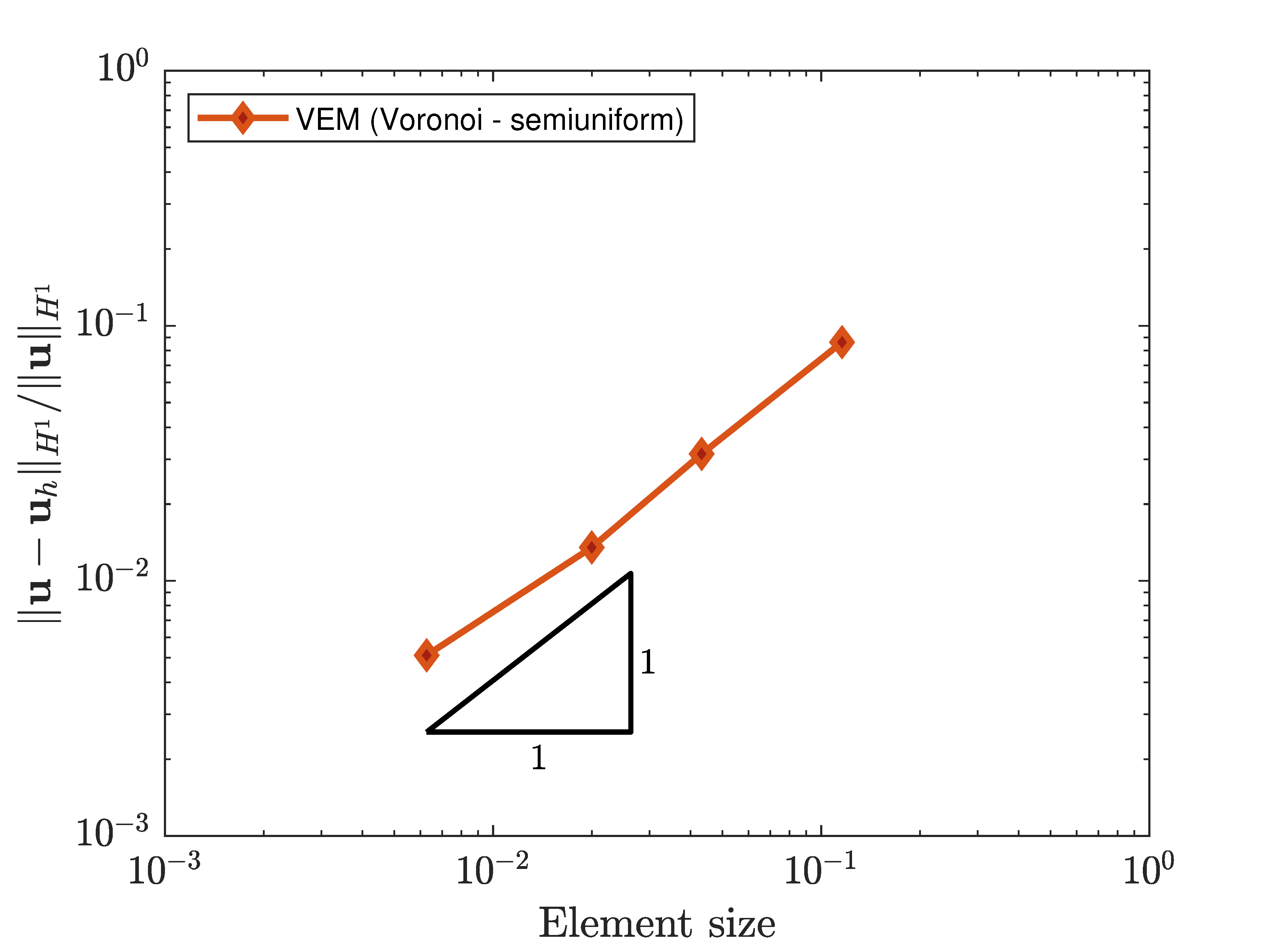
Figure 20: $L^{2}$ norm and $H^{1}$ seminorm of the error using the VEM on semiuniform Polylla meshes ((a) and (b), respectively), and on semiuniform Voronoi meshes ((c) and (d), respectively).

 

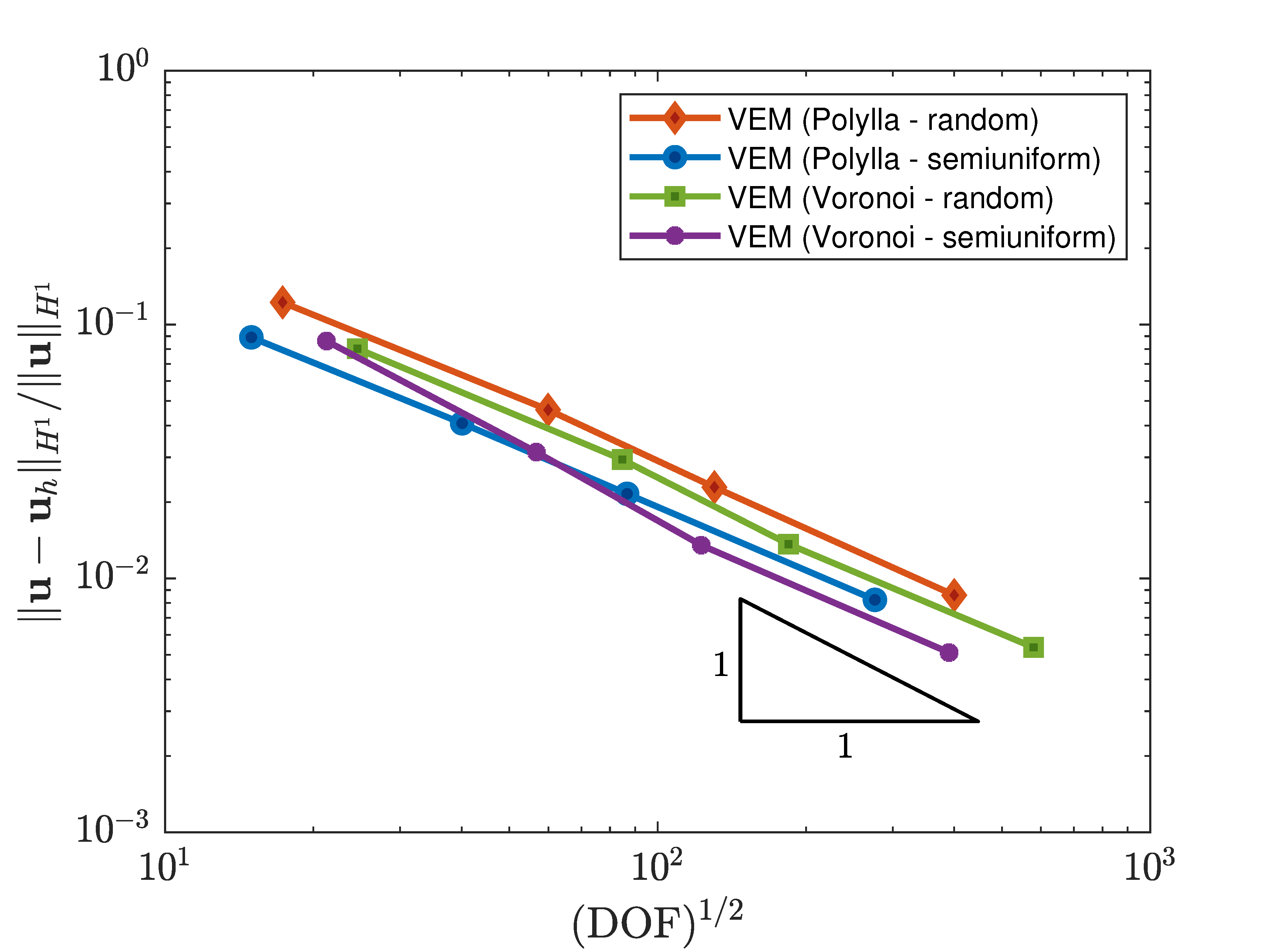
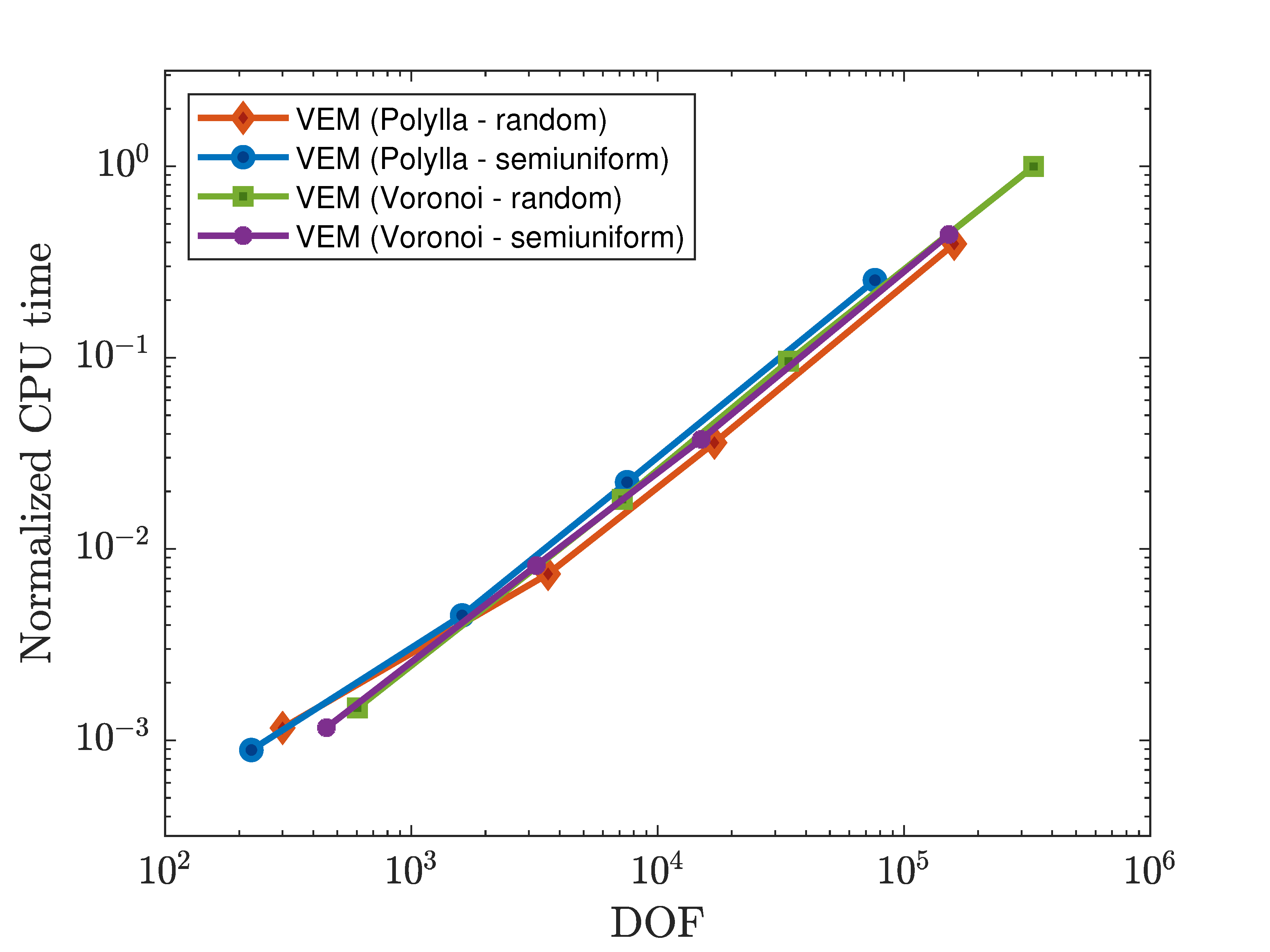
Figure 21: Performance of the VEM using Polylla and Voronoi meshes. (a) $H^{1}$ seminorm of the error and (b) CPU time as a function of the degrees of freedom (DOF).

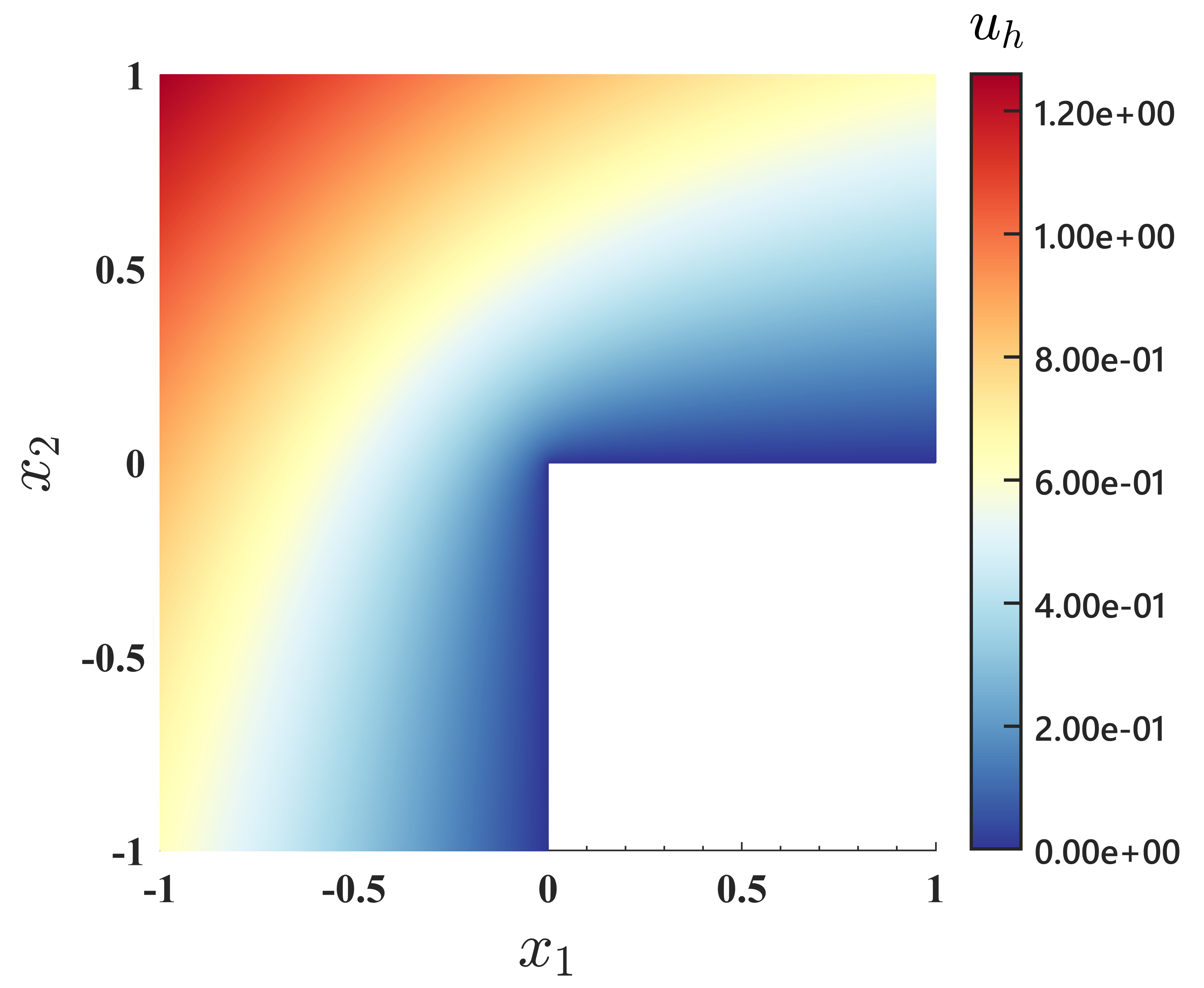
Figure 22: Contour plots of the VEM solution for the $u$ field. (a) Random and (b) semiuniform Polylla meshes.

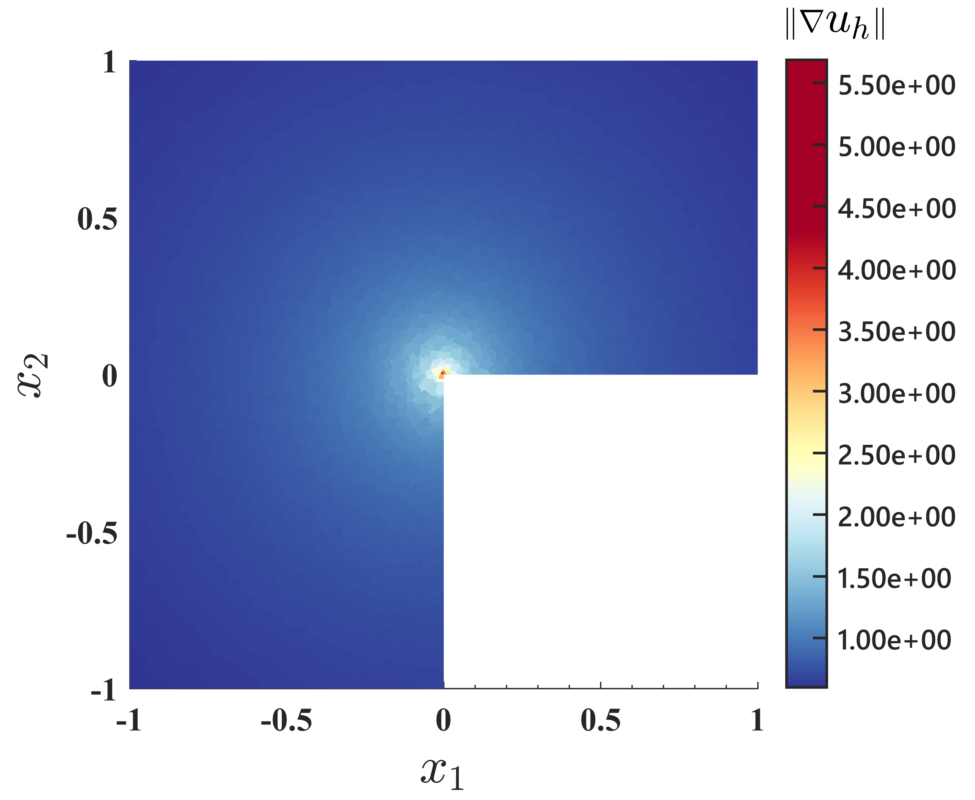
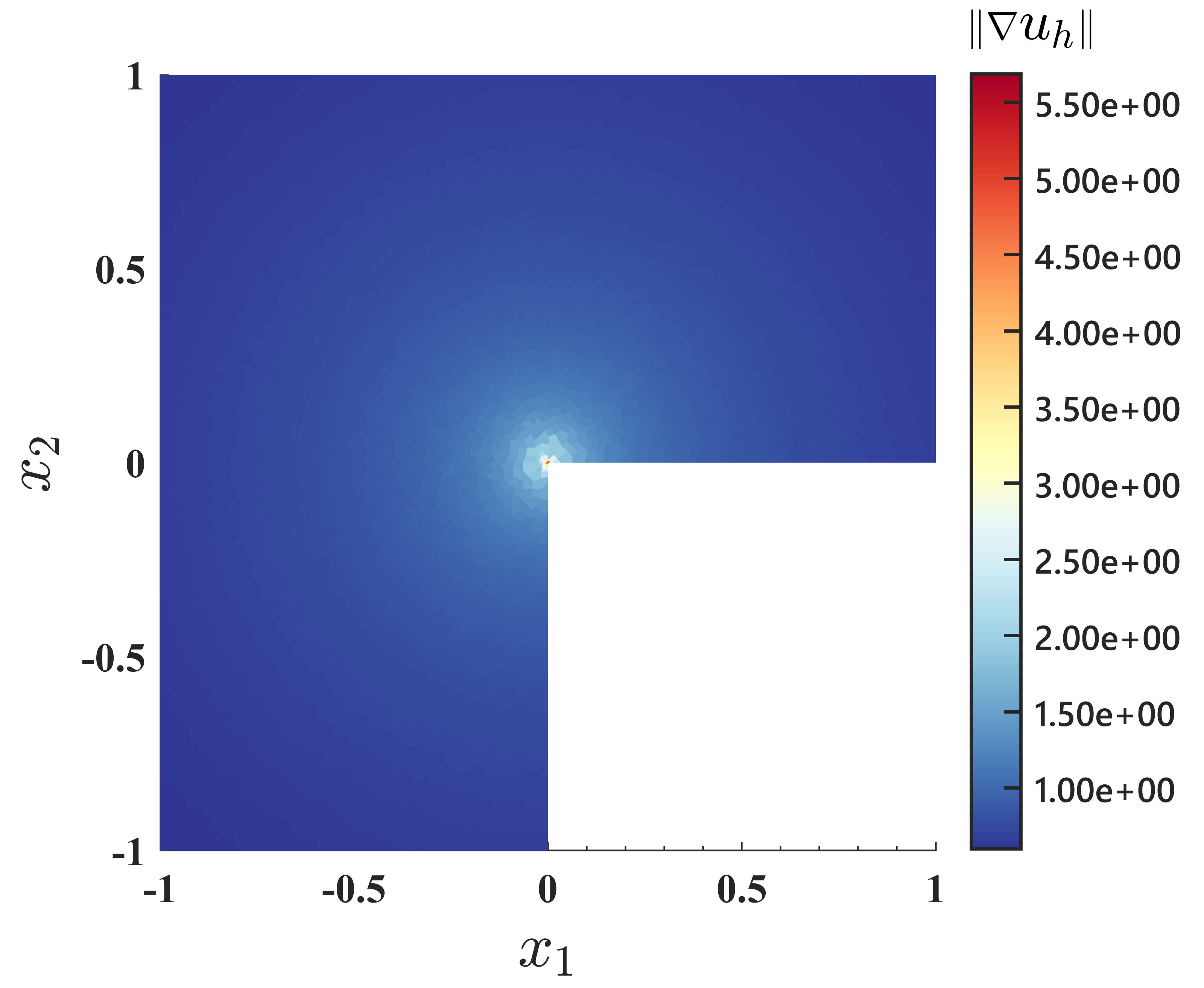
Figure 23: Contour plots of the VEM solution for the $\bm{\nabla}u$ field. (a) Random and (b) semiuniform Polylla meshes.

7 Conclusions and ongoing work

We have presented Polylla, an algorithm to generate a new kind of polygonal mesh using terminal-edge regions. The proposed algorithm takes as input a triangulation with the required point density and generates a polygonal mesh without inserting new points. This generated mesh contains three times less polygons and half the number of points than the standard polygonal meshes based on the Voronoi diagram generated from the same input.

Some preliminary simulations were presented and the numerical results showed that the accuracy and computational cost of the VEM numerical solution using Polylla and Voronoi meshes are similar. We think that the advantage of Polylla meshes over Voronoi meshes lies in the mesh generation process, where, once the initial triangulation is available, Polylla meshes are simpler and faster to generate since these meshes do not require any addition or removal of vertices.

The ongoing work is devoted to adding more capabilities to Polylla. In particular, since the algorithm retains the underlying triangulation during the polygon construction, we plan to allow further refinements inside the polygonal mesh in a forthcoming version of Polylla. We also are in the process of developing an extension of the Polylla algorithm to polyhedral meshes using terminal edge-regions in 3D HerviasHCF13 .

8 Acknowledgements

This research was supported by the Patagón supercomputer of Universidad Austral de Chile (FONDEQUIP EQM180042). The second author thanks to Fondecyt project No 1211484 and the first author to Anid doctoral scholarship 21202379.

Declarations

Some journals require declarations to be submitted in a standardised format. Please check the Instructions for Authors of the journal to which you are submitting to see if you need to complete this section. If yes, your manuscript must contain the following sections under the heading ‘Declarations’:

• Funding: This project was funded by Fondecyt Grant No 1211484 and Anid doctoral scholarship 21202379.

• Conflict of interest/Competing interests (check journal-specific guidelines for which heading to use): The authors report no conflict of interest.

• Ethics approval : Not applicable

• Consent to participate : Not applicable

• Consent for publication : Not applicable

• Availability of data and materials : https://github.com/ssalinasfe/Polylla-Mesh

• Code availability: Not applicable https://github.com/ssalinasfe/Polylla-Mesh

• Authors’ contributions : Not applicable

If any of the sections are not relevant to your manuscript, please include the heading and write ‘Not applicable’ for that section.

Editorial Policies for:

Springer journals and proceedings: https://www.springer.com/gp/editorial-policies

Nature Portfolio journals: https://www.nature.com/nature-research/editorial-policies

Scientific Reports: https://www.nature.com/srep/journal-policies/editorial-policies

BMC journals: https://www.biomedcentral.com/getpublished/editorial-policies

Appendix A Complex geometries

This appendix presents some examples of Polylla meshes generated using cartography maps obtained from the Library of National Congress of Chile , and the library PyShp . This library was used to read the .shp files, generate the PSLGs and store the information in .poly files. Fig 24 is a Polylla mesh generated from the PSLG of the Los Lagos Region, Fig 25 is a mesh of the Magallanes Region and Fig 26 is a mesh of the Budi lake.

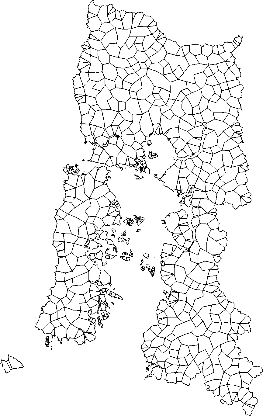
Figure 24: Los Lagos Region, Chile. The .poly file contains $294540$ vertices and $294242$ segments. The initial triangulation was generated using Triangle triangle2d with maximum area size of $100000000$ as option. The resulting triangulation was a conforming Delaunay triangulation with $309264$ vertices, $309305$ triangles and $618272$ edges. The final Polylla mesh contains $309264$ vertices, $12578$ polygons and $321534$ edges

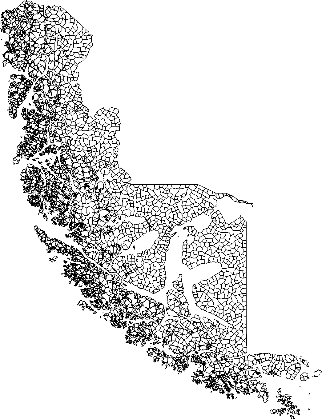
Figure 25: Magallanes Region, Chile. The .poly file contains $1130733$ vertices and $1130752$ segments. The initial triangulation was generated using Triangle triangle2d with maximum area size of $100000000$ as option. The resulting conforming Delaunay triangulation contains $1148594$ vertices, $1182133$ triangles and $2324968$ edges. The final Polylla mesh contains $1148594$ vertices, $45300$ polygons and $1186451$ edges.

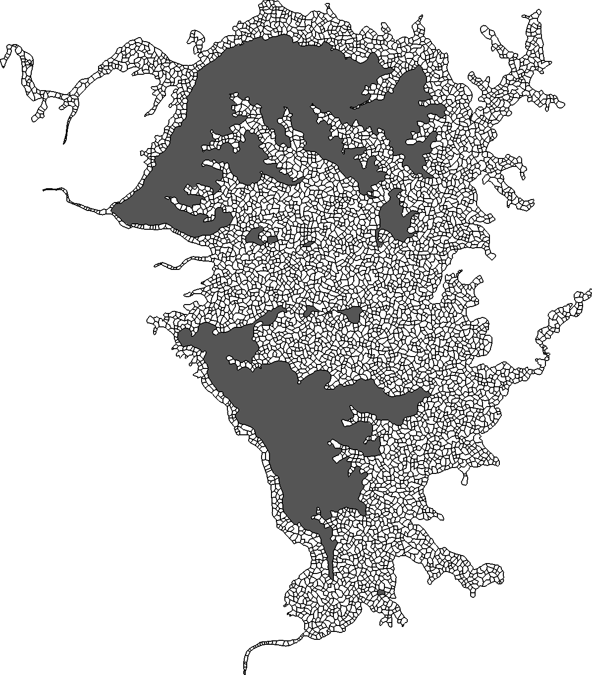
Figure 26: Budi Lake, Araucanía Region, Chile. The .poly file contains $5794$ vertices, $5794$ constrained edges and $10$ holes. The initial triangulation was generated using Triangle triangle2d with maximum area size of $10000$ as option. The resulting conforming Delaunay triangulation contains $12608$ vertices, $19406$ triangles and $32023$ edges. The final Polylla mesh contains $12608$ vertices, $5169$ polygons, $17768$ edges and $10$ holes (Islands of the lake). Grey polygons are holes.

References

- \bibcommenthead
- (1) Beirão da Veiga, L., Brezzi, F., Cangiani, A., Manzini, G., Marini, L., Russo, A.: Basic principles of virtual element methods. Mathematical Models and Methods in Applied Sciences 23(01), 199–214 (2013)
- (2) Beirão da Veiga, L., Brezzi, F., Marini, L.D.: Virtual elements for linear elasticity problems. Siam Journal on Numerical Analysis 51(2), 794–812 (2013)
- (3) Wriggers, P., Aldakheel, F., Hudobivnik, B.: Application of the virtual element method in mechanics. Technical report, Report number: ISSN 2196-3789. Leibniz Universität Hannover (January 2019)
- (4) Rivara, M.C.: New longest-edge algorithms for the refinement and/or improvement of unstructured triangulations. Int. Jour. for Num. Meth. in Eng. 40, 3313–3324 (1997)
- (5) Schlömer, N.: pygalmesh: Python Interface for CGAL’s Meshing Tools. https://doi.org/10.5281/zenodo.5564818. https://github.com/nschloe/pygalmesh
- (6) Huisman, O., de By, R.: Principles of Geographic Information Systems : an Introductory Textbook, p. 258 (2009)
- (7) Johnson, A.E., Hebert, M.: Control of polygonal mesh resolution for 3-d computer vision. Graphical Models and Image Processing 60(4), 261–285 (1998). https://doi.org/10.1006/gmip.1998.0474
- (8) Ho-Le, K.: Finite element mesh generation methods: a review and classification. Computer-Aided Design 20(1), 27–38 (1988)
- (9) Cheng, S.-W., Dey, T.K., Shewchuk, J., Sahni, S.: Delaunay Mesh Generation. CRC Press Boca Raton, FL, ??? (2013)
- (10) Yan, D.-M., Wang, W., Lévy, B., Liu, Y.: Efficient computation of clipped Voronoi diagram for mesh generation. Computer-Aided Design (2011). https://doi.org/%****␣sn-article.bbl␣Line␣175␣****10.1016/j.cad.2011.09.004
- (11) Yan, D.-M., Wang, K., Levy, B., Alonso, L.: Computing 2d periodic centroidal voronoi tessellation. In: 2011 Eighth International Symposium on Voronoi Diagrams in Science and Engineering, pp. 177–184 (2011). https://doi.org/10.1109/ISVD.2011.31
- (12) Talischi, C., Paulino, G., Pereira, A., Menezes, I.: Polymesher: A general-purpose mesh generator for polygonal elements written in matlab. Structural and Multidisciplinary Optimization 45(3), 309–328 (2012)
- (13) Löhner, R.: Progress in grid generation via the advancing front technique. Engineering with computers 12(3-4), 186–210 (1996)
- (14) Schöberl, J.: Netgen an advancing front 2d/3d-mesh generator based on abstract rules. Computing and Visualization in Science 1, 41–52 (1997)
- (15) Bern, M., Eppstein, D., Gilbert, J.: Provably good mesh generation. Journal of Computer and System Sciences 48(3), 384–409 (1994). https://doi.org/10.1016/S0022-0000(05)80059-5
- (16) Bommes, D., Lévy, B., Pietroni, N., Puppo, E., Silva, C., Tarini, M., Zorin, D.: Quad-mesh generation and processing: A survey. In: Computer Graphics Forum, vol. 32, pp. 51–76 (2013). Wiley Online Library
- (17) Owen, S.J., Staten, M.L., Canann, S.A., Saigal, S.: Q-morph: an indirect approach to advancing front quad meshing. International journal for numerical methods in engineering 44(9), 1317–1340 (1999)
- (18) Ito, Y., Nakahashi, K.: Unstructured mesh generation for viscous flow computations. IMR 2002, 367–377 (2002)
- (19) Owen, S.J.: A survey of unstructured mesh generation technology. IMR 239, 267 (1998)
- (20) Johnen, A.: Indirect quadrangular mesh generation and validation of curved finite elements. PhD thesis, Université de Liège, Liège, Belgique (2016)
- (21) Lee, C.K., Lo, S.H.: A new scheme for the generation of a graded quadrilateral mesh. Computers & Structures 52(5), 847–857 (1994)
- (22) Remacle, J.-F., Lambrechts, J., Seny, B., Marchandise, E., Johnen, A., Geuzainet, C.: Blossom-quad: A non-uniform quadrilateral mesh generator using a minimum-cost perfect-matching algorithm. International Journal for Numerical Methods in Engineering 89(9), 1102–1119 (2012)
- (23) Merhof, D., Grosso, R., Tremel, U., Greiner, G.: Anisotropic quadrilateral mesh generation : an indirect approach. Advances in Engineering Software 38(11/12), 860–867 (2007)
- (24) Shewchuk, J.R.: Triangle: Engineering a 2d quality mesh generator and delaunay triangulator. In: Lin, M.C., Manocha, D. (eds.) Applied Computational Geometry Towards Geometric Engineering, pp. 203–222. Springer, Berlin, Heidelberg (1996)
- (25) Si, H.: An Introduction to Unstructured Mesh Generation Methods and Softwares for Scientific Computing. Course. 2019 International Summer School in Beihang University (2019)
- (26) Barber, C.B., Dobkin, D.P., Huhdanpaa, H.: The quickhull algorithm for convex hulls. Acm Transactions on Mathematical Software 22(4), 469–483 (1996)
- (27) Yvinec, M.: 2D triangulations. In: CGAL User and Reference Manual, 5.3.1 edn. CGAL Editorial Board, CGAL project (2021). {}{}}{https://doc.cgal.org/5.3.1/Manual/packages.html#PkgTriangulation2}{cmtt}
- (28) Chew, L.P.: Constrained delaunay triangulation. In: Algorithmica, vol. 4, pp. 97–108 (1994)
- (29) Canann, S.A., Tristano, J.R., Staten, M.L.: An aproach to combined laplacian and optimization-based smoothing for triangular, quadrilateral and quad-dominant meshes. In: 7th International Meshing Roundtable, pp. 479–494 (1998)
- (30) Lee, K.-Y., Kim, I.-I., Cho, D.-Y., Kim, T.-w.: An algorithm for automatic 2d quadrilateral mesh generation with line constraints. Computer-Aided Design 35(12), 1055–1068 (2003)
- (31) Owen, S.J., Staten, M.L., Canann, S.A., Saigal, S.: Advancing front quadrilateral meshing using triangle transformations. In: Proceedings, 7th International Meshing Roundtable 98, pp. 409–428 (1998)
- (32) Jaillet, F., Lobos, C.: Fast Quadtree/Octree adaptive meshing and re-meshing with linear mixed elements. Engineering with Computers, 1435–5663 (2021)
- (33) Perumal, L.: A brief review on polygonal/polyhedral finite element methods. Mathematical Problems in Engineering 2018, 1–22 (2018)
- (34) Chi, H., Talischi, C., Lopez-Pamies, O., Paulino, G.: Polygonal finite elements for finite elasticity. International Journal for Numerical Methods in Engineering 101, 305–328 (2015)
- (35) Yan, D.-M., Wang, W., Lévy, B., Liu, Y.: Efficient computation of 3d clipped voronoi diagram. In: GMP, pp. 269–282 (2010)
- (36) Ebeida, M.S., Mitchell, S.A.: Uniform random Voronoi meshes. In: Quadros, W.R. (ed.) Proceedings of the 20th International Meshing Roundtable, pp. 273–290. Springer, Berlin, Heidelberg (2012)
- (37) Sieger, D., Alliez, P., Botsch, M.: Optimizing voronoi diagrams for polygonal finite element computations. In: Proceedings of the 19th International Meshing Roundtable, IMR 2010, October 3-6, 2010, Chattanooga, Tennessee, USA, pp. 335–350 (2010)
- (38) Wachspress, E.L.: A Rational Finite Element Basis. Mathematics in science and engineering. Academic Press, USA (1975)
- (39) Sukumar, N., Malsch, E.A.: Recent advances in the construction of polygonal finite element interpolants. Archives of Computational Methods in Engineering 13(1), 129–163 (2006)
- (40) Tabarraei, A., Sukumar, N.: Extended finite element method on polygonal and quadtree meshes. Computer Methods in Applied Mechanics and Engineering 197(5), 425–438 (2008)
- (41) Beirão da Veiga, L., Lovadina, C., Mora, D.: A virtual element method for elastic and inelastic problems on polytope meshes. Computer Methods in Applied Mechanics and Engineering 295, 327–346 (2015)
- (42) Cáceres, E., Gatica, G.N., Sequeira, F.A.: A mixed virtual element method for the brinkman problem. Mathematical Models and Methods in Applied Sciences 27(04), 707–743 (2017)
- (43) Cáceres, E., Gatica, G.N., Sequeira, F.A.: A mixed virtual element method for quasi-newtonian stokes flows. SIAM Journal on Numerical Analysis 56(1), 317–343 (2018)
- (44) Benedetto, M.F., Berrone, S., Pieraccini, S., Scialò, S.: The virtual element method for discrete fracture network simulations. Computer Methods in Applied Mechanics and Engineering 280, 135–156 (2014)
- (45) Wriggers, P., Reddy, B.D., Rust, W.T., Hudobivnik, B.: Efficient virtual element formulations for compressible and incompressible finite deformations. Computational Mechanics 60, 253–268 (2017)
- (46) Wriggers, P., Hudobivnik, B.: A low order virtual element formulation for finite elasto-plastic deformations. Computer Methods in Applied Mechanics 327, 459–477 (2017)
- (47) Hussein, A., Aldakheel, F., Hudobivnik, B., Wriggers, P., Guidault, P.-A., Allix, O.: A computational framework for brittle crack-propagation based on efficient virtual element method. Finite Elements in Analysis and Design 159, 15–32 (2019)
- (48) Aldakheel, F., Hudobivnik, B., Wriggers, P.: Virtual element formulation for phase-field modeling of ductile fracture. International Journal for Multiscale Computational Engineering 17(2), 181–200 (2019)
- (49) Park, K., Chi, H., Paulino, G.H.: On nonconvex meshes for elastodynamics using virtual element methods with explicit time integration. Computer Methods in Applied Mechanics and Engineering 356, 669–684 (2019)
- (50) Chi, H., da Veiga, L.B., Paulino, G.H.: Some basic formulations of the virtual element method (vem) for finite deformations. Computer Methods in Applied Mechanics and Engineering 318, 148–192 (2017)
- (51) Torres, J., Hitschfeld, N., Ruiz, R.O., Ortiz-Bernardin, A.: Convex polygon packing based meshing algorithm for modeling of rock and porous media. In: Krzhizhanovskaya, V.V., Závodszky, G., Lees, M.H., Dongarra, J.J., Sloot, P.M.A., Brissos, S., Teixeira, J. (eds.) Computational Science – ICCS 2020, pp. 257–269. Springer, Cham (2020)
- (52) Alonso, R., Ojeda, J., Hitschfeld, N., Hervías, C., Campusano, L.E.: Delaunay based algorithm for finding polygonal voids in planar point sets. Astronomy and Computing 22, 48–62 (2018)
- (53) Ojeda, J., Alonso, R., Hitschfeld-Kahler, N.: A new algorithm for finding polygonal voids in delaunay triangulations and its parallelization. In: The 34th European Workshop on Computational Geometry, EuroCG, pp. 349–354 (2018)
- (54) Hervías, C., Hitschfeld-Kahler, N., Campusano, L.E., Font, G.: On finding large polygonal voids using Delaunay triangulation: The case of planar point sets. In: Proceedings of the 22nd International Meshing Roundtable, pp. 275–292 (2013)
- (55) De Floriani, L., Kobbelt, L., Puppo, E.: A survey on data structures for level-of-detail models. In: Dodgson, N.A., Floater, M.S., Sabin, M.A. (eds.) Advances in Multiresolution for Geometric Modelling, pp. 49–74. Springer, Berlin, Heidelberg (2005)
- (56) Boissonnat, J.-D., Devillers, O., Pion, S., Teillaud, M., Yvinec, M.: Triangulations in cgal. Computational Geometry 22(1), 5–19 (2002). https://doi.org/10.1016/S0925-7721(01)00054-2. 16th ACM Symposium on Computational Geometry
- (57) Turner, R.: Deldir: Delaunay Triangulation and Dirichlet (Voronoi) Tessellation. (2021). R package version 0.2-10. https://CRAN.R-project.org/package=deldir
- (58) Austral University of Chile: Patagón Supercomputer (2021). https://patagon.uach.cl
- (59) Karavelas, M.: 2D voronoi diagram adaptor. In: CGAL User and Reference Manual, 5.3.1 edn. CGAL Editorial Board, CGAL project (2021). https://doc.cgal.org/5.3.1/Manual/packages.html#PkgVoronoiDiagram2
- (60) Ortiz-Bernardin, A., Álvarez, C., Hitschfeld-Kahler, N., Russo, A., Silva-Valenzuela, R., Olate-Sanzana, E.: Veamy: an extensible object-oriented C++ library for the virtual element method. Numerical Algorithms 82(4), 1–32 (2019)
- (61) Mitchell, W.F.: A collection of 2d elliptic problems for testing adaptive grid refinement algorithms. Applied Mathematics and Computation 220, 350–364 (2013)