Monitoring inner regions in the RY Tau jet

Abstract

We present multi-epoch observations of the RY Tau jet for H$\alpha$ and [Fe II] 1.644 µm emission lines obtained with Subaru/SCExAO+VAMPIRES, Gemini/NIFS, and Keck/OSIRIS in 2019–2021. These data show a series of four knots within 1$\arcsec$ consistent with the proper motion of $\sim$0$\farcs$3 yr^-1, analogous to the jets associated with another few active T-Tauri stars. However, the spatial intervals between the knots suggest the time intervals of the ejections of about 1.2, 0.7, and 0.7 years, significantly shorter than those estimated for the other stars. These H$\alpha$ images contrast with the archival VLT/SPHERE/ZIMPOL observations from 2015, which showed only a single knot-like feature at $\sim 0\farcs 25$. The difference between the 2015 and 2019–2021 epochs suggests an irregular ejection interval within the six-year range. Such variations of the jet ejection may be related to a short-term ($<$1 year) variability of the mass accretion rate. We compared the peaks of the H$\alpha$ emissions with the ZIMPOL data taken in 2015, showing the brighter profile at the base ($<0\farcs 3$) than the 2020–2021 VAMPIRES profiles due to time-variable mass ejection rates or the heating-cooling balance in the jet. The observed jet knot structures may be alternatively attributed to stationary shocks, but a higher angular resolution is required to confirm its detailed origin.

monthyearday []

1 Introduction

Young stellar objects of various masses and at various evolutionary stages are known to host collimated jets. Those at the base, within 100 au of the star (corresponding to $\sim$$1\arcsec$ for the nearest star forming regions), have drawn particular attentions over many years to understand the jet launching mechanism and its physical link with mass accretion (e.g. Cabrit et al., 1990; Hartigan et al., 1995; Takami et al., 2020). Unlike more extended parts of the jet, the structures at the base are very compact: in many cases, we have been able to observe them just as chains of knotty structures, as probable signatures of time variable mass ejection, even with the best angular resolutions available (e.g. Ray et al., 2007; Frank et al., 2014, for reviews). Information about more detailed structures in these jets is highly desired to understand the key issues described above.

Furthermore, observations of emission lines at a variety of excitation conditions have been tremendously useful to understand the physical conditions in the jet. Such studies have been made for extended energetic jets ($\gg$1000 au from the star) called Herbig-Haro objects (see Hartigan et al., 2000; Reipurth & Bally, 2001, for reviews). This contrasts to the observations of jets at the base, which have been made for most cases using only low-excitation forbidden lines like [O I], [S II] and [Fe II] (see Eisloffel et al., 2000; Ray et al., 2007; Frank et al., 2014, for reviews).

State-of-the-art adaptive optics (AO) at optical wavelengths will yield a breakthrough in the studies of jets at the base. This technique provides an angular resolution smaller than 0$\farcs$1 on a 8-10 m telescope, about 2-3 times better than most of the seeing-limited observations to date. These instruments enable us to observe H$\alpha$ emission, one of the brightest emission lines associated with the Herbig-Haro objects. This emission line, observed at the base of only a small number of young stars (e.g. Bacciotti et al., 2000; Takami et al., 2001; Ray et al., 2007), requires an excitation energy significantly larger than the low-excitation needed to trigger the forbidden lines mentioned above, therefore useful for tracing shocks with significantly higher temperatures and/or higher shock velocities etc.

Here we present multi-epoch H$\alpha$ imaging observations of RY Tau at an extremely high angular resolution (50-60 mas), complemented by near-infrared [Fe II] observations. RY Tau is a T Tauri Star (TTS) embedded in an envelope and protoplanetary disk in the Taurus star forming region (Kenyon et al., 2008). The previous measurements of the distance have suggested different values, which makes it hard to accurately characterize the stellar parameters. Garufi et al. (2019) updated the stellar parameters in detail ($T_{\rm eff}$=5750 K, $L_{\star}=6.3^{+9.1}_{-3.2}\ L_{\odot}$, $M_{\star}=1.8\ M_{\odot}$, and age $\sim 1.8$ Myr) using Gaia DR2-based distance (133 pc; Gaia Collaboration et al., 2018). Among pre-main sequence stars, RY Tau hosts one of the most active and best studied jets as highly excited lines such as H$\alpha$ (St-Onge & Bastien, 2008; Garufi et al., 2019), He I (Garufi et al., 2019), and CIV (Skinner et al., 2018) have been observed as well as frequently-used forbidden lines such as optical [O I], [S II], [N II] and near-infrared [Fe II] (Agra-Amboage et al., 2009; Garufi et al., 2019).

In this paper, we describe the H$\alpha$ and [Fe II] data used in this study in Section 2 and their results in Section 3. Section 4 discusses substructures in the jet and its movement, as well as the ejection mechanisms.

2 Observations and Data Reduction

Table 1: Observing Logs

Instrument, Line	Date [UT]	$t_{\rm int}$ [sec]	$N_{\rm exp}$	FWHM [mas]	Modea	Field rotation
VLT/SPHERE/ZIMPOL, H$\alpha$	2015 Nov 8	118	24	50	SDI	…
Geimini/NIFS, [Fe II]	2019 Oct 25	15	108	126	SDI	…
Subaru/SCExAO+VAMPIRESb, H$\alpha$	2020 Jan 31	1	2497	60	ADI+SDI	59∘
Keck/OSIRIS, [Fe II]	2021 Feb 03	20	46	50-100c	SDI	…
Subaru/SCExAO+VAMPIRESb,d, H$\alpha$	2021 Sep 11	0.5	6748	64	ADI+double-SDI	63∘

Note. — ^a See Section 2 for the detailed explanations of each reduction method.

^b The VAMPIRES data format is a cube consisting of a 2-dimension image and exposure. The number of exposures ($N_{\rm exp}$) corresponds to the total exposures but in practice we selected 40-50% percentile in each cube before post-processing. FWHM is measured after the frame selection.

^c See text for details.

^d $N_{\rm exp}$ corresponds to the total exposures in State 1 and 2 (see Section 2.1).

2.1 H$\alpha$ Emission Line

We observed RY Tau with Subaru/SCExAO+VAMPIRES on 2020 January 31 UT (engineering run) and on 2021 September 11 (PI: Taichi Uyama, as a backup target). The detailed exposure settings are presented in Table 1. VAMPIRES enables simultaneous imaging with the narrow-band H$\alpha$ filter ($\lambda_{\rm c}=656.3$ nm, $\Delta\lambda=1.0$ nm) and the adjacent continuum filter ($\lambda_{\rm c}=647.68$ nm, $\Delta\lambda=2.05$ nm) with two detectors. To mitigate the aberration between these detectors we utilize a double-differential imaging technique by switching the filters (see Norris et al., 2015; Uyama et al., 2020, for the schematic). We set two states where H$\alpha$ and continuum data are taken at the different detectors (State 1: continuum - camera 1, H$\alpha$ - camera 2. State 2 is the other way around). This will help to better subtract continuum components from the H$\alpha$ image and we call this subtraction method as ‘double-SDI’ (see below and Uyama et al., 2020, for the detailed descriptions). However, we note that the first VAMPIRES data set, which was obtained for science verification, did not utilize the double-differential imaging technique.

The VAMPIRES data format is a cube consisting of short exposures ($t_{\rm int}$). As for data reduction, we first subtract dark from each exposure and conduct PSF fitting by 2D-Gaussian of continuum PSFs for frame selection. We then selected the ‘best’ AO-corrected exposures in each cube based on the peak intensity of the stellar PSF that reflects efficiency of AO correction. We adopted the 40% and 50% percentiles, for the first and second data sets respectively, among the fitted PSF peaks as the selection criteria. We then combined the selected exposures into an image after aligning the centroid of the PSFs (see Figure 2 in Uyama et al., 2020). To remove stellar halo and to detect the H$\alpha$ jet feature we applied angular differential imaging (ADI; Marois et al., 2006) and spectral differential imaging (SDI; Smith, 1987).

The preliminary ADI+SDI result for the first VAMPIRES data set is presented in Uyama et al. (2020), and we updated the post-processing, particularly SDI reduction, as mentioned below. 1) We used the continuum data as a PSF reference for SDI. To prepare SDI reduction we took into account the central star’s accretion, difference of the filter transmissions, and the systematic difference of the VAMPIRES detectors. We calculated a scaling factor by comparing photometry (aperture radius = 10$\times$FWHM) of the central star’s PSF at each filter. This scaling factor was multiplied to the continuum data before ADI reduction. 2) We applied ADI reduction to both of the H$\alpha$ and continuum data utilizing pyklip algorithms (Wang et al., 2015), which produces the most-likely reference PSF for the target PSF by Karhunen-Loève Image Projection (KLIP: Soummer et al., 2012). Here we do not conduct aggressive PSF subtraction so that we can avoid severe attenuation and distortion of the jet features. We adopted Karhunen-Loève mode (KL)=1 and minrot=10 deg for the first VAMPIRES data set and KL=3 and minrot=10 deg for the second data set. A larger number of KL allows aggressive speckle suppression while it causes self-subtraction. The minrot parameter assumes a frame-to-frame rotation of astrophysical objects and is critical to building PSF reference libraries. For example, a small minrot value takes nearby pixels of the object into reference PSFs and can cause severe self-subtraction. Note that this parameter does not correspond to the practical frame-to-frame parallactic angle change. We experimented injection test by burying fake point sources at other position angles of the jet feature and confirmed that these pyKLIP settings caused a typical flux loss of $<10\%$ at $\rho>200$ mas and $\sim 10-20\%$ between the inner working angle ($\sim 100$ mas) and $\rho\geq 200$ mas. 3) After the ADI reduction we conducted SDI reduction to the ADI residuals (ADI+SDI) by subtracting the ADI residual image of the scaled continuum data from that of the H$\alpha$ data.

For the VAMPIRES data set taken in 2021, we obtained two states for double-differential imaging. After performing ADI+SDI reduction in each state we applied double-differential imaging to mitigate the aberrations (ADI+double-SDI).

Finally, we compared the count rate of the unsaturated PSF within an aperture of radius $10\times$FWHM with stellar flux to obtain the count-to-flux conversion factor. We utilized the central star’s $R$-band magnitude as a photometric reference because we did not observe photometric standard stars. To take into account variability we referred to the American Association of Variable Star Observers (AAVSO). AAVSO did not record the $R$-band magnitude around the VAMPIRES second observing night but the $V$-band magnitude on the nearest date to the second night (September 4 2021) is same as the first night, so we adopted the stellar flux to be 4.3$\times 10^{-9}$ erg s^-1cm^-2µm^-1 at 650 nm on both the first and second nights. We then converted the post-processed images into the surface brightness H$\alpha$ map.

We also re-reduced the archival VLT/SPHERE/ZIMPOL H$\alpha$ data, which are originally presented in Garufi et al. (2019). The data from both the B_Ha ($\lambda_{\rm c}=655.6$ nm, $\Delta\lambda=5.35$ nm) and Cnt_Ha ($\lambda_{\rm c}=644.9$ nm, $\Delta\lambda=3.83$ nm) filters were reduced with the ZIMPOL pipeline, which rescales the pixels onto a square grid with pixel scale 3.6 mas/pixel and takes care of bias and flat-field corrections. Subsequently, we used PynPoint (Stolker et al., 2019) to align images fitting a 2D-Gaussian profile to the stellar PSF and to shift the images using spline interpolation. The continuum images were then stretched in the radial direction by the ratio of the filter central wavelengths to align the speckle patterns. Furthermore, they were normalized to the simultaneous H$\alpha$ frame to correct for different band-passes using the counts in an aperture of radius 10$\times$FWHM. At this point, the SDI step could be performed, and we subtracted the continuum images from the H$\alpha$ frames and median combined the residuals, revealing the jets shown in Figure 1. We note that SDI resulted in slight negative sky background and we corrected for it by subtracting the median value of the northern sky area when reporting the results in the following sections. Finally we converted the SDI result into the surface brightness map as we did in the VAMPIRES data sets. For the ZIMPOL data we followed the prescriptions from Cugno et al. (2019) (see Section 4.1.4 in the literature for detail) to estimate the flux in both the continuum ($F_{\mathrm{Cnt\_Ha}}=3.55\pm 0.11\,\times 10^{-9}$ erg s^-1cm^-2µm^-1) and broad H$\alpha$ ($F_{\mathrm{B\_Ha}}=4.09\pm 0.32\times 10^{-9}$ erg s^-1cm^-2µm^-1) filters. Briefly, the count rate was estimated in apertures of radius $1\farcs 5$ and then converted to physical fluxes using the zero points of the filters estimated in Schmid et al. (2017).

2.2 [Fe II] 1.64-µm Forbidden Line

The AO-fed integral field spectroscopic observations of the [Fe II] 1.644 $\micron$ line were conducted on 2019 October 25 and 2021 February 3, using NIFS at the Gemini North Telescope (McGregor et al., 2003) and OSIRIS at Keck I Telescope (Larkin et al., 2006; Mieda et al., 2014), respectively, as a part of a long-term monitoring program for a few active pre-main sequence stars (Takami et al., 2020, Takami et al., in preparation). Use of the $H$ and Hn3 gratings with these instruments yielded a spectral resolution $R$$\sim$5500 ($\Delta v$=55 km s^-1) and $R$$\sim$3800 ($\Delta v$=80 km s^-1) at 1.5-1.8 and 1.59-1.67 µm, respectively. These spectral resolutions are optimal to observe the emission lines with high signal-to-noise without resolving their internal kinematics.

The Gemini data were obtained for a 3″$\times$3″filed of view (FoV) through an image slicer with the spatial sampling of 0$\farcs$1$\times$0$\farcs$04 along and across the slices, respectively. The Keck data cubes were obtained for a 2$\farcs$4$\times$3$\farcs$2 FoV through a lenslet array with a 0$\farcs$05 spatial sampling. The exposures were made with object-sky-object sequences. The star was placed near the edge of each FoV to cover the (blueshifted) jet with a large spatial area.

Data were reduced using the pipelines provided by the observatories, and software we developed using PyRAF (Science Software Branch at STScI, 2012), numpy (Harris et al., 2020), scipy (Virtanen et al., 2020) and astropy (Astropy Collaboration et al., 2013, 2018) on python. For the Gemini data, we used the Gemini IRAF package for sky subtraction, flat-fielding, the first stage of bad pixel removals, 2 to 3 dimensional transformation of the spectral data, and wavelength calibration. We then used our own software for stacking data cubes for each date, telluric correction, flux calibration, extraction of the cube for the target emission line, additional removal of bad pixels, and continuum subtraction. We have also corrected a flux loss with the PSF halo, as the jet structures we are interested in are significantly smaller than the PSF halo ($>$0$\farcs$5). We have used identical processes for the Keck data but data stacking was made using the observatory pipeline. We then integrated the intensity over the velocity range of the emission line to obtain the final images.

For the Gemini data we measured an angular resolution of 0$\farcs$12 using the target star in the stacked cube. The target star was saturated in the Keck data, and we estimated an angular resolution of 0$\farcs$05-0$\farcs$1 using the snapshots for target acquisition for the target and a spectroscopic standard. The extremely bright stellar continuum compared with line emission causes artifacts due to imperfect continuum subtraction, making the image unreliable within 0$\farcs$2 of the star.

3 Results

Figure 1 shows the images of the H$\alpha$ jets for three epochs. To increase the apparent signal-to-noise, we convolved each of the VAMPIRES and ZIMPOL images using a 2D-Gaussian ($\sigma=20$ mas). The FWHM of the PSFs after convolutions increased by $\sim 5\%$ from the original unsaturated PSFs. As a result, the emission was observed for all the epochs with signal-to-noise ratio (SNR) $\gtrsim 4$ for the first VAMPIRES data taken in 2020 January and SNR $\gtrsim 5$ for the ZIMPOL data and the second VAMPIRES data taken in 2021 September, respectively, at the spine of the jet. Among three epochs, the ZIMPOL data obtained in 2015 achieved the highest SNR probably thanks to the best AO correction and the brightest H$\alpha$ signal (see Section 4). The second VAMPIRES data obtained in 2021 achieved a better SNR than the first VAMPIRES data obtained in 2020 thanks to the double-SDI reduction.

The H$\alpha$ image in each epoch shows a series of knots at 0$\farcs$15-0$\farcs$75 (corresponding to the projected distance of 20-100 au) from the star. The jet structures are different between three epochs, indicative of time variation over six years. Note that the jet features in the VAMPIRES data may be biased in some extent because the jet feature is extended and there could happen a self-subtraction effect though we adopted the non-aggressive ADI parameters as mentioned in Section 2.1. The position angle of the jet is roughly measured at $293^{\circ}$ by eye, which is consistent with previous measurements (Pinilla et al., 2018; Garufi et al., 2019), and the latest VAMPIRES data show a curved shape and this feature is possibly connected to the wiggling feature mentioned in Garufi et al. (2019).

Figure 2 shows the images of the [Fe II] jet, which also consists of a series of knots. As seen Figures 1 and 2, our H$\alpha$ images appear to show finer structures in the jet probably due to higher angular resolutions. We measure the radial velocity of the jet of $-60$ to $-80$ km s^-1 in the [Fe II] emission (with an uncertainty of about $\pm$10 km s^-1), similar to that measured in the optical [O I] emission in the past (Agra-Amboage et al., 2009).

To investigate proper motions of the jet knots, we place the H$\alpha$ and [Fe II] images in 2019–2021 in Figure 3, taking into account the time intervals of the observations. This figure shows the presence of three or probably four knots and connecting each knot is consistent with a proper motion of $\sim$0$\farcs$3 yr^-1. The proper motion would correspond to a tangential velocity $(V_{\rm T})\sim 200\ {\rm km\ s^{-1}}$. St-Onge & Bastien (2008) monitored the RY Tau jet at separations $>1\arcsec$ between 1998 and 2004 and measured the tangential velocity as 165 km s^-1, and Garufi et al. (2019) suggested $V_{\rm T}\sim$100 km s^-1 at separations $<4\arcsec$ and $\sim 300$ km s^-1 at 5$\arcsec$. The derived value from our observations is roughly consistent with these previous studies and favors a prediction about the tangential velocity from the blue-shifted radial velocity of the jet (Skinner et al., 2018). Combining $V_{\rm T}\sim 200\ {\rm km\ s^{-1}}$ with the radial velocity measurements from our [Fe II] observations, we estimate the jet inclination at $\sim 70^{\circ}$, which is consistent with Agra-Amboage et al. (2009). The detailed proper motion and inclination measurements will be presented in the long-term monitoring project paper (Takami et al. in prep).

In Figure 3 we mark three knots as A-C and a probable new knot seen at the base of the latest H$\alpha$ image as D (see Section 4 for the detailed discussions). We note that the H$\alpha$ and forbidden lines reflect different velocity components in terms of quenching and excitation (see e.g. Bacciotti et al., 2000; Garufi et al., 2019, for details) and that H$\alpha$ is more sensitive to the higher velocity than [Fe II]. Thus, there are possibly slight differences between the peaks of the knots in the H$\alpha$ and [Fe II] images.

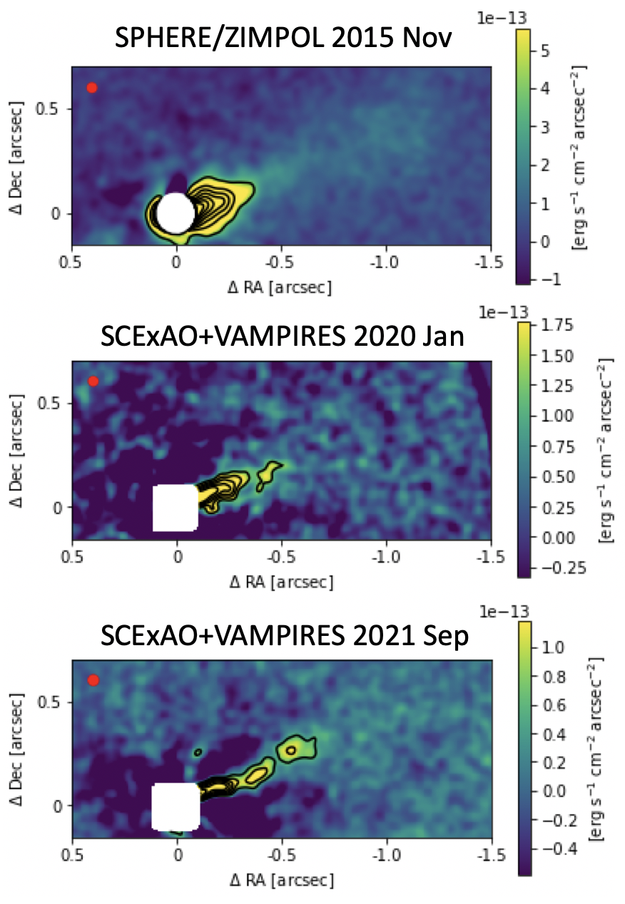
Figure 1: Comparison of the VLT/ZIMPOL H$\alpha$ data taken in 2015 November (top) and the Subaru/VAMPIRES H$\alpha$ data taken in 2020 January (middle) and 2021 September (bottom). The images are convolved by 2D-Gaussian (see text) and the color scale and contours are arbitrarily set to clearly show the jet feature. North is up and East is left. The typical FWHM of the observation after convolution is indicated by a red circle at top left of each panel. In the ZIMPOL data we put a $0\farcs 1$ mask because the continuum subtraction did not work well. For the VAMPIRES data sets the central star is masked by the post-processing algorithms.

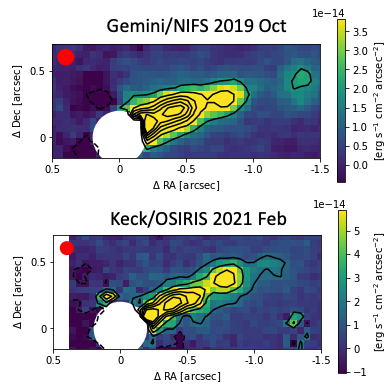
Figure 2: Same as Figure 1 but for the Gemini/NIFS [Fe II] data taken in 2019 October (top) and the Keck/OSIRIS [Fe II] data taken in 2021 February (bottom). We put a $0\farcs 2$ mask in each panel because the continuum subtraction did not work well.

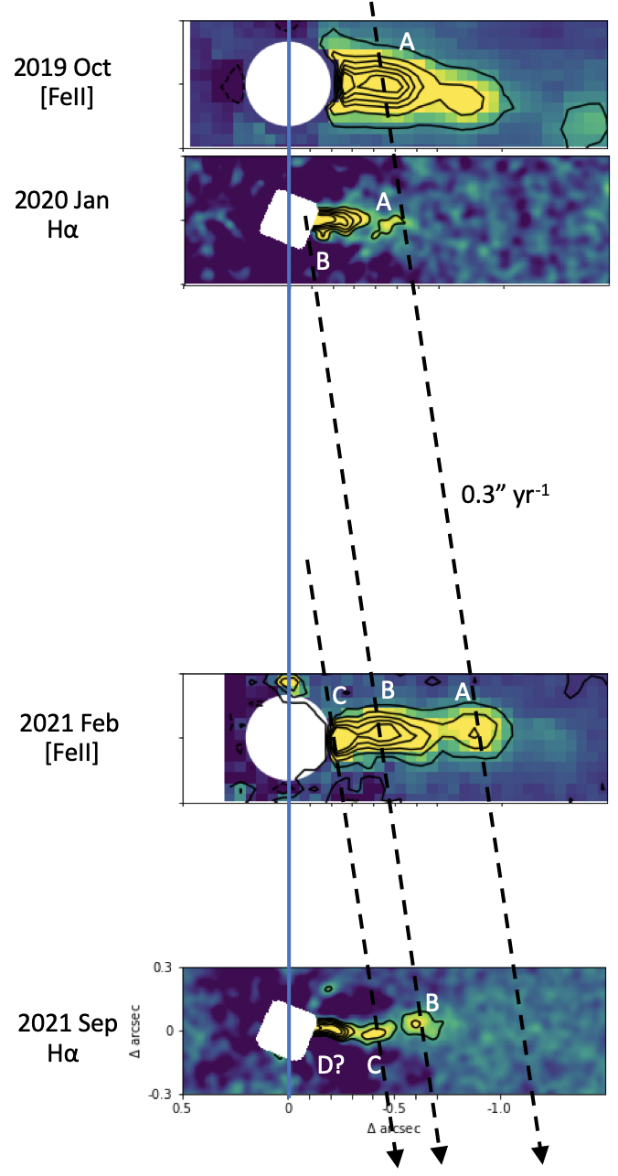
Figure 3: A year-scale monitoring result of the RY Tau jet. For the clarity we rotated all the field of views by 23^∘ to horizontally align them. The vertical separations between the panels correspond to the time between the epochs. The central star’s location is indicated by a dark-blue vertical line. The three dashed lines correspond to roughly-estimated proper motions of the knots A, B, and C ($\sim 0\farcs 3/{\rm yr}$).

Figure 4 shows the traced peak of the H$\alpha$ feature as a surface brightness function of separation. We divided the jet feature along separation into several areas by a step of FWHM and adopted the peak pixel as surface brightness at the given separation. The H$\alpha$ jet observed in 2015 shows brighter surface brightness than that observed between 2020–2021.

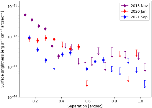
Figure 4: Radial profiles of H$\alpha$ surface brightness from the ZIMPOL (taken in 2015 November) and VAMPIRES data sets (taken in 2020 January and 2021 September). The circle and arrow symbols indicate SNR $\geq 4$ and $<4$ respectively. The SNR is calculated with the pyklip cross-correlation functions after 2D-Gaussian convolution as mentioned in Section 3. We do not correct flux loss and distortion caused by the post-processing because we adopted the non-aggressive PSF subtraction (see text) and in fact it is difficult to model the H$\alpha$ jet.

4 Discussion

As shown above, our multi-epoch observations of the jet knots are consistent with the presence of proper motions of $\sim$0$\farcs$3 yr^-1. This interpretation is consistent with similar observations for another two TTSs at similar distances ($d$$\sim$140 pc). Takami et al. (2020) presented seven epochs of jet knot imaging in the [Fe II] 1.644 $\micron$ emission at $>$0$\farcs$2 from RW Aur A, and attributed them to moving knots with proper motions of 0$\farcs$2-0$\farcs$3 yr^-1. White et al. (2014) combined three epochs of similar observations with those in literature, and identified moving knots at $\gtrsim$0$\farcs$4 from DG Tau with similar proper motions.

As described in the previous section, the interpretation of moving knots is also consistent with the proper motions of the knots measured downstream ($>$1″) for the same star. Furthermore, with an estimate of the proper motions of $\sim$0$\farcs$3, we have derived the jet inclination of $\sim$70°, consistent with the previous analysis by another group. Although the present data set does not allow us to accurately estimate the uncertainties of the proper motions, Figure 3 suggests that it is significantly smaller than a factor of 2. We believe that this uncertainty does not affect our discussion below.

The X-ray observations of jets from some protostars and young stars indicate the presence of the following two components: (1) an inner stationary component probably related to jet/outflow collimation; and (2) the outer components with proper motions, which are probably related to working surfaces where the shocks travel through the jet (e.g., Schneider & Schmitt, 2008; Schneider et al., 2011). Such jets include one associated with DG Tau. The X-ray and near-infrared observations of this jet suggested the location of the stationary component of $\sim$30 au from the star (Güdel et al., 2011; White et al., 2014). Therefore, one may alternatively attribute the observed jet knots shown in Figure 3 to stationary shocks, e.g., at 0$\farcs$2, 0$\farcs$4 and 0$\farcs$8 from the star. Our data do not exclude this possibility, however, it might yield the following puzzle: the H$\alpha$ image obtained in February 2021 shows knot B at 0$\farcs$6 from the star, but none of the images obtained in the other epochs show its counterpart.

For the rest of this section, we tentatively attribute the jet knots ABC in Figure 3 to moving knots as demonstrated. Confirmation of this interpretation requires observations of proper motions with more epochs with smaller time intervals, or those at higher angular resolutions to resolve shock structures.

To investigate the time variation over a six-year timescale we compared the ZIMPOL data taken in 2015 with the other data sets, particularly with the VAMPIRES H$\alpha$ data. In the ZIMPOL data the knot-like feature is detected at $\sim 0\farcs 25$ while the 2019–2021 data sets show three or four knots within $1\arcsec$. The difference between the 2015 and 2019-2021 observations suggests that the knot ejection interval is irregular within the six-year range.

In Figure 3, the VAMPIRES H$\alpha$ images show the intervals of the knots A-D of 0$\farcs$35, 0$\farcs$2, and 0$\farcs$2, respectively, indicative of time intervals of the ejections of about 1.2, 0.7 and 0.7 years adopting the proper motion of 0$\farcs$3 yr^-1. These intervals are significantly shorter than those measured for a few active T-Tauri jets to date such as DG Tau ($\sim 2.5-5$ yr; Pyo et al., 2003; White et al., 2014), RW Aur (irregular intervals between 3 and 20 yr; López-Martín et al., 2003; Takami et al., 2020), and XZ Tau ($\sim 5-10$ yr; Krist et al., 2008).

Such variabilities for jet ejection may be related to activities of mass accretion from the inner disk edge to the star. Theoretical studies have suggested that the jet ejection mechanism is related to accretion onto the central star (see Najita et al., 2000, for a review). Petrov et al. (1999) and Grankin et al. (2007) monitored RY Tau’s optical spectrum/flux and Chou et al. (2013) investigated mass accretion signatures such as H$\alpha$, which presented short-term variabilities ($\lesssim 1$ yr). The derived knot interval of 0.7–1.2 years from our results suggests a potential connection with these short-term variability, but we note that the 22d-period variability of H$\alpha$ and Na D absorption presented by Petrov et al. (2021) is not directly connected to the knot intervals shown in this study. Grankin et al. (2007) also presented long-term variabilities in the flux of DG Tau, RW Aur, and RY Tau, and Garufi et al. (2019) suggested a possible connection between the RY Tau jet ejection and an episodic accretion. However RY Tau does not have unique feature among these three TTS light curves except for circumstellar dust obscuration (e.g. Grankin et al., 2007; Petrov et al., 2019). Detailed investigations of the relationship between the variability and the knot ejection intervals will help to address the RY Tau jet ejection mechanism in the context of the TTS jet studies.

As shown in Section 3, the H$\alpha$ emission at the base ($<$0$\farcs$3) is brighter in 2015 than 2020–2021 by a factor of 3-6, perhaps due to different mass ejection rates or heating-cooling balance. The latter would be variable due to different shock conditions (see Ray et al., 2007, for a review) or prompt heating induced by magnetic processes at the base (Skinner et al., 2018). This issue will be discussed in a separate paper with large data sets for jet ejection and signature for mass accretion.

5 Summary

We have presented monitoring results of the RY Tau jet between 2015 and 2021 using H$\alpha$ and [Fe II] emission lines with Subaru/SCExAO+VAMPIRES, VLT/SPHERE/ZIMPOL, Gemini/NIFS, and Keck/OSIRIS. The 2019–2021 data detected a series of three or four knots within 1″consistent with the proper motion of $\sim$0$\farcs$3 yr^-1, with its uncertainty significantly less than a factor of 2. This would correspond to the tangential velocity of $\sim$200 km s^-1, and the radial velocity of $-60$ to $-80$ km s^-1. These values and the jet inclination estimated from them are consistent with the previous measurements of the RY Tau jet. The observed jet intervals between 2019 and 2021 suggest the time intervals of jet knot ejections of about 1.2, 0.7, and 0.7 years and these values are significantly shorter than other T-Tauri jets measured to date. On the other hand the 2015 data detected only one knot-like feature at $\sim 0\farcs 25$ and the difference from the 2019–2021 observations suggests the irregular ejection interval within the six-year range. Such variations of the jet ejection may be related to the short-term variability of mass accretion onto the central star. We compared the peak of the H$\alpha$ emissions and the 2015 data show the brighter profile at the base ($<0\farcs 3$) than the 2020–2021 data perhaps due to different mass ejection rates or heating-cooling balance. This degeneration will be discussed with a large data sets combining jet ejection and mass accretion measurements.

The interpretation of the moving knots within $\sim$100 au of the star is consistent with those in literature for jets associated with another few active T-Tauri stars. Even so, our results do not exclude a possibility that the observed jet knots may be alternatively attributed to stationary shocks related to outflow collimation. However, this scenario would require an explanation about a sudden emergence of one of the knots at 0$\farcs$6 from the star in the latest epoch of the observations. Throughout, a higher angular resolution is required to confirm the detailed origin of the observed jet knots.

References

- Agra-Amboage et al. (2009) Agra-Amboage, V., Dougados, C., Cabrit, S., Garcia, P. J. V., & Ferruit, P. 2009, A&A, 493, 1029, doi: 10.1051/0004-6361:200810025
- Astropy Collaboration et al. (2013) Astropy Collaboration, Robitaille, T. P., Tollerud, E. J., et al. 2013, A&A, 558, A33, doi: 10.1051/0004-6361/201322068
- Astropy Collaboration et al. (2018) Astropy Collaboration, Price-Whelan, A. M., Sipőcz, B. M., et al. 2018, AJ, 156, 123, doi: 10.3847/1538-3881/aabc4f
- Bacciotti et al. (2000) Bacciotti, F., Mundt, R., Ray, T. P., et al. 2000, ApJ, 537, L49, doi: 10.1086/312745
- Cabrit et al. (1990) Cabrit, S., Edwards, S., Strom, S. E., & Strom, K. M. 1990, ApJ, 354, 687, doi: 10.1086/168725
- Chou et al. (2013) Chou, M.-Y., Takami, M., Manset, N., et al. 2013, AJ, 145, 108, doi: 10.1088/0004-6256/145/4/108
- Cugno et al. (2019) Cugno, G., Quanz, S. P., Hunziker, S., et al. 2019, A&A, 622, A156, doi: 10.1051/0004-6361/201834170
- Eisloffel et al. (2000) Eisloffel, J., Mundt, R., Ray, T. P., & Rodriguez, L. F. 2000, in Protostars and Planets IV, ed. V. Mannings, A. P. Boss, & S. S. Russell, 815
- Frank et al. (2014) Frank, A., Ray, T. P., Cabrit, S., et al. 2014, Protostars and Planets VI, 451, doi: 10.2458/azu_uapress_9780816531240-ch020
- Gaia Collaboration et al. (2018) Gaia Collaboration, Brown, A. G. A., Vallenari, A., et al. 2018, A&A, 616, A1, doi: 10.1051/0004-6361/201833051
- Garufi et al. (2019) Garufi, A., Podio, L., Bacciotti, F., et al. 2019, A&A, 628, A68, doi: 10.1051/0004-6361/201935546
- Grankin et al. (2007) Grankin, K. N., Melnikov, S. Y., Bouvier, J., Herbst, W., & Shevchenko, V. S. 2007, A&A, 461, 183, doi: 10.1051/0004-6361:20065489
- Güdel et al. (2011) Güdel, M., Audard, M., Bacciotti, F., et al. 2011, in Astronomical Society of the Pacific Conference Series, Vol. 448, 16th Cambridge Workshop on Cool Stars, Stellar Systems, and the Sun, ed. C. Johns-Krull, M. K. Browning, & A. A. West, 617. https://arxiv.org/abs/1101.2780
- Harris et al. (2020) Harris, C. R., Millman, K. J., van der Walt, S. J., et al. 2020, Nature, 585, 357, doi: 10.1038/s41586-020-2649-2
- Hartigan et al. (2000) Hartigan, P., Bally, J., Reipurth, B., & Morse, J. A. 2000, in Protostars and Planets IV, ed. V. Mannings, A. P. Boss, & S. S. Russell, 841
- Hartigan et al. (1995) Hartigan, P., Edwards, S., & Ghandour, L. 1995, ApJ, 452, 736, doi: 10.1086/176344
- Kenyon et al. (2008) Kenyon, S. J., Gómez, M., & Whitney, B. A. 2008, in Handbook of Star Forming Regions, Volume I, The Northern Sky, ed. B. Reipurth, Vol. 4, 405
- Krist et al. (2008) Krist, J. E., Stapelfeldt, K. R., Hester, J. J., et al. 2008, AJ, 136, 1980, doi: 10.1088/0004-6256/136/5/1980
- Larkin et al. (2006) Larkin, J., Barczys, M., Krabbe, A., et al. 2006, in Society of Photo-Optical Instrumentation Engineers (SPIE) Conference Series, Vol. 6269, Society of Photo-Optical Instrumentation Engineers (SPIE) Conference Series, ed. I. S. McLean & M. Iye, 62691A, doi: 10.1117/12.672061
- López-Martín et al. (2003) López-Martín, L., Cabrit, S., & Dougados, C. 2003, A&A, 405, L1, doi: 10.1051/0004-6361:20030758
- Marois et al. (2006) Marois, C., Lafrenière, D., Doyon, R., Macintosh, B., & Nadeau, D. 2006, ApJ, 641, 556, doi: 10.1086/500401
- McGregor et al. (2003) McGregor, P. J., Hart, J., Conroy, P. G., et al. 2003, in Society of Photo-Optical Instrumentation Engineers (SPIE) Conference Series, Vol. 4841, Instrument Design and Performance for Optical/Infrared Ground-based Telescopes, ed. M. Iye & A. F. M. Moorwood, 1581–1591, doi: 10.1117/12.459448
- Mieda et al. (2014) Mieda, E., Wright, S. A., Larkin, J. E., et al. 2014, PASP, 126, 250, doi: 10.1086/675784
- Najita et al. (2000) Najita, J. R., Edwards, S., Basri, G., & Carr, J. 2000, in Protostars and Planets IV, ed. V. Mannings, A. P. Boss, & S. S. Russell, 457
- Norris et al. (2015) Norris, B., Schworer, G., Tuthill, P., et al. 2015, MNRAS, 447, 2894, doi: 10.1093/mnras/stu2529
- Petrov et al. (2021) Petrov, P. P., Romanova, M. M., Grankin, K. N., et al. 2021, MNRAS, 504, 871, doi: 10.1093/mnras/stab904
- Petrov et al. (1999) Petrov, P. P., Zajtseva, G. V., Efimov, Y. S., et al. 1999, A&A, 341, 553
- Petrov et al. (2019) Petrov, P. P., Grankin, K. N., Gameiro, J. F., et al. 2019, MNRAS, 483, 132, doi: 10.1093/mnras/sty3066
- Pinilla et al. (2018) Pinilla, P., Tazzari, M., Pascucci, I., et al. 2018, ApJ, 859, 32, doi: 10.3847/1538-4357/aabf94
- Pyo et al. (2003) Pyo, T.-S., Kobayashi, N., Hayashi, M., et al. 2003, ApJ, 590, 340, doi: 10.1086/374966
- Ray et al. (2007) Ray, T., Dougados, C., Bacciotti, F., Eislöffel, J., & Chrysostomou, A. 2007, Protostars and Planets V, 231
- Reipurth & Bally (2001) Reipurth, B., & Bally, J. 2001, ARA&A, 39, 403, doi: 10.1146/annurev.astro.39.1.403
- Schmid et al. (2017) Schmid, H. M., Bazzon, A., Milli, J., et al. 2017, A&A, 602, A53, doi: 10.1051/0004-6361/201629416
- Schneider et al. (2011) Schneider, P. C., Günther, H. M., & Schmitt, J. H. M. M. 2011, A&A, 530, A123, doi: 10.1051/0004-6361/201016305
- Schneider & Schmitt (2008) Schneider, P. C., & Schmitt, J. H. M. M. 2008, A&A, 488, L13, doi: 10.1051/0004-6361:200810261
- Science Software Branch at STScI (2012) Science Software Branch at STScI. 2012, PyRAF: Python alternative for IRAF. http://ascl.net/1207.011
- Skinner et al. (2018) Skinner, S. L., Schneider, P. C., Audard, M., & Güdel, M. 2018, ApJ, 855, 143, doi: 10.3847/1538-4357/aaab58
- Smith (1987) Smith, W. H. 1987, PASP, 99, 1344, doi: 10.1086/132124
- Soummer et al. (2012) Soummer, R., Pueyo, L., & Larkin, J. 2012, ApJ, 755, L28, doi: 10.1088/2041-8205/755/2/L28
- St-Onge & Bastien (2008) St-Onge, G., & Bastien, P. 2008, ApJ, 674, 1032, doi: 10.1086/524649
- Stolker et al. (2019) Stolker, T., Bonse, M. J., Quanz, S. P., et al. 2019, A&A, 621, A59, doi: 10.1051/0004-6361/201834136
- Takami et al. (2001) Takami, M., Bailey, J., Gledhill, T. M., Chrysostomou, A., & Hough, J. H. 2001, MNRAS, 323, 177, doi: 10.1046/j.1365-8711.2001.04172.x
- Takami et al. (2020) Takami, M., Beck, T. L., Schneider, P. C., et al. 2020, ApJ, 901, 24, doi: 10.3847/1538-4357/abab98
- Uyama et al. (2020) Uyama, T., Norris, B., Jovanovic, N., et al. 2020, Journal of Astronomical Telescopes, Instruments, and Systems, 6, 045004, doi: 10.1117/1.JATIS.6.4.045004
- Virtanen et al. (2020) Virtanen, P., Gommers, R., Oliphant, T. E., et al. 2020, Nature Methods, 17, 261, doi: 10.1038/s41592-019-0686-2
- Wang et al. (2015) Wang, J. J., Ruffio, J.-B., De Rosa, R. J., et al. 2015, in Astrophysics Source Code Library, ascl:1506.001. http://ascl.net/1506.001
- White et al. (2014) White, M. C., McGregor, P. J., Bicknell, G. V., Salmeron, R., & Beck, T. L. 2014, MNRAS, 441, 1681, doi: 10.1093/mnras/stu654