Local Latent Space Bayesian Optimization over Structured Inputs
Abstract
Bayesian optimization over the latent spaces of deep autoencoder models (DAEs) has recently emerged as a promising new approach for optimizing challenging black-box functions over structured, discrete, hard-to-enumerate search spaces (e.g., molecules). Here the DAE dramatically simplifies the search space by mapping inputs into a continuous latent space where familiar Bayesian optimization tools can be more readily applied. Despite this simplification, the latent space typically remains high-dimensional. Thus, even with a well-suited latent space, these approaches do not necessarily provide a complete solution, but may rather shift the structured optimization problem to a high-dimensional one. In this paper, we propose LOL-BO, which adapts the notion of trust regions explored in recent work on high-dimensional Bayesian optimization to the structured setting. By reformulating the encoder to function as both an encoder for the DAE globally and as a deep kernel for the surrogate model within a trust region, we better align the notion of local optimization in the latent space with local optimization in the input space. LOL-BO achieves as much as 20 times improvement over state-of-the-art latent space Bayesian optimization methods across six real-world benchmarks, demonstrating that improvement in optimization strategies is as important as developing better DAE models.
1 Introduction
Many challenges across the physical sciences and engineering require the optimization of structured objects. For example, in the drug design setting, it is common to seek a molecule that maximizes some property, e.g., binding affinity for a target protein [17], or similarity to a known drug molecule under some metric [3]. These structured optimization problems are particularly challenging, as the objective function is now typically over a large combinatorial space of discrete objects.
These challenging optimization problems have motivated a large amount of very recent interest in methods that perform Bayesian optimization (BO) over latent spaces. Using drug design as a running example, a deep auto-encoder (DAE) is first trained on a large set of unsupervised molecules. Bayesian optimization is then run as normal in the continuous latent space of the autoencoder to produce candidate latent codes. These candidate latent codes are then decoded back to molecules, and the objective function is evaluated. Bayesian optimization then proceeds as normal, with the surrogate model trained on a dataset of latent codes and their resulting objective values after decoding.
Rapid progress has been made in this emerging topic. In large part, this has been to improve the DAE model. The early work of Kusner et al. [28] and Jin et al. [21] investigated domain specific autoencoder architectures that much more reliably produced valid molecules. The latest work of Tripp et al. [43] and Grosnit et al. [14] investigate methods to inject supervised signal from objective function evaluations into the latent space, enabling better surrogate modeling. However, the optimization component of latent space Bayesian optimization remains under-explored: indeed, it is common practice to directly apply standard Bayesian optimization with expected improvement once a latent space has been constructed (all of the above cited methods do this). We conjecture that, despite the ability of a deep encoder to dramatically simplify a structured input space, optimization remains challenging due to the high-dimensionality of the extracted latent space.
In this paper, we propose to jointly co-design the latent space model and a local Bayesian optimization strategy. Concretely, we make the following contributions:
-
1.
We develop local latent Bayesian optimization, LOL-BO, for the structured optimization setting, addressing the inherent mismatch between the notion of a trust region in the latent space and a trust region in the original structured input space.
- 2.
-
3.
We propose a deep autoencoder architecture using transformer layers over the recently proposed SELFIES representation for molecules [27]. We find that the SELFIES string representation provides significant improvements to optimization performance.
-
4.
We show the potential of co-adapting latent space modeling with local Bayesian optimization in an empirical evaluation of LOL-BO against top-performing baselines, achieving up to improvements in objective value on commonly used benchmark tasks over prior latent space BO approaches.
2 Background
In black-box optimization, we seek to find the minimizer of a function, . Commonly, is assumed to be expensive to evaluate and unknown (i.e., a “black box”). It is therefore desirable to use fewer function evaluations to achieve a given objective value.
Most classically, this problem has been considered in the setting where the search space is continuous (e.g., ). However, many applications across the natural sciences and engineering require optimizing over discrete and structured input spaces. De novo molecule design using machine learning has received particular attention, where is a search space of small organic molecules and is some desirable property to optimize [31].
Bayesian optimization
[37, 30, 41] is a framework for solving these black-box optimization problems, most commonly when is a continuous, real-valued search space. A surrogate model is trained on a set of inputs and corresponding objective values . This surrogate model is used to suggest candidate inputs to query next. The candidates are then labeled, added to the dataset, and the process repeats. Gaussian process models are commonly used as surrogate models, as access to calibrated predictive (co-)variances enables search strategies that trade off exploration and exploitation.
Deep autoencoder models.
A deep autoencoder model consists of an encoder that maps from a structured and discrete space (e.g., the space of molecules) to a continuous, real-valued latent space , and a decoder that does the reverse . A variational autoencoder [24] uses a probabilistic form of these two functions, a variational posterior and a likelihood . The parameters of and are trained by maximizing the evidence lower bound (ELBO):
Commonly, the (amortized) variational posterior and the prior are chosen to be Gaussian, which leads to a convenient analytic expression for the KL divergence. Note that, with respect to specific optimization tasks we might want to perform over the structured space , the ELBO as defined above is unsupervised.
Latent space Bayesian optimization.
Latent space Bayesian optimization seeks to leverage the representation learning capabilities of deep autoencoders models (DAEs) to reduce a discrete, structured search space to a continuous one [43, 5, 12, 14, 6, 22]. Because the ELBO above is unsupervised with respect to an optimization task, a large set of unlabeled inputs is first used to train the DAE. A Gaussian process prior is again placed over the objective function, but here as a function of the latent codes, . To train the GP initially, we collect a small set of inputs with known labels . The inputs are passed through the encoder to obtain latent representations , and the surrogate model is fit to the dataset . Standard BO strategies may then be applied using this surrogate model to select a candidate latent vector , which is then decoded back to an input and evaluated.
3 Methods
Recent latent space Bayesian optimization (LS-BO) approaches have focused on improving the architecture of the VAE used to compress the search space [28, 21], and on reorganizing the subsequent latent space so that it is more amenable to BO [43, 14, 6]. However, it is commonplace to apply standard BO with expected improvement once the latent space has been constructed, despite the fact that this latent space often remains high-dimensional [21], on the order of tens or hundreds of dimensions. In this paper, we explore whether lessons learned in the high-dimensional BO setting can be adapted to improve optimization in high-dimensional latent spaces.
3.1 Local Bayesian optimization – Fixed latent space
One approach to adapting high-dimensional BO strategies is to apply them in the extracted latent space . Because is a synthetic latent space, it’s unlikely that the objective function decomposes additively over this space without explicitly encouraging this [23, 9, 47]. Likewise, is already a compression of the much larger , so methods that exploit low-dimensional substructure may not be effective [48, 32, 7, 11].
Local Bayesian optimization is a strategy that avoids over-exploration in these search spaces without simplifying assumptions about the objective. Commonly this is done by restricting the search in each iteration to a small region. For example, Eriksson et al. [8] proposes TuRBO-M, an optimization algorithm which maintains local optimization runs, each of which is limited to search within its own hyper-rectangular trust region. Each trust region is centered at the current best input found by a given run. Since Eriksson et al. [8] found that TuRBO-1 is competitive or even better than TuRBO-m where on most tasks, in this paper we focus only on TuRBO-1. Following Eriksson et al. [8], we will henceforth use TuRBO as short-hand for TuRBO-1.
Adapting trust regions to LS-BO is straightforward. Suppose we have a VAE with encoder and decoder trained on an unsupervised dataset of structured inputs, and a supervised set of latent codes corresponding to labeled inputs and their objective values . Denote by the incumbent latent code corresponding to the input with best observed objective value so far.
The trust region is an axis aligned hyper-rectangular subset of the latent space , centered at the incumbent latent vector . It has a base side length , with the actual side length for each dimension rescaled according to its lengthscale in the GP’s ARD covariance function, . Candidate latent vectors to evaluate next are restricted to be selected from . Following Nelder and Mead [33], Eriksson et al. [8], the base trust region length is halved after iterations where no progress is made and doubled after iterations in a row where progress is made. When a new incumbent is found with , the trust region is recentered at .
3.2 Local Bayesian optimization – Adaptive latent space
By defining “locality” in terms of a small rectangular region centered at the incumbent, trust region methods implicitly assume smoothness, that points close to the center have highly correlated objective values with it. In the standard BO setting with GP surrogates, this assumption matches that made by the GP, as many covariance functions measure covariance as a function of distance.
However, the latent space of a DAE is only trained so that a latent vector reconstructs the original input when passed through the decoder, . Therefore, it is possible that small changes to the current incumbent latent vector may result in large changes to the corresponding input , violating the assumptions of both the GP surrogate model and the trust region method.
Adapting the latent space to the GP prior.
We propose to solve this mismatch by performing inference jointly over both the Gaussian process surrogate defined over the latent space and the Bayesian VAE model , while assuming in the prior conditional independence between and given :
By performing inference over and jointly in the above model end-to-end, we encourage the latent space to organize in a way that matches the assumptions of the GP prior .
Relation to prior work.
Learning the VAE and supervised model jointly in a semisupervised fashion is related to prior work on semisupervised VAE modelling as first proposed in Kingma et al. [25]. This was adapted for BO in Eissman et al. [6], who use an auxiliary supervised neural network to inject supervision before fitting the GP. Here we consider joint variational inference over the VAE and a sparse GP, directly encouraging the latent space to satisfy the assumptions of the GP prior. In the global BO setting, Siivola et al. [40] finds semisupervised adaptation of VAEs to not be critical; however, in the local setting, we experimentally find this results in significant improvement due to the assumptions underlying trust region methods.
Sparse GP augmentation.
Following Hensman et al. [15], the above prior can be augmented with a global set of learned inducing variables representing latent function values at a set of inducing locations , . This results in the following full joint density over the latent function , structured inputs , latent representation , objective values , and inducing variables (ommitting dependencies on inducing locations for compactness):
| (1) |
ELBO derivation.
Our goal is to derive an evidence lower bound (ELBO) for the above model to perform variational inference over both the inducing variables and VAE latent variables . The log evidence for this model is . To aid in lower bounding the log evidence, we introduce a variational distribution . This is a factored joint variational distribution over the inducing values as in [15, 42] and over the latent space of the encoder .
| (2) |
Because the joint distribution factors as in Equation 1, we can further rewrite the integral of the joint distribution over as:
Plugging this expected value form of the joint distribution integral into Equation 2 and repeatedly applying Jensen’s inequality, we derive an evidence lower bound
| (3) |
The ELBO in practice.
Rephrasing Equation 3 in terms of the standard SVGP (sparse variational GP; 15) and VAE ELBOs, we see that:
The ELBO can be estimated as follows. Select a minibatch of inputs (e.g., molecules) , some of which have known labels , and some of which are unlabeled. Pass the minibatch through the encoder and generate latent codes . For latent codes corresponding to labeled inputs, compute on the supervised dataset . For all latent codes , pass through the decoder and add the standard VAE loss. Because the variational posteriors and support reparameterization, computing derivatives of the ELBO with respect to is straightforward. Because the encoder parameters are updated through the SVGP loss, can be viewed as simultaneously acting as an encoder for the VAE and as a (stochastic) deep kernel [52, 51] for the GP model.
Recentering
Under this joint model, local BO can still be applied using the same setup and hyperparameters discussed in subsection 3.1. However, when using the above loss, the VAE–and therefore the latent space–is now modified after each iteration of BO. Therefore, the center of the trust region and latent codes of inputs within or near the trust region may change. To remedy this, we pass observed data back through the updated encoder to determine the new location of the corresponding latent points before selecting candidates, and update the trust region accordingly.
Computational considerations.
Updating the full encoder can be significantly more expensive than training the surrogate model only. A practical extension to the above idealized process is to only train in a joint fashion periodically. Thus, the variational GP parameters are updated in each iteration of optimization, but not necessarily .
We propose to tie updates to to the sequential successes and failures already tracked by the trust region method. If the optimization procedure is making rapid progress, updating may be an unnecessary expense. Therefore, we update the full set of parameters after successive failures. Experimentally we use as this allows for multiple joint model updates for each time a trust region shrinks.
4 Related Work
Bayesian optimization for molecule discovery can be performed without DAEs over fixed lists of molecules [50, 16, 13]. However, the need to pre-define the molecules that can be queried upfront puts a limit to the chemical space such methods can consider: the largest virtual libraries are order of in size [45], which is tiny compared to the space of all possible compounds [26].
Latent-space Bayesian optimization [12, 6, 43, 14, 40, 21] ties the optimization algorithm to a DAE so that, in theory, it can generate any molecule. We broadly group many recent advancements in this approach into two categories: (a) those that investigate new training losses to improve surrogate learning of the objective [14, 43, 6, 5] and (b) those that develop new decoder architectures, for instance improving the validity of the generated molecules by building in grammars or working explicitly in the graph domain [28, 21, 38, 22, 4]. Decoder architectures have also been designed to apply these ideas to different discrete domains such as neural network architectures [55] or Gaussian process kernels [29].
Components of our method including the joint training procedure described in subsection 3.2 are similar to Eissman et al. [6] which considers injecting semisupervision into the VAE via an auxiliary neural network and Grosnit et al. [14] which does so using a triplet loss. In particular, the triplet loss of Grosnit et al. [14] likely encourages similar latent space organization to the method described in subsection 3.2 due to the use of distances in both the triplet loss and the GP covariance function. However, these works use off-the-shelf global Bayesian optimization algorithms, such as expected improvement, as the latent optimizer.
Alternative optimization algorithms have also been proposed for molecule discovery, such as those based on genetic algorithms [20, 34], Markov chain Monte Carlo [53], or ideas from reinforcement learning (RL) [36, 54, 56]. Segler et al. [39] use the cross entropy method to guide the generation of complete SMILES strings from an autoregressive recurrent neural network. You et al. [54] train a policy to build molecules up from atoms and bonds using an RL algorithm. While such methods are often able to find molecules with better property scores than early LS-BO approaches, these methods frequently neglect sample efficiency, impeding their use on practical problems.
5 Experiments
We apply LOL-BO to six high-dimensional, structured BO tasks over molecules [18, 19] and arithmetic expressions. We additionally investigate the impact of various components of our method in subsection 5.4 and subsection 5.4. log P and Expressions (subsection 5.1) are tasks that are typically evaluated in low budget settings. The Guacamol benchmarks (subsection 5.2) afford larger function evaluation budgets, and the protein docking task (subsection 5.3) is both low budget and the oracle is expensive. Error bars in all plots show standard error over runs. We implement LOL-BO leveraging BoTorch [2] and GPyTorch [10]111BoTorch and GPyTorch are released under the MIT license. Code and model weights are available at https://github.com/nataliemaus/lolbo.
Datasets
All methods have access to the same amount of supervised and unsupervised data for each task. To initialize all molecular optimization tasks, we generate labels for a random subset of molecules from the standardized unlabeled dataset of 1.27M molecules from the Guacamol benchmark software [3]. For the expressions task, we use the same labeled dataset of expressions from [14] to initialize all methods. Furthermore, wherever different VAEs are used for a given task, we use the same unsupervised dataset to train the VAEs so that the amount of unsupervised data also remains consistent. In particular, all molecular VAEs are pre-trained on the same aforementioned dataset of 1.27M molecules from Brown et al. [3].
Deep autoencoder models.
Junction Tree VAE (JTVAE).
Molecules are commonly represented initially using the Simplified Molecular-Input Line-Entry System (SMILES) [49] string representation. SMILES representations are well-known to be brittle, in that single character mutations can easily result in strings that no longer encode a valid molecule. The JTVAE model Jin et al. [21] addresses the problem of generating valid strings by using a molecular graph structure to build each molecule out of valid sub-components so that the generated molecules are almost always valid. As a result, the JTVAE has been widely used as a VAE model for latent space optimization due to its much higher rate of decoding to valid molecules [14, 43, 5, 35]. We follow prior work, using a latent dimensionality of 56.
SELFIES VAE
The SELFIES string representation for molecules is a recently proposed alternative to the SMILES string representation [27]. Notably, nearly every permutation of SELFIES tokens encodes a valid molecule. As a result, purely sequence based models using the SELFIES representation are capable of generating valid molecules at a rate competitive with the JT-VAE while avoiding expensive computation involving graph structures.
In our molecule design experiments below, we therefore evaluate a VAE architecture based on the SELFIES string representation in addition to the commonly used JTVAE. We train a VAE model with 6 transformer encoder and transformer decoder layers and a latent space dimensionality of 256 [46]. We use our SELFIES VAE for all molecular optimization tasks below. We also use the JTVAE model to enable direct comparison to prior work.
Hyperparameters.
For the trust region dynamics, all hyperparameters including the initial base and minimum trust region lengths , and success and failure thresholds are set to the TuRBO defaults as used in Eriksson et al. [8]. Our method introduces only one new hyperparameter, , which we set to in all experiments.
5.1 log P and Expressions
In this section, we consider two tasks commonly used in the latent space BO literature–optimizing the penalised water-octanol partition coefficient (log P) over molecules, and generating single variable arithmetic expressions (e.g., ) [14, 43, 5, 35, 28, 1]. Because of the small evaluation budget typically considered for these benchmarks, we use a batch size of .
Baselines.
For these tasks, we compare to standard latent space BO, as well as a variety of recent prior work in this area. We compare to LS-BO with weighted retraining (W-LBO) as described in Tripp et al. [43] and LS-BO with triplet loss retraining (T-LBO) from Grosnit et al. [14]. A number of techniques outside of the BO literature consider this task as well. These papers report final objective values , but do not consider sample efficiency. For example, GEGL [1], which we do compare to in subsection 5.2, uses more than 500 evaluations per iteration. See Ahn et al. [1] for an evaluation on log P.
Results.
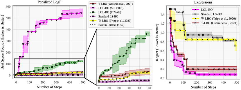
In Figure 1, we plot the cumulative best objective value for the penalized log P and expressions tasks, averaged over three runs. For log P, LOL-BO using the SELFIES transformer VAE achieves an average log P score of 545.17 after 500 iterations. Using a JTVAE, which is more directly comparable to prior work, we still achieve an average score of 123.54–higher than previous state-of-the-art scores using latent space BO of 26.11 [14]. For the expressions task, LOL-BO achieves a final regret of 0.079 on average, versus 0.194 achieved by T-LBO.
Molecule quality.
While molecules found using LOL-BO for the log P task are “valid” according to software commonly used to compute these scores, the molecules produced by this search clearly abandon any notion of reality. A number of methods have been proposed to evaluate molecule quality [3], and indeed even some recent work in LS-BO has explored encouraging higher quality solutions [35]. However, our primary goal in this paper is to develop stronger optimization routines in this space, and indeed the baselines we consider also treat log P as an unconstrained optimization problem. Therefore, this result should be taken primarily as evidence that the log P objective can be exploited by a sufficiently strong optimizer, rather than as evidence of novel interesting molecules.
5.2 Guacamol Benchmark Tasks
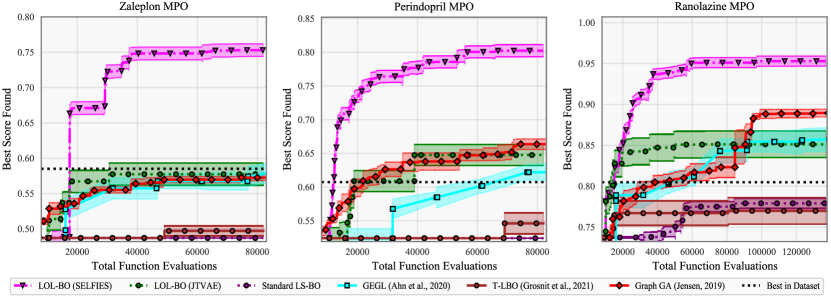
The Guacamol222Guacamol is released under the MIT license benchmark suite [3] contains scoring oracles for a variety of molecule design tasks, with scores ranging between 0 and 1. We select three tasks among the most challenging in terms of the best objective value achieved: Perindopril MPO, Ranolazine MPO, and Zaleplon MPO. The goal of each of these tasks is to design a molecule with high fingerprint similarity to a known target drug but that differs in a specified target way. The task definitions are discussed in Brown et al. [3].
Baselines.
We compare to T-LBO, the most competitive Bayesian optimization method overall from subsection 5.1. Additionally, a variety of techniques from beyond the BO literature using reinforcement learning and genetic programming have been evaluated on these tasks. We compare to GEGL and GraphGA, with GraphGA [20] among the top methods on the Guacamol leaderboard. We also report the best score achieved over the 1.27 million molecules in the full Guacamol dataset, which serves as a performance cap for virtual screening (see section 4).
Results.
The results of optimization on these three benchmarks are shown in Figure 2. We again report results for LOL-BO with both a JTVAE and SELFIES VAE deep autoencoder. LOL-BO with a SELFIES VAE optimizes significantly faster than other methods in the evaluation budget used here.
5.3 DRD3 Receptor Docking Affinity
| SELFIES VAE | JTVAE | |
|---|---|---|
| Reconstruction Acc. | 0.913 | 0.767 |
| Avg. Decode Time (s) | 0.02 | 3.14 |
| Decode Stddev | 0.04 | 0.1 |
| Validity | 1.0 | 1.0 |
| GP Test NLL (Perindopril) | -2.156 | -1.481 |
| GP Test NLL(Zaleplon) | -2.705 | -1.781 |
| GP Test NLL (Ranolazine) | -2.127 | -1.649 |
| Method | Best Score Found in Evaluation Budget | |||
|---|---|---|---|---|
| 100 evals | 500 evals | 1000 evals | 5000 evals | |
| LOL-BO (SELFIES) | ||||
| TuRBO (SELFIES) | ||||
| LS-BO (SELFIES) | ||||
| LOL-BO (JTVAE) | ||||
| TuRBO (JTVAE) | ||||
| LS-BO (JTVAE) | ||||
| T-LBO | ||||
| Graph-GA | ||||
| SMI-LSTM | ||||
| MARS | ||||
| MolDQN | ||||
| GCPN | ||||
The Therapeutics Data Commons (TDC) benchmark suite [17] contains oracles that evaluate the binding propensity of a ligand (small molecule) to a target protein. These docking oracles incur nontrivial computation cost, requiring on the order of minutes to evaluate, making them ideal benchmark tasks for Bayesian optimization. In this paper, we focus on designing ligands that bind to dopamine receptor D3 (DRD3), as the TDC website maintains a leaderboard of results for DRD3 333https://tdcommons.ai/benchmark/docking_group/drd3/. We compare LOL-BO on the DRD3 docking task to the TDC leaderboard and three BO methods–T-LBO, standard LS-BO, and fixed latent space TuRBO on this task.
Results of optimization are in Table Table 1 (right). LOL-BO achieves the best performance among the BO baselines, with only TuRBO making significant progress on the task by 5000 evaluations. Compared to the baselines from the TDC leaderboard, LOL-BO is significantly more sample efficient, achieving results comparable to the best method with a factor of fewer oracle calls.
5.4 Ablation studies
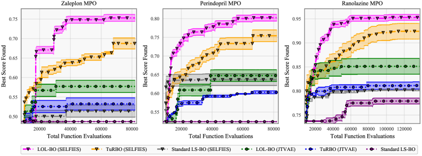
In this section, we evaluate the components of LOL-BO described in subsection 3.2 beyond the direct application of TuRBO in the latent space described in subsection 3.1. We run TuRBO on the three Guacamol tasks considered in subsection 5.2 using a fixed latent space extracted by the pretrained SELFIES VAE and JTVAE. To run TuRBO, we use the same experimental setup as for LOL-BO, but and are fixed at the start of optimization. We compare LS-BO, TuRBO, and LOL-BO on all three tasks in Figure 3. The use of SVGP is controlled across methods.
LOL-BO outperforms TuRBO across all DAE models and tasks. While these results demonstrate the impact of joint training, the excellent performance of TuRBO in a static, pre-trained latent space highlights the value of high dimensional Bayesopt in this setting.
To further analyze whether the jointly trained latent space better-matches the distance based assumptions of the GP model, we include an additional analysis directly comparing scores of molecules sampled from a local region around the top-scoring molecule in the latent space of the pretrained SELFIES-VAE before optimization has begun and at the end of optimization (see subsection A.3).
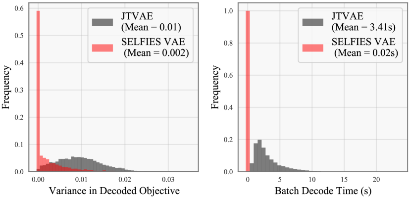
Since LOL-BO achieves better performance with the SELFIES VAE than with the JTVAE, we evaluate a series of metrics for both DAE models. In Table Table 1 left, we compare reconstruction error and validity, as well as the standard deviation in Perindopril MPO score from decoding a fixed latent vector 20 times, averaged over 3500 distinct . We report supervised learning performance for a GP trained on molecules taken from the initial Guacamol dataset, using the pretrained latent spaces. Across standard metrics, the SELFIES VAE achieves excellent performance. Beyond these, the improvement in objective variance for a single is notable: because Guacamol objective values are in the range , a standard deviation of represents significant additional noise. Thus, the DAE can be a significant source of noise even for an otherwise deterministic objective function.
6 Conclusion
Designing latent spaces for Bayesian optimization is challenging because the VAE and the optimizer often compete: too small of a latent space renders the VAE incapable of capturing the structure present in the input space, while too large a latent space makes optimization challenging.
The empirical results we present here demonstrate the importance of viewing these latent spaces as high-dimensional and tackling optimization with high-dimensional BO strategies, even though these latent spaces are often significantly smaller than the input space. Furthermore, we show that high-dimensional BO methods can be significantly improved when translating them to the latent space setting, demonstrating the potential of further research at the intersection of these areas.
7 Acknowledgements
JRG and NM were supported by NSF award IIS-2145644. JM and HJ were supported by the Laboratory Directed Research and Development program of Los Alamos National Laboratory (LANL) under project number 20210043DR.
References
- Ahn et al. [2020] Sungsoo Ahn, Junsu Kim, Hankook Lee, and Jinwoo Shin. Guiding deep molecular optimization with genetic exploration, 2020.
- Balandat et al. [2020] Maximilian Balandat, Brian Karrer, Daniel R. Jiang, Samuel Daulton, Benjamin Letham, Andrew Gordon Wilson, and Eytan Bakshy. BoTorch: A Framework for Efficient Monte-Carlo Bayesian Optimization. In Advances in Neural Information Processing Systems 33, 2020. URL http://arxiv.org/abs/1910.06403.
- Brown et al. [2019] Nathan Brown, Marco Fiscato, Marwin H.S. Segler, and Alain C. Vaucher. Guacamol: Benchmarking models for de novo molecular design. Journal of Chemical Information and Modeling, 59(3):1096–1108, Mar 2019. ISSN 1549-960X. doi: 10.1021/acs.jcim.8b00839. URL http://dx.doi.org/10.1021/acs.jcim.8b00839.
- Dai et al. [2018] Hanjun Dai, Yingtao Tian, Bo Dai, Steven Skiena, and Le Song. Syntax-Directed variational autoencoder for structured data. In International Conference on Learning Representations 2018, 2018.
- Deshwal and Doppa [2021] Aryan Deshwal and Janardhan Rao Doppa. Combining latent space and structured kernels for Bayesian optimization over combinatorial spaces. CoRR, abs/2111.01186, 2021. URL https://arxiv.org/abs/2111.01186.
- Eissman et al. [2018] Stephan Eissman, Daniel Levy, Rui Shu, Stefan Bartzsch, and Stefano Ermon. Bayesian optimization and attribute adjustment. In Proc. 34th Conference on Uncertainty in Artificial Intelligence, 2018.
- Eriksson and Jankowiak [2021] David Eriksson and Martin Jankowiak. High-dimensional Bayesian optimization with sparse axis-aligned subspaces. arXiv preprint arXiv:2103.00349, 2021.
- Eriksson et al. [2019] David Eriksson, Michael Pearce, Jacob Gardner, Ryan D Turner, and Matthias Poloczek. Scalable global optimization via local Bayesian optimization. In H. Wallach, H. Larochelle, A. Beygelzimer, F. d'Alché-Buc, E. Fox, and R. Garnett, editors, Advances in Neural Information Processing Systems, volume 32. Curran Associates, Inc., 2019. URL https://proceedings.neurips.cc/paper/2019/file/6c990b7aca7bc7058f5e98ea909e924b-Paper.pdf.
- Gardner et al. [2017] Jacob Gardner, Chuan Guo, Kilian Weinberger, Roman Garnett, and Roger Grosse. Discovering and exploiting additive structure for Bayesian optimization. In Artificial Intelligence and Statistics, pages 1311–1319. PMLR, 2017.
- Gardner et al. [2018] Jacob R Gardner, Geoff Pleiss, David Bindel, Kilian Q Weinberger, and Andrew Gordon Wilson. Gpytorch: Blackbox matrix-matrix Gaussian process inference with GPU acceleration. arXiv preprint arXiv:1809.11165, 2018.
- Garnett et al. [2014] Roman Garnett, Michael A Osborne, and Philipp Hennig. Active learning of linear embeddings for Gaussian processes. Proceedings of the Thirtieth Conference on Uncertainty in Artificial Intelligence, 2014.
- Gómez-Bombarelli et al. [2018] Rafael Gómez-Bombarelli, Jennifer N Wei, David Duvenaud, José Miguel Hernández-Lobato, Benjamín Sánchez-Lengeling, Dennis Sheberla, Jorge Aguilera-Iparraguirre, Timothy D Hirzel, Ryan P Adams, and Alán Aspuru-Guzik. Automatic chemical design using a data-driven continuous representation of molecules. ACS central science, 4(2):268–276, 2018.
- Graff et al. [2021] David E Graff, Eugene I Shakhnovich, and Connor W Coley. Accelerating high-throughput virtual screening through molecular pool-based active learning. Chemical science, 12(22):7866–7881, April 2021.
- Grosnit et al. [2021] Antoine Grosnit, Rasul Tutunov, Alexandre Max Maraval, Ryan-Rhys Griffiths, Alexander Imani Cowen-Rivers, Lin Yang, Lin Zhu, Wenlong Lyu, Zhitang Chen, Jun Wang, Jan Peters, and Haitham Bou-Ammar. High-dimensional Bayesian optimisation with variational autoencoders and deep metric learning. CoRR, abs/2106.03609, 2021. URL https://arxiv.org/abs/2106.03609.
- Hensman et al. [2013] James Hensman, Nicolo Fusi, and Neil D Lawrence. Gaussian processes for big data. Proceedings of the Twenty-Ninth Conference on Uncertainty in Artificial Intelligence, 2013.
- Hernández-Lobato et al. [2017] José Miguel Hernández-Lobato, James Requeima, Edward O Pyzer-Knapp, and Alán Aspuru-Guzik. Parallel and distributed Thompson sampling for large-scale accelerated exploration of chemical space. In Doina Precup and Yee Whye Teh, editors, Proceedings of the 34th International Conference on Machine Learning, volume 70, pages 1470–1479. PMLR, 2017.
- Huang et al. [2021] Kexin Huang, Tianfan Fu, Wenhao Gao, Yue Zhao, Yusuf Roohani, Jure Leskovec, Connor W Coley, Cao Xiao, Jimeng Sun, and Marinka Zitnik. Therapeutics data commons: Machine learning datasets and tasks for drug discovery and development. Proceedings of Neural Information Processing Systems, NeurIPS Datasets and Benchmarks, 2021.
- Irwin and Shoichet [2005] John J Irwin and Brian K Shoichet. Zinc- a free database of commercially available compounds for virtual screening. Journal of chemical information and modeling, 45(1):177–182, 2005.
- Irwin et al. [2020] John J Irwin, Khanh G Tang, Jennifer Young, Chinzorig Dandarchuluun, Benjamin R Wong, Munkhzul Khurelbaatar, Yurii S Moroz, John Mayfield, and Roger A Sayle. Zinc20—a free ultralarge-scale chemical database for ligand discovery. Journal of chemical information and modeling, 60(12):6065–6073, 2020.
- Jensen [2019] JH Jensen. A graph-based genetic algorithm and generative model/Monte Carlo tree search for the exploration of chemical space. chem sci 10 (12): 3567–3572, 2019.
- Jin et al. [2018] Wengong Jin, Regina Barzilay, and Tommi S. Jaakkola. Junction tree variational autoencoder for molecular graph generation. In International Conference on Machine Learning. PMLR, 2018.
- Kajino [2019] Hiroshi Kajino. Molecular hypergraph grammar with its application to molecular optimization. In International Conference on Machine Learning, pages 3183–3191. PMLR, 2019.
- Kandasamy et al. [2015] Kirthevasan Kandasamy, Jeff Schneider, and Barnabás Póczos. High dimensional Bayesian optimisation and bandits via additive models. In International conference on machine learning, pages 295–304. PMLR, 2015.
- Kingma and Welling [2013] Diederik P Kingma and Max Welling. Auto-encoding variational Bayes. arXiv preprint arXiv:1312.6114, 2013.
- Kingma et al. [2014] Diederik P Kingma, Shakir Mohamed, Danilo Jimenez Rezende, and Max Welling. Semi-supervised learning with deep generative models. In Advances in neural information processing systems, pages 3581–3589, 2014.
- Kirkpatrick and Ellis [2004] Peter Kirkpatrick and Clare Ellis. Chemical space. Nature, 432(7019):823–823, December 2004.
- Krenn et al. [2019] Mario Krenn, Florian Häse, AkshatKumar Nigam, Pascal Friederich, and Alán Aspuru-Guzik. SELFIES: a robust representation of semantically constrained graphs with an example application in chemistry. CoRR, abs/1905.13741, 2019. URL http://arxiv.org/abs/1905.13741.
- Kusner et al. [2017] Matt J Kusner, Brooks Paige, and José Miguel Hernández-Lobato. Grammar variational autoencoder. In International Conference on Machine Learning, pages 1945–1954. PMLR, 2017.
- Lu et al. [2018] Xiaoyu Lu, Javier Gonzalez, Zhenwen Dai, and Neil Lawrence. Structured variationally auto-encoded optimization. In Jennifer Dy and Andreas Krause, editors, Proceedings of the 35th International Conference on Machine Learning, volume 80 of Proceedings of Machine Learning Research, pages 3267–3275, Stockholmsmässan, Stockholm Sweden, 2018. PMLR.
- Mockus [1982] Jonas Mockus. The Bayesian approach to global optimization. In System Modeling and Optimization, pages 473–481. Springer, 1982.
- Mouchlis et al. [2021] Varnavas D Mouchlis, Antreas Afantitis, Angela Serra, Michele Fratello, Anastasios G Papadiamantis, Vassilis Aidinis, Iseult Lynch, Dario Greco, and Georgia Melagraki. Advances in de novo drug design: from conventional to machine learning methods. International journal of molecular sciences, 22(4):1676, 2021.
- Nayebi et al. [2019] Amin Nayebi, Alexander Munteanu, and Matthias Poloczek. A framework for Bayesian optimization in embedded subspaces. In International Conference on Machine Learning, pages 4752–4761. PMLR, 2019.
- Nelder and Mead [1965] John A Nelder and Roger Mead. A simplex method for function minimization. The computer journal, 7(4):308–313, 1965.
- Nigam et al. [2020] Akshatkumar Nigam, Pascal Friederich, Mario Krenn, and Alan Aspuru-Guzik. Augmenting genetic algorithms with deep neural networks for exploring the chemical space. In International Conference on Learning Representations, 2020.
- Notin et al. [2021] Pascal Notin, José Miguel Hernández-Lobato, and Yarin Gal. Improving black-box optimization in VAE latent space using decoder uncertainty. Advances in Neural Information Processing Systems, 34, 2021.
- Olivecrona et al. [2017] Marcus Olivecrona, Thomas Blaschke, Ola Engkvist, and Hongming Chen. Molecular de-novo design through deep reinforcement learning. Journal of cheminformatics, 9(1):48, September 2017.
- Osborne et al. [2009] Michael A Osborne, Roman Garnett, and Stephen J Roberts. Gaussian processes for global optimization. In 3rd international conference on learning and intelligent optimization (LION3), pages 1–15, 2009.
- Samanta et al. [2019] Bidisha Samanta, Abir De, Gourhari Jana, Pratim Kumar Chattaraj, Niloy Ganguly, and Manuel Gomez-Rodriguez. NeVAE: A deep generative model for molecular graphs. In Proceedings of the AAAI Conference on Artificial Intelligence, volume 33 of 01, pages 1110–1117, 2019.
- Segler et al. [2018] Marwin H. S. Segler, Thierry Kogej, Christian Tyrchan, and Mark P. Waller. Generating focused molecule libraries for drug discovery with recurrent neural networks. ACS Central Science, 4(1):120–131, 2018. doi: 10.1021/acscentsci.7b00512. URL https://doi.org/10.1021/acscentsci.7b00512. PMID: 29392184.
- Siivola et al. [2021] Eero Siivola, Andrei Paleyes, Javier González, and Aki Vehtari. Good practices for Bayesian optimization of high dimensional structured spaces. Applied AI Letters, 2(2):e24, 2021.
- Snoek et al. [2012] Jasper Snoek, Hugo Larochelle, and Ryan P Adams. Practical Bayesian optimization of machine learning algorithms. Advances in neural information processing systems, 25, 2012.
- Titsias [2009] Michalis Titsias. Variational learning of inducing variables in sparse Gaussian processes. In Artificial intelligence and statistics, pages 567–574. PMLR, 2009.
- Tripp et al. [2020] Austin Tripp, Erik A. Daxberger, and José Miguel Hernández-Lobato. Sample-efficient optimization in the latent space of deep generative models via weighted retraining. In Advances in Neural Information Processing Systems 33, 2020.
- Urbina et al. [2020] Fabio Urbina, Filippa Lentzos, Cédric Invernizzi, and Sean Ekins. Dual use of artificial-intelligence-powered drug discovery. Nature machine intelligence, 4:189–191, 2020.
- van Hilten et al. [2019] Niek van Hilten, Florent Chevillard, and Peter Kolb. Virtual compound libraries in Computer-Assisted drug discovery. Journal of chemical information and modeling, 59(2):644–651, February 2019.
- Vaswani et al. [2017] Ashish Vaswani, Noam Shazeer, Niki Parmar, Jakob Uszkoreit, Llion Jones, Aidan N Gomez, Łukasz Kaiser, and Illia Polosukhin. Attention is all you need. In Advances in neural information processing systems, pages 5998–6008, 2017.
- Wang et al. [2018] Zi Wang, Clement Gehring, Pushmeet Kohli, and Stefanie Jegelka. Batched large-scale Bayesian optimization in high-dimensional spaces. In International Conference on Artificial Intelligence and Statistics, pages 745–754. PMLR, 2018.
- Wang et al. [2016] Ziyu Wang, Frank Hutter, Masrour Zoghi, David Matheson, and Nando de Feitas. Bayesian optimization in a billion dimensions via random embeddings. Journal of Artificial Intelligence Research, 55:361–387, 2016.
- Weininger [1988] David Weininger. SMILES, a chemical language and information system. 1. introduction to methodology and encoding rules. Journal of Chemical Information and Computer Sciences, 28(1):31–36, 1988. doi: 10.1021/ci00057a005. URL https://pubs.acs.org/doi/abs/10.1021/ci00057a005.
- Williams et al. [2015] Kevin Williams, Elizabeth Bilsland, Andrew Sparkes, Wayne Aubrey, Michael Young, Larisa N Soldatova, Kurt De Grave, Jan Ramon, Michaela de Clare, Worachart Sirawaraporn, Stephen G Oliver, and Ross D King. Cheaper faster drug development validated by the repositioning of drugs against neglected tropical diseases. Journal of the Royal Society, Interface / the Royal Society, 12(104):20141289, March 2015.
- Wilson et al. [2016a] Andrew G Wilson, Zhiting Hu, Russ R Salakhutdinov, and Eric P Xing. Stochastic variational deep kernel learning. Advances in Neural Information Processing Systems, 29:2586–2594, 2016a.
- Wilson et al. [2016b] Andrew Gordon Wilson, Zhiting Hu, Ruslan Salakhutdinov, and Eric P Xing. Deep kernel learning. In Artificial intelligence and statistics, pages 370–378. PMLR, 2016b.
- Xie et al. [2021] Yutong Xie, Chence Shi, Hao Zhou, Yuwei Yang, Weinan Zhang, Yong Yu, and Lei Li. MARS: Markov molecular sampling for multi-objective drug discovery. In International Conference on Learning Representations, 2021.
- You et al. [2018] Jiaxuan You, Bowen Liu, Zhitao Ying, Vijay Pande, and Jure Leskovec. Graph convolutional policy network for Goal-Directed molecular graph generation. In S Bengio, H Wallach, H Larochelle, K Grauman, N Cesa-Bianchi, and R Garnett, editors, Advances in Neural Information Processing Systems 31, pages 6410–6421. Curran Associates, Inc., 2018.
- Zhang et al. [2019] Muhan Zhang, Shali Jiang, Zhicheng Cui, Roman Garnett, and Yixin Chen. D-VAE: A variational autoencoder for directed acyclic graphs. In Advances in Neural Information Processing Systems 32, pages 1588–1600. Curran Associates, Inc., 2019.
- Zhou et al. [2019] Zhenpeng Zhou, Steven Kearnes, Li Li, Richard N Zare, and Patrick Riley. Optimization of molecules via deep reinforcement learning. Scientific reports, 9(1):10752, July 2019.
Checklist
-
1.
For all authors…
-
(a)
Do the main claims made in the abstract and introduction accurately reflect the paper’s contributions and scope? [Yes]
-
(b)
Did you describe the limitations of your work? [Yes] (see subsection A.7)
-
(c)
Did you discuss any potential negative societal impacts of your work? [Yes] (see subsection A.7)
-
(d)
Have you read the ethics review guidelines and ensured that your paper conforms to them? [Yes]
-
(a)
-
2.
If you are including theoretical results…
-
(a)
Did you state the full set of assumptions of all theoretical results? [N/A]
-
(b)
Did you include complete proofs of all theoretical results? [N/A]
-
(a)
-
3.
If you ran experiments…
-
(a)
Did you include the code, data, and instructions needed to reproduce the main experimental results (either in the supplemental material or as a URL)? [Yes] (See section 5 where we will provide a link to a github repository with our code)
-
(b)
Did you specify all the training details (e.g., data splits, hyperparameters, how they were chosen)? [Yes] (See section 5)
-
(c)
Did you report error bars (e.g., with respect to the random seed after running experiments multiple times)? [Yes] (See section 5)
-
(d)
Did you include the total amount of compute and the type of resources used (e.g., type of GPUs, internal cluster, or cloud provider)? [Yes] (See subsection A.4)
-
(a)
-
4.
If you are using existing assets (e.g., code, data, models) or curating/releasing new assets…
-
(a)
If your work uses existing assets, did you cite the creators? [Yes] (See section 5)
-
(b)
Did you mention the license of the assets? [Yes] (See subsection A.5)
-
(c)
Did you include any new assets either in the supplemental material or as a URL? [Yes] (See section 5 where we will provide a link to a github repository with our code)
-
(d)
Did you discuss whether and how consent was obtained from people whose data you’re using/curating? [N/A]
-
(e)
Did you discuss whether the data you are using/curating contains personally identifiable information or offensive content? [N/A]
-
(a)
-
5.
If you used crowdsourcing or conducted research with human subjects…
-
(a)
Did you include the full text of instructions given to participants and screenshots, if applicable? [N/A]
-
(b)
Did you describe any potential participant risks, with links to Institutional Review Board (IRB) approvals, if applicable? [N/A]
-
(c)
Did you include the estimated hourly wage paid to participants and the total amount spent on participant compensation? [N/A]
-
(a)
Appendix A Appendix
A.1 Additional implementation details
As the data collected by LOL-BO grows, it becomes increasingly computationally expensive to update the models in and end-to-end fashion on all of the data. Thus, instead of updating on all data, we only update end-to-end on a subset of the data consisting of the most recently collected batch of data points, plus the top- scoring points from the remaining data. For the experiments in subsection 5.1 and subsection 5.3 where we have a small evaluation budget, we use . For the experiments in subsection 5.2 with a larger total evaluation budget, we use .
A.2 JTVAE vs. SELFIES VAE additional analysis
In Figure 4, we provide histograms to visualize a few of the statistics summarized in Table 1 in the main text Table 1.
A.3 Additional ablation analysis
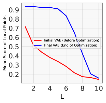
In this section, we analyze whether the jointly trained latent space matches the distance based assumptions of the GP model. On the Ranolazine MPO task, we first encode the best molecule (score=0.9382) from a single run of LOL-BO to get the latent codes and from both the pretrained VAE before optimization has begun and at the end of optimization. We then analyze the average score of molecules decoded from latent vectors sampled uniformly from an -hypercube centered at both and . By , latent codes in the joint VAE near still achieve an average score of 0.9106, while for vectors near in the pretrained model the average score has dropped to only 0.3382 Figure 5.
In this section, we additionally analyze whether the jointly trained VAE is better able to reconstruct the highest-scoring molecules found by the optimizer. Empirically, the optimizer consistently produces higher-scoring molecules than any found in the entire initial unsupervised dataset used to train the initial VAE (see Best in Dataset comparison in Figure 2). This raises the question of whether these high-scoring molecules found by the optimizer may often be out-of-sample for the initial VAE. To investigate this, we took the top highest-scoring molecules found by LOL-BO on the Ranolazine MPO task and computed the reconstruction accuracy of the initial VAE on these molecules. We repeated this experiment with the final VAE obtained at the end of the optimization run. We found that the average reconstruction accuracy of the initial VAE was while the average accuracy of the final VAE was . The extremely low reconstruction accuracy of the initial VAE indicates that many of the high-scoring molecules found by the optimizer are indeed out-of-sample. It would therefore be very difficult to find these high-scoring molecules by simply searching in the latent space of the initial VAE. In contrast, finding these high-scoring molecules by searching in the latent space of the final VAE would likely be much easier. Therefore, this result provides further motivation for our procedure of jointly updating the VAE during optimization, so that as the optimization proceeds, the VAE is made to adapt so that it can better construct the types of moleucles we are interested in, even if they are unlike any molecules in the initial unsupervised dataset.
A.4 Compute
The SELFIES VAE was trained using a single server with eight Quadro RTX 8000 GPUs. All optimization experiments were run on a single RTX A5000 GPU. We used an internal cluster for compute.
A.5 Software licensing
All major software packages used (ie BoTorch, GPyTorch, Guacamol) are released under MIT license.
A.6 Run-time considerations
LOL-BO scales to large evaluation settings readily via minibatch training of the ELBO in Equation 4 due to the variational GP approximation used (Hensman et al., 2013). TuRBO scales similarly by using the same variational GP approximation. Although we’ve shown that LOL-BO significantly improves performance over TuRBO (see Figure 5), it is important to consider the additional time complexity of LOL-BO. In particular, updating the VAE jointly can add significant time complexity, particularly with very deep transformers. However, this cost is generally manageable since relatively little VAE updating is required with the small amount of data acquired at each step (compared to the initial training on the large unsupervised dataset).
When the evaluation budget is small (Section 5.1), or the objective function expensive (Section 5.3), LOL-BO incurs as little as a 1.01 slowdown over running TuRBO. However, larger evaluation budgets require retraining the encoder on growing amounts of data. Thus, in Section 5.2, we do incur as much as a slowdown in the worst case. However, the total running time in Section 5.2 is still typically on the order of half a day, and we believe the improved outer-loop optimization performance makes the additional time complexity worthwhile. Finally, the added cost of jointly updating the VAE is negligible compared to the cost of certain oracle calls typical in molecule design. For instance, in Section 5.3 the docking oracle takes minutes to evaluate per molecule, leading to run-times of up to a few days, and even this would be considered cheap compared to wet-lab experiments. To see specific wall-clock times for all methods, see Table 2. The wall clock times given for W-LBO [43] were obtained with our modifications to parallelize the W-LBO code-base.
| Method | Avg. Wall Clock Runtime (hours) | |||
| Penalized Log P (Sec. 5.1) | Expressions (Sec. 5.1) | GuacaMol (Sec. 5.2) | Docking (Sec. 5.3) | |
| LOL-BO (SELFIES) | NA | |||
| TuRBO (SELFIES) | NA | |||
| LS-BO (SELFIES) | NA | |||
| LOL-BO (JTVAE) | NA | |||
| TuRBO (JTVAE) | NA | |||
| LS-BO (JTVAE) | NA | |||
| LOL-BO (Grammar VAE) | NA | NA | NA | |
| TuRBO (Grammar VAE) | NA | NA | NA | |
| LS-BO (Grammar VAE) | NA | NA | NA | |
| T-LBO | ||||
| W-LBO | NA | NA | ||
| GEGL | NA | NA | NA | |
| Graph-GA | NA | NA | NA | |
A.7 Potential limitations and future work
This work focuses on molecular optimization tasks centered around drug development. While the development of new drugs has the potential to help many people, it is also important to consider the dual use nature of such methods. In particular, AI technologies for drug discovery have the potential to be misused for the de novo design of biochemical weapons [44]. It is also important to consider the potential for negative societal impact if any new drugs discovered are not property tested before being administered. While we hope that our work can eventually speed-up the drug development process by providing useful candidate molecules, it is essential that experts remain heavily involved and that FDA guidelines for drug development and approval are strictly adhered to.
Additionally, the oracles and tasks we use here, even ones with the potential to design candidate drug molecules like protein docking, are completely oblivious to critical aspects like human safety and efficacy, stability, manufacturing cost, and so on. These computational approaches to molecule design should therefore be considered first pass screening procedures, not procedures to design final end products.
In order to optimize the Guacamol molecular optimization tasks, LOL-BO requires tens of thousands of function evaluations Figure 2. While the fairly cheap Guacamol oracles have made it reasonable to do this many evaluations, there are many molecule design applications where each function evaluation is much more expensive. In particular, tens of thousands of function evaluations is likely not efficient enough for many applications that would be run in vitro with actual wet-lab experiments.
Another potential limitation of LOL-BO is that is is designed to find a single best optima for a given task. However, in the molecular space in particular, it is often desirable to find multiple good optima since a single solution might fail for unknown reasons downstream. In future work, we plan to explore methods that can be used to extend Bayesian optimization to obtain a set of diverse solutions rather than a single solution.