Multiple-Source Domain Adaptation via Coordinated Domain Encoders and Paired Classifiers

Abstract

We present a novel multiple-source unsupervised model for text classification under domain shift. Our model exploits the update rates in document representations to dynamically integrate domain encoders. It also employs a probabilistic heuristic to infer the error rate in the target domain in order to pair source classifiers. Our heuristic exploits data transformation cost and the classifier accuracy in the target feature space. We have used real world scenarios of Domain Adaptation to evaluate the efficacy of our algorithm. We also used pretrained multi-layer transformers as the document encoder in the experiments to demonstrate whether the improvement achieved by domain adaptation models can be delivered by out-of-the-box language model pretraining. The experiments testify that our model is the top performing approach in this setting.

1 Introduction

Modern classifiers typically rely on large amount of training data. Collecting large training sets is expensive and in some cases very challenging, e.g., in legal domain (Holzenberger, Blair-Stanek, and Van Durme 2020) or in social media domain (Karisani, Choi, and Xiong 2021; Karisani and Karisani 2020). There exist several techniques to address the lack of training data, one of which is Domain Adaptation (Ben-David and Schuller 2003), where a classifier is trained in one domain (the source domain) and evaluated in another domain (the target domain). One of the fundamental assumptions of text classification is that training and test data follow an identical distribution. A classifier trained in one domain, typically is a poor predictor for another domain (Ben-David et al. 2010). Therefore, Domain Adaptation primarily tackles the domain shift challenge (Torralba and Efros 2011). One of the major areas of Domain Adaptation, which is also the subject of our study, is the unsupervised setting where there is no labeled target data available.

Theoretical studies (Ben-David et al. 2010) have shown that the outcome of Domain Adaptation is primarily influenced by the performance of the classifier in the source domain and the discrepancy between the source and the target domains. The former can be improved irrespective of domain shift, therefore, existing domain adaptation models primarily focus on the latter. These models approach the task either explicitly by minimizing the divergence between the two distributions (Long et al. 2015) or via a binary classifier to increase the domain confusion and to reduce the divergence (Ganin and Lempitsky 2015). In either case, the aim is to obtain domain-invariant features between the source and the target (Yosinski et al. 2014).

In this article, we study multiple-source Domain Adaptation (Mansour, Mohri, and Rostamizadeh 2009). In this setting, there are multiple labeled source domains available and the goal is to minimize the classification error in the target domain. While the availability of multiple sources provides us with more opportunities, this also comes with challenges. Naively applying single-source domain adaptation models in a multiple-source setting may cause negative transfer (Pan and Yang 2010), i.e., deterioration in performance. In this work, we propose an objective function to minimize negative transfer via the coordination between the representations of source domains. Additionally, based on the intuition that every source classifier may specialize in predicting some regions of the target domain, we present a heuristic criterion to guide the weak source classifiers by the reliable ones.

We evaluate our model in two datasets consisting of user-generated data in Twitter. We select this domain because it is considerably less explored compared to other domains, e.g., sentiment analysis. The documents in this domain are short and their language is highly informal (Karisani, Agichtein, and Ho 2020). Additionally, due to the nature of the tasks in this domain the class distributions are typically imbalanced (Karisani and Agichtein 2018). Taken together, these are significant challenges for existing methods. The results in this setting testify that our model is the most robust approach across various cases and consistently outperforms multiple state of the art baselines.

2 Related Work

Mansour, Mohri, and Rostamizadeh (2009) theoretically show that, in multiple-source domain adaptation setting, simply combining the source classifiers yields a high prediction error. They show that there always exists a weighted average of the source classifiers that has a low error prediction in the target domain–their weights are derived from the source distributions. Therefore, existing multiple-source models typically rely on either inventively aggregating source data (Guo, Shah, and Barzilay 2018) or crafting source classifiers (Xu et al. 2018). While studies occasionally make an attempt to theoretically justify their approach (Long et al. 2015), majority of existing domain adaptation studies rely on intuitions and heuristics (Tzeng et al. 2017; Zhao et al. 2020; Isobe et al. 2021). In this work, we show the same pragmatism and propose an intuitive objective function to reduce the risk of negative transfer, and also present a probabilistic heuristic to encourage the collaboration between source classifiers.

Our model, which we call Coordinated Encoders and Paired Classifiers (CEPC ​), possesses two distinct qualities. First, it employs the intuitive idea of coordination between source encoders. The aim of coordination is to organize source domains such that the domains with similar characteristics share the same encoder. Existing studies resort to different approaches. For instance, Peng et al. (2019) share one encoder between all source domains, however, aim to reduce the discrepancy between them via a new loss term. Guo, Pasunuru, and Bansal (2020) incorporate multiple discrepancy terms and dynamically select source domains. Yang et al. (2020a) dynamically select data points and Wright and Augenstein (2020) dynamically aggregate source classifiers.

The second quality of our model is to exploit the properties of source data to pair source classifiers via a heuristic criterion. Here, we aim to guide the weak classifiers by the more reliable ones, therefore, the weak classifiers can adjust their class boundaries based on the information that is not available in their training data. Previous studies have explored the interaction between source classifiers using different approaches. Zhao et al. (2020) adversarially train source classifiers and use the distance between source and target domains to fine-tune their model. Different from their work, in our model source classifiers are paired and can interact. Isobe et al. (2021) employ the KL divergence term as an objective term, however, their model is developed for the multi-target setting. Other relevant approaches in this area include combining semi-supervised learning and unsupervised domain adaptation to guide source classifiers (Yang et al. 2020b), and using attention mechanism to assign target data points to source domains (Cui and Bollegala 2020).

3 Proposed Method

In multiple-source unsupervised domain adaptation, we are given a set of $M$ source domains $S_{1},S_{2},\dotsc,S_{M}$ denoted by ${\{(\textsc{x}_{i}^{s_{j}},y_{i}^{s_{j}})\}}_{i=1}^{n_{s_{j}}}$ where $(\textsc{x}_{i}^{s_{\mathord{\color[rgb]{0.67,0.67,0.67}\bullet}}},y_{i}^{s_{\mathord{\color[rgb]{0.67,0.67,0.67}\bullet}}})$ is the i-th labeled document in $S_{\mathord{\color[rgb]{0.67,0.67,0.67}\bullet}}$ and $n_{s_{\mathord{\color[rgb]{0.67,0.67,0.67}\bullet}}}$ is the number of documents in $S_{\mathord{\color[rgb]{0.67,0.67,0.67}\bullet}}$. We are also given a target domain $T$ denoted by ${\{\textsc{x}_{i}^{t}\}}_{i=1}^{n_{t}}$, where $\textsc{x}_{i}^{t}$ is the i-th unlabeled document and $n_{t}$ is the number of documents in the domain $T$. The aim is to train a model which minimizes the prediction error in the target domain using the labeled source data. Note that the distributions of the documents in the source domains and the target domain are different, thus, a classifier trained on the source domains is typically a poor predictor for the target domain.

Figure 1 illustrates our model (CEPC ​). Here, we assume that there are three source domains available. For each source domain, there is an encoder ($E$) and a classifier ($C$). Each pair is trained by three objective terms, namely: the classification loss, the discrepancy loss, and the divergence loss. The classification loss, which is the Negative Log-Likelihood, quantifies the calibration error of the classifier in the labeled source data. The discrepancy loss, quantifies the variation between the distribution of the encoded source and target documents, and the divergence loss, which quantifies the inconsistency between the output of source classifiers. The dashed lines indicate shared parameters between the modules. At test time, the source classifiers–along their corresponding encoders–are used to label target documents, and a majority voting is used to obtain the final labels.

Figure 1: Overview of our model for a task with three source domains. The output of each domain encoder is used in the corresponding source classifier. To train each pair of (encoder, classifier) three loss terms are minimized: 1) the regular classification loss, 2) the discrepancy loss between the encoded source and target data (see Section 3.5), and 3) the divergence loss between the output of the source classifiers (see Section 3.2). The dashed line indicate shared parameters (see Section 3.1).

The encoder in our model is employed to project documents into a shared low-dimensional space. For the discussion about the classification and the discrepancy loss terms see Section 3.5. Here, we discuss the divergence loss, which aims to minimize the inconsistency between source classifiers. The intuition behind this loss term is that because the distribution of the data in each source domain is unique, this can potentially lead to source classifiers that specialize in particular regions of the target domain. If we succeed in detecting these regions we can exploit the information to pair the classifiers. That is, a classifier which is expected to perform well in one region, can guide the other classifiers and adjust their class boundaries.

Additionally, we introduce an intuitive algorithm to automatically coordinate domain encoders. In Figure 1, we see that the parameters of $E_{2}$ and $E_{3}$ are shared, while $E_{1}$ has an exclusive set of parameters. The common theme in the literature is to have a shared encoder between source domains (Peng et al. 2019; Guo, Pasunuru, and Bansal 2020). While this design decision has been made for a good reason (Caruana 1997), we argue that if negative transfer (Pan and Yang 2010) occurs in the shared encoder, it can propagate in the model and can exacerbate the problem. Thus, we aim to automatically coordinate the encoders to minimize the risk of negative transfer. Below, we introduce our algorithm for coordinating encoders. Then, we propose our heuristic criterion to pair source classifiers. Finally, we explain our training procedure.

3.1 Coordinated Domain Encoders

To provide an effective coordination between domain encoders we base our approach on the extent in which encoders must be updated to become domain-invariant. The intuition is that if two source domains with disproportional update rates share their encoders, one domain can potentially dominate the encoder updates and leave the counterpart domain under-trained. This problem is more serious when multiple domains share one encoder and one of them introduces negative transfer. In this case, the domination can cause a total failure. In the remainder of this section, we make an attempt to formalize and implement this intuitive idea by making a connection between encoder coordination and the training procedure in single source domain adaptation models.

We begin by considering the typical objective function (Long et al. 2015) of training a model under domain shift with a single source domain $S$ and minimizing a discrepancy term:

$$\begin{split}\mathcal{L}=&\frac{1}{n_{s}}\sum_{i=1}^{n_{s}}J(\theta(\textsc{x}_{i}^{s}),y_{i}^{s})~{}+~{}\lambda\mathcal{D}(E(\textsc{x}^{s}),E(\textsc{x}^{t})),\end{split}$$ (1)

where the model is parameterized by $\theta$, $J$ is the cross-entropy function, $E(\textsc{x}^{s})$ and $E(\textsc{x}^{t})$ are the output of the encoder for all source and target documents respectively, $\mathcal{D}$ is the discrepancy term, and $\lambda>0$ is a scaling factor–the rest of the terms were defined earlier in the section. The discrepancy term $\mathcal{D}$ governs the degree in which the parameters of the encoder must update to reduce the variation between source and target representations. The examples of such a loss term include central moment discrepancy (Zellinger et al. 2019) and association loss (Haeusser et al. 2017). The reason to employ the scale factor $\lambda$ is that unconditionally reducing the variation between source and target representations can deteriorate the classification performance in the source domain. This can subsequently deteriorate the performance in the target domain, which is undesirable.

In the case that two source domains $S_{1}$ and $S_{2}$ share one encoder, Equation 1 is written as follows:

$$\begin{split}\mathcal{L}=&\sum_{j=1}^{2}\frac{1}{n_{s_{j}}}\sum_{i=1}^{n_{s_{j}}}J(\theta(\textsc{x}_{i}^{s_{j}}),y_{i}^{s_{j}})+\lambda\mathcal{F}(E(\textsc{x}^{s_{1}}),E(\textsc{x}^{s_{2}}),E(\textsc{x}^{t})),\end{split}$$ (2)

where $E(\textsc{x}^{s_{1}})$, $E(\textsc{x}^{s_{2}})$, and $E(\textsc{x}^{t})$ are the output of the encoder for the documents in $S_{1}$, $S_{2}$, and $T$ respectively. Here, $\mathcal{F}$ is an arbitrary discrepancy function to force the encoder to remain domain-invariant between $S_{1}$, $S_{2}$, and $T$. One example of such an objective is proposed by Peng et al. (2019). In our model, we assume this loss function is linear in terms of two discrepancy terms in the source domains, i.e.,:

$$\begin{split}\mathcal{F}=\lambda_{1}\mathcal{D}(E(\textsc{x}^{s_{1}}),E(\textsc{x}^{t}))+\lambda_{2}\mathcal{D}(E(\textsc{x}^{s_{2}}),E(\textsc{x}^{t})),\end{split}$$ (3)

where $\lambda_{1}$ and $\lambda_{2}$ are two scaling factors of the introduced linear terms. Given the generalized form of Equation 3 for $M$ source domains–i.e., a weighted average of $M$ discrepancy terms–we coordinate source encoders based on the optimal values of $\lambda$ in each single source domain adaptation model. More specifically, we group the source domains that their corresponding optimal scale factor $\lambda$ is the same in their single source domain adaptation model. This prevents source domains from dominating the direction of the updates in the encoder by ensuring that the magnitude of the gradients of this term is roughly the same for the domains with a shared encoder. Note that this approach assumes that the primary distinction between the magnitude of the gradients of $\mathcal{D}$ are caused by the coefficients $\lambda_{\mathord{\color[rgb]{0.67,0.67,0.67}\bullet}}$ in Equation 3. While this assumption is harsh, it is justifiable by the presumption that source domains are usually semantically close and so are their representations.

Determining the optimal value of $\lambda$ is challenging because there are no target labeled documents available. One can heuristically set this value (Long et al. 2015) or can take a subset of source domains as meta-targets (Guo, Shah, and Barzilay 2018). However, these methods ignore the characteristics of the actual target domain. Here, we use a proxy task to collectively estimate the values of these hyper-parameters using labeled source documents and unlabeled target documents. Because the obtained values are the estimations of the optimal quantities we call them the pseudo-optimal.

For a task with $M$ labeled source domains we aim to maximize the consistency between the pseudo-labels generated by the single source domain adaptation models in the target domain. Thus, we seek to find one scale factor $\lambda$ for each pair of source and target domains such that if the trained model is used to label a set of target documents, the consistency between the labels across the models is the highest. To this end, we iteratively assume each set of the pseudo-labels is the ground-truth and quantify the agreement between this set and the others. In fact, by maximizing the consistency between the pseudo-labels across the models, we validate the value of each scale-factor by the output of the other models. While there are still possibilities that all of the models at the same time converge to a bad optima and result in a unique set of noisy pseudo-labels, it is unlikely to observe such a result because the models are neural networks and their parameter space is very large.

To formally state this idea we denote the set of $M$ scale factors by $\Lambda$. The iterative procedure mentioned above for $M$ single source models can be expressed as follows:

$$\begin{split}Corr(\Lambda)=&\sum_{\lambda_{i}\in\Lambda}\enspace\sum_{\lambda_{j}\in\Lambda,\lambda_{i}\neq\lambda_{j}}F1(\overline{y}_{\lambda_{i}},\overline{y}_{\lambda_{j}}),\end{split}$$ (4)

where $Corr(\Lambda)$ is the cumulative pair-wise correlation between the set of scale factors $\Lambda$. The two sets of mentioned pseudo-labels are denoted by $\overline{y}_{\lambda_{i}}$ and $\overline{y}_{\lambda_{j}}$–more specifically, $\overline{y}_{\lambda_{i}}$ is the set of pseudo-labels assigned to the documents in the target domain $T$ by the classifier trained on the documents in $S_{i}$ and $T$ when we use $\lambda_{i}$ as the scale factor. In this procedure, to quantify the agreement between two labeled sets we use the F1 measure, therefore, $F1(a,b)$ is the F1 measure between the set of ground-truth labels $a$ and the predictions $b$. To obtain the best scale-factors, we select the set with the highest pair-wise correlation, i.e.,:

$$\begin{split}\Lambda^{*}=\operatorname*{argmax}_{\Lambda}~{}~{}Corr(\Lambda).\end{split}$$ (5)

In solving the search problem above, we also add the constraint that in each single source domain adaptation problem the distribution of target pseudo-labels should be similar to that of the labels in the source domain–we measure the similarity by the Jensen-Shannon distance. This inductive bias helps us to select the scale factors that result in the target classifiers that behave similarly to the source classifiers. The procedure above results in a set of pseudo-optimal scale factors–one scale factor for each pair of source and target domains. These hyper-parameters can be used to coordinate domain encoders, i.e., to determine which source domains have a shared encoder, and to train a multiple-source unsupervised model using the generalized forms of Equations 2 and 3–see Sections 3.5 and 4 for the exact choices of the loss functions. In the next section, we present our heuristic criterion to pair source classifiers and further enhance the final prediction.

3.2 Paired Source Classifiers

Each source classifier in a multiple-source domain adaptation model is trained on a distinct set of documents. It is expected that this distinction results in a set of classifiers that may be reliable in particular regions of the target feature space and be erroneous in other regions. The intuition behind the idea of pairing source classifiers is to enhance model prediction by transferring the knowledge from the classifiers that are expected to perform well in a region to the classifiers that are expected to under-perform in that vicinity. In other words, source classifiers can potentially guide each other to adjust their class boundaries.

To formalize and implement this idea is to answer three questions: 1) how to transfer knowledge between source classifiers, 2) how to detect the regions that source classifiers are reliable in, and 3) how to incorporate these two modules into a single framework. Note that these are challenging questions; because source classifiers are trained on different sets of documents and thus, their class boundaries are potentially different. On the other hand, target data which is shared between the classifiers, is unlabeled.

To answer the first question we exploit the pseudo-labels of target documents generated by each source classifier. More specifically, during each iteration of the training procedure we use a shared batch of target documents to be labeled by all source classifiers. Then we use these pseudo-labels to adjust the classifier outputs during the back propagation phase. To formalize this idea we use Kullback–Leibler divergence term. The KL divergence quantifies the amount of divergence between two distributions. Using this term in an objective function forces two classifiers to yield close outputs–by thwarting gradients in the direction of the reliable model (i.e., detaching it from the computational graph), we can force the weak classifier to adjust.

To answer the second question we propose a criterion (in Sections 3.3 and 3.4) to assign each target document to a source domain. Our heuristic criterion assumes that the prediction error of a classifier under domain shift is a function of two quantities: 1) it is disproportional to the magnitude of the data transformation between source and target documents, and 2) it is proportional to the prediction capacity of the trained classifier. In other words, we aim to measure the data transformation applied to a target document, as well as the accuracy of the resulting classifier in the region that the target document is transferred to. For now we denote this indicator function by $\mathcal{I}$.

Given the two arguments above, our framework for pairing source classifiers naturally consists of the product of the KL divergence term and the indicator function $\mathcal{I}$, because one of these terms transfers the knowledge (the KL divergence term), and the other (the indicator function) governs the direction of the knowledge transfer. Thus the objective function for one source classifier must follow the loosely defined form below:

$$\begin{split}&\Psi(S)\propto\sum_{i=1}\mathcal{I}(S,d_{i})\times KL(\mathord{\color[rgb]{0.67,0.67,0.67}\bullet}),\end{split}$$ (6)

where the summation is over the entire documents in the batch, $\mathcal{I}$ is our indicator function for the source domain $S$ and the document $d_{i}$, and $KL(\mathord{\color[rgb]{0.67,0.67,0.67}\bullet})$ is the KL divergence between the classifier in the source domain $S$ and all the other source classifiers. Equation 7 (which follows the form above) introduces our exact objective function for one source domain ($S_{i}$):

$$\begin{split}&\Psi(S_{i})=\sum_{d=1}^{B}\mathcal{I}(S_{i},\textsc{x}_{d}^{t})\sum_{k=1,k\neq i}^{M}~{}~{}\sum_{j=1}^{L}C_{i}(\textsc{x}_{d}^{t},j)~{}\log~{}\frac{C_{i}(\textsc{x}_{d}^{t},j)}{C_{k}(\textsc{x}_{d}^{t},j)},\end{split}$$ (7)

where $B$ is the number of documents in the batch, $M$ is the number of source domains, $L$ is the number of class labels, $C_{i}$ is the source classifier of $S_{i}$, and $C_{i}(\textsc{x}_{d}^{t},j)$ is the j-th output of $C_{i}$ after the softmax layer for the d-th document in the batch. $\mathcal{I}(S_{i},\textsc{x}_{d}^{t})$ is our indicator function which returns 1 if the source classifier $C_{i}$ is the best classifier for labeling the d-th target document, otherwise, it returns 0.

Equation (7) reduces the degree of discrepancy between source classifiers in labeling target documents. The indicator function $\mathcal{I}$ ensures that only the best source classifiers guide the other ones. Given the objective term $\Psi(S_{i})$ for one source domain, the final divergence loss is obtained by the summation over all of the domains:

$$\begin{split}\mathcal{L}_{div}=\frac{\sum_{i=1}^{M}\Psi(S_{i})}{M-1},\end{split}$$ (8)

where $M$, as before, is the number of source domains. Since each source classifier is paired with $M-1$ classifiers in the other domains, we normalize $\mathcal{L}_{div}$ by $M-1$.

In the next two sections we propose our method to quantify the function $\mathcal{I}$. As we stated before, to calculate $\mathcal{I}$, we need to calculate document transformation costs and the classifier capacity (or performance) in the feature space.

3.3 Transformation Costs

To incorporate the magnitude of the transformation in our scoring criterion, we measure the distance between the representations of the source and the target documents when the model is trained only for the source task. The intuition is that the resulting distance is what we would try to eliminate if we trained the classifier for the target task. To implement this idea, we calculate the point-wise distance between the following two covariance matrices: 1) the covariance matrix of the encoded source data $E(\textsc{x}^{s})$–recall that $E$ is our domain encoder–when the classifier is fully trained on source data, and 2) the covariance matrix of the encoded target data $E(\textsc{x}^{t})$ using the same encoder.

We begin by calculating the covariance of the encoded source documents:

$$\begin{split}C^{s}=\frac{\frac{1}{n_{s}}\sum_{i=1}^{n_{s}}~{}(E(\textsc{x}_{i}^{s})-\mu^{s})^{\intercal}(E(\textsc{x}_{i}^{s})-\mu^{s})}{1-\frac{1}{n_{s}}},\end{split}$$ (9)

where $(\mathord{\color[rgb]{0.67,0.67,0.67}\bullet})^{\intercal}$ is the matrix transpose, $n_{s}$ is the number of source documents, and $\mu^{s}$ is the mean of the source representations: $\mu^{s}=\frac{\sum_{i}^{n_{s}}~{}E(\textsc{x}_{i}^{s})}{n_{s}}$. Then we calculate the point-wise covariance (i.e., the contribution of one document to the covariance matrix) of the target data:

$$\begin{split}C_{r}^{t}=\frac{\frac{1}{n_{t}}(E(\textsc{x}_{r}^{t})-\mu^{t})^{\intercal}(E(\textsc{x}_{r}^{t})-\mu^{t})}{1-\frac{1}{n_{t}}},\end{split}$$ (10)

where $\textsc{x}_{r}^{t}$ is the r-th target document, $n_{t}$ is the number of target documents, and $\mu^{t}$ is the mean of the target representations. Equations 9 and 10 are the weighted formulation of covariance matrix, see Price (1972) for the theoretical derivation of these two equations. Finally, the transformation cost $d(S,\textsc{x}_{r}^{t})$ for the r-th document in the target domain with respect to the source domain $S$ is achieved by measuring the difference between the two covariance matrices:

$$\begin{split}d(S,\textsc{x}_{r}^{t})=\left\|C_{r}^{t}-C^{s}\right\|_{F}^{2},\end{split}$$ (11)

where $\left\|\mathord{\color[rgb]{0.67,0.67,0.67}\bullet}\right\|_{F}$ is the matrix Frobenius norm.

3.4 Classifier Capacities in Target Domain

The prediction error of a classifier in the target domain is measurable only if we have access to labeled target documents. However, this is not the case in unsupervised Domain Adaptation. Therefore, we aim to estimate this quantity via a proxy task. Even though target labels are not available, the density of target data points after the transformation is available. Note that in the regions that the ratio of source data points to target data points is high, the classification error rate in the target domain is probably low. Thus, we use this ratio as an approximation to the classification performance. To calculate this density ratio we use the LogReg model (Qin 1998; Wang et al. 2020) which derives the ratio from the output of a logistic regression classifier:

$$\begin{split}q(S,\textsc{x})=&\frac{P_{S}(\textsc{x})}{P_{T}(\textsc{x})}=\frac{P(T)P(S|\textsc{x})}{P(S)P(T|\textsc{x})},\end{split}$$ (12)

where $S$ is the source domain, x is a sample document, $q$ is the desired ratio for the document x, $P_{S}(\textsc{x})$ and $P_{T}(\textsc{x})$ are the distribution of source and target documents respectively; and $P(T)$ and $P(S)$ are the probabilities of picking a random document from the target and the source domains. These values are constant, and can be calculated directly, i.e., $P(T)=\frac{n_{t}}{n_{t}+n_{s}}$. The quantities $P(S|\textsc{x})$ and $P(T|\textsc{x})$ are the probabilities of classifying the document x as source or target respectively. These values can be calculated by training a logistic regression classifier on the transformed data and probabilistically labeling documents as source or target.

To calculate our indicator function $\mathcal{I}$, defined in Section 3.2, we first rank the source domains based on their deemed reliability for classifying each target document, thereafter, we select the domain with the highest reliability score. In order to disproportionally relate this score to the transformation cost (i.e., $d(S,\textsc{x}_{r}^{t})$) and to proportionally relate it to the classifier capacity (i.e., $q(S,\textsc{x}_{r}^{t})$) we use a product equation as follows:

$$\begin{split}Score(S,\textsc{x}_{r}^{t})=q(S,\textsc{x}_{r}^{t})\times e^{d(S,\textsc{x}_{r}^{t})^{-1}},\end{split}$$ (13)

where $Score(S,\textsc{x}_{r}^{t})$ is the reliability score of the source domain $S$ with respect to the target document $\textsc{x}_{r}^{t}$. In the experiments we observed that if we directly use the inverse of $d(\mathord{\color[rgb]{0.67,0.67,0.67}\bullet})$ in the product, due to the magnitude of this term, the resulting value dominates the entire score. We empirically observed that an exponential inverse term yields in better results. Given this reliability score, the most reliable source domain is selected by the function $\mathcal{I}$, i.e.,:

$$\begin{split}\mathcal{I}(S_{i},\textsc{x}_{r}^{t})=\left\{\begin{matrix}1&i=\operatorname*{arg\,max}_{k}~{}~{}Score(S_{k},\textsc{x}_{r}^{t})\\ 0&otherwise.\end{matrix}\right.\end{split}$$ (14)

Therefore, given the source domain $S_{i}$, this function returns 1 if the target document $\textsc{x}_{r}^{t}$ has a low transformation cost and also with a high probability is correctly labeled by the classifier in $S_{i}$, otherwise it returns 0.

In Section 3.2, we proposed a method for pairing the source classifiers. While the aim of this method is primarily to help the under-performing source classifiers, it is also a medium for transferring knowledge across the document encoders. In this regard, this method is not fully efficient because the transfer of knowledge in this method is unidirectional–from the reliable classifiers to the others. In order to fully share the knowledge obtained in one encoder with all the other encoders, we add one medium classifier to every encoder. To train the medium classifiers, we pair their outputs with all the source classifiers using a KL-divergence loss term. The medium classifiers are not used for testing, they are discarded after the training. We denote the objective term for training the medium classifiers by $\mathcal{L}_{med}$. In the next section, we describe our training procedure.

3.5 Training

To train our model, we first carry out the algorithm proposed in Section 3.1 to create the coordination between encoders and also to obtain the pseudo-optimal values of $\lambda$ in each source domain. To pair source classifiers (Section 3.2), we need the transformation costs (Section 3.3) and the classifier capacities (Section 3.4). To calculate the transformation costs, we train each source classifier once and use Equation 11 to obtain the costs. To calculate the classifier capacities we need the vector representations of the encoded source and target documents. Thus, while executing the algorithm in Section 3.1, we also store the document vectors to calculate the classifier capacities using Equation 12. Finally, the entire model is trained using the loss function below:

$$\begin{split}\mathcal{L}=\sum_{i}^{M}&\{J(C_{i}(\textsc{x}^{s_{i}}),y^{s_{i}})~{}+\lambda_{i}\mathcal{D}(E_{i}(\textsc{x}^{s_{i}}),E_{i}(\textsc{x}^{t}))\}\\ &+\alpha\mathcal{L}_{div}+\mathcal{L}_{med},\end{split}$$ (15)

where $M$ is the number of source domains, $C_{i}$ is the i-th source classifier, $J$ is the cross-entropy function, $\lambda_{i}$ is the i-th pseudo-optimal value of the scale factors, $E_{i}$ is the i-th domain encoder, $\mathcal{L}_{div}$ is the divergence loss described in Section 3.2, and $\alpha$ is a penalty term. The penalty term prevents the classifiers from converging to one single classifier by governing the magnitude of the divergence loss. In order to further preserve the diversity between source classifiers during the training we gradually decrease the penalty term $[\alpha\to 0]$. $\mathcal{L}_{med}$ is the loss term to train the medium classifiers. $\mathcal{D}$ is the discrepancy objective between source and target representations; for this term we used the correlation alignment loss introduced by Sun and Saenko (2016).

4 Experimental Setup

We evaluate our model in two datasets: 1) a dataset on detecting illness reports with 4 domains (Karisani, Karisani, and Xiong 2021), and 2) another dataset on detecting the reports of incidents with 4 domains that we compiled from the data collected by Alam et al. (2020). Thus, the entire data consists of 8 domains. Each domain contains anything between 5,100 to 6,400 documents–the total of 44,984 documents. Apart from this data, we compiled a third smaller dataset on reporting disease cases for tuning the hyper-parameters of the baselines. The tuning dataset primarily contains the data collected by Biddle et al. (2020).

We compare our model with the following baselines: DAN (Long et al. 2015), CORAL (Sun and Saenko 2016), JAN (Long et al. 2017), M3SDA (Peng et al. 2019), and MDDA (Zhao et al. 2020). In the cases of DAN, CORAL, and JAN we compare with both the best source domain and the combined source domains–indicated by the suffixes “-b” and “-c” respectively. Additionally, we compare with the best and combined source-only models, i.e., training a classifier on the source and evaluating on the target. This amounts to the total of 10 baselines.

The classifiers based on pretrained transformers are state-of-the-art (Karisani and Karisani 2021). We used the pretrained bert-base model (Devlin et al. 2019) as the domain encoder in our model and all of the baselines. As the classifier, we used a network with one tanh hidden layer of size 768 followed by a binary softmax layer. This domain encoder and classifier were used in all baselines. We carried out all of the experiments 5 times and report the average. Because the datasets are imbalanced the models were tuned for the F1 measure and to construct the document mini-batches in source domains we used a balanced sampler with replacement–the batch-size was 50 in all experiments. During the tuning we observed that the higher number of training epochs cause overfitting on the source domains, therefore, we fixed the number of training epochs to 3. Our model has one hyper-parameter–the penalty term $\alpha$ in the final objective function. The optimal quantity of this hyper-parameter in Tuning dataset is 0.9. We set the range of the scale factors $\lambda$ to $\{1.0,0.1,0.01,0.001,0.0001\}$ in our algorithm in Section 3.1.

5 Results and Analysis

Results. Table 1 reports the results across the domains, and Table 2 reports the average results in Incident and Illness datasets–we also included the in-domain results (labeled ORACLE) by training the classifier on 80% of each domain and evaluating on the remainder. We observe a substantial performance deterioration by comparing ORACLE and Source-b, which signifies the necessity of Domain Adaptation. Additionally, we observe that in some cases Source-b outperforms Source-c, which indicates that simply aggregating the source domains is not an effective strategy. The results in Table 1 testify that compared to the baseline models, CEPC is the top performing model in the majority of the cases. Table 2 reports the average results, again we see that on average our model is state-of-the-art.

One particularly interesting observation from Table 1 is that in certain cases Source-b or Source-c outperform all of the models (e.g., in Earthquake or Alzheimer’s). This demonstrates the efficacy of pretraining under domain shift, which calls for further investigation into this area.

	F1 in Incident dataset				F1 in Illness dataset
Method	Explosion	Flood	Hurricane	Earthquake	Cancer	Diabetes	Parkinson’s	Alzheimer’s
ORACLE	0.968$\pm$0.01	0.902$\pm$0.01	0.749$\pm$0.01	0.619$\pm$0.01	0.865$\pm$0.00	0.828$\pm$0.02	0.857$\pm$0.02	0.792$\pm$0.04
Source-b	0.739$\pm$0.03	0.794$\pm$0.01	0.674$\pm$0.02	0.505$\pm$0.00	0.771$\pm$0.00	0.769$\pm$0.00	0.816$\pm$0.00	0.799$\pm$0.00
Source-c	0.734$\pm$0.02	0.777$\pm$0.02	0.617$\pm$0.01	0.489$\pm$0.01	0.801$\pm$0.00	0.746$\pm$0.03	0.822$\pm$0.01	0.802$\pm$0.00
DAN-b	0.799$\pm$0.02	0.835$\pm$0.00	0.640$\pm$0.01	0.479$\pm$0.00	0.772$\pm$0.01	0.779$\pm$0.00	0.781$\pm$0.01	0.775$\pm$0.00
CORAL-b	0.760$\pm$0.02	0.823$\pm$0.00	0.678$\pm$0.01	0.501$\pm$0.00	0.773$\pm$0.00	0.764$\pm$0.01	0.816$\pm$0.00	0.789$\pm$0.00
JAN-b	0.733$\pm$0.01	0.812$\pm$0.00	0.682$\pm$0.01	0.505$\pm$0.00	0.772$\pm$0.00	0.758$\pm$0.01	0.825$\pm$0.00	0.786$\pm$0.00
DAN-c	0.857$\pm$0.01	0.840$\pm$0.00	0.665$\pm$0.01	0.450$\pm$0.01	0.762$\pm$0.01	0.789$\pm$0.00	0.792$\pm$0.01	0.740$\pm$0.02
CORAL-c	0.850$\pm$0.01	0.841$\pm$0.01	0.685$\pm$0.01	0.453$\pm$0.02	0.779$\pm$0.01	0.786$\pm$0.00	0.820$\pm$0.00	0.772$\pm$0.00
JAN-c	0.836$\pm$0.02	0.842$\pm$0.00	0.680$\pm$0.02	0.451$\pm$0.01	0.777$\pm$0.01	0.785$\pm$0.01	0.818$\pm$0.00	0.762$\pm$0.01
MDDA	0.722$\pm$0.07	0.822$\pm$0.02	0.643$\pm$0.03	0.431$\pm$0.01	0.746$\pm$0.02	0.767$\pm$0.03	0.794$\pm$0.02	0.758$\pm$0.01
M3SDA	0.802$\pm$0.02	0.849$\pm$0.00	0.667$\pm$0.01	0.455$\pm$0.01	0.743$\pm$0.00	0.783$\pm$0.00	0.765$\pm$0.01	0.713$\pm$0.03
CEPC	0.905$\pm$0.01	0.857$\pm$0.01	0.739$\pm$0.01	0.468$\pm$0.01	0.808$\pm$0.01	0.795$\pm$0.00	0.848$\pm$0.00	0.794$\pm$0.00

Table 1: F1 in the datasets. The baselines show mixed results. CEPC is the most consistent one.

	Incident dataset			Illness dataset
Method	F1	Pre.	Rec.	F1	Pre.	Rec.
ORACLE	0.809	0.775	0.849	0.835	0.811	0.861
Source-b	0.678	0.738	0.642	0.789	0.762	0.820
Source-c	0.654	0.735	0.643	0.793	0.791	0.807
DAN-b	0.688	0.683	0.737	0.777	0.720	0.852
CORAL-b	0.691	0.701	0.710	0.786	0.740	0.845
JAN-b	0.683	0.705	0.687	0.785	0.745	0.838
DAN-c	0.703	0.659	0.828	0.771	0.658	0.935
CORAL-c	0.707	0.681	0.804	0.790	0.709	0.899
JAN-c	0.702	0.682	0.793	0.785	0.702	0.901
MDDA	0.654	0.571	0.847	0.766	0.659	0.921
M3SDA	0.693	0.660	0.814	0.751	0.639	0.925
CEPC	0.742	0.725	0.809	0.811	0.786	0.841

Table 2: Average F1, Precision, and Recall in the datasets. CEPC outperforms all the baselines.

Empirical Analysis. We begin by empirically demonstrating the efficacy of coordinating encoders (Section 3.1). To this end, we compare CEPC with a model that has a fixed scale factor $\lambda$. Figures 2(a) and 2(b) report the results of this model at varying values of $\lambda$. The graphs show that even if we knew the optimal value of $\lambda$, CEPC would still outperform this model–our model is shown by the dashed line.

Next, we further investigate the utility of our algorithm for finding the pseudo-optimal values of hyper-parameters by comparing this algorithm with the traditional method of using source domains as meta-targets. Table 3 reports the results of a model that uses this technique. We see that again CEPC outperforms this model. This suggests that the target domain possesses properties that cannot be recovered from the other source domains.

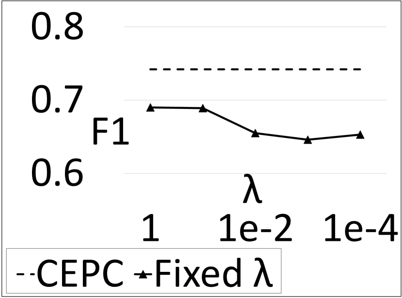
(a) CEPC vs. Fixed $\lambda$

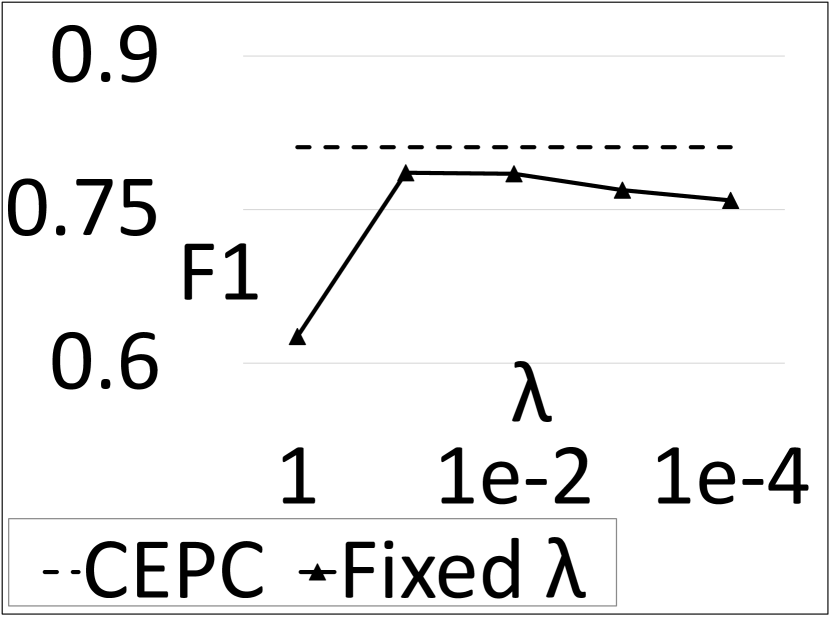
(b) CEPC vs. Fixed $\lambda$

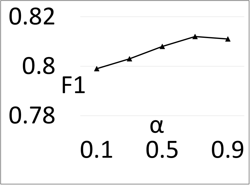
(c) F1 vs. $\alpha$

Figure 2: 2(a)-2(b)) CEPC in comparison with a model with fixed scale factor $\lambda$ (Equation 15), in Incident (2(a)) and Illness (2(b)) datasets. 2(c)) Model sensitivity to the penalty term $\alpha$ (Equation 15) in Illness dataset.

Dataset	Method	F1	Precision	Recall
Incident	Meta-Target	0.713	0.689	0.811
	CEPC	0.742	0.725	0.809
Illness	Meta-Target	0.799	0.762	0.845
	CEPC	0.811	0.786	0.841

Table 3: Using the source domains as meta-targets to tune for the scale factor $\lambda$ (Equation 15).

Method	F1	Precision	Recall
CEPC	0.811	0.786	0.841
CEPC w/o Paired Classifier	0.793	0.713	0.895
CEPC w/o Classifier Capacity	0.801	0.782	0.826
CEPC w/o Transformation Cost	0.809	0.783	0.839

Table 4: Ablation study of the paired classifiers (Sections 3.2, 3.3, and 3.4) in Illness dataset.

We also demonstrate whether pairing source classifiers (Section 3.2) is effective. Additionally, we show the extent in which the transformation costs (Section 3.3) and the classifier capacities (Section 3.4) contribute to the performance. To this end, we report an ablation study on these modules in Table 4. We see that this technique is indeed effective, and also each one of its underlying steps are contributing.

Finally, we report the sensitivity of CEPC to the hyper-parameter $\alpha$ in Figure 2(c) (Equation 15). We see that as the value of $\alpha$ increases, the performance slightly improves.

In this work we demonstrated that several domain adaptation models that previously have shown to be competitive, not necessarily perform well in user-generated data, specifically in social media data. Our experiments suggest that every area may have particular properties and call for further investigation into under-explored areas. Future work may evaluate the efficacy of existing models in languages other than English, specifically those that have lower resources and are richer in morphology, e.g., Persian and Kurdish.

6 Conclusions

In this work, we proposed a novel model for multiple-source unsupervised Domain Adaptation. Our model possesses two essential properties: 1) It can automatically coordinate domain encoders by inferring their update rates via a proxy task. 2) It can pair source classifiers based on their predicated error rates in the target domain. We carried out experiments in two datasets and showed that our model outperforms the state of the art.

References

- Alam et al. (2020) Alam, F.; Sajjad, H.; Imran, M.; and Ofli, F. 2020. Standardizing and Benchmarking Crisis-related Social Media Datasets for Humanitarian Information Processing. arXiv preprint arXiv:2004.06774.
- Ben-David et al. (2010) Ben-David, S.; Blitzer, J.; Crammer, K.; Kulesza, A.; Pereira, F.; and Vaughan, J. W. 2010. A theory of learning from different domains. Machine learning, 79(1-2): 151–175.
- Ben-David and Schuller (2003) Ben-David, S.; and Schuller, R. 2003. Exploiting Task Relatedness for Multiple Task Learning. In Schölkopf, B.; and Warmuth, M. K., eds., Learning Theory and Kernel Machines, 567–580. Berlin, Heidelberg: Springer Berlin Heidelberg.
- Biddle et al. (2020) Biddle, R.; Joshi, A.; Liu, S.; Paris, C.; and Xu, G. 2020. Leveraging Sentiment Distributions to Distinguish Figurative From Literal Health Reports on Twitter, 1217–1227. New York, NY, USA: Association for Computing Machinery. ISBN 9781450370233.
- Caruana (1997) Caruana, R. 1997. Multitask Learning. Mach. Learn., 28(1): 41–75.
- Cui and Bollegala (2020) Cui, X.; and Bollegala, D. 2020. Multi-source Attention for Unsupervised Domain Adaptation. arXiv preprint arXiv:2004.06608.
- Devlin et al. (2019) Devlin, J.; Chang, M.-W.; Lee, K.; and Toutanova, K. 2019. BERT: Pre-training of Deep Bidirectional Transformers for Language Understanding. In Proc of the 2019 NAACL, 4171–4186.
- Ganin and Lempitsky (2015) Ganin, Y.; and Lempitsky, V. S. 2015. Unsupervised Domain Adaptation by Backpropagation. In Bach, F. R.; and Blei, D. M., eds., Proceedings of the 32nd International Conference on Machine Learning, ICML 2015, Lille, France, 6-11 July 2015, volume 37 of JMLR Workshop and Conference Proceedings, 1180–1189. JMLR.org.
- Guo, Pasunuru, and Bansal (2020) Guo, H.; Pasunuru, R.; and Bansal, M. 2020. Multi-Source Domain Adaptation for Text Classification via DistanceNet-Bandits. In The Thirty-Fourth AAAI Conference on Artificial Intelligence, AAAI 2020, The Thirty-Second Innovative Applications of Artificial Intelligence Conference, IAAI 2020, The Tenth AAAI Symposium on Educational Advances in Artificial Intelligence, EAAI 2020, New York, NY, USA, February 7-12, 2020, 7830–7838. AAAI Press.
- Guo, Shah, and Barzilay (2018) Guo, J.; Shah, D. J.; and Barzilay, R. 2018. Multi-Source Domain Adaptation with Mixture of Experts. In Riloff, E.; Chiang, D.; Hockenmaier, J.; and Tsujii, J., eds., Proceedings of the 2018 Conference on Empirical Methods in Natural Language Processing, Brussels, Belgium, October 31 - November 4, 2018, 4694–4703. Association for Computational Linguistics.
- Haeusser et al. (2017) Haeusser, P.; Frerix, T.; Mordvintsev, A.; and Cremers, D. 2017. Associative Domain Adaptation. In Proceedings of the IEEE International Conference on Computer Vision (ICCV).
- Holzenberger, Blair-Stanek, and Van Durme (2020) Holzenberger, N.; Blair-Stanek, A.; and Van Durme, B. 2020. A Dataset for Statutory Reasoning in Tax Law Entailment and Question Answering. arXiv preprint arXiv:2005.05257.
- Isobe et al. (2021) Isobe, T.; Jia, X.; Chen, S.; He, J.; Shi, Y.; Liu, J.; Lu, H.; and Wang, S. 2021. Multi-Target Domain Adaptation With Collaborative Consistency Learning. In IEEE Conference on Computer Vision and Pattern Recognition, CVPR 2021, virtual, June 19-25, 2021, 8187–8196. Computer Vision Foundation / IEEE.
- Karisani and Karisani (2020) Karisani, N.; and Karisani, P. 2020. Mining coronavirus (covid-19) posts in social media. arXiv preprint arXiv:2004.06778.
- Karisani and Agichtein (2018) Karisani, P.; and Agichtein, E. 2018. Did You Just Have a Heart Attack?: Towards Robust Detection of Personal Health Mentions in Social Media. In Proc of the 2018 WWW, 137–146. ISBN 978-1-4503-5639-8.
- Karisani, Agichtein, and Ho (2020) Karisani, P.; Agichtein, E.; and Ho, J. 2020. Domain-Guided Task Decomposition with Self-Training for Detecting Personal Events in Social Media. In Proceedings of The Web Conference 2020, WWW ’20, 2411–2420. New York, NY, USA: Association for Computing Machinery.
- Karisani, Choi, and Xiong (2021) Karisani, P.; Choi, J. D.; and Xiong, L. 2021. View Distillation with Unlabeled Data for Extracting Adverse Drug Effects from User-Generated Data. arXiv:2105.11354.
- Karisani and Karisani (2021) Karisani, P.; and Karisani, N. 2021. Semi-Supervised Text Classification via Self-Pretraining. In Proceedings of the 14th ACM International Conference on Web Search and Data Mining, WSDM ’21, 40–48. Association for Computing Machinery.
- Karisani, Karisani, and Xiong (2021) Karisani, P.; Karisani, N.; and Xiong, L. 2021. Contextual Multi-View Query Learning for Short Text Classification in User-Generated Data. arXiv:2112.02611.
- Long et al. (2015) Long, M.; Cao, Y.; Wang, J.; and Jordan, M. I. 2015. Learning Transferable Features with Deep Adaptation Networks. In Bach, F. R.; and Blei, D. M., eds., Proceedings of the 32nd International Conference on Machine Learning, ICML 2015, Lille, France, 6-11 July 2015, volume 37 of JMLR Workshop and Conference Proceedings, 97–105. JMLR.org.
- Long et al. (2017) Long, M.; Zhu, H.; Wang, J.; and Jordan, M. I. 2017. Deep transfer learning with joint adaptation networks. In International conference on machine learning, 2208–2217. PMLR.