APEX at the QSO MUSEUM: Molecular gas reservoirs associated with $z\sim$3 quasars and their link to the extended Ly$\alpha$ emission

Abstract

Cool gas (T$\sim$10⁴ K) traced by hydrogen Ly$\alpha$ emission is now routinely detected around $z\sim 3$ quasars, but little is known about their molecular gas reservoirs. Here, we present an APEX spectroscopic survey of the CO(6-5), CO(7-6) and [Ci](2-1) emission lines for 9 quasars from the QSO MUSEUM survey which have similar UV luminosities, but very diverse Ly$\alpha$ nebulae. These observations ($\langle~{}\rm rms~{}\rangle=2.6$ mJy in 300 km s^-1) detected three CO(6-5) lines with 3.4$\leq I_{\rm CO(6-5)}\leq$5.1 Jy km s^-1, 620$\leq$FWHM$\leq$707 km s^-1, and three [Ci](2-1) lines with 2.3$\leq I_{\rm[C\textsc{i}](2-1)}\leq$15.7 Jy km s^-1, 329$\leq$FWHM$\leq$943 km s^-1. For the CO and [Ci] detected sources, we constrain the molecular gas reservoirs to be $\rm M_{H_{2}}=(0.4-6.9)\times 10^{11}M_{\odot}$, while the non-detections imply $\rm M_{H_{2}}<1.1\times 10^{11}M_{\odot}$. We compare our observations with the extended Ly$\alpha$ properties to understand the link between the cool and the molecular gas phases. We find large velocity shifts between the bulk of Ly$\alpha$ and the molecular gas systemic redshift in five sources (from $\sim$-400 to $\sim+$1200 km s^-1). The sources with the largest shifts have the largest Ly$\alpha$ line widths in the sample, suggesting more turbulent gas conditions and/or large-scale inflows/outflows around these quasars. We also find that the brightest ($I_{\rm[C\textsc{i}](2-1)}=15.7\pm 3.7~{}\rm Jy~{}km~{}s^{-1}$) and the widest (FWHM$\sim$900 km s^-1) lines are detected for the smallest and dimmest Ly$\alpha$ nebulae. From this, we speculate that host galaxy obscuration can play an important role in reducing the ionizing and Ly$\alpha$ photons able to escape to halo scales, and/or that these systems are hosted by more massive halos.

1 Introduction

Super-massive black holes are found at the centre of massive galaxies (e.g., Richstone et al. 1998; Ferrarese & Merritt 2000; Kauffmann & Haehnelt 2000; Kormendy & Ho 2013). They become visible as extremely luminous active galactic nuclei (AGN) through episodes of intense accretion across the history of the Universe (e.g., Schmidt 1963; Bañados et al. 2018; Lyke et al. 2020). Because of the large budget of rest-mass energy available, these objects can regulate their own growth and the evolution of their host galaxies, even if only a small fraction of their feedback couples efficiently to the surrounding material (e.g., Silk & Rees 1998; Di Matteo et al. 2005; Steinborn et al. 2015).

Within AGN, quasars are the most luminous sources where we can see the nuclear emission directly (e.g., Antonucci 1993; Elvis 2000). Clustering measurements suggest that quasars preferentially inhabit dark matter halos with masses $M_{\rm DM}\sim 10^{12}-10^{13}$ M_⊙ (e.g., Porciani et al. 2004; Shen et al. 2007; White et al. 2012; Timlin et al. 2018 and references therein). This mass range should guarantee that a non-negligible fraction of cool ($T\sim 10^{4}$ K) gas, inflowing from large intergalactic scales at redshifts $z\gtrsim 2$ does not shock heat at the halo boundary, but accretes in cold form (e.g., Dekel & Birnboim 2006). Quasars at such epochs are therefore expected to sit in halos with both a cool and a warm/hot gas ($T\sim 10^{5}-10^{7}$ K) phase (e.g., Kereš et al. 2005). Because the quasar number density peaks between $z\sim 2$ and $z\sim 3$ (e.g., Richards et al. 2006; Shen et al. 2020), these epochs ($\sim 10.4-11.6$  Gyr ago) are frequently targeted by observations to understand how quasars are triggered and which reservoirs, from halo to galaxy scales, sustain their central engines.

The halo gas, known as circumgalactic medium (CGM, e.g., Tumlinson et al. 2017), has been studied around quasars mostly targeting the cool phase both in absorption (e.g., Hennawi et al. 2006; Prochaska et al. 2013; Farina et al. 2013, 2014; Lau et al. 2018) and in emission (e.g., Heckman et al. 1991; Bunker et al. 2003; Hennawi & Prochaska 2013; Farina et al. 2019; Fossati et al. 2021). While the absorption technique usually relies on only one background sightline per foreground halo to provide statistical information on the physical properties of the CGM of quasars, studies of the CGM in emission are currently able to map the quasar CGM around individual systems. At $z\sim 2-3$, the study of projected quasar pairs has led to a number of new insights: (i) the measurement of the anisotropic clustering of H i systems around quasars (Hennawi & Prochaska 2007; Jalan et al. 2019) suggested that their ionizing radiation escapes anisotropically or intermittently, (ii) the discovery of large reservoirs ($>10^{10}$ M_⊙) of cool and metal-enriched ($Z\gtrsim 0.1$ Z_⊙) halo gas (Prochaska et al. 2013; Prochaska et al. 2014; Lau et al. 2016), and (iii) the study of the kinematics of the halo, which seems to suggest that the gas is in virial equilibrium with the dark matter halo, though there is some evidence for outflowing gas (Prochaska et al. 2014; Lau et al. 2018).

In recent years, sensitive integral field unit spectrographs like the Multi-Unit Spectroscopic Explorer (MUSE; Bacon et al. 2010), the Keck Cosmic Web Imager (KCWI; Morrissey et al. 2012) and the Palomar Cosmic Web Imager (PCWI; Matuszewski et al. 2010) revolutionized the study of CGM gas through emission lines by allowing deeper observations in reasonable amount of time. The seminal papers by Rees (1988) and Haiman & Rees (2001), predicted that gas surrounding quasars reprocesses the impinging strong UV radiation as Ly$\alpha$ emission. Current studies routinely report extended Ly$\alpha$ emission, with $\sim 200$ quasars surveyed to date at $2<z<4$ (e.g., Husband et al. 2015; Fumagalli et al. 2016; Borisova et al. 2016; Arrigoni Battaia et al. 2019a; Cai et al. 2019; O’Sullivan et al. 2020; Mackenzie et al. 2021; Fossati et al. 2021). The bulk of the extended emission traces gas on a few tens of kpc near the quasars, while large-scale structures extending to $R\gtrsim 80$ kpc are seen at lower surface brightness (SB${}_{\rm Ly\alpha}\sim 10^{-18}$ erg s^-1 cm^-2 arcsec^-2).

These studies reveal few extended structures over hundreds of kpc with SB${}_{\rm Ly\alpha}\gtrsim 10^{-17}$ erg s^-1 cm^-2 arcsec^-2 (Arrigoni Battaia et al. 2018a), likely pinpointing very dense environments (Hennawi et al. 2015, Nowotka et. al subm.). These rare and bright large-scale nebulae are also known as enormous Ly$\alpha$ nebulae (ELAN; Cai et al. 2017). The Ly$\alpha$ kinematics in the extended nebulae is consistent with gravitational motions in halos with masses consistent with typical quasar hosts (e.g., Arrigoni Battaia et al. 2019a; O’Sullivan et al. 2020), with a few exceptions with possible quasar winds extending over tens of kpc (Travascio et al. 2020).

While a large fraction of these Ly$\alpha$ nebulae are likely powered by the quasars, the balance between different plausible mechanisms is still debated. Most previous work assumes that the Ly$\alpha$ emission is due to recombination radiation following quasar photoionization (e.g., Heckman et al. 1991; Cantalupo et al. 2014). Resonant scattering of quasar Ly$\alpha$ photons and active companions can, however, provide a non-negligible contribution on scales of tens of kpc near compact sources (e.g., Cantalupo et al. 2014; Husemann et al. 2018; Arrigoni Battaia et al. 2019b). On top of this, there are large uncertainties on the ionizing radiation that impinges on the surrounding gas, because quasars are expected to be anisotropic, intermittent sources with different degrees of obscuration. These uncertainties hamper the physical interpretation of properties of the emitting gas (e.g., density $n_{\rm H}$, metallicity; Fossati et al. 2021).

There is, however, evidence in few systems that gas at large projected distances ($\gtrsim 50$ kpc) is not affected by resonant scattering effects, namely: (i) non-resonant lines follow the kinematics of the Ly$\alpha$ emission (e.g., He ii, Cai et al. 2017), and (ii) there is no evidence for double-peaked line profiles at the current resolution of the observational data (e.g., Arrigoni Battaia et al. 2018a). Neglecting resonant scattering, photoionization models match the observed Ly$\alpha$ and low HeII emission only if interstellar-medium-like densities ($n_{\rm h}\gtrsim 1$ cm^-3) in small-scale structures ($<20$ pc) are invoked (Cantalupo et al. 2014; Hennawi et al. 2015; Arrigoni Battaia et al. 2015; Borisova et al. 2016). This finding suggests the presence of dense CGM gas whose survival and entrainment in the warm/hot halo seem plausible from current high resolution “cloud-crushing” simulations(e.g., Gronke & Oh 2018, 2020; Kanjilal et al. 2021). Note that such processes are still largely unresolved by current cosmological simulations, even when attempts are made to resolve the CGM (e.g., Hummels et al. 2019; Peeples et al. 2019).

It is therefore of interest to ascertain observationally the maximum density the cool CGM gas is able to reach, and whether a fraction of the gas is able to transform into a molecular phase. The molecular gas around quasars can be best probed through different tracers depending on its physical properties (e.g., density, temperature) and those of the surrounding environment (e.g., radiation field) (e.g., Carilli & Walter 2013). Most previous works have focused on the rotational ($J$) transitions of carbon monoxide ¹²C¹⁶O (hereafter CO), which is the most abundant molecule after $\rm H_{2}$. Low-$J$ CO transitions are good tracers of the total cold molecular gas due to their low excitation temperatures. The CO($J$=1-0) ground transition requires an excitation temperature of only $\sim$5.5K (e.g., Bolatto et al. 2013). Using observations of different CO transitions and radiative transfer models (e.g., large velocity gradient, LVG; e.g., van der Tak et al. 2007), it is possible to constrain the CO spectral line energy distribution (SLED), and probe the excitation conditions and physical properties of the gas, as the density and kinetic temperature (e.g., Weiß et al. 2007b; Riechers et al. 2009).

The detection of CO emission in high-$z$ quasars greatly advanced thanks to the Atacama Large Millimeter/Submillimeter Array (ALMA, Wootten & Thompson 2009), and the Karl J. Jansky Very Large Array (JVLA, Perley et al. 2011). It is now possible to probe quasars at very high redshifts ($z\sim 6-7.5$, e.g., Wang et al. 2016; Venemans et al. 2017; Decarli et al. 2018; Novak et al. 2019). The population of z$\sim$3 quasars has also been studied in a number of previous studies(e.g., Weiß et al., 2007b; Schumacher et al., 2012; Carilli & Walter, 2013; Bischetti et al., 2021). From these works, we know that at these redshifts, the low CO transitions (i.e., $J\leq 3$) are expected to be faint, and that the redshifted CO lines lie at challenging frequencies for current and past instruments. Past CO observations of $z\sim 2-3$ quasars found molecular gas masses in the range of $\sim 10^{9}-10^{11}\ M_{\odot}$, similar to those found for quasars at higher redshift (e.g., Barvainis et al. 2002; Weiß et al. 2003; Beelen et al. 2004; Walter et al. 2011; Schumacher et al. 2012; Hill et al. 2019; Bischetti et al. 2021). These molecular reservoirs are characterized by densities of $\sim 10^{3.0}-10^{4.4}\rm cm^{-3}$ and kinetic temperatures of $\sim$30 - 90 K (Weiß et al., 2003; Weiss et al., 2007a; Schumacher et al., 2012), and, when resolved, have an effective radius of $\sim$ 0.5 - 2.5 kpc (e.g., Riechers et al., 2009; Schumacher et al., 2012; Stacey et al., 2021).

Currently, there is only tentative evidence for extended molecular gas reservoirs around individual quasars, but only few studies attempted long integrations. Riechers et al. (2006) presented CO(1-0) detections in three quasars at $z\sim 4$. Using single component LVG models, they found that all the flux detected in CO(1-0) was associated with the molecular gas traced by higher CO transitions. An extended component up to 30$\%$ of the total CO(1-0) luminosity was allowed by the observations. The extended component could have larger mass if the CO conversion factor was taken to be higher on larger scales. Emonts et al. 2019 targeted the CO(1-0) transition from the MAMMOTH-I ELAN located at $z\sim 2$ (Cai et al. 2017; Arrigoni Battaia et al. 2018b) and reported emission extended over tens of kpc, with roughly $50\%$ of the CO(1-0) emission outside of galaxies. Finally, Decarli et al. (2021) targeted the CO(3-2) transition for two $z\sim 2$ ELANe, the Slug (Cantalupo et al. 2014) and the Jackpot (Hennawi et al. 2015). Their NOEMA observations did not unveil any extended molecular reservoir in these objects down to molecular gas surface densities typical of starbursting systems ($\Sigma_{\rm H_{2}}<12-68$ M_⊙ pc^-2).

Fine structure lines of atomic carbon, for example [Ci], are an additional tracer to probe the cold molecular phase (e.g., Papadopoulos & Greve 2004; Valentino et al. 2018). Observational studies in the local Universe have shown that CO and [Ci] can coexist, suggesting that both transitions arise from the same regions (e.g., White et al. 1994; Ikeda et al. 2002; Israel & Baas 2002), though spatial variations could be present (e.g., Salak et al. 2019). Analysis using simultaneously [Ci] and multi-transition CO observations at high redshifts found agreement between the H₂ masses determined through the two different tracers (e.g., Weiß et al. 2003; Alaghband-Zadeh et al. 2013), corroborating the assumption that [Ci] and CO usually coexist (Carilli & Walter 2013). The carbon masses found in the literature for quasars at $z\sim 2-3$ are typically of the order of $10^{6}-10^{7}M_{\odot}$ and do not differ significantly from those found for quasars at $z>3$ (e.g., Weiß et al., 2003; Walter et al., 2011; Schumacher et al., 2012; Venemans et al., 2017; Banerji et al., 2018; Yang et al., 2019). Molecular masses are then usually obtained by assuming the same abundance of [Ci] relative to H₂ as found in high-z quasars (e.g., Weiß et al. 2005).

In this framework, we targeted the CO(6-5) ($\rm\nu_{rest}$ = 691.4731 GHz), CO(7-6) ($\rm\nu_{rest}$ = 806.6518 GHz) and [Ci] ³P₂-³P₁ (hereafter [Ci](2-1), $\rm\nu_{rest}$ = 809.3420 GHz) transitions with the SEPIA180 receiver (Belitsky et al. 2018b, a) on the Atacama Pathfinder Experiment (APEX) for a sample of nine z$\sim$3 quasars, whose halo gas has been studied in the QSO MUSEUM survey (Arrigoni Battaia et al., 2019a). With these observations, we aim to (i) constrain the molecular phase around these massive systems and thus start characterizing the multiphase nature of the halo gas, and (ii) investigate the relation between the molecular gas content and the large-scale cool phase. The molecular line detections also pin down the systemic redshift of the quasar very accurately, allowing us to probe the kinematics of the halo gas.

This work is structured as follows. In Section 2, we describe our sample, observations and data reduction. In Section 3 we present the observed line properties and refine the systemic redshift when possible. In Section 4, we describe the estimation of the molecular gas masses using different methods, and present results for these masses. In Section 5, we compare the derived molecular masses with the Ly$\alpha$ properties of our sources. In Section 6 we discuss our main results, and explore the link between the molecular gas content and the large scale Ly$\alpha$ emission. Finally, Section 7 summarizes our findings.

Throughout this paper, we adopt the cosmological parameter $H_{\rm 0}=70\ \rm km\ s^{-1}Mpc^{-1}$, $\Omega_{\rm M}=0.3$ and $\Omega_{\rm\Lambda}=0.7$.

2 Sample and observational data

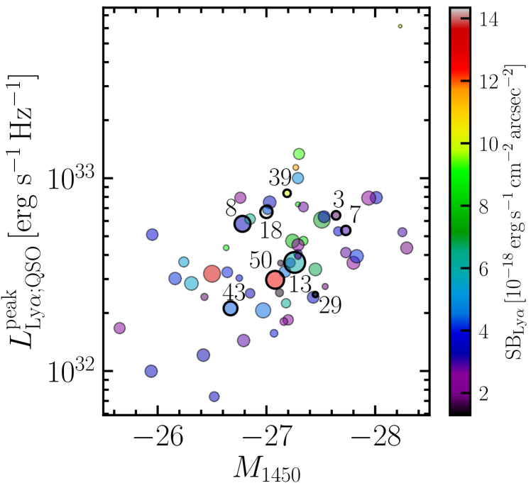
Figure 1: The peak specific luminosity at the Ly$\alpha$ line of the quasar versus $M_{\rm 1450\AA}$ for the QSO MUSEUM sample (Arrigoni Battaia et al. 2019a). The symbols sizes are proportional to the area of the Ly$\alpha$ nebulae, while the colours indicate their average Ly$\alpha$ surface brightness. We highlight the nine sources observed with APEX with black circles and their ID numbers.

Our sample is composed of nine quasars at $z\sim$3 selected from the QSO MUSEUM survey (Arrigoni Battaia et al., 2019a), which targeted 61 quasars with MUSE for the study of their CGM rest-frame UV line emission. The nine quasars were observed with the SEPIA180 receiver mounted on the APEX antenna, located in Llano de Chajnantor, Chile. The targets were selected using the following constraints:

• Visibility from the telescope site and the presence of CO rotational transitions, CO(6-5) and CO(7-6), and the [Ci](2-1) transition within the frequency range covered by the SEPIA180 instrument.

• The expected frequency of the targeted emission lines was required to be located far from the atmospheric 183 GHz water-absorption feature to best exploit the sensitivity of the SEPIA180 instrument, even under high water vapor conditions.

• Similar absolute magnitudes at rest frame 1450 Å, ranging between -27.64 and -26.67 mag, with a median of -27.20 (Figure 1).

• Coverage of a large portion of the physical parameter space of the QSO MUSEUM survey, namely Ly$\alpha$ nebulae with sizes spanning the range $\sim$29 - 467 arcsec² (or $\sim$1600 - 27000 kpc²) and surface brightnesses $\sim$1.25$\times$10^-18-1.43$\times$10^-17 erg s^-1 cm^-2 arcsec^-2 (Figure 1).

• One of the targets was selected to be radio-loud, reflecting a similar fraction of such objects in the parent quasar sample ($\sim$10$\%$, Ivezić et al. 2002).

The CO(6-5) ($\rm\nu_{obs}$ = 167.3 GHz) observations were carried out between October and December of 2018 under the ESO programme 0102.A-0394A (PI: F. Arrigoni Battaia), with a total of $\sim$133 hours of telescope time. The [Ci](2-1) ($\rm\nu_{obs}$ = 195.8 GHz) and CO(7-6) ($\rm\nu_{obs}$ = 195.2 GHz) observations were performed between May and December of 2019 under the ESO programme 0103.A-0306A (PI: F. Arrigoni Battaia), with a total of $\sim$140 hours of telescope time. The main beam full width half maximum (FWHM) of the SEPIA180 receiver is about $\sim$32” ($\sim$249 kpc) for the CO(6-5) observations and $\sim$ 30” ($\sim$234 kpc) for the [Ci](2-1) - CO(7-6) observations. Figure 2 shows Ly$\alpha$ images of the nine targets analysed in this work, with superimposed APEX beams shown as white circles. The acquired data will therefore provide an integrated spectrum of the emission within such beams. The median value of precipitable water vapor (PWV) was 1.4 and 1.5 mm for CO(6-5) and [Ci](2-1) - CO(7-6), respectively. The full histograms of the PWV values for the observations are shown in Fig. 3. A summary of the sample and observational setup is shown in Table 1. Due to source visibility and weather constraints, we obtained CO(6-5) data for 7 sources and [Ci](2-1) - CO(7-6) for 8 sources.

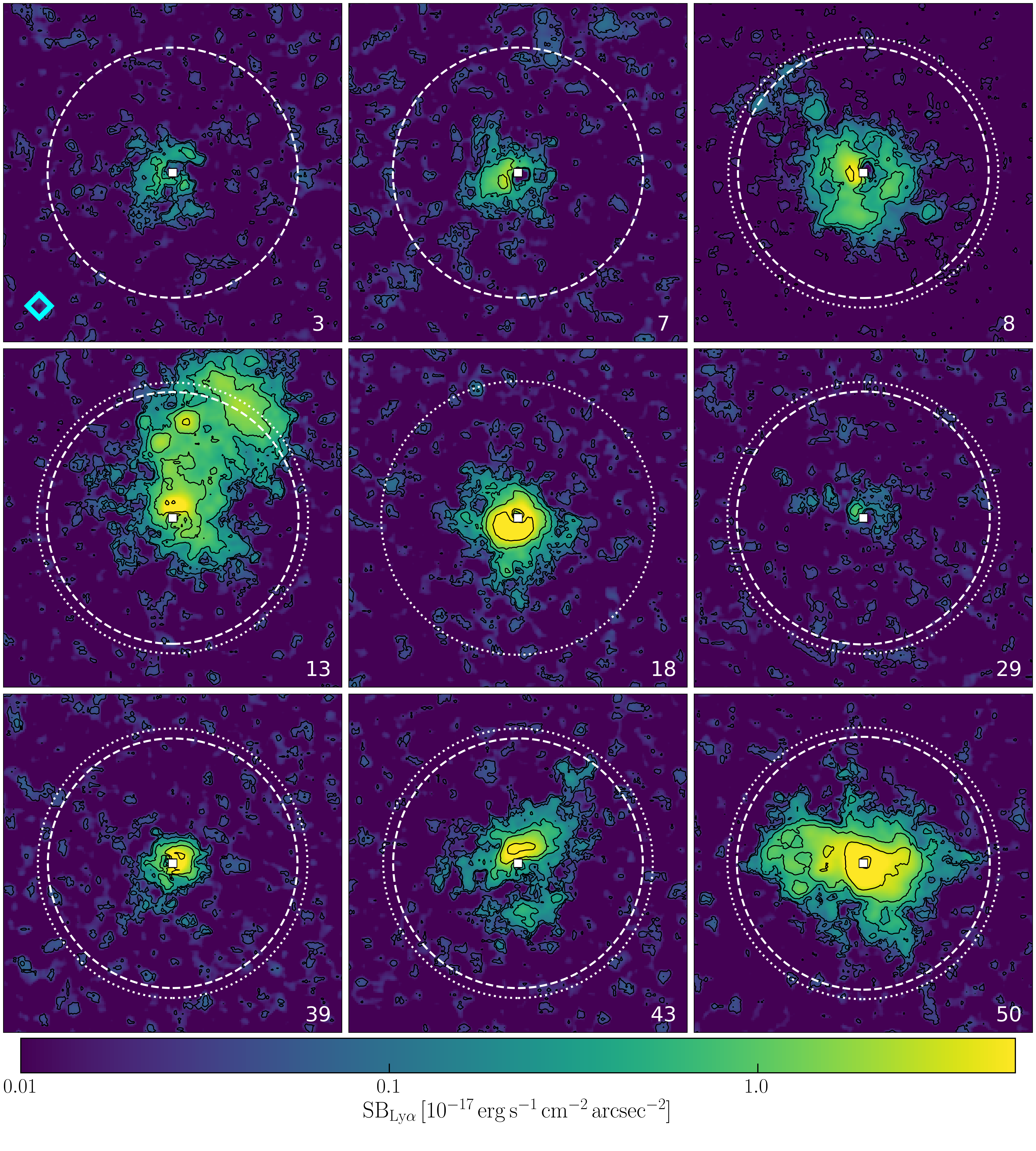
Figure 2: $40\arcsec\times 40\arcsec(\rm or\sim 312\ kpc\times 312\ kpc)$ MUSE Ly$\alpha$ surface brightness maps of the nebulae surrounding the 9 targets of this study (adapted from Arrigoni Battaia et al. 2019a). The numbers in the bottom right corner are the IDs from the QSO MUSEUM survey (see Table 1, first column). The white dotted circles represent the APEX/SEPIA180 beam sizes for the CO(6-5) observations ($\sim$32”), while the white dashed circles are the beam sizes for the [Ci](2-1) - CO(7-6) observations ($\sim$30”). The cyan diamond indicates that the source is radio-loud.

The data reduction was performed using the gildas/class package version 1.1. For each source the data corresponding to a different date were processed separately, before combining them. In this procedure, for every target the noisy edges ($\sim$3%) of the spectra were trimmed. Then, a velocity window was chosen to encompass the expected location of the emission line, according to the redshift of the source. First-degree polynomial baselines were computed neglecting the data within that window, and subtracted from the individual scans. All data for each source were then combined into one final spectrum, after visual inspection of individual scans. These spectra cover an average spectral window of $\sim$6000 km s^-1.

To further improve the root mean square (rms) of the final combined spectra, we applied the following procedure. For each target, we computed the rms for each used subscan in order to reject the nosiest data. We computed the median rms of the whole dataset (i.e., all dates for each source) and removed the data farthest away from this median. New reductions ignoring these subscans were performed following the steps described above, checking if the final rms of the dataset improved. We found that the removal of the noisiest subscans did not improve the final rms, because the decrease in exposure time compensates the improvement in rms, so we decided to keep all the data for the final reduction. The final rms for each tuning is reported in Table 1.

To illustrate the stability of the SEPIA180 instrument at the targeted frequencies, in Fig. 16 of Appendix A we show the rms as a function of the bin size (in km s^-1), for the final combined spectra of each source, starting from the original resolution and up to 600 km s^-1. At the bottom of each panel is shown by how much the observed rms deviates from the expected value. At a bin size of 300 km s^-1, we found a mild median deviation of 12$\%$ and 14$\%$ for the CO(6-5) and [Ci](2-1) - CO(7-6) observations, respectively.

As last step, we transformed the intensity units of the spectra, originally in temperature (K), to physical flux units. For this purpose, we assumed the conversion factor $38.4\pm 2.8$ Jy K^-1, calculated for the SEPIA180 receiver (Belitsky et al., 2018b).

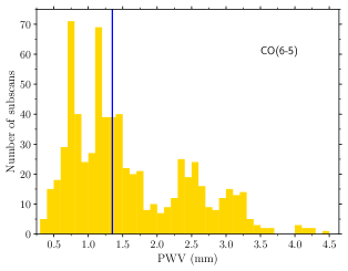
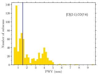
Figure 3: Histograms of the PWV values during the observations. Left panel: Values for the ESO programme 0102.A-0394A, the CO(6-5) observations. Right panel: Values for the ESO programme 0103.A-0306A, the [Ci](2-1) - CO(7-6) observations. The blue vertical lines indicate the median values.

Table 1: Sample, observations setup and log.

					0102.A-0394Aa				0103.A-0306Ab
IDc	Quasar	RA	DEC	z${}^{d}_{\rm sys}$	Frequencye	Exp. timef	RMSg	PWVh	Frequencye	Exp. timef	RMSg	PWVh
		(J2000)	(J2000)		(GHz)	(hr)	(mK)	(mm)	(GHz)	(hr)	(mK)	(mm)
3	J 0525-233	05:25:06.500	-23:38:10.00	3.110	-	-	-	-	196.000	4.8	0.131	3.6
7	SDSS J1209+1138	12:09:18.000	+11:38:31.00	3.117	-	-	-	-	195.932	5.4	0.086	1.8
8	UM683	03:36:26.900	-20:19:39.00	3.132	167.346	6.1	0.034	1.9	195.221	5.8	0.079	1.4
13	PKS-1017+109	10:20:10.000	+10:40:02.00	3.164	166.060	6.2	0.075	1.0	193.720	4.7	0.087	3.6
18	SDSS J1557+1540	15:57:43.300	+15:40:20.00	3.265	162.127	11.6	0.047	1.8	-	-	-	-
29	Q-0115-30	01:17:34.000	-29:46:29.00	3.180	164.600	11.5	0.060	1.5	192.000	13.6	0.065	1.7
39	SDSS J0100+2105	01:00:27.661	+21:05:41.57	3.100	168.000	8.1	0.071	1.7	196.888	6.0	0.047	2.1
43	CTSH22.05	01:48:18.130	-53:27:02.00	3.087	168.000	12.7	0.049	1.8	196.800	15.8	0.045	2.3
50	SDSS J0819+0823	08:19:40.580	+08:23:57.98	3.197	164.754	10.5	0.057	1.8	192.197	8.9	0.073	2.6

• ESO programme corresponding to the CO(6-5) observations.

• ESO programme corresponding to the [Ci](2-1) CO(7-6) observations.

• Identification number taken from the QSO MUSEUM survey (Arrigoni Battaia et al., 2019a).

• Quasar systemic redshift taken from the QSO MUSEUM survey (Arrigoni Battaia et al., 2019a), which has an intrinsic uncertainties of 415 km s^-1. See Table 3 for updated systemic redshifts ($z_{\rm mol,sys}$) calculated from the lines detected in this work.

• Tuning frequency used for the observations.

• Total ON-OFF exposure time per source. The total telescope time is roughly double this integration time.

• RMS per bin of 300 km s^-1 of the final combined spectrum, in antenna temperature $T^{*}_{A}$ units.

• Median PWV between all the observed dates for each source.

3 Observational results

The resulting APEX spectra, reduced and converted to flux density units (mJy), are presented in Figs. 4 and 5 for the CO(6-5) and [Ci](2-1)-CO(7-6) observations, respectively. For all sources, the left panel spectrum has a bin size between 150 and 200 km s^-1 (depending on the depth of the data), and the right panel spectrum has a bin size of 300 km s^-1. These two different bin sizes are shown to highlight the reliability of the detections. In this work we report as detections the lines that fulfill the following conditions: i) have a peak emission at S/N$>2\sigma$, at bin sizes of 300 km s^-1, ii) are also present at the resolution of 150 km s^-1 but with lower significance than at 300 km s^-1, and consistent integrated fluxes, iii) have an integrated S/N$>3\sigma$. In Appendix B we show that this detection algorithm is reliable, giving basically a zero-rate of false positive identifications in a negative and jack-knife tests.

Importantly, throughout this work we assume that the detected emission is due to the central quasar hosts, unless specified. We checked this assumption by computing the number of expected line-emitter companions for each transition within the APEX observations, down to the $3\sigma$ limiting luminosities of $L^{\prime}$=3.13$\times 10^{10}$, 3.02$\times 10^{10}$ and 2.65$\times 10^{10}$ K km s^-1 pc², respectively for CO(6-5), CO(7-6), and [Ci](2-1). Specifically, we assumed (i) a cylindrical volume defined by the APEX primary beam and the covered velocity range of $\sim 6000$ km s^-1, (ii) the luminosity function of CO(6-5), CO(7-6) and [Ci](2-1) emission measured for similar redshifts ($z\sim 2$; Decarli et al. 2020), and (iii) a deterministic bias model for the clustering of sources around quasars (e.g., García-Vergara et al. 2017; García-Vergara et al. 2019). In this model, we assume a power-law shape for the clustering, with a fixed slope of $\gamma=1.8$, and we use the $z\sim 3$ quasar clustering (Shen et al. 2007) and the clustering of Lyman-break galaxies (LBGs) at $z=4$ (Ouchi et al., 2004), which are assumed to have similar clustering as CO and [Ci] sources.

Following these assumptions, we found that the expected number of companions for the total number of observed fields per line (7, 8, 8) are 0.07, 0.01, 1.39, respectively for CO(6-5), CO(7-6), and [Ci](2-1). We caution that the luminosity functions in Decarli et al. (2020) are still associated with large uncertainties, and only upper limits are reported at the bright-end sampled by our observations. We have thus extrapolated their measurements up to brighter fluxes, and therefore our estimations represent upper limits for the number of expected companions. Specifically, the worst case is the current [Ci](2-1) luminosity function, which has a relatively flat shape (see Fig. 7 of Decarli et al. 2020). In this case, our extrapolation is flat and therefore represents a clear upper limit considering that the luminosity function is expected to steeply decrease for high luminosities. In summary, the only transition for which we may find a companion is [Ci](2-1), with a conservative probability $<17$% for each field. Follow-up high-resolution observations with interferometers (e.g., ALMA, NOEMA) are required to verify this assumption and assess whether any of the detected emission comes from companions and/or larger scales.

We also computed the probability that one detected line in one field is actually any CO or [Ci] transition from an interloper galaxy at possible lower redshifts given our tunings, by assuming the luminosity functions in Decarli et al. (2019, 2020), and the comoving volume spanned by our observations. Once again, these estimates represent upper limits as our observations sample the bright-end of the luminosity functions. We found that the probability of observing a contaminant is <0.2% for any CO or [Ci] line. Therefore, it is very likely that any detected emission in our observations is associated with the quasar or its environment.

3.1 Emission line measurements

We measured the molecular velocity-integrated emission line fluxes $I_{\rm CO(6-5)}$, $I_{\rm[C{\textsc{i}}](2-1)}$ and I_CO(7-6), by fitting Gaussian to the detected lines. For those spectra that presented two peaks, a double Gaussian fit was applied. The uncertainties of the measured fluxes include the aforementioned error on the flux conversion factor. The Gaussian fits also provided an estimate of the full width at half maximum (FWHM) of the emission lines and their respective uncertainties.

When an emission line was not detected, we derived 3$\sigma$ upper limits using the rms noise within the same velocity range for the emission lines that were detected for that target, and within a velocity width of 300 km s^-1 (expected average line width for quasar hosts, e.g., Weiß et al. 2003; Weiss et al. 2007a; Walter et al. 2011) when no line was detected. In Table 2 we tabulate these fluxes (or upper limits), FWHM and their respective uncertainties for each source.

For the quasars with IDs 39 ([Ci](2-1) line) and 43 (CO(6-5) line), it was not possible to obtain a good Gaussian fit at bin sizes of 300 km s^-1 (see Figs. 4 and 5). Therefore, their integrated fluxes were first estimated by adding the area covered by each bin of 300 km s^-1 contained within the emission line and verified against a Gaussian fit at bin sizes between 150 and 200 km s^-1. Their integrated fluxes computed from both bin sizes are consistent, as per our detection criteria. The FWHMs and fluxes given in Table 2 are those estimated with the Gaussian fit. For the quasar with ID 3 (or J 0525-233), all line properties are listed using bin sizes of 150 km s^-1, because at this resolution we obtained a better fit (see Fig. 5) than at bin sizes of 300 km s^-1.

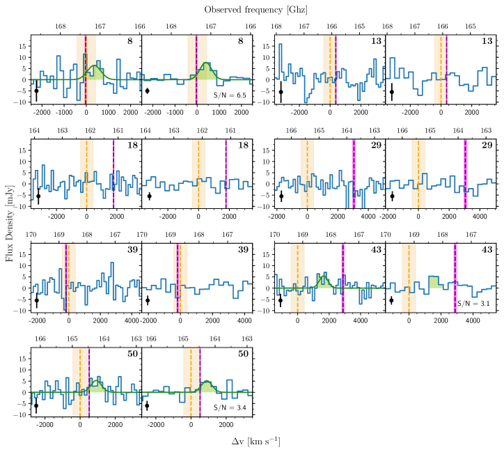
Figure 4: The seven APEX CO(6-5) spectral line observations. Each observed spectrum is shown with bin sizes between 150 and 200 km s^-1 (left column) and 300 km s^-1 right (column). In each panel, the vertical black error bar represents the uncertainty (rms) per bin, while the ID number of each quasar is shown in the top right corner. The orange vertical lines at the velocity zero point represent the systemic redshift of the sources before our APEX observations (from Civ, see section 3.2), and the shaded regions correspond to its uncertainty ($\sim$415 km s^-1, Arrigoni Battaia et al. 2019a). The purple vertical lines represent the nebulae Ly$\alpha$ redshift from MUSE extracted within the APEX beam (see Fig. 2), with their corresponding uncertainty (magenta shaded regions). The green shaded area indicates the detected CO(6-5) emission line, while the dark green curve represents the Gaussian fit applied to this line, when possible.

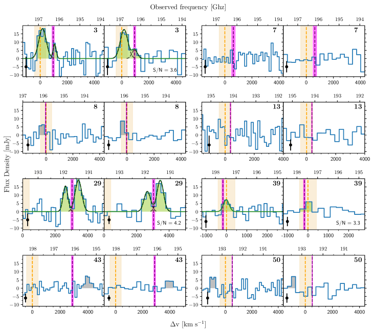
Figure 5: Same as Figure 4, but for the eight APEX CO(7-6)-[Ci](2-1) spectral line observations. Here, the zero velocities are placed at the expected [Ci](2-1) transition, considering the systemic redshift from Civ (orange vertical line) with its uncertainty (shaded region) (see section 3.2). The grey shaded areas indicate a likely spurious source (ID8, see section 3.1 and Appendix B) or tentative features (IDs 43 and 50) that do not belong to the quasar hosts. For sources with IDs 3 and 29, we applied a double Gaussian fit, where the black dashed lines represent the single Gaussian components. For ID 3, a second component was added not to overestimate the integrated flux of the [Ci](2-1) line. The emission lines of quasar with ID 29 are both due to [Ci](2-1) (see section 3.1), and its systemic redshift (orange line) lies outside the plotted window.

Table 2: CO(6-5), [Ci](2-1), CO(7-6) fluxes, FWHM, and integrated S/N ratios.

ID	Quasar	ICO(6-5)	S/NCO(6-5)	FWHMCO(6-5)	ICI(2-1)	S/NCI(2-1)	FWHMCI(2-1)	ICO(7-6)	S/NCO(7-6)	FWHMCO(7-6)
		(Jy km s-1)		(km s-1)	(Jy km s-1)		(km s-1)	(Jy km s-1)		(km s-1)
3	J 0525-233	-	-	-	12.4$\pm$3.4†	3.6	640$\pm$168†	<6.6 (2.4$\pm$1.9†∗)	- (1.3†∗)	- (265$\pm$217†∗)
7	SDSS J1209+1138	-	-	-	<3.1	-	-	<3.1	-	-
8	UM683	5.1$\pm$0.8	6.5	620$\pm$175	<3.9	-	-	<3.9	-	-
13	PKS-1017+109	<2.6	-	-	<3.0	-	-	<3.0	-	-
18	SDSS J1557+1540	<1.6	-	-	-	-	-	-	-	-
29	Q-0115-30	<3.6	-	-	15.7$\pm$3.7‡	4.2	943$\pm$249‡	<4.0	-	-
39	SDSS J0100+2105	<2.0	-	-	2.3$\pm$0.7†	3.3	329$\pm$109†	<1.7	-	-
43	CTSH22.05	3.4$\pm$1.1†	3.1	643$\pm$279†	<2.3	-	-	<2.3	-	-
50	SDSS J0819+0823	3.9$\pm$1.1	3.4	707$\pm$100	<3.9	-	-	<3.9	-	-

• Note: The integrated fluxes, S/N and FWHM have been calculated using a bin size of 300 km s^-1. For the cases with non-detections, 3$\sigma$ upper limits on the fluxes are provided.

• Feature added in the Gaussian fit of quasar with ID 3 (or J 0525-233), to not overestimate the integrated flux of the [Ci](2-1) line at bin size of 300 km s^-1 (see Fig. 5).

• These values have been calculated using a bin size between 150 and 200 km s^-1.

• These values have been calculated as the sum of the two Gaussian components (see Fig. 5). For each component, the individual values of I_CI(2-1) are 6.1$\pm$2.9 km s^-1 and 9.5$\pm$2.3 Jy km s^-1, with FWHM_CI(2-1) values of 471$\pm$224 km s^-1 and 471$\pm$108 km s^-1, respectively.

We started the analysis from the CO(6-5) tuning. From the spectra shown in Fig. 4, we found CO(6-5) emission line detections (represented by a green shaded area) for three sources: quasars with IDs 8, 43, and 50. Two of these detections are closer to the redshift of the Ly$\alpha$ nebula (IDs 43 and 50; purple vertical line) than the uncertain systemic redshift computed from Civ (orange vertical line). They present fluxes of 3.4$\leq I_{\rm CO(6-5)}$<5.1 Jy km s^-1. The other targeted sources, quasars with IDs 13, 18, 29 and 39, do not present any CO(6-5) emission down to the current rms. We therefore report 3$\sigma$ upper limits for these sources (see Table 2).

From the spectra in Fig. 5, we found [Ci](2-1) emission line detections in quasars with IDs 3, 29, and 39. They have fluxes of 2.3$\leq I_{\rm[C\textsc{i}](2-1)}\leq$15.7 Jy km s^-1. The quasar with ID 8 (or UM683) has a feature at 196.1 GHz (or -328 km s^-1, integrated S/N = 3.1, $I_{\rm line}\sim$3 Jy km s^-1, which could be a spurious line given the results of the jack-knife test for this spectrum (see Appendix B). For completeness, we also report that the quasars with ID 43 (or CTSH22.05) and ID 50 (or SDSS J0819+0823) have tentative features at 195.4 GHz (or +3966 km s^-1, integrated S/N = 2.7, $I_{\rm line}\sim$2.8 Jy km s^-1) and 193.4 GHz (or -957 km s^-1, integrated S/N = 2.1, $I_{\rm line}\sim$2.5 Jy km s^-1), respectively. The redshift of these lines is not consistent with the CO(6-5) detections for these sources, but they might be an associated object. We note that sub-millimeter galaxies (SMG) have often being found in the surroundings of quasars (e.g., Silva et al. 2015), however the CO(6-5) transition (detected for IDs 43 and 50) is expected to be stronger in quasars than in SMG (Carilli & Walter, 2013). Also, we stress that the detections in the CO(6-5) tuning must come from the quasar, due to the low probability of finding a companion in this transition in our observations (see Section 3). The rest of the sources do not have any detected emission lines at the rms of the current observations.

It is important to stress that we considered our detected lines as [Ci](2-1) and not CO(7-6) because they are closer to the expected position of [Ci](2-1) based on the systemic redshift of the sources (within 1$\sigma$, IDs 3 and 39), or because if they were CO(7-6) emission, CO(6-5) detections would be also expected unless unphysical line ratios are assumed (quasar with ID 29, see next paragraph). We acknowledge that the used systemic redshifts (based on Civ) are uncertain (see Section 3.2) and further data are needed to verify our line identifications.

The spectrum of the quasar with ID 3 (or J 0525-233) shows the [Ci](2-1) emission line (at 196.8 GHz) and a S/N = 1.4 bump (binning of 300 km s^-1) at the expected location of CO(7-6) (196.2 GHz), which we estimate would contribute $\sim 20$% of the [Ci](2-1) flux when using the 300 km s^-1 binning. In contrast, the quasar with ID 29 (or Q-0115-30) presents two emission lines (at 191.9 and 191.4 GHz) consistent with the redshift of its Ly$\alpha$ nebula. Both these lines likely correspond to [Ci](2-1). To confirm this, we first assumed that the line at frequency 191.4 GHz was CO(7-6) and estimated the observed I_CO(7-6)/I_CO(6-5) ratio ($>3.73$). We then compared this observed ratio to theoretical predictions from large velocity gradient (LVG) models (Goldreich & Kwan, 1974) with different physically plausible kinetic temperatures and densities (see Section 4.2 for a detailed explanation of these models and input parameters). This test did not allowed us to find any modelled I_CO(7-6)/I_CO(6-5) ratio as high as that observed, indicating that the line peak at lower frequencies also corresponds to [Ci](2-1). We stress that this identification needs further confirmation, e.g. by targeting additional transitions from this source. Quasar ID 29, with a total $I_{\rm[C{\textsc{i}}](2-1)}=15.7\pm 3.7$ Jy km s^-1, is therefore the brightest [Ci](2-1) detection in this sample. Furthermore, it is $\sim$3 times brighter than the lensed Cloverleaf quasar ($I_{\rm[C{\textsc{i}}](2-1)}\sim~{}5.2$ Jy km s^-1,Weiß et al. 2003), which is as far as we know the brightest [Ci](2-1) $z\sim 3$ quasar detected in the literature. We further discuss the nature of this double-peak emission of quasar with ID 29 (or Q-0115-30) in Section 6.1.2.

Overall, our observations suggest that [Ci](2-1) is stronger than CO(7-6) in these $z\sim 3$ quasars. This is in contrast with other observations of the same transitions in different $z\sim 4-7$ quasars (Riechers et al. 2009; Venemans et al. 2017; Lu et al. 2018; Wang et al. 2019; Yang et al. 2019) and $z\sim$ 2.5-3 quasars (Weiß et al., 2003; Walter et al., 2011; Schumacher et al., 2012), likely indicating that the excitation conditions in the molecular gas are different. Also, Banerji et al. (2018) observed these transitions in two quasars and their companions at $z\sim 2.5$, finding a [Ci](2-1) line slightly stronger than CO(7-6) in one quasar and one companion. To our knowledge, the studies mentioned above are the only available observations of these lines in the literature. Therefore, if our observations are confirmed in deeper datasets, current literature could be affected by low number statistics. We further note that [Ci](2-1) is stronger than CO(7-6) in high-redshift radio galaxies ($\sim$5 times stronger, e.g., Gullberg et al. 2016), which can be explained as enhancement of atomic carbon in cosmic ray dominated regions (e.g., Bisbas et al., 2017).

3.2 Redshifts from molecular lines

A precise estimate of the systemic redshifts of quasars plays a fundamental role in understanding the physical processes and kinematics of each system. For instance, an accurate systemic redshift would allow us to better constrain the cool gas kinematics mapped on large scales by the Ly$\alpha$ emission, and to compare it to cosmological simulations (Arrigoni Battaia et al., 2019a).

The uncertain systemic redshifts for our sample, estimated by Arrigoni Battaia et al. (2019a), are shown in the fifth column of Table 1. These redshifts were determined from the peak of the Civ line, after correcting from the expected luminosity-dependent blue-shift (Shen et al., 2016), and have an intrinsic uncertainty of 415 km s^-1. This large uncertainty, comparable to outflow/inflow velocities expected in quasar halos, hampers any kinematical study of these systems. However, the molecular emission lines should provide a more robust measure of the quasar’s systemic redshift (e.g., Banerji et al. 2017; Bischetti et al. 2021). We therefore derived new systemic redshifts for the objects with detected molecular lines. For the case of ID 29, the redshift was estimated as an average between the centroids of the two peaks. These new redshifts and their uncertainties are listed in Table 3. They have on average an uncertainty of 74.8 km s^-1 and a difference of $+$1045 km s^-1 (or $\Delta z=+0.014$) with respect to the systemic redshifts from Civ (see also Section 5.2). Hereafter we will assume these new values as systemic redshifts.

Table 3: Redshifts and central frequencies obtained from the targeted molecular lines, and velocity shifts from the large-scale Ly$\alpha$ emission within the same APEX aperture.

ID	Quasar	z${}^{a}_{\rm CO(6-5)}$	$\nu_{\rm CO(6-5)}$	z${}^{b}_{\rm C\textsc{i}(2-1)}$	$\nu_{\rm C\textsc{i}(2-1)}$	z${}^{c}_{\rm CO(7-6)}$	$\nu_{\rm CO(7-6)}$	z${}^{d}_{\rm mol,sys}$	$\Delta v^{e}_{\rm Ly\alpha Neb-mol}$	FHWMLyα
			(GHz)		(GHz)		(GHz)		(km s-1)	(km s-1)
3	J 0525-233	-	-	3.112$\pm$0.001	196.81$\pm$0.05	- (3.111$\pm$0.001)	- (196.17$\pm$0.06)	3.112$\pm$0.001	786$\pm$109	1542$\pm$196
7	SDSS J1209+1138	-	-	-	-	-	-	-	-	-
8	UM683	3.137$\pm$0.001	167.13$\pm$0.04	-	-	-	-	3.137$\pm$0.001	-423$\pm$76	915$\pm$46
13	PKS-1017+109	-	-	-	-	-	-	-	-	-
18	SDSS J1557+1540	-	-	-	-	-	-	-	-	-
29	Q-0115-30	-	-	3.223$\pm$0.001‡	191.65$\pm$0.06‡	-	-	3.223$\pm$0.001	-11$\pm$120	508$\pm$172
39	SDSS J0100+2105	-		3.100$\pm$0.001	197.42$\pm$0.03	-	-	3.100$\pm$0.001	-152$\pm$64	781$\pm$100
43	CTSH22.05	3.110$\pm$0.002	168.26$\pm$0.07	-	-	-	-	3.110$\pm$0.002	1236$\pm$133	1068$\pm$142
50	SDSS J0819+0823	3.210$\pm$0.001	164.26$\pm$0.02	-	-	-	-	3.210$\pm$0.001	-377$\pm$44	967$\pm$38

• Redshift obtained from the observed CO(6-5) emission line.

• Redshift obtained from the observed [Ci](2-1) emission line.

• Redshift obtained from the observed CO(7-6) emission line.

• Quasar systemic redshift estimated using the observed molecular lines.

• Velocity shift between the Ly$\alpha$ line peak of the nebulosities (extracted within the APEX beam, see Fig. 2) and the systemic redshift $z_{\rm mol,sys}$.

• These values have been calculated as the average between the two Gaussian components (see Fig. 5). For each component, the individual values of $\nu_{\rm C\textsc{i}(2-1)}$ are 191.91$\pm$0.11 GHz and 191.39$\pm$0.06 GHz.

4 Molecular mass estimates

In this section we estimate molecular gas masses $\rm M_{H_{2}}$ by using different methods. Specifically, we compute i) carbon masses $\rm M_{\rm C{\textsc{i}}}$ and derive the respective $\rm M_{H_{2}}$ by assuming a carbon abundance relative to H₂, ii) $\rm M_{H_{2}}$ for sources that have a measured constraint (upper limit) on the CO(7-6)/CO(6-5) ratio, iii) $\rm M_{H_{2}}$ by combining the two previously obtained mass ranges from [Ci] and the CO ratio, and iv) $\rm M_{H_{2}}$ for sources with no clear constraint on the CO ratio (i.e. sources with non-detections).

4.1 Atomic carbon mass

The mass of the atomic carbon can be estimated from the [Ci](2-1) line luminosity through the formulation presented in Weiß et al. (2003, 2005), under the assumption that this [Ci] transition is optically thin:

$$\frac{M_{\rm C{\textsc{i}}}}{M_{\odot}}=4.566\times 10^{-4}Q(T_{\rm ex})\frac{1}{5}e^{T_{\rm 2}/T_{\rm ex}}L^{\prime}_{\rm[C{\sc I}]}$$ (1)

where $Q(T_{\rm ex}$) = 1+3$e^{-T_{1}/T_{\rm ex}}$+5$e^{-T_{2}/T_{\rm ex}}$ corresponds to the Ci partition function, $T_{\rm ex}$ is the excitation temperature, and $T_{1}$ = 23.6 K and $T_{2}$ = 62.5 K correspond to the energies above the ground state. We used $T_{\rm ex}$=30 K as frequently found in high-redshift quasars (e.g., Weiß et al. 2003; Walter et al. 2011). The [Ci] line luminosity, $L^{\prime}_{\rm[C{\sc I}]}$, can be estimated via (Solomon et al., 1992)

$$L^{\prime}_{\rm line}=3.25\times 10^{7}I_{\rm line}\nu_{\rm obs}^{-2}D_{\rm L}^{2}(1+z)^{-3}$$ (2)

where $I_{\rm line}$ is the velocity-integrated line flux in units of Jy km s^-1, $\nu_{\rm obs}$ is the observed frequency in units of GHz, and $D_{\rm L}$ corresponds to the luminosity distance in Mpc. The final units of $L^{\prime}_{\rm line}$ are K km s^-1 pc².

As noted in Section 3.1, the [Ci](2-1) emission line is detected for three sources of our sample: quasars with IDs 3, 29 and 39. Using equation 1, we found atomic carbon masses in the range of $\sim$4.0$\times$10⁷M_⊙ - 3.1$\times$10⁸M_⊙. For the five sources with upper limits on the [Ci](2-1) transition (quasars with IDs 7, 8, 13, 43 and 50), we found atomic carbon masses < 8.0$\times$10⁷M_⊙. The detected sources show higher values than usually reported for quasars in the literature. Indeed, it is common to find values of the order 10⁶ - 10⁷M_⊙, when the same excitation temperature of 30 K is assumed (e.g., Walter et al., 2011; Venemans et al., 2017; Yang et al., 2019). The value for each source is listed in the third column of Table 4. It is important to note that the assumption of a higher $T_{\rm ex}$ in equation 1, for instance $T_{\rm ex}$=50 K, implies a $M_{\rm C{\textsc{i}}}$ $\sim$38 $\%$ lower.

The atomic carbon mass can be used to determine the molecular gas mass using the atomic carbon abundance relative to H₂:

$$\frac{X[\rm C{\textsc{i}}]}{X[\rm H_{2}]}=\frac{M_{\rm C{\textsc{i}}}}{6M_{\rm H_{2}}}.$$ (3)

In this work we assumed $X[\rm C{\textsc{i}}]/X[\rm H_{2}]$= (8.4 $\pm$ 3.5) $\times$10^-5 as usually done in the literature for high-redshift quasars (e.g., Walter et al. 2011; Venemans et al. 2017). We note that this value is higher than what has been recently found for $z\sim 1-3$ main sequence galaxies ($\sim$1.7$\times$10^-5, Valentino et al. 2018; Boogaard et al. 2020).

Using this method, we constrained molecular gas masses for quasars with IDs 3, 29 and 39, which span from $\sim$8.0$\times$10¹⁰M_⊙ to $\sim$6.1$\times$10¹¹M_⊙. For quasars with IDs 7, 8, 13, 43 and 50, we found molecular gas masses < 1.5$\times$10¹¹M_⊙. Most of these molecular gas masses are higher than the typical range ($\sim$10⁹-10¹¹M_⊙) found in the literature for other high-$z$ quasars (e.g., Weiß et al., 2003; Walter et al., 2011; Anh et al., 2013; Hill et al., 2019). We list all these values in the fourth column of Table 4.

Importantly, we are assuming that all the [Ci](2-1) emission comes from the quasar hosts. If part of this emission comes from larger areas, the $T_{\rm ex}$ might break into different values (e.g., lower/higher on larger/smaller scales), affecting the molecular masses estimated in this work. To constraint $T_{\rm ex}$ around these quasars, resolved [Ci](2-1) and [Ci](1-0) observations are needed (e.g., ALMA, NOEMA).

Table 4: Molecular, carbon and dynamical mass estimations.

ID	Quasar	M$\rm{}_{C\textsc{i}}$ a	M$\rm{}_{H_{2}}$ b	M$\rm{}_{H_{2}}$ c	M$\rm{}_{H_{2}}$ d	M${}_{\rm dyn}{\rm sin}^{2}(i)$ e
		(108M⊙)	(1011M⊙)	(1011M⊙)	(1011M⊙)	(1011M⊙)
3	J 0525-233	2.3$\pm$0.6	4.6$\pm$2.3	<6.9	2.3-6.9∗	1.6$\pm$0.8
7	SDSS J1209+1138	<0.6	<1.1	<3.2	<1.1	-
8	UM683	<0.7	<1.5	0.7-64.1	0.7-1.5	1.5$\pm$0.8
13	PKS-1017+109	<0.6	<1.1	<3.2	<1.1	-
18	SDSS J1557+1540	-	-	<0.6	<0.6	-
29	Q-0115-30	3.1$\pm$0.7	6.1$\pm$2.9	<4.4	3.2-4.4	4.4$\pm$1.0 ‡
						12.4$\pm$6.6 ⋄
39	SDSS J0100+2105	0.4$\pm$0.1	0.8$\pm$0.4	<1.8	0.4-1.8†	0.4$\pm$0.3
43	CTSH22.05	<0.4	<0.9	0.5-42.7	0.5-0.9	1.6$\pm$1.4
50	SDSS J0819+0823	<0.8	<1.5	0.5-51.3	0.5-1.5	1.9$\pm$0.6

• Note: Upper limits of masses provided in each column are due to non-detections of [Ci] and/or CO (see Section 4).

• Atomic carbon mass assuming an excitation temperature of 30 K (see Section 4.1).

• Molecular gas mass derived from the atomic carbon mass (see Section 4.1, equation 3).

• Molecular gas mass derived from CO (see Section 4.2).

• Molecular gas mass derived from applying both CO and [Ci] constraints (see Section 4.3).

• Inclination-dependent dynamical masses (see Section 6.1.1). The reported uncertainties include only the errors on the FWHM values.

• In the case the detected line for ID 3 is CO(7-6), we estimate $1.2<M_{\rm H_{2}}/[10^{11}{\rm M_{\odot}}]<4.5$ from the final CO SLEDs (see Fig. 8).

• In the case the detected line for ID 39 is CO(7-6), we estimate $0.2<M_{\rm H_{2}}/[10^{11}{\rm M_{\odot}}]<0.6$ from the final CO SLEDs (see Fig. 8).

• This value correspond to the dynamical mass for the disk scenario (see Section 6.1.2).

• This value correspond to the dynamical mass for the merger scenario (see Section 6.1.2).

4.2 LVG Models and CO constraint

The molecular gas mass can also be derived from CO following the equation

$$M_{\rm H_{2}}=\alpha L^{\prime}_{\rm CO(1-0)}$$ (4)

with $\alpha$ being the CO luminosity-to-gas mass conversion factor, and $L^{\prime}_{\rm CO(1-0)}$ is the luminosity of the CO(1-0) that can be estimated from equation 2. In this work, we assume a value of $\alpha$ = 0.8 M_⊙ (K km s^-1 pc²)^-1 (Downes & Solomon, 1998), which has been estimated for local ultra-luminous infrared galaxies and has been typically adopted to calculate molecular masses in high-redshift quasars (e.g., Wang et al., 2010; Venemans et al., 2017).

To estimate the molecular gas masses from the CO(6-5) and CO(7-6) transitions, we need to assume a CO spectral line energy distribution (hereafter SLED) to find the CO(1-0) line intensity. We did not find in the literature any quasar characterized by a SLED that agrees with the observed constraints on the CO ratios. For this reason, we modelled the CO SLED using the large velocity gradient (hereafter LVG) method, which has been widely applied to high-$z$ quasars by several authors (e.g., Weiß et al., 2007b; Riechers et al., 2009; Schumacher et al., 2012). These models include a velocity gradient (that indicates the change in the line of sight velocity in the turbulent medium) that is considerably larger than local thermal velocities of the gas, leading to photons being able to escape due to the different velocities along the cloud, following a photon escape probability. This method finds the populations of the molecular energy levels excited by collisions with H₂ (main collision partner for CO) for certain given parameters as CO abundance, kinetic temperature (T_kin), H₂ density (n${}_{\rm H_{2}}$) and velocity gradient (dv/dr). It is then possible to identify the physical parameters that best describe the conditions of the gas through the comparison of the model predictions to the observed line ratios (e.g., Carilli & Walter, 2013).

In this work, we have used the radiative transfer code radex (van der Tak et al., 2007), considering a spherical and single component LVG model. For the calculations, we adopted an H2 ortho-to-para ratio of 3 and collision rates from Yang et al. (2010). We set the following input parameters and explore a grid of different models in which we vary some of these parameters: T_kin equal to 30 K, n${}_{\rm H_{2}}$ range of 10³-10⁵cm^-3 (typical for quasar host galaxies, Carilli & Walter 2013), background temperature of $\sim$11 K (cosmic microwave background at $z\sim$3), and a column density of the molecular gas given by:

$$N_{\rm H_{2}}=3.086\times 10^{18}n_{\rm H_{2}}\frac{\Delta V_{\rm turb}}{dv/dr}$$ (5)

where $\Delta V_{\rm turb}$ corresponds to the turbulence line width fixed here at 100 km s^-1, and [CO]/$\rm dv/dr$ = 1$\times$10⁵ pc (km s^-1)^-1, following procedures commonly adopted in the literature (e.g., Weiß et al., 2007b; Schumacher et al., 2012). LVG models are intrinsically degenerate in the parameters T_kin and n${}_{\rm H_{2}}$, meaning that different combinations of these parameters can give the same SLED. We focused only on models with T_kin= 30 K because the value of the kinetic temperature is expected to be comparable to the excitation temperature of neutral carbon (Israel & Baas, 2002), which we assumed to be $\sim$30 K (see Section 4.1). In total, 31 different CO ladders were modelled, which are shown in Fig. 6. In this figure, the CO line flux normalized to the CO(1-0) line is shown as a function of rotational quantum number J, and the colour bar represents the different values of n${}_{\rm H_{2}}$. The peak of the modelled ladders varies from J$\sim$3 to J$\sim$8, for n${}_{\rm H_{2}}=$10³ cm^-3 and 10⁵cm^-3, respectively. We note that according to current observations, quasars are expected to show the SLED peak between J$\sim$6 and J$\sim$8 (e.g., Riechers et al., 2009; Riechers et al., 2011; Carilli & Walter, 2013; Banerji et al., 2018; Wang et al., 2019; Bischetti et al., 2021).

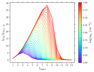
Figure 6: CO SLEDs obtained from LVG modelling, for T_kin = 30 K, using RADEX (van der Tak et al., 2007). The CO line flux normalized to the CO(1-0) line is plotted as a function of the upper rotational quantum number J. Different values in H₂ density are shown by the colour bar.

Importantly, the emitted CO flux is proportional to the source solid angle (e.g., Weiß et al., 2007b). As our observations are not able to constrain the size of the emitting source, we focus on line ratios in this paper. These LVG models will therefore represent only solutions for the component of highly excited gas, which likely coexist with a less excited component emitting the [Ci](2-1) emission that we observe in some of our targets. Indeed, it has been shown that emission from species with very different critical densities likely originate from gas at different densities (e.g., Harrington et al. 2021), and also on different scales (e.g., Emonts et al. 2014; Casey et al. 2018; Spingola et al. 2020).

We first find models that reproduce the observed upper limits on the CO(7-6)/CO(6-5) line ratios. In our dataset there are only three sources for which it was possible to estimate an observed $I_{\rm CO(7-6)}/I_{\rm CO(6-5)}$ upper limit: the quasars with IDs 8, 43 and 50 (see Table 2). For these sources, we selected LVG models constrained by their observed $I_{\rm CO(7-6)}/I_{\rm CO(6-5)}$ ratio and found densities in the range n${}_{\rm H_{2}}\sim$10³-10^4.4cm^-3. These models constrained the peak of the SLED to be at J$\sim$3-7, and the molecular gas masses to be (0.5 - 64.1)$\times$10¹¹M_⊙ when considering the predicted $I_{\rm CO(1-0)}$ from the SLEDs. These results are shown in the fifth column of Table 4.

It is noteworthy that using a higher T_kin in our LVG models, for instance T_kin = 50 K (found in some high-$z$ quasars, e.g., Weiss et al. 2007a; Riechers et al. 2011), implies an upper limit in the molecular masses $\sim$32$\%$ lower, i.e. this difference does not alter our results significantly. In contrast, using a lower T_kin, for example T_kin = 20 K, implies non-physical values for the upper limit in the molecular masses of up to $\sim$10¹³M_⊙.

4.3 Molecular mass constraints from a joint CO and [Ci] analysis

After applying the CO constraint explained above, we set another condition based on the molecular gas masses already estimated from the [Ci](2-1) transition (see Section 4.1). As $\alpha$ is fixed, this condition is identical to impose a constraint on the CO(1-0) luminosity. We caution that this approach may introduce a bias in our calculation, which depends on the goodness of the assumed parameters to model the molecular mass from [Ci], and on $\alpha$ itself with respect to the physical conditions in each individual source. Observations of the CO(1-0) transition for these sources are definitely needed to confirm this methodology.

For each source, this step excluded some of the LVG models at the lowest densities selected in Section 4.2. In this way, we obtained the final CO SLEDs from the union of the CO and [Ci] constraints. We show these final constrained CO SLEDs in Fig. 7 for quasars with IDs 8, 43 and 50. Their ranges of molecular masses using these joint constraints are (0.7-1.5)$\times 10^{11}\rm M_{\odot}$, (0.5-0.9)$\times 10^{11}\rm M_{\odot}$ and (0.5-1.5)$\times 10^{11}\rm M_{\odot}$, respectively. These values are also listed in the second to last column of Table 4.

Fig. 8 shows the CO SLEDs obtained in this work (discontinuous lines) in comparison to three $z\sim$3 quasars with well sampled SLEDs (grey continuous lines), Cloverleaf ($z$ = 2.6, Weiss et al. 2007a; Bradford et al. 2009), MG 0751+2716 ($z$ = 3.2, Weiss et al. 2007a) and PSS1409 ($z$ = 2.6, Weiss et al. 2007a). From this figure, we see that none of the SLEDs obtained in this work are similar in shape to those three obtained previously, indicating that our quasars have different physical properties. Our results yield SLEDs with J peak somewhat lower than the expected range for quasars (J$\sim$6-8), varying from J$\sim$5 to J$\sim$7.

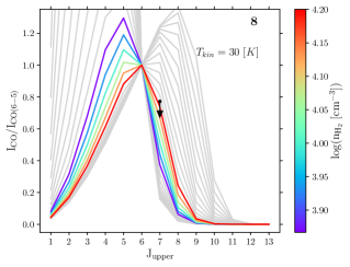
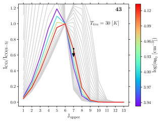
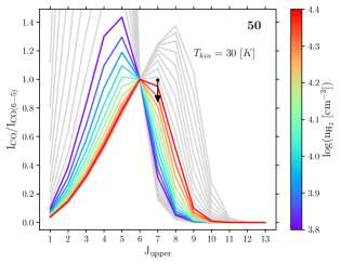
Figure 7: CO SLEDs (at T_kin = 30 K) obtained with the joint CO and [Ci] constraints, for the sources with IDs 8, 43 and 50 (top, middle and bottom panels, respectively), the SLEDS that can fit the joint constraints are represented by the coloured curves. The ladders show the CO line flux normalized to the CO(6-5) line as a function of rotational quantum number J, and the vertical black arrow represents the observed upper limit on the CO(7-6)/CO(6-5) ratio for each source. The different values in H₂ density are shown by the colour bar. The grey curves in the background show the discarded CO SLEDs (from Fig. 6).

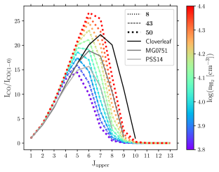
Figure 8: CO SLEDs for the sources with IDs 8, 43 and 50 (discontinuous lines; see legend) compared to the SLEDs for the quasars Cloverleaf, MG0751 and PSS14, obtained by Weiss et al. (2007a) (continuous grey lines). The ladders correspond to the CO line flux normalized to the CO(1-0) line as a function of rotational quantum number J.

The six sources with IDs 3, 7, 13, 18, 29 and 39, have only upper limits for the targeted CO transitions. Our observations are therefore not able to put any constraint on the SLED of these sources. To compute the upper limits for the CO(1-0) luminosity, we assumed that the models selected for the previous three sources with IDs 8, 43 and 50, apply to the full observed sample.

We first selected the CO SLEDs found for the quasars with IDs 8, 43 and 50 (shown in Fig. 8). Depending on which emission line upper limit flux was measured for each of the six sources mentioned above, we used the CO(1-0)/CO(6-5) and/or CO(1-0)/CO(7-6) ratios. Then, we multiplied these CO ratios by the observed upper limit flux for each of them. After this, we estimated upper limits for the molecular gas masses of the six quasars with IDs 3, 7, 13, 18, 29 and 39. For the sources that have flux upper limits for both CO lines (quasars with IDs 13, 29 and 39), two upper limits in molecular gas mass were derived and the higher value was selected.

To summarize: the resulting molecular masses of our sample, obtained from applying only the CO constraints, are in the range of (0.5 - 64.1)$\times$10¹¹M_⊙ for the sources with IDs 8, 43 and 50, and are <6.9$\times$10¹¹M_⊙ for the objects with IDs 3, 7, 13, 18, 29 and 39. We note that the range mentioned includes masses of the order of 10¹²M_⊙, which are implausible given the expected dark-matter halo mass for these quasars ($M_{\rm DM\sim}10^{12.5}$ M_⊙, e.g., White et al. 2012). These values are also much higher than the values found in the literature for other high-$z$ quasars ($\sim$10⁹-10${}^{11}\rm M_{\odot}$, e.g., Weiß et al. 2003; Walter et al. 2011; Anh et al. 2013; Hill et al. 2019). These high masses are caused by models with densities of n${}_{\rm H_{2}}\sim$10³-10^3.8cm^-3. This disagreement with the literature values suggests that such low densities are not plausible in explaining our current constraints on the emission from the high-J CO transitions. We note that the molecular gas masses obtained from applying the CO and [Ci] constraints jointly, remove such models.

We emphasize that the final selected densities (n${}_{\rm H_{2}}\sim$10^3.8-10^4.4cm^-3, see Fig. 8) represent those values needed by the high-J CO lines to match the molecular masses estimated from [Ci](2-1). These densities should not be regarded as representative of those emitting the [Ci](2-1) line, unless this emission is more extended than the high-J CO transitions.

The molecular masses that are finally derived after applying a more restricted set of models are in the range of 0.4 - 6.9$\times$10¹¹M_⊙ for quasars with IDs 3, 8, 29, 39, 43 and 50, and <1.1$\times$10¹¹M_⊙ for quasars with IDs 7, 13 and 18. The brightest of our detected sources still has an estimated molecular gas mass that is higher than typically found in the literature. We will discuss this further in the next sections.

We finally check the molecular gas mass estimate for ID 3 and ID 39, for which we identify [Ci](2-1) based on the uncertain C iv systemic redshift (section 3.1). In the case the detected lines are CO(7-6) instead of [Ci](2-1), the final models shown in Figure 8 would imply molecular gas masses of (1.2 - 4.5)$\times$10¹¹M_⊙ and (0.2 - 0.6)$\times$10¹¹M_⊙, respectively. These values would still confirm our findings, with ID 3 having a large molecular mass.

5 Comparison with the large-scale Ly$\alpha$ emission

To investigate any relation between the molecular gas phase and the cool halo gas, in this section we compare the APEX observations with the Ly$\alpha$ line properties of the associated large-scale nebulae discovered with MUSE (Arrigoni Battaia et al., 2019a). First, we focus on finding any trend in the properties of each phase when compared with the other. Secondly, we study the line emission locations and profiles.

5.1 Molecular lines versus Ly${\rm\alpha}$ line properties

The FWHM of molecular lines from high-redshift galaxies are frequently used as a dynamical mass estimator (assuming a rotating disk geometry, e.g., Walter et al., 2003; Narayanan et al., 2009; Wang et al., 2013), and hence their stellar mass and therefore their halo mass can be determined (see Section 6.1.1 for further discussion). As halos of different masses are expected to be characterised by different fractions of cool and hot gas (e.g., Dekel & Birnboim, 2006), the FWHM of molecular lines could show important trends with the Ly$\alpha$ properties. For instance, more massive halos should in principle show larger FWHM of the molecular lines and smaller fractions of cool gas, with consequently smaller Ly$\alpha$ luminosities (L_Lyα) and Ly$\alpha$ areas compared to less massive halos. We start by comparing the FWHM of the observed molecular lines with the total L_Lyα, the average Ly$\alpha$ surface brightness SB_Lyα, and the area encompassed by the Ly$\alpha$ emission by the nebulae surrounding the quasars in our sample.

Figure 9 shows this comparison for the different sources in our sample (represented by different colours). Specifically, the left panel shows the FWHM of the molecular lines as a function of SB_Lyα (corrected for the cosmological dimming), the central panel shows the FWHM versus L_Lyα, and the right panel shows the FWHM versus the area of the Ly$\alpha$ nebulae. The legend in each panel indicates the different markers used for the different molecular lines (CO(6-5) and [Ci](2-1)).

From this figure, we find that there is no clear correlation between FWHM of the molecular lines and Ly$\alpha$ properties. Also, we note that all the quasars show similar values of FWHM (in the range of 329 - 943 km s^-1, average FWHM 647$\pm$129 km s^-1), considering the uncertainties. In the literature, the molecular linewidths (CO and [Ci] lines) found for high-$z$ quasars have values between $\sim$150 - 450 km s^-1 (e.g., Weiß et al., 2003; Weiß et al., 2007b; Walter et al., 2011; Schumacher et al., 2012; Venemans et al., 2017). The values found for our quasars are larger on average. For example, quasars with IDs 29 and ID 50 have a FWHM of 943$\pm$249 km s^-1 ([Ci](2-1) emission) and 707$\pm$100 km s^-1 (CO(6-5) emission) respectively, suggesting that they have a different kinematics and/or physical properties compared to the quasars studied in the literature.

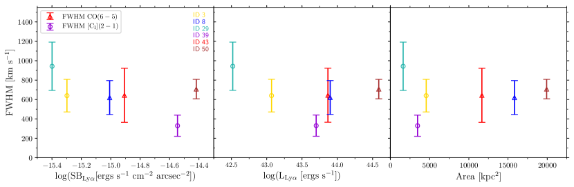
Figure 9: FWHM of the detected CO(6-5) (triangles) and [Ci](2-1) (circles) emission lines versus Ly$\alpha$ surface brightness corrected for cosmological dimming (first panel), the total Ly$\alpha$ luminosity (second panel), and physical area (third panel) for the large-scale Ly$\alpha$ nebulae discovered around the quasars in our sample (Arrigoni Battaia et al., 2019a).

As molecular gas is expected to form from the cooling of 10⁴K gas (e.g., Dalgarno & McCray, 1972), one may naively expect to observe the largest molecular reservoirs in sources with the largest and brightest Ly$\alpha$ nebulae. As a next step, we focus on the molecular gas masses obtained from the joint constraints from CO and [Ci] (see Section 4.3), and compare them to L_Lyα, SB_Lyα and the area of the large-scale nebulae.

The results of this analysis are presented in Figure 10, where the colours represent different sources, the vertical dashed lines are ranges and the arrows upper limits of the estimated molecular gas masses. The horizontal black lines represent the expected molecular mass for the quasar host galaxies on the main sequence (MS) of star-forming galaxies (log($M_{\rm H_{2}}[M_{\odot}]$) = 10.98${}^{+0.32}_{-0.51}$), on 4$\times$MS (log($M_{\rm H_{2}}[M_{\odot}]$) =11.29) and 10$\times$MS (log($M_{\rm H_{2}}[M_{\odot}]$) =11.51). These values were computed under the following assumptions: i) a quasar halo mass of log($M_{\rm halo}[M_{\odot}]$) = 12.68${}^{0.81}_{-0.67}$ (for z$\sim$3 quasars), estimated in the study of Kim & Croft (2008) from Ly$\alpha$ forest statistics (this value encompasses estimates from quasar clustering, e.g., Shen et al. 2007; White et al. 2012; Timlin et al. 2018), ii) the $M_{\rm halo}-M_{*}$ relation from Moster et al. (2018) to estimate the stellar mass of the objects in our sample, and iii) a molecular gas fraction expected for objects on MS, 4$\times$MS and 10$\times$MS of star-forming galaxies, as defined in the empirical relation of Tacconi et al. (2018). The grey shaded region represents the large uncertainties in the calculation for 1$\times$MS. We note that quasars hosts are estimated to have star formation rates higher or similar to MS galaxies at the same redshift (e.g., Zhang et al. 2016; Shangguan et al. 2020; Jarvis et al. 2020; Circosta et al. 2021). The histogram shows the $M_{\rm H_{2}}$ distribution for our sample (red) and for a sample of $z\sim$2.5 - 3 quasars (blue) extracted from the literature as explained in the figure caption. The molecular masses reported for these quasars are overall below the computed predictions (see histogram in Fig. 10), possibly indicating some gas depletion with respect to similarly massive star-forming galaxies.

It is clear that the molecular gas masses of the quasars with APEX detections are in agreement with the expected values for MS galaxies, with the exception of quasars with IDs 3 and 29, which have masses well above the MS. Intriguingly, these two objects characterised by the highest molecular gas masses are associated with the Ly$\alpha$ nebulae with the lowest values of L_Lyα and SB_Lyα. The third panel of Fig. 10 shows that the most massive molecular reservoirs are associated with some of the smallest nebulae. They also have the highest FWHM [Ci](2-1) emission lines (see Fig. 9). We will discuss this result in more detail in Section 6.3.

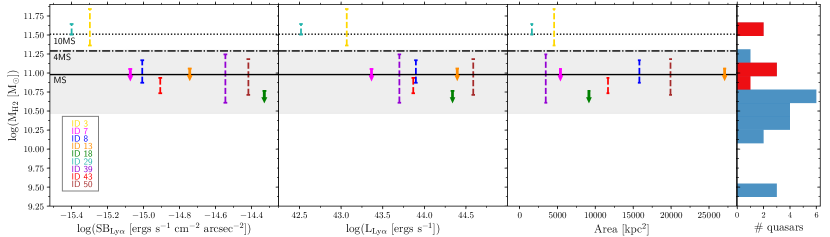
Figure 10: Molecular gas mass $\rm M_{H2}$ derived from the joint CO and [Ci] constraints versus Ly$\alpha$ surface brightness corrected for cosmological dimming (first panel), the total Ly$\alpha$ luminosity (second panel), and physical area (third panel) for the large-scale Ly$\alpha$ nebulae discovered around the quasars in our sample (Arrigoni Battaia et al. 2019a). The ID numbers of the sources are shown in the first panel. The vertical dashed lines represent ranges of $\rm M_{H2}$, and the arrows indicate upper limits (see Table 4). The horizontal lines show the expected location of massive star-forming main sequence MS, 4$\times$MS and 10$\times$MS galaxies using the gas fractions in Tacconi et al. (2018) and the halo mass-stellar mass relation in Moster et al. (2018). The grey area is the uncertainty on this expectation, for 1$\times$MS. The histogram show the $\rm M_{H2}$ distribution for our sample considering the average values of the mass ranges (red), and for a sample of $z\sim$2.5 - 3 quasars (blue) extracted from the literature (Barvainis et al. 2002; Weiß et al. 2003; Beelen et al. 2004; Walter et al. 2011; Schumacher et al. 2012; Hill et al. 2019; Bischetti et al. 2021), whose $\rm M_{H2}$ have been estimated with different molecular gas tracers and have a typical uncertainty of $\sim\ 0.1$ dex.

5.2 Molecular tracers vs Ly$\alpha$ line profiles

Now that we have a more robust estimate of the systemic redshift $z_{\rm mol,sys}$ for some of our sources, we can compare its location with the redshift of the discovered Ly$\alpha$ nebulae, assessing if the Ly$\alpha$ emission spans similar velocity ranges with respect to the molecular phase. For this purpose, we compare the molecular and Ly$\alpha$ line profiles extracted within the same aperture (the APEX beam; see Fig. 2), and also compare those with the quasar spectra.

Figures 11 and 12 show the normalized APEX CO(6-5) and [Ci](2-1) detections (blue) in comparison to their normalized Ly$\alpha$ nebula spectrum (upper row) and quasar spectrum (bottom row). The quasar spectra have been extracted within circular apertures of 1.5 arcsec radius. The vertical red dashed line represents the current systemic redshift estimated from the molecular lines and the grey shaded area corresponds to its uncertainty (see Section 3.2).

From both figures, we note that some of the peaks of the Ly$\alpha$ nebulae present a significative shift from the current systemic redshift. For each object, we listed these velocity shifts $\Delta v_{\rm Ly\alpha Neb-mol}$ between the quasar systemics $z_{\rm mol,sys}$ and the Ly$\alpha$ of the nebulosities in the last column of Table 3. The values of $\Delta v_{\rm Ly\alpha Neb-mol}$ are in the range of -423 to 1236 km s^-1, with the quasars with ID 8 (or UM683) and ID 43 (or CTSH22.05) having the bluest and the reddest shift, respectively. The velocity shifts do not show any trend with respect to the Ly$\alpha$ physical properties explored in this paper. Considering that the Ly$\alpha$ photons experiment changes in frequency due to the scattering processes, these shifts can be an indication of bulk inflows (blueshift) or outflows (redshift) (e.g., Prescott et al., 2015; Dijkstra, 2017).

Figure 13 shows the velocity shifts between $z_{\rm sys}$ and $z_{\rm mol,sys}$ (blue), and redshift of the Ly$\alpha$ nebulae and $z_{\rm mol,sys}$ (orange). The now obtained systemic redshifts from molecular tracers are found to be, in most of the cases, more consistent with the Ly$\alpha$ nebular redshifts, showing an average shift of 176$\pm$39 km s^-1 (red vertical line). We note that this shift is larger than the average shift found at $z\sim 6$, 69$\pm$36 km s^-1 (Farina et al., 2019), obtained by comparing [Cii] redshifts and the nebular redshifts for nine sources (green vertical line). The small number statistics hampers any conclusion from this comparison. For example, if we remove from our sample the radio-loud object, ID 3, we would get a smaller average shift of 46$\pm$35 km s^-1, which is consistent with the work by Farina et al. (2019).

This analysis shows that the systemic redshifts obtained from Civ are not reliable in 4 out of 6 cases ($\sim 70$%). This poor reliability was already indicated by the large velocity shifts of the extended nebular Ly$\alpha$ emission and the Civ redshifts in surveys targeting $z\sim 2-3$ quasars, reporting values as high as $\sim 6000$ km s^-1 (Arrigoni Battaia et al., 2019a; Cai et al., 2019). The same works found that the peak of the nebular emission has smaller velocity shifts with respect to the observed peak of the Ly$\alpha$ emission of the quasar. Figures 11 and 12 indicate that for 3 out of 6 quasars (ID 3, 29, and 50), this was the case because of that peak being at the real systemic. We discuss the most significant shifts between $z_{\rm mol,sys}$ and the redshift of the Ly$\alpha$ nebulae in Section 6.2.

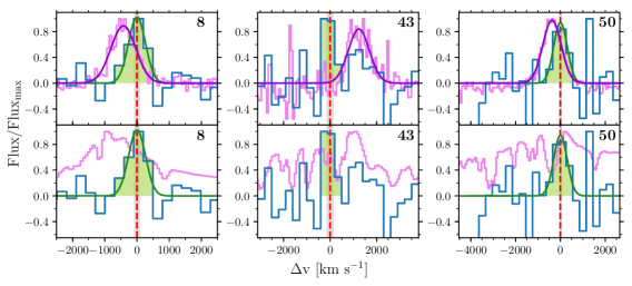
Figure 11: Top panels: Normalized APEX CO(6-5) emission (blue) of the three detected sources, ID 8, ID 43, and ID 50 compared with the nebulae Ly$\alpha$ emission from MUSE (magenta) extracted within the APEX beam (see Figure 2). The APEX spectra are shown with a bin size of 300 km s^-1. Each quasar ID number is shown in the top right corner of each panel. The red vertical lines with grey shaded area correspond to the systemic redshift estimated in this work with its uncertainty. The dark green curves and green shaded areas follow the same notation as in Figure 4. To guide the eye, the purple curves represent a Gaussian fit applied to the Ly$\alpha$ emission lines. Bottom panels: same as above, but comparing with the quasar spectra extracted within a circular aperture of 1.5 arcsec radius.

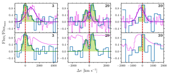
Figure 12: Same as Figure 11, but for the APEX [Ci](2-1) detections (blue).

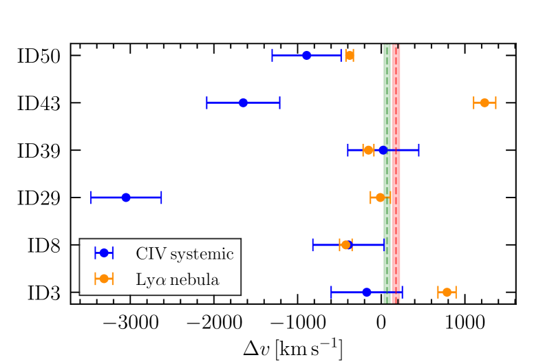
Figure 13: Velocity shifts between $z_{\rm sys}$ (from Civ) and $z_{\rm mol,sys}$ (blue), and redshift of Ly$\alpha$ nebulae and $z_{\rm mol,sys}$ (orange). The green and red vertical dashed lines with errors are the average shift for Ly$\alpha$ nebulae for the sample in Farina et al. (2019) (69$\pm$36 km s^-1; for 9 z$\sim$6 quasars with [Cii] systemic redshifts), and for our work (176$\pm$39 km s^-1), respectively.

6 Discussion

In this section, we discuss different scenarios regarding the quasar host properties found in this work, and we try to interpret the link between the molecular gas content and the large scale Ly$\alpha$ emission. Future studies are essential to confirm or reject what we propose in the following sections.

6.1 Quasar host properties

6.1.1 Dynamical masses

For high-$z$ galaxies, it is possible to derive the dynamical mass of the system using the formula commonly used in the literature (e.g., Walter et al., 2003; Wang et al., 2013; Venemans et al., 2016), assuming rotational support: $M_{\rm dyn}=2.33\times 10^{5}v^{2}_{\rm circ}R[M_{\odot}]$, where $R$ is the disk radius from the observed line and $v_{\rm circ}$ is the maximum circular velocity of the gas disk, which is calculated as $v_{\rm circ}=0.75\times{\rm FWHM}/{\rm sin}(i)$, i.e. it depends on the FWHM of the observed molecular line and inclination $i$ of the galaxy (with respect to the plane of the sky). From our molecular data it is not possible to estimate the parameters $R$ and $i$, for this reason we proceed with a set of assumptions. Arrigoni Battaia et al. in preparation studied the quasar with ID 13 (or PK-1017+109) through ALMA observations, and found a radius of $\sim$3 kpc for this object. This is on the high side of the typical disk radii range found in literature (from molecular gas) for high-z quasar hosts ($\sim$0.5 - 2.5 kpc, e.g.,Carilli et al. 2003; Walter et al. 2004; Aravena et al. 2008; Riechers et al. 2009; Polletta et al. 2011; Schumacher et al. 2012; Molina et al. 2021; Stacey et al. 2021). Here we adopt $R$ = 3 kpc, which is in agreement with our ALMA observations of one of these systems.

Applying the above to five sources in our sample with FWHM estimations, excluding quasar ID 29 that is discussed in Section 6.1.2), we find inclination-dependent dynamical masses in the range of $M_{\rm dyn}{\rm sin}^{2}(i)\sim(0.4-1.9)\times 10^{11}\rm M_{\odot}$ for quasars with IDs 3, 8, 39, 43 and 50. The quasar with ID 39 (or SDSS J0100+2105) is the least massive and the quasar with ID 50 (or SDSS J0819+0823) the most massive. The specific values for these dynamical masses are tabulated in the last colum of Table 4, with uncertainties considering only the errors from their FWHMs. Even though these dynamical masses are highly uncertain, we can get a rough idea on the inclination. Indeed, assuming that the amount of dark matter is negligible on host scales, $M_{\rm dyn}\approx M_{*}+M_{\rm H_{2}}$, where $M_{*}$ is the stellar mass. Assuming that the stellar mass is at least as high as the highest allowed molecular mass from our calculations, we find that two sources, IDs 3 and 39, require relatively small angles ($\sim 20^{\circ}$), while the other four sources, IDs 8, 29, 43 and 50, require an inclination ($\sim 50^{\circ}-60^{\circ}$) close to the mean expected value of ${\rm sin}(i)=0.79$ ($i$ = 57.3^∘, Law et al. 2009).

One caveat is that the estimates are subject to the different molecular lines used. We computed that the CO lines reported in the literature for $z\sim 3$ quasars are on average larger than [Ci] lines by 112$\pm$43 km s^-1 (e.g., Weiß et al. 2003; Schumacher et al. 2012; Banerji et al. 2018; Yang et al. 2019). As these transitions have different critical densities, this could be an indication that the lines trace different gas components, which can be the case if [Ci] and the high-$J$ CO transitions (as CO(6-5)) traces gas also on different scales, with [Ci] extending to outer scales (Schumacher et al., 2012).

6.1.2 The case of Q-0115-30 (ID 29): disk or merger?

In Section 3.1, we showed that the quasar with ID 29 (or Q-0115-30) has a [Ci](2-1) line emission consisting of two Gaussian components separated by $\sim$800 km s^-1. While this line identification needs further confirmation, in this section we discuss their possible origins. This double-peaked feature is unique within our sample and could be produced by a rotating disk or a merger between two molecular gas reservoirs (e.g., Neri et al., 2003; Narayanan et al., 2006; Greve & Sommer-Larsen, 2008; Polletta et al., 2011). In Figure 14 we show this double-peaked line emission at the highest resolution possible (bin size of 80 $\rm km\ s^{-1}$) for which there is still a decent peak S/N of $\sim$2.5 and $\sim$3.5.

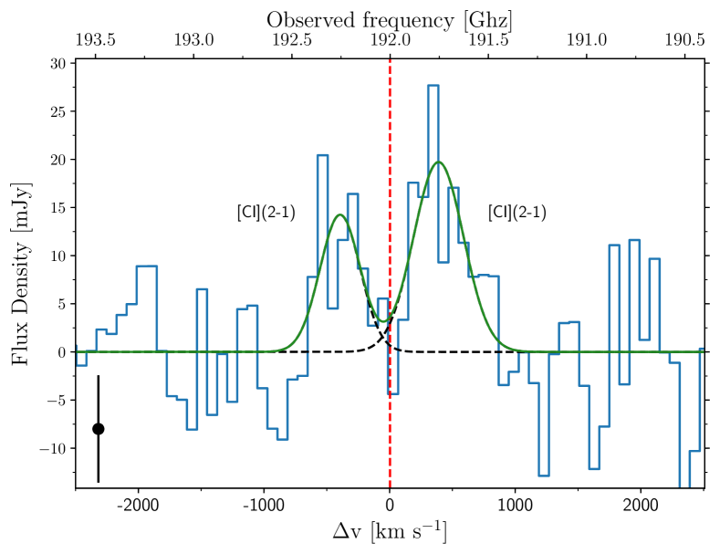
Figure 14: APEX [Ci](2-1) spectral line observation for Q-0115-30 (quasar with ID 29). The spectrum is shown with a bin size of 80 $\rm km\ s^{-1}$, the highest resolution possible. The red vertical line represent the systemic redshift estimated from the molecular lines. The curves and symbol follow the same notation as Figure 5.

We now calculate the dynamical masses, under the assumption that the system is virialized. For the case of the gas distributed in a rotating disk, we estimate the dynamical mass $M_{\rm dyn}^{\rm disk}$ as explained in Section 6.1.1, but considering the velocity difference between the two [Ci](2-1) peaks $\Delta v$, following the formalism of Neri et al. (2003). For the disk radius, we assume a value of $R$ = 3 kpc. We obtain $M_{\rm dyn}^{\rm disk}\ sin^{\rm 2}(i)\sim 4.4\times 10^{11}{\rm M_{\odot}}$. This quasar has the highest dynamical mass of the sample, which is somewhat expected given its larger molecular mass. A larger molecular mass and dynamical mass with respect to the other quasars could also imply a larger dark-matter halo mass.

The combination of an almost edge-on disk and a larger halo mass, could explain a low level of extended Ly$\alpha$ emission as observed for this system. In a unification scenario for AGN (e.g., Urry & Padovani 1995) radiation from the quasar escapes through two ionization cones determined by obscuration from the dust distribution on small scales. Since we observe this object as a quasar, our line-of-sight is inside its ionizing cones. A large fraction of the quasar emission will pass through its massive host molecular disk, and will be absorbed before reaching the CGM. In other words, the obscuration from such a misaligned host galaxy decreases the budget of ionizing photons able to boost the Ly$\alpha$ emission on CGM scales, resulting in a dimmer and less extended Ly$\alpha$ nebula. Any Ly$\alpha$ emission boosted on the scales of the host galaxy likely experience a large number of scatterings and final absorption due to dust, expected to be present in large quantities in such a large molecular reservoir (e.g., Venemans et al. 2017; see Section 6.3 for a rough indication of the dust mass).

On the other hand, a large halo mass implies a smaller fraction of cool gas able to survive the shock-heating process and penetrate the halo down to the host galaxy (e.g., Dekel & Birnboim 2006). In turn, warmer halo and a smaller cool CGM reservoir would result in a lower level of Ly$\alpha$ emission. We therefore conclude that in this scenario, the mass of the halo together with the geometry of the system and Ly$\alpha$ radiative transfer effects could determine the small extent and low SB level of the Ly$\alpha$ nebula surrounding this quasar. Radiative transfer calculations possibly coupled to cosmological hydrodinamical simulations with dust implementations are needed to confirm this interpretation.

For the merger scenario, we can estimate the dynamical mass $M_{\rm dyn}^{\rm merger}$ following Greve & Sommer-Larsen (2008): $M_{\rm dyn}^{\rm merger}=2\times(2.33\times 10^{5}){\rm FWHM}^{2}R[{\rm M_{\odot}}]$, where ${\rm FWHM}$ is the full width half maximum of the observed [Ci](2-1) emission lines, and $R$ is the half projected distance between the two merging objects. We used the same $R$ value assumed in the disk scenario (to obtain a lower limit in $M_{\rm dyn}^{\rm merger}$), and $\rm FWHM=943\pm 249\ kms^{-1}$ (see Table 2), which was calculated as the sum of each single Gaussian fit corresponding to each [Ci](2-1) observed line. We obtain a mass of $M_{\rm dyn}^{\rm merger}=1.2\times 10^{12}{\rm M_{\odot}}$. Assuming that the amount of dark matter is negligible on host scales, the stellar mass is given by $M_{*}\approx M_{\rm dyn}^{\rm merger}-M_{\rm H_{2}}$. Then, using the molecular gas mass range derived from applying the CO and [Ci] constraints, we estimate a total stellar mass in the range $M_{*}=(7.6-8.8)\times 10^{11}{\rm M_{\odot}}$. Following Moster et al. (2018), this stellar mass implies an extremely large dark matter halo mass of $\rm M_{halo}\sim 10^{15.0}-10^{15.1}\ M_{\odot}$.

We also estimated the individual stellar masses of each component of the merging system. The molecular gas masses for the two different objects computed from the atomic carbon masses are $M_{\rm H_{2}}^{\rm obj1}\sim 2.4\times 10^{11}{\rm M_{\odot}}$ and $M_{\rm H_{2}}^{\rm obj2}\sim 3.7\times 10^{11}{\rm M_{\odot}}$, respectively. Then, assuming $M_{\rm H_{2}}^{\rm obj1}/M_{\rm H_{2}}^{\rm obj2}=M_{*}^{\rm obj1}/M_{*}^{\rm obj2}$ , we obtain $M_{*}^{\rm obj1}\sim 2.3\times 10^{11}{\rm M_{\odot}}$ and $M_{*}^{\rm obj2}\sim 3.6\times 10^{11}{\rm M_{\odot}}$. The current MUSE data are not able to verify whether such a massive companion object exists, but this field is characterized by nine faint continuum objects with unknown redshifts within the beam of our APEX observations (Figure 15). These objects do not have any emission lines or absorption features that allow us to verify their redshifts. In particular, we note the presence of one continuum source at $\sim 3\arcsec$ (or $\sim 23$ projected kpc) from the quasar. In summary, given the brightness of the quasar and the seeing-limited MUSE observations, we are not able to assess whether there is an ongoing merger on very small scales. A strongly dust-obscured and massive companion could be missed by our optical observations (e.g., Omont et al. 1996). Finally. we note that within the APEX beam we also find three low-$z$ interlopers (cyan circles in Figure 15), whose redshifts can be clearly determined ($z\sim 0.52,1.05,0.07$). These redshifts ensure that the molecular emission from our targeted object is not contaminated by these sources.

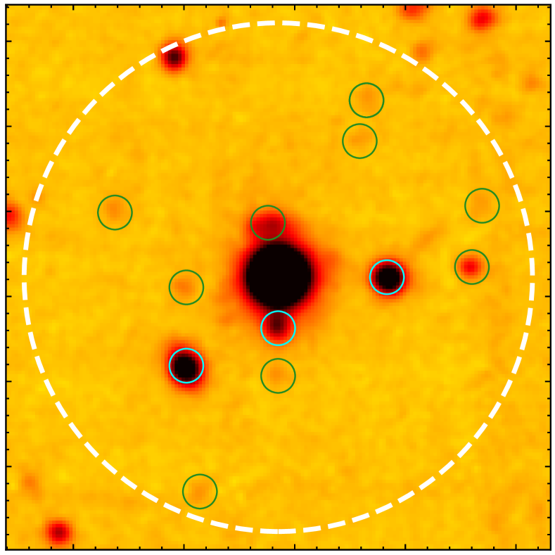
Figure 15: MUSE white-light image for the field around ID 29 (or Q-0115-30, at the center) highlighting the location of continuum sources within the APEX beam for the [Ci](2-1) observations (white dashed circle). Low-$z$ interlopers (cyan circles) and sources with unknown redshift (green circles) are indicated (see Section 6.1.2 for details).

Our consideration of ID 29 shows that its dynamical mass is very large, independent of the origin of the double-peaked [Ci](2-1) line emission. Observing this system with an interferometer (e.g., ALMA, NOEMA) would allow us to map the [Ci](2-1) emission and ascertain whether ID 29 is associated with an exceptionally massive molecular disk or is merging with a similarly massive companion. Such observations, by probing the $\sim 1-2$ mm continuum, would be in turn able to verify the reason why the Ly$\alpha$ nebula around ID 29 is dimmer and less extended than similarly bright quasars.

6.2 Ly$\alpha$ nebulae kinematics with respect to molecular gas

The use of Ly$\alpha$ emission as a tracer of gas kinematics is a complex task due to its resonant nature (e.g., Neufeld 1990). Ly$\alpha$ photons are expected to interact several times with Hydrogen gas before escaping most astrophysical systems (e.g., Dijkstra 2017). During this process, scattered photons can experience both large changes in their frequency and a large displacement in space, possibly washing out any information on gas kinematics. Also, the larger the number of scatterings in a medium, the higher the probability for a Ly$\alpha$ photon to be absorbed by dust. If the dust distribution is not homogeneous, the Ly$\alpha$ line shape could be affected, possibly hiding information on the kinematics of the system.

In Section 5.2 we compared the molecular emission lines observed with APEX, with the Ly$\alpha$ emission obtained with MUSE and integrated within the APEX beam. The main result is that we find velocity shifts between the Ly$\alpha$ emission and the systemic redshift $z_{\rm sys,mol}$ in the range -423 to 1236 km s^-1. The presence of a velocity shift between this Ly$\alpha$ emission line integrated on halos scales and the systemic redshift of the quasar host galaxy, could be associated with a variety of physical processes occurring in the halo, e.g. substructures or gas infalling onto the central quasar, large-scale outflows, rotating structures or projection effects along the line-of-sight (see Arrigoni Battaia et al., 2018a, and references therein). In the following discussion we focus on the possibility that these shifts represent bulk inflows or outflows.

In particular, as indicated by Ly$\alpha$ radiative transfer modelling (e.g, Verhamme et al., 2006; Laursen et al., 2009), photons scattering through outflowing or inflowing gas should appear redshifted or blueshifted, respectively, from the systemic redshift. The quasar with ID 29 has a shift consistent with $z_{\rm sys,mol}$. We cannot therefore draw any firm conclusion for this source with the current dataset. It could be that Ly$\alpha$ radiative transfer effects and a balanced interplay of outflows and inflows result in the absence of a strong line shift or that very fast outflows or inflows bring the gas out of resonance, allowing the observation of Ly$\alpha$ at $z_{\rm mol,sys}$. For the remaining four sources, IDs 3, 8, 39, 43 and 50, we find significant offsets. In particular, IDs 3 and 43 present the largest shifts and also show the largest values of FWHM of the Ly$\alpha$ emission lines in the sample (with ${\rm FWHM_{\rm Ly\alpha}}>1000$ km s^-1), which is typically characterized by relatively quiescent kinematics (median $\rm FWHM_{Ly\alpha}=915\ km\ s^{-1}$). In the following, we review these four sources.

The quasars with IDs 8, 39 and 50 show negative shifts of -423 $\pm$ 76, -152 $\pm$ 64 and -377 $\pm$ 44 km s^-1, respectively, which could indicate an overall inflow signature from CGM scales onto the central quasar. The quasar with ID 39 (or SDSS J0100+2105) is surrounded by one of the less extended Ly$\alpha$ nebulae in our sample (see Fig. 10; Ly$\alpha$ extends out to $\sim 50$ projected kpc). The observed blueshift for this source is lower than the inflow velocities ($v_{\rm in}\approx 0.9v_{\rm vir}\sim 320-460$ km s^-1; Goerdt & Ceverino 2015) expected for the cool gas in quasar host halos ($10^{12}-10^{13}$ M_⊙, e.g., White et al. 2012; Timlin et al. 2018 and references therein). This could be due to projection effects or to the presence of other violent motions (e.g. winds, turbulences) that could wash out the inflow signature.

The observed blueshift for the quasars with ID 8 (or UM683) and ID 50 (or SDSS J0819+0823) is comparable with the inflow velocities expected for the cool gas in quasar host halos. The quasar with ID 8 has an average molecular reservoir and a Ly$\alpha$ nebula with intermediate surface brightness, extending out to $\sim 145$ kpc (Arrigoni Battaia et al. 2019a.) Interestingly, ID 50 is surrounded by one of the brightest and more extended (in area) Ly$\alpha$ nebulae in the QSO museum sample (see Fig. 10; Ly$\alpha$ extends out to $\sim 130$ projected kpc), with a clearly asymmetric morphology. The widths of their integrated Ly$\alpha$ lines, FWHM${{}_{\rm Ly\alpha}=915\pm 46}$ km s^-1 and FWHM${{}_{\rm Ly\alpha}=967\pm 38}$ km s^-1 (for IDs 8 and 50, respectively), may therefore be explained by gravitational motions in such massive halos (${\rm FWHM}_{\rm 1D}^{\rm DM}\sim 580-870$ km s^-1; Arrigoni Battaia et al. 2019a) and by the presence of large turbulence within the cool gas reservoir.

In contrast, the quasars with IDs 3 and 43 show positive shifts of 786$\pm$109 km s^-1 and 1236$\pm$133 km s^-1, respectively, which are suggestive of bulk large-scale outflows. These velocity shifts are overall higher than what has been found in Ly$\alpha$-emitting galaxies (average of $\Delta v\sim$ 200 km s^-1, e.g., Trainor et al. 2015; Prescott et al. 2015; Verhamme et al. 2018), Lyman-break galaxies (average of $\Delta v\sim$ 460 km s^-1, see Dijkstra 2017 and references therein), and are also higher than the values found for other Ly$\alpha$ nebulae, the so called Ly$\alpha$ blobs ($\sim$0 - 230 km s^-1, e.g., Yang et al. 2011; McLinden et al. 2013; Prescott et al. 2015).

The quasar with ID 3 is radio-loud, characterized by a large reservoir of molecular gas and has one of the Ly$\alpha$ nebulae with the lowest surface brightness, extending out to a maximum of $\sim 70$ projected kpc (Arrigoni Battaia et al. 2019a). Its integrated Ly$\alpha$ emission shows the most active kinematics of the sample ($\rm FWHM_{Ly\alpha}=1542\pm 196\ \rm km\ s^{-1}$), which together with the observed large Ly$\alpha$ shift likely indicates that small-scale radio feedback is affecting the surrounding gas distribution in this system. The quasar with ID 43 has an average molecular reservoir and a Ly$\alpha$ nebula with intermediate surface brightness, extending out to $\sim 118$ kpc (Arrigoni Battaia et al. 2019a). Its radio nature is not clear because there are no radio observations of this target in the literature. Its relatively active Ly$\alpha$ kinematics ($\rm FWHM_{Ly\alpha}=1068\pm 142km\ s^{-1}$), together with the large observed positive shift of the Ly$\alpha$ line with respect to CO(6-5) and the asymmetric morphology of the nebula with a northern bright region, might all be hints of outflowing gas in this system.

6.3 Relation between large molecular reservoirs and Ly$\alpha$ nebulae

In section 5.1, we found a tentative trend indicating that the two quasars with the lowest surface brightness for their Ly$\alpha$ nebulae are associated with the highest molecular gas masses. As the molecular gas content is also closely linked to the amount of dust, this could imply that the radiation of these quasars is more obscured by their host galaxies, therefore reducing the reprocessed Ly$\alpha$ emission from the surrounding gas distribution. Two effects could then be in play in the radiative transfer of these systems: first, scattered Ly$\alpha$ photons on small scales (tens of kpc) encounter a very high column density and dusty medium resulting in absorption of the emission, and second, most ionizing photons are not able to escape the massive host galaxy towards the CGM, limiting the detectability of cool halo gas in emission.

On top of this, the halo mass could play an important role in determining the reservoir of cool gas on CGM scales, with more massive halos having a smaller fraction of their gas in this phase. Taking also this aspect into consideration, there are at least two possible interpretations for this tentative trend: 1) IDs 3 and 29 (which present the most massive molecular reservoirs together with dimmer nebulae) occupy similar massive dark matter halos as the rest of quasars in the sample, but their molecular gas fraction (and consequently dust) are higher, resulting in smaller escape of ionizing and Ly$\alpha$ photons, 2) IDs 3 and 29 live in more massive dark matter halos, which are warmer and characterized by a smaller cool gas fraction, hence lower levels of Ly$\alpha$.

Unfortunately, we cannot unambiguously infer the halo masses with the available observations, nor we can firmly quantify obscuration in these systems. Future analysis based on high-resolution interferometric observations and spectra from other CO transitions (e.g., with ALMA, NOEMA) are needed to better constrain the nature of these sources. Such follow-up studies together with constraints on the far-infrared continuum will be able to accurately determine the dust and molecular content of these systems, allowing a better description of the radiative transfer around these quasars.

7 Summary

With the purpose of gaining a new leverage on the gas cycle around $z\sim 3$ quasars, we exploit the frequency window opened-up by SEPIA180 at APEX, targeting the CO(6-5), CO(7-6) and [Ci](2-1) transitions for a sample of 9 $z\sim 3$ quasars already observed with MUSE/VLT. Specifically, these 9 targets (quasars with IDs 3, 8, 13, 18, 29, 39, 43 and 50) cover the most of the parameter space of Ly$\alpha$ nebulae properties in the QSO MUSEUM survey (Arrigoni Battaia et al., 2019a). These data (average rms of 2.6 mJy) allowed us to investigate any relation between the molecular gas content and the large-scale atomic phase ($\sim$10⁴K) as traced by the Ly$\alpha$ emission. The main results of this work are summarized as follows.

• CO(6-5) emission is detected in three sources (quasars with IDs 8, 43 and 50) with fluxes of $3.4\leq\rm I_{CO(6-5)}\leq 5.1$ Jy km s^-1 and $620\leq$ FWHM $\leq 707$ km s^-1, while the [Ci](2-1) emission is detected in other three sources (quasars with IDs 3, 29, and 39) with fluxes of $2.3\leq\rm I_{[C\textsc{i}](2-1)}\leq 15.7$ Jy km s^-1 and $329\leq$ FWHM $\leq 943$ km s^-1.

• The brightest and widest detection in the sample is the [Ci](2-1) line ($\rm I_{[C\textsc{i}](2-1)}\sim$15.7 Jy km s^-1, FWHM$\sim$943 km s^-1) associated to ID 29, which also presents the dimmest and smallest Ly$\alpha$ nebula in the sample.

• We obtained molecular gas masses $M_{\rm H_{2}}$ from the CO and [Ci](2-1) constraints (Sections 4.1 and 4.2). Applying the two estimates together, the molecular masses for sources with detections are in the range $\rm M_{H_{2}}=(0.4-6.9)\times 10^{11}M_{\odot}$, while for quasars with non-detections, the upper limits are $\rm M_{H_{2}}<1.1\times 10^{11}M_{\odot}$. These masses are on the high side of the typical ranges found in the literature ($\sim$10⁹-10¹¹M_⊙) for other $z\sim 3$ quasars, with ID 29 and ID 3 being outliers.

• The systemic redshift of 6 quasars is refined using the CO(6-5) and [Ci](2-1) detections. These new systemic redshifts have an average uncertainty of 74.8 km s^-1.

• We found significant offsets between the extended Ly$\alpha$ nebulae (Ly$\alpha$ emission extracted within the APEX beam) and the newly estimated systemic redshifts in five sources (quasars with IDs 3, 8, 39, 43 and 50). Two of these sources also show the largest values of FWHM_Lyα in our sample ($>$ 1000 km s^-1), which is otherwise characterized by relatively quiescent kinematics (median FWHM_Lyα = 915 km s^-1). In Section 6.2 we discuss how these velocity shifts could be signatures of bulk inflows/outflows. For the quasars with IDs 8, 39 and 50, the nebular Ly$\alpha$ line shows a blueshift of -423 $\pm$ 76, -152 $\pm$ 64 and -377 $\pm$ 44 km s^-1, respectively, which could indicate a large-scale inflow. In contrast, quasars with IDs 3 and 43 have the bulk of the Ly$\alpha$ line redshifted by 786 $\pm$ 109 km s^-1 and 1236 $\pm$ 133 km s^-1, respectively, which can indicate that the bulk of the large-scale gas is outflowing in both cases. For ID 3, this scenario is further strengthened by the fact that this quasar is radio-loud.

• We found that the two most massive molecular reservoirs in our sample (quasars with IDs 3 and 29, $\rm M_{H_{2}}=(2.3-6.9)\times 10^{11}M_{\odot}$ and $\rm M_{H_{2}}=(3.2-4.4)\times 10^{11}M_{\odot}$, respectively) are associated with the dimmest and smallest Ly$\alpha$ nebulae. This suggests that the quasar host galaxy properties are key in understanding the powering and physics of surrounding Ly$\alpha$ nebulae. Obscuration from the host galaxy, due to physical properties (e.g., higher molecular gas fraction, higher dust fraction) or geometry, could reduce the escape of ionizing and Ly$\alpha$ photons emitted by the quasar, ultimately reducing the emission from the cool CGM. This interpretation is further strengthened by the detection of a double-peaked [Ci](2-1) line emission for ID 29, which could be due to an inclined massive molecular disk, likely misaligned with the ionization cones of ID 29 (see Section 6.1.2). Another possibility is that these quasars with more massive molecular reservoirs could be hosted by more massive dark-matter halos. Such halos are expected to be warmer and to show a smaller fraction of cool CGM gas, which in turn would result in lower values of Ly$\alpha$ emission.

These APEX observations therefore suggest that the quasar host-galaxy properties could affect the Ly$\alpha$ radiative transfer, thus regulating the amount of detectable emission on large scales around quasars. Overall, this work stresses the importance of simultaneously studying the physical properties of the multiphase gas reservoirs surrounding quasars. By characterizing the quasar host galaxy properties and system geometry (e.g., systemic redshift, inflow/outflow), future studies will be able to assess the radiative transfer effects affecting the quasar radiation and ultimately better constrain the powering mechanisms for extended gas reservoirs. Deep high-resolution interferometric observations (e.g., with ALMA, NOEMA) are indispensable to map the extent and geometry of the molecular reservoirs, ultimately linking its physics to the other CGM phases.

Data Availability

The data used in this work are available from the ESO Science Archive Facility (https://archive.eso.org/). The fully reduced dataset will be shared upon reasonable request to the corresponding author.

Appendix A Stability of data

We demonstrated the stability of the SEPIA180 receiver by checking if the noise scales down properly when using larger velocity bins. In Figure 16 we show the rms of the final reduced spectra as a function of the bin size, for each of our sources in the different observed tunings. The smallest bin size corresponds to the original resolution of the spectra (i.e., the unbinned data). The solid lines represent the expected variation of the rms ($\rm rms_{\rm expected}$) with respect to the bin size, which was estimated as:

$$\rm rms_{\rm expected}=rms_{\rm original}\ \times\sqrt{binsize_{\rm original}/binsize_{\rm observed}}$$ (6)

where $\rm rms_{\rm original}$ ($\rm binsize_{\rm original}$) is the rms (bin size) at the original resolution, and $\rm binsize_{\rm observed}$ is the bin size used in the final combined spectrum. Each panel has a lower subpanel, which shows the deviation of the observed rms from the predicted value, estimated as $\rm(rms_{\rm observed}\ -rms_{\rm expected})/rms_{\rm expected}$, where $\rm rms_{\rm observed}$ is the final rms obtained in the final binned spectrum.

At a bin size of 300 km s^-1, we obtained a median deviation of only 12$\%$ and 14$\%$ for CO(6-5) and [Ci](2-1), respectively. Such a small deviation ensures that we can preform the analysis discussed in the main text.

Further, as a proof of the stability over time of the calibration of the receiver, in Fig. 17 we show the rms for each scan versus its PWV for the source with ID 39 (J 0100+2105). Each colour indicates a different observation date, spanning several months of APEX operations. These values correspond to both the CO(6-5) and [Ci](2-1) - CO(7-6) observations. A linear fit shown by the grey solid line has been applied to the points, with a resulting squared correlation coefficient of $r^{2}=0.93$ and a residual standard error of $\sigma=0.009$ K. The dashed lines enclose 95 per cent of the measurements (i.e. $\pm$2$\sigma$). Abrupt (vertical) changes of the rms during one observing date (e.g., blue points) indicate strong changes in the airmass of the source. From this figure, we note that data taken under similar PWV and elevation, but in different dates, are characterized by the same rms.

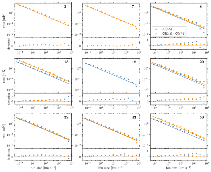
Figure 16: RMS of the final combined spectra as a function of the bin size for each of the nine sources, for CO(6-5) (blue stars) and [Ci](2-1) - CO(7-6) (orange triangles) observations. The ID number of each quasar is shown in the top right corner of each panel. The solid lines represent the expected scaling of the rms with increasing bin size (see section A). The lower subpanels show the deviation of the observed rms with respect to the predicted value, $\rm(rms_{\rm observed}\ -rms_{\rm expected})/rms_{\rm expected}$.

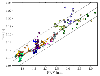
Figure 17: RMS values (for each scan) versus PWV relation for the source SDSS J0100+2105 (ID 39), corresponding to the CO(6-5) and [Ci](2-1) - CO(7-6) observations. Each colour indicates a different observation date. The grey solid line represents a linear fit to the points, and the two dashed lines represent the $\pm$2$\sigma$ ($\pm 0.018$ K) deviation from the fit.

Appendix B Reliability of line detections

We performed two tests to confirm the reliability of the reported lines. First, we performed a negative test that consists in inverting the final combined spectra (multiplying the fluxes by -1) and applying our detection algorithm. Second, we produced jack-knife spectra by inverting each second scan during data reduction. We then apply the detection algorithm to these spectra which should contain only noise.

We stress that in both tests we applied the same detection algorithm used to identify line detections in our spectra (see Section 3). The results of these tests are shown in Table 5. For completeness, we list in footnotes the presence of features that fulfill only partially our selection criteria (i.e. with peak S/N>2).

In summary, we did not find any detections in the negative test. While, in the jack-knife test we found only one line detection (integrated S/N=3.3) for ID8, [Ci](2-1)-CO(7-6) observations. We note that the final [Ci](2-1)-CO(7-6) combined spectrum for this source has a feature at 196.1 GHz (or -328 km s^-1, integrated S/N = 3.1, $I_{\rm line}\sim$3 Jy km s^-1) that according to our jack-knife test, could be a spurious line.

Table 5: Numbers of spurious lines in the negative and jack-knife tests.

		Negative test		Jackknife test
IDa	Quasar	CO(6-5) tuning	[Ci],CO(7-6) tuning	CO(6-5) tuning	[Ci],CO(7-6) tuning
3	J 0525-233	-	0	-	0e
7	SDSS J1209+1138	-	0	-	0f
8	UM683	0	0	0g	1h
13	PKS-1017+109	0	0	0	0i
18	SDSS J1557+1540	0b	-	0	-
29	Q-0115-30	0	0	0	0j
39	SDSS J0100+2105	0c	0	0	0k
43	CTSH22.05	0	0	0	0
50	SDSS J0819+0823	0	0d	0	0

• Identification number taken from the QSO MUSEUM survey (Arrigoni Battaia et al., 2019a).

• The negative spectrum has one feature at $+1200$ km s^-1 with peak S/N>2, but its integrated S/N is only S/N${}_{\rm int}=2.3$.

• The negative spectrum has one feature at $+3500$ km s^-1 with peak S/N>2, but its integrated S/N is only S/N${}_{\rm int}=1.9$.

• The negative spectrum has one feature at $+2000$ km s^-1 with peak S/N>2, but its integrated S/N is only S/N${}_{\rm int}=2.5$.

• This jackknife spectrum has one feature with peak S/N>2, but its integrated S/N is only S/N${}_{\rm int}=2.8$.

• This jackknife spectrum has one feature with peak S/N>2, but its integrated S/N is only S/N${}_{\rm int}=1.9$.

• This jackknife spectrum has one feature with peak S/N>2, but its integrated S/N is only S/N${}_{\rm int}=2.3$.

• This jackknife spectrum has one feature with peak S/N=2.8, and its integrated S/N is S/N${}_{\rm int}=3.3$.

• This jackknife spectrum has one feature with peak S/N>2, but its integrated S/N is only S/N${}_{\rm int}=2.1$.

• This jackknife spectrum has two features with peak S/N>2, but their integrated S/N is only S/N${}_{\rm int}=2.1$ and $2.5$.

• This jackknife spectrum has one feature with peak S/N>2, but its integrated S/N is only S/N${}_{\rm int}=1.9$.

References

- Alaghband-Zadeh et al. (2013) Alaghband-Zadeh S., et al., 2013, MNRAS, 435, 1493
- Anh et al. (2013) Anh P. T., Boone F., Hoai D. T., Nhung P. T., Weiß A., Kneib J. P., Beelen A., Salomé P., 2013, A&A, 552, L12
- Antonucci (1993) Antonucci R., 1993, ARA&A, 31, 473
- Aravena et al. (2008) Aravena M., et al., 2008, A&A, 491, 173
- Arrigoni Battaia et al. (2015) Arrigoni Battaia F., Hennawi J. F., Prochaska J. X., Cantalupo S., 2015, ApJ, 809, 163
- Arrigoni Battaia et al. (2018a) Arrigoni Battaia F., Prochaska J. X., Hennawi J. F., Obreja A., Buck T., Cantalupo S., Dutton A. A., Macciò A. V., 2018a, MNRAS, 473, 3907
- Arrigoni Battaia et al. (2018b) Arrigoni Battaia F., et al., 2018b, A&A, 620, A202
- Arrigoni Battaia et al. (2019a) Arrigoni Battaia F., Hennawi J. F., Prochaska J. X., Oñorbe J., Farina E. P., Cantalupo S., Lusso E., 2019a, MNRAS, 482, 3162
- Arrigoni Battaia et al. (2019b) Arrigoni Battaia F., et al., 2019b, A&A, 631, A18
- Bañados et al. (2018) Bañados E., et al., 2018, Nature, 553, 473
- Bacon et al. (2010) Bacon R., et al., 2010, in McLean I. S., Ramsay S. K., Takami H., eds, Society of Photo-Optical Instrumentation Engineers (SPIE) Conference Series Vol. 7735, Ground-based and Airborne Instrumentation for Astronomy III. p. 773508, doi:10.1117/12.856027
- Banerji et al. (2017) Banerji M., Carilli C. L., Jones G., Wagg J., McMahon R. G., Hewett P. C., Alaghband-Zadeh S., Feruglio C., 2017, MNRAS, 465, 4390
- Banerji et al. (2018) Banerji M., Jones G. C., Wagg J., Carilli C. L., Bisbas T. G., Hewett P. C., 2018, MNRAS, 479, 1154
- Barvainis et al. (2002) Barvainis R., Alloin D., Bremer M., 2002, A&A, 385, 399
- Beelen et al. (2004) Beelen A., et al., 2004, A&A, 423, 441
- Belitsky et al. (2018a) Belitsky V., et al., 2018a, A&A, 611, A98
- Belitsky et al. (2018b) Belitsky V., et al., 2018b, A&A, 612, A23
- Bisbas et al. (2017) Bisbas T. G., van Dishoeck E. F., Papadopoulos P. P., Szűcs L., Bialy S., Zhang Z.-Y., 2017, ApJ, 839, 90
- Bischetti et al. (2021) Bischetti M., et al., 2021, A&A, 645, A33
- Bolatto et al. (2013) Bolatto A. D., Wolfire M., Leroy A. K., 2013, ARA&A, 51, 207
- Boogaard et al. (2020) Boogaard L. A., et al., 2020, ApJ, 902, 109
- Borisova et al. (2016) Borisova E., et al., 2016, ApJ, 831, 39
- Bradford et al. (2009) Bradford C. M., et al., 2009, ApJ, 705, 112
- Bunker et al. (2003) Bunker A., Smith J., Spinrad H., Stern D., Warren S., 2003, Ap&SS, 284, 357
- Cai et al. (2017) Cai Z., et al., 2017, ApJ, 837, 71
- Cai et al. (2019) Cai Z., et al., 2019, ApJS, 245, 23
- Cantalupo et al. (2014) Cantalupo S., Arrigoni-Battaia F., Prochaska J. X., Hennawi J. F., Madau P., 2014, Nature, 506, 63
- Carilli & Walter (2013) Carilli C. L., Walter F., 2013, ARA&A, 51, 105
- Carilli et al. (2003) Carilli C. L., Lewis G. F., Djorgovski S. G., Mahabal A., Cox P., Bertoldi F., Omont A., 2003, Science, 300, 773
- Casey et al. (2018) Casey C. M., et al., 2018, in Murphy E., ed., Astronomical Society of the Pacific Conference Series Vol. 517, Science with a Next Generation Very Large Array. p. 629 (arXiv:1810.08258)
- Circosta et al. (2021) Circosta C., et al., 2021, A&A, 646, A96
- Dalgarno & McCray (1972) Dalgarno A., McCray R. A., 1972, ARA&A, 10, 375
- Decarli et al. (2018) Decarli R., et al., 2018, ApJ, 854, 97
- Decarli et al. (2019) Decarli R., et al., 2019, ApJ, 882, 138
- Decarli et al. (2020) Decarli R., et al., 2020, ApJ, 902, 110
- Decarli et al. (2021) Decarli R., Arrigoni-Battaia F., Hennawi J. F., Walter F., Prochaska J. X., Cantalupo S., 2021, A&A, 645, L3
- Dekel & Birnboim (2006) Dekel A., Birnboim Y., 2006, MNRAS, 368, 2
- Di Matteo et al. (2005) Di Matteo T., Springel V., Hernquist L., 2005, Nature, 433, 604
- Dijkstra (2017) Dijkstra M., 2017, arXiv e-prints, p. arXiv:1704.03416
- Downes & Solomon (1998) Downes D., Solomon P. M., 1998, ApJ, 507, 615
- Elvis (2000) Elvis M., 2000, ApJ, 545, 63
- Emonts et al. (2014) Emonts B. H. C., et al., 2014, MNRAS, 438, 2898
- Emonts et al. (2019) Emonts B. H. C., Cai Z., Prochaska J. X., Li Q., Lehnert M. D., 2019, ApJ, 887, 86
- Farina et al. (2013) Farina E. P., Falomo R., Decarli R., Treves A., Kotilainen J. K., 2013, MNRAS, 429, 1267
- Farina et al. (2014) Farina E. P., Falomo R., Scarpa R., Decarli R., Treves A., Kotilainen J. K., 2014, MNRAS, 441, 886
- Farina et al. (2019) Farina E. P., et al., 2019, ApJ, 887, 196
- Ferrarese & Merritt (2000) Ferrarese L., Merritt D., 2000, ApJ, 539, L9
- Fossati et al. (2021) Fossati M., et al., 2021, MNRAS, 503, 3044
- Fumagalli et al. (2016) Fumagalli M., Cantalupo S., Dekel A., Morris S. L., O’Meara J. M., Prochaska J. X., Theuns T., 2016, MNRAS, 462, 1978
- García-Vergara et al. (2017) García-Vergara C., Hennawi J. F., Barrientos L. F., Rix H.-W., 2017, ApJ, 848, 7
- García-Vergara et al. (2019) García-Vergara C., Hennawi J. F., Barrientos L. F., Arrigoni Battaia F., 2019, ApJ, 886, 79
- Goerdt & Ceverino (2015) Goerdt T., Ceverino D., 2015, MNRAS, 450, 3359
- Goldreich & Kwan (1974) Goldreich P., Kwan J., 1974, ApJ, 189, 441
- Greve & Sommer-Larsen (2008) Greve T. R., Sommer-Larsen J., 2008, A&A, 480, 335
- Gronke & Oh (2018) Gronke M., Oh S. P., 2018, MNRAS, 480, L111
- Gronke & Oh (2020) Gronke M., Oh S. P., 2020, MNRAS, 492, 1970
- Gullberg et al. (2016) Gullberg B., et al., 2016, A&A, 591, A73
- Haiman & Rees (2001) Haiman Z., Rees M. J., 2001, ApJ, 556, 87
- Harrington et al. (2021) Harrington K. C., et al., 2021, ApJ, 908, 95
- Heckman et al. (1991) Heckman T. M., Lehnert M. D., van Breugel W., Miley G. K., 1991, ApJ, 370, 78
- Hennawi & Prochaska (2007) Hennawi J. F., Prochaska J. X., 2007, ApJ, 655, 735
- Hennawi & Prochaska (2013) Hennawi J. F., Prochaska J. X., 2013, ApJ, 766, 58
- Hennawi et al. (2006) Hennawi J. F., et al., 2006, ApJ, 651, 61
- Hennawi et al. (2015) Hennawi J. F., Prochaska J. X., Cantalupo S., Arrigoni-Battaia F., 2015, Science, 348, 779
- Hill et al. (2019) Hill R., et al., 2019, MNRAS, 485, 753
- Hummels et al. (2019) Hummels C. B., et al., 2019, ApJ, 882, 156
- Husband et al. (2015) Husband K., Bremer M. N., Stanway E. R., Lehnert M. D., 2015, MNRAS, 452, 2388
- Husemann et al. (2018) Husemann B., Worseck G., Arrigoni Battaia F., Shanks T., 2018, A&A, 610, L7
- Ikeda et al. (2002) Ikeda M., Oka T., Tatematsu K., Sekimoto Y., Yamamoto S., 2002, ApJS, 139, 467
- Israel & Baas (2002) Israel F. P., Baas F., 2002, A&A, 383, 82
- Ivezić et al. (2002) Ivezić Ž., et al., 2002, AJ, 124, 2364
- Jalan et al. (2019) Jalan P., Chand H., Srianand R., 2019, ApJ, 884, 151
- Jarvis et al. (2020) Jarvis M. E., et al., 2020, MNRAS, 498, 1560
- Kanjilal et al. (2021) Kanjilal V., Dutta A., Sharma P., 2021, MNRAS, 501, 1143
- Kauffmann & Haehnelt (2000) Kauffmann G., Haehnelt M., 2000, MNRAS, 311, 576
- Kereš et al. (2005) Kereš D., Katz N., Weinberg D. H., Davé R., 2005, MNRAS, 363, 2
- Kim & Croft (2008) Kim Y.-R., Croft R. A. C., 2008, MNRAS, 387, 377
- Kormendy & Ho (2013) Kormendy J., Ho L. C., 2013, ARA&A, 51, 511
- Lau et al. (2016) Lau M. W., Prochaska J. X., Hennawi J. F., 2016, ApJS, 226, 25
- Lau et al. (2018) Lau M. W., Prochaska J. X., Hennawi J. F., 2018, ApJ, 857, 126
- Laursen et al. (2009) Laursen P., Razoumov A. O., Sommer-Larsen J., 2009, ApJ, 696, 853
- Law et al. (2009) Law D. R., Steidel C. C., Erb D. K., Larkin J. E., Pettini M., Shapley A. E., Wright S. A., 2009, ApJ, 697, 2057
- Lu et al. (2018) Lu N., et al., 2018, ApJ, 864, 38
- Lyke et al. (2020) Lyke B. W., et al., 2020, ApJS, 250, 8
- Mackenzie et al. (2021) Mackenzie R., et al., 2021, MNRAS, 502, 494
- Matuszewski et al. (2010) Matuszewski M., Chang D., Crabill R. M., Martin D. C., Moore A. M., Morrissey P., Rahman S., 2010, in McLean I. S., Ramsay S. K., Takami H., eds, Society of Photo-Optical Instrumentation Engineers (SPIE) Conference Series Vol. 7735, Ground-based and Airborne Instrumentation for Astronomy III. p. 77350P, doi:10.1117/12.856644
- McLinden et al. (2013) McLinden E. M., Malhotra S., Rhoads J. E., Hibon P., Weijmans A.-M., Tilvi V., 2013, ApJ, 767, 48
- Molina et al. (2021) Molina et al., 2021, arXiv e-prints, p. arXiv:2101.00764
- Morrissey et al. (2012) Morrissey P., et al., 2012, in McLean I. S., Ramsay S. K., Takami H., eds, Society of Photo-Optical Instrumentation Engineers (SPIE) Conference Series Vol. 8446, Ground-based and Airborne Instrumentation for Astronomy IV. p. 844613, doi:10.1117/12.924729
- Moster et al. (2018) Moster B. P., Naab T., White S. D. M., 2018, MNRAS, 477, 1822
- Narayanan et al. (2006) Narayanan D., et al., 2006, ApJ, 642, L107
- Narayanan et al. (2009) Narayanan D., Cox T. J., Hayward C. C., Younger J. D., Hernquist L., 2009, MNRAS, 400, 1919
- Neri et al. (2003) Neri R., et al., 2003, ApJ, 597, L113
- Neufeld (1990) Neufeld D. A., 1990, ApJ, 350, 216
- Novak et al. (2019) Novak M., et al., 2019, ApJ, 881, 63
- O’Sullivan et al. (2020) O’Sullivan D. B., Martin C., Matuszewski M., Hoadley K., Hamden E., Neill J. D., Lin Z., Parihar P., 2020, ApJ, 894, 3
- Omont et al. (1996) Omont A., Petitjean P., Guilloteau S., McMahon R. G., Solomon P. M., Pécontal E., 1996, Nature, 382, 428
- Ouchi et al. (2004) Ouchi M., et al., 2004, ApJ, 611, 685
- Papadopoulos & Greve (2004) Papadopoulos P. P., Greve T. R., 2004, ApJ, 615, L29
- Peeples et al. (2019) Peeples M. S., et al., 2019, ApJ, 873, 129
- Perley et al. (2011) Perley R. A., Chandler C. J., Butler B. J., Wrobel J. M., 2011, ApJ, 739, L1
- Polletta et al. (2011) Polletta M., Nesvadba N. P. H., Neri R., Omont A., Berta S., Bergeron J., 2011, A&A, 533, A20
- Porciani et al. (2004) Porciani C., Magliocchetti M., Norberg P., 2004, MNRAS, 355, 1010
- Prescott et al. (2015) Prescott M. K. M., Martin C. L., Dey A., 2015, ApJ, 799, 62
- Prochaska et al. (2013) Prochaska J. X., Hennawi J. F., Simcoe R. A., 2013, ApJ, 762, L19
- Prochaska et al. (2014) Prochaska J. X., Lau M. W., Hennawi J. F., 2014, ApJ, 796, 140
- Rees (1988) Rees M. J., 1988, MNRAS, 231, 91P
- Richards et al. (2006) Richards G. T., et al., 2006, AJ, 131, 2766
- Richstone et al. (1998) Richstone D., et al., 1998, Nature, 385, A14
- Riechers et al. (2006) Riechers D. A., et al., 2006, ApJ, 650, 604
- Riechers et al. (2009) Riechers D. A., Walter F., Carilli C. L., Lewis G. F., 2009, ApJ, 690, 463
- Riechers et al. (2011) Riechers D. A., et al., 2011, ApJ, 739, L32
- Riechers et al. (2013) Riechers D. A., et al., 2013, Nature, 496, 329
- Salak et al. (2019) Salak D., Nakai N., Seta M., Miyamoto Y., 2019, ApJ, 887, 143
- Schmidt (1963) Schmidt M., 1963, Nature, 197, 1040
- Schumacher et al. (2012) Schumacher H., Martínez-Sansigre A., Lacy M., Rawlings S., Schinnerer E., 2012, MNRAS, 423, 2132
- Shangguan et al. (2020) Shangguan J., Ho L. C., Bauer F. E., Wang R., Treister E., 2020, ApJ, 899, 112
- Shen et al. (2007) Shen Y., et al., 2007, AJ, 133, 2222
- Shen et al. (2016) Shen Y., et al., 2016, ApJ, 831, 7
- Shen et al. (2020) Shen X., Hopkins P. F., Faucher-Giguère C.-A., Alexander D. M., Richards G. T., Ross N. P., Hickox R. C., 2020, MNRAS, 495, 3252
- Silk & Rees (1998) Silk J., Rees M. J., 1998, A&A, 331, L1
- Silva et al. (2015) Silva A., Sajina A., Lonsdale C., Lacy M., 2015, ApJ, 806, L25
- Solomon et al. (1992) Solomon P. M., Downes D., Radford S. J. E., 1992, ApJ, 398, L29
- Spingola et al. (2020) Spingola C., et al., 2020, MNRAS, 495, 2387
- Stacey et al. (2021) Stacey H. R., et al., 2021, MNRAS, 500, 3667
- Steinborn et al. (2015) Steinborn L. K., Dolag K., Hirschmann M., Prieto M. A., Remus R.-S., 2015, MNRAS, 448, 1504
- Tacconi et al. (2018) Tacconi L. J., et al., 2018, ApJ, 853, 179
- Timlin et al. (2018) Timlin J. D., et al., 2018, ApJ, 859, 20
- Trainor et al. (2015) Trainor R. F., Steidel C. C., Strom A. L., Rudie G. C., 2015, ApJ, 809, 89
- Travascio et al. (2020) Travascio A., et al., 2020, A&A, 635, A157
- Tumlinson et al. (2017) Tumlinson J., Peeples M. S., Werk J. K., 2017, ARA&A, 55, 389
- Urry & Padovani (1995) Urry C. M., Padovani P., 1995, PASP, 107, 803
- Valentino et al. (2018) Valentino F., et al., 2018, ApJ, 869, 27
- Venemans et al. (2016) Venemans B. P., Walter F., Zschaechner L., Decarli R., De Rosa G., Findlay J. R., McMahon R. G., Sutherland W. J., 2016, ApJ, 816, 37
- Venemans et al. (2017) Venemans B. P., et al., 2017, ApJ, 845, 154
- Verhamme et al. (2006) Verhamme A., Schaerer D., Maselli A., 2006, A&A, 460, 397
- Verhamme et al. (2018) Verhamme A., et al., 2018, MNRAS, 478, L60
- Walter et al. (2003) Walter F., et al., 2003, Nature, 424, 406
- Walter et al. (2004) Walter F., Carilli C., Bertoldi F., Menten K., Cox P., Lo K. Y., Fan X., Strauss M. A., 2004, ApJ, 615, L17
- Walter et al. (2011) Walter F., Weiß A., Downes D., Decarli R., Henkel C., 2011, ApJ, 730, 18
- Wang et al. (2010) Wang R., et al., 2010, ApJ, 714, 699
- Wang et al. (2013) Wang R., et al., 2013, ApJ, 773, 44
- Wang et al. (2016) Wang R., et al., 2016, ApJ, 830, 53
- Wang et al. (2019) Wang F., Wang R., Fan X., Wu X.-B., Yang J., Neri R., Yue M., 2019, ApJ, 880, 2
- Weiß et al. (2003) Weiß A., Henkel C., Downes D., Walter F., 2003, A&A, 409, L41
- Weiß et al. (2005) Weiß A., Downes D., Henkel C., Walter F., 2005, A&A, 429, L25
- Weiss et al. (2007a) Weiss A., Downes D., Walter F., Henkel C., 2007a, in Baker A. J., Glenn J., Harris A. I., Mangum J. G., Yun M. S., eds, Astronomical Society of the Pacific Conference Series Vol. 375, From Z-Machines to ALMA: (Sub)Millimeter Spectroscopy of Galaxies. p. 25
- Weiß et al. (2007b) Weiß A., Downes D., Neri R., Walter F., Henkel C., Wilner D. J., Wagg J., Wiklind T., 2007b, A&A, 467, 955
- White et al. (1994) White G. J., Ellison B., Claude S., Dent W. R. F., Matheson D. N., 1994, A&A, 284, L23
- White et al. (2012) White M., et al., 2012, MNRAS, 424, 933
- Wootten & Thompson (2009) Wootten A., Thompson A. R., 2009, IEEE Proceedings, 97, 1463
- Yang et al. (2010) Yang B., Stancil P. C., Balakrishnan N., Forrey R. C., 2010, ApJ, 718, 1062
- Yang et al. (2011) Yang Y., Zabludoff A., Jahnke K., Eisenstein D., Davé R., Shectman S. A., Kelson D. D., 2011, ApJ, 735, 87
- Yang et al. (2019) Yang J., et al., 2019, ApJ, 880, 153
- Zhang et al. (2016) Zhang Z., Shi Y., Rieke G. H., Xia X., Wang Y., Sun B., Wan L., 2016, ApJ, 819, L27
- van der Tak et al. (2007) van der Tak F. F. S., Black J. H., Schöier F. L., Jansen D. J., van Dishoeck E. F., 2007, A&A, 468, 627