Search for invisible decays of the Higgs boson produced via vector boson fusion in proton-proton collisions at $\sqrt{s}=13\TeV$

Abstract

A search for invisible decays of the Higgs boson produced via vector boson fusion (VBF) has been performed with 101of proton-proton collisions delivered by the LHC at $\sqrt{s}=13\TeV$ and collected by the CMS detector in 2017 and 2018. The sensitivity to the VBF production mechanism is enhanced by constructing two analysis categories, one based on missing transverse momentum, and a second based on the properties of jets. In addition to control regions with and boson candidate events, a highly populated control region, based on the production of a photon in association with jets, is used to constrain the dominant irreducible background from the invisible decay of a boson produced in association with jets. The results of this search are combined with all previous measurements in the VBF topology, based on data collected in 2012 (at $\sqrt{s}=8\TeV$), 2015, and 2016, corresponding to integrated luminosities of 19.7, 2.3, and 36.3, respectively. The observed (expected) upper limit on the invisible branching fraction of the Higgs boson is found to be 0.$18$ (0.$10$) at the 95% confidence level, assuming the standard model production cross section. The results are also interpreted in the context of Higgs-portal models.

0.1 Introduction

A particle compatible with the standard model (SM) Higgs boson () [PhysRevLett.13.321, Higgs:1964ia, PhysRevLett.13.508, PhysRevLett.13.585, Higgs:1966ev, Kibble:1967sv] was discovered at the CERN LHC in 2012 [Aad:2012tfa, Chatrchyan:2012xdj, Chatrchyan:2013lba]. Since then, extensive studies of this particle have been performed with data taken at $\sqrt{s}=7$, 8, and 13, in particular to understand how it couples to other SM particles.

In the SM, the branching fraction to invisible final states, ${\mathcal{B}(\PH\to\text{inv})}$, is only about 0.1% [Dittmaier:2011ti], from the decay of the Higgs boson via $\PZ\PZ^{*}\to 4\PGn$. Several theories beyond the SM (BSM), however, predict much higher values of ${\mathcal{B}(\PH\to\text{inv})}$ ([Belanger:2001am, Datta:2004jg, Dominici:2009pq, SHROCK1982250], as well as Ref. [Argyropoulos:2021sav] and references therein). In particular, in Higgs portal models, the Higgs boson acts as the mediator between SM particles and dark matter (DM) [Djouadi:2011aa, Baek:2012se, Djouadi:2012zc, Beniwal:2015sdl], strongly enhancing ${\mathcal{B}(\PH\to\text{inv})}$.

Direct searches for $\PH\to\text{inv}$ decays have already been performed by the ATLAS [Aaboud:2019rtt, ATLAS:2021gcn] and CMS [Sirunyan:2018owy, CMS:2021far, CMS:2020ulv] Collaborations using data collected at $\sqrt{s}=7$, 8, and 13, and combining the three main Higgs boson production modes, namely gluon-gluon fusion ($\Pg\Pg\PH$), production of a Higgs boson in association with vector bosons ($\PV\PH$, with $\PV=\PWpm$ or ), and vector boson fusion (VBF). Assuming SM production of the Higgs boson, the best observed (expected) 95% confidence level () upper limits on ${\mathcal{B}(\PH\to\text{inv})}$ are set at 0.19 (0.15) by CMS, using data collected at $\sqrt{s}=7$, 8, and 13, and at 0.26 (0.17) by ATLAS using data collected at 13. In both cases, the data at 13were collected in 2016. Combining the latest CMS constraints on both visible and invisible decays within the $\kappa$ framework [Sirunyan:2018koj], the upper bound on ${\mathcal{B}(\PH\to\text{inv})}$ is 0.22 at the 95% , using only the data set collected at 13in 2016.

Thanks to its large production cross section [deFlorian:2016spz] and distinctive event topology, the VBF production mechanism drives the overall sensitivity in the direct search for invisible decays of the Higgs boson. This paper focuses exclusively on the search for $\PH\to\text{inv}$ in the VBF production mode using the LHC proton-proton ($\Pp\Pp$) collision data set collected during 2017–2018, corresponding to an integrated luminosity of up to 101, and on the combination of this search with analyses performed on previous data sets [Khachatryan:2016whc, Sirunyan:2018owy].

Employing a strategy similar to the one used in the previously published analysis [Sirunyan:2018owy], the invariant mass of the jet pair produced by VBF, $m_{\mathrm{jj}}$, is used as a discriminating variable to separate the signal and the dominant backgrounds arising from vector boson production in association with two jets ($\PV\text{+jets}$). Representative Feynman diagrams for the signal and main background processes are shown in Fig. 1.

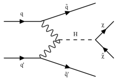
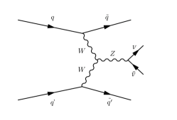
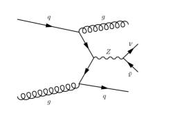
Figure 1: Leading-order Feynman diagrams for the production of the Higgs boson in association with two jets from VBF (left), and representative leading-order Feynman diagrams for the production of a boson in association with two jets either through VBF production (middle) or strong production (right). Diagrams for the production of a boson in association with two jets are similar.

Control regions enriched in $\PV\text{+jets}$ processes are used to constrain the associated background contributions in the signal region. Additional sensitivity is obtained by using $\Pgg\text{+jets}$ events to further constrain the $\PZ(\PGn\PAGn)$ background. In the previous CMS publication, the trigger strategy was based exclusively on the invisible Higgs boson decay products, requiring a high threshold on the missing transverse momentum. With the availability of a trigger based on the jet properties from VBF production, in this analysis, additional sensitivity is achieved by including events with lower missing transverse momentum.

This article is organized as follows. Section 0.2 introduces the CMS detector. Section 0.3 summarizes the data and simulated samples. The event reconstruction is detailed in Section 0.4, followed by the analysis strategy in Section 0.5. Section 0.6 describes the systematic uncertainties. Finally, the results are presented in Section 0.7, with tabulated versions provided in HEPData [hepdata], followed by a summary in Section 0.8.

0.2 The CMS detector

The central feature of the CMS apparatus is a superconducting solenoid of 6m internal diameter, providing a magnetic field of 3.8T. Within the solenoid volume are a silicon pixel and strip tracker, a lead tungstate crystal electromagnetic calorimeter (ECAL), and a brass and scintillator hadron calorimeter, each composed of a barrel and two endcap sections. Hadron forward (HF) steel and quartz fiber calorimeters extend the pseudorapidity $\eta$ coverage provided by the barrel and endcap detectors. Muons are measured in gas-ionization detectors embedded in the steel flux-return yoke outside the solenoid. A more detailed description of the CMS detector, together with a definition of the coordinate system used and the relevant kinematic variables, can be found in Ref. [Chatrchyan:2008zzk].

Events of interest are selected using a two-tiered trigger system [Khachatryan:2016bia]. The first level (L1) is composed of custom hardware processors, which use information from the calorimeters and muon detectors to select events at a rate of about 100kHz [Sirunyan:2020zal]. The second level, known as the high-level trigger (HLT), is a software-based system that runs a version of the full event reconstruction optimized for fast processing, reducing the event rate to about 1kHz.

At the end of 2016, the first part of the CMS detector upgrade program (Phase 1) was undertaken, with the replacement of the inner tracking pixel detector and the L1 trigger system. During the 2016 and 2017 data-taking periods, partial mistiming of signals in the forward region of the ECAL endcaps (${2.5<\abs{\eta}<3.0}$) led to a large reduction in the L1 trigger efficiency [Sirunyan:2020zal]. A separate correction was determined using an unbiased data sample and applied to simulated events to reproduce the loss of efficiency. This problem was resolved before the 2018 data-taking period.

0.3 Data and simulated samples

Data were recorded by several triggers, as detailed in Section 0.5.1, during 2017 and 2018, for maximum integrated luminosities corresponding to 41.5 and 59.8, respectively.

The signal and background processes are simulated using similar Monte Carlo (MC) generator configurations as described in detail in Ref. [Sirunyan:2018owy], and summarized below. Separate independent samples were produced for each data-taking year. The same generator settings were used for the 2017 and 2018 samples.

The Higgs boson signal events, produced through $\Pg\Pg\PH$, VBF, $\PV\PH$, and in association with top quarks ($\PQt{}\PQt{}\PH$), are generated with v2.0 [Nason:2004rx, Frixione:2007vw, Alioli:2010xd, Bagnaschi:2011tu, Nason:2009ai] at next-to-leading order (NLO) approximation in perturbative quantum chromodynamics (pQCD). The signal yields are normalized to the inclusive Higgs boson production cross sections, calculated in Ref. [deFlorian:2016spz] at approximate next-to-NLO (NNLO) in pQCD, with NLO electroweak (EW) corrections. For the VBF production process, an additional event weight is applied to the simulated events to account for EW NLO effects, dependent on the boson transverse momentum (). The correction factor is determined using hawk [Denner:2014cla] and parameterized as $(1-0.000372\pt/\GeVns-0.0304)/0.95$, with the numerator accounting for the full leading order (LO)-to-NLO correction, and the denominator representing the overall normalization effect of the EW correction. The latter is already included in the inclusive cross section, and therefore has to be removed here to avoid double counting.

The $\PZ/\Pgg^{*}(\Pell^{+}\Pell^{-})$+jets, $\PZ(\PGn\PAGn)\text{+jets}$, and $\PW(\Pell\PGn)\text{+jets}$ (with $\Pell=\Pe,\PGm,\PGt$) processes are simulated at NLO in pQCD using v2.6.5 [Alwall:2014hca], with the 5-flavor scheme and the FxFx [Frederix:2012ps] merging scheme, in several bins of boson . Up to two additional partons are included in the final state in the matrix element calculations. These processes are referred to as $\PV\text{+jets}$ (strong) in what follows.

The $\Pgg\text{+jets}$ background is simulated at LO in pQCD using v2.4.2 [Alwall:2014hca], with up to four partons in the final state included in the matrix element calculations [Alwall:2007fs]. We refer to this process as $\Pgg\text{+jets}$ (strong) in the rest of this paper.

The generator is also used for the production of a vector boson, or a photon, in association with two jets exclusively through EW interactions at LO. These are referred to as $\PV\text{+jets}$ (VBF) and $\Pgg\text{+jets}$ (VBF), respectively, in the following.

The LO simulation for the $\Pgg\text{+jets}$ (strong) process is corrected using boson - and $m_{\mathrm{jj}}$-dependent NLO pQCD $K$-factors derived with v2.4.2 [Alwall:2014hca]. The simulations for $\Pgg\text{+jets}$ (strong) and $\PV\text{+jets}$ (strong) processes are also corrected as a function of boson with NLO EW $K$-factors derived in Ref. [Lindert:2017olm]. Similarly, $\PV\text{+jets}$ (VBF) processes are corrected with NLO pQCD $K$-factors derived using the vbfnlo v2.7.0 event generator [Arnold:2008rz, Baglio:2014uba], as functions of boson and $m_{\mathrm{jj}}$. For the $\Pgg\text{+jets}$ (VBF) process, the NLO pQCD corrections, evaluated using , are found to be negligible.

Samples of QCD multijet events are generated at LO using . The and single top quark background samples are produced at NLO in pQCD using v2.0 and v1.0, respectively [Campbell:2014kua, Alioli:2009je, Re:2010bp]. Samples of $\PW\PZ$ and $\PZ\PZ$ events are simulated at LO with v8.205 [Sjostrand:2014zea], while the $\PV\PGg$ and $\PW\PW$ processes are simulated at NLO in pQCD using and  [Melia:2011tj], respectively.

The nnpdf v3.1 [Ball:2014uwa] NNLO parton distribution functions (PDFs) are used for all the matrix element calculations. All generators are interfaced with v8.205 for the parton shower simulation, hadronization, and fragmentation processes. The underlying event description uses the CP5 parameter tune [Sirunyan:2019dfx].

Interactions of the final-state particles with the CMS detector are simulated using  [Agostinelli:2002hh]. Additional $\Pp\Pp$ interactions (pileup) are included in the simulation, and simulated events are weighted to reproduce the pileup distribution observed in data, separately for each data-taking year. The average number of pileup vertices is 32 in the 2017 and 2018 data.

0.4 Event reconstruction

The event reconstruction and object definitions closely follow those of the previous publication [Sirunyan:2018owy]. The main aspects are summarized below.

A global event description is available using the particle-flow (PF) algorithm [Sirunyan:2017ulk]. Using a combination of the information provided by the tracker, calorimeters, and muon systems, the PF algorithm aims to reconstruct individual particles (PF candidates), classifying them as electrons, photons, muons, or charged and neutral hadrons. The final state for this analysis is composed solely of jets from gluons or light-flavored quarks, and missing transverse momentum. We employ explicit vetoes on events containing all other identified types of objects (electrons, photons, muons, hadronically-decaying leptons, heavy-flavored jets), which help to reject background processes with leptonic decays (and bosons), and those containing top quarks.

Electron and photon candidates [CMS:2020uim] are selected in the range $\abs{\eta}<2.5$, while muon [CMS:2018rym] candidates are selected with $\abs{\eta}<2.4$. When considered for event vetoes, candidates are required to satisfy loose identification and isolation criteria. These requirements ensure genuine leptons and photons are discarded with high efficiency. For electrons, the loose working point is referred to as “loose” (“veto” in Ref. [CMS:2020uim]), and has $\simeq$95% efficiency. For photons and muons the loose working point corresponds to efficiencies of $\simeq$90% and $>$99%, respectively. The threshold on loose objects is set to 10for electrons and muons, and 15for photons. When leptons (photons) are explicitly selected to enhance the contributions from $\PV\text{+jets}$ ($\Pgg\text{+jets}$) processes, which is done to populate control regions in data, “tight” identification and isolation criteria are required. These enhance the purity at the price of lower efficiency ($\simeq$70% for electrons and photons, $\simeq$96% for muons). The thresholds are then set to 20for the leading muon, and higher values for the leading electron (40) and photon (230) because of trigger requirements. The subleading electron or muon is required to have $\pt>10\GeV$. In 2018, a section of the hadron calorimeter endcap (HE) was not functional for part of the year, leading to the inability to properly identify electrons and photons in the region $\eta<-1.39$ and azimuthal angle $-1.6<\phi<-0.9$. For data collected during this time, specific electron and photon selection criteria are applied. These are described in more detail in Section 0.5.2.

Jets are reconstructed by clustering all PF candidates associated with the primary interaction vertex using the anti-clustering algorithm [Cacciari:2008gp], with a distance parameter of 0.4, as implemented in the package [Cacciari:2011ma]. The candidate vertex with the largest value of summed physics-object $\pt^{2}$ is taken to be the primary $\Pp\Pp$ interaction vertex. The physics objects used for this determination are the jets, clustered using the jet finding algorithm [Cacciari:2008gp, Cacciari:2011ma] with the tracks assigned to candidate vertices as inputs, and the associated missing transverse momentum, taken as the negative vector sum of the of those jets. Pileup mitigation techniques [Cacciari:2007fd] are used to correct the objects for energy deposits belonging to pileup vertices, as well as to remove objects not associated with the primary interaction vertex. Loose identification criteria are applied on the jet composition to remove contributions from calorimeter noise. To correct the average measured energy of the jets to that of particle-level jets, jet energy corrections are derived using simulated events, as a function of the reconstructed jet and $\eta$. In situ measurements of the momentum balance in dijet, $\Pgg\text{+jet}$, $\PZ\text{+jet}$, and multijet events are used to determine any residual differences between the jet energy scale in data and in simulation, and appropriate corrections are made [Khachatryan:2016kdb]. In simulated events, the jet energy is also smeared to reproduce the jet energy resolution measured in the data [Khachatryan:2016kdb]. For jets with $\pt<50\GeV$, a multivariate discriminant against pileup jets is applied, using a loose working point [Sirunyan:2020foa]. Jets are selected in the range $\abs{\eta}<4.7$ and with $\pt>30\GeV$. Jets with an identified electron, muon, or photon within $\Delta R<0.4$ are rejected, where $\Delta R=\sqrt{\smash[b]{(\Delta\eta)^{2}+(\Delta\phi)^{2}}}$.

The missing transverse momentum vector () is computed as the negative vector sum of all the PF candidates in an event, and its magnitude is denoted as . Any correction applied to individual objects is propagated correspondingly to the  [CMS:2019ctu]. Specific event filters have been designed to reduce the contamination arising from large misreconstructed from noncollision backgrounds [CMS:2019ctu]. For the analysis of the 2018 data, the missing HE section affects the PF reconstruction. The inability to distinguish electrons and photons from jets leads to spurious in the corresponding $\phi$ region as a result of the suboptimal reconstruction of charged and neutral hadrons. Consequently, events with $-1.8<\phi(\ptmiss)<-0.6$ are rejected in data for the part of this data set, around 65% of the total, that is affected. Simulated events in this region are reweighted accordingly to model the efficiency loss.

It has been observed during data taking that the HF detector can, on rare occasions, give rise to unphysical high-energy signals. This occurs in particular when a muon or a charged particle coming from a late showering hadron directly hits one of the photomultiplier tubes that are used to read out the quartz fibers. The photomultiplier tubes are located behind the HF detector, in readout boxes gathering quartz fibers of a given $\phi$ region. The resulting energy is therefore typically spread across several channels of constant $\phi$. Spurious jets can also arise when a high energy muon from machine-induced backgrounds [Bruce:2013tea] undergoes bremsstrahlung in the HF detector. The associated energy deposit is then narrow in both $\eta$ and $\phi$. Although these two effects are uncommon, they lead to large , and a dedicated mitigation technique is therefore applied to reject events with such calorimeter noise. For jets reconstructed in the HF detector, with $\abs{\eta}>2.99$, shower shape variables are constructed based on the associated PF candidates found within $\Delta R<0.4$ of the jet. A central $\eta$ strip size is defined by counting the number of associated PF candidates, $N_{\text{PFCand}}^{\text{cent}}$, with transverse momentum ${\pt>10\GeV}$ within $\Delta\phi<0.05$ of the jet direction. This corresponds to the number of candidates within the same $\phi$ HF tower. The shower widths in both directions are defined as $\sigma_{\eta\eta}$ and $\sigma_{\phi\phi}$, using the pileup-corrected energy-weighted sums of the separations in $\eta$ and $\phi$ between the associated PF candidates with $\pt>3\GeV$ and the jet axis directions.

As stated above, jets stemming from calorimeter noise, called HF noise jets in the following, tend to be either more spread in $\eta$ than in $\phi$, or narrow in both directions. They lead to spurious in the opposite direction in $\phi$. Events are hence rejected if they contain any jet with $\abs{\eta}>2.99$, $\pt>80\GeV$, and $\Delta\phi(\ptvecmiss,\vec{p}_{\mathrm{T}}^{\kern 1.0pt\text{jet}})>2.5$ that does not satisfy the criteria summarized in Table 0.4. The requirements of this selection are chosen to have a mistagging rate smaller than 10% for signal-like jets, while being more than 60–90% efficient at rejecting noise-like jets, depending on their and $\eta$. To correct for mismodelling of these selections in simulation, the selection efficiency on signal-like jets is measured in both data and simulated $\PZ(\Pell\Pell)\text{+jet}$ and $\Pgg\text{+jet}$ events, and scale factors are applied to correct the simulation. The scale factors are measured as functions of jet and $\eta$, and are consistent with unity to within 10%.

Selection applied in the 2017 and 2018 data sets to remove HF jets stemming from calorimeter noise. l c c Observable & $2.99<\abs{\eta_{\text{jet}}}<4.00$ $4.00<\abs{\eta_{\text{jet}}}<5.00$
$\sigma_{\eta\eta}-\sigma_{\phi\phi}$ $<$0.02
$\sigma_{\eta\eta}$ $>$0.02 $<$0.10
$\sigma_{\phi\phi}$ $>$0.02
$N_{\text{PFCand}}^{\text{cent}}$ $<$3

Hadronically-decaying leptons () are identified from reconstructed jets through the multivariate DeepTau algorithm [CMS-DP-2019-033], using a working point that has an average efficiency above 96% for a jet misidentification rate of less than 10%. The candidates are reconstructed with $\pt>20\GeV$ and $\abs{\eta}<2.3$. Jets with an identified loose electron or muon within $\Delta R<0.4$ are rejected before applying the DeepTau algorithm.

The specific features of heavy-flavored jets, in particular the presence of displaced vertices, are used in a multivariate jet tagging method. The “medium” working point of the DeepCSV algorithm from Ref. [Sirunyan:2017ezt] is used to tag quark jets with ${\pt>20\GeV}$ and ${\abs{\eta}<2.4}$ with 68% efficiency, and 1.1 (12)% probability of misidentifying a light-flavor or gluon ( quark) jet as a bottom quark jet.

0.5 Analysis strategy

The distinctive feature of VBF production is a pair of jets originating from light-flavor quarks, with a large separation in $\eta$ ($\Delta\eta_{\mathrm{jj}}$) and therefore a large $m_{\mathrm{jj}}$. The signal region (SR) in this analysis uses selection requirements on the jet pair together with the presence of a significant amount of .

The shape of the $m_{\mathrm{jj}}$ distribution is used to disentangle jet pairs produced in VBF production from other SM processes. When fitting the shape of this distribution, the strong production of the $\PV\text{+jets}$ processes together with the $\Pg\Pg\PH$ signal dominate at low $m_{\mathrm{jj}}$, whereas the VBF-produced $\PV\text{+jets}$ processes populate the high-$m_{\mathrm{jj}}$ tail, together with the VBF signal. The shapes of $m_{\mathrm{jj}}$, $\abs{\Delta\eta_{\mathrm{jj}}}$, and the dijet separation in azimuthal angle ($\abs{\Delta\phi_{\mathrm{jj}}}$) predicted by the simulation are compared between strong and VBF production of both $\PV\text{+jets}$ and signal processes in Fig. 2.

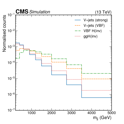
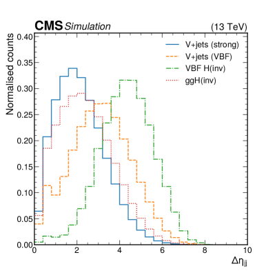
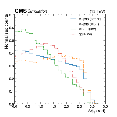
Figure 2: Comparison of shapes of quantities related to the dijet pair. Shown are $m_{\mathrm{jj}}$ (upper), $\Delta\eta_{\mathrm{jj}}$ (lower left), and $\Delta\phi_{\mathrm{jj}}$ (lower right), as predicted by simulation, separating strong and VBF production for $\PV\text{+jets}$ and signal processes.

Whereas similarities are seen between the VBF production of vector bosons and Higgs bosons, there are some differences. First, the respective bosons have different coupling structures, identified as the main reason for the different behaviour in the $\Delta\phi_{\mathrm{jj}}$ distribution [Hankele:2006ma]. Second, the $\PV\text{+jets}$ (VBF) samples include additional diagrams compared with the VBF production, in which the vector boson is produced through a coupling to quarks, and jets are produced from additional EW vertices. For the VBF production, such diagrams are strongly suppressed through the Yukawa mechanism, also leading to differences in the kinematic behaviour.

The dominant $\PV\text{+jets}$ backgrounds are measured using control regions (, , and CRs), in which one or more charged leptons (electrons and muons), or a photon, are required, but the selection on the jets and is kept identical to that in the SR. The MC simulation is used to define transfer factors. These make it possible to predict the $\PV\text{+jets}$ yields in the SR from both the yields measured and predicted in the CRs. The full procedure is described in Section 0.7.

The CR suffers from a lack of statistical precision, particularly in the high-$m_{\mathrm{jj}}$ region, due to the low branching fraction of the boson to a pair of leptons. Because of their similarities, the ratios of the yields of or to production in the SR are constrained, within theoretical uncertainties, to those predicted by the simulation.

In the following subsections, the SR selection is first presented. Then, the data-driven methods used to estimate the $\PV\text{+jets}$ and QCD multijet backgrounds are described. The remaining small contributions expected from diboson and top quark processes are estimated using simulation.

0.5.1 Signal region selection

Two complementary trigger strategies were used to select events online. The first category only uses the information at L1 and in the HLT, and is referred to as the “missing momentum triggered region” (MTR) category in the following. During 2017 and 2018, the HF region was included in the definition of $p_{\mathrm{T,L1}}^{\text{miss}}$, leading to an increase in trigger acceptance when the VBF jets are reconstructed with $3\leq\abs{\eta}\leq 5$, compared with 2016. The $p_{\mathrm{T,L1}}^{\text{miss}}$ thresholds varied between 65 and 90, with a $p_{\mathrm{T,HLT}}^{\text{miss}}$ threshold of 120. After correcting for the L1 mistiming inefficiency described in Section 0.2, this trigger is more than 90% efficient for $\ptmiss>250\GeV$. Loose muon candidates are ignored at L1 and in the HLT when calculating the $p_{\mathrm{T,L1}}^{\text{miss}}$ and $p_{\mathrm{T,HLT}}^{\text{miss}}$ variables, ensuring that the same trigger can be used in the muon CRs. The data collected by these triggers in 2017 and 2018 correspond to integrated luminosities of 41.5 and 59.8, respectively.

The second category uses a combination of and jet information, and is referred to as the “VBF jets triggered region” (VTR) category in the following. After the upgrade of the L1 trigger system [Tapper:2013yva] it was possible to develop an algorithm targeting jets originating from VBF production. This trigger was added after the start of data taking in 2017, and collected a data set corresponding to an integrated luminosity of 36.7during that year. The L1 VBF algorithm requires the presence of at least two jets passing $p_{\mathrm{T}}^{\mathrm{L1}}$ thresholds of 115 (110)for the leading jet and 40 (35)for the subleading jet in 2017 (2018). Pairs are formed from the selected jets, and the pair with the highest invariant mass $m_{\mathrm{jj}}^{\mathrm{L1}}$ must satisfy $m_{\mathrm{jj}}^{\mathrm{L1}}>620\GeV$. The pair is allowed to be formed by two jets with $p_{\mathrm{T}}^{\mathrm{L1}}>40\,(35)\GeV$ if there is a third jet passing the leading-$p_{\mathrm{T}}^{\mathrm{L1}}$ threshold requirement, in 2017 (2018). A corresponding HLT algorithm was designed specifically for the $\PH\to\text{inv}$ analysis, adding a requirement on $p_{\mathrm{T,HLT}}^{\text{miss}}$ with a minimum threshold of 110. At the analysis level, after correcting for the L1 mistiming inefficiency, this trigger is more than 85% efficient for $\ptmiss>160\GeV$ and the leading-$m_{\mathrm{jj}}$ jet pair passing the following requirements: $m_{\mathrm{jj}}>900\GeV$, with thresholds on the two jets forming the leading-$m_{\mathrm{jj}}$ pair of $p_{\mathrm{T}}^{\mathrm{1,2}}>140,70\GeV$. The trigger efficiencies for the two trigger algorithms are available in Appendix LABEL:app:suppMat. Again, loose muon candidates are ignored when calculating the variables at all stages.

We ensure the MTR and VTR categories are orthogonal by requiring $160<\ptmiss\leq 250\GeV$ in the VTR category, and $>250\GeV$ in the MTR category.

To enhance the selection of jets with VBF properties at the analysis level, and to reduce the contamination arising from jet pairs in QCD multijet events, the two leading-jets (or the jets forming the highest-$m_{\mathrm{jj}}$ pair in the VTR category) are required to be in opposite hemispheres of the detector ($\eta_{\mathrm{j1}}\eta_{\mathrm{j}2}<0$). The two selected jets are also required to have $\abs{\Delta\eta_{\mathrm{jj}}}>1$ and $\abs{\Delta\phi_{\mathrm{jj}}}<1.5$ ($\abs{\Delta\phi_{\mathrm{jj}}}<1.8$ in the VTR category). In the MTR category, the $m_{\mathrm{jj}}$ threshold is set to 200to use the full shape of the spectrum to better separate the signal from the background formed by strong $\PV\text{+jets}$ production.

In QCD multijet events, large may arise from mismeasurements of the jet momenta, in which case some jets in the event could be aligned in $\phi$ with the . To reduce the contamination from such events, the minimum value of the azimuthal angle between the vector and any of the first four leading jets ($\pt>30\GeV$), $\min(\Delta\phi(\ptvecmiss,\vec{p}_{\mathrm{T}}^{\kern 1.0pt\text{jet}}))$, is required to be above 0.5 (1.8) in the MTR (VTR) category. Events with possible mismeasurements due to calorimeter noise, which would lead to jets with anomalously large (small) energy fractions coming from neutral (charged) particles, are rejected. This is done by rejecting the event if either of the selected VBF jets has $\abs{\eta}<2.5$ and a neutral (charged) hadron energy fraction $\text{NHEF}>0.8$ ($\text{CHEF}<0.1$). This selection rejects at most 2% of events, independent of the process and uniformly in $m_{\mathrm{jj}}$. A criterion is also applied on the difference between the measured using the PF algorithm and that using only the calorimeters. This difference is required to be less than 50% of the . This selection rejects at most 2 (1)% of all events, mostly at low $m_{\mathrm{jj}}$, for the 2017 (2018) data-taking conditions.

A second source of QCD multijet background is due to the remaining impact of jets originating from HF noise, where the is balanced in $\phi$ with such a jet, and the jet still passes the selection criteria from Table 0.4. Combined with genuine jets from QCD multijet production, such events can pass the SR selection. These large energy deposits are generally close to the outer HF boundary ($\abs{\eta}<3.25$), where the readout boxes are located, though can extend up to $\abs{\eta}=5$.

Finally, a veto on all other types of loosely identified objects (electrons, muons, photons, candidates, and -tagged jets), as described in Section 0.4, is applied.

The criteria for the SR selections are summarized in Table 0.5.1, for the MTR and VTR categories.

Summary of the kinematic selections used to define the SR for both the MTR and the VTR categories. l c c Observable MTR VTR
Choice of pair leading-jets leading-$m_{\mathrm{jj}}$ jets
Leading (subleading) jet $\pt>80\,(40)\GeV$, $\abs{\eta}<4.7$ $\pt>140\,(70)\GeV$, $\abs{\eta}<4.7$
$>$250 $160<\ptmiss<250\GeV$
$\min(\Delta\phi(\ptvecmiss,\vec{p}_{\mathrm{T}}^{\kern 1.0pt\text{jet}}))$ $>$0.5 $>$1.8
$\abs{\Delta\phi_{\mathrm{jj}}}$ $<$1.5 $<$1.8
$m_{\mathrm{jj}}$ $>$200 $>$900
$\abs{\ptmiss-\text{calo }\ptmiss}/\ptmiss$ $<$0.5
Leading/subleading jets $\abs{\eta}<2.5$ $\text{NHEF}<0.8$, $\text{CHEF}>0.1$
HF noise jet candidates 0 (using the requirements from Table 0.4)
candidates $\text{N}_{\tauh}=0$ with $\pt>20\GeV$, $\abs{\eta}<2.3$
 quark jet $\text{N}_{\text{jet}}=0$ with $\pt>20\GeV$, DeepCSV Medium
$\eta_{\mathrm{j1}}\eta_{\mathrm{j2}}$ $<$0
$\abs{\Delta\eta_{\mathrm{jj}}}$ $>$1

Electrons (muons) $\text{N}_{\Pe,\Pgm}=0$ with $\pt>10\GeV$, $\abs{\eta}<2.5\,(2.4)$
Photons $\text{N}_{\Pgg}=0$ with $\pt>15\GeV$, $\abs{\eta}<2.5$
After these selections, the dominant backgrounds come from the $\PV\text{+jets}$ processes. Due to the large branching fraction of the boson decay to neutrinos, the $\PZ(\PGn\PAGn)\text{+jets}$ process accounts for about two-thirds of the total background. After the lepton vetoes and the requirement, the contributions from other decay modes are negligible. The next largest background arises from $\PW(\Pell\PGn)\text{+jets}$ production in which the charged lepton from the boson decay is outside of the acceptance of the tracking detector, leading to additional . In the case of muons, which deposit very little energy in the calorimeters, the is significant. The hadronic decay modes of the boson are rejected by the large requirement. The VBF production of $\PV\text{+jets}$ contributes about 2% of the total $\PV\text{+jets}$ background for $m_{\mathrm{jj}}$ around 200. This increases to about 11% at $m_{\mathrm{jj}}\approx 1.5\TeV$, and to more than 48% for $m_{\mathrm{jj}}>3.5\TeV$.

0.5.2 Lepton-based control regions

As the boson recoil properties are driven by the production mode and are independent of the boson decay mode, the dominant $\PZ(\PGn\PAGn)\text{+jets}$ background is modelled using CRs with leptonic decays of the boson ($\PZ(\Pe\Pe)$ and $\PZ(\PGm\PGm)$). To reduce the contribution from Drell–Yan $\Pgg^{*}$ decays to leptons, the invariant mass of the selected leptons is required to lie in the range 60–120. The lepton selection is chosen to maximize the event yield while still ensuring leptonic boson decays are selected with high purity.

To stay as close as possible to the SR selection, the same trigger as in the SR is used for the $\PZ(\PGm\PGm)$ CR. As a result, systematic uncertainties in the trigger efficiencies largely cancel when estimating the corresponding transfer factors. Instead of the muon veto, a pair of oppositely charged muons, consisting of a tight muon with $\pt>20\GeV$ and a loose muon with $\pt>10\GeV$, is required. All other criteria from Table 0.5.1 are applied. The variable is recalculated ignoring the muons, to mimic the boson recoil.

For the $\PZ(\Pe\Pe)$ CR the triggers used in the SR are inefficient, as electrons deposit their energy in the calorimeter. Single-electron triggers are therefore used. The lowest-threshold trigger requires a minimum of 35and imposes isolation requirements. It is supplemented by an electron trigger with a threshold of 115, but no isolation requirements, as well as by a photon trigger requiring $\pt>200\GeV$. For the last, no isolation criteria are applied, and it does not rely on track reconstruction. Taken together, this set of triggers optimizes the efficiency over the full range. Instead of the electron veto, a pair of oppositely charged electrons, consisting of a tight electron with $\pt>40\GeV$ and a loose electron with $\pt>10\GeV$, is required. The variable is recalculated ignoring the electrons, to mimic the boson recoil.

For the $\PW(\Pell\PGn)\text{+jets}$ background, single-lepton CRs are used. It should be noted that in this case, the $\PW(\Pe\PGn)$ and $\PW(\PGm\PGn)$ CRs favour boson decays with a high-central lepton ($\abs{\eta}<2.5$ (electrons) or 2.4 (muons)), whereas the background expected in the SR consists of boson decays in which the leptons (including leptons) are outside of the acceptance. This has an impact on the distribution. As explained in greater detail in Section 0.7, the impact of the lepton acceptance is accounted for in the definition of the transfer factors between the CRs and the SR, using the simulation. For the $\PW(\Pe\PGn)$ and $\PW(\PGm\PGn)$ CRs, the lepton veto is replaced by the selection of a tight electron (muon) with $\pt>40$ (20), and a veto on any other identified loose electron or loose muon. To reduce the contribution from misidentified electrons stemming from QCD multijet production, the associated with the $\PW(\Pe\PGn)$ decay (not ignoring the electron contribution) is required to be above 80. In the 2018 analysis, due to the missing HE sector in the data, jets in the corresponding $\eta$-$\phi$ area are often identified as electrons or photons, and hence events with an electron in this region are rejected.

0.5.3 The $\Pgg\text{+jets}$ control region

To further constrain the $\PZ(\PGn\PAGn)$ background in the SR, a photon CR is used. At large , the kinematic properties of photon production become similar to those of the $\PZ(\PGn\PAGn)$ process [Lindert:2017olm], and can therefore be used to estimate the latter. Events are selected using a trigger requiring an online photon of at least 200. In the offline analysis, photons are required to be located in the central part of the detector ($\abs{\eta}<1.4442$), have $\pt>230\GeV$ to ensure full trigger efficiency, and pass additional identification criteria based on the properties of the associated energy deposit (supercluster) in the ECAL, as well as the isolation of the photon relative to nearby objects. Exactly one such photon is required, and all other criteria from Table 0.5.1 are applied. The variable is recalculated ignoring the photon, to mimic the boson recoil.

In addition to the desired $\Pgg\text{+jets}$ events with a genuine well-identified and isolated (“prompt”) photon, small contributions from QCD multijet events with hadronic jets misidentified as photons are present in this region (“nonprompt”). To estimate this background contribution, a purity measurement is performed. The measurement is based on the distribution of the lateral width, $\sigma_{i\eta i\eta}$ [CMS:2020uim], of the ECAL supercluster associated with the photon. For prompt photons, the distribution of $\sigma_{i\eta i\eta}$ peaks sharply around values of 0.01 and below, while nonprompt photons show a much smaller peak and a shoulder towards values larger than 0.01. To extract the contamination, a template fit to the $\sigma_{i\eta i\eta}$ distribution is performed in data collected with a looser version of the CR selection. In this looser region, instead of the usual selection that is applied to the VBF jets, we require the presence of a single jet with $\pt>100\GeV$ to enhance the available number of events. Additionally, the photon identification criteria are modified by removing a requirement on $\sigma_{i\eta i\eta}$ that is otherwise included. A template for prompt photons is obtained from simulated $\Pgg\text{+jets}$ events, while a nonprompt template is derived from a data sample that is enriched in nonprompt events by inverting the isolation requirements that are part of the photon identification criteria. The nonprompt fraction is defined as the fraction of nonprompt photons present below the $\sigma_{i\eta i\eta}$ threshold set by the identification criteria. The template fit is performed separately in bins of the photon and yields a nonprompt fraction between around 4% at $\pt=200\GeV$ and 2–3% at $\pt=800\GeV$, depending on the data-taking period. The final QCD multijet contribution is then determined by weighting the events observed in the data by the nonprompt fraction. A 25% uncertainty is assigned to the normalization of the QCD multijet background to account for any mismodelling of $\sigma_{i\eta i\eta}$ in the simulation. The uncertainty is estimated by repeating the measurement while varying the binning of the $\sigma_{i\eta i\eta}$ distribution used for fitting, capturing the effect of the mismodelling. The statistical uncertainty in the determination of the differential $m_{\mathrm{jj}}$ shape is negligible.

0.5.4 Multijet background

The QCD multijet background is estimated using events in data in which the arises from mismeasured jets. Depending on the source of the mismeasurement, the jet that was mismeasured is either balanced in the case of additional HF noise, or aligned with the in $\phi$.

For the multijet background stemming from HF noise, an $m_{\mathrm{jj}}$ template is extracted by inverting the requirements on the HF jet shape variables, hence requiring at least one jet in the event to fail the selection criteria given in Table 0.4. The probability for an HF noise jet candidate to pass or fail the criteria is parameterized as a function of the jet and $\eta$, using events selected to have large and to contain only one HF jet balanced in $\phi$ with the . An event-by-event weight is applied to estimate the contribution in the SR from the “failing” events. The estimated contamination from other SM processes is then removed bin-by-bin for the distribution under study. A closure test is performed by selecting events with the leading-jet within $3<\abs{\eta}<3.25$. With this selection, the signal contamination is $<$2% assuming ${\mathcal{B}(\PH\to\text{inv})}=0.19$, as previously excluded in Ref. [Sirunyan:2018owy]. For events with spurious from noise, one expects a full decorrelation between the measured from the tracker acceptance only, $p_{\mathrm{T,trk}}^{\text{miss}}$, and from the full event, whereas for events with true a correlation exists. Noise events are therefore expected to dominate in the region with large $\Delta\phi$($p_{\mathrm{T,trk}}^{\text{miss}}$,). Data are compared with the estimated template for the $\Delta\phi$($p_{\mathrm{T,trk}}^{\text{miss}}$,) distribution in Fig. 3. From the agreement observed in the closure test in both years, a 20% systematic uncertainty is assigned to the template shape in the SR.

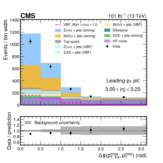
Figure 3: The $\Delta\phi$($p_{\mathrm{T,trk}}^{\text{miss}}$, ) distribution in the SR with the additional requirement that the leading-jet passes $3<\abs{\eta}<3.25$. The 2017 and 2018 data are compared with the sum of the HF noise template and other backgrounds from simulation. The uncertainty band includes only statistical uncertainties in the simulation.

For the second category of multijet events, the requirement on $\min(\Delta\phi(\ptvecmiss,\vec{p}_{\mathrm{T}}^{\kern 1.0pt\text{jet}}))$ is inverted to define a control region enriched in QCD multijet events (QCD CR). The $m_{\mathrm{jj}}$ shape for the contribution of this background in the SR is derived from the yields in data in each $m_{\mathrm{jj}}$ bin in the QCD CR, after subtracting the contributions from $\PV\text{+jets}$, diboson, and top quark processes estimated from simulation, as well as HF noise contributions estimated in the data. The template is normalized as follows. The distribution of $\min(\Delta\phi(\ptvecmiss,\vec{p}_{\mathrm{T}}^{\kern 1.0pt\text{jet}}))$ in data is fit with the sum of templates derived from the simulated $\PV\text{+jets}$, diboson, and top quark events, an HF noise template derived in data; and a functional form $f_{\text{QCD}}$ representing the QCD multijet contribution. The functional form is

$$f_{\text{QCD}}(x)=p_{0}\re^{-p_{1}x}$$ (1)

for the MTR region, and

$$f_{\text{QCD}}(x)=p_{0}\re^{-\frac{(x-p_{1})^{2}}{2p_{2}^{2}}}$$ (2)

for the VTR region. The parameters $p_{i}$ are allowed to float, and $x=\min(\Delta\phi(\ptvecmiss,\vec{p}_{\mathrm{T}}^{\kern 1.0pt\text{jet}}))$. The choices of these functions are validated by fitting this model to simulated QCD multijet events, and they are found to describe the distributions in the MTR and VTR categories well.

The normalizations of the $\PW(\Pell\PGn)\text{+jets}$, $\PZ(\PGn\PAGn)\text{+jets}$, and HF noise contributions are allowed to vary independently in the fit. They are constrained within 20% of the prediction from simulation to account for systematic uncertainties related to jet energy calibrations, missing higher orders in the $\PV\text{+jets}$ cross section calculations, and the closure of the HF noise contribution between data and simulation. The fitted values of the normalizations are used when subtracting the $\PW(\Pell\PGn)\text{+jets}$, $\PZ(\PGn\PAGn)\text{+jets}$, and HF noise contributions from the data to obtain the $m_{\mathrm{jj}}$ template. Their fitted uncertainties are included in the final systematic uncertainty in the QCD multijet estimate.

In both the MTR and VTR categories, the fit range is $0<\min(\Delta\phi(\ptvecmiss,\vec{p}_{\mathrm{T}}^{\kern 1.0pt\text{jet}}))<1.8$, chosen to minimize the overlap of events in data with the SR. The fits are performed separately for the 2017 and 2018 data sets. Figure 4 shows the $\min(\Delta\phi(\ptvecmiss,\vec{p}_{\mathrm{T}}^{\kern 1.0pt\text{jet}}))$ distribution in data used in the fit, and the contributions from $\PV\text{+jets}$, diboson plus top quark processes, HF noise, and QCD multijet events resulting from the fit. The sums of the 2017 and 2018 data sets are shown for the MTR and VTR categories.

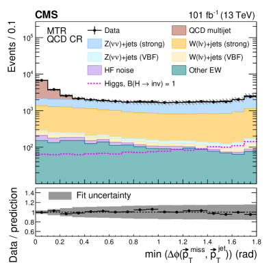
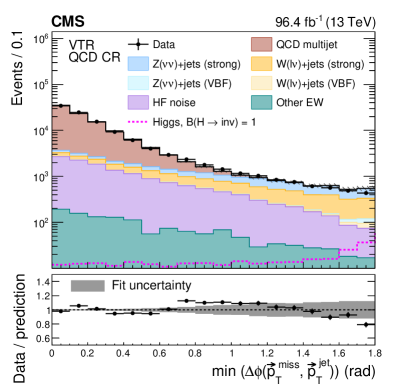
Figure 4: The $\min(\Delta\phi(\ptvecmiss,\vec{p}_{\mathrm{T}}^{\kern 1.0pt\text{jet}}))$ distribution in data from 2017 and 2018, and contributions from $\PV\text{+jets}$, diboson plus top quark processes, HF noise, and QCD multijet events for the MTR (left) and VTR (right) categories. The uncertainty band shows the uncertainty from the fit used to determine the normalization of the QCD multijet template in the corresponding SR. The yields from the 2017 and 2018 samples are summed and the correlations between their uncertainties are neglected.

The function $f_{\text{QCD}}(x)$ provides an estimate of the QCD multijet template normalization, $N$, in the SR via

$$N=\int_{X}^{\pi}f_{\text{QCD}}(x)\,\rd{x},$$ (3)

where $X=0.5$ for the MTR categories and $X=1.8$ for the VTR categories. An uncertainty in $N$ is derived by generating, and then refitting, pseudodata to extract the standard deviation of $\log N$. This uncertainty includes the statistical uncertainty in the fit for the QCD multijet normalization and the uncertainty in the templates from simulation used to subtract the backgrounds due to the limited number of simulated events.

0.6 Sources of uncertainty

Several sources of systematic uncertainty affect the predictions of the signal and background components. They are separated into two categories, experimental and theoretical sources. Their effect is propagated either directly to the yields expected in the SR (for signal and backgrounds estimated directly from simulation), or to the transfer factors (for the $\PV\text{+jets}$ processes estimated from the CRs).

0.6.1 Experimental uncertainties

The reconstruction and identification efficiencies of electrons, photons, muons, candidates, and -tagged jets have been measured in both data and simulation [CMS:2020uim, CMS:2018rym, CMS:2018jrd, Sirunyan:2017ezt]. The simulated events are corrected by scale factors, which are usually dependent on the and $\eta$ of the object, and have associated systematic uncertainties. The scale factors, and their uncertainties, are also propagated when vetoing events with identified objects. For the electrons and muons, when different working points are chosen between leptons selected in the CRs and vetoed in the SR, the corresponding uncertainties are kept uncorrelated. All these uncertainties are correlated between the MTR and VTR categories. Except for the muons, where the dominant source of systematic uncertainty comes from the experimental method employed, these uncertainties are considered uncorrelated between the 2017 and 2018 data sets.

The effects of the jet energy scale (JES) and jet energy resolution (JER) uncertainties are studied explicitly by varying them by one standard deviation [Khachatryan:2016kdb], propagating the changes to the accordingly, and checking the impact on the transfer factors for the $\PV\text{+jets}$ processes as functions of $m_{\mathrm{jj}}$. For the signal and the minor backgrounds, the impact is studied on the simulated yields in the SR as a function of $m_{\mathrm{jj}}$, with a fit procedure to remove the statistical contribution in the less-populated high-$m_{\mathrm{jj}}$ bins. The JER uncertainties impact the signal yields by 4–9 (2–15)%, increasing with $m_{\mathrm{jj}}$, for VBF ($\Pg\Pg\PH$) production. The impacts of the JES uncertainties are 5–25 (7–35)%, increasing with $m_{\mathrm{jj}}$, for the VBF ($\Pg\Pg\PH$) process. Eleven independent JES sources are considered, with partial correlations between the 2017 and 2018 data sets. The dominant source is the $\eta$ dependence of the corrections. The corrections become particularly large for forward jets, which explains the large increase at high $m_{\mathrm{jj}}$. The JER uncertainties are uncorrelated between the two data-taking years. Both the JER and JES uncertainties are correlated between the MTR and VTR categories.

Simulated events are weighted to match the distribution of reconstructed vertices to the distribution observed in the data. An uncertainty associated with this procedure is obtained by varying the total inelastic $\Pp\Pp$ cross section by $\pm 5\%$ [CMS:2018mlc], and repeating the background estimation procedure. This uncertainty is correlated across categories and data sets.

The trigger efficiencies are measured in both data and simulation, and a scale factor is extracted. For the signal triggers, the scale factor is parameterized as a function of the . The associated systematic uncertainty partially cancels in the transfer factors between the muon CRs and the SR. The associated uncertainty is uncorrelated across categories as different triggers are used, but partially correlated between years. For the electron CRs, the scale factor is parameterized as a function of the lepton and $\eta$, and the impact of the uncertainties is propagated to the corresponding expectations in the SR. The uncertainty in the electron trigger scale factor is uncorrelated between years but correlated across categories.

The uncertainty in the integrated luminosity of the 2017 (2018) data set is 2.3% [CMS:2018elu] (2.5% [CMS:2019jhq]). When combined together with the 2016 data set [CMS:2021xjt], the uncertainty is reduced to 1.6%. The improvement in the precision reflects the (uncorrelated) time evolution of some systematic effects. Eight independent sources are identified to take into account the correlations across data sets. These uncertainties are considered correlated between categories.

0.6.2 Theoretical uncertainties

The uncertainties in the $\Pg\Pg\PH$ and VBF predictions due to PDFs and renormalization and factorization scale variations are taken from Ref. [deFlorian:2016spz]. For the $\Pg\Pg\PH$ process, an additional uncertainty of 40% is assigned to take into account the limited knowledge of the $\Pg\Pg\PH$ production cross section in association with two or more jets, as well as the uncertainty in the prediction of the $\Pg\Pg\PH$ differential cross section for large Higgs boson , $\pt^{\PH}>250\GeV$, following the recipe described in Ref. [Sirunyan:2018owy]. The uncertainties in the signal acceptance due to the choice of the PDF set, and the renormalization and factorization scales, are evaluated independently for the different signal processes [Sirunyan:2018owy], and are treated as independent nuisance parameters in the fit.

Some of the theoretical uncertainties in the $\PV\text{+jets}$ and $\Pgg\text{+jets}$ processes are expected to mostly cancel in the ratio of the () to processes. The uncertainties are estimated using the strong production, and applied to both the VBF and strong production processes. As a conservative choice, for the pQCD NLO corrections, the renormalization and factorization scales are varied independently by a factor of two. They are also varied independently for the $\PW(\Pell\PGn)\text{+jets}$ and $\PZ(\PGn\PAGn)\text{+jets}$ processes. The maximum variation in the ratio of the $\PW(\Pell\PGn)\text{+jets}$ to $\PZ(\PGn\PAGn)\text{+jets}$ yields, per $m_{\mathrm{jj}}$ bin, is taken as the uncertainty. The maximum variation is generally given by that of the process. Uncertainties in the PDFs are directly propagated to the ratio of $\PW(\Pell\PGn)\text{+jets}$ to $\PZ(\PGn\PAGn)\text{+jets}$ in a correlated way, and are also applied per $m_{\mathrm{jj}}$ bin. The full EW correction is taken as an additional uncertainty in the ratio of $\PW(\Pell\PGn)\text{+jets}$ ($\Pgg\text{+jets}$) to $\PZ(\PGn\PAGn)\text{+jets}$ for the strong production of those processes, and is assumed to be uncorrelated between $m_{\mathrm{jj}}$ bins. The theoretical uncertainties are assumed uncorrelated between the VBF- and strong-produced $\PV\text{+jets}$ processes, as well as between the MTR and VTR categories.

All theoretical uncertainty sources are fully correlated between years.

0.7 Results

A binned maximum likelihood fit is performed simultaneously across the SR and all CRs in both categories and for both data sets. In the fit, one parameter per bin $i$ of the $m_{\mathrm{jj}}$ distribution, for each category and year, is left freely floating. This parameter represents the expected rate of the background from the strong production of $\PZ(\PGn\PAGn)\text{+jets}$ events, and it is labelled $\kappa_{i}\smash[b]{{}^{\PGn\PAGn}}$. The $m_{\mathrm{jj}}$ distribution is binned in the same way as in Ref. [Sirunyan:2018owy]. This binning has been found to be optimal for the 2017 and 2018 data sets as well. Similar to the method described in Ref. [Sirunyan:2018owy], the likelihood function is defined as:

$$\mathcal{L}(\mu,\kappa\smash[b]{{}^{\PGn\PAGn}},\boldsymbol{\theta})= \prod_{i}\mathrm{P}\left(d_{i}\Big{|}B_{i}(\boldsymbol{\theta})+\PZ_{i}(\kappa_{i}\smash[b]{{}^{\PGn\PAGn}})+\PW_{i}(\kappa_{i}\smash[b]{{}^{\PGn\PAGn}},\boldsymbol{\theta})+\mu S_{i}(\boldsymbol{\theta})\right)$$ (4)

$$\prod_{\mathrm{CR}}\left(\prod_{i}\mathrm{P}\left(d^{\mathrm{CR}}_{i}\Big{|}B^{\mathrm{CR}}_{i}(\boldsymbol{\theta})+\PV_{i}^{\mathrm{CR,strong}}(\kappa_{i}\smash[b]{{}^{\PGn\PAGn}},\boldsymbol{\theta})+\PV_{i}^{\mathrm{CR,VBF}}(\kappa_{i}\smash[b]{{}^{\PGn\PAGn}},\boldsymbol{\theta})\right)\right)$$

$$\prod_{j}\mathrm{P}(\theta_{j}),$$

$$\PZ_{i}(\kappa_{i}\smash[b]{{}^{\PGn\PAGn}})= (1+Z^{\frac{\mathrm{VBF}}{\mathrm{strong}}}_{i})\kappa_{i}\smash[b]{{}^{\PGn\PAGn}},$$

$$\PW_{i}(\kappa_{i}\smash[b]{{}^{\PGn\PAGn}},\boldsymbol{\theta})= (f^{\PW/\PZ\mathrm{,strong}}_{i}(\boldsymbol{\theta})+Z^{\frac{\mathrm{VBF}}{\mathrm{strong}}}_{i}f^{\PW/\PZ\mathrm{,VBF}}_{i}(\boldsymbol{\theta}))\kappa_{i}\smash[b]{{}^{\PGn\PAGn}},$$

$$\PV_{i}^{\mathrm{CR,strong}}(\kappa_{i}\smash[b]{{}^{\PGn\PAGn}},\boldsymbol{\theta})= C^{\mathrm{CR,strong}}_{i}(\boldsymbol{\theta})R^{\mathrm{CR,strong}}_{i}(\boldsymbol{\theta})\kappa_{i}\smash[b]{{}^{\PGn\PAGn}},$$

$$\PV_{i}^{\mathrm{CR,VBF}}(\kappa_{i}\smash[b]{{}^{\PGn\PAGn}},\boldsymbol{\theta})= C^{\mathrm{CR,VBF}}_{i}(\boldsymbol{\theta})Z^{\frac{\mathrm{VBF}}{\mathrm{strong}}}_{i}R^{\mathrm{CR,VBF}}_{i}(\boldsymbol{\theta})\kappa_{i}\smash[b]{{}^{\PGn\PAGn}},$$

where ${\mathrm{P}(x|y)=y^{x}\re^{-y}/x!}$, and $d^{\mathrm{CR}}_{i}$ and $d_{i}$ are the observed number of events in each bin $i$ of the $m_{\mathrm{jj}}$ distribution in each of the CRs and in the SR, respectively. The index $i$ runs over the $m_{\mathrm{jj}}$ bins in the two years and all categories. The symbol $\boldsymbol{\theta}$ refers to constrained nuisance parameters used for the modelling of the systematic uncertainties. The signal term $S_{i}$ represents the expected signal prediction from the sum of the main Higgs boson production mechanisms ($\Pg\Pg\PH$, VBF, $\PV\PH$, $\PQt{}\PQt{}\PH$) assuming the cross sections predicted in the SM. The parameter $\mu=(\sigma_{\PH}/\sigma_{\PH}^{\mathrm{SM}}){\mathcal{B}(\PH\to\text{inv})}$ denotes the signal strength parameter, and is also left freely floating in the fit.

In a given bin, the $\PV\text{+jets}$ background yields expected in the SR are obtained from transfer factors relating the yields in the different CRs to the yields in the SR, separately for the VBF and strong production processes. These transfer factors are denoted $R^{\mathrm{CR,proc}}_{i}(\boldsymbol{\theta})$, where “proc” can be strong or VBF, and are obtained from the simulation. For the single-lepton (dilepton) CRs, the factors $R^{\mathrm{CR,proc}}_{i}(\boldsymbol{\theta})$ refer to the ratio of $\PW\text{+jets}$ ($\PZ\text{+jets}$) yields from the corresponding CR to the SR. In the photon CR, which is only available in the MTR category, $R^{\mathrm{CR,proc}}_{i}(\boldsymbol{\theta})=1$.

In addition, transfer factors are defined between the () and the processes, separately for the VBF and strong production processes. These transfer factors are denoted as $f^{\PW/\PZ\mathrm{,proc}}_{i}(\boldsymbol{\theta})$ ($f^{\Pgg/\PZ\mathrm{,proc}}_{i}(\boldsymbol{\theta})$), where “proc” can be strong or VBF. Finally, a transfer factor, denoted as $Z^{\frac{\mathrm{VBF}}{\mathrm{strong}}}_{i}$, relates the VBF production to the strong production of $\PZ(\PGn\PAGn)\text{+jets}$. The factors $C^{\mathrm{CR,strong}}_{i}(\boldsymbol{\theta})$ and $C^{\mathrm{CR,VBF}}_{i}(\boldsymbol{\theta})$ are dependent on the nature of the CR, with $C^{(\Pe\Pe,\PGm\PGm)\mathrm{,proc}}_{i}=1$, $C^{(\Pe,\PGm)\mathrm{,proc}}_{i}=f^{\PW/\PZ\mathrm{,proc}}_{i}(\boldsymbol{\theta})$, and $C^{\Pgg\mathrm{,proc}}_{i}=f^{\Pgg/\PZ\mathrm{,proc}}_{i}(\boldsymbol{\theta})$.

The contributions from subleading backgrounds in each region are estimated directly from simulation and they are denoted by $B^{\mathrm{CR}}_{i}(\boldsymbol{\theta})$ in the CRs, and $B_{i}(\boldsymbol{\theta})$ in the SR.

Systematic uncertainties are modelled as constrained nuisance parameters ($\boldsymbol{\theta}$), with a log-normal distribution for those that affect the overall normalization of a given process, and Gaussian priors for those that directly affect the transfer factors, indicated by $\mathrm{P}(\theta_{j})$ in Eq. (4). The impact on the transfer factors of each of the uncertainties described in Section 0.6 is summarized in Table 0.7.

Experimental and theoretical sources of systematic uncertainty in the $\PV\text{+jets}$ transfer factors. The second column indicates which ratio a given source of uncertainty is applied to. The impact on $m_{\mathrm{jj}}$ is given in the 3rd column, as a single value if no dependence on $m_{\mathrm{jj}}$ is observed, or as a range. When a range is shown, the uncertainty increases with the value of $m_{\mathrm{jj}}$. The quoted uncertainty values represent the absolute value of the relative change in the transfer factor corresponding to a variation of ${\pm}1$ standard deviation in the systematic uncertainty, or equivalently to a variation of ${\pm}1$ in the corresponding nuisance parameter $\theta$ in Eq. (4). l l c Source of uncertainty Ratios Uncertainty vs. $m_{\mathrm{jj}}$
Theoretical uncertainties
Ren. scale $\PV\text{+jets}$ (VBF) $f^{\PW/\PZ\mathrm{,VBF}}_{i}$ 7.5%
Ren. scale $\PV\text{+jets}$ (strong) $f^{\PW/\PZ\mathrm{,strong}}_{i}$ 8.2%
Fac. scale $\PV\text{+jets}$ (VBF) $f^{\PW/\PZ\mathrm{,VBF}}_{i}$ 1.5%
Fac. scale $\PV\text{+jets}$ (strong) $f^{\PW/\PZ\mathrm{,strong}}_{i}$ 1.3%
PDF $\PV\text{+jets}$ (VBF) $f^{\PW/\PZ\mathrm{,VBF}}_{i}$ 0%
PDF $\PV\text{+jets}$ (strong) $f^{\PW/\PZ\mathrm{,strong}}_{i}$ 0%
NLO EW corr. $\PV\text{+jets}$ (strong) $f^{\PW/\PZ\mathrm{,strong}}_{i}$ 0.5%
Ren. scale $\Pgg\text{+jets}$ (VBF) $f^{\Pgg/\PZ\mathrm{,VBF}}_{i}$ 6–10%
Ren. scale $\Pgg\text{+jets}$ (strong) $f^{\Pgg/\PZ\mathrm{,strong}}_{i}$ 6–10%
Fac. scale $\Pgg\text{+jets}$ (VBF) $f^{\Pgg/\PZ\mathrm{,VBF}}_{i}$ 2.5%
Fac. scale $\Pgg\text{+jets}$ (strong) $f^{\Pgg/\PZ\mathrm{,strong}}_{i}$ 2.5%
PDF $\Pgg\text{+jets}$ (VBF) $f^{\Pgg/\PZ\mathrm{,VBF}}_{i}$ 2.5%
PDF $\Pgg\text{+jets}$ (strong) $f^{\Pgg/\PZ\mathrm{,strong}}_{i}$ 2.5%
NLO EW corr. $\Pgg\text{+jets}$ $f^{\Pgg/\PZ\mathrm{,strong}}_{i}$ 3%
Experimental uncertainties
Electron reco. eff. $R^{\mathrm{CR,proc}}_{i}$, CR$=$$\PZ(\Pe\Pe)$ or $\PW(\Pe\PGn)$ $\approx$0.5% (per lepton)
Electron id. eff. $R^{\mathrm{CR,proc}}_{i}$, CR$=$$\PZ(\Pe\Pe)$ or $\PW(\Pe\PGn)$ $\approx$1% (per lepton)
Muon id. eff. $R^{\mathrm{CR,proc}}_{i}$, CR$=$$\PZ(\PGm\PGm)$ or $\PW(\PGm\PGn)$ $\approx$0.5% (per lepton)
Muon iso. eff. $R^{\mathrm{CR,proc}}_{i}$, CR$=$$\PZ(\PGm\PGm)$ or $\PW(\PGm\PGn)$ $\approx$0.1% (per lepton)
Photon id. eff. $f^{\Pgg/\PZ\mathrm{,proc}}_{i}$ 5%
Electron veto (reco) $f^{\PW/\PZ\mathrm{,proc}}_{i}$, $R^{\mathrm{CR,proc}}_{i}$, CR$=$$\PW(\Pell\PGn)$ $\approx$1.5 (1)% for VBF (strong)
Electron veto (id) $f^{\PW/\PZ\mathrm{,proc}}_{i}$, $R^{\mathrm{CR,proc}}_{i}$, CR$=$$\PW(\Pell\PGn)$ $\approx$2.5 (2)% for VBF (strong)
Muon veto $f^{\PW/\PZ\mathrm{,proc}}_{i}$, $R^{\mathrm{CR,proc}}_{i}$, CR$=$$\PW(\Pell\PGn)$ $\approx$0.5%
veto $f^{\PW/\PZ\mathrm{,proc}}_{i}$, $R^{\mathrm{CR,proc}}_{i}$, CR$=$$\PW(\Pell\PGn)$ $\approx$1%
Electron trigger $R^{\mathrm{CR,proc}}_{i}$, CR$=$$\PZ(\Pe\Pe)$ or $\PW(\Pe\PGn)$ $\approx 1\%$
trigger $R^{\mathrm{CR,proc}}_{i}$, CR$=$$\PZ(\PGm\PGm)$ or $\PW(\PGm\PGn)$ $\approx 2\%$
Photon trigger $f^{\Pgg/\PZ\mathrm{,proc}}_{i}$ 1%
JES $f^{\PW/\PZ\mathrm{,proc}}_{i}$ 1–2%
$R^{\mathrm{CR,proc}}_{i}$, CR$=$$\PW(\Pe\PGn)$ or $\PW(\PGm\PGn)$ 1.0–1.5%
$R^{\mathrm{CR,proc}}_{i}$, CR$=$$\PZ(\Pe\Pe)$ or $\PZ(\PGm\PGm)$ 1%
$f^{\Pgg/\PZ\mathrm{,proc}}_{i}$ 3%
JER $f^{\PW/\PZ\mathrm{,proc}}_{i}$ 1.0–2.5%
$R^{\mathrm{CR,proc}}_{i}$, CR$=$$\PW(\Pe\PGn)$ or $\PW(\PGm\PGn)$ 1.0–1.5%
$R^{\mathrm{CR,proc}}_{i}$, CR$=$$\PZ(\Pe\Pe)$ or $\PZ(\PGm\PGm)$ 1%
$f^{\Pgg/\PZ\mathrm{,proc}}_{i}$ 1–4%

In the following, the expected background yields used as input to the fit procedure are denoted as “prefit”, while the yields after a fit to the CRs, or the CRs and SR, are denoted as “CR-postfit”, or “postfit”, respectively.

The results are presented for the MTR and VTR categories separately. They are shown separately for the 2017 and 2018 data sets when presenting the transfer factors, and for the data sets added together otherwise. The corresponding figures and tables split into individual control regions and data-taking periods are available in Appendix LABEL:app:suppMat.

All results are obtained from a combined fit across all categories and data sets.

For the maximum likelihood fit, the different data sets and categories are treated separately. The final results are obtained from a fit using the combined likelihood function including all categories and data sets, which takes into account nuisance correlations.

0.7.1 Control regions for the MTR category

The ratio of dilepton to single-lepton events is studied to validate the predictions from simulation and uncertainties used to model the ratio of $\PZ\text{+jets}$ to $\PW\text{+jets}$ events in the SR (parameters $f^{\PW/\PZ\mathrm{,proc}}_{i}(\boldsymbol{\theta})$ in Eq. (4)). The prefit ratio between the number of $\PZ\text{+jets}$ and $\PW\text{+jets}$ events in the CRs in bins of $m_{\mathrm{jj}}$ is shown in Fig. 5 (upper row) for the 2017 (left) and 2018 (right) data sets. The prediction is compared to the ratio of observed data yields, from which the estimates of minor background processes have been subtracted. The CR-postfit results are shown together with the prefit ratio. A reasonable agreement is observed between data and simulation, with differences in most bins covered by the systematic uncertainties listed in Table 0.7. In 2017, the simulation predicts a lower ratio than observed in data. The compatibility of the data with the prefit prediction is measured, in this particular category and year only, using a $\chi^{2}$ test accounting for correlations between the 2017 MTR CRs and each $m_{\mathrm{jj}}$ bin. This test indicates that there is a local discrepancy of approximately two standard deviations. The disagreement is attributed to the $\PZ\text{+jets}$ regions with low event yields, and is partially compensated in the fit through the movement of nuisance parameters representing uncertainties such as the renormalization and factorization scales. The significance of the discrepancy is low and none of the nuisance parameters move by more than one standard deviation from their prefit value in the combined fit across all categories and years. The $p$-value [pvalue] for the 2017 data set in the MTR category after the combined fit is 38.4%, and it is 37.0% for all categories when combining the 2017 and 2018 data sets. Closure tests have also been performed comparing the decays to electrons or muons separately for the and CRs, again showing reasonable agreement between data and simulation.

The ratio of photon to dilepton events is also studied to validate the predictions from simulation and uncertainties used to model the ratio of $\Pgg\text{+jets}$ to $\PZ\text{+jets}$ events in the SR (parameters $f^{\Pgg/\PZ\mathrm{,proc}}_{i}(\boldsymbol{\theta})$ in Eq. (4)). The prefit and CR-postfit ratios between the number of events in the $\Pgg\text{+jets}$ over $\PZ\text{+jets}$ CRs in bins of $m_{\mathrm{jj}}$ are shown in Fig. 5 (lower row) for the 2017 (left) and 2018 (right) data sets.

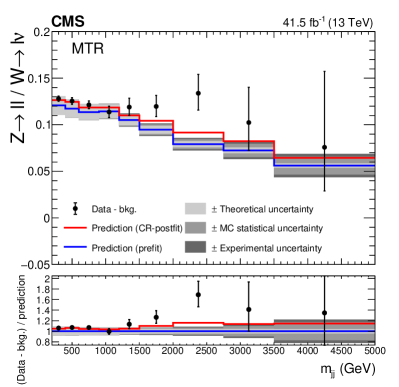
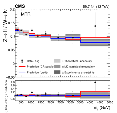
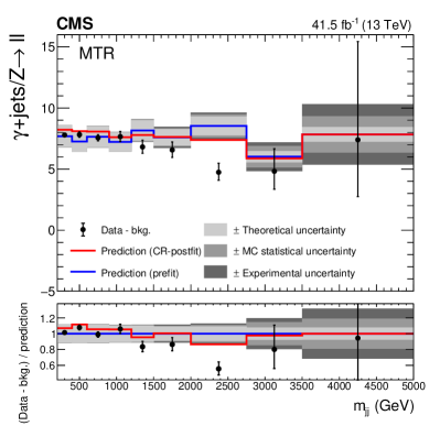
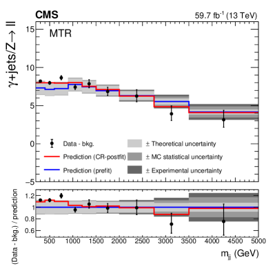
Figure 5: Comparison between data and simulation for the $\PZ(\Pell\Pell)\text{+jets}$/$\PW(\Pell\PGn)\text{+jets}$ (upper row) and $\Pgg\text{+jets}$/$\PZ(\Pell\Pell)\text{+jets}$ (lower row) prefit and CR-postfit ratios, as functions of $m_{\mathrm{jj}}$, for the MTR category using the 2017 (left) and 2018 (right) event samples. The minor backgrounds (bkg.) in each CR are subtracted from the data using estimates from simulation. The grey bands include the theoretical and experimental systematic uncertainties listed in Table 0.7, as well as the statistical uncertainty in the simulation.

The prediction is compared to the ratio of observed data yields, from which the estimates of minor background processes have been subtracted. A similar observation can be made for the 2017 MTR category as for the $\PZ\text{+jets}$ over $\PW\text{+jets}$ ratio. This effect is again attributed to the $\PZ\text{+jets}$ CRs with low event yields.

The $m_{\mathrm{jj}}$ distributions in data in the dilepton and single-lepton CRs, along with the postfit estimates of the background contributions, are shown in Fig. 6.

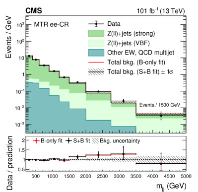
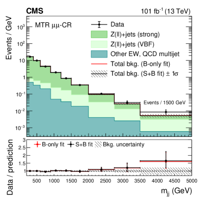
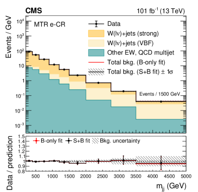
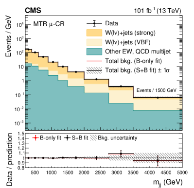
Figure 6: The postfit $m_{\mathrm{jj}}$ distributions in the dielectron (upper left), dimuon (upper right), single-electron (lower left), and single-muon (lower right) CR for the MTR category, showing the summed 2017 and 2018 data samples and the background processes. The background contributions are estimated from the fit to the data described in the text (S+B fit). The total background (bkg.) estimated from a fit assuming ${\mathcal{B}(\PH\to\text{inv})}=0$ (B-only fit) is also shown. The yields from the 2017 and 2018 samples are summed and the correlations between their uncertainties are neglected. The last bin of each distribution integrates events above the bin threshold divided by the bin width.

Similar distributions in the photon CR are shown in Fig. 7.

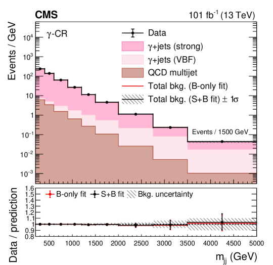
Figure 7: The postfit $m_{\mathrm{jj}}$ distribution in the photon CR for the MTR category, showing the summed 2017 and 2018 data samples and the background processes. The background contributions are estimated from the fit to the data described in the text (S+B fit). The total background (bkg.) estimated from a fit assuming ${\mathcal{B}(\PH\to\text{inv})}=0$ (B-only fit) is also shown. The yields from the 2017 and 2018 samples are summed and the correlations between their uncertainties are neglected. The last bin of each distribution integrates events above the bin threshold divided by the bin width.

The total background estimated from a fit assuming ${\mathcal{B}(\PH\to\text{inv})}=0$ is also shown. The distributions show the sum of the 2017 and 2018 data sets in each region. The postfit predictions are in good agreement with the data within one standard deviation for most of the bins, with discrepancies of just over one standard deviation in the dielectron MTR CR for two bins at $m_{\mathrm{jj}}\approx 2\TeV$. As discussed previously in the context of the validation of the $\PZ\text{+jets}$ over $\PW\text{+jets}$ and the $\Pgg\text{+jets}$ over $\PZ\text{+jets}$ ratios in the CRs, the prefit disagreement observed in the 2017 MTR is partially compensated by the nuisance parameters in the fit, resulting in an overall $p$-value of 37.0%.

0.7.2 Control regions for the VTR category

The prefit and CR-postfit ratios between the number of $\PZ\text{+jets}$ and $\PW\text{+jets}$ events in the CRs in bins of $m_{\mathrm{jj}}$ are shown in Fig. 8. The predictions from simulated events are found to model the data in all bins, within the quoted uncertainties.

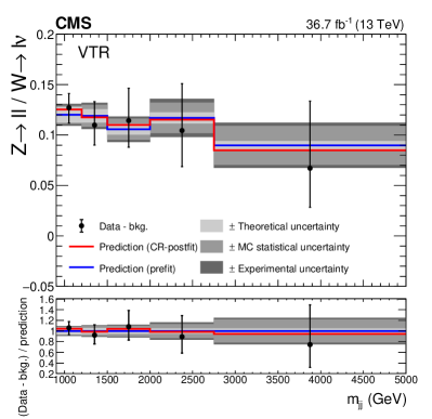
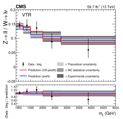
Figure 8: Comparison between data and simulation for the $\PZ(\Pell\Pell)\text{+jets}$/$\PW(\Pell\PGn)\text{+jets}$ prefit and CR-postfit ratios, as functions of $m_{\mathrm{jj}}$, for the VTR category in the 2017 (left) and 2018 (right) data samples. The minor backgrounds (bkg.) in each CR are subtracted from the data using estimates from simulation. The grey bands include the theoretical and experimental systematic uncertainties listed in Table 0.7, as well as the statistical uncertainty in the simulation.

The $m_{\mathrm{jj}}$ distributions in the dilepton and single-lepton CRs are shown in Fig. 9, along with the CR-postfit and postfit estimates. Again, a good agreement between the data and the predictions is shown, within the uncertainties.

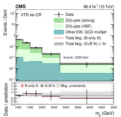
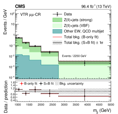
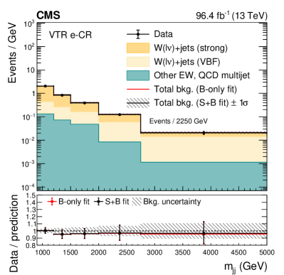
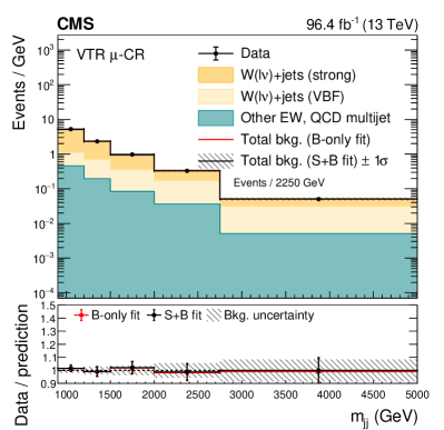
Figure 9: The postfit $m_{\mathrm{jj}}$ distributions in the dielectron (upper left), dimuon (upper right), single-electron (lower left), and single-muon (lower right) CRs for the VTR category, showing the summed 2017 and 2018 data samples and the SM background processes. The background contributions are estimated from the fit to the data described in the text (S+B fit). The total background (bkg.) estimated from a fit assuming ${\mathcal{B}(\PH\to\text{inv})}=0$ (B-only fit) is also shown. The yields from the 2017 and 2018 samples are summed and the correlations between their uncertainties are neglected. The last bin of each distribution integrates events above the bin threshold divided by the bin width.

0.7.3 Signal region fits

The background estimates in the SR are reported for each $m_{\mathrm{jj}}$ bin of the MTR category in Table 0.7.3, and for each $m_{\mathrm{jj}}$ bin of the VTR category in Table 0.7.3. The observed and expected $m_{\mathrm{jj}}$ distributions in the SR are shown in Fig. 10 for the MTR (left) and VTR (right) categories.

[] Expected event yields in each $m_{\mathrm{jj}}$ bin for the different background processes in the SR of the MTR category, summing the 2017 and 2018 samples. The background yields and the corresponding uncertainties are obtained after performing a combined fit across all of the CRs and the SR. The expected signal contributions for the Higgs boson, produced in the non-VBF and VBF modes, decaying to invisible particles with a branching fraction of ${\mathcal{B}(\PH\to\text{inv})}=1$, and the observed event yields are also reported. The yields from the 2017 and 2018 samples are summed and the correlations between their uncertainties are neglected. lccccc $m_{\mathrm{jj}}$ bin range () 200–400 400–600 600–900 900–1200 1200–1500
$\PZ(\PGn\PGn)+\text{jets}$ (strong) $26107.6\pm 82.7$ $15521.0\pm 62.1$ $10747.3\pm 48.8$ $4404.4\pm 25.3$ $1923.4\pm 16.7$
$\PZ(\PGn\PGn)+\text{jets}$ (VBF) $431.3\pm 6.1$ $498.2\pm 6.6$ $620.6\pm 7.0$ $452.0\pm 6.2$ $294.9\pm 5.3$
$\PW(\Pell\PGn)+\text{jets}$ (strong) $13571.4\pm 76.8$ $8293.4\pm 53.0$ $5868.4\pm 43.2$ $2409.6\pm 23.4$ $1053.6\pm 16.1$
$\PW(\Pell\PGn)+\text{jets}$ (VBF) $268.0\pm 10.5$ $301.5\pm 11.3$ $353.5\pm 12.7$ $242.8\pm 8.5$ $163.0\pm 5.9$
$\ttbar$ + single quark $498.8\pm 21.2$ $370.6\pm 15.6$ $275.5\pm 11.8$ $115.3\pm 5.1$ $59.6\pm 2.8$
Diboson $464.9\pm 40.0$ $305.1\pm 26.2$ $246.3\pm 21.3$ $85.4\pm 7.5$ $39.4\pm 3.5$
$\PZ/\Pgg^{*}(\Pell^{+}\Pell^{-})+\text{jets}$ $192.3\pm 4.4$ $126.3\pm 2.9$ $102.0\pm 2.5$ $38.2\pm 1.0$ $16.1\pm 0.5$
Multijet $10.9\pm 2.0$ $10.6\pm 1.9$ $10.4\pm 1.8$ $4.8\pm 0.9$ $2.3\pm 0.4$
HF noise $0.8\pm 0.1$ $35.1\pm 3.0$ $82.7\pm 7.3$ $70.3\pm 6.2$ $28.1\pm 2.5$
$\PQq\PQq\PH(\to\text{inv})$ 130.5 297.0 586.1 571.7 460.5
Other $\PH(\to\text{inv})$ signals 1430.9 1027.1 848.7 414.3 209.5
Total bkg. $41546.0\pm 122.3$ $25461.7\pm 88.2$ $18306.6\pm 71.5$ $7822.8\pm 37.6$ $3580.2\pm 25.1$
Observed 41450 25536 18438 7793 3629
lcccc $m_{\mathrm{jj}}$ bin range () 1500–2000 2000–2750 2750–3500 $>$3500
$\PZ(\PGn\PGn)+\text{jets}$ (strong) $1261.7\pm 12.7$ $462.4\pm 7.4$ $95.6\pm 4.7$ $28.8\pm 1.4$
$\PZ(\PGn\PGn)+\text{jets}$ (VBF) $317.8\pm 6.0$ $197.3\pm 5.3$ $62.1\pm 3.6$ $35.8\pm 2.3$
$\PW(\Pell\PGn)+\text{jets}$ (strong) $704.3\pm 10.9$ $276.7\pm 7.6$ $65.4\pm 4.1$ $23.5\pm 2.4$
$\PW(\Pell\PGn)+\text{jets}$ (VBF) $163.9\pm 6.1$ $111.9\pm 4.6$ $49.4\pm 3.2$ $19.2\pm 1.6$
$\ttbar$ + single quark $38.7\pm 2.2$ $14.9\pm 1.2$ $5.3\pm 0.5$ $1.8\pm 0.2$
Diboson $27.4\pm 2.7$ $7.9\pm 0.8$ $0.6\pm 0.1$ $0.0\pm 0.1$
$\PZ/\Pgg^{*}(\Pell^{+}\Pell^{-})+\text{jets}$ $11.9\pm 0.6$ $4.9\pm 0.3$ $1.5\pm 0.1$ $0.3\pm 0.1$
Multijet $2.1\pm 0.4$ $1.0\pm 0.2$ $0.4\pm 0.1$ $0.2\pm 0.1$
HF noise $56.4\pm 5.0$ $62.2\pm 5.6$ $30.5\pm 2.7$ $20.9\pm 1.8$

$\PQq\PQq\PH(\to\text{inv})$ 539.6 427.2 177.9 118.0
Other $\PH(\to\text{inv})$ signals 161.8 84.7 24.3 11.0

Total bkg. $2584.4\pm 19.8$ $1139.2\pm 14.0$ $310.7\pm 8.3$ $130.6\pm 4.4$

Observed 2623 1142 279 136

[] Expected event yields in each $m_{\mathrm{jj}}$ bin for the different background processes in the SR of the VTR category, summing the 2017 and 2018 samples. The background yields and the corresponding uncertainties are obtained after performing a combined fit across all of the CRs and the SR. The expected signal contributions for the Higgs boson, produced in the non-VBF and VBF modes, decaying to invisible particles with a branching fraction of ${\mathcal{B}(\PH\to\text{inv})}=1$, and the observed event yields are also reported. The yields from the 2017 and 2018 samples are summed and the correlations between their uncertainties are neglected. lccccc $m_{\mathrm{jj}}$ bin range () 900–1200 1200–1500 1500–2000 2000–2750 $>$2750
$\PZ(\PGn\PGn)+\text{jets}$ (strong) $1075.2\pm 14.9$ $444.3\pm 9.4$ $286.5\pm 6.6$ $97.2\pm 3.5$ $38.0\pm 1.9$
$\PZ(\PGn\PGn)+\text{jets}$ (VBF) $132.2\pm 4.1$ $95.2\pm 4.2$ $85.1\pm 4.4$ $56.8\pm 3.7$ $33.6\pm 2.5$
$\PW(\Pell\PGn)+\text{jets}$ (strong) $1048.7\pm 20.8$ $446.4\pm 13.5$ $299.8\pm 11.0$ $139.0\pm 9.1$ $45.1\pm 4.6$
$\PW(\Pell\PGn)+\text{jets}$ (VBF) $114.4\pm 6.7$ $89.9\pm 6.0$ $74.0\pm 5.3$ $53.7\pm 4.4$ $40.5\pm 3.5$
$\ttbar$ + single quark $25.6\pm 1.4$ $14.5\pm 0.9$ $6.5\pm 0.5$ $9.3\pm 0.6$ $4.2\pm 0.8$
Diboson $15.7\pm 1.4$ $7.6\pm 0.8$ $4.2\pm 0.4$ $0.4\pm 0.1$ $0.0\pm 0.1$
$\PZ/\Pgg^{*}(\Pell^{+}\Pell^{-})+\text{jets}$ $31.2\pm 1.0$ $14.5\pm 0.5$ $6.8\pm 0.3$ $4.1\pm 0.2$ $1.6\pm 0.2$
Multijet $0.1\pm 0.1$ $0.1\pm 0.1$ $0.1\pm 0.1$ $0.1\pm 0.1$ $0.0\pm 0.1$
HF noise $30.9\pm 3.0$ $30.4\pm 3.2$ $26.4\pm 2.5$ $48.2\pm 4.8$ $26.0\pm 2.6$
$\PQq\PQq\PH(\to\text{inv})$ 226.7 169.9 195.0 140.9 97.4
Other $\PH(\to\text{inv})$ signals 67.1 33.2 24.9 11.4 5.0
Total bkg. $2474.1\pm 27.0$ $1142.8\pm 18.3$ $789.2\pm 14.8$ $408.7\pm 12.3$ $189.1\pm 7.1$
Observed 2433 1164 780 422 197

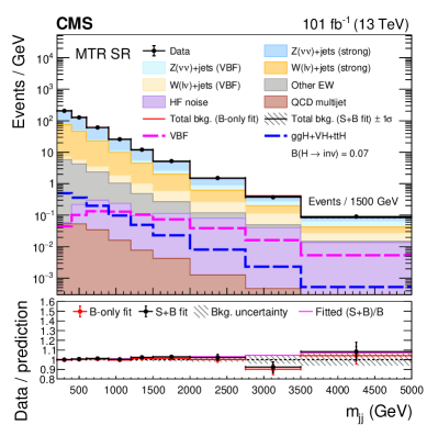
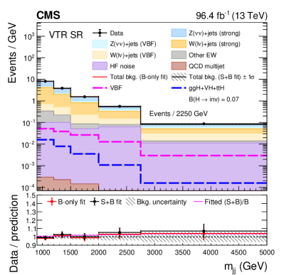
Figure 10: The observed $m_{\mathrm{jj}}$ distribution in the MTR (left) and VTR (right) SR compared with the postfit backgrounds, showing the summed 2017 and 2018 samples. The signal processes are scaled by the fitted value of ${\mathcal{B}(\PH\to\text{inv})}$, shown in the legend. The background contributions are estimated from the fit to the data described in the text (S+B fit). The total background (bkg.) estimated from a fit assuming ${\mathcal{B}(\PH\to\text{inv})}=0$ (B-only fit) is also shown. The yields from the 2017 and 2018 samples are summed and the correlations between their uncertainties are neglected. The last bin of each distribution integrates events above the bin threshold divided by the bin width.

0.7.4 Combination of results

No significant deviations from the SM expectations are observed. The results of this search are interpreted in terms of an upper limit on the product of the Higgs boson production cross section and its branching fraction to invisible particles, $\sigma_{\PH}{\mathcal{B}(\PH\to\text{inv})}$, relative to the predicted cross section assuming SM interactions, $\sigma_{\PH}^{\text{SM}}$. Observed and expected 95% upper limits are computed using an asymptotic approximation of the method detailed in Refs. [Junk:1999kv, Read:2002av], with a profile likelihood ratio test statistic [Cowan:2010js] in which systematic uncertainties are modelled as nuisance parameters following a frequentist approach [CMS-NOTE-2011-005].

Both VBF and non-VBF signal production modes are included, with their relative contributions fixed to the SM prediction within their uncertainties.

Between the 2017 and 2018 data sets, and the two analysis categories (MTR and VTR), the uncertainties are correlated according to the description given in Section 0.6. To combine with the data taken in 2016, the same correlation scheme as between 2017 and 2018 is used, except for the jet energy calibration uncertainties (JES and JER), which are kept fully uncorrelated. The integrated luminosity of the 2016 data set was updated to 36.3to reflect the latest improvements in the luminosity measurement [CMS:2021xjt]. To be consistent with the treatment of the VBF signal in the 2017 and 2018 analyses, the Higgs boson -dependent EW NLO corrections are also applied to the 2016 signal shape. The VBF results obtained with the earlier data sets, namely the data set from 2012 (2015), at $\sqrt{s}=8\,(13)\TeV$, with 19.7 (2.3), from Ref. [Khachatryan:2016whc], are combined taking into account uncertainty correlations where appropriate. Theoretical uncertainties related to signal modelling are correlated for data-taking periods with the same center-of-mass energy. Partial correlations between data sets exist for the uncertainty in the luminosity measurements. All other experimental uncertainties are decorrelated between the run periods before and after 2015. The results of the fit to the data across all data-taking periods are available in Appendix LABEL:app:suppMat.

Constraints on an SM-like Higgs boson

Observed and expected upper limits on $(\sigma_{\PH}/\sigma_{\PH}^{\mathrm{SM}}){\mathcal{B}(\PH\to\text{inv})}$ at 95% are presented in Fig. 11 and Table 0.7.4. The limits are computed for the combination of all data sets, as well as for individual categories and data-taking periods. By itself, the addition of the $\Pgg\text{+jets}$ CR (the addition of the VTR category) improves the expected limits by about 11 (8)% compared with the 2016-like analysis selections. Considered together, the improvements reach about 17% in both years. The upper limits for the individual categories entering the combination are available in Appendix LABEL:app:suppMat.

The combination of the 2017 and 2018 results yields an observed (expected) upper limit of ${{\mathcal{B}(\PH\to\text{inv})}<0.18\,(0.12)}$ at the 95% , assuming an SM Higgs boson with a mass of 125.38 [CMS:2020xrn]. Figure 11 additionally shows a combination with data collected in 2012 and 2015 [Khachatryan:2016whc], and in 2016 [Sirunyan:2018owy]. This combination yields an observed (expected) upper limit of ${{\mathcal{B}(\PH\to\text{inv})}<0.18\,(0.10)}$ at the 95% , which is currently the most stringent limit on ${\mathcal{B}(\PH\to\text{inv})}$.

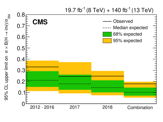
Figure 11: Observed and expected 95% upper limits on $(\sigma_{\PH}/\sigma_{\PH}^{\mathrm{SM}}){\mathcal{B}(\PH\to\text{inv})}$ for all data-taking years considered, as well as their combination, assuming an SM Higgs boson with a mass of 125.38.

The 95% upper limits on $(\sigma_{\PH}/\sigma_{\PH}^{\mathrm{SM}}){\mathcal{B}(\PH\to\text{inv})}$, assuming an SM Higgs boson with a mass of 125.38. The observed and median expected results are shown, along with the 68% and 95% interquartile ranges for each category and for the combinations. l c c c c Category Observed Median expected 65% expected 95% expected
2012–2016 0.33 0.21 [0.15, 0.29] [0.11, 0.39]

VTR 2017 0.57 0.45 [0.32, 0.66] [0.24, 0.94]
VTR 2018 0.44 0.34 [0.24, 0.49] [0.18, 0.69]
VTR 2017+2018 0.40 0.28 [0.20, 0.40] [0.15, 0.56]

MTR 2017 0.25 0.19 [0.14, 0.28] [0.10, 0.40]
MTR 2018 0.24 0.15 [0.11, 0.22] [0.08, 0.31]
MTR 2017+2018 0.17 0.13 [0.09, 0.18] [0.07, 0.25]

all 2017 0.24 0.18 [0.13, 0.26] [0.09, 0.37]
all 2018 0.25 0.15 [0.10, 0.21] [0.08, 0.29]
all 2017+2018 0.18 0.12 [0.08, 0.17] [0.06, 0.23]

2012–2018 0.18 0.10 [0.07, 0.14] [0.05, 0.20]

Figure 12 shows the profile likelihood ratio ($q$) as a function of ${\mathcal{B}(\PH\to\text{inv})}$, for the individual data-taking periods and for their combination. The observed (expected) combined 2012–2018 best fit signal strength is found to be $0.086^{+0.054}_{-0.052}$ ($0.00^{+0.051}_{-0.052}$). Table 0.7.4 summarizes the uncertainties in the measured ${\mathcal{B}(\PH\to\text{inv})}$, separating the contributions from different groups of uncertainties. The systematic uncertainties with the largest impacts in the ${\mathcal{B}(\PH\to\text{inv})}$ measurement are the theoretical uncertainties affecting the $f^{\PW/\PZ\mathrm{,proc}}_{i}$ ratio, followed by the statistical uncertainties in the simulated samples, the trigger uncertainties, jet calibration effects, and the uncertainties in the QCD multijet modelling.

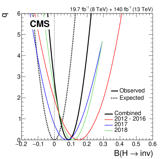
Figure 12: Profile likelihood ratios, as functions of ${\mathcal{B}(\PH\to\text{inv})}$. The observed likelihood scans are reported for the full combination of 2012–2018 data, as well as for the individual years. The expected results for the combination are obtained using an Asimov data set [Cowan:2010js] with ${\mathcal{B}(\PH\to\text{inv})}=0$.

Uncertainty breakdown in ${\mathcal{B}(\PH\to\text{inv})}$. The sources of uncertainty are separated into different groups. Observed and expected results are quoted for the full combination of 2012–2018 data. The expected results are obtained using an Asimov data set [Cowan:2010js] with ${\mathcal{B}(\PH\to\text{inv})}=0$. l c c Group of systematic uncertainties Impact on ${\mathcal{B}(\PH\to\text{inv})}$
Observed Expected
Theory ${}^{+0.026}_{-0.025}$ $\pm 0.024$
Simulated event count $\pm 0.022$ ${}^{+0.021}_{-0.022}$
Triggers ${}^{+0.018}_{-0.019}$ $\pm 0.018$
Jet calibration ${}^{+0.014}_{-0.012}$ $\pm 0.011$
QCD multijet mismodelling $\pm 0.012$ $\pm 0.013$
Leptons/photons/-tagged jets ${}^{+0.011}_{-0.010}$ ${}^{+0.009}_{-0.010}$
Integrated luminosity/pileup $\pm 0.004$ $\pm 0.004$
Other systematic uncertainties ${}^{+0.013}_{-0.009}$ $\pm 0.009$
Statistical uncertainty $\pm 0.028$ $\pm 0.028$

The upper limit on ${\mathcal{B}(\PH\to\text{inv})}$, obtained from the combination of 2012–2018 data, is interpreted in the context of Higgs-portal models of DM interactions, in which a stable DM particle couples to the SM Higgs boson. The interaction between a DM particle and an atomic nucleus may be mediated by the exchange of a Higgs boson, producing nuclear recoil signatures, such as those investigated by direct detection experiments. The sensitivity of these experiments depends mainly on the DM particle mass ($m_{\mathrm{DM}}$). If $m_{\mathrm{DM}}$ is smaller than half of the Higgs boson mass, the partial width of the invisible Higgs boson decay ($\Gamma_{\text{inv}}$) can be translated, within an effective field theory approach, into a spin-independent DM-nucleon elastic scattering cross section, as outlined in Ref. [Djouadi:2011aa]. This translation is performed assuming that the DM candidate is either a scalar or a Majorana fermion, and both the central value and the uncertainty in the dimensionless nuclear form factor $f_{N}$ are taken from the recommendations of Ref. [Hoferichter:2017olk]. The conversion from ${\mathcal{B}(\PH\to\text{inv})}$ to $\Gamma_{\text{inv}}$ uses the relation ${{\mathcal{B}(\PH\to\text{inv})}=\Gamma_{\text{inv}}/(\Gamma_{\mathrm{SM}}+\Gamma_{\text{inv}})}$, where $\Gamma_{\mathrm{SM}}$ is set to 4.07 [Heinemeyer:2013tqa]. We do not perform the translation under the assumption of a vector DM candidate in this paper, since it requires an extended dark Higgs sector, which may lead to modifications of kinematic distributions assumed for the invisibly decaying Higgs boson signal. Figure 13 shows the 90% upper limits on the spin-independent DM-nucleon scattering cross section as a function of $m_{\mathrm{DM}}$, for both the scalar and the fermion DM scenarios. The corresponding 90% upper limit on ${\mathcal{B}(\PH\to\text{inv})}$ is 0.16. These limits are computed at the 90% so that they can be compared with those from direct detection experiments such as XENON1T [Aprile:2018dbl], CRESST-II [Angloher:2015ewa], CDMSlite [Agnese:2015nto], LUX [Akerib:2016vxi], Panda-X 4T [PandaX-4T:2021bab], and DarkSide-50 [Agnes:2018ves], which provide the strongest constraints in the $m_{\mathrm{DM}}$ range probed by this search. The collider-based results complement the direct-detection experiments in the range $m_{\mathrm{DM}}$ smaller than 12 (6), assuming a fermion (scalar) DM candidate.

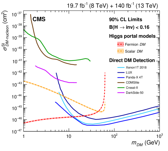
Figure 13: The 90% upper limits on the spin-independent DM-nucleon scattering cross section in Higgs-portal models, assuming a scalar (dashed orange) or fermion (dashed red) DM candidate. Limits are computed as functions of $m_{\mathrm{DM}}$ and are compared to those from the XENON1T [Aprile:2018dbl], CRESST-II [Angloher:2015ewa], CDMSlite [Agnese:2015nto], LUX [Akerib:2016vxi], Panda-X 4T [PandaX-4T:2021bab], and DarkSide-50 [Agnes:2018ves] experiments, which are shown as solid lines.

0.8 Summary

A search for the Higgs boson () decaying invisibly, produced in the vector boson fusion mode, is performed with 101of proton-proton collisions delivered by the LHC at $\sqrt{s}=13\TeV$ and collected by the CMS detector during 2017–2018. Building upon the previously published results, an additional category targeting events at lower Higgs boson transverse momentum is added. An additional highly populated control region, based on production of a photon associated with jets, is used to constrain the dominant irreducible background from invisible decays of a boson produced in association with jets. Compared with the strategy of the previously published analysis, these additions improve the expected limits by approximately 17%. The observed (expected) upper limit on the invisible branching fraction of the Higgs boson, ${\mathcal{B}(\PH\to\text{inv})}$, is found to be $0.18$ ($0.12$) at the 95% confidence level (), assuming the standard model production cross section. The results are combined with previous measurements in the vector boson fusion topology, for total integrated luminosities of 19.7at $\sqrt{s}=8\TeV$ and 140at $\sqrt{s}=13\TeV$, yielding an observed (expected) upper limit of $0.18$ ($0.10$) at the 95% . This is currently the most stringent limit on ${\mathcal{B}(\PH\to\text{inv})}$. Finally, the results are interpreted in the context of Higgs-portal models. The 90% upper limits on the spin-independent dark-matter-nucleon scattering cross section obtained from the observed LHC data collected during 2012–2018 complement the direct detection experiments in the range of dark matter particle masses smaller than 12 (6), assuming a fermion (scalar) dark matter candidate.