Grad2Task: Improved Few-shot Text Classification Using Gradients for Task Representation

Abstract

Large pretrained language models (LMs) like BERT have improved performance in many disparate natural language processing (NLP) tasks. However, fine tuning such models requires a large number of training examples for each target task. Simultaneously, many realistic NLP problems are "few shot", without a sufficiently large training set. In this work, we propose a novel conditional neural process-based approach for few-shot text classification that learns to transfer from other diverse tasks with rich annotation. Our key idea is to represent each task using gradient information from a base model and to train an adaptation network that modulates a text classifier conditioned on the task representation. While previous task-aware few-shot learners represent tasks by input encoding, our novel task representation is more powerful, as the gradient captures input-output relationships of a task. Experimental results show that our approach outperforms traditional fine-tuning, sequential transfer learning, and state-of-the-art meta learning approaches on a collection of diverse few-shot tasks. We further conducted analysis and ablations to justify our design choices.

1 Introduction

Transformer-based pretrained large-scale language models (LMs) have achieved tremendous success on many NLP tasks [15, 34], but require a large number of in-domain labeled examples for fine-tuning [54]. One approach to alleviate that issue is to fine-tune the model on an intermediate (source) task that is related to the target task. While previous work has focused on this setting for a single source task [33, 50], the problem of transferring from a set of source tasks has not been thoroughly considered. Wang et al. [51] showed that a naïve combination of multiple source tasks may negatively impact target task performance. Additionally, transfer learning methods typically consider the setting where more than a medium (N>100) number of training examples are available for both the source and target tasks.

In this work we develop a method to improve a large pre-trained LM for few-shot text classification problems by transferring from multiple source tasks. While it is possible to directly adapt recent advances in meta-learning developed for few-shot image classification, a unique challenge in the NLP setting is that source tasks do no share the same task structure. Namely, on standard few-shot image classification benchmarks, the training tasks are sampled from a “single” larger dataset, and the label space contains the same task structure for all tasks. In contrast, in text classification tasks, the set of source tasks available during training can range from sentiment analysis to grammatical acceptability judgment. Different source tasks could not only be different in terms of input domain, but also their task structure (i.e. label semantics, and number of output labels).

This challenging problem requires resistance to overfitting due to its few-shot nature and more task-specific adaptation due to the distinct nature among tasks. Fine-tuning based approaches are known to suffer from the overfitting issue and approaches like MAML [17] and prototypical networks (ProtoNet) [41] were not designed to meta-learn from such a diverse collection of tasks. CNAP [37], a conditional neural process [18], explicitly designed for learning from heterogeneous task distributions by adding a task conditional adaptation mechanism is better suited for solving tasks with a shifted task distribution. We design our approach based on the CNAP framework. Compared with CNAP, we use pretrained transformers for text sequence classification instead of convolutional networks for image classification. We insert adapter modules [21] into a pretrained LM to ensure efficiency and maximal parameter-sharing, and learn to modulate those adapter parameters conditioned on tasks, while CNAP learns to adapt the whole feature extractor. Additionally, we use gradient information for task representation as opposed to average input encoding in CNAP, since gradients can capture information from both input and ouput space.

In summary, our main contributions and findings are:

• We propose the use of gradients as features to represent tasks under a model-based meta-learning framework. The gradient features are used to modulate a base learner for rapid generalization on diverse few-shot text classification tasks.

• We use pre-trained BERT with adapter modules [21] as the feature extractor and show that it works better than using only the BERT model on few-shot tasks, while also being more efficient to train as it has much fewer parameters to learn.

• We compare our approach with traditional fine-tuning, sequential transfer learning, and state-of-the-art meta-learning approaches on a collection of diverse few-shot text classification tasks used in [5] and three newly added tasks, and show that our approach achieves the best performance. Our codes are publicly available.

2 Related Work

2.1 Few-shot text classification

There is a wide range of text classification tasks, such as user intent classification, sentiment analysis, among others. Few-shot text classification tasks refer to those that contain novel classes unseen in training tasks and where only a few labeled examples are given for each class [55]. Meta-learning approaches have been proposed for this problem [7, 19, 5]. To increase the amount and diversity of training episodes, previous work trained few-shot learners by semi-supervised learning [40] and self-supervised learning [6]. We compare different meta-learning approaches following the experiment procedures of [5].

2.2 Meta-learning

Metric-based meta-learning approaches [49, 41, 45] try to learn embedding models on which simple classifiers can achieve good performance. Optimization-based approaches [17, 38, 30] are designed to learn good parameter initialization that can quickly adapt to new tasks within a few gradient descent steps. “Black box” or model-based meta-learning approaches use neural networks to embed task information and predict test examples conditioned on the task information [39, 36, 28, 31, 18, 37]. Our approach falls into this third category and is mostly related to CNAP [37]. Compared with CNAP we use a different feature extractor and different mechanisms for modulation, as well as focusing on different problems. An important difference with CNAP is that we use gradient information as features to represent tasks, instead of using average input encoding. Gradient information has also been used to generate task-dependent attenuation of parameter initialization under the MAML framework [4].

2.3 Transfer learning

Our work is also related to transfer learning. Instead of fine-tuning a pretrained language model directly on a target task, Phang et al. [33] and Talmor and Berant [46] showed that intermediate training on data-rich supervised tasks is beneficial for downstream performance. Wang et al. [51] found that there is no guarantee that multi-task learning or intermediate training yields better performance than direct fine-tuning on target tasks. Transferability estimation is the task of predicting whether it is beneficial to transfer from some task to another one. There have been works estimating transferability of NLP tasks based on handcrafted features [8, 23], while data-driven approaches have been studied mainly for computer vision tasks [56, 47, 43, 29].

Task2Vec is a task embedding approach based on the Fisher Information Matrix (FIM) [2]. Transferability between tasks can be easily evaluated by the distance between their task embeddings according to some simple metric. In the NLP domain, given a target task and a predefined set of source tasks, Vu et al. [50] proposed to use task embedding based on FIM to measure task similarity and predict transferability according to the distance between task embeddings. We draw inspiration from this work to use gradients as features for task representation. Instead of one-to-one transfer, our work can be seen as transferring from a set of source tasks to new tasks through meta-learning.

3 Problem Definition

Following the terminologies in meta learning, each task (or episode), $t=(\mathcal{S},\mathcal{Q})$, is specified by a support set (training set) $\mathcal{S}$ and a query set (test set) $\mathcal{Q}$, where $\mathcal{S}=\{(x_{i},y_{i})\}_{i=1}^{|\mathcal{S}|}$, $\mathcal{Q}=\{(x_{i},y_{i})\}_{i=1}^{|\mathcal{Q}|}$, $x_{i}$ is a text sequence and $y_{i}$ is a discrete value corresponding to a class. Different tasks could have different input domains, different numbers of classes, different label space, and so on.

Our goal is to train a text classification model on a set of labeled datasets $\{\mathcal{D}^{s}_{i}\}_{i=1}^{N}$ of $N$ source tasks. The model is expected to achieve good performance on new target tasks after training. For each target task, a small labeled dataset, e.g., five shots for each class, is given for adaptation or fine-tuning and the full test dataset is used for evaluation. Note that when learning on target tasks, we assume no access to the source tasks nor other target tasks. This is different with multi-task learning where target tasks are learned together with source tasks.

4 Model Design

To handle diverse tasks with different structures a single model may not be flexible enough. Thus, for every task, we utilize a task embedding network to capture the task nature and adapt a base model conditioned on the current task. Task-specific adaptation is done by generating shifting and scaling parameters, named adaptation parameters, that are applied on the hidden representations inside the base model. Figure 1 shows an overview of our model architecture, mainly consisting of three parts: a base model denoted by $f$, a task embedding network denoted by $d$, and an adaptation network denoted by $a$.

To make a prediction, our model takes the following steps: 1) given a support set, it uses the base model (Section 4.1) to compute gradients w.r.t. a subset of its parameters to use as input to the task embedding network (Section 4.2), 2) the task embedding network maps these gradients to task representations, 3) layer-wise adaptation networks (Section 4.3) take as input the task representations and output adaptation parameters, and lastly 4) the adaptation parameters are applied to the base model before it predicts on the query set.

The training of our model consists of two stages: 1) we first train the base model episodically as a prototypical network; 2) we then freeze the base model and train the task embedding network and the adaptation network using the same loss function of the first stage (Section 4.4).

Next we introduce our model in details. The list of notations used throughout the paper can be found in Appendix A.

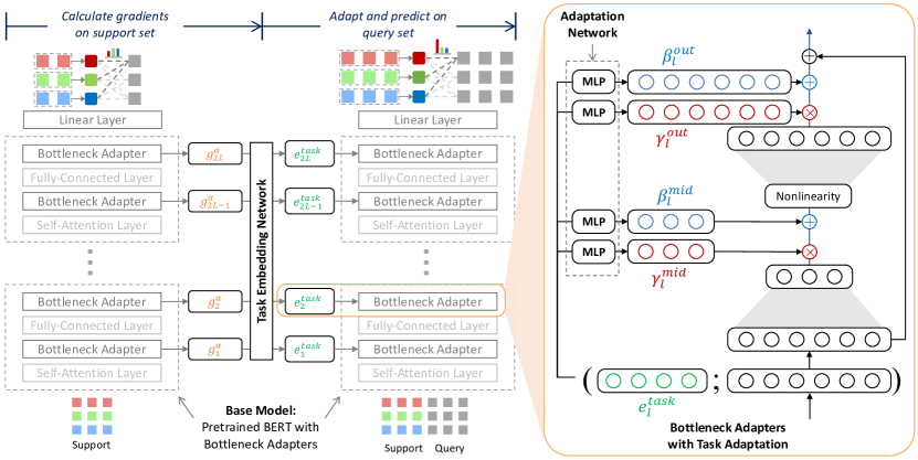
Figure 1: Model architecture overview. Left: The base model contains a pretrained BERT model with bottleneck adapters inserted in each transformer layer and a linear layer stacked on the top. The task embedding network is an RNN-based model that maps gradients from the base model into task representations in a layer-wise fashion, which are used for base model adaptation. Right: The adaptation network contains MLPs that take as input the task representations and intermediate activate inside the base model, and outputs shifting and scaling parameters that are used to adapt the base model. Specifically, given the task embedding for a certain layer, we concatenate it with the input hidden representation to the current layer and map them into four shifting/scaling parameters by four MLP networks, which are applied on the hidden and output representations of the adapter, referred as the auto-regressive adaptation.

4.1 Base Model: BERT & Bottleneck Adapters

Our base model is built upon transformer-based pretrained LMs. We use the pretrained BERT_BASE model throughout this paper, although other transformer-based pretrained LMs are also applicable [35, 25]. Following Houlsby et al. [21], we insert two adapter modules containing bottleneck layers into each transformer layer of BERT. Each bottleneck adapter is denoted as $\alpha_{l},l=1...2L$ where L is the total number of transformer layers in BERT. We use the bottleneck adapters because, first, BERT with adapters are more efficient to train and less vulnerable to overfitting – a desirable property in the few-shot setting. Additionally, this simplifies our goal of using gradients for task representation. It is infeasible to use the gradients of the whole BERT model because the dimensionality is too large. Instead, we compute gradients w.r.t. parameters in these bottleneck layers (< 0.5% of the number of parameters in BERT).

Since text classification is a sequence classification task, we need a pooling method to represent each sequence by a single embedding before the embedding is fed into a classifier. Following Devlin et al. [15], this single embedding is obtained by applying a linear transformation on top of the contextual embedding of the special ‘[CLS]’ token inserted at the beginning of every sequence. We further apply a fully connected layer on top of the BERT output. Together, we name the pretrained BERT with adapters and the last linear layer as the ‘base model’, denoted by $f$. We denote the parameters of the pretrained BERT as $\theta$, bottleneck adapters as $\{\alpha_{l}\}_{l=1}^{2L}$, and linear layer as $\omega$.

For the classifier, we use the ProtoNet classifier  [41]. Given a support set $\mathcal{S}$, a query example $x$ and our base model $f$, a nearest cluster classifier can be described as follows:

$$p^{\text{base}}(y=c\,|\,x) =\mathrm{softmax}(\mathrm{euc}(f(x;\theta,\alpha,\omega),\mu^{c})),$$ (1)

$$\mu^{c} =\frac{1}{|\mathcal{S}^{c}|}\sum_{x_{i}\in\mathcal{S}^{c}}f(x_{i};\theta,\alpha,\omega)$$

where $\mathcal{S}^{c}=\{(x_{i},y_{i})\,|\,(x_{i},y_{i})\in\mathcal{S},y_{i}=c\}$, $\mu^{c}$ is the cluster center in the embedding space for support examples with class $c$, and $\mathrm{euc}$ refers to the Euclidean distance.

4.2 Task Embedding Network for Per-Layer Task Encoding

Our task embedding network, denoted by $d$, is parametrized as a recurrent neural network (RNN) over the layers. We use an RNN to summarize the gradient information from the lower layers so that the higher layers can better adapt to the current tasks. Also, using RNNs can enable parameter sharing across different layers. Concatenating gradients of all layers as input will result in an extremely large task embedding model. The task embedding network takes as input at each layer the gradient information of the adapter parameters at the given layer. Following Achille et al. [2], we use the gradient information defined by the FIM of the base model’s parameters, denoted by $\Theta=\{\theta,\alpha,\omega\}$. The FIM is computed as:

$$F_{\Theta}=\mathbb{E}_{x,y\sim\hat{p}(x)p^{\text{base}}(y\,|\,x)}[\nabla_{\Theta}\log p^{\text{base}}(y\,|\,x)\nabla_{\Theta}\log p^{\text{base}}(y\,|\,x)^{T}]$$ (2)

where $\hat{p}(x)$ is the empirical distribution defined by the dataset. Following Achille et al. [2], we only use the diagonal values of $F_{\Theta}$. We only use those values corresponding to the adapter parameters, denoted by $g^{\alpha}_{l}$ for adapter layer $l$, $l=1\dots 2L$.

Then, the RNN-based task embedding network $d$, parameterized by $\phi$, maps each $g^{\alpha}_{l}$ into a task embedding:

$$e_{l}^{task} =d^{o}(h_{l};\phi),$$ (3)

$$h_{l} =d^{h}(g^{\alpha}_{l},h_{l-1};\phi)$$

where $h_{l}$ is the hidden representation at layer $l$, $e_{l}^{task}$ is the task embedding at layer $l$, $h_{0}$ is the learnable initial RNN hidden state, and $d^{o}$ and $d^{h}$ are the functions of $d$ that produce output and hidden states, respectively.

4.3 Adaptation Network with Auto-Regressive Adaptation

As shown on the right side of Figure 1, at each layer $l$, the adaptation network output four adaptation parameters: $\gamma_{l}^{mid}$ and $\beta_{l}^{mid}$ are scaling and shifting adaptation parameters applied on the hidden representation after the middle layer, and $\gamma_{l}^{out}$ and $\beta_{l}^{out}$ are scaling and shifting adaptation parameters applied on the output hidden representation. The input to the adaptation network at each layer consists of both the task representation and the intermediate activation output by previous adapted layers. Due to the conditioning on previous modulated layers, we refer this adaptation method as auto-regressive adaptation, following Requeima et al. [37].

Starting from the input layer, the adaptation network $a$ produces adaptation parameters for the first adapter layer as follows:

$$\gamma_{1}^{mid},\beta_{1}^{mid},\gamma_{1}^{out},\beta_{1}^{out} =a(e_{1}^{task},x;\psi)$$ (4)

where $x$ is input to the base model. We denote the bottleneck adapter network after modulation as $\alpha^{\prime}$.

For the subsequent layers, the adaptation network takes as input the combination of the task embedding and intermediate activation of the adapted base model, and outputs adaptation parameters as follows:

$$\gamma_{l}^{mid},\beta_{l}^{mid},\gamma_{l}^{out},\beta_{l}^{out} =a(e_{l}^{task},f_{l-1}(x;\theta,\{\alpha^{\prime}_{j}\}_{j=1}^{l-1});\psi),\quad l=2\dots 2L$$ (5)

where $f_{l-1}(x;\theta,\{\alpha^{\prime}_{j}\}_{j=1}^{l-1})$ denotes the intermediate activation before layer $l$ from the base model with the first $l-1$ adapters that have been modulated. Finally, the prediction from our modulated base model is written as:

$$p^{\text{final}}(y=c\,|\,x) =\mathrm{softmax}(\mathrm{euc}(f(x;\theta,\alpha^{\prime},\omega),\mu^{c})),$$ (6)

$$\mu^{c} =\frac{1}{|S^{c}|}\sum_{x_{i}\in\mathcal{S}^{c}}f(x_{i};\theta,\alpha^{\prime},\omega)$$

Notice that the only difference between $p^{\text{final}}(y=c\,|\,x)$ and $p^{\text{base}}(y=c\,|\,x)$ is using $\alpha^{\prime}$ or $\alpha$, i.e. our task-specific modulation.

Our adaptation mechanism is similar with the FiLM layer [32] but different in terms of that here we only apply adaptation on the hidden representation of the “[CLS]”, since only its embedding is used as the sequence embedding. This is analogous to only adapting the the first channel of each hidden representation to a Film layer. We also tried adapting embeddings of all tokens but performance is worse, as shown in Section 6.2.

Input :  $T$: A set of text classification tasks for training. $\mathcal{D}_{i}$: The labeled dataset of each task $i$. The base model trained in the first stage.

Output : $\phi$: Parameters of the task embedding model. $\psi$: Parameters of the adaptation network.

1 while not converge do

2       Sample $M$ episodes $\{t_{i}\}_{i=1}^{M}$, each episode $t_{i}=(\mathcal{S}_{i},\mathcal{Q}_{i}),\mathcal{S}_{i}\subseteq\mathcal{D}_{i},\mathcal{Q}_{i}\subseteq\mathcal{D}_{i}$

3       for $i\leftarrow 1$ to $M$ do

4             for $s\leftarrow 1$ to $S$ do

5                   Sample a few examples for each class from $\mathcal{S}_{i}$ and build prototypes $\{\mu^{c}\}$

6                   Sample another subset of examples $\hat{\mathcal{S}}_{i}\subseteq\mathcal{S}_{i}$

7                   For each $(x_{j},y_{j})\in\hat{\mathcal{S}}_{i}$, sample $y_{j}^{\prime}\sim p^{\text{base}}(y\,|\,x_{j})$ // $p^{\text{base}}$ is given by Equation (1)

8                   $g^{\alpha}_{s}=-\sum_{j=1}^{|\hat{\mathcal{S}}_{i}|}\left(\nabla_{\alpha}\log p^{\text{base}}(y=y_{j}^{\prime}\,|\,x_{j})\right)^{2},(x_{j},y_{j})\in\hat{\mathcal{S}}_{i}$ // calculating gradient

9                   // information as in Equation (2)

10                  

11             end for

12            $g^{\alpha}=\frac{1}{S}\sum_{s=1}^{S}g^{\alpha}_{s}$

13             $e^{task}=d(g^{\alpha};\phi)$ // generating task representation

14             ${\gamma^{in},\beta^{in},\gamma^{out},\beta^{out}}=a(e^{task};\psi)$ // generating adaptation parameters $\ell_{i}=\frac{1}{|\mathcal{Q}_{i}|}\sum_{j=1}^{|\mathcal{Q}_{i}|}-\log p^{\text{final}}(y=y_{j}|x_{j})$ // calculating the loss on query set

15             // $p^{\text{final}}$ is given by Equation (6)    

16       end for

17      ${\{\phi,\psi\}}\leftarrow\{\phi,\psi\}-lr\cdot\nabla_{\{\phi,\psi\}}\sum_{i=1}^{M}\ell_{i}$ // gradient descent on $\phi$ and $\psi$

18 end while

return $\phi,\psi$

Algorithm 1 Training the task embedding network and adaptation network for quick adaptation to new tasks.

4.4 Model Training

Similar with CNAP [37], we train our model in two stages. In the first stage, we train the base model using episodic training [41]. The training algorithm is showed in Appendix B. Given an episode $t=(\mathcal{S},\mathcal{Q})$, the loss is computed as:

$$\ell_{pn}(t)=\frac{1}{|\mathcal{Q}|}\sum_{x_{i}\in\mathcal{Q}}-\log p^{\text{base}}(y_{i}\,|\,x_{i})$$ (7)

During this stage, only the parameters of the bottleneck adapters, layer normalization parameters and the top linear layer are updated while other parameters of the base model are frozen. The parameters are learned by:

$$\alpha^{*},\omega^{*}=\underset{\alpha,\omega}{\arg\min}\mathbb{E}_{t\in T}[\ell_{pn}(t)]$$ (8)

In the second stage, the task embedding network and the adaptation network are trained episodically to generate good quality task embeddings and adaptation parameters for better performance on the query set of each episode. Specifically, as shown in Algorithm 1, we freeze the encoding network and only train the task embedding network $d$ and the adaptation network $a$. In this stage, the frozen base model is used to generate task-specific gradient information and also be adapted to predict the query labels. Same with the first training stage, we also use the ProtoNet loss to train $d$ and $a$ but use the adapted based model. The parameters of the task embedding network $\phi$ and the adaptation network $\psi$ is learned by:

$$\phi^{*},\psi^{*} =\underset{\phi,\psi}{\arg\min}\mathbb{E}_{t\in T}[\ell_{pn}^{\prime}(t)],$$ (9)

$$\quad\ell_{pn}^{\prime}(t) =\frac{1}{|\mathcal{Q}|}\sum_{x_{i}\in\mathcal{Q}}-\log p^{\text{final}}(y_{i}\,|\,x_{i})$$

where the loss is computed based on the modulated model.

5 Experiments and Results

5.1 Experiment setup

We use datasets for training and testing that have different input domains and different numbers of labels. Each dataset appears during either training or testing – not both. Following [5], we use tasks from the GLUE benchmark [52] for training. Specifically, we use WNLI (m/mm), SST-2, QQP, RTE, MRPC, QNLI, and the SNLI dataset [10], to which we refer as our ‘meta-training datasets’. The validation set of each dataset is used for hyperparameter searching and model selection. We train our model and other meta-learning models by sampling episodes from the meta-training tasks. The sampling process first selects a dataset and then randomly selects $k$-shot examples for each class as the support set and another $k$-shot as the query set. As with Bansal et al. [5], the probability of a task being selected is proportional to the square root of its dataset size.

We use the same test datasets as Bansal et al. [5], but also add several new datasets to increase task diversity, namely the Yelp [1] dataset to predict review stars, the SNIPS dataset [13] for intent detection, and the HuffPost [26] dataset for news headline classification. We refer to this set of tasks as our ‘meta-testing datasets’. For each test task and a specific number of shot $k$, ten $k$-shot datasets are randomly sampled. Each time one of the ten datasets is given for model training or fine-tuning, the model is then tested on the full test dataset of the corresponding task. This is in line with real world applications where models built on a small training set are tested on the full test set.

Several test datasets used by Bansal et al. [5] contain very long sentences, but they limited the maximal sequence length to 128 tokens in their experiments. Truncating long sequences beyond the maximal length might lose important information for text classification, leading to noise in the test results. In order to ensure the results can truly reflect text classification, we discard a few datasets used by Bansal et al. [5] that contain many very long sentences.

See Appendix C for more details about the datasets we use. See Appendix G.1 for the results on all datasets used by Bansal et al. [5].

5.2 Few shot text classification results

We use the cased version of the BERT_BASE model for all experiments. We compare our proposed approach with the following approaches:

BERT. The pretrained BERT is simply fine-tuned on the labeled training data of the target task and then evaluated on the corresponding test data. No transfer learning happens with this model.

MT-BERT. The pretrained BERT is first trained on the meta-training tasks via multi-task learning and then fine-tuned and evaluated on each test task.

ProtoNet-BERT. ProtoNet using pretrained BERT plus a linear layer as the feature extractor. The model is trained episodically on the meta-training datasets.

ProtoNet-BN. Similar with ProtoNet-BERT but with adapter modules inserted in the transformer layers. Only the parameters of the adapters, linear layer, and layer normalization layers inside BERT are updated during training. The model is trained episodically on the meta-training datasets.

MAML based approach. We compare with the MAML-based approach, named Leopard, proposed by Bansal et al. [5] with first-order approximation and meta-learned per-layer learning rates. We re-implemented this model, and include both their reported results and results of our implementation for fair comparison. See Appendix D.1 for more details.

Grad2Task. This is our proposed model built upon pretrained ProtoNet-BN and trained episodically to learn to adapt.

Results are shown in Table 1. Overall, our proposed method achieves the best performance. Our model is built upon ProtoNet-BN but keeps its parameters untouched and only learns to adapt the bottleneck adapter modules for different tasks. On average, our approach improves over ProtoNet-BN by 1.02%, indicating task conditioning can further improve a strong baseline.

Surprisingly, we find that ProtoNet-BERT achieves very good performance and outperforms the optimization-based method, Leopard, while Bansal et al. [5] reported the opposite results. We thus re-implemented both Leopard and ProtoNet-BERT and confirm that our MAML implementation has similar performance with Leopard but our ProtoNet-BERT results are much better than theirs (see Appendix D.1 for a more detailed comparison).

Although we observe that ProtoNet-BERT has better performance and faster convergence rates during training and validation, it is outperformed by ProtoNet-BN which has orders of magnitude fewer parameters to learn (fewer than 0.5% of the number of BERT’s parameters). We hypothesize this is because ProtoNet-BERT is more vulnerable to overfitting on the meta-training tasks.

See Appendix D.2 for the details of implementation, model size and training efficiency. We also compare with other fine-tuning approaches, like further fine-tuning a trained ProtoNet. See Appendix G.2 for the results.

Table 1: Results on diverse few-shot text classification tasks. Results marked with ‘*’ are from [5]. For Leopard, we reuse the their results on the first seven tasks and report the results of our implementation on the last three newly added tasks.

	Model	BERT*		MT-BERT*		Leopard		PN-BERT		PN-BN		Grad2Task
#		Mean	Std	Mean	Std	Mean	Std	Mean	Std	Mean	Std	Mean	Std
4	airline	42.76	13.50	46.29	12.26	54.95	11.81	65.39	12.73	65.33	7.95	70.64	3.95
	disaster	55.73	10.29	50.61	8.33	51.45	4.25	54.01	2.90	53.48	4.76	55.43	5.89
	emotion	9.20	3.22	9.84	2.14	11.71	2.16	11.69	1.87	12.52	1.32	12.76	1.35
	political_audience	51.89	1.72	51.53	1.80	52.60	3.51	52.77	5.86	51.88	6.37	51.28	5.74
	political_bias	54.57	5.02	54.66	3.74	60.49	6.66	58.26	10.42	61.72	5.65	58.74	9.43
	political_message	15.64	2.73	14.49	1.75	15.69	1.57	17.82	1.33	20.98	1.69	21.13	1.97
	rating_kitchen	34.76	11.20	36.77	10.62	50.21	9.63	58.47	11.12	55.99	9.85	57.09	9.74
	huffpost_10	-	-	-	-	11.8	1.41	14.97	1.69	16.81	2.52	18.5	2
	snips	-	-	-	-	21.36	2.7	28.99	3.93	46.29	3.91	52.51	2.68
	yelp	-	-	-	-	36.95	2.98	42.84	2.66	42.64	2.93	43	3.55
	Average	-	-	-	-	36.72	4.67	40.52	5.45	42.76	4.70	44.11	4.63
8	airline	38.00	17.06	49.81	10.86	61.44	3.90	69.14	4.84	69.37	2.46	72.04	2.58
	disaster	56.31	9.57	54.93	7.88	55.96	3.58	54.48	3.17	53.85	3.03	57.49	5.36
	emotion	8.21	2.12	11.21	2.11	12.90	1.63	13.10	2.64	13.87	1.82	13.99	1.90
	political_audience	52.80	2.72	54.34	2.88	54.31	3.95	55.17	4.28	53.08	6.08	52.60	5.55
	political_bias	56.15	3.75	54.79	4.19	61.74	6.73	63.22	1.96	65.36	2.03	64.06	1.12
	political_message	13.38	1.74	15.24	2.81	18.02	2.32	20.40	1.12	21.64	1.72	21.31	1.16
	rating_kitchen	34.49	8.72	47.98	9.73	53.72	10.31	57.08	11.54	56.27	10.70	58.35	9.83
	huffpost_10	-	-	-	-	12.73	2.23	16.52	1.48	19.03	2.18	21.12	1.69
	snips	-	-	-	-	20.51	2.93	32.19	1.85	52.74	2.74	57.19	2.77
	yelp	-	-	-	-	38.31	3.52	44.7	1.68	43.83	2.45	43.66	1.65
	Average	-	-	-	-	38.96	4.11	42.60	3.46	44.90	3.52	46.18	3.36
16	airline	58.01	8.23	57.25	9.90	62.15	5.56	71.06	1.60	69.83	1.80	72.30	1.75
	disaster	64.52	8.93	60.70	6.05	61.32	2.83	55.30	2.68	57.38	5.25	59.63	3.11
	emotion	13.43	2.51	12.75	2.04	13.38	2.20	12.81	1.21	14.11	1.12	13.72	1.24
	political_audience	58.45	4.98	55.14	4.57	57.71	3.52	56.16	2.81	57.23	2.77	55.46	3.34
	political_bias	60.96	4.25	60.30	3.26	65.08	2.14	61.98	6.89	65.38	1.71	63.83	0.74
	political_message	20.67	3.89	19.20	2.20	18.07	2.41	21.36	0.86	24.00	1.39	22.22	1.20
	rating_kitchen	47.94	8.28	53.79	9.47	57.00	8.69	61.00	9.17	59.45	8.33	61.72	6.38
	huffpost_10	-	-	-	-	13.78	1.05	17.74	1.42	21.43	1.53	23.57	1.76
	snips	-	-	-	-	24.49	1.62	33.84	3.08	54.64	2.06	59.47	1.91
	yelp	-	-	-	-	39.7	2.31	45.5	1.72	44.78	1.8	44.87	2.09
	Average	-	-	-	-	41.27	3.23	43.67	3.14	46.82	2.78	47.68	2.35

6 Analysis and Ablations

6.1 Same/different task classification and task embedding visualization

Capturing task nature is the prerequisite for task-specific adaptation conditioned on task embeddings. We evaluate the ability of gradients as task representations through a toy experiment and visualization. The toy experiment is a binary classification task about predicting whether two few-shot datasets are sampled from the same task or not. We name this task as “same/different task classification.” For each pair of few-shot datasets, we calculate the ProtoNet loss and its gradients using the base model on the two datasets, respectively. We then feed the gradients on the two datasets into a single linear layer, respectively. Prediction is given by the cosine similarity between the two representations after linear transformation and the binary cross entropy loss is used for training.

We train the linear model on few-shot dataset pairs sampled from our meta-training datasets, and test it on dataset pairs sampled from our meta-testing datasets. Figure 2 shows the AUC curves on the testing set. Although the model is simple, it can predict same/different labels reasonably well on unseen tasks during training. With more shots, the gradient becomes more reliable, thus the model achieves better performance, resulting in an AUC score of 0.84 with 16 shots.

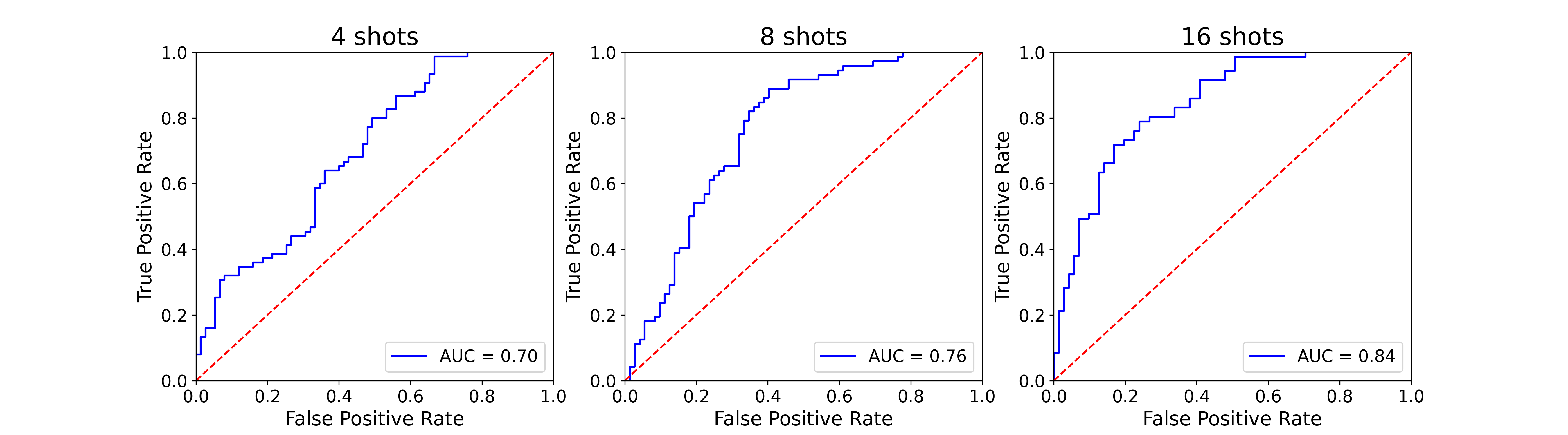
Figure 2: Results on the same/different experiments. Each column shows the results of classifying pairs of dataset with a certain number of shots.

The results of the same/different task classification experiment confirm that gradients can be used as features to capture task nature and distinguish between tasks. To further evaluate the quality of the task embeddings learned by our model, we visualize the learned task embeddings in 2D space. We find the task embeddings form good quality clusters according to task nature at higher layers. More details can be found in Appendix E.

Table 2: Ablation results.

Model	Mean Acc.
Grad2Task w/ Gradients	45.99
ProtoNet Longer Training	45.10
Grad2Task w/ X	45.66
Grad2Task w/ X&Y	45.16
Grad2Task Adapt All	44.57
Grad2Task w/ Pretrained TaskEmb	45.68
Hypernetwork	44.79

6.2 Ablation Study

We conduct ablation studies to justify our decision choices. We report the average accuracy on meta-testing datasets of different model variants in Table 2. Results show that our approach achieves the best average accuracy among all model variants, resulting in average accuracy of 45.99%. The full results are included in Appendix F.

Does the adaptation really help? Starting from the base model trained after the first stage, we compare our approach with just training the base model using the ProtoNet loss for the same number of steps. Shown as “ProtoNet Longer Training” in Table 2, the performance of this approach is worse than our proposed approach. This justifies that we can do better by adapting the base model than training it for more steps.

How are gradients compared with other task representations? We compare our approach with other CNP-based approaches with different methods of task embedding. Similar to  Requeima et al. [37], we use the average embeddings of the training sequences as representations for a task, and keep the other model architecture unchanged. We also consider using the embeddings of both input sequences and labels for task representation. We treat labels as normal text instead of discrete values and encode them using the BERT model. The label embedding and average input embeddings are concatenated as the task representation. Shown as “Grad2Task w/ X” and “Grad2Task w/ X&Y”, respectively, in Table 2, both of these two approach underperform our gradient-based method while “Grad2Task w/ X” performs closely with our method. Note that we can also combine those methods for task representation, which we leave for future work.

Adapt all or just “[CLS]"? The only difference between this model and ours is whether we apply the generated adaptation parameters only on the hidden representation of the “[CLS]" token or on all tokens in each sequence. Shown as “Grad2Task Adapt All” in Table 2, this model performs worse, resulting in 44.57% on average.

Generating model parameters or adaptation parameters? We also experimented with a hypernetwork [20]-based approach. Conditioned on the task representation, we use a neural network (hypernetwork) to output the parameters of bottleneck adapters directly, instead of freezing the bottleneck adapters and only generating scaling/shifting parameters, as in our proposed model. The model with a hypernetwork has higher flexibility for task adaptation, but the size of the hypernework is large, as it maps high-dimensional gradient information to high-dimensional model parameters, which brings challenges for optimization and suceptibility for overfitting. As shown in Table 2, it achieves accuracy of 44.79% on average and is worse than our proposed approach.

Pretraining task embedding? For this model, we first pretrain the task embedding model for the same/different tasks, then freeze and combine it with other components following our proposed approach. We observe that it has close but slightly worse performance (45.68%) than Grad2Task without task embedding pretraining. We hypothesize the task embedding trained with the same/different tasks is not good enough. We expect this model will benefit from pretraining the task embedding model on a set of datasets with higher diversity and training the task embedding model using more advanced metric-learning approaches, which we leave for future work.

7 Discussion and Conclusion

In this paper, we propose a novel model-based meta-learning approach for few-shot text classification and show the feasibility of using gradient information for task conditioning. Our approach is explicitly designed for learning from diverse text classification tasks how to adapt a base model conditioned on different tasks. We use pretrained BERT with bottleneck adapters as the base model and modulate the adapters conditioned on task representations based on gradient information.

Our work is an inaugural exploration of using gradient-based task representations for meta-learning. It has several limitations. First, the way we use neural networks to encode high-dimensional data significantly increases the number of parameters to train. For future work, we will explore more efficient ways for FIM calculation and better ways to handle high-dimensional gradient information. Second, we only focus on text sequence classification tasks in this paper. There are various types of NLP tasks to explore, such as question answering and sequence labeling tasks, which present many distinct challenges. Also, we only consider transferring between text classification tasks. As shown in Vu et al. [50], positive transfer can happen among different types of NLP tasks. Thus, we intend to explore meta-learning or transfer learning approaches to learning from different types of tasks.

Ethical Concerns.

Our work advances the field of few-shot text classification. While not having any direct negative societal impact, one can imagine that a few-shot text classifier is abused by a malicious user. For example, classifying trendy keywords on the internet naturally falls into the application area of our method as example phrases containing the new keyword can be limited in number. Toxic language is known to be a pervasive problem in the Internet [3], and a malicious user could use a good few-shot text classifier to further perpetuate these problems (e.g., by classifying toxic text as benign and fooling the end user). On the other hand, the same system can be used to promote fairness.

Appendix

Appendix A Notations

In Table A1, we list the notions that are used throughout the paper.

Table A1: List of notations.

Symbol	Description
$x$	Input features.
$y$	Output label.
$\mathcal{S}$	A support set.
$\mathcal{Q}$	A query set.
$\mathcal{S}^{c}$	The subset of examples in $S$ that belong to class $c$: $\mathcal{S}^{c}=\{(x_{i},y_{i})\,|\,(x_{i},y_{i})\in\mathcal{S},y_{i}=c\}$
$f$	The base model. We use a pretrained BERT model, insert bottleneck adapters into each transformer layer and add a linear output layer.
$\theta$	Parameters of pretrained BERT model.
$\alpha$	Parameters of the bottleneck adapters.
$\omega$	Parameters of the linear output layer.
$\Theta$	$\Theta=\{\theta,\alpha,\omega\}$.
$\mu^{c}$	The centroid of $\mathcal{S}^{c}$ which is the average embedding of the examples in $\mathcal{S}^{c}$.
$\hat{p}(x)$	The empirical distribution over $x$ specified by a dataset.
$\nabla_{\Theta}$	The gradients with regard to $\Theta$.
$F_{\Theta}$	The Fisher Information Matrix of $\Theta$.
$d$	The task embedding network.
$\phi$	Parameters of the task embedding network.
$a$	The adaptation network.
$\psi$	Parameters of the adaptation network.
$\gamma$	Scaling parameters for adaptation.
$\beta$	Shifting parameters for adaptation.

Appendix B ProtoNet Training

Algorithm 2 shows the pseudocode for training the base model during the first stage. The training procedure follows Snell et al. [41] broadly. Different with regular episodic training where episodes are sampled from a single large dataset, we have multiple meta-training datasets to sample episodes from. Accordingly, we first sample a meta-training dataset with probability proportional to the square root of its size and then sample an episode from that dataset. We repeat this process to generate episodes for meta-training. We also make sure each episode contains equal number of examples for all classes of the dataset it is sampled from.

Input :  $T$: A set of text classification tasks for training. $\mathcal{D}_{i}$: The labeled dataset of each task $i$. $\theta$: Parameters of pretrained BERT.

Output : $\alpha$: Parameters of the bottleneck layers. $\omega$: Parameters of the linear layer after BERT.

1 while not converged do

2       Sample $M$ episodes $\{t_{i}\}_{i=1}^{M}$, each episode $t_{i}=(\mathcal{S}_{i},\mathcal{Q}_{i}),\mathcal{S}_{i}\subseteq\mathcal{D}_{i},\mathcal{Q}_{i}\subseteq\mathcal{D}_{i}$

3       for $i\leftarrow 1$ to $M$ do

4             $\mu_{c}=\frac{1}{|\mathcal{S}^{c}|}\Sigma_{x_{j}\in\mathcal{S}^{c}}f(x_{j};\theta,\alpha,\omega),S^{c}=\{(x_{j},y_{j})\,|\,(x_{j},y_{j})\in\mathcal{S}_{i},y_{j}=c\}$ // build

5             // prototype of each class

6             $p(y=c|x_{j})=\mathrm{softmax}(\mathrm{euc}(f(x_{j};\theta,\alpha,\omega),\mu_{c})),(x_{j},y_{j})\in\mathcal{Q}_{i}$

7             $\ell_{i}=-\sum_{x_{j}\in\mathcal{Q}_{i}}\log p(y=y_{j}|x_{j}),(x_{j},y_{j})\in\mathcal{Q}_{i}$ // calcualte loss on the

8             // query set            

9            

10       end for

11      $\{\alpha,\omega\}\leftarrow\{\alpha,\omega\}-lr\cdot\nabla_{\{\alpha,\omega\}}\frac{1}{M}\sum_{i=1}^{M}\ell_{i}$

12 end while

Algorithm 2 Training a prototypical network with BERT and bottleneck adapters as encoder.

Appendix C Experiment Datasets

Table A2 shows the datasets we use for meta-training, which are the same with the datasets used by Bansal et al. [5] except for SST-2: Bansal et al. [5] used SST-2 as an entity typing task while we used it as a sentence-level sentiment classification task. We use the average performance on the validation sets of all meta-training tasks for hyperparameter searching and early stopping.

Table A2: Meta-training datasets.

Dataset	Task	Labels	#Training	#Validation
MRPC [16]	Paraphase	"paraphase", "not paraphase"	3668	409
QQP [22]	detection	"paraphase", "not paraphase"	363846	40430
QNLI [52]	NLI	"entailment", "not entailment"	104743	5463
RTE [14]		"entailment", "not entailment"	2490	277
SNLI [11]		"contradiction", "entailment", "neutral"	549367	9824
MNLI [53]		"contradiction", "entailment", "neutral"	392702	19647
SST-2 [42]	Movie review classification	"negative", "positive"	67349	872

Table A3 lists the datasets we use for meta-testing. We consider 4-shot, 8-shot and 16-shot for each task. For each task with a certain number of shots, we train on 10 different training sets and test on the full testing set, and report the mean and standard deviation of the testing performance over the 10 runs. We reuse most of the meta-testing datasets used by Bansal et al. [5] but remove all the datasets of which the average number of words per input sentence is larger than 100. In addition, we add three new datasets to increase the diversity of the meta-testing tasks.

Following Bansal et al. [5], we use several text classification datasets from crowdflower, including airline, disaster, emotion, political_audience, political_bias and political_message. We also use product rating dataset from the Amazon Reviews dataset [9] but only keep rating_kitchen. We add three different datasets to increase the diversity of the meta-testing tasks. We use a subset of the Yelp dataset , named yelp in Table A3. We randomly sample 2000 examples for each class as the testing set. For training, similar with other tasks, we randomly sample 10 training sets for each number of shots. SNIPS [12] is a commonly used benchmarking dataset for intent detection and slot filling tasks. We use the full test set of SNIPS and randomly sample few-shot datasets from its training set. The HuffPost dataset [27] is about classifying categories of news posted on HuffPost. The full dataset contains 41 categories, from which we randomly select 10 categories and 400 examples for each category as the testing set.

We only considered the 12 datasets in the main table of [5] and removed the two entity typing tasks, because they are phrase-level classification tasks while we only focus on sentence-level classification tasks. And we removed the other 3 tasks because they contain many sentences that exceed the max sequence length of 128. Note that we use 128 as the max length for fair comparison with [6], since it had the same restriction.

Table A3: Meta-testing datasets. Newly added datasets are marked with “*”.

Dataset	Task	#Test Size	Labels
airline	Sentiment classification on tweets about airline	7319	"neutral", "negative", "positive"
rating_kitchen	Product rating classification on Amazon	7379	"4", "2", "5"
disaster	Classifying whether tweets are relavant to disasters	5430	"not relevant", "relevant"
emotion	Emotion classification	20000	"enthusiasm", "love", "hate", "neutral", "worry", "anger", "fun", "happiness", "boredom", "sadness", "surprise", "empty", "relief"
political_audience	Classifying the audience/bias/message of social media messages from politicians	996	"national", "constituency"
political_bias		1287	"partisan", "neutral"
political_message		428	"personal", "policy", "support", "media", "attack", "other", "information", "constituency", "mobilization"
snips*	Intent detection	700	"play music", "add to playlist", "rate book", "search screening event", "book restaurant", "get weather", "search creative work"
huffpost_10*	Category classification on news headlines from HuffPost	4000	"politics", "entertainment", "travel", "wellness", etc.
yelp*	Business rating classification on Yelp	10000	"1", "2", "3", "4", "5"

Appendix D Experiment details

D.1 Comparing our Leopard implementation with [5]

We compare the results of our implementation of ProtoNet (with BERT as encoder) and Leopard with the results reported by Bansal et al. [5]. Note that here we use the same meta-testing datasets as Bansal et al. [5] without removing the datasets that contain many long sentences, namely, rating_dvd, rating_electronics and rating_books, and without adding new tasks for fair comparison. Results are shown in Table A4. The average accuracy of our Leopard implementation over all tasks is 47.59%, which is close to the average accuracy reported by Bansal et al. [5] (48.22%). However, the average accuracy of our ProtoNet implementation (51.22%) is much better than the performance reported by Bansal et al. [5] (42.36%), and is even better than Leopard. See Table A4 for detailed results on each task.

Table A4: Comparison between [5] and our implementation. “#” refers to number of shots. “Leopard ProtoNet” refers to the ProtoNet with BERT as encoder implemented by [5]. “Leopard” refers to the MAML-based approach proposed and implemented by [5]. “Our ProtoNet” refers to the ProtoNet with BERT as encoder implemented by us. “Our Leopard” refers to the Leopard model implemented by us. Note in this table, we did not remove the datasets containing very long sentences, namely, rating_dvd, rating_electronics and rating_books.

#	model	Leopard ProtoNet	Leopard	Our ProtoNet	Our Leopard
4	airline	40.27 ± 8.19	54.95 ± 11.81	65.39 ± 12.73	48.21 ± 17.99
	disaster	50.87 ± 1.12	51.45 ± 4.25	54.01 ± 2.90	51.32 ± 4.11
	emotion	9.18 ± 3.14	11.71 ± 2.16	11.69 ± 1.87	11.27 ± 3.92
	political_audience	51.47 ± 3.68	52.60 ± 3.51	52.77 ± 5.86	53.54 ± 4.15
	political_bias	56.33 ± 4.37	60.49 ± 6.66	58.26 ± 10.42	58.08 ± 9.19
	political_message	14.22 ± 1.25	15.69 ± 1.57	17.82 ± 1.33	16.82 ± 1.79
	rating_books	48.44 ± 7.43	54.92 ± 6.18	60.12 ± 8.05	56.94 ± 10.43
	rating_dvd	47.73 ± 6.20	49.76 ± 9.80	56.95 ± 10.17	44.68 ± 11.29
	rating_electronics	37.40 ± 3.72	51.71 ± 7.20	57.32 ± 7.61	51.61 ± 8.83
	rating_kitchen	44.72 ± 9.13	50.21 ± 9.63	58.47 ± 11.12	48.77 ± 12.44
	Average	40.06 ± 4.82	45.35 ± 6.28	49.28 ± 7.21	44.12 ± 8.41
8	airline	51.16 ± 7.60	61.44 ± 3.90	69.14 ± 4.84	65.68 ± 11.79
	disaster	51.30 ± 2.30	55.96 ± 3.58	54.48 ± 3.17	50.37 ± 3.31
	emotion	11.18 ± 2.95	12.90 ± 1.63	13.10 ± 2.64	13.03 ± 5.99
	political_audience	51.83 ± 3.77	54.31 ± 3.95	55.17 ± 4.28	52.15 ± 5.57
	political_bias	58.87 ± 3.79	61.74 ± 6.73	63.22 ± 1.96	62.69 ± 1.08
	political_message	15.67 ± 1.96	18.02 ± 2.32	20.40 ± 1.12	17.38 ± 1.92
	rating_books	52.13 ± 4.79	59.16 ± 4.13	62.59 ± 8.11	63.13 ± 8.08
	rating_dvd	47.11 ± 4.00	53.28 ± 4.66	59.18 ± 7.00	53.42 ± 9.54
	rating_electronics	43.64 ± 7.31	54.78 ± 6.48	61.57 ± 2.94	58.43 ± 3.08
	rating_kitchen	46.03 ± 8.57	53.72 ± 10.31	57.08 ± 11.54	53.19 ± 12.05
	Average	42.89 ± 4.70	48.53 ± 4.77	51.59 ± 4.76	48.95 ± 6.24
16	airline	48.73 ± 6.79	62.15 ± 5.56	71.06 ± 1.60	67.04 ± 8.06
	disaster	52.76 ± 2.92	61.32 ± 2.83	55.30 ± 2.68	50.37 ± 4.27
	emotion	12.32 ± 3.73	13.38 ± 2.20	12.81 ± 1.21	10.30 ± 2.86
	political_audience	53.53 ± 3.25	57.71 ± 3.52	56.16 ± 2.81	54.94 ± 2.34
	political_bias	57.01 ± 4.44	65.08 ± 2.14	61.98 ± 6.89	61.38 ± 5.03
	political_message	16.49 ± 1.96	18.07 ± 2.41	21.36 ± 0.86	18.22 ± 1.88
	rating_books	57.28 ± 4.57	61.02 ± 4.19	65.82 ± 4.65	63.98 ± 9.32
	rating_dvd	48.39 ± 3.74	53.52 ± 4.77	61.86 ± 1.89	55.27 ± 8.91
	rating_electronics	44.83 ± 5.96	58.69 ± 2.41	60.49 ± 4.86	58.05 ± 3.49
	rating_kitchen	49.85 ± 9.31	57.00 ± 8.69	61.00 ± 9.17	57.34 ± 10.82
	Average	44.12 ± 4.67	50.79 ± 3.87	52.78 ± 3.66	49.69 ± 5.70

D.2 Implementation details

Our codes are publicly available on https://github.com/jixuan-wang/Grad2Task. During meta-training, after sampling episodes with roughly the same number of examples as the total number of examples in the meta-training datasets, we refer this as one epoch. For all models, we train them on the meta-training datasets for 5 epochs and report results of the models with the best average performance on the validation sets of all meta-training tasks. To calculate the ProtoNet loss, we tried both Euclidean distance and cosine distance as the distance metric, and found that Euclidean distance worked better and so used it for all experiments. The linear layer on top of BERT has the size of 256. The task embedding network is a 2 layers GRU model, of which the input size is 24567 (i.e., the parameter size in each bottleneck adapter) and the output size is task embedding size (we used 100). The adaptation networks are single layer MLPs.

We use dropout rate [44] of 0.1 for all models. We choose learning rate for each model from $\{1e-5,2e-5,5e-5,1e-4\}$ based on the validation performance. We use the Adam algorithm [24] for optimization. We perform one optimization step after seeing 4 episodes. Note that our approach does not require tuning any hyperparameters like the number of steps in inner loop as in MAML based approches [5]. Each model is trained on 2 NVIDIA Tesla P100 GPUs.

Parameter size of the BERT_BASE model is  110M but all of its parameters are kept fixed in our method. We insert 24 bottleneck adapters into the BERT_BASE model, which consume  7M parameters in total and are only trained in the first stage. The task embedding network contains  7M parameters. The adaptation network contains  1.3M parameters for each bottleneck adapter.

Training PN-BERT and PN-BN took  9 and  7 hours, respectively, on two Tesla P100 GPUs. In the second stage of our method, the task embedding network and adaptation network are trained together for 5 epochs on the meta-training datasets, which took  4 hours on two Tesla P100 GPUs.

Appendix E Visualization of task embeddings

We visualize the task embeddings learned by the task embedding network in Figure A1. We show the per-layer task embeddings of the meta-training tasks after being mapped into the 2D space by t-SNE [48]. Each point in Figure A1 is corresponding to an episode or task sampled from a meta-training dataset. For each episode, we first calculate the raw gradient information and then feed it into the RNN-based task embedding network, which outputs the per-layer task embeddings. Note that for the 12-layer BERT_BASE model we inserted two adapters into each transformer layer, so there are 24 task embeddings in total for each episode. Here we only visualize the first task embedding at each transformer layer, resulting in 12 task embeddings for each episode. From Figure A1 we observe that the task embeddings form better clusters at higher layers. At the last layer, the only movie review classification task (SST-2) is separated clearly from other tasks, multiple NLI tasks are mixed together in the top center, and the paraphrase detection tasks QQP and MRPC spread in the center.

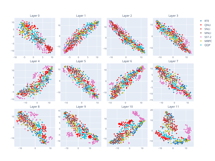
Figure A1: T-SNE visualization of the learned task embeddings. Each sub-figure is the task embeddings at a certain layer, e.g., “Layer 11” refers to the task embeddings at the last transformer layer of BERT_BASE. Each point is an episode or task sampled from a dataset. Each color is corresponding to a dataset.

Appendix F Ablation results details

Details of the ablation study results are shown in Table A5. First, all variants under our framework achieve better performance than previous work [5] and other baselines, i.e., ProtoNet [41]-based and Hypernet [20]-based approaches. Second, overall, the model with gradients as task representation (shown as “Grad2Task w/ Gradients”) performs the best: for the ten meta-testing tasks being considered, it achieves the best performance among all the variants for five 4-shot tasks, four 8-shot tasks and four 16-shot tasks.

Table A5: Detailed results of the ablation study. “#” refers to number of shots. We show both the mean and standard deviation of the accuracy over 10 runs. For example, in “66.78 ± 6.27”, “66.78” refers to the average accuracy and “6.27” refers to the standard deviation of accuracy. We further average the results of each model for each number of shots, shown as the rows in grey color. All models shown in this table are trained by starting from the same base model after the first training stage. “PN Longer Training” refers to training the base model for more iterations without any adaptation. “Grad2Task X” is similar with our proposed model but uses average input encoding as task representation. “Grad2Task X&Y” is similar with our proposed model but uses average input encoding and textual label encoding as task representation. “Grad2Task Adapt All” refers to our proposed model but adapting the hidden representation of all input tokens instead of just the “[CLS]” token. “Grad2Task w/ Pretrained Emb” refers to our proposed model but using task embedding model pretrained on the same/different task. “Hypernet” is similar with our proposed approach but generating whole parameters for the bottleneck adapters instead of adaptation parameters. “Grad2Task w/ Gradients” refers to our proposed approach.

	Model:	PN Longer	Grad2Task X	Grad2Task	Grad2Task	Grad2Task w/	Hypernet	Grad2Task w/
#		Training		X&Y	Adapt All	Pretrained Emb		Gradients
4	airline	66.78 ± 6.27	66.58 ± 11.92	66.88 ± 11.55	66.83 ± 12.17	67.76 ± 10.48	62.99 ± 7.54	70.64 ± 3.95
	disaster	53.46 ± 3.64	54.97 ± 6.83	53.54 ± 4.34	54.22 ± 5.93	54.83 ± 6.19	54.84 ± 5.69	55.43 ± 5.89
	emotion	12.64 ± 1.98	13.27 ± 1.90	12.80 ± 1.60	13.21 ± 2.27	12.80 ± 1.64	13.16 ± 1.17	12.76 ± 1.35
	political_audience	52.78 ± 5.57	52.79 ± 6.99	51.32 ± 6.15	53.01 ± 7.00	52.27 ± 6.15	50.59 ± 4.80	51.28 ± 5.74
	political_bias	63.52 ± 1.94	62.24 ± 6.50	59.63 ± 7.79	61.51 ± 7.07	60.30 ± 7.04	60.35 ± 6.72	58.74 ± 9.43
	political_message	20.69 ± 1.26	20.87 ± 1.36	20.22 ± 1.81	19.69 ± 1.53	20.31 ± 1.65	17.18 ± 1.77	21.13 ± 1.97
	rating_kitchen	55.29 ± 10.29	56.27 ± 9.19	57.22 ± 10.25	56.69 ± 10.75	56.88 ± 9.71	56.78 ± 8.12	57.09 ± 9.74
	huffpost_10	17.59 ± 2.69	17.01 ± 1.80	17.14 ± 1.77	16.94 ± 1.88	17.67 ± 2.27	17.00 ± 2.63	18.50 ± 2.00
	snips	47.77 ± 4.08	50.16 ± 2.89	47.46 ± 3.88	43.36 ± 2.39	49.09 ± 4.11	49.76 ± 4.67	52.51 ± 2.68
	yelp	41.68 ± 3.07	43.04 ± 2.63	41.65 ± 2.90	42.45 ± 3.25	42.50 ± 3.48	42.20 ± 3.15	43.00 ± 3.55
	Average	43.22 ± 4.08	43.72 ± 5.20	42.79 ± 5.20	42.79 ± 5.42	43.44 ± 5.27	42.48 ± 4.63	44.11 ± 4.63
8	airline	70.27 ± 2.11	71.86 ± 3.52	71.67 ± 3.31	71.49 ± 2.23	72.51 ± 2.25	68.44 ± 2.59	72.04 ± 2.58
	disaster	54.75 ± 3.88	56.71 ± 6.55	56.59 ± 3.14	55.86 ± 3.99	55.34 ± 3.40	55.79 ± 4.16	57.49 ± 5.36
	emotion	13.62 ± 1.79	14.14 ± 2.20	13.92 ± 1.60	14.15 ± 2.38	14.46 ± 2.08	14.33 ± 1.44	13.99 ± 1.90
	political_audience	53.46 ± 5.05	53.65 ± 6.44	53.55 ± 6.19	54.56 ± 5.62	52.97 ± 5.79	52.39 ± 4.69	52.60 ± 5.55
	political_bias	64.69 ± 0.73	65.07 ± 0.76	64.25 ± 0.96	64.32 ± 0.44	64.90 ± 1.12	63.68 ± 1.43	64.06 ± 1.12
	political_message	21.76 ± 0.89	21.71 ± 1.77	21.13 ± 1.81	21.29 ± 1.03	21.04 ± 1.76	20.18 ± 2.05	21.31 ± 1.16
	rating_kitchen	56.68 ± 10.99	57.50 ± 10.17	58.11 ± 9.77	56.62 ± 10.61	57.72 ± 10.41	55.46 ± 10.99	58.35 ± 9.83
	huffpost_10	19.81 ± 2.53	19.97 ± 1.47	20.31 ± 1.74	19.07 ± 1.75	20.97 ± 1.54	18.93 ± 1.62	21.12 ± 1.69
	snips	54.27 ± 3.11	53.81 ± 2.63	52.56 ± 2.23	48.49 ± 4.41	53.83 ± 2.30	56.41 ± 3.47	57.19 ± 2.77
	yelp	43.26 ± 1.85	45.15 ± 1.61	44.20 ± 1.69	43.73 ± 1.73	44.26 ± 1.98	42.90 ± 3.19	43.66 ± 1.65
	Average	45.26 ± 3.29	45.96 ± 3.71	45.63 ± 3.24	44.96 ± 3.42	45.80 ± 3.26	44.85 ± 3.56	46.18 ± 3.36
16	airline	70.20 ± 1.62	72.25 ± 1.94	72.09 ± 1.93	71.64 ± 1.63	72.79 ± 1.58	67.87 ± 1.62	72.30 ± 1.75
	disaster	57.05 ± 4.46	57.46 ± 2.47	58.45 ± 2.92	56.73 ± 3.37	58.83 ± 5.32	58.94 ± 3.56	59.63 ± 3.11
	emotion	14.28 ± 1.46	14.02 ± 0.93	14.04 ± 1.29	13.91 ± 0.78	14.23 ± 1.32	14.54 ± 0.90	13.72 ± 1.24
	political_audience	56.86 ± 3.01	57.79 ± 4.02	56.71 ± 3.62	56.98 ± 4.15	56.99 ± 2.44	55.79 ± 2.72	55.46 ± 3.34
	political_bias	64.67 ± 0.72	65.36 ± 0.77	64.06 ± 0.53	64.21 ± 0.18	64.29 ± 2.88	64.33 ± 0.60	63.83 ± 0.74
	political_message	23.44 ± 0.91	23.64 ± 1.26	23.00 ± 1.19	22.31 ± 1.23	23.89 ± 1.11	22.29 ± 2.32	22.22 ± 1.20
	rating_kitchen	59.64 ± 9.14	61.03 ± 6.64	60.72 ± 6.38	59.35 ± 8.78	61.68 ± 6.81	59.48 ± 7.01	61.72 ± 6.38
	huffpost_10	21.96 ± 1.30	21.45 ± 1.87	21.98 ± 1.78	20.48 ± 1.73	22.56 ± 1.27	21.34 ± 2.19	23.57 ± 1.76
	snips	56.21 ± 2.40	55.65 ± 1.55	55.16 ± 2.37	49.89 ± 2.96	57.19 ± 2.08	61.81 ± 1.45	59.47 ± 1.91
	yelp	43.80 ± 2.17	44.43 ± 2.90	44.53 ± 2.23	44.25 ± 2.25	45.39 ± 1.35	43.85 ± 2.14	44.87 ± 2.09
	Average	46.81 ± 2.72	47.31 ± 2.44	47.07 ± 2.42	45.97 ± 2.71	47.78 ± 2.62	47.02 ± 2.45	47.68 ± 2.35

Appendix G Additional results

G.1 Results on all datasets

We did not report results on the datasets used by [5] for domain adaptation and ablations, since we focus on evaluation generalization to tasks with different structure. However, we did run evaluation on all datasets of [5] (except entity typing datasets since they are phrase-level classification tasks). Table LABEL:tb:all_datasets shows the average accuracy under each shot, demonstrating that our conclusion holds.

Table A6: Average accuracy on all datasets used by Bansal et al. [5]. “*”: results reported by [5].

Model	K4	K8	K16
Leopard*	52.61	56.02	57.97
PN-BN	56.5	57.94	59.69
Grad2Task	57.05	58.37	59.7

G.2 Comparison with other fine-tuning baselines

The main disadvantage of fine-tuning approaches is that they require costly retraining on new tasks and hand tuning and are more vulnerable to overfitting on few-shot problems. To illustrate this we compare different fine-tuning approaches in the table below (FT: fine-tuning, BN: bottleneck adapters, PN: ProtoNet, *: numbers reported in [5]). We show the average accuracy on a subset of tasks from [5] with 4, 8 and 16 shots. For example, FT-PN-BN refers to only fine-tuning the BN parameters of a trained ProtoNet. Results show all fine-tuning approaches perform much worse on 4-shot problems than our method, while some of them start to catch up with more shots, i.e., 16-shot.

Table A7: Comparison with other fine-tuning approaches. “*”: results reported in [5].

model	K4	K8	K16
FT-BERT*	37.79	37.05	46.28
FT-BERT-BN	37.29	36.96	37.92
FT-PT-BN-FILM	40.95	45.83	49.74
FT-PT-BN	41.68	46.33	49.27
FT-PT	41.52	47.24	49.85
FT-BERT	38.5	39.4	45.21
PN	45.49	47.51	48.52
PN-BN	45.98	47.64	49.63
Grad2Task	46.72	48.55	49.84

References

- [1] Yelp open dataset. https://www.yelp.com/dataset. (Accessed on 05/20/2021).
- Achille et al. [2019] A. Achille, M. Lam, R. Tewari, A. Ravichandran, S. Maji, C. C. Fowlkes, S. Soatto, and P. Perona. Task2vec: Task embedding for meta-learning. In Proceedings of the IEEE/CVF International Conference on Computer Vision, pages 6430–6439, 2019.
- Adragna et al. [2020] R. Adragna, E. Creager, D. Madras, and R. Zemel. Fairness and robustness in invariant learning: A case study in toxicity classification. arXiv preprint arXiv:2011.06485, 2020.
- Baik et al. [2020] S. Baik, S. Hong, and K. M. Lee. Learning to forget for meta-learning. In Proceedings of the IEEE/CVF Conference on Computer Vision and Pattern Recognition, pages 2379–2387, 2020.
- Bansal et al. [2020a] T. Bansal, R. Jha, and A. McCallum. Learning to few-shot learn across diverse natural language classification tasks. In Proceedings of the 28th International Conference on Computational Linguistics, pages 5108–5123, 2020a.
- Bansal et al. [2020b] T. Bansal, R. Jha, T. Munkhdalai, and A. McCallum. Self-supervised meta-learning for few-shot natural language classification tasks. In Proceedings of the 2020 Conference on Empirical Methods in Natural Language Processing (EMNLP), pages 522–534, 2020b.
- Bao et al. [2019] Y. Bao, M. Wu, S. Chang, and R. Barzilay. Few-shot text classification with distributional signatures. In International Conference on Learning Representations, 2019.
- Bingel and Søgaard [2017] J. Bingel and A. Søgaard. Identifying beneficial task relations for multi-task learning in deep neural networks. In Proceedings of the 15th Conference of the European Chapter of the Association for Computational Linguistics: Volume 2, Short Papers, pages 164–169, 2017.
- Blitzer et al. [2007] J. Blitzer, M. Dredze, and F. Pereira. Biographies, Bollywood, boom-boxes and blenders: Domain adaptation for sentiment classification. In Proceedings of the 45th Annual Meeting of the Association of Computational Linguistics, pages 440–447, Prague, Czech Republic, June 2007. Association for Computational Linguistics. URL https://www.aclweb.org/anthology/P07-1056.
- Bowman et al. [2015a] S. R. Bowman, G. Angeli, C. Potts, and C. D. Manning. A large annotated corpus for learning natural language inference. In Proceedings of the 2015 Conference on Empirical Methods in Natural Language Processing, pages 632––642, 2015a.
- Bowman et al. [2015b] S. R. Bowman, G. Angeli, C. Potts, and C. D. Manning. A large annotated corpus for learning natural language inference. In Proceedings of the 2015 Conference on Empirical Methods in Natural Language Processing, pages 632–642, Lisbon, Portugal, Sept. 2015b. Association for Computational Linguistics. doi: 10.18653/v1/D15-1075. URL https://www.aclweb.org/anthology/D15-1075.
- Coucke et al. [2018a] A. Coucke, A. Saade, A. Ball, T. Bluche, A. Caulier, D. Leroy, C. Doumouro, T. Gisselbrecht, F. Caltagirone, T. Lavril, M. Primet, and J. Dureau. Snips voice platform: an embedded spoken language understanding system for private-by-design voice interfaces. CoRR, abs/1805.10190, 2018a. URL http://arxiv.org/abs/1805.10190.
- Coucke et al. [2018b] A. Coucke, A. Saade, A. Ball, T. Bluche, A. Caulier, D. Leroy, C. Doumouro, T. Gisselbrecht, F. Caltagirone, T. Lavril, et al. Snips voice platform: an embedded spoken language understanding system for private-by-design voice interfaces. arXiv preprint arXiv:1805.10190, 2018b.
- Dagan et al. [2005] I. Dagan, O. Glickman, and B. Magnini. The pascal recognising textual entailment challenge. In Machine Learning Challenges Workshop, pages 177–190. Springer, 2005.
- Devlin et al. [2019] J. Devlin, M.-W. Chang, K. Lee, and K. Toutanova. BERT: Pre-training of deep bidirectional transformers for language understanding. In Proceedings of the 2019 Conference of the North American Chapter of the Association for Computational Linguistics: Human Language Technologies, Volume 1 (Long and Short Papers), pages 4171–4186, 2019.
- Dolan and Brockett [2005] W. B. Dolan and C. Brockett. Automatically constructing a corpus of sentential paraphrases. In Proceedings of the Third International Workshop on Paraphrasing (IWP2005), 2005.
- Finn et al. [2017] C. Finn, P. Abbeel, and S. Levine. Model-agnostic meta-learning for fast adaptation of deep networks. In International Conference on Machine Learning, pages 1126–1135. PMLR, 2017.
- Garnelo et al. [2018] M. Garnelo, D. Rosenbaum, C. Maddison, T. Ramalho, D. Saxton, M. Shanahan, Y. W. Teh, D. Rezende, and S. A. Eslami. Conditional neural processes. In International Conference on Machine Learning, pages 1704–1713. PMLR, 2018.
- Geng et al. [2019] R. Geng, B. Li, Y. Li, X. Zhu, P. Jian, and J. Sun. Induction networks for few-shot text classification. In Proceedings of the 2019 Conference on Empirical Methods in Natural Language Processing and the 9th International Joint Conference on Natural Language Processing (EMNLP-IJCNLP), pages 3895–3904, 2019.
- Ha et al. [2016] D. Ha, A. Dai, and Q. V. Le. Hypernetworks. arXiv preprint arXiv:1609.09106, 2016.
- Houlsby et al. [2019] N. Houlsby, A. Giurgiu, S. Jastrzebski, B. Morrone, Q. De Laroussilhe, A. Gesmundo, M. Attariyan, and S. Gelly. Parameter-efficient transfer learning for NLP. In International Conference on Machine Learning, pages 2790–2799. PMLR, 2019.
- Iyer et al. [2017] S. Iyer, N. Dandekar, and K. Csernai. First quora dataset release: Question pairs. 2017.
- Kerineć et al. [2018] E. Kerineć, A. Søgaard, and C. Braud. When does deep multi-task learning work for loosely related document classification tasks? In Proceedings of the 2018 EMNLP Workshop BlackboxNLP: Analyzing and Interpreting Neural Networks for NLP, pages 1–8. Association for Computational Linguistics, 2018.
- Kingma and Ba [2015] D. P. Kingma and J. Ba. Adam: A method for stochastic optimization. In ICLR, 2015.
- Liu et al. [2019] Y. Liu, M. Ott, N. Goyal, J. Du, M. Joshi, D. Chen, O. Levy, M. Lewis, L. Zettlemoyer, and V. Stoyanov. RoBERTa: A robustly optimized BERT pretraining approach. arXiv preprint arXiv:1907.11692, 2019.
- [26] R. Misra. News category dataset. https://www.kaggle.com/rmisra/news-category-dataset. (Accessed on 05/20/2021).
- Misra [2018] R. Misra. News category dataset. 2018.
- Munkhdalai and Yu [2017] T. Munkhdalai and H. Yu. Meta networks. In International Conference on Machine Learning, pages 2554–2563. PMLR, 2017.
- Nguyen et al. [2020] C. Nguyen, T. Hassner, M. Seeger, and C. Archambeau. Leep: A new measure to evaluate transferability of learned representations. In International Conference on Machine Learning, pages 7294–7305. PMLR, 2020.
- Nichol et al. [2018] A. Nichol, J. Achiam, and J. Schulman. On first-order meta-learning algorithms. arXiv preprint arXiv:1803.02999, 2018.
- Oreshkin et al. [2018] B. N. Oreshkin, P. Rodriguez, and A. Lacoste. TADAM: task dependent adaptive metric for improved few-shot learning. In Proceedings of the 32nd International Conference on Neural Information Processing Systems, pages 719–729, 2018.
- Perez et al. [2018] E. Perez, F. Strub, H. De Vries, V. Dumoulin, and A. Courville. Film: Visual reasoning with a general conditioning layer. In Proceedings of the AAAI Conference on Artificial Intelligence, volume 32, 2018.
- Phang et al. [2018] J. Phang, T. Févry, and S. R. Bowman. Sentence encoders on stilts: Supplementary training on intermediate labeled-data tasks. arXiv preprint arXiv:1811.01088, 2018.
- Radford et al. [2018] A. Radford, K. Narasimhan, T. Salimans, and I. Sutskever. Improving language understanding by generative pre-training. 2018.
- Raffel et al. [2020] C. Raffel, N. Shazeer, A. Roberts, K. Lee, S. Narang, M. Matena, Y. Zhou, W. Li, and P. J. Liu. Exploring the limits of transfer learning with a unified text-to-text transformer. Journal of Machine Learning Research, 21:1–67, 2020.
- Ravi and Larochelle [2016] S. Ravi and H. Larochelle. Optimization as a model for few-shot learning. 2016.
- [37] J. Requeima, J. Gordon, J. Bronskill, S. Nowozin, and R. Turner. Fast and flexible multi-task classification using conditional neural adaptive processes. Advances in Neural Information Processing Systems 32 (NIPS 2019).
- Rusu et al. [2018] A. A. Rusu, D. Rao, J. Sygnowski, O. Vinyals, R. Pascanu, S. Osindero, and R. Hadsell. Meta-learning with latent embedding optimization. In International Conference on Learning Representations, 2018.
- Santoro et al. [2016] A. Santoro, S. Bartunov, M. Botvinick, D. Wierstra, and T. Lillicrap. Meta-learning with memory-augmented neural networks. In International conference on machine learning, pages 1842–1850. PMLR, 2016.
- Schick and Schütze [2020] T. Schick and H. Schütze. Exploiting cloze questions for few-shot text classification and natural language inference. arXiv preprint arXiv:2001.07676, 2020.
- Snell et al. [2017] J. Snell, K. Swersky, and R. Zemel. Prototypical networks for few-shot learning. In Proceedings of the 31st International Conference on Neural Information Processing Systems, pages 4080–4090, 2017.
- Socher et al. [2013] R. Socher, A. Perelygin, J. Wu, J. Chuang, C. D. Manning, A. Ng, and C. Potts. Recursive deep models for semantic compositionality over a sentiment treebank. In Proceedings of the 2013 Conference on Empirical Methods in Natural Language Processing, pages 1631–1642, Seattle, Washington, USA, Oct. 2013. Association for Computational Linguistics. URL https://www.aclweb.org/anthology/D13-1170.
- Song et al. [2020] J. Song, Y. Chen, J. Ye, X. Wang, C. Shen, F. Mao, and M. Song. Depara: Deep attribution graph for deep knowledge transferability. In Proceedings of the IEEE/CVF Conference on Computer Vision and Pattern Recognition, pages 3922–3930, 2020.
- Srivastava et al. [2014] N. Srivastava, G. Hinton, A. Krizhevsky, I. Sutskever, and R. Salakhutdinov. Dropout: A simple way to prevent neural networks from overfitting. Journal of Machine Learning Research, 15(56):1929–1958, 2014. URL http://jmlr.org/papers/v15/srivastava14a.html.
- Sung et al. [2018] F. Sung, Y. Yang, L. Zhang, T. Xiang, P. H. Torr, and T. M. Hospedales. Learning to compare: Relation network for few-shot learning. In Proceedings of the IEEE conference on computer vision and pattern recognition, pages 1199–1208, 2018.
- Talmor and Berant [2019] A. Talmor and J. Berant. MultiQA: An empirical investigation of generalization and transfer in reading comprehension. arXiv preprint arXiv:1905.13453, 2019.
- Tran et al. [2019] A. T. Tran, C. V. Nguyen, and T. Hassner. Transferability and hardness of supervised classification tasks. In Proceedings of the IEEE/CVF International Conference on Computer Vision, pages 1395–1405, 2019.
- Van der Maaten and Hinton [2008] L. Van der Maaten and G. Hinton. Visualizing data using t-sne. Journal of machine learning research, 9(11), 2008.
- Vinyals et al. [2016] O. Vinyals, C. Blundell, T. Lillicrap, K. Kavukcuoglu, and D. Wierstra. Matching networks for one shot learning. In Proceedings of the 30th International Conference on Neural Information Processing Systems, pages 3637–3645, 2016.
- Vu et al. [2020] T. Vu, T. Wang, T. Munkhdalai, A. Sordoni, A. Trischler, A. Mattarella-Micke, S. Maji, and M. Iyyer. Exploring and predicting transferability across nlp tasks. arXiv preprint arXiv:2005.00770, 2020.
- Wang et al. [2018a] A. Wang, J. Hula, P. Xia, R. Pappagari, R. T. McCoy, R. Patel, N. Kim, I. Tenney, Y. Huang, K. Yu, et al. Can you tell me how to get past Sesame Street? Sentence-level pretraining beyond language modeling. arXiv preprint arXiv:1812.10860, 2018a.
- Wang et al. [2018b] A. Wang, A. Singh, J. Michael, F. Hill, O. Levy, and S. R. Bowman. GLUE: A multi-task benchmark and analysis platform for natural language understanding. arXiv preprint arXiv:1804.07461, 2018b.
- Williams et al. [2018] A. Williams, N. Nangia, and S. Bowman. A broad-coverage challenge corpus for sentence understanding through inference. In Proceedings of the 2018 Conference of the North American Chapter of the Association for Computational Linguistics: Human Language Technologies, Volume 1 (Long Papers), pages 1112–1122, New Orleans, Louisiana, June 2018. Association for Computational Linguistics. doi: 10.18653/v1/N18-1101. URL https://www.aclweb.org/anthology/N18-1101.
- Yogatama et al. [2019] D. Yogatama, C. d. M. d’Autume, J. Connor, T. Kocisky, M. Chrzanowski, L. Kong, A. Lazaridou, W. Ling, L. Yu, C. Dyer, et al. Learning and evaluating general linguistic intelligence. arXiv preprint arXiv:1901.11373, 2019.
- Yu et al. [2018] M. Yu, X. Guo, J. Yi, S. Chang, S. Potdar, Y. Cheng, G. Tesauro, H. Wang, and B. Zhou. Diverse few-shot text classification with multiple metrics. In Proceedings of the 2018 Conference of the North American Chapter of the Association for Computational Linguistics: Human Language Technologies, Volume 1 (Long Papers), pages 1206–1215, 2018.
- Zamir et al. [2018] A. R. Zamir, A. Sax, W. Shen, L. J. Guibas, J. Malik, and S. Savarese. Taskonomy: Disentangling task transfer learning. In Proceedings of the IEEE conference on computer vision and pattern recognition, pages 3712–3722, 2018.