Human Interpretation of Saliency-based Explanation Over Text

Abstract.

While a lot of research in explainable AI focuses on producing effective explanations, less work is devoted to the question of how people understand and interpret the explanation. In this work, we focus on this question through a study of saliency-based explanations over textual data. Feature-attribution explanations of text models aim to communicate which parts of the input text were more influential than others towards the model decision. Many current explanation methods, such as gradient-based or Shapley value-based methods, provide measures of importance which are well-understood mathematically. But how does a person receiving the explanation (the explainee) comprehend it? And does their understanding match what the explanation attempted to communicate? We empirically investigate the effect of various factors of the input, the feature-attribution explanation, and visualization procedure, on laypeople’s interpretation of the explanation. We query crowdworkers for their interpretation on tasks in English and German, and fit a GAMM model to their responses considering the factors of interest. We find that people often mis-interpret the explanations: superficial and unrelated factors, such as word length, influence the explainees’ importance assignment despite the explanation communicating importance directly. We then show that some of this distortion can be attenuated: we propose a method to adjust saliencies based on model estimates of over- and under-perception, and explore bar charts as an alternative to heatmap saliency visualization. We find that both approaches can attenuate the distorting effect of specific factors, leading to better-calibrated understanding of the explanation.

1. Introduction

Machine learning models’ application in various domains (e.g., criminal justice and healthcare) has motivated the development of explanation methods to understand their behavior. One popular class of explanation methods explains model decisions by specifying the parts of the input which are most salient in the model’s decision process (Burkart and Huber, 2021; Tjoa and Guan, 2021; Fel et al., 2021b). In natural language processing (NLP), this refers to which words, phrases or sentences in the input contributed most to the model prediction (Madsen et al., 2021b; Danilevsky et al., 2020). While much research exists on developing and verifying such explanations (Arras et al., 2017; Adebayo et al., 2018; Kindermans et al., 2019; Tuckey et al., 2019; Wang et al., 2020; Madsen et al., 2021a), less is known about the information that human explainees actually understand from them (Miller, 2019; Dinu et al., 2020; Fel et al., 2021a; Arora et al., 2021).

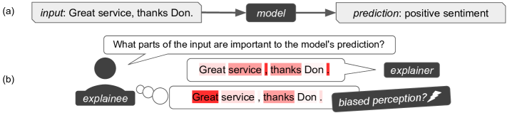
Figure 1. A saliency explantion is generated to answer the human’s need to understand the model. We investigate whether the saliency explanation can be systematically mis-perceived by humans and which factors influence its perception.

In the explainable NLP literature, it is generally (implicitly) assumed that the explainee interprets the information “correctly”, as it is communicated (Arras et al., 2017; Feng and Boyd-Graber, 2019; Fel et al., 2021a): e.g., when one word is explained to be influential in the model’s decision process, or more influential than another word, it is assumed that the explainee understands this relationship (Jacovi and Goldberg, 2021). We question this assumption: research in the social sciences describes modes in which the human explainee may be biased—via some cognitive habit—in their interpretation of processes (Malle, 2003; Miller, 2019; Epley et al., 2007; Watson, 2020). Additional research shows this effect manifests in practice in AI settings (Gonzalez et al., 2021; Darling, 2015; Ehsan et al., 2021; Hartzog, 2015; Natarajan and Gombolay, 2020). This means, for example, that the explainee may underestimate the influence of a punctuation token, even if the explanation reports that this token is highly significant (Figure 1), because the explainee is attempting to understand how the model reasons by analogy to the explainee’s own mind which is an instance of anthropomorphic bias (Johnson, 2018; Dacey, 2017; Zlotowski et al., 2015) and belief bias (Evans et al., 1983; Gonzalez et al., 2021).

We identify three different such biases which may influence the explainee’s interpretation: (i) anthropomorphic bias and belief bias: influence by the explainee’s self projection onto the model; (ii) visual perception bias: influence by the explainee’s visual affordances for comprehending information; (iii) learning effects: observable temporal changes in the explainee’s interpretation as a result of interacting with the explanation over multiple instances.

We thus address the following question in this paper: When a human explainee observes feature-attribution explanations, does their comprehended information differ from what the explanation “objectively” attempts to communicate? If so, how?

We propose a methodology to investigate whether explainees exhibit biases when interpreting feature-attribution explanations in NLP, which effectively distort the objective attribution into a subjective interpretation of it (Section 4). We conduct user studies in which we show an input sentence and a feature-attribution explanation (i.e., saliency map) to explainees, ask them to report their subjective interpretation, and analyze their responses for statistical significance across multiple factors, such as word length, total input length, or dependency relation, using GAMMs (Section 5).

We find that word length, sentence length, the position of the sentence in the temporal course of the experiment, the saliency rank, capitalization, dependency relation, word position, word frequency as well as sentiment can significantly affect user perception. In addition to whether a factor has a significant influence, we also investigate how this factor affects perception. We find that, for example, short words overall decrease importance ratings while short sentences or intense sentiment polarities increase them.

Finally, we propose two visualization interventions to mitigate learning effect and visual perception biases: model-based color correction and bar charts. We conclude that (a) model-based color correction can predict and mitigate distorting temporal effects and (b) bar charts can successfully remove the influence of word length.

Overall, our results show that supposedly irrelevant factors such as word length do affect how explainees perceive the influence of words in feature-attribution explanations, despite the explanations explicitly communicating this influence. This is a surprising result, which raises important questions for explainability in NLP, and in general, about the ability of feature-attribution tools available today to convey the information that they intend to communicate: even in the case of a relatively straightforward explanation, such as directly informing importance regions in the input, cognitive biases of explainees run deep, and may erroneously affect the understanding of the given information.

We show that bar charts and color correction result in better-aligned human assessments in our setting on multiple bias factors. We urge researchers to not blindly trust that users perceive explanations as communicated, and to investigate if our findings transfer to their respective audience and context.

2. Feature-Attribution Explanations

Feature-attribution explanations aim to convey which parts of the input to a model decision are “important”, “responsible” or “influential” to the decision (Arras et al., 2017; Ribeiro et al., 2016; Carvalho et al., 2019; Madsen et al., 2021b; Zhang et al., 2021). This class of methods is a prevalent mode of describing NLP processes (Madsen et al., 2021b; Danilevsky et al., 2020; Kaur et al., 2020; Tenney et al., 2020), due to two main strengths: (1) it is flexible and convenient, with many different measures developed to communicate some aspect of feature importance; (2) it is intuitive, with—seemingly, as we discover—straightforward interfaces of relaying this information. Here we cover background on feature-attribution on two fronts: the underlying technologies (Section 2.1) and the information which they communicate to humans (Section 2.2).

2.1. Attribution Methods

We consider feature-attribution explanations generally as scoring (or ranking) functions that map portions of the input to scores that communicate some aspect of importance about the aligned portion: $E_{f}(f(\mathbf{x})):\Sigma^{n}\rightarrow\mathbb{R}^{n},$ where $E_{f}$ is the explanation method with respect to $f$, $f$ is the model and $\mathbf{x}\in\Sigma^{n}$ the input text to the model, i.e., the input consists of $n$ tokens which are are elements of an alphabet $\Sigma$. For simplicity, we assume that a high score implies high importance.

The loose definition proposed above for feature-attribution explanations as communicating “important” portions of the input (words, sub-words, or characters) is often interpreted with causal lens: that by intervening on the tokens assigned a high score, the model behavior will change more than by intervening on the tokens assigned a low score (Jacovi and Goldberg, 2021; Grimsley et al., 2020; Arras et al., 2017). This perspective is relaxed in various ways to produce various softer measures of importance: for example, gradient-based methods measure the change required in the embedding space to cause change in model output, while Shapley-value methods measure the change with respect to the “average case” in the data.

The granularity provided in the scoring function may vary greatly, from a binary measure—important or not important—to a complete saliency map, depending on the tokenization granularity, the method and visualization. Most commonly, the explanation is given as a colorized saliency map over word tokens (e.g., Arras et al., 2017; Wang et al., 2020; Tenney et al., 2020; Arora et al., 2021). Note that this work is not concerned with a particular feature-attribution method, but rather how feature-attribution explanations generally communicate information to human explainees, and what the explainees comprehend from them.

2.2. Social Attribution: The Case of Text Marking

Is it really possible for the explainee to comprehend feature-attribution explanations differently from what they objectively communicate? What is the nature of any discrepancy in this perception? As Miller (2019) writes, literature in the social sciences about how humans comprehend explanations and behavior can help illuminate this problem.

In particular, we assume that the human explainee comprehends the explanation with respect to their own reasoning. By assigning human-like reasoning to the model behavior being explained (Miller, 2019), the explainee may fill any incompleteness in the explanation with assumptions from their own priors about what is plausible to them (Dacey, 2017; Gonzalez et al., 2021).

To demonstrate, consider the case of binary feature-attribution—marking parts of the input as “important” and “not important”, also known as highlighting or extractive rationalization (Lei et al., 2016). Even this simple format of communicating information can be assigned human-like reasoning by the explainee, on account of “who marked this text” and “for what purpose”: Marzouk (2018) identifies various objectives that humans follow when marking or observing marked text, e.g., marking forgettable secions (for memorization); marking as a summary (for subsequent reading); marking exemplifying text; marking contradicting or surprising text, etc. In the context of NLP models, Jacovi and Goldberg (2021) note two possible central objectives: reducing the input to a summary which comprehensively informs the decision, or identifying influential evidence in the input which non-comprehensively supports the decision.

These many different objectives can influence the choice of marking, and the information that it communicates. This means that both the marked text, and the choice of what text to mark, are information which the explainee comprehends when observing the explanation. Therefore, how the explanation is perceived is influenced by both factors.

Text marking is a special case of feature-attribution. The above demonstrates how the explainee’s interpretation is potentially shaped by aspects of the explanation which are implicit or unintended—leading to an “erroneous” interpretation of the explanation. We identify three biases that may cause this effect, as motivation for our investigation: (i) anthropomorphic bias and belief bias, via the explainee’s a-priori opinion on human-like or plausible reasoning; (ii) visual perception bias, via characteristics of the explainee’s visual affordances for comprehending information; (iii) learning effects, as observable influence in the explainee’s interpretation by previous explanation attempts in-context.

3. Study Overview

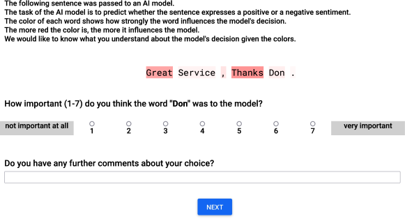
Figure 2. Screenshot of the importance rating interface for English sentiment sentences using saliency visualization.

Research Question. The core research question in this work is to probe into which, if any, factors in the explanation process—aside from the saliency itself—may influence the explainee’s interpretation of the saliency information. Formally, we view the saliency explanation as a process whose result is the explainee’s interpretation of the saliency scores. The “input” to this process is the original text as well as the saliency information and the visualization method. Then, we ask which factors in the original text have statistically significant effects on the explainee’s interpretation and how properties of the saliency score and the visualization method affect it.

Notably, a key challenge in analyzing the explainees’ saliency understanding is that we want to identify influencing factors on the explainee’s ratings without the existence of an inherently correct ground truth perception.

Proposed Methodology. We propose a combination of study design and statistical analysis to quantify the influence of arbitrary factors such as word length, sentiment polarity or dependency relations. We collect explainees’ subjective interpretations of the saliency scores in a crowdsourcing setup. We relate this interpretation to the original explanation considering various potentially influencing factors using an ordinal generalized additive mixed model (GAMM). The result from this comparison is an answer on which of the a-priori candidate explanatory factors indeed have significant effect on the explainee’s interpretation and how these factors functionally affect interpretation.

4. Study Methodology Specification

The study consists of two phases: collecting subjective importance interpretations (Section 4.1), and analyzing responses with an adequate statistical model (Section 4.3). We release the the collected data and analysis code.

4.1. Collecting Self-Reported Importance Ratings

In our main study, we investigate the interpretation of color-coding saliency visualization of the feature-attribution by crowdsource laypeople (variations on this study will be described later). We measure the perceived importance of a word within a saliency score explanation by directly probing human self-reported word importance. In this instance, we ask “How important (1-7) do you think the word "X" was to the model?” (Figure 2). We collect answers on a single-item unipolar 7-point Likert scale ranging from not important at all to very important.
Texts.  We use sentences from the Universal Dependencies English Web Treebank (Silveira et al., 2014). This treebank contains comprehensive annotation, including dependency relations of sentences, stemming from various domains such as newsgroups or online reviews. We use sentences from the reviews group for a plausible framing of a sentiment analysis task. We randomly select 150 sentences to be used.
Saliency Scores.  We assign random saliency scores to each token to uniformly sample the space of saliency intensities. We are, at this stage, not interested in using a “real” model or saliency score (e.g., attention or integrated gradients), as we investigate general perception of arbitrary scores. It is therefore useful to create saliency scores that “do not make sense” because a saliency score should reflect the model’s reasoning which might very well not make sense at all. We study an instance of “real” saliency scores (integrated gradients) later in Section 5.3.
Study Interface.  See Figure 2 for the rating collection interface. We display all sentences using monospaced font and fixed whitespaces to obtain a direct mapping between the number of characters and the color area for each word.
Procedure.  We ask participants to rate the importance of a randomly-selected word in the sentence. We show all 150 sentences from the described review dataset to each participant, displayed in a randomized order per participant. Saliency scores for all tokens are randomized for each participant (such that we collect responses to many different saliency maps, rather than numerous responses for the same set). We do so because our aim is not to obtain accurate (mean) estimates of single ratings as one would do in a corpus annotation, but to collect rich data to build an accurate model describing the underlying general phenomenon. For each sentence, we collect the participant’s importance rating, the completion time and a voluntary free-text comment. We choose to not include a dedicated training phase, e.g., showing the participants ten explanation instances before starting the data collection: we are explicitly interested in potential learning effects. These can be crucial in real-world applications: for example, should we find a decaying learning effect, an effective model audit should make sure to include a sufficient number of model predictions.
Participants.  We recruit 50 crowdworkers on Mechanical Turk. One crowdworker failed all of the trap sentences, so we exlude this worker’s responses and recruit one additional worker. All other participants successfully passed all trap sentences. In total, this yields 7500 importance ratings.

4.2. Factors of Saliency Perception

For our set of possible candidate factors, we model factors which are motivated by the three types of biases: anthropomorhic and belief biases, visual biases, and learning effects. Each factor will be tested for statistical significance on the explainees’ interpretations. Table 1 lists the factors we investigate in this work.

Selected factors in Table 1 include: (i) word length as longer words correspond to a larger colored draw area, which we hypothesize influences visual perception bias; (ii) word polarity as we present participants a sentiment classification task and expect that the participants’ own assessment of word importance influences their perception of how important it is to the model, which we hypothesize is an instance of belief bias; (iii) display index as we hypothesize that participant ratings are affected by temporal effects such as learning; (iv) word position as we hypothesize that, e.g., words at the center of a sentence might be perceived more strongly due to the center bias (visual perception bias) which was observed in various eye-tracking studies, i.a., for natural scenes (Tseng et al., 2009).

Table 1. List of factors that presupposedly affect saliency explanation perception along with the findings of our three user studies. EN refers to the English sentiment classification study, DE to the German fact checking study and EN-IG to the English sentiment classification study using integrated gradients as feature attribution method (without correction visualizations).

Factor	Description	Significant Effects
		EN	DE	EN-IG
Saliency	The color intensity specified as the saturation value ($S\in[0,1]$) in a $(H,S,V)$ color triple (Smith, 1978), e.g., (0°,0.5,1.0) ($\blacksquare$) and (0°,0.25,1.0) ($\blacksquare$).	✓	✓	✓
Word length	The number of characters in a word, e.g., 7 for “example”.	✓	✓	✓
Word frequency	The word’s normalized frequency, estimated on a large corpus.			✓
Sentence length	Number of words in the sentence.	✓	✓
Display index	The sentence’s position within a sequence of sentences (e.g., the third sentence in the sequence of 150 sentences). This relates to temporal effects such as learning.	✓	✓
Sentiment polarity	The sentiment polarity of a word (defined via its lemma) $\in[-1,1]$.	✓	–
Saliency rank	Normalized rank of a word’s saliency score (i.e. color intensity) in comparison to the other words in its sentence $\in[0,1]$.	✓		✓
Word position	The index of the token’s position within its sentence.		✓
Capitalization	The word’s capitalization, e.g., “example”, “Example” or “EXAMPLE”.		✓
Dependency relation	Dependency relation to its parent within the dependency graph (36 types for EN).		✓

4.3. Statistical Analysis Using GAMMs

Given a set of inputs for which there are the feature-attribution scores, and the interpreted importance scores, we describe the analysis methodology aiming to derive the possible input factors that cause discrepancy between the two.

4.3.1. Ordinal Generalized Additive Mixed Model

We analyze the collected ratings of perceived importance using a ordinal generalized additive mixed model (GAMM). Its key properties are that it (i) models the ordinal response variable (i.e., the importance ratings in our setting) on a continuous latent scale (ordinal generalized), which is (ii) modeled as a sum of smooth functions of covariates (additive) and (iii) accounts for random effects (mixed). The continuous latent scale is linked to ordinal categories by estimating threshold values that separate neighboring categories. The smooth functions can comprise single covariates (univariate smooths) such as $f_{1}(x_{1})$ or combinations of multiple covariates such as $f_{2}(x_{2},x_{3})$. Random effects allow to account for, e.g., systematic differences in individual participants’ rating behaviour. For example, a specific participant might have a tendency to give overall higher ratings than other participants. Including a random effect allows to disentangle this influence on the response variable from the influence of the covariates in question (such as word length) and thereby offers a clearer view on these fixed effects. The GAMM analysis enables us (i) to make statements about which factors significantly influence saliency perception, without prescribing any notion of “correct perception” and (ii) to study the relation between these factors and participants’ importance ratings in detail, via an interpretation of the model’s parametric terms (categorical factors) as well as smooth terms (numeric factors). We provide a description of each of the ordinal GAMM’s components in Appendix A.

4.3.2. Model Details

We include all factors listed in Table 1 into our model formula. We use smooth terms for numeric factors and parametric terms for categorical factors. Additionally, we include tensor product interactions for all pairs of smooth terms. In order to statistically account for potentially confounding effects of individual participants or sentences, we include random intercepts as well as random slopes for each participant and each sentence. Before fitting the model, we remove a small amount of outlier ratings. We use fast REML for smoothness selection and apply variable selection via double-penalty shrinkage (i.e., additionally penalizing the splines’ null space). We fit the model using discretized covariates as described in Wood et al. (2017) and Li and Wood (2020).

5. Study Results, Interpretation and Generalizations

In the following, we conduct three user studies. The first study (Section 5.1) investigates saliency perception for English and a sentiment classification task. The second study (Section 5.2) extends the investigation to German language and a fact checking task to evaluate generalization of the findings. Since these two studies use random saliency scores so as to not prescribe a specific feature-attribution method, we report a third study (Section 5.3) which uses the wide-spread integrated gradient scores as a generalization to practically-used attribution methods.

5.1. Sentiment Analysis in English

We discuss quantitative results based on the fitted GAMM (Section 5.1.1) as well as qualitative findings based on the participants written feedback (Section 5.1.2).

5.1.1. Quantitative

Table 2 shows statistics for the univariate smooth terms in the fitted GAMM. Figure 3 shows partial effect plots of the respective significant smooth terms.

Table 2. Effective degrees of freedom (edf), reference df and Wald test statistics for the uniariate smooth terms of the first user study.

	edf	ref. df	F	p
s(saliency)	12.0967	19	728.8738	$<$ 0.0001
s(display index)	1.0921	9	2.0872	0.0001
s(word length)	2.5416	9	4.1826	$<$ 0.0001
s(sentence length)	0.9200	9	1.7531	0.0001
s(word frequency)	0.0011	9	0.0001	0.1082
s(sentiment polarity)	2.1281	9	1.6156	0.0065
s(saliency rank)	0.9580	9	4.4417	$<$ 0.0001
s(word position)	0.0005	9	0.0000	0.7882

Regarding the parametric terms, neither a word’s capitalization (df=2, F=1.84, p=0.16) nor its dependency relation (df=35, F=1.17, p=0.24) show a significant effect on perceived importance. Regarding the smooth terms, we observe that saliency score, display index, word length, sentence length, word sentiment polarity and saliency rank show significant effects on perceived importance. In the following, we discuss each effect in detail.
Saliency (Figure 3(a)):  The saliency (i.e., the color saturation) has the strongest impact on perceived importance as the graph spans the by-far widest y-axis range of all plots in Figure 3. Except for the saliency scores around 1, the entire graph shows a monotonous relation between saliency score and perceived importance.
Display Index (Figure 3(b)):  Participants’ ratings increased over the course of the experiment. We hypothesize that the participants report more conservative ratings in the beginning of the experiment to “leave enough room” for more extreme sentences and adapt their ratings to a more “calibrated” level over the course of the experiment. Interestingly, this trend does not seem to stop after our maximum number of 150 sentences. We leave the study of sufficient amount of training required for the effect to reach a peak to future work.

(a) Saliency (saturation)

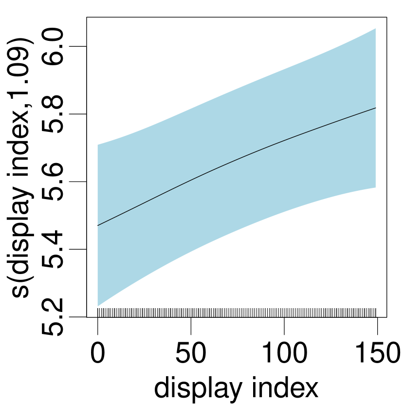
(b) Temporal display index

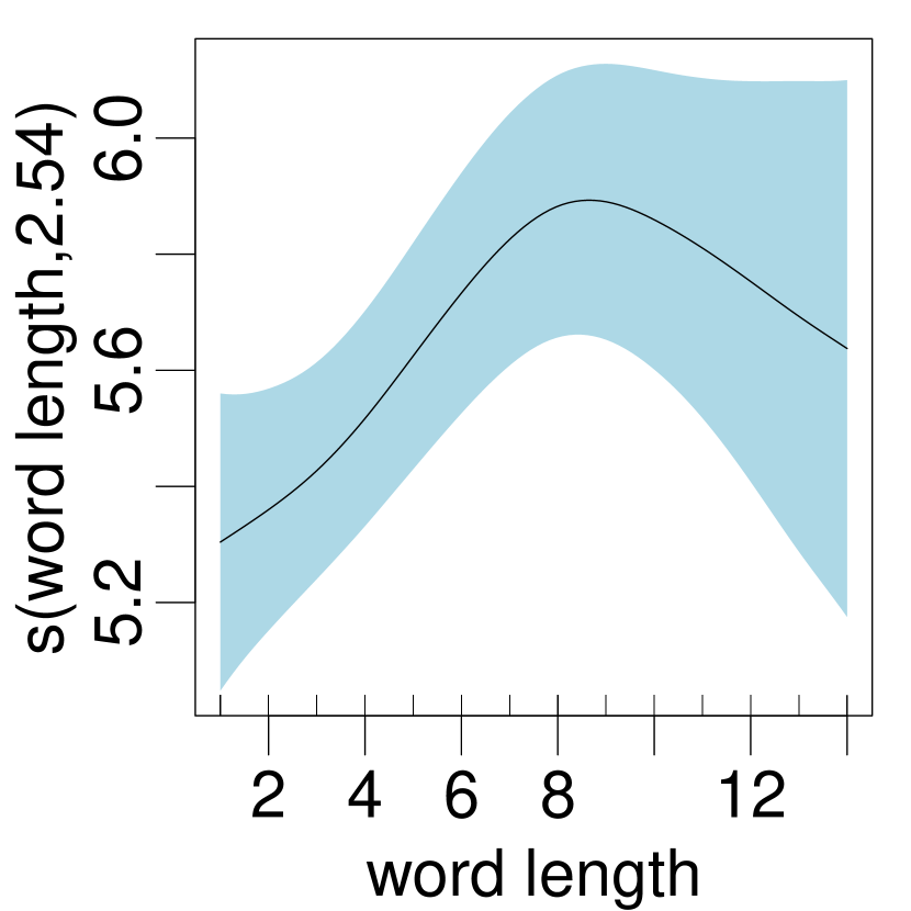
(c) Word length

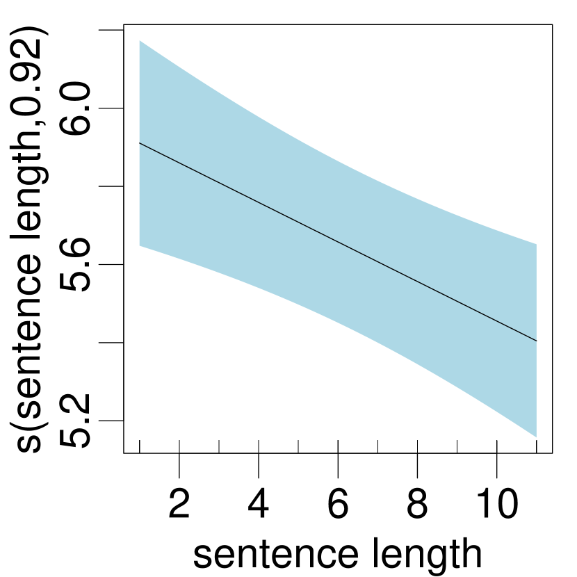
(d) Sentence length

(e) Word sentiment

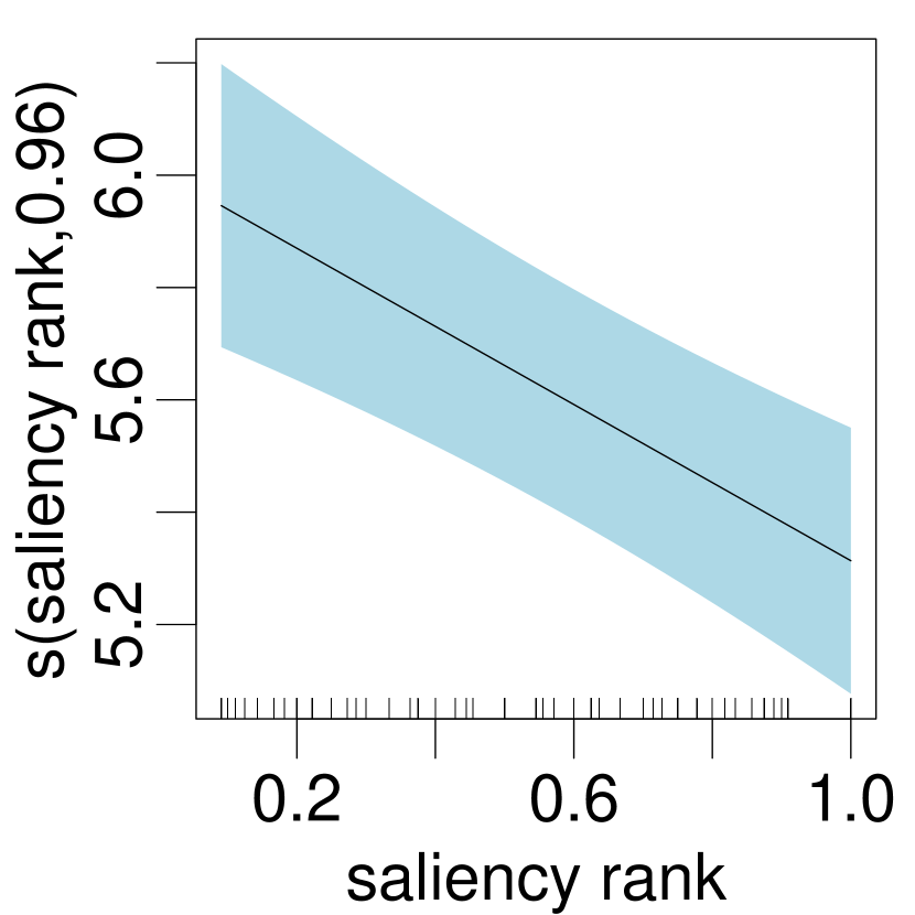
(f) Saliency rank

Figure 3. Partial effect plots for all significant smooth terms (note that y-axes are scaled per effect). Numbers in y-axis labels are estimated degrees of freedom (edf) of the respective smooth. The shaded area displays confidence intervals (plus and minus one standard error) including uncertainty about the overall mean.

Word Length (Figure 3(c)):  With increasing word length, importance ratings rise up until a length of approximately eight characters and decrease again afterwards. We hypothesize that the initial increase corresponds to an increase of the colored area that a longer word directly causes, as the saliency score is visualized within a box which is proportional to the number of characters. To interpret the subsequent decrease of perceived importance, we consider the interactions between word length and other factors. We find significant pairwise interactions of word length with (i) saliency, (ii) display index and (iii) word frequency (Appendix C). For the interaction with display index, we observe that the decreasing effect of high word lengths grows with increasing display index up until around the 55th sentence. After this point, the effect decreases. While the latter decrease can be explained with the partial effect of increasing ratings with higher display indices (as shown in Figure 3(b)), the former decrease demands detailed investigation in future work.
Sentence Length (Figure 3(d)):  Importance ratings decrease for words in longer sentences. A longer sentence leads to a higher number of color samples and therefore also to a larger expected color range. We argue that such an increased color range inhibts users to make very high importance ratings due to a missing “maximum color” anchor.
Sentiment Polarity (Figure 3(e)):  The effect of a word’s lemma’s sentiment polarity on importance ratings. We observe a parabola-shaped curve with a minimum at slightly-positive sentiment. To the left, importance ratings increase with increasingly negative polarity and to the right importance ratings increase with increasingly positive polarity. This indicates that users ratings of “what was important to the model when classifying the sentence” are biased by their answer to “what is important to me when classifying the sentence myself”. Such a substitution of a presumably complex-to-compute target attribute with a simpler heuristic attribute is a known cognitive bias and often referred to as attribute substitution or substitution bias (Kahneman and Frederick, 2002)
Saliency Rank (Figure 3(f)):  The partial effect of a word’s normalized saliency rank on participants’ importance ratings. We normalize the rank by dividing by sentence length, as low ranks (i.e., larger numbers) would otherwise be strongly correlated to sentence length, and potentially cause stability issues within the model estimation. We observe that an increased rank (a value of one corresponds to the last rank, i.e., the lowest saliency score) corresponds to a decrease in rated importance. In contrast to the effect of saliency score shown in Figure 3(a), the saliency rank is not only a property of a word but of a word in context of its sentence. A word’s saliency score can remain unchanged while at the same time its rank can be arbitrarily modified by changing the saliency scores of the other words in its sentence. We argue that the significant effect of saliency rank indicates that users interpret saliencies in relation to each other, i.e., their judgements are relative and lack a fixed anchoring point. This is supported by qualitative analysis in Section 5.1.2.

In addition to the significant partial effects, we also find numerous significant interactions. We provide the statistics of Wald tests for all pairwise tensor product interactions (following a functional ANOVA decomposition) as well as summed effect plots of all significant pairwise interactions in Table 5 and Figure 10 in Appendix C.

5.1.2. Qualitative

In addition to the statistical evaluation, we also evaluate the participants’ voluntary free-text comments. Table 3 shows a selection of comments grouped into four categories:
Relative Judgement:  Participants explicitly state that they make relative importance judgements. This supports our argumentation of relative judgments discussed for the effects of sentence length and saliency rank.
Own Opinion:  Similarly, participant comments support our hypothesis that users’ ratings are subject to the cognitive bias of attribute substitution as discussed for the effect of word sentiment polarity.
Light Color:  Participants seem to make a categorial distinction between very light color and seemingly no color although this distinction does not exist in terms of the attribution score. This can be important when communicating very low influences and should be addressed in more detail in future work.
Other:  Miscellaneous comments on, e.g., issues of word-level attribution and the resulting ambiguity in interpretation.

Table 3. Comments of the participants of the English sentiment study. Participants were asked to rate the underlined word or symbol.

5.2. Generalization Across Tasks and Languages: Fact Checking in German

So far, we found indication that numerous factors (word length, saliency rank, etc.) significantly influence users’ subjective importance ratings. Two important limitations are that (i) the findings are limited to English, and (ii) they are limited to one AI task (sentiment classification). To assess whether the findings do generalize to another language and another task, we repeat the study identically with German sentences from the PUD Corpus with a fact checking AI task. We collect responses from 25 German-speaking participants from a participant pool including Germany, Austria and Switzerland. In total, this corresponds to 3750 ratings.

5.2.1. Confirmed Effects

Our analysis confirms the significants effects of saliency, display index, word length and sentence length. Figure 4 displays the respective partial effect plots. While the smooths for saliency (Figure 4(a)) and sentence length (Figure 4(d)) show high similarity to the respective smooths of the English study (see Figures 3(a) and 3(d)), we observe slight differences for display index (Figures 4(b) and 3(b)) and word length (Figures 4(c) and 3(c)). While the English display index smooth grows more or less linearly (edf=1.09), the respective German smooth reaches a plateau after around half the sentences (edf=1.60). We hypothesize that such a saturation effect will also be visible for English, but requires a larger number of sentences. We argue that this is caused by the fact that the sentences in the German study are longer than in the English study, which makes participants of the German study see more colored words and thereby “calibrates” their ratings faster in terms of number of sentences. Similarly, the German word length smooth saturates after around 15 characters, while the English smooth decreases after around 8 characters. We hypothesize that this difference can be attributed to the overall longer words in German as well as the difference in compounding.

The effect of saliency rank cannot be confirmed in the German experiment. Like in the English study, we find no indication that word frequency has a significant effect on importance ratings. We provide test statistics of paramatric and smooth terms (univariate smooths and pairwise interactions) as well as coefficient estimates in Appendix D.

As in the English study, we additionally qualitatively analyse the participants’ free text comments and observe (as in the English study) numerous instances for which participants mix their own estimate of importance with the communicated importance. We provide exemplary instances in Table 9 in Appendix D.

5.2.2. Additional Effects

In addition to the effects that we already observed in the English study, we also find that the word’s position within the sentence (Figure 4(e)) as well as capitalization and dependency relation have significant effects on importance ratings. A full list of coefficient estimates along with further details is provided in Table 8 in Appendix D.

The estimate for fully capitalized words is 1.91 (SE=0.9638), the respective estimate for words with the first letter capitalized is 0.41 (SE=0.12). This confirms the intuition that fully capitalized words receive the highest importance ratings, followed by first-letter-capitalized words. We argue that this effect—in particular for first-letter-capitalized words—is more visible in the German experiment as German uses more frequent capitalization (e.g., for all nouns).

Regarding dependency relations, the highest estimate can be observed for temporal modifiers (obl:tmod, $\beta=1.70$, SE=0.55) like “today” and numerical modifiers (nummod, $\beta=1.39$, SE=0.36) like “one”. The lowest estimate can be observed for clausal modifier of nouns (acl, $\beta=-1.22$, SE=0.64) like “sees” in “the issues as he sees them” and indirect objects (iobj, $\beta=-0.48$, SE=0.52) like “me” in “she gave me the book”. We hypothesize that the grammatical function effect is larger here than in the previous experiment because properties such as the use of temporality, numerals and embedded clauses are more important for determining factuality than for determining sentiment.

(a) Saliency (saturation)

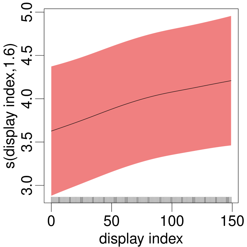
(b) Temporal display index

(c) Word length

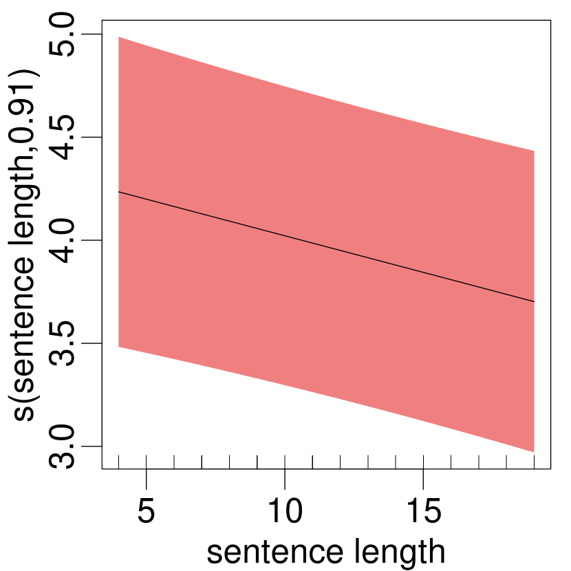
(d) Sentence length

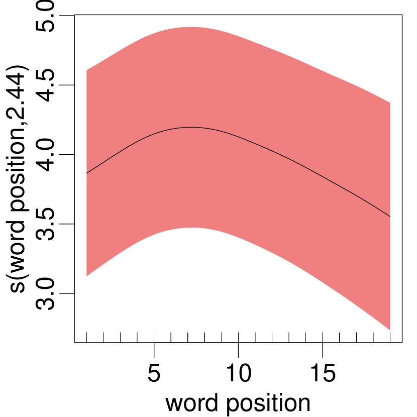
(e) Word position

Figure 4. Partial effect plots for all significant smooth terms (note that y-axes are scaled per effect) for the German experiment. Numbers in y-axis labels are estimated degrees of freedom (edf) of the respective smooth. The shaded area displays confidence intervals (plus and minus one standard error) including uncertainty about the overall mean. (a) refers to color saturation.

5.3. Generalization to Model-based Saliencies (derived via Integrated Gradients)

We want to assess whether our findings on the random saliency scores used in the previous two studies also hold for practically-used feature attribution scores. Therefore, we conduct an additional user study using integrated gradients (Sundararajan et al., 2017) instead of random saliencies.

5.3.1. Study Modification: Within-Subject Design

We combine the evaluation of integrated gradient scores with a within-subject evaluation of three visualization methods which we detail in Section 6. In this section, we focus on the unmodified visualization as it is used in the two previously described studies. In the remainder of this paper, this visualization method is referred to as saliency. We sample another 150 sentiment sentences from the sentence pool described in Section 4.1 and present them in the same sentiment classification context. Instead of using one saliency visualization method for all 150 sentences, we now use the three visualizations and show each participant 50 sentences per visualization. We collect 9000 importance ratings from 60 participants and exclude participants of the previous study to avoid carry-over effects from previous exposures.

5.3.2. Model Modification: Factor-Smooth Interactions

We again use an ordinal GAMM model using the same covariates as described in Section 4.3. In addition, we add a parametric term for the visualization condition to account for overall differences in rating intensities between the visualization conditions. We use factor-smooth interactions for each variable which leads to separate estimates for each variable per visualization (e.g., three smooths for word length, one per visualization). First, this yields smooths for the “orginal” saliency visualization, i.e., the heatmap visualization without saliency corrections. In contrast to our first study, these smooths now correspond to effects on integrated gradient attribution scores instead of random scores. First, comparing the smooths allows us to compare how factors influence importance ratings across the three visualizations, e.g., to assess whether the bar visualization did mitigate the biasing effect of word length. We discuss the respective results in Section 6.3. Second, analyzing the smooths relating to the original saliency visualization allows us to evaluate which of the effects we observed in the first study do generalize to the integrated gradients attribution scores. We discuss the respective results in the following paragraph.

5.3.3. Results

We find significant effects of saliency score, word length, relative word frequency and saliency rank. We provide details and test statistics on all parametric coefficients as well as smooth terms in Table 12 in Appendix F. All of these variables except relative word frequency were also found to be significant in our first study and all of them except relative word frequency and saliency rank were confirmed in our German study. The significant influence of relative word frequency was observed for the first time.

Overall, three studies confirmed the presumably biasing influence of word length, (pairs of) two studies respectively confirmed the effect of sentence length, display index and saliency rank, and one study (each) found significant effects of word position, sentiment polarity, word frequency, capitalization and dependency relation. Together, these reflect the three sources of bias: anthropomorphism and belief bias, visual perception, and learning effects.

6. Mitigating Visual Perception and Learning Effect Biases

So far, we observed that various seemingly irrelevant factors influence human perception in unintended ways from the explicit and objective saliency information across different languages, tasks and feature-attribution scores. Next, we explore two methods to decrease the bias in human perception (Figure 5): (i) controlling for the bias by modifying the color-coding to account for over-estimation and under-estimation of importance (over-estimated tokens will receive decreased color saturation, and vice versa); (ii) replacing the color-coding visualization with bar chart visualization.

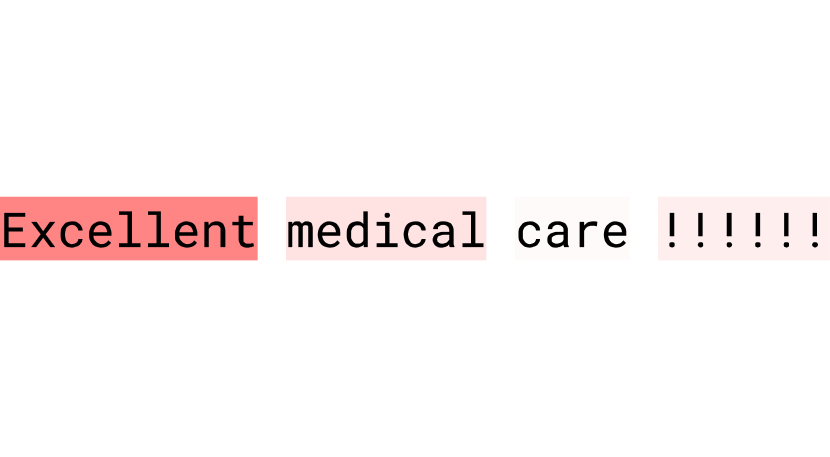
(a) Original saliency

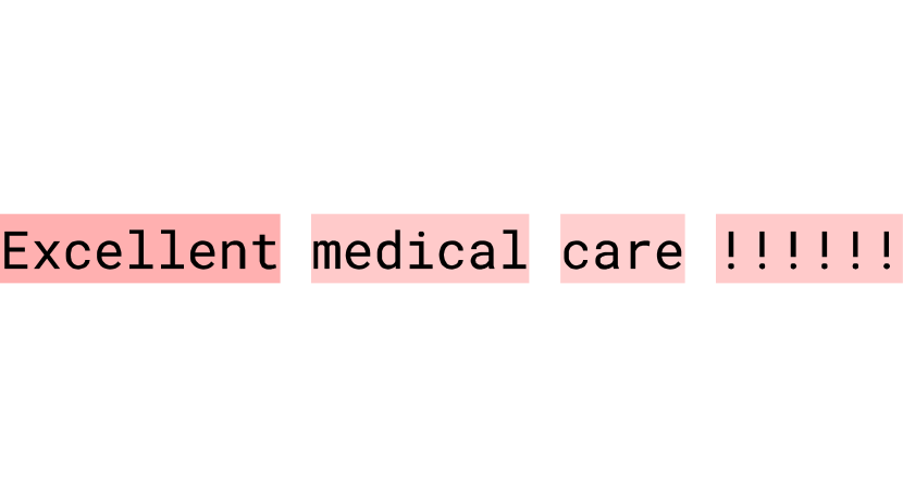
(b) Corrected saliency

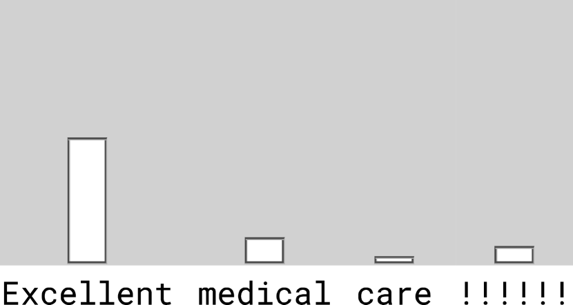
(c) Bars

Figure 5. The three different visualization methods we compare in our third study (Section 6).

6.1. Model-Based Color Correction Technique

We compute an alternative color-coding visualization which a-priori accounts for over-estimation and under-estimation of tokens based on the data collected in the previous experiments. Here we investigate whether it is possible to “correct” the explainees’ saliency perception by superimposing the initial saliency values with a correction signal.

We require a procedure which increases the saliency scores for words which are predicted to be under-perceived (e.g., short words and words that appear in long sentences) and decrease the saliency scores for words that are predicted to be over-perceived (e.g., words with a high sentiment polarity or words that appear in short sentences). Briefly, the trained GAMM model from the English study (Section 5.1) allows us to map a combination of a saliency score together with word/sentence properties to a perceived importance score (on a continuous latent scale). By grounding this prediction of perceived importance to a prediction conditioned on a particularly chosen reference level, we can iteratively, globally correct the explained scores over the sentence such that the (predicted) perception bias is decreased in each iteration. Table 4 displays examples of the application of this correction. In Appendix E, we discuss the full algorithm including its components and motivating details and provide an extended list of example applications in Table 11 as well as an example of the gradual correction of one sentence over the course of 100 correction steps in Table 10.

6.2. Bar Chart Visualization

As an alternative to color-coding visualization, we consider bar charts (Figure 5(c)): we investigate whether a sufficiently distinct visualization will result in different perception. We hypothesize that this is related to visual perception bias.

We note two visual qualities of bars which differentiate it from color-coding, and therefore make it a relevant alternative visualization candidate: (i) The bars are communicated with objective reference points of 0 and 1 (the top and bottom of the draw area), while the results in Section 5.1 indicate that participants perceive colored saliency in relation to each other, instead of in reference to 0 and 1 (pure white and pure red, respectively); (ii) The draw area for the bars is separate from the draw area for the input text, in contrast to color-coding, where they occupy the same space. This means that in color-coding, for example, a word with more characters will receive a larger area of color, in comparison to a shorter word with the same color. As our studies in Section 5 show, word length influenced explainee perception. In the bar chart visualization scheme, all words are treated identically within the draw area which communicates importance, and this draw area is disconnected from the text display area.

6.3. Results

Table 4. Examples of the bias reduction procedure. The saliency column shows the saliency explanations (how users would see them) before and after the bias correction procedure. The bias column shows the color-coded bias estimates. Predicted over-estimations are in red whereas predicted under-estimations are in blue. More examples in Table 11 in Appendix E.

We investigate how well the two proposed visualization alternatives counteract bias in user perception within the study described in Section 5.3. We find that visualization has a significant effect on importance ratings (df=2, F=35.45, p<0.0001) where the bar visualization leads to lower importance ratings ($\beta=-0.5991$, SE=0.1579) and the correction visualization leads to higher importance ratings ($\beta=1.1102$, SE=0.2515). Regarding the visualizations’ effect on smooth terms, we focus on the smooths for color saturation, word length and display index in Figure 6.

Figure 6(a) shows that the saliency scores’ effect on importance ratings is similar to the original saliency and the bar visualizations, while the corrected visualization leads to higher importance ratings in the lower end of the color saturation spectrum. These differences are neither “good” nor “bad”—we argue that the similarity between the original saliency visualization and the bar visualization is remarkable as the two visualizations are fundamentally different.

Figure 6(b) shows that the biasing effect of word length in the original visualization is successfully eliminated using the bar visualization as shown by the nearly constant smooth of the bar visualization (edf=0.0009). This confirms our hypothesis that a bar visualization evades word length bias. The correction visualization leads to a different effect than the original visualization, however, this effect indicates a different but equally distorting bias of word length.

Figure 6(c) indicates a successful application of our color correction technique. While the original visualization as well as the bar visualization show a biasing effect regarding the model smooths, the saliency correction visualization leads to a nearly constant smooth (edf=0.0009). Regarding the original and the bar visualizations, the smooths indicate that, in contrast to the original visualization, the bar visualization leads to an initial overestimation of importances which decreases over time, while the original visualization lead to a respective underestimation. However, a difference plot between the two conditions (see Figure 12(c) in Appendix F) shows no significant differences.

While these examples demonstrate indications for successful bias mitigation, we want to note that this mitigation cannot be observed for most of the other variables, in particular not for the effect of saliency rank, which we expected to be mitigated by the bar visualization.

Tying back to our initial categorization of biases, we observe that our proposed visualization alternatives can successfully remove instances of visual bias (word length) and learning effect bias (display index).

(a) Saliency

(b) Word length

(c) Temporal display index

Figure 6. Selected summed-effects comparison plots of the visualization alternatives.

7. Conclusion

We analyze feature-attribution for text from a novel, arguably under-explored perspective: we investigate how humans interpret saliency explanations over text and which factors affect their perception. We show that there can be discrepancy between the communicated information and how it is interpreted, even for a straight-forward and explicit explanation medium of feature-attribution for text. This is achieved through a general methodology for investigating which factors in the input may cause this discrepancy. We demonstrate the methodology for a lay-people audience of crowd-workers over multiple tasks, languages and visualizations, showing different setups yield similar but distinct distortions. We find that word length, sentence length, learning effects, and within-sentence saliency relations affect human importance ratings across multiple user studies. The methodology can and should be used on other audiences and tasks, before trusting a saliency visualization for this audience/task pair. We present two bias correction methods and demonstrate their ability to compensate the distorting influence of word length and repeated exposure. Our findings inform future design of saliency visualizations towards closing the gap between communicated and interpreted saliency explanations, and call for further research in the human factors in interpretation methods of AI, that study not only how the AI operates, but how humans perceive the communicated information.

Appendix A Brief Introduction to Ordinal GAMMs

For an intuitive understanding, we sketch how one arrives at ordinal generalized additive mixed models (GAMMs) starting from linear models. We follow notation by Wood (2017).

Linear Model. In a linear model, the response variable $\mathbf{y}$ (e.g., a numeric rating of importance) is modeled as a function of explanatory variables $\mathbf{X}$ which are related to $\mathbf{y}$ linearly via parameters $\mathbf{\beta}$ assuming additional noise $\mathbf{\epsilon}$:

(1) $$\mathbf{y}=\mathbf{X}\mathbf{\beta}+\mathbf{\epsilon}.$$

Linear Mixed Model. In many scenarios, there are random effects which one wants to account for in the model. For example, we collect 150 word importance ratings per participant, i.e., we collect repeated measures and are at danger of violating the independence assumption and introducing a confounding effect of the variable participant ID because specific participants might have a tendency to give overall higher ratings than other participants. Like the linear model, linear mixed models estimate fixed effects but in addition they also model random effects (e.g., of the participant ID) to disentangle their influence on the response variable and thereby offer a clearer view on the fixed effects. The general formulation of a linear mixed model reads

(2) $$\mathbf{y}=\mathbf{X}\mathbf{\beta}+\mathbf{Z}\mathbf{b}+\mathbf{\epsilon},$$

where $\mathbf{Z}$ corresponds to the random effects and $\mathbf{b}$ to the respective weights.

Generalized Linear Model (GLM). While linear models require the response distribution to be normal, generalized linear models (Nelder and Wedderburn, 1972) generalize to non-normal (exponential family) response distributions such as categorical responses (e.g., dog or cat) or ordinal responses (e.g., Likert item ratings). To achieve this generalization, GLMs link values on the response scale (e.g., categorial ratings) to a latent scale (e.g., logits) via a link function $g(\cdot)$ (e.g., logit function): For a row $i$, the general formulation reads:

(3) $$g(\mu_{i})=\mathbf{X}_{i}\mathbf{\beta}.$$

Generalized Additive Model (GAM). While a generalized linear model only allows to model linear relationships between the the explanatory variables and $g(\mu_{i})$, a GAM (Hastie and Tibshirani, 1990) generalizes the linear relationship to a sum of smooth functions of explanatory variables using:

(4) $$g(\mu_{i})=\mathbf{X^{*}}_{i}\mathbf{\theta}+f_{1}(x_{1i})+f_{2}(x_{2i},x_{3i})+...\ ,$$

where $f_{1}$ and $f_{2}$ are smooth functions that typically are chosen to be a sum of basis functions, such as splines and $\mathbf{X^{*}}$ corresponds to strictly parametric model components. A regularized estimation of these functions allows GAMs to model complex functions, but also to fall back to simpler, e.g., constant or linear functions when an increase in model complexity is not sufficiently warranted by improved model fit.

Ordinal Generalized Additive Mixed Model (ordinal GAMM). Having introduced the previous models, an ordinal GAMM can be described as a generalized additive model that additionally accounts for random effects and models ordinal ratings via a continuous latent variable that is separated into the ordinal categories via estimated threshold values. For further details, Divjak and Baayen (2017) provide a practical introduction to ordinal GAMs in a linguistic context and Wood (2017) offers a detailed textbook on GAM(M)s including implementation and analysis details.

Appendix B Study Interfaces

In addition to the screenshot shown in Figure 2, Figure 7 shows the interface of the German study and Figure 8 shows an interface that uses the alternative bar chart visualization. Figure 9 displays one of the three trap questions we use to detect participants that do not pay attention to the task.

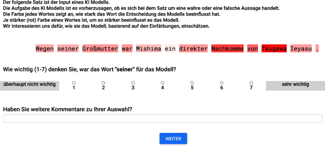
Figure 7. Screenshot of the importance rating interface for German fact checking sentences using saliency visualization.

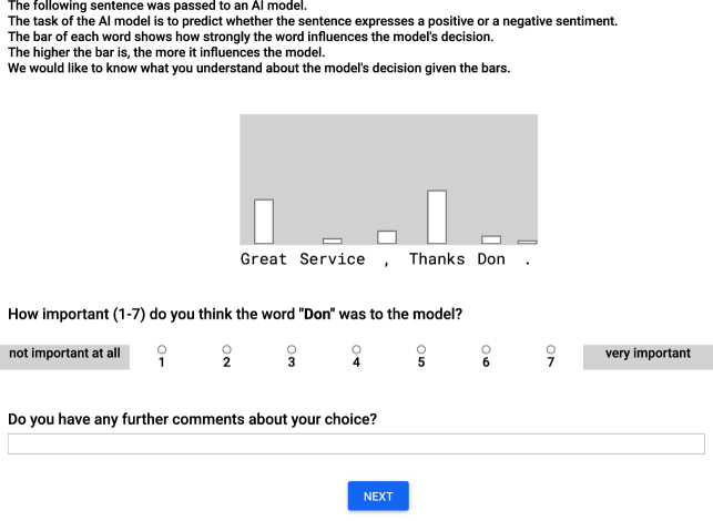
Figure 8. Screenshot of the importance rating interface for English sentiment sentences using bar visualization.

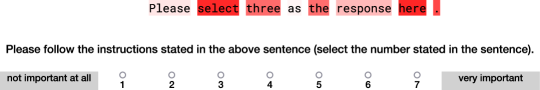
Figure 9. Screenshot of one of three trap sentences used to validate that the participant pays attention to the task.

Appendix C English Study Details

Table 5 displays test statistics for all smooth pairwise interactions. We make use of tensor interaction smooths following a functional ANOVA decomposition. Figure 10 shows summed effect plots for the respective significant interactions. Ordered categorial cut points are located at -1, 1.31, 3.29, 5.15, 7.1 and 9.22.

Table 5. Wald tests for the pairwise interactions (tensor interactions) (upper) and random effects (lower) of the English user study.

	edf	ref. df	F	p
ti(saliency,display index)	2.5102	16	2.1075	0.0001
ti(saliency,word length)	6.0566	16	2.2698	0.0001
ti(saliency,sentence length)	3.1609	16	1.1203	0.0020
ti(saliency,word frequency)	0.9176	12	1.8325	0.0004
ti(saliency,sentiment polarity)	2.9357	16	0.5553	0.0814
ti(saliency,saliency rank)	0.0004	16	0.0000	0.5864
ti(saliency,word position)	0.6254	16	0.1144	0.1276
ti(display index,word length)	1.5112	16	0.6637	0.0026
ti(display index,sentence length)	1.2776	16	1.0159	0.0010
ti(display index,word frequency)	2.6938	16	1.7810	0.0001
ti(display index,sentiment polarity)	0.5386	16	0.0853	0.1678
ti(display index,saliency rank)	1.3966	16	0.5272	0.0174
ti(display index,word position)	3.3649	16	0.6625	0.0520
ti(word length,sentence length)	0.0004	16	0.0000	0.9236
ti(word length,word frequency)	2.1540	16	6.5510	$<$ 0.0001
ti(word length,sentiment polarity)	0.0014	16	0.0000	0.6790
ti(word length,saliency rank)	2.2175	16	0.3503	0.0573
ti(word length,word position)	1.0296	16	0.1270	0.1222
ti(sentence length,word frequency)	0.0005	16	0.0000	0.8608
ti(sentence length,sentiment polarity)	0.0013	16	0.0001	0.5113
ti(sentence length,saliency rank)	1.3045	16	0.2651	0.0453
ti(sentence length,word position)	3.1995	16	0.8487	0.0067
ti(word frequency,sentiment polarity)	0.0015	16	0.0001	0.1969
ti(word frequency,saliency rank)	0.0022	15	0.0001	0.3230
ti(word frequency,word position)	2.0375	16	0.3168	0.0924
ti(sentiment polarity,saliency rank)	0.0006	16	0.0000	0.8407
ti(sentiment polarity,word position)	0.0005	16	0.0000	0.9558
ti(saliency rank,word position)	0.0006	16	0.0000	0.6542
s(sentence_id)	0.0006	150	0.0000	0.9276
s(saliency,sentence_id)	9.1441	150	0.0676	0.2305
s(worker_id)	48.1065	49	10640.8475	$<$ 0.0001
s(saliency,worker_id)	48.0654	50	6593.7769	$<$ 0.0001

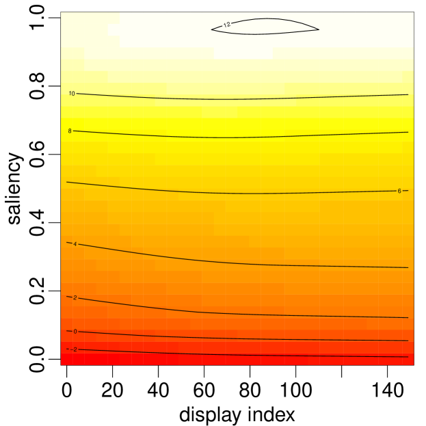
(a) Saliency * display index

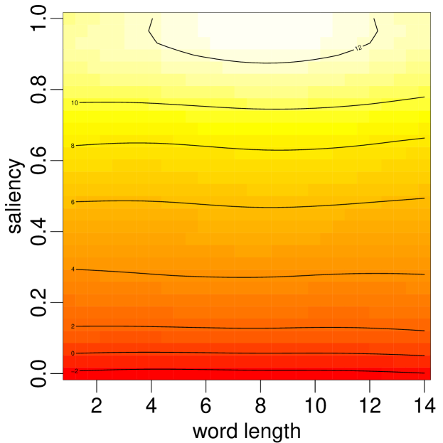
(b) Saliency * word length

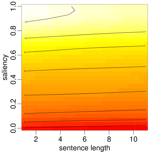
(c) Saliency * sentence length

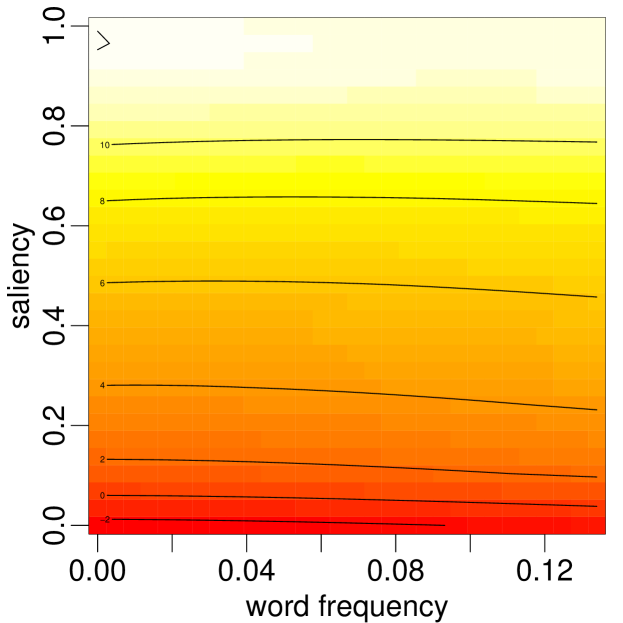
(d) Saliency * word frequency

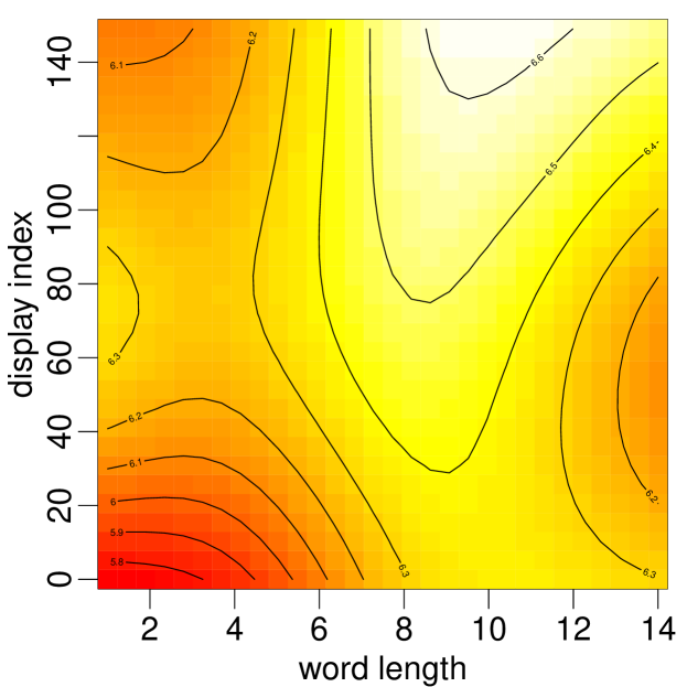
(e) Display index * word length

(f) Display index * sentence length

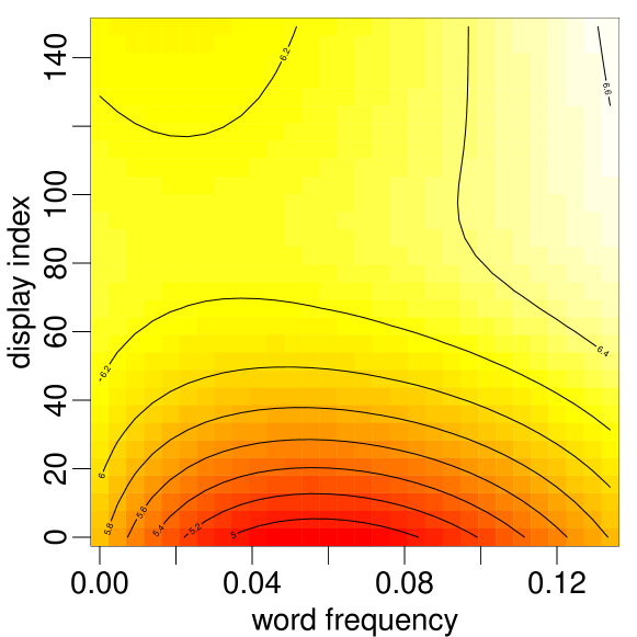
(g) Display index * word frequency

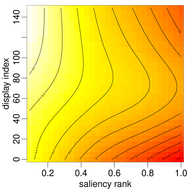
(h) Display index * saliency rank

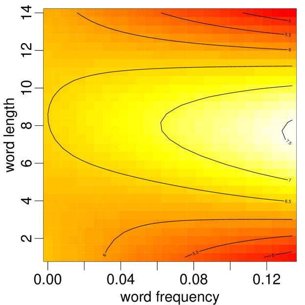
(i) Word length * word frequency

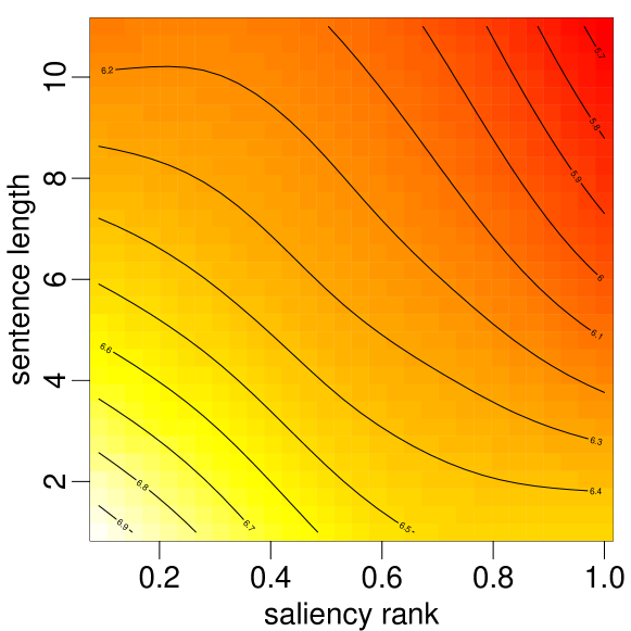
(j) Sentence length * saliency rank

(k) Sentence length * word position

Figure 10. Summed effect plots of all significant pairwise interactions.

Table 6. Wald tests for the parametric terms of the German user study.

	df	F	p
capitalization	2	7.62	0.0005
dependency relation	33	2.57	$<$ 0.0001

Table 7. Wald tests for the smooth terms of the German user study.

	edf	ref. df	F	p
s(saliency)	8.2052	19	148.1115	$<$ 0.0001
s(display index)	1.5999	9	2.4742	$<$ 0.0001
s(word length)	2.0440	9	3.9174	$<$ 0.0001
s(sentence length)	0.9073	9	1.7657	0.0003
s(word frequency)	0.0017	9	0.0002	0.2816
s(saliency rank)	0.0004	9	0.0000	0.7016
s(word position)	2.4429	9	2.8142	0.0002
ti(saliency,display index)	0.0007	16	0.0000	0.5846
ti(saliency,word length)	2.4114	16	1.1662	0.0013
ti(saliency,sentence length)	1.8496	16	0.7410	0.0125
ti(saliency,word frequency)	0.6953	11	0.3084	0.0549
ti(saliency,saliency rank)	1.4340	16	0.4958	0.0142
ti(saliency,word position)	0.0765	16	0.0053	0.2970
ti(display index,word length)	0.3529	16	0.0477	0.1968
ti(display index,sentence length)	0.1902	16	0.0171	0.2622
ti(display index,word frequency)	0.0005	15	0.0000	0.7096
ti(display index,saliency rank)	0.2967	16	0.0332	0.2325
ti(display index,word position)	1.1440	16	0.4244	0.0168
ti(word length,sentence length)	0.9858	16	0.3138	0.0290
ti(word length,word frequency)	0.9622	11	1.0293	0.0050
ti(word length,saliency rank)	0.0005	16	0.0000	0.8581
ti(word length,word position)	0.8285	16	0.5132	0.0091
ti(sentence length,word frequency)	0.0009	15	0.0001	0.3536
ti(sentence length,saliency rank)	0.0005	16	0.0000	0.9945
ti(sentence length,word position)	0.0005	16	0.0000	0.6862
ti(word frequency,saliency rank)	0.0003	16	0.0000	0.9438
ti(word frequency,word position)	0.0005	15	0.0000	0.6085
ti(saliency rank,word position)	0.0004	16	0.0000	0.8379
s(sentence ID)	0.0004	149	0.0000	0.9007
s(saliency,sentence ID)	36.6567	150	0.3534	0.0087
s(worker ID)	23.5324	24	8128.6327	$<$ 0.0001
s(saliency,worker ID)	23.6122	25	5645.0812	$<$ 0.0001

Table 8. Capitalization and dependency relation coefficients for the German user study.

Coefficients	$\beta$	SE	t	p
capitalization: all capital	1.9051	0.9638	1.9767	0.0481
capitalization: first capital	0.4074	0.1151	3.5390	0.0004
dependency relation: acl	-1.2155	0.6428	-1.8910	0.0587
dependency relation: acl:relcl	1.3605	0.5947	2.2878	0.0222
dependency relation: advcl	0.8647	0.7154	1.2087	0.2269
dependency relation: advmod	0.3741	0.2369	1.5790	0.1144
dependency relation: amod	0.4794	0.2653	1.8072	0.0708
dependency relation: appos	0.2823	0.4119	0.6852	0.4932
dependency relation: aux	0.6395	0.3138	2.0379	0.0416
dependency relation: aux:pass	-0.0679	0.3798	-0.1789	0.8581
dependency relation: case	0.1169	0.2082	0.5613	0.5746
dependency relation: cc	0.1126	0.2571	0.4379	0.6615
dependency relation: cc:preconj	0.8039	1.1491	0.6996	0.4842
dependency relation: ccomp	1.1850	0.5206	2.2763	0.0229
dependency relation: compound	0.8738	0.4488	1.9470	0.0516
dependency relation: compound:prt	0.4114	0.4577	0.8989	0.3688
dependency relation: conj	0.1673	0.2900	0.5769	0.5640
dependency relation: cop	0.4169	0.2598	1.6043	0.1087
dependency relation: csubj	1.0154	0.7533	1.3480	0.1777
dependency relation: det	-0.1604	0.2088	-0.7682	0.4424
dependency relation: expl	-1.0130	0.4605	-2.1998	0.0279
dependency relation: flat:name	0.3786	0.5401	0.7010	0.4833
dependency relation: iobj	-0.4807	0.5162	-0.9312	0.3518
dependency relation: mark	0.1537	0.3646	0.4216	0.6734
dependency relation: nmod	0.4656	0.2787	1.6707	0.0949
dependency relation: nmod:poss	-0.0658	0.3251	-0.2025	0.8395
dependency relation: nsubj	0.4443	0.2369	1.8755	0.0608
dependency relation: nsubj:pass	0.4296	0.4305	0.9979	0.3184
dependency relation: nummod	1.3866	0.3609	3.8419	0.0001
dependency relation: obj	0.2406	0.2649	0.9082	0.3638
dependency relation: obl	0.3126	0.2679	1.1668	0.2434
dependency relation: obl:tmod	1.7042	0.5544	3.0739	0.0021
dependency relation: parataxis	-0.2780	0.8595	-0.3234	0.7464
dependency relation: root	0.5463	0.2432	2.2460	0.0248
dependency relation: xcomp	0.6718	0.4494	1.4948	0.1351

Table 9. Comments of the participants of the German study. Participants were asked to rate the underlined word or symbol.

Appendix D German Study Details

In this section, we provide details on the analysis of the German experiment. Table 7 and Table 6 display test statistics for the smooth and parametric terms of the fitted GAMM model. Table 8 shows statistics regarding parametric coefficient estimates. Cut points are located at -1, 0.86, 2.42, 3.75, 5.53 and 7.67. Table 9 lists exemplary participant comments.

Appendix E Model-Based Bias Correction

Our second approach to bias mitigation is to leverage the previously described GAMM model of human saliency perception and to correct saliency perception by superimposing the initial saliency values with a correction signal.

Concretely, we want to increase the saliency scores for words which are predicted to be under-perceived (e.g., short words and words that appear in long sentences) and decrease the saliency scores for words which are predicted to be over-perceived (e.g., word’s with a high polarity score or words that appear in very short sentences).

When we want to correct a user perception via the saliency scores, we cannot say whether a subjective user rating of importance is right or wrong. However, the previously described GAMM model allows us to map a combination of a saliency score together with word/sentence properties to a perceived importance score (on a continuous latent scale). In the following, we denote this mapping as:

(5) $$u(s,\mathbf{x}):[0,1]\times\mathbb{R}^{d}\rightarrow\mathbb{R},$$

where $s$ is a saliency score and $\mathbf{x}$ is a $d$-dimensional feature vector representing the word/sentence properties. This function allows us to take a fixed saliency score $s$ (e.g., 0.7) and predict its perceived importance given word and sentence features $\mathbf{\hat{x}}$ (corresponding to, e.g., a word length of 5 characters and a sentence length of 4). We define this predicted importance score as

(6) $$p:=u\left(s,\mathbf{\hat{x}}\right)$$

Additionally, it allows us to predict the perceived importance of that same saliency (0.7) in a hypothetical reference context $\mathbf{x_{\text{ref}}}$ (corresponding to, e.g., a word length of 3 and a sentence length of 6). We define this second predicted importance score as

(7) $$p_{\text{ref}}:=u\left(s,\mathbf{x_{\text{ref}}}\right)$$

We can now define a bias score $b\in\mathbb{R}$ as the difference between the the importance score for the saliency in the observed context and the importance score for the same saliency in the reference context

(8) $$b:=p-p_{\text{ref}}.$$

The predicted bias score $b$ is positive if the saliency in the observed context is over-perceived with respect to the reference level and negative if it is under-perceived with respect to the reference level. A bias score of zero corresponds to an unbiased predicted perception. Intuitively, this formalization allows us to answer the question “In which direction do I have to change the saliency such that the predicted bias with respect to the reference context is decreased?”.

To gain an executable process for bias mitigation we still lack (a) way to handle the random effects in the model, i.e., participant IDs and sentence IDs, (b) a definition of the reference context and (c) a procedure to minimize the absolute value of the bias score. We detail these three aspects in the following.

E.1. Including Random Effects

So far, our definition of the model function $u$ ignores the random effects of the GAMM model, i.e., we did not specify which worker ID and which sentence ID should be used in predicting the importance score. However, the choice of the respective levels directly influences the model predictions not only via a the random intercepts but also via the random slopes for each worker and sentence ID. We see two options to address this. While a first, intuitive remedy is to use an arbitrary worker ID and an arbitrary sentence ID for all predictions, this approach has the disadvantage of introducing an arbitrary bias. Therefore, we choose to make each model prediction not only for one participant ID and one sentence ID, but instead for all combinations of participant IDs and sentence IDs ($50\times 150=7500$ combinations). Thereby, we consider each combination of participant sentence as equally relevant for the prediction on unseen participants and sentences and smooth-out extreme influences of single participants or sentence IDs. Formally, we thus update our definition of Equation 5 to:

(9) $$u(s,\mathbf{x},w,v):[0,1]\times\mathbb{R}^{d}\times W\times V\rightarrow\mathbb{R},$$

where $W$ is the set of participant (or crowdworker) IDs ($|W|=50$) and $V$ is the set of sentence IDs ($|V|=150$). Consequently, a single evaluation of $u\left(s,\mathbf{x}\right)$ is now replaced with

(10) $$\frac{1}{|W||V|}\sum_{w\in W}\sum_{v\in V}u\left(s,\mathbf{x},w,v\right).$$

E.2. Choosing the Reference Context

So far, our definitions in Equations 6 to 8 do not impose any constraints on the choice of reference context. Why can we not just use an arbitrary reference context with, e.g., a word length of eight and a sentence length of one (and respective choices for all remaining covariates such as sentiment polarity etc.)? The problem that arises for that concrete context is that the model assigns a very high importance prediction to words with eight characters within a sentence with length one. Consequently, $p_{\text{ref}}$ will be larger than $p$ for most words and the bias score $b$ would get negative, indicating an under-perception for most words. If we then increase all these words’ saliency scores in order to minimize the absolute bias score, we, overall, have to make large changes to the saliencies. In other words, this specific reference contexts corresponds to an, overall, raised level of saliency intensities. While this is not bad per-se, we favor a reference context that is as neutral as possible regarding its impact on predicted importance ratings.

In order to find such a reference context, we sample 10001 random points from the space of possible contexts defined as the cross product of intervals of observed values (e.g., 1-37 characters word length) per variable if the variable is numeric (e.g., word length) and the set of possible values if the variable is categorial (e.g., dependency relation). Each point is a candidate context. We evaluate the term in Equation 10 for a saliency score of $0.5$ and each candidate context. Among all predicted importance scores, we select the median score and choose the corresponding candidate context as our reference context $\mathbf{x_{\text{ref}}}$.

E.3. Iterative Bias Minimization

In order to minimize the absolute predicted bias score, we have to modify each word’s original saliency score $s_{\text{orig}}^{(i)}\in[0,1]$ into a corrected saliency score $s_{\text{corr}}^{(i)}\in[0,1]$. While this seems to be a straight-forward minimization at first glance there is one covariate in the model that complicates optimization. The value of the saliency rank variable depends on the saliencies of all words in the sentence. Thus, changing one word’s saliency can impact all other word’s saliency rank. We therefore propose an iterative minimization that (i) sequentially picks a token in the sentence (one after the other, round-robin) and (ii) updates this token’s saliency score into the direction of a decreased absolute bias score while keeping all other tokens’ saliencies fixed. Algorithm 1 shows the complete correction procedure, Table 10 shows the procedure’s impact on an example sentence over the course of 100 optimization steps. Besides the examples shown in Table 4, we provide additional examples in Table 11.

Input: $s_{\text{orig}}^{(i)}$: Original saliency scores for each word of the sentence with length $l$.

Input: $\mathbf{x_{\text{ref}}}$: Feature representation of the reference input.

Output: $s_{\text{corr}}^{(i)}$: Corrected saliency scores for each word of the sentence.

$s_{\text{corr}}^{(i)}\leftarrow s_{\text{orig}}^{(i)}$ for all $i$. // Initialization

// Iterate for a fixed number of steps

for $k\leftarrow 1$ to $n_{\text{steps}}$ do

       // Each iteration goes over all tokens in the sentence

       for $i\leftarrow 1$ to $l$ do

             $\mathbf{\hat{x}}\leftarrow$ feature representation of the $i$-th word (also depends on all other $s_{\text{corr}}^{(i)}$ via the saliency rank feature)

             $p\leftarrow\frac{1}{|W||V|}\sum_{w\in W}\sum_{v\in V}u\left(s_{\text{corr}}^{(i)},\mathbf{\hat{x}},w,v\right)$ // Model-predicted perceived importance (on the latent continuous scale) averaged over participant IDs $W$ and sentence IDs $V$.

             $p_{\text{ref}}\leftarrow\frac{1}{|W||V|}\sum_{w\in W}\sum_{v\in V}u\left(s_{\text{orig}}^{(i)},\mathbf{x_{\text{ref}}},w,v\right)$ // Model-predicted perceived importance if the word would be the reference level word (in the reference level sentence).

             $b\leftarrow p-p_{\text{ref}}$ // Define bias.

             $s_{\text{corr}}^{(i)}\leftarrow s_{\text{corr}}^{(i)}-\alpha\cdot\left(1-\frac{k-1}{n_{\text{steps}}}\right)^{2}\cdot\text{sgn}(b)$ // Update saliency with quadratically-decaying step size (starting from $\alpha$) into the direction of reduced predicted bias.

             $s_{\text{corr}}^{(i)}\leftarrow\max\left(0,\min\left(s_{\text{corr}}^{(i)},1\right)\right)$ // Make sure we stay within $[0,1]$.

            

       end for

      

end for

return $s_{\text{corr}}^{(i)}$ for all $i$.

Algorithm 1 Saliency color correction procedure.

Table 10. Evolution of saliency scores and corresponding bias estimates across 100 optimization steps of our bias correction procedure. The first row corresponds to the initial saliency scores. The first row of the right column shows that our method predicts that the word “thanks” is perceived as overly important, while the other parts of the sentence (especially “…”) are under-perceived. After 100 optimization steps, the saliencies of “many”, “2scompany” and “…” have been increased while the saliency of “thanks” is decreased resulting in a removal of nearly all predicted bias.

Table 11. Examples of our proposed bias reduction method. The table shows sentences along with their initial saliency scores and the respective corrected saliency scores in the saliency column. The bias column shows the color-coded bias estimates as defined in our method. Predicted overestimations are colored in red whereas predicted underestimations are colored in blue. For each example, we scale the range of biases to use the full color spectrum in one direction. The column removed bias lists how many percent of the initial bias were removed in the corrected saliencies.

Appendix F Integrated Gradients and Correction Study

We report detailed estimates and test statistics regarding our third user study in Table 12. Figure 11 shows comparison plots for each smooth term and Figure 12 as well as Figure 13 visualize the respective difference functions between visualizations along with highlighted regions of significant differences. Cut points are located at -1, 0.95, 2.37, 3.67, 5.06 and 6.83.

Table 12. Parametric and smooth coefficients of the GAMM corresponding to the third user study comparing the three visualizations.

Parametric Coefficients	$\beta$	SE	t	p
(Intercept)	2.1119	0.1994	10.5909	$<$ 0.0001
bars	-0.5991	0.1578	-3.7974	0.0001
saliency-corrected	1.1102	0.2515	4.4135	$<$ 0.0001
Smooth Terms	edf	ref. df	F	p
s(saliency):saliency	11.4304	19	283.3393	$<$ 0.0001
s(saliency):bars	11.0767	19	321.0314	$<$ 0.0001
s(saliency):saliency-corrected	5.5202	19	113.9321	$<$ 0.0001
s(display index):saliency	1.4830	9	7.2492	0.2575
s(display index):bars	1.7044	9	15.3135	0.0254
s(display index):saliency-corrected	0.0009	9	0.0001	0.6438
s(word length):saliency	1.7724	9	4.1550	$<$ 0.0001
s(word length):bars	0.0009	9	0.0001	0.3775
s(word length):saliency-corrected	2.3645	9	1.3936	0.0213
s(sentence length):saliency	0.0005	9	0.0001	0.2313
s(sentence length):bars	0.0004	9	0.0000	0.8967
s(sentence length):saliency-corrected	2.4024	9	22.4406	$<$ 0.0001
s(word frequency):saliency	1.8086	9	2.3192	$<$ 0.0001
s(word frequency):bars	1.7381	9	2.7043	$<$ 0.0001
s(word frequency):saliency-corrected	2.8913	9	7.2153	$<$ 0.0001
s(sentiment polarity):saliency	1.0751	9	0.4727	0.0633
s(sentiment polarity):bars	1.0022	9	0.5076	0.0507
s(sentiment polarity):saliency-corrected	1.6991	9	2.2243	0.0020
s(saliency rank):saliency	0.9279	9	2.0901	0.0002
s(saliency rank):bars	0.9764	9	6.5779	$<$ 0.0001
s(saliency rank):saliency-corrected	4.1893	9	6.8094	$<$ 0.0001
s(word position):saliency	0.0004	9	0.0000	0.9754
s(word position):bars	1.2970	9	0.7165	0.0167
s(word position):saliency-corrected	0.0005	9	0.0000	0.9615
s(capitalization):saliency	0.0009	2	0.0003	0.4268
s(capitalization):bars	0.0003	2	0.0001	0.4525
s(capitalization):saliency-corrected	1.0644	2	3.2665	0.0245
s(dependency relation):saliency	0.0057	29	0.0002	0.3443
s(dependency relation):bars	0.0010	28	0.0000	0.5819
s(dependency relation):saliency-corrected	1.4715	28	0.0731	0.1955
s(condition order):saliency	3.7653	6	30.7306	0.0044
s(condition order):bars	0.0007	6	0.0001	0.5619
s(condition order):saliency-corrected	4.4665	6	150.1092	$<$ 0.0001
s(sentence ID)	12.7259	150	0.1028	0.2236
s(saliency,sentence ID)	68.0861	150	1.7605	$<$ 0.0001
s(worker ID)	55.7637	59	313.9570	$<$ 0.0001
s(saliency,worker ID)	53.3619	60	230.3436	$<$ 0.0001

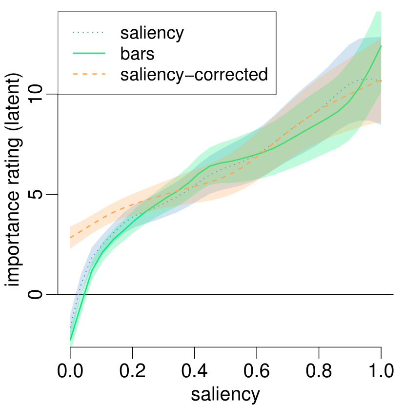
(a) Saliency score

(b) Word length

(c) Temporal display index

(d) Sentence length

(e) Word frequency

(f) Sentiment polarity

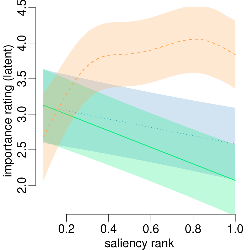
(g) Saliency rank

(h) Word position

Figure 11. Summed-effects comparison plots of the correction methods.

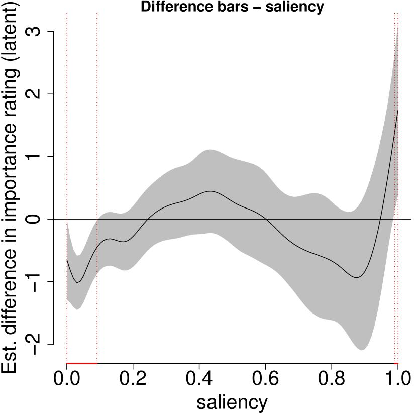
(a) Saliency score

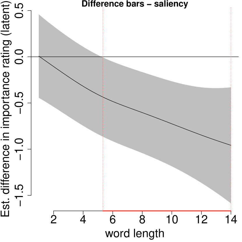
(b) Word length

(c) Temporal display index

(d) Sentence length

(e) Word frequency

(f) Sentiment polarity

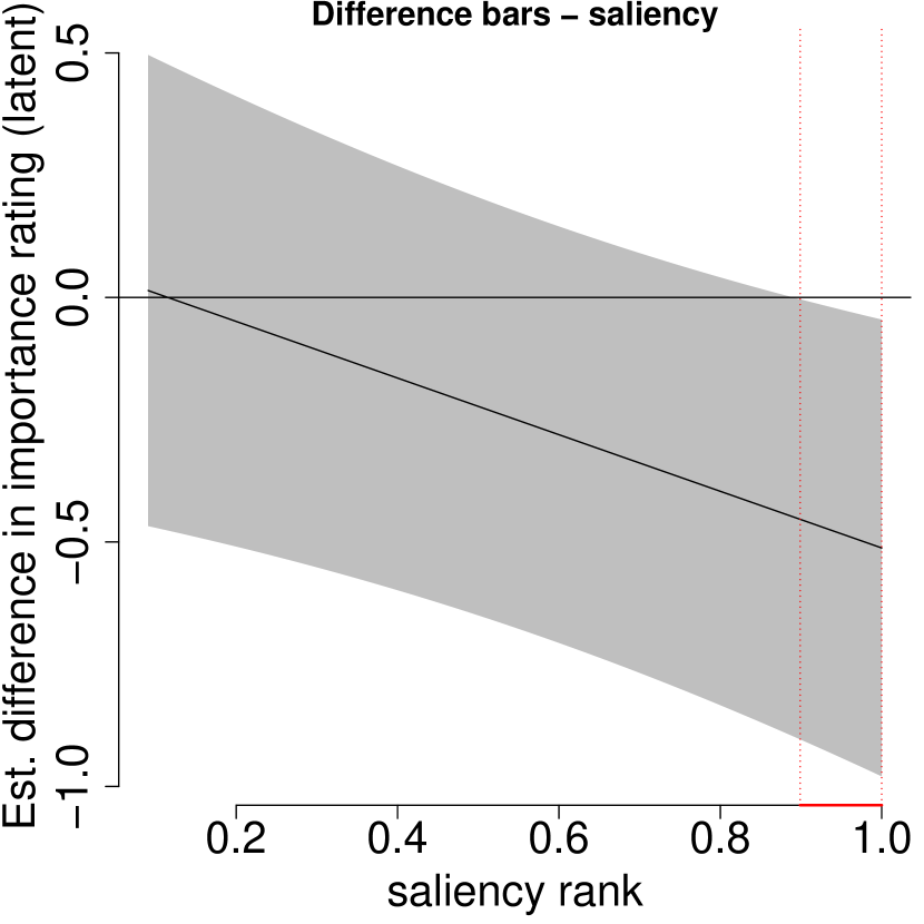
(g) Saliency rank

(h) Word position

Figure 12. Difference plots between the bar visualization and the original visualization. Areas of significant differences are marked red.

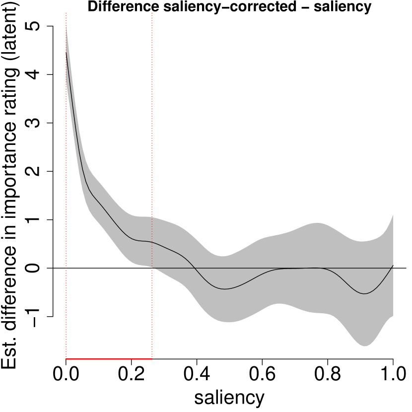
(a) Saliency score

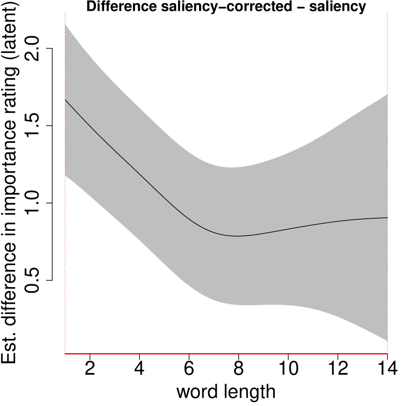
(b) Word length

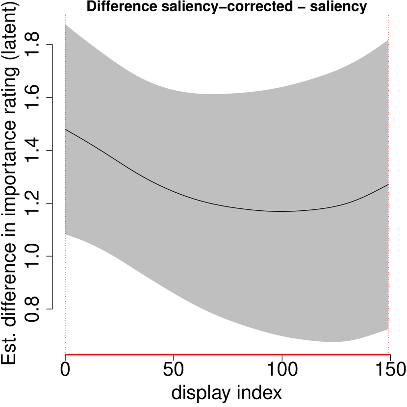
(c) Temporal display index

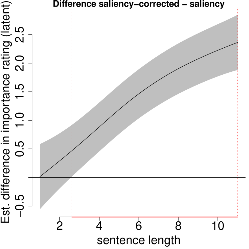
(d) Sentence length

(e) Word frequency

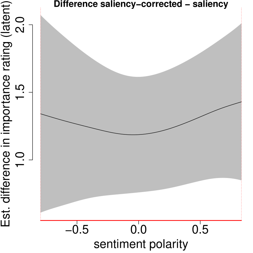
(f) Sentiment polarity

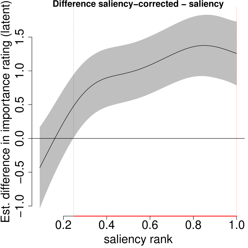
(g) Saliency rank

(h) Word position

Figure 13. Difference plots between the model-corrected saliencies and original saliencies. Areas of significant differences are marked red.