A semiparametric approach for interactive fixed effects panel data models

Abstract

This paper presents a new approach for the estimation and inference of the regression parameters in a panel data model with interactive fixed effects. It relies on the assumption that the factor loadings can be expressed as an unknown smooth function of the time average of covariates plus an idiosyncratic error term. Compared to existing approaches, our estimator has a simple partial least squares form and does neither require iterative procedures nor the previous estimation of factors. We derive its asymptotic properties by finding out that the limiting distribution has a discontinuity, depending on the explanatory power of our basis functions which is expressed by the variance of the error of the factor loadings. As a result, the usual “plug-in” methods based on estimates of the asymptotic covariance are only valid pointwise and may produce either over- or under-coverage probabilities. We show that uniformly valid inference can be achieved by using the cross-sectional bootstrap. A Monte Carlo study indicates good performance in terms of mean squared error. We apply our methodology to analyze the determinants of growth rates in OECD countries.

JEL classification: C01, C14, C33, C38.
Keywords: cross-sectional dependence, semiparametric factor models, principal components, sieve approximation, large panels.

1 Introduction

In the presence of unobserved heterogeneity, panel data models have proved to be useful tools in the estimation of regression parameters. Indeed, a large proportion of the literature on panel data models assumes that the unobserved heterogeneity is accounted for additive effects (i.e., individual and/or time-specific components that can be correlated with the explanatory variables) and independent observations in the cross-sectional dimension (see Arellano, (2003), Baltagi, (2015), Hsiao, (2014), and the references therein). However, because of the growing importance of individuals’ economic and social interconnections, economic agents are typically interdependent. It turns out that, as it has been shown in Phillips and Sul, (2003) or Hsiao and Tahmiscioglu, (2008) among others, if we ignore this dependence, standard panel data estimation techniques can lead to misleading inferences.

Recently, panel data models with interactive effects (or factor structure) have become one of the most popular and successful tools for handling cross-sectional dependence. The multiplicative specification of the unobserved heterogeneity is very useful since it contains the conventional additive effects as special cases but, at the same time, it is considerably more flexible since it allows for time-varying individual effects. In other words, the common time-specific effects $\mathbf{f}_{t}$, called common factors, can have a different impact on the individual-specific effects $\boldsymbol{\boldsymbol{\lambda}}_{i}$, called factor loadings. Further, from the empirical point of view, using interactive effects is more realistic since the unobserved components are allowed to exhibit an arbitrary degree of correlation with the explanatory variables. This situation is quite common in economics and other social sciences where some of the regressors are decision variables that are affected by the unobserved heterogeneity. For instance, macroeconomic models use the interactive effects to capture aggregate shocks which might have heterogeneous impacts on the agents (see Bernanke et al., (2005) for example); microeconomic models (e.g. Carneiro et al., (2003)) use the factor structure to study individuals’ education decisions. In finance, Ross, (1976) and Fama and French, (1993), among others, use the factor structure to capture the unobserved heterogeneity in a more flexible way for asset pricing, whereas Stock and Watson, (2002), Bai and Ng, (2006), and Fan et al., (2021) use it for forecasting.

While the specification with interactive fixed effects is more realistic and flexible, consistent estimation of the parameters of interest becomes more complicated due to the non-existence of simple linear transformations to remove the fixed effects as in the additive case.

Several alternative estimation approaches have been developed (see Fan and Liao, (2021) and the references therein for an intensive review). For panels with a large cross-sectional dimension, $N$, but fixed time dimension, $T$, in order to remove the factor loadings, in Holtz-Eakin et al., (1988) it is proposed a quasi-differencing transformation of the original model that treats $\mathbf{f}_{t}$ as a fixed number of parameters that need to be estimated. However, if there are too many parameters to estimate the incidental parameters problem may arise, see Neyman and Scott, (1948). To overcome it, in Ahn et al., (2001, 2013) consistent estimators of the parameters of interest are obtained through Generalized Method of Moments by imposing second-moment restrictions on the factor loadings.

More recent literature considers panels with both large $N$ and $T$. In order to obtain consistent estimators of the slope parameters, $\boldsymbol{\beta}$, the two most common approaches to deal with the interactive effects are the so-called common correlated effects (CCE) approach of Pesaran, (2006), and the principal components approach (PCA) of Bai, (2009). In general, both procedures are based on a two-stage strategy. The unknown common factors are estimated in the first step and then, the parameters of interest are estimated conditionally on the first-step factors estimates. However, both approaches exhibit relevant differences. On the one hand, in Pesaran, (2006) it is proposed to augment the original model with the cross-sectional averages of both the dependent variable, $y_{it}$, and a vector of explanatory variables, $\mathbf{X}_{it}$. These augmented variables are employed to control for the interactive fixed effects. On the other hand, in Bai, (2009) it is proposed an iterative estimation procedure where OLS residuals from a regression model that ignores the interactive effects are used to compute pilot estimates of common factors. These estimates are used to compute a partial least squares estimator of the slope parameters and then iterate until convergence. Alternatively, in Greenaway-McGrevy et al., (2012) it is proposed to augment the panel regression with some other factor estimates from $\mathbf{X}_{it}$. Recently, in Beyhum and Gautier, (2022), the dependence between regressors and the unobserved factors are modeled through a fully parametric factor structure. For other recent accounts on the estimation of interactive fixed effects models, see Ando and Bai, (2017), Bai and Li, (2014), Li et al., (2016), Moon and Weidner, (2015), Moon and Weidner, (2017), Peng et al., (2021), Chen et al., (2021), and Su et al., (2012), among others.

In this paper, we propose a novel semiparametric approach to estimate the regression parameters in a panel data model with interactive fixed effects. The basic idea is to extend the projected-PCA approach, originally proposed in Fan et al., (2016), for a pure factor model, to a panel data model with interactive fixed effects. More precisely, we assume the existence of a nonparametric relationship between factor loadings and the time average of covariates. By incorporating this information into the model of interest, the regression model takes the form of a partially linear model (see, e.g. Härdle et al., (2012)) and a new estimation approach can be proposed based on partialling out the interactive effects by using the sieve basis functions. Unlike the aforementioned literature, the estimation procedure proposed in this paper is very appealing for several reasons that can be summarized as the following:

• The resulting estimator for the slope parameter relies on a convex OLS problem which avoids iterative procedures that can be computationally intensive as the one proposed in Bai, (2009).

• Since we do not need to estimate the latent factors in a first step (as is the case in Bai, (2009)), the resulting estimator for the slope parameter is unaffected by the number of latent factors and does not require knowledge of them. This is a very interesting feature since the incidental parameter problem that usually characterized this type of model is avoided for $T$ fixed or large (see Bai, (2009) for further details).

• The underlying limiting distribution of the resulting estimator for the slope parameter is centered at zero. Therefore, it is proved that the proposed estimation technique enables us to circumvent omitted variable bias terms similar to the obtained in Bai, (2009) in the case of heteroskedastic and correlated error terms.

• Extending the Mundlak-Chamberlain projection approach (see Mundlak, (1978) and Chamberlain, (1984)), our proposal avoids misspecification problems that might arise from the standard linear relationship that relates factor loadings and time averages of regressors.

Under rather weak conditions the asymptotic properties of the proposed estimator for the slope parameter are obtained. Note that these asymptotic results hold irrespectively of the variance of the idiosyncratic part of the factor loadings being zero, close to zero, or much larger than zero. However, there exists a discontinuity in the limiting distribution of the estimator of the slope parameters when this variance is close to zero. This makes the standard “plug-in” inference tools, estimating the asymptotic covariance of the slope parameters, only valid pointwise and may produce biased coverage probabilities. We solve this problem by using a cross-sectional bootstrap procedure. By sampling the whole time es of the cross-sectional units, we are able to mimic the asymptotic distribution, and we can conduct uniformly valid inferences. Finally, under the condition that the loadings can be fully explained by the nonparametric functions, it is shown that our estimator reaches the semiparametric efficiency bound.

We validate the theoretical results in a simulation study. In the case where the time averages of regressors have a non-vanishing explanatory power on the factor loadings, our estimator outperforms alternative estimators which do not account for the relation. Later, we apply our method to the identification of the determinants of economic growth. Lu and Su, (2016) argued that the GDP growth rates per capita might not only be determined by observed factors but might also be influenced by latent factors or shocks. Our projection-based interactive fixed effects estimator is well suited for such a setting. Indeed, our empirical findings suggest an important role in these latent effects.

The rest of the paper is organized as follows. In Section 2, we present the model setup and derive our projection-based interactive fixed effects estimator. Also, consistent estimators for the latent factors and corresponding factor loadings are provided. Section 3 states our assumptions and studies the asymptotic properties of the proposed estimators. Based on these results, a consistent estimator of the standard errors of the estimated parameters is also provided. In Section 4, we examine the performance of our estimator in a Monte Carlo study. We apply our method to analyze the determinants of economic growth in Section 5. Section 6 concludes. All proofs are provided in the Appendix.

2 Model and Estimation Procedure

Let us consider the following panel data model with interactive fixed effects,

$$\begin{array}[]{ll}y_{it}&=\mathbf{X}_{it}^{\top}\boldsymbol{\boldsymbol{\beta}}+v_{it},\\ v_{it}&=\boldsymbol{\boldsymbol{\lambda}}_{i}^{\top}\mathbf{f}_{t}+u_{it}\end{array}\qquad i=1,\ldots,N;\quad t=1,\ldots,T,$$ (3)

where $y_{it}$ denotes the response variable of the individual $i$ in period $t$, $\mathbf{X}_{it}$ is the $Q$-dimensional covariate vector, $\boldsymbol{\boldsymbol{\beta}}$ is the $Q$-dimensional vector of parameters to be estimated, and $v_{it}$ has a factor structure. More precisely, the relationship between $\mathbf{X}_{it}$ and $y_{it}$ described in (3) contains $K$ common factors, $\mathbf{f}_{t}=(f_{t1},\ldots,f_{tK})^{\top}$, and the corresponding factor loadings for individual $i$, $\boldsymbol{\boldsymbol{\lambda}}_{i}^{\top}=(\lambda_{i1},\ldots,\lambda_{iK})$, so that $\boldsymbol{\boldsymbol{\lambda}}_{i}^{\top}\mathbf{f}_{t}=\lambda_{i1}f_{t1}+\ldots+\lambda_{iK}f_{tK}$. Further, these quantities are perturbed by the idiosyncratic error term, $u_{it}$, which is assumed to be independent of the regressors and the interactive effect components. Throughout the paper, $\boldsymbol{\boldsymbol{\lambda}}_{i}$, $\mathbf{f}_{t}$, and $u_{it}$ are all unobserved, and the dimension $K$ of the factor loadings does not depend on the cross-section size $N$ or the time series length $T$. This interactive effects setting generalizes the usual additive individual and time effects. For example, if $\boldsymbol{\boldsymbol{\lambda}}_{i}\equiv 1$, then $\boldsymbol{\boldsymbol{\lambda}}_{i}^{\top}\mathbf{f}_{t}=\mathbf{f}_{t}$, whereas if $\mathbf{f}_{t}\equiv 1$ we get $\boldsymbol{\boldsymbol{\lambda}}_{i}^{\top}\mathbf{f}_{t}=\boldsymbol{\boldsymbol{\lambda}}_{i}$.

2.1 Semiparametric Interactive Fixed Effects Model

Our interest is focused on the estimation of the slope coefficient vector, $\boldsymbol{\boldsymbol{\beta}}$. Nevertheless, in most of the empirical studies, some of the regressors, $\mathbf{X}_{it}$, are decision variables that are influenced by the unobserved individual heterogeneities, $\boldsymbol{\boldsymbol{\lambda}}_{i}$. Therefore, any attempt to estimate the slope parameters, $\boldsymbol{\boldsymbol{\beta}}$, directly through standard panel data estimation techniques will lead to inconsistent estimators. This is because standard panel data transformations (i.e., within or first differences transformation) are unable to remove the unobserved heterogeneities from the statistical model given the multiplicative form of these terms.

To avoid the more than likely omitted variable bias, one method is to control the dependence between the regressors and factor terms using the Mundlak-Chamberlain projection and incorporate this information into the model of interest. More precisely, as noted in Bai, (2009), when $\boldsymbol{\boldsymbol{\lambda}}_{i}$ is correlated with the regressors, it can be projected onto the regressors such that

$$\boldsymbol{\boldsymbol{\lambda}}_{i}=\boldsymbol{\psi}\mathbf{\bar{X}}_{i\cdot}+\boldsymbol{\boldsymbol{\gamma}}_{i},\quad i=1,\cdots,N,$$ (4)

where $\mathbf{\bar{X}}_{i\cdot}=T^{-1}\sum^{T}_{t=1}\mathbf{X}_{it}$, $\boldsymbol{\psi}$ is a $K\times Q$ matrix of unknown parameters, and $\boldsymbol{\boldsymbol{\gamma}}_{i}$ is a $K\times 1$ idiosyncratic component of the loading coefficients that cannot be explained by the covariates $\mathbf{\bar{X}}_{i\cdot}$ (i.e., the projection residuals).

However, the previous approach presents some drawbacks. In fact, there is a high degree of uncertainty surrounding the way in which the regressors may affect the factor loadings. Indeed there can be several situations in which tight functional specifications such as (4) can lead to inconsistent estimators and misleading inferences. To deal with this potential functional misspecification, we propose an alternative nonparametric specification to control the dependence between $\mathbf{X}_{it}$ and $\boldsymbol{\boldsymbol{\lambda}}_{i}$ in a more flexible way and we assume that this dependence can be modeled as

$$\boldsymbol{\boldsymbol{\lambda}}_{i}=\mathbf{g}(\mathbf{\bar{X}}_{i\cdot})+\boldsymbol{\boldsymbol{\gamma}}_{i},\quad i=1,\cdots,N,$$ (5)

where $\mathbf{g}(\mathbf{\bar{X}}_{i\cdot})=(g_{1}(\mathbf{\bar{X}}_{i\cdot}),\ldots,g_{K}(\mathbf{\bar{X}}_{i\cdot}))^{\top}$ is a $K\times 1$ vector of unknown functions and $\{\boldsymbol{\boldsymbol{\gamma}}_{i}\}_{i\leq N}$ is an error term. Plugging (5) into (3) and rearranging terms, we get

$$y_{it}=\mathbf{X}_{it}^{\top}\boldsymbol{\boldsymbol{\beta}}+\mathbf{g}(\mathbf{\bar{X}}_{i\cdot})^{\top}\mathbf{f}_{t}+\boldsymbol{\boldsymbol{\gamma}}_{i}^{\top}\mathbf{f}_{t}+u_{it}.$$ (6)

Model (6) reduces to model (3) when $\mathbf{g}(\cdot)=0$ and furthermore, if $\boldsymbol{\beta}=0$ it reduces to the model proposed in Fan et al., (2016). Finally, if $\mathbf{g}(\cdot)\neq 0$, $\gamma_{ik}=0$ and $\boldsymbol{\beta}=0$, model (6) reduces to the semiparametric factor model proposed in Connor and Linton, (2007) and Connor et al., (2012).

It is worth noting that ignoring $\boldsymbol{\lambda}^{\top}_{i}\boldsymbol{f}_{t}$ in the presence of (5) results still in a nontrivial omitted variable bias problem for the OLS estimators of the $\boldsymbol{\beta}$’s. More interestingly, this problem persists even imposing conditions of the type $\mathop{\mbox{\sf E}}\left(f{X}_{it}{\boldsymbol{\gamma}}^{\top}_{i}\mathbf{f}_{t}\right)=0$. In this case, we would obtain that $\mathop{\mbox{\sf E}}(\mathbf{X}_{it}\mathbf{g}(\mathbf{\bar{X}}_{i.})^{\top}\mathbf{f}_{t})\neq 0$ and therefore direct OLS estimators of $\boldsymbol{\beta}$ will be still biased.

Model (6) can be written in matrix form as

$$\mathbf{y}_{t}=\mathbf{X}_{t}\boldsymbol{\beta}+\mathbf{G}(\mathbf{\bar{X}})\mathbf{f}_{t}+v_{t},\qquad t=1,\ldots,T,$$ (7)

where $\mathbf{y}_{t}$ and $v_{t}$ are $N\times 1$ vectors of $y_{it}$ and $v_{it}$, respectively, $\mathbf{X}_{t}$ is a $N\times Q$ matrix of regressors, $\mathbf{G}(\mathbf{\bar{X}})$ is a $N\times K$ matrix of unknown functions, $g_{k}(\mathbf{\bar{X}}_{i\cdot})$, and finally $\mathbf{v}_{t}=\boldsymbol{\Gamma}\mathbf{f}_{t}+\mathbf{u}_{t}$, where $\boldsymbol{\Gamma}=(\boldsymbol{\gamma}_{1},\ldots,\boldsymbol{\gamma}_{N})^{\top}$ is a $N\times K$ matrix of unknown loading coefficients and $\mathbf{u}_{t}=\left(u_{1t},\cdots,u_{Nt}\right)^{\top}$ is a $N\times 1$ vector of idiosyncratic errors.

In this framework, in order to obtain a consistent estimator for $\boldsymbol{\beta}$, and assuming that the inverses are properly defined, we propose to partial the term $\mathbf{G}\left(\mathbf{\bar{X}}\right)\mathbf{f}_{t}$ out from (7). If we do this we will obtain the following expression

$$\boldsymbol{\boldsymbol{\widehat{\boldsymbol{\beta}}}}_{G} = \left\{\sum_{t=1}^{T}\mathbf{X}^{\top}_{t}\left[\mathbf{I}_{N}-\mathbf{P}\left(\mathbf{\bar{X}}\right)\right]\mathbf{X}_{t}\right\}^{-1}\sum_{t=1}^{T}\mathbf{X}_{t}^{\top}\left[\mathbf{I}_{N}-\mathbf{P}\left(\mathbf{\bar{X}}\right)\right]\mathbf{y}_{t},$$ (8)

where

$$\mathbf{P}\left(\mathbf{\bar{X}}\right)=\mathbf{G}(\mathbf{\bar{X}})\left[\mathbf{G}(\mathbf{\bar{X}})^{\top}\mathbf{G}(\mathbf{\bar{X}})\right]^{-1}\mathbf{G}(\mathbf{\bar{X}})^{\top}.$$ (9)

Unfortunately the computation of $\boldsymbol{\boldsymbol{\widehat{\boldsymbol{\beta}}}}_{G}$ is unfeasible because the matrix of nonparametric functions, $\mathbf{G}(\mathbf{\bar{X}})$, is unknown to the practitioner. In order to solve this problem we propose to estimate $\mathbf{G}(\mathbf{\bar{X}})$ by the sieve method. To estimate nonparametrically $g_{k}(\cdot)$ without the curse of dimensionality when $Q$ is large, it will be assumed that for each $k$, where $k=1,\ldots,K$, $g_{k}(\cdot)$ is an additive function of the form

$$g_{k}\left(\mathbf{\bar{X}}_{i.}\right)=\sum^{Q}_{q=1}g_{kq}\left(\bar{X}_{i.,q}\right),\quad i=1,\ldots,N,\quad q=1,\ldots,Q.$$ (10)

For each $k$ and $q$, each additive component $g_{kq}(\cdot)$ can be approximated by the sieve method. If we define $\left\{\phi_{1}(\bar{X}_{i\cdot,q}),\cdots,\phi_{J}(\bar{X}_{i\cdot,q})\right\}$ as a set of basis functions (i.e., splines, Fourier series, wavelets), which spans a dense linear space of the functional space for $g_{kq}$. Then

$$g_{kq}(\bar{X}_{i\cdot,q})=\sum_{\ell=1}^{J}b_{\ell,kq}\phi_{\ell}(\bar{X}_{i\cdot,q})+R_{kq}(\bar{X}_{i\cdot,q}),\quad k=1,\ldots,K,\quad q=1,\ldots,Q,$$ (11)

where, for $\ell=1,\ldots,J$, $\phi_{\ell}(\cdot)$’s are the sieve basis functions, $b_{\ell,kq}$’s are the sieve coefficients of the $q$th additive component of $g_{k}(\mathbf{\bar{X}}_{i\cdot})$ corresponding to the $k$th factor loading, $R_{kq}(\cdot)$ is a “remainder function” that represents the approximation error, and $J$ denotes the number of sieve terms which grows slowly as $N\rightarrow\infty$. As it is well known in the literature, the approximation functions $\phi_{\ell}(\cdot)$ have the property that, as $J$ grows, there is a linear combination of $\phi_{\ell}(\cdot)$ that can approximate any smooth function $g_{k}(\cdot)$ arbitrarily well in the sense that the approximation error can be made arbitrarily small. Therefore, the basic assumption for sieve approximation is that $\sup_{x}|R_{kq}(x)|\rightarrow 0$, as $J\rightarrow\infty$. In practice, an optimal choice for the smoothing parameter $J$ can be based on cross-validation.

For the sake of simplicity, we take the same basis functions in (11) and, for each $k\leq K$, $q\leq Q$ and $i\leq N$, let us define

$$\mathbf{b}_{k}^{\top} =(b_{1,k1},\ldots,b_{J,k1},\ldots,b_{1,kQ},\ldots,b_{J,kQ})\in\mathbb{R}^{JQ},$$

$$\phi(\mathbf{\bar{X}}_{i\cdot})^{\top} =(\phi_{1}(\bar{X}_{i\cdot,1}),\ldots,\phi_{J}(\bar{X}_{i\cdot,1}),\ldots,\phi_{1}(\bar{X}_{i\cdot,Q}),\ldots,\phi_{J}(\bar{X}_{i\cdot,Q}))\in\mathbb{R}^{JQ},$$

so the above equation can be rewritten as

$$g_{k}(\mathbf{\bar{X}}_{i\cdot})=\phi(\mathbf{\bar{X}}_{i\cdot})^{\top}\mathbf{b}_{k}+\sum^{Q}_{q=1}R_{kq}(\mathbf{\bar{X}}_{i\cdot,q}).$$ (12)

Let $\Phi(\mathbf{\bar{X}})=(\phi(\mathbf{\bar{X}}_{1\cdot}),\ldots,\phi(\mathbf{\bar{X}}_{N\cdot}))^{\top}$ be a $N\times JQ$ matrix of basis functions, $\mathbf{B}=(\mathbf{b}_{1},\ldots,\mathbf{b}_{K})$ be a $JQ\times K$ matrix of sieve coefficients, and $\mathbf{R}(\mathbf{\bar{X}})$ be a $N\times K$ matrix with the $(i,k)$th element $\sum^{Q}_{q=1}R_{kq}(\mathbf{\bar{X}}_{i\cdot,q})$. By considering (12) in matrix form, we obtain

$$\mathbf{G}(\mathbf{\bar{X}})=\Phi(\mathbf{\bar{X}})\mathbf{B}+\mathbf{R}(\mathbf{\bar{X}})$$ (13)

and substituting (13) into (7) it leads to

$$\mathbf{y}_{t}=\mathbf{X}_{t}\boldsymbol{\beta}+\Phi(\mathbf{\bar{X}})\mathbf{B}\mathbf{f}_{t}+\mathbf{R}(\mathbf{\bar{X}})\mathbf{f}_{t}+\mathbf{v}_{t},\qquad t=1,\ldots,T,$$ (14)

where it can be noted that the residual term consists of two parts: the sieve approximation error, $\mathbf{\bar{X}})\mathbf{f}_{t}$, and the error term, $\mathbf{v}_{t}$. Assuming the inverse is properly defined, we will replace $\mathbf{P}(\mathbf{\bar{X}})$ in (9) by

$$\mathbf{P}_{\Phi}(\mathbf{\bar{X}})=\Phi(\mathbf{\bar{X}})\left[\Phi(\mathbf{\bar{X}})^{\top}\Phi(\mathbf{\bar{X}})\right]^{-1}\Phi(\mathbf{\bar{X}})^{\top},$$ (15)

In this situation, instead of projecting on the space of factors $\mathbf{f}_{t}$, we consider a sieve estimation for $\mathbf{G}(\mathbf{\bar{X}})$ to estimate $\boldsymbol{\beta}$ and project on the space expanded by the sieve basis. Therefore, this approach has the advantage that we are able to estimate the slope parameter directly circumventing the necessity to estimate the latent factors in a first step.

Therefore, one can obtain the estimator of $\boldsymbol{\beta}$ by partialling out the nonparametric part of the factor loadings, i.e.,

$$\boldsymbol{\boldsymbol{\widehat{\boldsymbol{\beta}}}}=\left\{\sum_{t=1}^{T}\mathbf{X}_{t}^{\top}\left[\mathbf{I}_{N}-\mathbf{P}_{\Phi}(\mathbf{\bar{X}})\right]\mathbf{X}_{t}\right\}^{-1}\sum_{t=1}^{T}\mathbf{X}_{t}^{\top}\left[\mathbf{I}_{N}-\mathbf{P}_{\Phi}(\mathbf{\bar{X}})\right]\mathbf{y}_{t},$$ (16)

where $\sum_{t=1}^{T}\mathbf{X}_{t}^{\top}\left[\mathbf{I}_{N}-\mathbf{P}_{\Phi}(\mathbf{\bar{X}})\right]\mathbf{X}_{t}$ is assumed to be asymptotically nonsingular. It is worth noting that the resulting estimator of $\boldsymbol{\beta}$ appears as the solution of a partially linear model (see Härdle et al., (2012) for a comprehensive review of the literature), where the nonparametric part is “partialled out”.

2.2 Estimation of Factors and Loadings

In this subsection, we show how to estimate the factors and the loadings once we have available an estimate for the slope parameters. Note however that for the estimation of $\boldsymbol{\beta}$, as it has been already pointed out, it is not necessary to estimate previously $\mathbf{f}_{t}$ or $\boldsymbol{\boldsymbol{\lambda}}_{i}$. To estimate the latent factors and corresponding factor loadings we propose to use the projected PCA approach proposed in Fan et al., (2016) in a slightly different context. More precisely, owing to potential correlations between the unobservable effects and the regressors, we treat the matrix of common factors $\mathbf{F}=(\mathbf{f}_{1},\ldots,\mathbf{f}_{T})^{\top}$ as fixed-effects parameters to be estimated. The latent factors and corresponding factor loadings can be estimated from the regression residuals, $\mathbf{\widetilde{y}}_{t}=\mathbf{y}_{t}-\mathbf{X}_{t}\boldsymbol{\boldsymbol{\widehat{\boldsymbol{\beta}}}}$, and let $\mathbf{\widetilde{Y}}=(\mathbf{\widetilde{y}}_{1},\ldots,\mathbf{\widetilde{y}}_{T})$. Now $\mathbf{F}$ and $\mathbf{G}(\bar{X})$ can be recovered from the projected data $\mathbf{P}_{\Phi}(\mathbf{\bar{X}})\mathbf{\widetilde{Y}}$ under the following identification restrictions: (i) $T^{-1}\mathbf{F}^{\top}\mathbf{F}=I_{K}$ and (ii) $\mathbf{G}(\mathbf{\bar{X}})^{\top}\mathbf{G}(\mathbf{\bar{X}})$ is a $K\times K$ diagonal matrix with distinct entries. Then, $\sqrt{T}\mathbf{\widehat{F}}$ can be estimated by the eigenvectors associated with the largest $K$ eigenvalues of the matrix $T^{-1}\mathbf{\widetilde{Y}}^{\top}\mathbf{P}_{\Phi}(\mathbf{\bar{X}})\mathbf{\widetilde{Y}}$.

Once we estimated $\mathbf{\widehat{F}}$, it is possible to obtain an estimator for the sieve coefficients using a least squares procedure that leads to

$$\mathbf{\widehat{B}}=(\mathbf{\widehat{b}}_{1},\ldots,\mathbf{\widehat{b}}_{K})=\frac{1}{T}\left[\Phi(\mathbf{\bar{X}})^{\top}\Phi(\mathbf{\bar{X}})\right]^{-1}\Phi(\mathbf{\bar{X}})^{\top}\mathbf{\widetilde{Y}}\mathbf{\widehat{F}},$$ (17)

and replacing (17) into (12), we can construct an estimator for the nonparametric functions $g_{k}(\cdot)$ of the form

$$\widehat{g}_{k}(x)=\phi(x)^{\top}\mathbf{\widehat{b}}_{k},\quad k=1,\ldots,K.$$ (18)

Let $\boldsymbol{\boldsymbol{\Lambda}}$ be the $N\times K$ matrix of factor loadings, then we can estimate $\boldsymbol{\widehat{\boldsymbol{\Lambda}}}=\mathbf{\widetilde{Y}}\mathbf{\widehat{F}}/T$ (see Fan et al., (2016) for further details). Therefore, the part of the factor loadings in (5) that can be explained by $\mathbf{\bar{X}}$ can be estimated by $\mathbf{\widehat{G}}(\mathbf{\bar{X}})=\frac{1}{T}\mathbf{P}_{\Phi}(\mathbf{\bar{X}})\mathbf{\widetilde{Y}}\mathbf{\widehat{F}}$, whereas the idiosyncratic part can be calculated as $\boldsymbol{\widehat{\boldsymbol{\Gamma}}}=\boldsymbol{\widehat{\boldsymbol{\Lambda}}}-\mathbf{\widehat{G}}(\mathbf{\overline{X}})=\frac{1}{T}[\mathbf{I}_{N}-\mathbf{P}_{\Phi}(\mathbf{\bar{X}})]\mathbf{\widetilde{Y}}\mathbf{\widehat{F}}$.

Finally, note that the number of latent factors, $K$, is unknown but can be estimated from the data. We follow the approach of Fan et al., (2016) to select $\widehat{K}$ according to the largest ratio of eigenvalues of the matrix $\mathbf{\widetilde{Y}}^{\top}\mathbf{P}_{\Phi}(\mathbf{\bar{X}})\mathbf{\widetilde{Y}}$,

$$\widehat{K}=\arg\max_{0<k<J_{g}Q/2}\frac{\lambda_{k}\left[\mathbf{\widetilde{Y}}^{\top}\mathbf{P}_{\Phi}(\mathbf{\bar{X}})\mathbf{\widetilde{Y}}\right]}{\lambda_{k+1}\left[\mathbf{\widetilde{Y}}^{\top}\mathbf{P}_{\Phi}(\mathbf{\bar{X}})\mathbf{\widetilde{Y}}\right]},$$ (19)

where $\lambda_{k}[\mathbf{\widetilde{Y}}^{\top}\mathbf{P}_{\Phi}(\mathbf{\bar{X}})\mathbf{\widetilde{Y}}]$ denotes the $k$-largest eigenvalue of the matrix.

Note that the condition on the true number of factors, i.e., $0<K<JQ/2$ in (19), is fulfilled naturally since the sieve dimension $J$ grows slowly with the sample size. Interestingly, our estimator for the regression parameters, $\boldsymbol{\boldsymbol{\widehat{\boldsymbol{\beta}}}}$, does not require any knowledge of $K$. However, the number of factors is crucial to the estimation of the factor components as well as to the estimation of standard errors for the regression parameters.

3 Asymptotic Properties

In this section, we analyze the main asymptotic properties of the proposed estimators. Firstly, we introduce some notation, definitions, and assumptions that will be necessary to derive the main results of this paper. Later, we present the main large sample properties of these estimators.

3.1 Notation

Let $n=NT$. For two positive number sequences $(a_{n})$ and $(b_{n})$, we say $a_{n}={\mathcal{O}}(b_{n})$ or $a_{n}\lesssim b_{n}$ (resp. $a_{n}\asymp b_{n}$) if there exists $C>0$ such that $a_{n}/b_{n}\leq C$ (resp. $1/C\leq a_{n}/b_{n}\leq C$) for all large $n$, and say $a_{n}={\scriptstyle{\mathcal{O}}}(b_{n})$ if $a_{n}/b_{n}\rightarrow 0$ as $n\rightarrow\infty$. We set $(X_{n})$ and $(Y_{n})$ to be two sequences of random variables. Write $X_{n}={\mathcal{O}}_{p}(Y_{n})$ if for $\forall\epsilon>0$, there exists $C>0$ such that $\mathrm{P}(X_{n}/Y_{n}\leq C)>1-\epsilon$ for all large $n$, and say $X_{n}={\scriptstyle{\mathcal{O}}}_{p}(Y_{n})$ if $X_{n}/Y_{n}\rightarrow 0$ in probability as $n\rightarrow\infty$. Through this paper, for a real matrix $\mathbf{A}$, let $\|\mathbf{A}\|_{F}={\rm tr}^{1/2}(\mathbf{A}^{\top}\mathbf{A})$ and $\|\mathbf{A}\|_{2}=\lambda_{\max}^{1/2}(\mathbf{A}^{\top}\mathbf{A})$ denote its Frobenius and spectral norms, respectively. Let $\lambda_{\min}(\cdot)$ and $\lambda_{\max}(\cdot)$ denote the minimum and maximum eigenvalues of a square matrix. For a vector v, let $\|\textbf{v}\|$ denote its Euclidean norm.

3.2 Definitions and Assumptions

DEFINITION 3.1

A function $h(\cdot)$ is said to belong to a Hölder class of functions $\mathcal{G}$, if $\forall q\leq Q$ and $k\leq K$, $h(\cdot)$ belongs to

$$\left\{h:|h^{(r)}(s)-h^{(r)}(t)|\leq L|s-t|^{\alpha}\right\}$$

for some $L>0$, and for all $s$ and $t$ in the domain of $h(\cdot)$, where $r$ is the degree of smoothing of the real-valued function $h(\cdot)$ and $0<\alpha\leq 1$.

For any scalar or vector function $\varphi(x)$, we use the notation $\Pi_{\mathcal{G}}[\varphi(x)]$ to denote the projection of $\varphi(x)$ onto the class of functions $\mathcal{G}$. That is, $\Pi_{\mathcal{G}}[\varphi(x)]$ is an element that belongs to $\mathcal{G}$ and it is the closest function to $\varphi(x)$ among all the functions in $\mathcal{G}$. More specifically, we have

$$\mathop{\mbox{\sf E}}\{[\varphi(x)-{\Pi}_{\mathcal{G}}(\varphi(x))][\varphi(x)-{\Pi}_{\mathcal{G}}(\varphi(x))]^{\top}\}$$

$$= \inf_{h\in\mathcal{G}}\mathop{\mbox{\sf E}}\{[\varphi(x)-h(x)][\varphi(x)-h(x)]^{\top}\},$$ (20)

where the infimum is in the sense that

$$\mathop{\mbox{\sf E}}\{[\varphi(x)-{\Pi}_{\mathcal{G}}(\varphi(x))][\pi(x)-{\Pi}_{\mathcal{G}}(\varphi(x))]^{\top}\}$$

$$\leq \Pi\{[\varphi(x)-h(x)][\varphi(x)-h(x)]^{\top}\},$$ (21)

for all $h\in\mathcal{G}$, where for square matrices $\mathbf{A}$ and $\mathbf{B}$, $\mathbf{A}\leq\mathbf{B}$ means that $\mathbf{A}-\mathbf{B}$ is negative definite.

Now we characterize the large sample behavior of $\left\{\mathbf{X}_{it}\right\}_{i\leq N;t\leq T}$, and its functionals,

Assumption 3.1 (Asymptotic behavior of $\mathbf{\bar{X}}$)

(i)

$T^{-1}\sum_{t=1}^{T}\mathbf{X}_{it}=\mathbf{\ddot{X}}_{i}+O_{p}(T^{-1/2}),\quad i=1,\ldots,N$, as $T$ tends to infinity, where $\mathbf{\ddot{X}}_{i}=(\ddot{X}_{i1},\ldots,\ddot{X}_{iQ})^{\top}$ is a $Q\times 1$ vector of random variables with support $\mathcal{X}_{i}$.

(ii)

Let $\mathbf{\ddot{X}}=\left(\mathbf{\ddot{X}}^{\top}_{1},\cdots,\mathbf{\ddot{X}}^{\top}_{N}\right)$ a $N\times Q$ matrix and denote by $\mathbf{\mathcal{X}}$ its support. For any $x\in\mathbf{\mathcal{X}}$ we assume that $\sup_{x\in\mathbf{\mathcal{X}}}\mathop{\mbox{\sf E}}\left(\left.\mathbf{X}_{t}\mathbf{X}^{\top}_{t}\right|\mathbf{\ddot{X}}=x\right)<C_{1}$, for some $C_{1}>0$.

(iii)

Let us define $\theta(\mathbf{\ddot{X}})=\mathop{\mbox{\sf E}}(\mathbf{X}_{t}|\mathbf{\ddot{X}})$ and $m(\mathbf{\ddot{X}})=\Pi_{\mathcal{G}}[\theta(\mathbf{\ddot{X}})]$ as the projection of $\theta(\mathbf{\ddot{X}})$ onto $\mathcal{G}$. Define also $\boldsymbol{\xi}_{t}=\mathbf{X}_{t}-m(\mathbf{\ddot{X}})$ and $\boldsymbol{\eta}(\mathbf{\ddot{X}})=\theta(\mathbf{\ddot{X}})-m(\mathbf{\ddot{X}})$. Finally, let $\boldsymbol{\varepsilon}_{t}=\mathbf{X}_{t}-\theta(\mathbf{\ddot{X}})$. $\theta(\mathbf{\ddot{X}})$, $m(\mathbf{\ddot{X}})$ and hence $\boldsymbol{\eta}(\mathbf{\ddot{X}})$ are bounded functions in $\mathcal{X}$. For any $x\in\mathbf{\mathcal{X}}$, we assume that $\sup_{x\in\mathbf{\mathcal{X}}}\mathop{\mbox{\sf E}}\left(\left.\boldsymbol{\varepsilon}_{t}\boldsymbol{\varepsilon}^{\top}_{t}\right|\mathbf{\ddot{X}}=x\right)<C_{2}$, $\sup_{x\in\mathbf{\mathcal{X}}}\mathop{\mbox{\sf E}}\left(\left.\boldsymbol{\xi}_{t}\boldsymbol{\xi}^{\top}_{t}\right|\mathbf{\ddot{X}}=x\right)<C_{3}$, for some $C_{2},C_{3}>0$, where both $\boldsymbol{\varepsilon}_{t}$ and $\boldsymbol{\xi}_{t}$ are $N\times Q$ matrices.

(iv)

Define

$$\widetilde{V}_{\xi}=\operatorname{plim}_{N,T\rightarrow\infty}\frac{1}{NT}\sum_{t}\boldsymbol{\xi}^{\top}_{t}\boldsymbol{\xi}_{t}.$$

$\widetilde{V}_{\xi}$ is finite and positive definite.

Assumption 3.1 characterizes the asymptotic behavior of $\mathbf{\bar{X}}$, when both $N$ and $T$ tend to infinity. For fixed $T$ this assumption would not be necessary. This assumption is related to the inference problem raised in Fernández-Val et al., (2022), p. 14. In addition, the following conditions about the data generating process, the projected PCA approach, basis functions, factor loadings, and sieve approximation are required. Let $\mathbf{G}(\mathbf{\ddot{X}})$ be defined analogously to $\mathbf{G}(\mathbf{\bar{X}})$ with $\mathbf{\bar{X}}$ replaced by $\mathbf{\ddot{X}}$.

As the reader can see, $\mathbf{F}$ and $\mathbf{G}(\cdot)$ are not separately identified in (7) so we need the following identification assumption.

Assumption 3.2 (Identification)

Almost surely, $T^{-1}\mathbf{F}^{\top}\mathbf{F}=\mathbf{I}_{K}$ and $\mathbf{G}(\mathbf{\ddot{X}})^{\top}\mathbf{G}(\mathbf{\ddot{X}})$ is a $K\times K$ diagonal matrix with distinct entries.

The condition detailed above is commonly used in the estimation of factor models and corresponds to condition PC1 of Bai and Ng, (2013) in the case of unprojected data. In particular, it enables to identify separately the factors $\mathbf{F}$ and the part of the loadings explained by the covariates, $\mathbf{G}(\mathbf{\ddot{X}})$, from their product $\mathbf{G}(\mathbf{\ddot{X}})\mathbf{F}$. In the following, let $\Phi(\mathbf{\ddot{X}})$ be defined analogously to $\Phi(\mathbf{\bar{X}})$ with $\mathbf{\bar{X}}$ replaced by $\mathbf{\ddot{X}}$.

Assumption 3.3 (Sieve basis functions)

(i)

There are two positive constants, $c_{\min}^{\prime}$ and $c_{\max}^{\prime}$ such that, with probability approaching one (as $N\rightarrow\infty$),

$$c_{\min}^{\prime}<\lambda_{min}\left(N^{-1}\Phi(\mathbf{\ddot{X}})^{\top}\Phi(\mathbf{\ddot{X}})\right)<\lambda_{max}\left(N^{-1}\Phi(\mathbf{\ddot{X}})^{\top}\Phi(\mathbf{\ddot{X}})\right)<c_{\max}^{\prime}.$$

(ii)

$\max_{j\leq J,i\leq N,q\leq Q}\mathop{\mbox{\sf E}}[\phi^{(\ell)}_{j}(\ddot{X}_{iq})^{2}]<\infty$, for $\ell=0,1,2$;

Assumption 3.4 (Accuracy of sieve approximation)

(i)

$g(\cdot)\in\mathcal{G}$ and $m(\cdot)\in\mathcal{G}$.

(ii)

For $h(\cdot)=g(\cdot)$ or $h(\cdot)=m(\cdot)$, the sieve coefficients $\{b_{j,kq}\}^{J}_{j=1}$ satisfy, for $\kappa=2(r+\alpha)\geq 4$ as $J\rightarrow\infty$,

$$\sup_{x\in\mathcal{X}_{iq}}\left|h_{kq}(x)-\sum_{j=1}^{J}b_{j,kq}\phi_{j}(x)\right|^{2}=\mathcal{O}\left(J^{-\kappa}\right),$$

where $\mathcal{X}_{iq}$ is the support of the $q-th$ element of $\mathcal{X}_{i}$, for $q=1,\ldots,Q$, and $J$ is the sieve dimension.

(iii)

$\max_{j,k,q}b_{j,kq}^{2}<\infty$ and $\sqrt{NT}J^{-\kappa/2}\rightarrow 0$ as $N\rightarrow\infty$ and $T\rightarrow\infty$.

As it is remarked in Fan et al., (2016), Assumption 3.4 (ii) is satisfied by the use of common basis functions such as polynomial basis or B-splines. In particular, Lorentz, (1986) and Chen, (2007) show that (i) implies (ii) in this particular case. Assumption 3.4(iii) is similar to other assumptions used in similar literature such as in Ahmad et al., (2005).

In order to obtain the asymptotic bound of $\boldsymbol{\widehat{\beta}}$ there is no need to assume an i.i.d. for the $\gamma_{ik}$’s, in fact, cross-sectional week dependence as in Assumption 3.5(ii) is enough, whereas the $i.i.d.$ condition will only be required later for the Central Limit Theorem (CLT). Write $\boldsymbol{\boldsymbol{\gamma}}_{i}=(\gamma_{i1},\ldots,\gamma_{iK})^{\top}$, and

$$\nu_{N}=\max_{k\leq K}N^{-1}\sum_{i\leq N}{\sf Var}(\gamma_{ik}),$$

the following assumption is required

Assumption 3.5 (Error factor loadings)

(i)

$\{\boldsymbol{\boldsymbol{\gamma}}_{i}\}_{i\leq N}$ is an error term and it is assumed that $\mathop{\mbox{\sf E}}(\gamma_{ik}|\mathbf{f}_{1},\cdots,\mathbf{f}_{T})=0$ for $k=1,\cdots,K$ and $\boldsymbol{\gamma}_{i}$ is independent of $\mathbf{\ddot{X}}_{i}$, for $i=1,\cdots,N$.

(ii)

$\max_{k\leq K,i\leq N}\mathop{\mbox{\sf E}}\left[g^{(\ell)}_{k}(\mathbf{\ddot{X}}_{i})^{2}\right]<\infty$, for $\ell=0,1,2$. Also, $\nu_{N}<\infty$ and

$$max_{k\leq K,j\leq N}\sum_{i\leq N}|\mathop{\mbox{\sf E}}(\gamma_{ik}\gamma_{jk})|=\mathcal{O}(\nu_{N}).$$

(iii)

For some $\delta>2$,

$$\max_{i\leq N;k\leq K}\mathop{\mbox{\sf E}}\left|\gamma_{ik}\mathop{\mbox{\sf E}}\left(\left.\xi_{itq}f_{kt}\right|\boldsymbol{\Gamma}\right)\right|^{\delta}<\infty,\quad q=1,\cdots,Q.$$ (22)

Through the paper, some regularity conditions about weak dependence and stationarity are assumed on the factors and the idiosyncratic terms. In particular, following Fan et al., (2016) we impose the strong mixing condition. Let $\mathcal{F}_{-\infty}^{0}$ and $\mathcal{F}_{T}^{\infty}$ denote the $\sigma$-algebras generated by $\{(\boldsymbol{\xi}_{t},\mathbf{f}_{t},\mathbf{u}_{t}):t\leq 0\}$ and $\{(\boldsymbol{\xi}_{t},\mathbf{f}_{t},\mathbf{u}_{t}):t\geq T\}$, respectively. Define the mixing coefficient

$$\alpha(T)=\sup_{A\in\mathcal{F}_{-\infty}^{0},B\in\mathcal{F}_{T}^{\infty}}|\mathrm{P}(A)\mathrm{P}(B)-\mathrm{P}(AB)|.$$

Assumption 3.6 (Data generating process)

(i)

$\{\boldsymbol{\xi}_{t},\mathbf{u}_{t},\mathbf{f}_{t}\}_{t\leq T}$ is strictly stationary.

$\{\mathbf{u}_{t}\}_{t\leq T}$ is independent of $\{\mathbf{\ddot{X}}_{i},\boldsymbol{\xi}_{t},\mathbf{f}_{t}\}_{i\leq N;t\leq T}$.

In addition, $\mathop{\mbox{\sf E}}(u_{it})=0$ for all $i\leq N$, $t\leq T$.

(ii)

For some $\delta>2$,

$$\max_{t\leq T}\mathop{\mbox{\sf E}}\left|\xi_{itq}u_{it}\right|^{\delta}<\infty,\quad i=1,\cdots,N;\quad q=1,\cdots,Q.$$ (23)

(iii)

Strong mixing: $\alpha(k)=ak^{-\tau}$, where $a$ is a positive constant and $\tau>\frac{\delta}{\delta-2}$.

(iv)

Weak dependence: there is $C>0$ so that

$$\max_{j\leq N}\sum_{i=1}^{N}|\mathop{\mbox{\sf E}}(u_{it}u_{jt})| <C,$$

$$\frac{1}{NT}\sum_{i=1}^{N}\sum_{j=1}^{N}\sum_{t=1}^{T}\sum_{s=1}^{T}|\mathop{\mbox{\sf E}}(u_{it}u_{js})| <C,$$

$$\max_{i\leq N}\frac{1}{NT}\sum_{l=1}^{N}\sum_{l^{\prime}=1}^{N}\sum_{t=1}^{T}\sum_{s=1}^{T}\left|{\sf Cov}\left(u_{it}u_{lt},u_{is}u_{l^{\prime}s}\right)\right| <C.$$

(v)

Exponential tail: there exist $r_{2},r_{3}>0$ satisfying $r_{1}^{-1}+r_{2}^{-1}+r_{3}^{-1}>1$ and $b_{1},b_{2}>0$, such that for any $s>0$, $i\leq N$ and $\ell\leq J$,

$$\mathrm{P}\left(|u_{it}|>x\right)\leq\exp\left\{-\left(x/b_{1}\right)^{\alpha_{2}}\right\},$$

$$\mathrm{P}\left(|f_{kt}|>x\right)\leq\exp\left\{-\left(x/b_{2}\right)^{\alpha_{3}}\right\},$$

where $\alpha_{2}$ and $\alpha_{3}$ are two positive constants.

Assumption 3.6 is standard in factor analysis (Bai, , 2003; Stock and Watson, , 2002; Fan et al., , 2016). Part (i) is standard in partially linear models (Ahmad et al., , 2005; Härdle et al., , 2000). The independence assumption between $\mathbf{u}_{t}$ and $\left\{\mathbf{\ddot{X}}_{i},\boldsymbol{\xi}_{t}\right\}$ can be relaxed by allowing for conditional independence. Part (iii) is a strong mixing condition for the weak temporal dependence of $\{\boldsymbol{\xi}_{t},\mathbf{u}_{t},\mathbf{f}_{t}\}$, whereas (iv) imposes weak cross-sectional dependence in $\{u_{it}\}_{i\leq N,t\leq T}$. Note that condition (ii) is usually satisfied when the covariance matrix of the error term $u_{it}$ is sufficiently sparse under the strong mixing condition and it is commonly imposed for high-dimensional factor analysis. Finally, (v) ensures that the tails of $u_{it}$ and $f_{kt}$ are exponential and thus sufficiently light. Nevertheless, this latter condition is not required to obtain the consistency of the proposed estimator. It is only necessary to obtain the asymptotic distribution of $\boldsymbol{\boldsymbol{\widehat{\boldsymbol{\beta}}}}$ and the consistency of the proposed estimators for the interactive fixed effects components.

3.3 Limiting Theory

In this section, we present the main theoretical results of the paper. Following a similar reasoning as in the proof of Theorem 3.1 in the Appendix, the estimator (16) is shown to have the following asymptotic representation,

$$\boldsymbol{\boldsymbol{\widehat{\boldsymbol{\beta}}}}-\boldsymbol{\beta} =\left[\sum_{t}\mathbf{X}_{t}^{\top}\mathbf{M}_{\Phi}(\mathbf{\ddot{X}})\mathbf{X}_{t}\right]^{-1}\sum_{t}\mathbf{X}_{t}^{\top}\mathbf{M}_{\Phi}(\mathbf{\ddot{X}})(\boldsymbol{\Lambda}\mathbf{f}_{t}+\mathbf{u}_{t})+{\scriptstyle\mathcal{O}}_{p}\left(\frac{1}{\sqrt{NT}}\right),$$

where $\mathbf{M}_{\Phi}(\mathbf{\ddot{X}})=\mathbf{I}_{N}-P_{\Phi}(\mathbf{\ddot{X}})$. There is a direct dependence of $\boldsymbol{\widehat{\boldsymbol{\beta}}}$ on the unobserved factor loadings through $(NT)^{-1}\sum_{t}\mathbf{X}_{t}^{\top}\mathbf{M}_{\Phi}(\mathbf{\ddot{X}})\boldsymbol{\Lambda}\mathbf{f}_{t}$. Nevertheless, using (5) and given that it can be proved that $(NT)^{-1}\sum_{t}\mathbf{X}_{t}^{\top}\mathbf{M}_{\Phi}(\mathbf{\ddot{X}})\mathbf{G}(\mathbf{\bar{X}})\mathbf{f}_{t}={\scriptstyle\mathcal{O}}_{p}(1/\sqrt{NT})$ (see the proof of Lemma A.7 in the Appendix), we have that

$$\boldsymbol{\boldsymbol{\widehat{\boldsymbol{\beta}}}}-\boldsymbol{\boldsymbol{\beta}}=\left[\sum_{t}\mathbf{X}_{t}^{\top}\mathbf{M}_{\Phi}(\mathbf{\ddot{X}})\mathbf{X}_{t}\right]^{-1}\sum_{t}\mathbf{X}_{t}^{\top}\mathbf{M}_{\Phi}(\mathbf{\ddot{X}})(\boldsymbol{\Gamma}\mathbf{f}_{t}+\mathbf{u}_{t})+{\scriptstyle\mathcal{O}}_{p}\left(\frac{1}{\sqrt{NT}}\right).$$ (24)

In this situation, we can conclude that the limiting distribution of $\boldsymbol{\boldsymbol{\widehat{\boldsymbol{\beta}}}}-\boldsymbol{\boldsymbol{\beta}}$ only depends on idiosyncratic terms (related to both the error term and the approximation error of the basis functions to the factor loadings). Under assumptions 3.1 to 3.6 it is possible to show (see the Appendix for a related proof) that, as both $N$ and $T$ tend to infinity,

$$\boldsymbol{\boldsymbol{\widehat{\boldsymbol{\beta}}}}-\boldsymbol{\beta}=\mathcal{O}_{p}\left(1/\sqrt{NT}\right)+\mathcal{O}_{p}\left(\sqrt{\nu_{N}/N}\right)+{\scriptstyle\mathcal{O}}_{p}\left(1/\sqrt{NT}\right)+{\scriptstyle\mathcal{O}}_{p}\left(\sqrt{\nu_{N}/N}\right).$$

As we can observe from this preliminary result, the resulting estimator is consistent but the rate is going to depend on the explanatory power of our basis function the factor loadings. This explanatory power is expressed by the variance of the error factor loadings. High variability in error factor loadings (i.e. $\nu_{N}=\mathcal{O}(1)$) implies that $\boldsymbol{\Lambda}$ is not well explained by $\mathbf{G}(\mathbf{\bar{X}})$ (see equation (5)) and therefore it will be only useful to use cross-sectional regressions. The convergence rate will be close to $\sqrt{N}$.

In order to make this discussion more precise we will provide a result on the asymptotic distribution for $\boldsymbol{\widehat{\beta}}$. For this purpose, we will include some additional assumptions that are not needed to obtain the asymptotic bounds but they simplify considerably the task when obtaining the asymptotic distribution.

Assumption 3.7

(i)

$\left\{\mathbf{\ddot{X}}_{i},\boldsymbol{\xi}_{i},\mathbf{u}_{i}\right\}_{i\leq N}$ are independent and identically distributed random variables across $i$. ,

(ii)

$\left\{\boldsymbol{\gamma}_{i}\right\}_{i\leq N}$ are independent and identically distributed random variables across $i$.

In order to analyze this result in detail, the following theorem provides the asymptotic distribution of the projection-based interactive fixed effects estimator $\boldsymbol{\boldsymbol{\widehat{\boldsymbol{\beta}}}}$.

THEOREM 3.1 (Limiting distribution)

Under assumptions 3.1- 3.7 and if it is further assumed that $J/\sqrt{N}\rightarrow 0$ and $\nu_{N}\sim T^{-\alpha}$, as both $N$ and $T$ tends to infinity, then for $\alpha\in[0,1)$,

$$\sqrt{NT^{\alpha}}(\boldsymbol{\widehat{\beta}}-\boldsymbol{\beta})\stackrel{{\scriptstyle\mathcal{L}}}{{\rightarrow}}N\left(0,\widetilde{V}^{-1}_{\xi}\widetilde{V}_{\Gamma}\widetilde{V}^{-1}_{\xi}\right).$$ (25)

Under the same set of assumptions, if $\alpha=1$

$$\sqrt{NT}(\boldsymbol{\boldsymbol{\widehat{\boldsymbol{\beta}}}}-\boldsymbol{\beta})\stackrel{{\scriptstyle\mathcal{L}}}{{\rightarrow}}N\left(0,\widetilde{V}^{-1}_{\xi}\left(\widetilde{V}_{\Gamma}+\widetilde{V}_{u}\right)\widetilde{V}^{-1}_{\xi}\right),$$ (26)

and finally if $\alpha>1$

$$\sqrt{NT}(\boldsymbol{\boldsymbol{\widehat{\boldsymbol{\beta}}}}-\boldsymbol{\beta})\stackrel{{\scriptstyle\mathcal{L}}}{{\rightarrow}}N\left(0,\widetilde{V}^{-1}_{\xi}\widetilde{V}_{u}\widetilde{V}^{-1}_{\xi}\right),$$ (27)

where

$$\widetilde{V}_{\xi} \stackrel{{\scriptstyle\operatorname{def}}}{{=}} \operatorname{plim}_{N,T\rightarrow\infty}\frac{1}{NT}\sum^{T}_{t=1}{\boldsymbol{\xi}^{\top}_{t}\boldsymbol{\xi}_{t}},$$ (28)

$$\widetilde{V}_{\Gamma} \stackrel{{\scriptstyle\operatorname{def}}}{{=}} \sum_{k\leq K;k^{\prime}\leq K}\mathop{\mbox{\sf E}}\left[\gamma_{ik}\gamma_{ik^{\prime}}\mathop{\mbox{\sf E}}\left(\left.\boldsymbol{\xi}_{it}f_{tk}\right|\boldsymbol{\Gamma}\right)\mathop{\mbox{\sf E}}\left(\left.\boldsymbol{\xi}_{it}f_{tk^{\prime}}\right|\boldsymbol{\Gamma}\right)^{\top}\right],$$ (29)

$$\widetilde{V}_{u} \stackrel{{\scriptstyle\operatorname{def}}}{{=}} \operatorname{lim}_{N,T\to\infty}\frac{1}{NT}\sum_{t=1}^{T}\sum^{T}_{t^{\prime}=1}\mathop{\mbox{\sf E}}(\boldsymbol{\xi}_{t}^{\top}\mathbf{u}_{t}\mathbf{u}^{\top}_{t^{\prime}}\boldsymbol{\xi}_{t^{\prime}}).$$ (30)

The proof of Theorem 3.1 is provided in Appendix B. The key component of the proof is following the Frisch-Waugh Theorem to partial out the effect of the latent factors and corresponding loadings. Several remarks need to be pointed out.

REMARK 3.1

As we can observe from (24) and Theorem 3.1 the asymptotic distribution of $\boldsymbol{\boldsymbol{\widehat{\boldsymbol{\beta}}}}$ depends on interplay of two leading terms,

$$\sum_{t}\mathbf{X}_{t}^{\top}\mathbf{M}_{\Phi}(\mathbf{\ddot{X}})\boldsymbol{\Gamma}\mathbf{f}_{t}+\sum_{t}\mathbf{X}_{t}^{\top}\mathbf{M}_{\Phi}(\mathbf{\ddot{X}})\mathbf{u}_{t}.$$

The term $(NT)^{-1}\sum_{t}\mathbf{X}^{\top}_{t}\mathbf{M}_{\Phi}(\mathbf{\ddot{X}})\boldsymbol{\Gamma}\mathbf{f}_{t}$ arises from the cross-sectional estimation, and it shows a rate of order $\mathcal{O}_{p}\left(N^{-1/2}\sqrt{\nu_{N}}\right)$ and the term $(NT)^{-1}\sum_{t}\mathbf{X}^{\top}_{t}\mathbf{M}_{\Phi}(\mathbf{\ddot{X}})\mathbf{u}_{t}$ which has a leading term of order $\mathcal{O}_{p}\left((NT)^{-1/2}\right)$ (see Proof of (iv) in the proof of Lemma A.7). Indeed, this interaction between these two leading terms affects crucially the resulting rate of convergence of the limiting distribution. As it can be observed in Theorem 3.1 this rate is affected by the behavior of $\nu_{N}$. This term reflects the strength of the relationship between the $\boldsymbol{\boldsymbol{\lambda}}_{i}$’s and the $\mathbf{\bar{X}}_{i.}$’s. When a relevant part of the variation of the loading coefficients $\boldsymbol{\boldsymbol{\lambda}}_{i}$ is explained by $\mathbf{\bar{X}}_{i}$ (that is $\nu_{N}$ is close to zero) the observed characteristics capture almost all fluctuations in $\boldsymbol{\beta}$, leading to a faster rate of convergence $\sqrt{NT}$. On the other hand, if $\nu_{N}$ is far from zero, then the $\boldsymbol{\beta}$’s can be explained mostly by cross-sectional variation, and therefore time series regression is not relevant to help to remove the correlation between loading coefficients and covariates when estimating the $\boldsymbol{\beta}$’s. In this case, the limiting distribution is determined by a cross-sectional CLT and hence the rate of convergence is slower (note that for $\nu_{N}=\mathcal{O}(1)$ the rate is $\sqrt{N}$).

REMARK 3.2

For fixed $T$ and if $N$ tends to infinity it is also possible to obtain a similar result to the one obtained in Theorem 3.1. To this end, by removing Assumption 3.1, assuming that the $\mathbf{X}_{it}$’s are $i.i.d.$ in $i$ and strictly stationary in $t$ and replacing $\mathbf{\ddot{X}}_{i}$ by $\mathbf{\bar{X}}_{i}$, for $i=1,\ldots,N$, in all the rest of assumptions, if $\nu_{N}=\mathcal{O}(1)$,

$$\sqrt{N}(\boldsymbol{\boldsymbol{\widehat{\boldsymbol{\beta}}}}-\boldsymbol{\boldsymbol{\beta}})\stackrel{{\scriptstyle\mathcal{L}}}{{\rightarrow}}N\left(0,\widetilde{V}^{-1}_{\xi^{+}}\left(\widetilde{V}_{\boldsymbol{\Gamma}^{+}}+\widetilde{V}_{u^{+}}\right)\widetilde{V}^{-1}_{\xi^{+}}\right),$$

and if $\nu_{N}={\scriptstyle\mathcal{O}}(1)$,

$$\sqrt{N}(\boldsymbol{\boldsymbol{\widehat{\boldsymbol{\beta}}}}-\boldsymbol{\boldsymbol{\beta}})\stackrel{{\scriptstyle\mathcal{L}}}{{\rightarrow}}N\left(0,\widetilde{V}^{-1}_{\xi^{+}}\widetilde{V}_{u^{+}}\widetilde{V}^{-1}_{\xi^{+}}\right),$$

where

$$\widetilde{V}_{\xi^{+}} \stackrel{{\scriptstyle\operatorname{def}}}{{=}} \frac{1}{T}\sum_{t}\mathop{\mbox{\sf E}}\left(\boldsymbol{\xi}_{it}\boldsymbol{\xi}^{\top}_{it}\right),$$

$$\widetilde{V}_{\boldsymbol{\Gamma}^{+}} \stackrel{{\scriptstyle\operatorname{def}}}{{=}} \operatorname{plim}_{N\to\infty}\frac{1}{N}\sum_{i=1}^{N}\sum_{k=1}^{K}\sum_{k^{\prime}=1}^{K}\gamma_{ik}\gamma_{ik^{\prime}}\frac{1}{T^{2}}\sum_{t=1}^{T}\sum_{s=1}^{T}f_{tk}f_{sk^{\prime}}\boldsymbol{\xi}_{it}\boldsymbol{\xi}_{is}^{\top}$$

$$\widetilde{V}_{u^{+}} \stackrel{{\scriptstyle\operatorname{def}}}{{=}} T^{-1}\sum_{t=1}^{T}\sum_{s=1}^{T}\mathop{\mbox{\sf E}}(\boldsymbol{\xi}_{it}u_{it}u_{is}\boldsymbol{\xi}^{\top}_{is}).$$

REMARK 3.3

In contrast to the principal component-based estimator of Bai, (2009), our estimator is unbiased even in the more general case of heteroskedasticity and cross-sectionally and serially correlated error terms. As a comparison, the iterative estimator proposed by Bai, (2009), $\boldsymbol{\widehat{\boldsymbol{\beta}}}_{\text{PC-IFE}}$, has bias terms of the following form,

$$\lim_{N,T\to\infty}\sqrt{NT}\mathop{\mbox{\sf E}}\left(\boldsymbol{\boldsymbol{\widehat{\boldsymbol{\beta}}}}_{\text{PC-IFE}}-\boldsymbol{\beta}\right)=\left(\frac{T}{N}\right)^{1/2}B_{0}+\left(\frac{N}{T}\right)^{1/2}C_{0},$$

whereas $B_{0}=0$ under cross-sectional homoskedasticity and uncorrelatedness and $C_{0}=0$ under the absence of serial correlation and heteroskedasticity. (See Theorem $3$ in Bai, (2009) for the specific expressions of $B_{0}$ and $C_{0}$ and further details). The reason for this result is that our estimator does not require estimating the latent factors in a first step.

If we further assume that the latent factor loadings can be completely explained by the nonparametric functions, i.e. $\boldsymbol{\Gamma}=0$, and given the idiosyncratic error terms are i.i.d. with ${\sf Var}(u_{it})=\sigma^{2}$, our estimator is semiparametrically efficient in the sense that the inverse of the asymptotic variance of $\sqrt{NT}(\boldsymbol{\boldsymbol{\widehat{\boldsymbol{\beta}}}}-\boldsymbol{\beta})$ equals the semiparametric efficiency bound. From the result of Chamberlain, (1992) the semiparametric efficiency bound for the inverse of the asymptotic variance of an estimator of $\boldsymbol{\beta}$ is

$$J_{0}=\operatorname{inf}_{g\in\mathcal{G}}\mathop{\mbox{\sf E}}\left\{\left[\mathbf{X}_{it}-\mathbf{g}(\mathbf{\ddot{X}}_{i})\right]{\sf Var}\left(u_{it}\right)^{-1}\left[\mathbf{X}_{it}-\mathbf{g}(\mathbf{\ddot{X}}_{i})\right]^{\top}\right\}.$$ (31)

Under the i.i.d. assumption (31) can be rewritten as

$$J_{0} = \frac{1}{\sigma^{2}}\operatorname{inf}_{g\in\mathcal{G}}\mathop{\mbox{\sf E}}\left\{\left[\mathbf{X}_{it}-\mathbf{g}(\mathbf{\ddot{X}}_{i})\right]\left[\mathbf{X}_{it}-\mathbf{g}(\mathbf{\ddot{X}}_{i})\right]^{\top}\right\}$$

$$= \frac{1}{\sigma^{2}}\mathop{\mbox{\sf E}}\left\{\left[\mathbf{X}_{it}-\mathbf{m}(\mathbf{\ddot{X}}_{i})\right]\left[\mathbf{X}_{it}-\mathbf{m}(\mathbf{\ddot{X}}_{i})\right]^{\top}\right\}$$

$$= \frac{1}{\sigma^{2}}\mathop{\mbox{\sf E}}\left\{\boldsymbol{\xi}_{it}\boldsymbol{\xi}^{\top}_{it}\right\}.$$

Note that the inverse of the last expression coincides with the asymptotic covariance of $\sqrt{NT}(\boldsymbol{\widehat{\boldsymbol{\beta}}}-\boldsymbol{\beta})$ when the error terms are uncorrelated and homoskedastic. Then, $\boldsymbol{\widehat{\boldsymbol{\beta}}}$ is a semiparametrically efficient estimator under these assumptions.

3.4 Uniformly Valid Inference via the Cross-Sectional Bootstrap

The results of Theorem 3.1 have important implications for conducting inference on the estimated regression parameters. In particular, since the variance of the idiosyncratic part of the factor loadings decides which of the two terms will be the leading one, it will ultimately determine the convergence rate of our estimator. As a consequence, the asymptotic distribution of $\boldsymbol{\widehat{\boldsymbol{\beta}}}-\boldsymbol{\beta}$ has a discontinuity when the variance of the factor loadings is close to the boundary. In studies in financial econometrics, this issue is often circumvented by assuming weak heterogeneity as a default setting (Connor and Linton, , 2007; Connor et al., , 2012). However, recent studies such as Fan et al., (2016) find empirical evidence for the case of strong heterogeneity. Further, usual plug-in approaches based on estimated asymptotic covariance matrices will fail, as they provide confidence intervals that are valid only point-wise, and the coverage probabilities will be too conservative (Liao and Yang, , 2018; Fernández-Val et al., , 2022). Similarly, simply ignoring the cross-sectional term will lead to under-coverage in the strong heterogeneity case.

Fortunately, the uniformity issue can be solved by using the cross-sectional bootstrap. Besides achieving uniformly valid inference, the approach is both intuitive and easy to implement. The basic idea is to sample with replacement cross-sectional units while keeping the entire time series of the sampled individual units unchanged. By doing this, the resampling scheme directly mimics the cross-sectional variations in $\boldsymbol{\Gamma}$, regardless of the underlying level of heterogeneity. A uniformly valid inference is the consequence. This is in direct contrast to Andrews, (2000), who found that the usual bootstrap will lead to inconsistency when a parameter is on the boundary of the support. The reason why this problem does not occur in our case is that we do not explicitly model the variance of the idiosyncratic factor loadings as a parameter, i.e., it does not appear in the loss function of our least squares problem.

As a positive side effect, the cross-sectional bootstrap is able to keep the dependence in the time dimension. Therefore the inference is also robust towards serial dependence in the idiosyncratic error term and in the latent factors. Below we summarize the steps of the cross-sectional bootstrap procedure.

1. Choose a confidence level $\alpha$, and the number of bootstrap samples, $B$.

2. Regress $y_{it}$ and $X_{itq}$ on $\Phi(\mathbf{\bar{X}}_{i\cdot})$, and obtain residuals, $\mathbf{\dot{y}}_{t}\stackrel{{\scriptstyle\text{def}}}{{=}}[\mathbf{I}_{N}-\mathbf{P}_{\Phi}(\mathbf{\bar{X}})]\mathbf{y}_{t}$ and $\mathbf{\dot{X}}_{t}\stackrel{{\scriptstyle\text{def}}}{{=}}[\mathbf{I}_{N}-\mathbf{P}_{\Phi}(\mathbf{\bar{X}})]\mathbf{X}_{t}$, $t=1,\ldots,T$.

3. Calculate $\boldsymbol{\widehat{\boldsymbol{\beta}}}=(\sum_{t=1}^{T}\mathbf{\dot{X}}_{t}^{\top}\mathbf{\dot{X}}_{t})^{-1}\sum_{t=1}^{T}\mathbf{\dot{X}}_{t}^{\top}\mathbf{\dot{y}}_{t}$.

4. For $b=1,\ldots,B$, draw a sample of $N$ cross-sectional units with replacement while keeping the unit’s entire time series unchanged. Denote the resulting matrices of regressors and vectors of dependent variables by $\mathbf{\dot{X}}_{b,t}^{*}$ and $\mathbf{\dot{y}}_{b,t}^{*}$, respectively.

5. Obtain the bootstrap estimate $\boldsymbol{\widehat{\boldsymbol{\beta}}}_{b}^{*}=(\sum_{t=1}^{T}\mathbf{\dot{X}}_{b,t}^{*\top}\mathbf{\dot{X}}^{*}_{b,t})^{-1}\sum_{t=1}^{T}\mathbf{\dot{X}}_{b,t}^{*\top}\mathbf{\dot{y}}_{b,t}^{*}$.

6. Calculate the ($1-\alpha$)-confidence interval for the $j$-th component of $\boldsymbol{\beta}_{j}$,

   $$CI_{\alpha}(\boldsymbol{\beta}_{j})=\boldsymbol{\widehat{\boldsymbol{\beta}}}_{j}\pm q_{\alpha,j},$$

   where $q_{\alpha,j}$ is the $(1-\alpha)$-quantile of the bootstrap distribution of $|\boldsymbol{\widehat{\boldsymbol{\beta}}}_{b,j}^{*}-\boldsymbol{\widehat{\boldsymbol{\beta}}}|$. Or, more generally, for $v\in\mathbb{R}^{Q}$,

   $$CI_{\alpha}(v^{\top}\boldsymbol{\beta})=v^{\top}\boldsymbol{\widehat{\boldsymbol{\beta}}}\pm q_{\alpha,v},$$

   where $q_{\alpha,v}$ is the $(1-\alpha)$-quantile of the bootstrap distribution of $|v^{\top}(\boldsymbol{\widehat{\boldsymbol{\beta}}}^{*}_{b}-\boldsymbol{\widehat{\boldsymbol{\beta}}})|$.

Assumption 3.8

Denote $V_{\boldsymbol{\beta},v}=\lim_{n\to\infty}{\sf Var}[\sqrt{NT^{\alpha}}v^{\top}(\widetilde{\boldsymbol{\beta}}-\boldsymbol{\beta})]$. There exists a consistent estimator $V_{\boldsymbol{\beta},v,n}$, satisfying $V_{\boldsymbol{\beta},v}^{-1/2}-V_{\boldsymbol{\beta},v,n}^{-1/2}={\scriptstyle{\mathcal{O}}}(1)$.

The following theorem provides the bootstrap validity, uniformly over settings with varying degree of variability in the idiosyncratic factor loadings.

THEOREM 3.2 (Bootstrap Validity)

Let $\{\mathrm{P}_{T}:T\geq 1\}\subset\mathcal{P}$ be sequences of probability laws. Let the conditions of our Theorem 3.1 hold uniformly over these sequences. Further assume that $u_{it}$ and $\boldsymbol{\boldsymbol{\gamma}}_{i}$ are cross-sectionally independent. Then we have, uniformly for all $\{\mathrm{P}_{T}:T\geq 1\}\subset\mathcal{P}$, and for a confidence level $1-\alpha$,

$$\mathrm{P}_{T}(v^{\top}\boldsymbol{\beta}\in CI_{\alpha,v})\to 1-\alpha.$$

The proof of Theorem 3.2 can be found in appendix Appendix C. An essential part of the proof is to show that the asymptotic expansion of the bootstrap version of the estimator is identical to that of the original estimator.

3.5 Estimation of Factors and Factor Loadings

While the primary focus of this paper is the estimation of the regression parameters, we can also consistently estimate the interactive fixed effects components. The consistency result is established in the following proposition. The proof is adapted from the Theorem 4.1 of Fan et al., (2016) to our case of time-varying covariates. We have to impose the following additional assumption.

Assumption 3.9 (Genuine projection)

There are two positive constants, $c_{\min}$ and $c_{\max}$ such that, with probability approaching one (as $N\rightarrow\infty$),

$$c_{\min}<\lambda_{min}\left[N^{-1}\mathbf{G}(\mathbf{\ddot{X}})^{\top}\mathbf{G}(\mathbf{\ddot{X}})\right]<\lambda_{max}\left[N^{-1}\mathbf{G}(\mathbf{\ddot{X}})^{\top}\mathbf{G}(\mathbf{\ddot{X}})\right]<c_{\max}.$$

Assumption 3.9 is the key condition of the projected PCA and it is similar to the pervasive condition on the factor loadings assumed in Stock and Watson, (2002). In particular, it requires that the $\mathbf{\ddot{X}}$’s have nonvanishing explaining power on the systematic part of the loadings, $\mathbf{G}(\cdot)$, so $\mathbf{G}(\mathbf{\ddot{X}})^{\top}\mathbf{G}(\mathbf{\ddot{X}})$ has spiked eigenvalues, and rules out the case when $\mathbf{\ddot{X}}$ is completely unassociated with $\boldsymbol{\Lambda}$ (i.e., when $\mathbf{\ddot{X}}$ is pure noise).

Proposition 3.1

Under assumptions 3.1- 3.9, we have that, as both $N$ and $T$ tend to infinity,

$$\frac{1}{T}\|\widehat{\mathbf{F}}-\mathbf{F}\|_{F}^{2} =\mathcal{O}_{p}\left(\frac{1}{N}+\frac{1}{J^{\kappa}}\right),$$

$$\frac{1}{N}\|\widehat{\mathbf{G}}(\mathbf{\bar{X}})-\mathbf{G}(\mathbf{\bar{X}})\|_{F}^{2} =\mathcal{O}_{p}\left(\frac{J}{N^{2}}+\frac{J}{NT}+\frac{J}{J^{\kappa}}+\frac{J\nu_{N}}{N}\right),$$

$$\max_{k=1,\ldots,K}\sup_{x\in\mathcal{X}}\left|\widehat{g}_{k}(x)-g_{k}(x)\right| =\mathcal{O}_{p}\left(\frac{J}{N}+\frac{J}{\sqrt{NT}}+\frac{J}{J^{\kappa/2}}+J\sqrt{\frac{\nu_{N}}{N}}\right).$$

As it can be seen in Theorem 3.1, the convergence rates of the estimators of the interactive fixed effects components are not affected by $\boldsymbol{\widehat{\boldsymbol{\beta}}}$. That is, they are identical to the pure factor model case of Fan et al., (2016). This follows from the convergence rate of $\boldsymbol{\widehat{\boldsymbol{\beta}}}$ from our Theorem 3.1. Furthermore, the above results have been obtained assuming $T$ is large, but that is not required and similar results can be obtained for small $T$.

REMARK 3.4

In our asymptotic setting with both $N$ and $T$ going to infinity, we inherit the result of Fan et al., (2016) of having a more precise estimate of the factor loadings in the case in which $\gamma_{ik}$ vanishes, that is, $\lambda_{ik}=g_{k}(\bar{\mathbf{X}}_{i\cdot})$. In this setting, we have

$$\frac{1}{N}\sum_{i=1}^{N}\left|\widehat{\lambda}_{ik}-\lambda_{ik}\right|=\mathcal{O}_{p}\left(\frac{1}{(NT)^{1-1/\kappa}}+\frac{1}{N^{2-2/\kappa}}\right).$$

By condition 3.4 (i) on the smoothness of the nonparametric function, we assume that $\kappa\geq 4$. Therefore the convergence rate is faster than the rate of the conventional PCA estimator $\widetilde{\lambda}_{ik}$. Stock and Watson, (2002) showed the following rate for the conventional estimator,

$$\frac{1}{N}\sum_{i=1}^{N}\left|\widetilde{\lambda}_{ik}-\lambda_{ik}\right|=\mathcal{O}_{p}\left(\frac{1}{T}+\frac{1}{N}\right).$$

As mentioned before, the number of factors, $K$, is unknown in practice. We now show that the selection procedure based on the maximal ratio of eigenvalues, described in equation (19), consistently estimates the true number of factors. Following Ahn and Horenstein, (2013) and Fan et al., (2016), we need to impose an additional assumption on the dependence structure of the idiosyncratic error term. Let $\mathbf{U}=(\mathbf{u}_{1},\ldots,\mathbf{u}_{T})$ be a $N\times T$ matrix and let $\boldsymbol{\Sigma}_{u}=\mathop{\mbox{\sf E}}(\mathbf{u}_{t}\mathbf{u}_{t}^{\top})$ denote the covariance matrix of $\mathbf{u}_{t}$ with dimension $N\times N$.

Assumption 3.10

The matrix $\mathbf{U}$ can be decomposed by

$$\mathbf{U}=\boldsymbol{\Sigma}_{u}^{1/2}\mathbf{E}\mathbf{M}^{1/2},$$ (32)

where

(i)

the eigenvalues of $\boldsymbol{\Sigma}_{u}$ are bounded away from zero and infinity,

(ii)

$\mathbf{M}$ is a $T\times T$ positive semidefinite deterministic matrix, with eigenvalues bounded away from zero and infinity,

(iii)

$\mathbf{E}=(e_{it})_{N\times T}$ is a stochastic matrix, where $e_{it}$ are independent across $i$ and $t$, and $\mathbf{e}_{t}=(e_{1t},\ldots,e_{Nt})^{\top}$ are i.i.d. isotropic sub-Gaussian vectors, i.e. there exists $C>0$, for all $s>0$, such that

$$\sup_{\|v\|=1}\mathrm{P}\left(|v^{\top}\mathbf{e}_{t}|>s\right)\leq\exp\left(1-Cs^{2}\right).$$

Under this assumption, the matrix $\mathbf{U}$ is allowed to exhibit dependence both in the cross-sectional as well as in the time dimension. Note that the cross-sectional dependence is captured by the matrix $\boldsymbol{\Sigma}_{u}$, while the serial dependence is determined by the matrix $\mathbf{M}$. The following theorem shows the consistency of $\hat{K}$.

Proposition 3.2

Under assumptions 3.1 to 3.10 and if $J={\scriptstyle{\mathcal{O}}}(\min(\sqrt{N},T))$ and $K<JQ/2$, we have as both $N$ and $T$ go to infinity,

$$\mathrm{P}(\widehat{K}=K)\rightarrow 1.$$

The proposition adapts Theorem 6.1 of Fan et al., (2016) from the pure factor model to the regression case. The result follows from the convergence rate of $\boldsymbol{\widehat{\boldsymbol{\beta}}}$, so the consistency for the selection of the number of factors is not invalidated by the inclusion of regressors in the model. Consistent estimation of $K$ is crucial for the estimation of standard errors and for the estimation of the interactive fixed effects components. However, it should be reiterated that our projection-based estimator does not require any knowledge about the true number of factors, that is, it is independent of $K$.

4 Numerical Studies

In this section, we evaluate the finite-sample performance of our estimator in a simulation study. We are interested both in the estimation accuracy of the parameter vector, $\boldsymbol{\beta}$, and the empirical coverage probabilities of the cross-sectional bootstrap procedure. Throughout the study, we fix the number of factors to $K=3$ and the dimension of covariates to $Q=2$. The true regression coefficients are set to $\boldsymbol{\beta}=(2,-1)^{\top}$. The covariates are generated by setting $x_{itq}=\mathbf{a}_{iq}^{\top}\mathbf{f}_{t}+\pi_{itq}$, where $\pi_{itq}\sim N(\ddot{X}_{iq},1)$ i.i.d. and $\ddot{X}_{iq}\sim U[-2,2]$ and $a_{iqk}\sim U[-0.5,0.5]$. For the factors, we generate independent $f_{kt}\sim N(0,1)$. The factor loadings are set to $\lambda_{ik}=g_{k}(\mathbf{\bar{X}}_{i\cdot})+\gamma_{ik}$, where $g_{1}(x)=2x_{1}^{3}+x_{2}^{2}$, $g_{2}(x)=-x_{1}^{2}+2x_{2}$ and $g_{3}(x)=x_{2}^{3}-3x_{1}$.

Finally, for the idiosyncratic terms we consider the case of normally distributed errors, i.e., $u_{it}\sim N(0,1)$ and $\gamma_{i}\sim N(0,0.1)$. In this numerical study, we rely on polynomial basis functions and we select $J=\max(\lceil(N^{1/3}/1.5)\rceil,2)$. For each setting $S=500$ simulations are conducted.

We compare the performance of our projection-based interactive fixed effects (P-IFE) estimator for $\boldsymbol{\beta}$ with the pooled OLS (POLS) estimator and with the principal component-based interactive fixed effects (PC-IFE) estimator of Bai, (2009). For the latter, we assume that the true number of factors is known in advance. As performance measures, we consider the root mean square error ($RMSE$). The simulation results under Gaussian disturbances for different values of $N$ and $T$ are reported in Table 1. The $RMSE$ of our P-IFE estimator can be effectively reduced by increasing $N$ and $T$. In comparison to the alternative estimators, our estimator performs best in settings with low and moderate sample sizes. For large $N$ and $T$ the PC-IFE has a slight advantage, whereas overall the performance of both estimators is very similar. As expected, the POLS has the highest $RMSE$ in all settings.

We now consider the case of serially dependent idiosyncratic error terms. Let $u_{it}$ follow an AR(1)-process with an auto-correlation parameter equal to $0.7$. The results are displayed in Table 2 and show that the P-IFE estimator performs best in all settings for $N$ and $T$. The reason for this is the bias arising in the PC-IFE estimator under serially-correlated error terms, which does not occur in the P-IFE estimator. Finally, we consider another data-generating process with a larger number of factors, $K=10$. For the systematic part of the factor loadings, $g_{k}$, we consider polynomial functions with a degree up to $4$. The results in Table 3 show that our estimator performs best in all the settings.

		$\boldsymbol{\beta}_{1}$			$\boldsymbol{\beta}_{2}$
$N$	$T$	P-IFE	POLS	PC-IFE	P-IFE	POLS	PC-IFE
20	10	0.0708	0.2718	0.1018	0.0727	0.2655	0.1055
50	10	0.0383	0.2079	0.0494	0.0407	0.1633	0.0488
100	10	0.0233	0.1842	0.0338	0.0235	0.1436	0.0326
20	50	0.0327	0.1135	0.0352	0.0324	0.1023	0.0352
50	50	0.0175	0.0685	0.0192	0.0184	0.0676	0.0193
100	50	0.0128	0.0466	0.0126	0.0123	0.0436	0.0126
100	100	0.0091	0.0298	0.0090	0.0096	0.0305	0.0091
200	100	0.0062	0.0229	0.0059	0.0062	0.0217	0.0061
500	100	0.0034	0.0164	0.0032	0.0036	0.0139	0.0034

Table 1: $RMSE$ of the projected IFE estimator, the pooled OLS estimator, and the PC-based IFE estimator under Gaussian error terms and strong factors.

		$\boldsymbol{\beta}_{1}$			$\boldsymbol{\beta}_{2}$
$N$	$T$	P-IFE	POLS	PC-IFE	P-IFE	POLS	PC-IFE
20	10	0.0750	0.2817	0.0943	0.0786	0.2632	0.1005
50	10	0.0448	0.2025	0.0589	0.0424	0.1661	0.0548
100	10	0.0269	0.1941	0.0434	0.0267	0.1420	0.0430
20	50	0.0444	0.1166	0.0546	0.0475	0.1127	0.0555
50	50	0.0240	0.0631	0.0281	0.0257	0.0626	0.0309
100	50	0.0163	0.0465	0.0184	0.0157	0.0438	0.0194
100	100	0.0141	0.0336	0.0148	0.0127	0.0330	0.0160
200	100	0.0085	0.0234	0.0092	0.0089	0.0207	0.0108
500	100	0.0045	0.0164	0.0053	0.0046	0.0141	0.0061

Table 2: $RMSE$ of the projected IFE estimator, the pooled OLS estimator, and the PC-based IFE estimator under autocorrelated Gaussian error terms (AR(1) with $\phi=0.7$) and strong factors.

		$\boldsymbol{\beta}_{1}$			$\boldsymbol{\beta}_{2}$
$N$	$T$	P-IFE	POLS	PC-IFE	P-IFE	POLS	PC-IFE
20	10	0.0768	0.4547	0.3999	0.0792	0.3798	0.3528
50	10	0.0557	0.3078	0.2862	0.0619	0.2331	0.2206
100	10	0.0270	0.2760	0.2614	0.0285	0.2199	0.2036
20	50	0.0290	0.1466	0.0542	0.0308	0.1349	0.0572
50	50	0.0169	0.0706	0.0248	0.0162	0.0692	0.0246
100	50	0.0109	0.0578	0.0149	0.0117	0.0503	0.0157
100	100	0.0088	0.0391	0.0100	0.0091	0.0355	0.0102
200	100	0.0057	0.0274	0.0064	0.0059	0.0249	0.0063
500	100	0.0033	0.0193	0.0036	0.0034	0.0164	0.0037

Table 3: $RMSE$ of the projected IFE estimator, the pooled OLS estimator, and the PC-based IFE estimator in the setting with $K=10$.

In the following, we look at the performance of the cross-sectional bootstrap procedure and show its validity in finite samples. As a comparison, we look at the empirical coverage of the PC-IFE estimator. By Corollary 1 in Bai (2009), under the assumption of i.i.d. error terms, $\sqrt{NT}(\boldsymbol{\widehat{\boldsymbol{\beta}}}_{\text{PC-IFE}}-\boldsymbol{\beta})\stackrel{{\scriptstyle\mathcal{L}}}{{\rightarrow}}N(0,\sigma^{2}\mathbf{D}^{-1})$, where $\mathbf{D}=\text{plim}(NT)^{-1}\sum_{i=1}^{N}\mathbf{Z}_{i}^{\top}\mathbf{Z}_{i}$, $\mathbf{Z}_{i}=\mathbf{M}_{F}\mathbf{X}_{i}-1/N\sum_{k=1}^{N}\mathbf{M}_{F}\mathbf{X}_{k}a_{ik}$, $\mathbf{M}_{F}=\mathbf{I}_{N}-\mathbf{F}\mathbf{F}^{\top}/T$ and $a_{ik}=\lambda_{i}^{\top}(\boldsymbol{\Lambda}^{\top}\boldsymbol{\Lambda})^{-1}\lambda_{k}$. We construct confidence intervals based on the asymptotic distribution with an estimated covariance matrix based on estimated factors and factor loadings.

Table 4 shows that the empirical coverage of our cross-sectional bootstrap procedure approaches the nominal coverage level as $N$ and $T$ increase. As is often the case, we can observe slight under-coverage in small samples. Looking at the coverage of the asymptotic distribution of the PC-IFE estimator, we can also observe under-coverage in the setting with $N=20$ and $T=10$. However, the coverage is too large in all other settings. With increasing sample size the coverage is getting close to $1$, which makes the procedure too conservative. This problem is even more pronounced in the case of weak factors, where we can observe over-coverage even in moderate sample sizes. In this setting we let $\boldsymbol{\boldsymbol{\lambda}}_{i}^{\top}\mathbf{f}_{t}=\mathcal{O}(T^{-1/2})$. The results are displayed in Table 5. In contrast, our cross-sectional bootstrap procedure can handle this setting well and the empirical coverage is close to the nominal. This confirms the theoretical result on the uniform validity of the bootstrap procedure.

		P-IFE			PC-IFE
$N$	$T$	$90\%$	$95\%$	$99\%$	$90\%$	$95\%$	$99\%$
20	10	0.882	0.938	0.982	0.692	0.758	0.854
50	10	0.874	0.926	0.980	0.916	0.945	0.985
100	10	0.870	0.934	0.986	0.936	0.973	0.991
20	50	0.850	0.916	0.972	0.932	0.967	0.996
50	50	0.894	0.944	0.986	0.972	0.991	1.000
100	50	0.872	0.934	0.986	0.983	0.994	0.998
100	100	0.862	0.916	0.964	0.984	0.994	0.999
200	100	0.880	0.942	0.990	0.988	0.994	1.000
500	100	0.910	0.948	0.990	1.000	1.000	1.000

Table 4: Empirical coverage of the cross-sectional bootstrap confidence intervals vs. empirical coverage of the asymptotic confidence intervals of Bai (2009) for variable $X_{1}$ under strong factors.

		P-IFE			PC-IFE
$N$	$T$	$90\%$	$95\%$	$99\%$	$90\%$	$95\%$	$99\%$
20	10	0.866	0.916	0.968	0.804	0.856	0.918
50	10	0.884	0.936	0.976	0.960	0.974	0.996
100	10	0.892	0.940	0.990	0.980	0.992	0.998
20	50	0.866	0.918	0.974	0.988	0.996	1.000
50	50	0.870	0.926	0.974	0.994	0.998	1.000
100	50	0.886	0.934	0.986	1.000	1.000	1.000
100	100	0.896	0.944	0.984	1.000	1.000	1.000
200	100	0.876	0.942	0.982	1.000	1.000	1.000
500	100	0.900	0.952	0.980	1.000	1.000	1.000

Table 5: Empirical coverage of the cross-sectional bootstrap confidence intervals vs. empirical coverage of the asymptotic confidence intervals of Bai (2009) for variable $X_{1}$ under weak factors.

5 Determinants of Economic Growth

The aim of this section is to show the performance of our estimator in empirical analysis. More precisely, we will apply our estimator in the analysis of the determinants of economic growth. We refer to Durlauf et al., (2005) for a comprehensive review of the growth literature. While many studies focus on a cross-sectional analysis (see for instance Barro, (1991)), there are also numerous studies employing a panel data approach with country-specific fixed effects (Acemoglu et al., , 2019; Islam, , 1995). However, Lu and Su, (2016) argue that economic growth rates might not be solely determined by observable regressors, but could also be influenced by latent factors or shocks. Our projection-based interactive fixed effect estimator is well suited as it is flexible enough to model such latent factors.

The yearly data on GDP growth rates and the country-specific characteristics are obtained from the Penn World Table (PWT) and the World Bank World Development Indicators (WDI). Our sample contains 129 countries in a period from 1991–2019, $N=129$ and $T=29$. Countries with incomplete data availability or which did not exist yet in 1991 are excluded from our analysis. Our dependent variable is the real GDP growth rate per capita. The set of regressors is identical to the regressors in Lu and Su, (2016). Summary statistics of all dependent and independent variables can be found in Table 6. Figure 1 shows the time series of the mean growth rates, averaged over all countries in our sample. We also visualize the time series of the cross-sectional $5\%$ and $95\%$-quantiles of the growth rates in the same figure.

Variable	Description	Mean	Median	Min	Max	Data
Growth	Annual GDP growth per capita	2.96	2.54	-67.29	141.63	PWT
Young	Age dependency ratio	54.13	49.92	14.92	107.40	WDI
Fert	Fertility rate	3.23	2.69	1.09	7.7	WDI
Life	Life expectancy	68.30	71.21	26.17	84.36	WDI
Pop	Population growth	1.70	1.51	-6.54	19.14	PWT
Invpri	Price level of investment	0.54	0.50	0.01	7.98	PWT
Con	Consumption share	0.64	0.65	0.09	1.56	PWT
Gov	Government consumption share	0.17	0.17	0.01	0.75	PWT
Inv	Investment share	0.22	0.22	0.00	0.92	PWT

Table 6: Summary statistics and data sources of dependent and independent variables.

Figure 1: Time series of average annual real GDP growth rate per capita (solid line) and time series of $5\%$ and $95\%$-quantiles (dashed lines).

We first fit our projection-based interactive fixed effects model using the complete sample of $N=129$ countries. We use B-splines for the basis functions and we set $J=\lfloor N^{1/3}\rfloor$ The estimation results can be found in Table 7. We report the estimated coefficients and the $95\%$ confidence interval based on the cross-sectional bootstrap. Consumption share and government consumption share have a significant negative impact on the growth rates, while all other variables are insignificant. Our list of significant variables is a subset of those identified by Lu and Su, (2016), who also include the age dependency ratio and investment share.

	Estimate	$95\%$-Confidence Interval
Con	–0.0601∗	[–0.1062, –0.0165]
Gov	–0.1604∗∗∗	[–0.2380, –0.0880]
Inv	–0.0046	[–0.0578, 0.0475]
Invpri	–0.0141	[–0.0372, 0.0021]
Young	0.0001	[–0.0010, 0.0011]
Fert	–0.0122	[–0.0303, 0.0069]
Life	0.0000	[–0.0014, 0.0014]
Pop	–0.4758	[–0.3109, 1.3909]

Table 7: Estimation results for the projected IFE estimator based on the whole sample. ${}^{*},^{**},^{***}$ indicate the significance at 5%, 1% and 0.1% level.

We now restrict our analysis to the subset of countries that are members of the OECD (Organisation for Economic Cooperation and Development). The estimation results can be found in Table 8. As for the full sample, consumption share, and government consumption share have a negative impact on the growth rates. But now also age dependency and population growth have a significant negative effect, whereas we find that the investment share has a positive effect.

	Estimate	$95\%$-Confidence Interval
Con	–0.1798∗∗	[–0.2749, –0.0868]
Gov	–0.1678∗∗	[–0.2380, –0.0612]
Inv	0.2043∗∗∗	[0.1093, 0.3051]
Invpri	0.0116	[–0.0113, 0.0309]
Young	–0.0032∗∗	[–0.0051, –0.0014]
Fert	0.0048	[–0.0259, 0.0338]
Life	0.0030	[–0.0033, 0.0094]
Pop	–2.0485∗∗∗	[–2.7540, –1.4020]

Table 8: Estimation results for the projected IFE estimator based on the whole sample. ${}^{*},^{**},^{***}$ indicate the significance at 5%, 1% and 0.1% level.

In contrast to standard panel models such as a country-specific fixed effects model, we are also able to estimate the latent factors and corresponding factor loadings. For both samples, we select $K=2$ as the number of factors, according to the procedure based on the ratio of eigenvalues. Figure 2 shows the estimated first and second latent factors of the OECD sample. The first factor clearly represents a risk factor for the overall market condition. It decreases after the bust of the dot-com bubble in $2000$ and it reaches its lowest point in the aftermath of the financial crisis in $2009$. For almost all $30$ OECD countries in our sample, the signs of the loading parameters associated with the first factor are negative. This implies that a positive-valued shock to the first factor leads to an overall increase in the GDP growth rates for nearly all OECD countries.

The fundamental tenet of our model is that the covariates are assumed to have sufficient explanatory power on the latent factor loadings. It is thus a crucial task to check whether this is indeed the case. For this purpose, we take a closer look at the two components of the matrix of estimated loading coefficients. Recall the following decomposition, $\widehat{\boldsymbol{\Lambda}}=\mathbf{\widehat{G}}(\mathbf{\bar{X}})+\widehat{\boldsymbol{\Gamma}}$, where $\mathbf{\widehat{G}}(\mathbf{\bar{X}})$ represents the estimated systematic part of the loadings, i.e., the part which is explained by the covariates, and $\widehat{\boldsymbol{\Gamma}}$ represents the estimated random part. In Table 9, we calculate the Frobenius norm and the max norm for both matrices as measures of their relative importance. We calculate the norms both for the full sample and the sample of OECD countries. It is evident that the systematic part dominates the random part. Namely, the larger proportion of the factor loadings can be explained by the nonparametric functions. This provides evidence for the validity of our projection-based approach to interactive fixed effects.

	All countries		OECD countries
	$\|\cdot\|_{F}$	$\|\cdot\|_{\text{max}}$	$\|\cdot\|_{F}$	$\|\cdot\|_{\text{max}}$
$\widehat{G}$	1.556	0.2346	0.3818	0.1163
$\widehat{\boldsymbol{\Gamma}}$	0.2780	0.0774	0.0210	0.0070

Table 9: Estimation results for the two components of the factor loadings, the systemic part $\mathbf{\widehat{G}}$ and the random part $\widehat{\boldsymbol{\Gamma}}$.

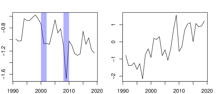
Figure 2: Left panel: estimated first factor with shaded blue areas indicating the dot-com bubble and the financial crisis. Right panel: estimated second factor.

6 Conclusion

In this paper, a new estimator for the regression parameters in a panel data model with interactive fixed effects has been proposed. The main novelty of this approach is that factor loadings are approximated through nonparametric additive functions and it is then possible to partial out the interactive effects. Therefore, the new estimator adopts the well-known partial least squares form, and there is no need to use iterative estimation techniques to compute it. It turns out that the limiting distribution of the estimator has a discontinuity when the variance of the idiosyncratic parameter is near the boundaries. The discontinuity makes the usual ”plug-in” method used to estimate the asymptotic variance only valid pointwise and may produce either over- or under- coveraging probabilities. We show that uniformity can be achieved by cross-sectional bootstrap. Later, the common factors are estimated using principal component analysis (PCA), and the corresponding convergence rates are obtained. A Monte Carlo study indicates good performance in terms of mean squared error. We apply our methodology to analyze the determinants of growth rates in OECD countries.

APPENDIX A: Proofs of Lemmas

Through the Appendix, $C$ denotes a generic positive constant that may be different in different uses and $\mathbf{A}$ is a matrix. Also, when we write $\mathbf{A}\leq C$ for a constant scalar $C$, it means that each element of $\mathbf{A}$ is less or equal to $C$. For scalars or column vectors $A_{it}$ and $B_{it}$, we define $S_{A,B}=(NT)^{-1}\sum_{i,t}\mathbf{A}_{it}\mathbf{B}_{it}^{\top}$ and $S_{A}=S_{A,A}$. We also define the scalar function $\overline{S}_{A}=(NT)^{-1}\sum_{i,t}\mathbf{A}_{it}^{\top}\mathbf{A}_{it}$, which is the sum of the diagonal elements of $S_{A}$. Using $ab\leq(a^{2}+b^{2})/2$ we may write $S_{A,B}\leq\overline{S}_{A}+\overline{S}_{B}$, so the scalar bound $\overline{S}_{A}+\overline{S}_{B}$ bounds each of the elements in $S_{A,B}$. Therefore, if $\overline{S}_{A}+\overline{S}_{B}=\mathcal{O}_{p}(a_{n})$, then each element of $S_{A,B}$ is at most $\mathcal{O}_{p}(a_{n})$, which implies that $S_{A,B}=\mathcal{O}_{p}(a_{n})$, where $a_{n}$ is a positive sequence depending on $n$. Similarly, using the Cauchy-Schwarz inequality we have $S_{A,B}\leq(\overline{S}_{A}\overline{S}_{B})^{1/2}$. Also, for any matrix $\mathbf{A}$ with $N$ rows, we define $\widetilde{A}=\mathbf{P}_{\Phi}(\mathbf{\ddot{X}})\mathbf{A}$.

LEMMA A.1

Under Assumptions 3.3(i) and 3.4(ii), we have, $\|\mathbf{\widetilde{b}}_{h}-\mathbf{b}_{h}\|_{F}=\mathcal{O}_{p}(J^{-\kappa/2})$, where $\mathbf{\widetilde{b}}_{h}=\left[\Phi(\mathbf{\ddot{X}})^{\top}\Phi(\mathbf{\ddot{X}})\right]^{-1}\Phi(\mathbf{\ddot{X}})^{\top}\mathbf{h}$ for $\mathbf{h}=\mathbf{G}(\mathbf{\ddot{X}})$ or $\mathbf{h}=\mathbf{m}(\mathbf{\ddot{X}})$, and $\mathbf{b}_{h}$ is the corresponding $JQ\times K$ or $JQ\times Q$ matrix of sieve coefficients, as $N$ tends to infinity.

Proof. By Assumptions 3.3(i) and 3.4(ii)

$$\|\mathbf{\widetilde{b}}_{h}-\mathbf{b}_{h}\|_{F} = \left\|\left[\Phi(\mathbf{\ddot{X}})^{\top}\Phi(\mathbf{\ddot{X}})\right]^{-1}\Phi(\mathbf{\ddot{X}})^{\top}[\mathbf{h}-\Phi(\mathbf{\ddot{X}})\mathbf{b}_{h}]\right\|_{F}$$

$$\leq \left\|\left[\Phi(\mathbf{\ddot{X}})^{\top}\Phi(\mathbf{\ddot{X}})\right]^{-1}\right\|_{2}\|\Phi(\mathbf{\ddot{X}})\|_{2}\|[\mathbf{h}-\Phi(\mathbf{\ddot{X}})\mathbf{b}_{h}]\|_{F}$$

$$= \mathcal{O}_{p}(J^{-\kappa/2}).$$

${\Box}$

LEMMA A.2

Under Assumptions 3.3(i) and 3.4(ii), $\bar{S}_{h-\widetilde{h}}=N^{-1}\|\mathbf{h}-\mathbf{\widetilde{h}}\|^{2}_{F}=\mathcal{O}_{p}(J^{-\kappa})$, as $N$ tends to infinity, for $\mathbf{h}=\mathbf{G}(\mathbf{\ddot{X}})$ or $\mathbf{h}=\mathbf{m}(\mathbf{\ddot{X}})$, where $\mathbf{\widetilde{h}}=\Phi(\mathbf{\ddot{X}})\mathbf{\widetilde{b}}_{h}$.

Proof. Let

$$\|\mathbf{h}-\mathbf{\widetilde{h}}\|_{F} = \left\|\left[\mathbf{h}-\Phi(\mathbf{\ddot{X}})\mathbf{b}_{h}\right]+\Phi(\mathbf{\ddot{X}})(\mathbf{b}_{h}-\mathbf{\widetilde{b}}_{h})\right\|_{F}$$

$$\leq \|\mathbf{h}-\Phi(\mathbf{\ddot{X}})\mathbf{b}_{h}\|_{F}+\|\Phi(\mathbf{\ddot{X}})(\mathbf{b}_{h}-\mathbf{\widetilde{b}}_{h})\|_{F}.$$

By Lemma A.1 and Assumption 3.3(i), $\|\Phi(\mathbf{\ddot{X}})(\mathbf{b}_{h}-\mathbf{\widetilde{b}}_{h})\|_{F}=\mathcal{O}_{p}(\sqrt{N}J^{-\kappa/2})$ and by Assumption 3.4(ii), $\|\mathbf{h}-\Phi(\mathbf{\ddot{X}})\mathbf{b}_{h}\|_{F}=\mathcal{O}_{p}(\sqrt{N}J^{-\kappa/2})$, as $N$ tends to infinity.  ${\Box}$

LEMMA A.3

Under Assumptions 3.3(i), 3.3(ii), 3.6(i) and 3.6(iii), $\overline{S}_{\widetilde{U}}=O_{p}\left(J/N\right)$, as both $N$ and $T$ tend to infinity, where $\overline{S}_{\widetilde{U}}=(NT)^{-1}\sum_{t=1}^{T}\|\mathbf{\widetilde{u}}_{t}\|^{2}$, and $\mathbf{\widetilde{u}}_{t}=P_{\Phi}(\mathbf{\ddot{X}})\mathbf{u}_{t}$.

Proof. Let

$$\overline{S}_{\widetilde{U}} = (NT)^{-1}\sum_{t=1}^{T}\frac{\mathbf{u}_{t}^{\top}\Phi(\mathbf{\ddot{X}})}{\sqrt{N}}\left[\frac{\Phi(\mathbf{\ddot{X}})^{\top}\Phi(\mathbf{\ddot{X}})}{N}\right]^{-1}\frac{\Phi(\mathbf{\ddot{X}})^{\top}\mathbf{u}_{t}}{\sqrt{N}}$$

$$= (NT)^{-1}\sum_{t=1}^{T}\Big{\|}\left[\frac{\Phi(\mathbf{\ddot{X}})^{\top}\Phi(\mathbf{\ddot{X}})}{N}\right]^{-1/2}\frac{\Phi(\mathbf{\ddot{X}})^{\top}\mathbf{u}_{t}}{\sqrt{N}}\Big{\|}^{2}$$

$$\leq (NT)^{-1}\sum_{t}\Big{\|}\left[\frac{\Phi(\mathbf{\ddot{X}})^{\top}\Phi(\mathbf{\ddot{X}})}{N}\right]^{-1/2}\Big{\|}^{2}_{2}\Big{\|}\frac{\Phi(\mathbf{\ddot{X}})^{\top}\mathbf{u}_{t}}{\sqrt{N}}\Big{\|}^{2}.$$

By Assumption 3.3(i), $\Big{\|}\left[\Phi(\mathbf{\ddot{X}})^{\top}\Phi(\mathbf{\ddot{X}})/N\right]^{-1/2}\Big{\|}^{2}_{2}={\mathcal{O}}_{p}\left(1\right)$, as $N$ tends to infinity and

$$\mathop{\mbox{\sf E}}\Big{\|}\frac{\Phi(\mathbf{\ddot{X}})^{\top}\mathbf{u}_{t}}{\sqrt{N}}\Big{\|}^{2} = N^{-1}\sum^{J}_{j}\sum^{Q}_{q}\mathop{\mbox{\sf E}}\left[\sum^{N}_{i=1}\phi_{j}(\ddot{X}_{iq})u_{it}\right]^{2}$$

$$= N^{-1}\sum_{j}\sum_{q}\sum^{N}_{i=1}\sum^{N}_{i^{\prime}=1}\mathop{\mbox{\sf E}}\left[\phi_{j}(\ddot{X}_{iq})\phi_{j}(\ddot{X}_{i^{\prime}q})\right]\mathop{\mbox{\sf E}}\left(u_{it}u_{i^{\prime}t}\right)$$

$$\leq JQ\max_{j,q,i}\mathop{\mbox{\sf E}}[\phi_{j}(\ddot{X}_{iq})^{2}]\max_{i^{\prime}}\sum^{N}_{i=1}\Big{|}\mathop{\mbox{\sf E}}(u_{it}u_{i^{\prime}t})\Big{|}={\mathcal{O}}\left(J\right).$$

Because of Assumptions 3.3(ii), 3.6(i) and 3.6(iii). Then, to Markov’s inequality

$$\Big{\|}\frac{\Phi(\mathbf{\ddot{X}})^{\top}\mathbf{u}_{t}}{\sqrt{N}}\Big{\|}^{2}={\mathcal{O}}_{p}\left(J\right),$$

and the proof is done.  ${\Box}$

LEMMA A.4

Under assumptions 3.1(iii), 3.3(i) and 3.3(ii), $\bar{S}_{\widetilde{\eta}}=N^{-1}\|\boldsymbol{\widetilde{\eta}}\|^{2}_{F}=\mathcal{O}_{p}\left(J/N\right)$, as $N$ tends to infinity, where $\boldsymbol{\eta}=(\boldsymbol{\eta}_{1},\ldots,\boldsymbol{\eta}_{N})^{\top}$ is a $N\times Q$ matrix, $\boldsymbol{\eta}_{i}=\boldsymbol{\theta}(\mathbf{\ddot{X}}_{i})-\mathbf{m}(\mathbf{\ddot{X}}_{i})$ and $\boldsymbol{\widetilde{\eta}}=\mathbf{P}_{\Phi}(\mathbf{\ddot{X}})\boldsymbol{\eta}$.

Proof. The proof follows the same lines as in the proof of Lemma A.3. Therefore we omit the common parts. Noting that

$$\bar{S}_{\widetilde{\eta}}=N^{-1}\left\|\left[\frac{\Phi(\mathbf{\ddot{X}})^{\top}\Phi(\mathbf{\ddot{X}})}{N}\right]^{-1/2}\frac{\Phi(\mathbf{\ddot{X}})^{\top}\boldsymbol{\eta}}{\sqrt{N}}\right\|^{2}_{F},$$

by Assumption 3.3(i), $\Big{\|}\left[\Phi(\mathbf{\ddot{X}})^{\top}\Phi(\mathbf{\ddot{X}})/N\right]^{-1/2}\Big{\|}^{2}_{2}={\mathcal{O}}_{p}\left(1\right)$, as $N$ tends to infinity. Under assumptions 3.1(iii) and 3.3(ii) we obtain that

$$\mathop{\mbox{\sf E}}\left\|\frac{\Phi(\mathbf{\ddot{X}})^{\top}\boldsymbol{\eta}}{\sqrt{N}}\right\|_{F}^{2} = \frac{1}{N}{\rm tr}\mathop{\mbox{\sf E}}[\Phi(\mathbf{\ddot{X}})\Phi(\mathbf{\ddot{X}})^{\top}\boldsymbol{\eta}\boldsymbol{\eta}^{\top}]\leq\frac{C}{N}{\rm tr}\mathop{\mbox{\sf E}}[\Phi(\mathbf{\ddot{X}})\Phi(\mathbf{\ddot{X}})^{\top}]=\mathcal{O}(J),$$

and applying Markov’s inequality we have $\Big{\|}\Phi(\mathbf{\ddot{X}})^{\top}\boldsymbol{\eta}/\sqrt{N}\Big{\|}^{2}_{F}=\mathcal{O}_{p}(J)$ and the proof of the lemma is done.  ${\Box}$

LEMMA A.5

Under assumptions 3.1(ii), 3.3(i) and 3.3(ii), $\bar{S}_{\widetilde{\varepsilon}}=(NT)^{-1}\sum^{T}_{t=1}\|\boldsymbol{\widetilde{\varepsilon}}_{t}\|^{2}_{F}=\mathcal{O}_{p}\left(J/N\right)$, as both $N$ and $T$ tend to infinity, where $\boldsymbol{\varepsilon}=(\boldsymbol{\varepsilon}_{1t},\ldots,\boldsymbol{\varepsilon}_{Nt})^{\top}$ is a $N\times Q$ matrix, $\boldsymbol{\varepsilon}_{it}=\mathbf{X}_{it}-\theta(\mathbf{\ddot{X}}_{i})$ and $\boldsymbol{\widetilde{\varepsilon}}_{t}=\mathbf{P}_{\Phi}(\mathbf{\ddot{X}})\boldsymbol{\varepsilon}_{t}$.

Proof. Let

$$\bar{S}_{\widetilde{\varepsilon}} = (NT)^{-1}\sum_{t=1}^{T}\Big{\|}\left[\Phi(\mathbf{\ddot{X}})^{\top}\Phi(\mathbf{\ddot{X}})/N\right]^{-1/2}\Phi(\mathbf{\ddot{X}})^{\top}\boldsymbol{\varepsilon}_{t}/\sqrt{N}\Big{\|}^{2}_{F}.$$

Following a similar reasoning as in Lemmas A.3 and A.4 it is straightforward to show that under assumptions 3.1(ii) and 3.3(ii), $\|\Phi(\mathbf{\ddot{X}})^{\top}\boldsymbol{\varepsilon}_{t}/\sqrt{N}\|_{F}^{2}={\mathcal{O}}_{p}\left(J\right)$, as $N\rightarrow\infty$. Then the proof is closed.  ${\Box}$

LEMMA A.6

Under Assumptions 3.2, 3.3(ii), 3.5)(i) and 3.5(ii),

$$\bar{S}_{\widetilde{\Gamma}f}=(NT)^{-1}\sum_{t=1}^{T}\|\widetilde{\boldsymbol{\Gamma}}\mathbf{f}_{t}\|^{2}={\mathcal{O}}_{p}\left(J\nu_{N}/N\right),$$

as both $N$ and $T$ tend to infinity and $\widetilde{\boldsymbol{\Gamma}}=\mathbf{P}_{\Phi}(\mathbf{\ddot{X}})\boldsymbol{\Gamma}$.

Proof. Proceeding as in the proof of previous lemmas, by idempotence of $\mathbf{P}_{\Phi}(\mathbf{\ddot{X}})$ we have

$$\overline{S}_{\widetilde{\Gamma}f} = (NT)^{-1}\sum_{t=1}^{T}\Big{\|}\left[\Phi(\mathbf{\ddot{X}})^{\top}\Phi(\mathbf{\ddot{X}})/N\right]^{-1/2}\Phi(\mathbf{\ddot{X}})^{\top}\boldsymbol{\Gamma}\mathbf{f}_{t}/\sqrt{N}\Big{\|}^{2}$$

$$\leq (NT)^{-1}\sum_{t=1}^{T}\Big{\|}\left[\Phi(\mathbf{\ddot{X}})^{\top}\Phi(\mathbf{\ddot{X}})/N\right]^{-1/2}\Big{\|}^{2}_{2}\Big{\|}\Phi(\mathbf{\ddot{X}})^{\top}\boldsymbol{\Gamma}\mathbf{f}_{t}/\sqrt{N}\Big{\|}^{2}$$

$$= N^{-1}\Big{\|}\left[\Phi(\mathbf{\ddot{X}})^{\top}\Phi(\mathbf{\ddot{X}})/N\right]^{-1/2}\Big{\|}^{2}_{2}\Big{\|}\Phi(\mathbf{\ddot{X}})^{\top}\boldsymbol{\Gamma}/\sqrt{N}\Big{\|}^{2}_{F}.$$

The last equality is obtained by using Assumption 3.2 and applying the properties of the trace operator. Now, by Assumption 3.3(i), $\Big{\|}\left[\Phi(\mathbf{\ddot{X}})^{\top}\Phi(\mathbf{\ddot{X}})/N\right]^{-1/2}\Big{\|}^{2}_{2}={\mathcal{O}}_{p}\left(1\right)$, as $N$ tends to infinity, and since $\ddot{X}_{iq}$ and $\gamma_{ik}$ are independent and $\mathop{\mbox{\sf E}}(\gamma_{ik})=0$, (see Assumption (3.5)(i) and applying assumptions 3.3(ii) and 3.5(ii)

$$\mathop{\mbox{\sf E}}\Big{\|}\Phi(\mathbf{\ddot{X}})^{\top}\boldsymbol{\Gamma}\Big{\|}^{2}_{F} = \sum_{j=1}^{J}\sum_{k=1}^{K}\sum_{q=1}^{Q}\mathop{\mbox{\sf E}}\left[\sum^{N}_{i=1}\phi_{j}(\ddot{X}_{iq})\gamma_{ik}\right]^{2}=\sum_{j=1}^{J}\sum_{k=1}^{K}\sum_{q=1}^{Q}{\sf Var}\left[\sum^{N}_{i=1}\phi_{j}(\ddot{X}_{iq})\gamma_{ik}\right]$$

$$= \sum_{j=1}^{J}\sum_{k=1}^{K}\sum_{q=1}^{Q}\sum^{N}_{i=1}{\sf Var}\left[\phi_{j}(\ddot{X}_{iq})\gamma_{ik}\right]+\sum_{j=1}^{J}\sum_{k=1}^{K}\sum_{q=1}^{Q}\sum^{N}_{i\neq i^{\prime}}{\sf Cov}\left[\phi_{j}(\ddot{X}_{iq})\gamma_{ik},\phi_{j}(\ddot{X}_{i^{\prime}q})\gamma_{i^{\prime}k}\right]$$

$$= \sum_{j=1}^{J}\sum_{k=1}^{K}\sum_{q=1}^{Q}\sum^{N}_{i=1}\mathop{\mbox{\sf E}}[\phi_{j}(\ddot{X}_{iq})^{2}]\mathop{\mbox{\sf E}}(\gamma^{2}_{ik})+\sum_{j=1}^{J}\sum_{k=1}^{K}\sum_{q=1}^{Q}\sum^{N}_{i\neq i^{\prime}}\mathop{\mbox{\sf E}}\left[\phi_{j}(\ddot{X}_{iq})\phi_{j}(\ddot{X}_{i^{\prime}q})\right]\mathop{\mbox{\sf E}}\left(\gamma_{ik}\gamma_{i^{\prime}k}\right)$$

$$= {\mathcal{O}}\left(NJ\nu_{N}\right)+{\mathcal{O}}\left(NJ\right)\max_{k}\max_{i^{\prime}}\sum^{N}_{i=1}\left|\mathop{\mbox{\sf E}}(\gamma_{ik}\gamma_{i^{\prime}k})\right|,$$

and $\max_{k}\max_{i^{\prime}}\sum^{N}_{i=1}\left|\mathop{\mbox{\sf E}}(\gamma_{ik}\gamma_{i^{\prime}k})\right|={\mathcal{O}}\left(\nu_{N}\right)$ because of Assumption 3.5(ii). Now apply Markov’s inequality and the proof is closed.  ${\Box}$

LEMMA A.7

Let us define $\mathbf{\widetilde{\boldsymbol{\beta}}}$ as

$$\widetilde{\boldsymbol{\beta}}=\left\{\sum_{t=1}^{T}\mathbf{X}_{t}^{\top}[\mathbf{I}_{N}-\mathbf{P}_{\Phi}(\mathbf{\ddot{X}})]\mathbf{X}_{t}\right\}^{-1}\sum_{t=1}^{T}\mathbf{X}_{t}^{\top}[\mathbf{I}_{N}-\mathbf{P}_{\Phi}(\mathbf{\ddot{X}})]\mathbf{y}_{t},$$ (I.1)

where

$$\mathbf{\mathbf{missing}}{P}_{\Phi}(\mathbf{\ddot{X}}) = \Phi(\mathbf{\ddot{X}})\left[\Phi(\mathbf{\ddot{X}})^{\top}\Phi(\mathbf{\ddot{X}})\right]^{-1}\Phi(\mathbf{\ddot{X}})$$

$$\Phi(\mathbf{\ddot{X}}) = (\phi(\mathbf{\ddot{X}}_{1}),\ldots,\phi(\mathbf{\ddot{X}}_{N}))^{\top},$$

$$\phi(\mathbf{\ddot{X}}_{i})^{\top} = (\phi_{1}(\ddot{X}_{i1}),\ldots,\phi_{J}(\ddot{X}_{i1}),\ldots,\phi_{1}(\ddot{X}_{iQ}),\ldots,\phi_{J}(\ddot{X}_{iQ})).$$

Under assumptions 3.1(iv) - 3.7 and if it is further assumed that $J/\sqrt{N}\rightarrow 0$ and $\nu_{N}\sim T^{-\alpha}$, as both $N$ and $T$ tends to infinity, then for $\alpha\in[0,1)$

$$\sqrt{NT^{\alpha}}(\widetilde{\boldsymbol{\beta}}-\boldsymbol{\beta})\stackrel{{\scriptstyle\mathcal{L}}}{{\rightarrow}}N\left(0,\widetilde{V}^{-1}_{\xi}\widetilde{V}_{\Gamma}\widetilde{V}^{-1}_{\xi}\right).$$ (I.2)

Under the same set of assumptions, if $\alpha=1$

$$\sqrt{NT}(\widetilde{\boldsymbol{\beta}}-\boldsymbol{\beta})\stackrel{{\scriptstyle\mathcal{L}}}{{\rightarrow}}N\left(0,\widetilde{V}^{-1}_{\xi}\left(\widetilde{V}_{\Gamma}+\widetilde{V}_{u}\right)\widetilde{V}^{-1}_{\xi}\right),$$ (I.3)

and finally if $\alpha>1$

$$\sqrt{NT}(\widetilde{\boldsymbol{\beta}}-\boldsymbol{\beta})\stackrel{{\scriptstyle\mathcal{L}}}{{\rightarrow}}N\left(0,\widetilde{V}^{-1}_{\xi}\widetilde{V}_{u}\widetilde{V}^{-1}_{\xi}\right),$$ (I.4)

where

$$\widetilde{V}_{\xi} \stackrel{{\scriptstyle\operatorname{def}}}{{=}} \operatorname{plim}_{N,T\rightarrow\infty}\frac{1}{NT}\sum^{T}_{t=1}\boldsymbol{\xi}^{\top}_{t}\boldsymbol{\xi}_{t}$$ (I.5)

$$\widetilde{V}_{\Gamma} \stackrel{{\scriptstyle\operatorname{def}}}{{=}} \sum_{k\leq K;k^{\prime}\leq K}\mathop{\mbox{\sf E}}\left[\gamma_{ik}\gamma_{ik^{\prime}}\mathop{\mbox{\sf E}}\left(\left.\xi_{it}f_{tk}\right|\boldsymbol{\Gamma}\right)\mathop{\mbox{\sf E}}\left(\left.\boldsymbol{\xi}_{it}f_{tk^{\prime}}\right|\boldsymbol{\Gamma}\right)^{\top}\right],$$ (I.6)

$$\widetilde{V}_{u} \stackrel{{\scriptstyle\operatorname{def}}}{{=}} \operatorname{lim}_{N,T\to\infty}\frac{1}{NT}\sum_{t=1}^{T}\sum_{\ell=-\infty}^{+\infty}\mathop{\mbox{\sf E}}(\boldsymbol{\xi}_{t}^{\top}\mathbf{u}_{t}\mathbf{u}_{t-\ell}^{\top}\boldsymbol{\xi}_{t-\ell}).$$ (I.7)

Proof.

For the sake of simplicity, we will use the following shorthand notations: $\boldsymbol{\theta}_{i}=\theta(\mathbf{\ddot{X}}_{i})$, $\mathbf{m}_{i}=\mathbf{m}\left(\mathbf{\ddot{X}}_{i}\right)$. Furthermore, recall that $\boldsymbol{\varepsilon}_{it}=\mathbf{X}_{it}-\boldsymbol{\theta}_{i}$, $\boldsymbol{\eta}_{i}=\boldsymbol{\theta}_{i}-\mathbf{m}_{i}$ and $\boldsymbol{\xi}_{it}=\mathbf{X}_{it}-\mathbf{m}_{i}$. Then, we can write $\mathbf{X}_{it}=\boldsymbol{\varepsilon}_{it}+\boldsymbol{\eta}_{i}+\mathbf{m}_{i}$ and $\tilde{\mathbf{X}}_{it}=\boldsymbol{\tilde{\varepsilon}}_{it}+\boldsymbol{\tilde{\eta}}_{i}+\boldsymbol{\tilde{m}}_{i}$. By subtracting these quantities it yields

$$\mathbf{X}_{it}-\tilde{\mathbf{X}}_{it}=(\boldsymbol{\varepsilon}_{it}-\boldsymbol{\tilde{\varepsilon}}_{it})+(\boldsymbol{\eta}_{i}-\boldsymbol{\tilde{\eta}}_{i})+(\boldsymbol{\tilde{m}}_{i}-\boldsymbol{m}_{i}).\quad$$ (I.8)

Plugging (7) into (I.1) and using the idempotent property of $\mathbf{P}_{\Phi}(\mathbf{\ddot{X}})$, then

$$\widetilde{\boldsymbol{\beta}}-\boldsymbol{\beta} = \left[\frac{1}{NT}\sum^{T}_{t=1}(\mathbf{X}_{t}-\widetilde{\mathbf{X}}_{t})^{\top}(\mathbf{X}_{t}-\widetilde{\mathbf{X}}_{t})\right]^{-1}$$

$$\times \frac{1}{NT}\sum^{T}_{t=1}(\mathbf{X}_{t}-\widetilde{\mathbf{X}}_{t})^{\top}\left[(\mathbf{G}(\mathbf{\bar{X}})-\widetilde{G}(\mathbf{\bar{X}}))\mathbf{f}_{t}+(\mathbf{v}_{t}-\widetilde{\mathbf{v}}_{t})\right],$$

and defining,

$$S_{X-\widetilde{X}} \stackrel{{\scriptstyle\text{def}}}{{=}} \frac{1}{NT}\sum^{T}_{t=1}(\mathbf{X}_{t}-\widetilde{\mathbf{X}}_{t})^{\top}(\mathbf{X}_{t}-\widetilde{\mathbf{X}}_{t}),$$ (I.9)

$$S_{X-\widetilde{X},(G-\widetilde{G})f} \stackrel{{\scriptstyle\text{def}}}{{=}} \frac{1}{NT}\sum^{T}_{t=1}(\mathbf{X}_{t}-\widetilde{\mathbf{X}}_{t})^{\top}[\mathbf{G}(\mathbf{\bar{X}})-\widetilde{\mathbf{G}}(\mathbf{\bar{X}})]\mathbf{f}_{t}$$ (I.10)

$$S_{X-\widetilde{X},V-\widetilde{V}} \stackrel{{\scriptstyle\text{def}}}{{=}} \frac{1}{NT}\sum^{T}_{t=1}(\mathbf{X}_{t}-\widetilde{\mathbf{X}}_{t})^{\top}(\mathbf{v}_{t}-\widetilde{\mathbf{v}}_{t}),$$ (I.11)

we have that

$$\sqrt{NT^{\alpha}}(\widetilde{\boldsymbol{\beta}}-\boldsymbol{\beta})=S^{-1}_{X-\widetilde{X}}\times\sqrt{NT^{\alpha}}\left(S_{X-\widetilde{X},(G-\widetilde{G})f}+S_{X-\widetilde{X},V-\widetilde{V}}\right),$$

where $\widetilde{G}(\mathbf{\bar{X}})=\mathbf{P}_{\Phi}(\mathbf{\ddot{X}})\mathbf{G}(\mathbf{\bar{X}})$, $\mathbf{\widetilde{X}}_{t}=\mathbf{P}_{\Phi}(\mathbf{\ddot{X}})\mathbf{X}_{t}$, $\widetilde{\mathbf{v}}_{t}=\mathbf{P}_{\Phi}(\mathbf{\ddot{X}})\mathbf{v}_{t}$ and $\mathbf{v}_{t}=\boldsymbol{\Gamma}\mathbf{f}_{t}+\mathbf{u}_{t}$.

Defining $\boldsymbol{\xi}_{t}^{\top}$ as a $Q\times N$ matrix such as $\boldsymbol{\xi}_{t}^{\top}=(\boldsymbol{\xi}_{1t},\ldots,\boldsymbol{\xi}_{Nt})$, we will obtain the asymptotic distribution of $\widetilde{\boldsymbol{\beta}}$, by showing the following results:

• $S_{X-\widetilde{X}}=\widetilde{V}_{\xi}+{\scriptstyle\mathcal{O}}_{p}(1)$,

• $S_{X-\widetilde{X},(G-\widetilde{G})f}={\scriptstyle\mathcal{O}}_{p}\left((NT)^{-1/2}\right)$,

• $S_{X-\widetilde{X},\widetilde{V}}={\scriptstyle{\mathcal{O}}}_{p}((NT)^{-1/2})+{\scriptstyle{\mathcal{O}}}_{p}(N^{-1/2}\nu_{N}^{1/2})$,

• $\sqrt{NT^{\alpha}}S_{(X-\tilde{X}),V}\stackrel{{\scriptstyle\mathcal{L}}}{{\rightarrow}}N(0,\widetilde{V}_{\alpha})$,

where $\widetilde{V}_{\alpha}$, with a slight abuse of notation, stands for the asymptotic variance-covariance matrix of $\widetilde{\boldsymbol{\beta}}$ such that,

$$\widetilde{V}_{\alpha}=\left\{\begin{array}[]{lc}\widetilde{V}^{-1}_{\xi}\widetilde{V}_{\Gamma}\widetilde{V}^{-1}_{\xi},\qquad{\rm for}\ \alpha\in[0,1),\\ \widetilde{V}^{-1}_{\xi}\left(\widetilde{V}_{\Gamma}+\widetilde{V}_{u}\right)\widetilde{V}^{-1}_{\xi},\qquad{\rm for}\ \alpha=1,\\ \widetilde{V}^{-1}_{\xi}\widetilde{V}_{u}\widetilde{V}^{-1}_{\xi},\qquad{\rm for}\ \alpha>1.\end{array}\right.$$

Proof of (i): Using (I.8), $S_{X-\widetilde{X}}$ can be decomposed as

$$S_{X-\widetilde{X}}=S_{\eta+\varepsilon+(m-\widetilde{m})-\widetilde{\eta}-\widetilde{\varepsilon}}=S_{\eta+\varepsilon}+S_{(m-\widetilde{m})-\widetilde{\eta}-\widetilde{\varepsilon}}+2S_{\eta+\varepsilon,(m-\widetilde{m})-\widetilde{\eta}-\widetilde{\varepsilon}},$$ (I.13)

where each element has to be considered separately. Focusing on the first element of the right-hand side of (I.13), we get

$$S_{\eta+\varepsilon}=(NT)^{-1}\sum^{T}_{t=1}(\boldsymbol{\eta}+\boldsymbol{\varepsilon}_{t})^{\top}(\boldsymbol{\eta}+\boldsymbol{\varepsilon}_{t})=(NT)^{-1}\sum^{T}_{t=1}\boldsymbol{\xi}_{t}^{\top}\boldsymbol{\xi}_{t},$$ (I.14)

where $\boldsymbol{\eta}=(\boldsymbol{\eta}_{1},\ldots,\boldsymbol{\eta}_{N})^{\top}$ and $\boldsymbol{\varepsilon}_{t}=(\boldsymbol{\varepsilon}_{1t},\ldots,\boldsymbol{\varepsilon}_{Nt})^{\top}$ are $N\times Q$ matrices.

$S_{(m-\widetilde{m})-\widetilde{\eta}-\widetilde{\varepsilon}}=\mathcal{O}_{p}(J^{-2\kappa})+\mathcal{O}_{p}\left(J/N\right)={\scriptstyle\mathcal{O}}_{p}(1)$, because $S_{(m-\widetilde{m})-\widetilde{\eta}-\widetilde{\varepsilon}}\leq 2\overline{S}_{m-\widetilde{m}}+4\overline{S}_{\widetilde{\eta}}+4\overline{S}_{\widetilde{\varepsilon}}$. Then, applying respectively lemmas A.2, A.4 and A.5 we have that $\overline{S}_{m-\widetilde{m}}=\mathcal{O}_{p}(J^{-\kappa})$, $\overline{S}_{\widetilde{\eta}}=\overline{S}_{\widetilde{\varepsilon}}=\mathcal{O}_{p}\left(J/N\right)$. Finally, the third term in (I.13) is ${\scriptstyle\mathcal{O}}_{p}(1)$ because given that $(\eta+\varepsilon)$ is orthogonal to the functional space $\mathcal{G}$ and $m-\widetilde{m}$ belongs to $\mathcal{G}$, by the Cauchy-Schwarz inequality we obtain that $S_{\eta+\varepsilon,(m-\widetilde{m})-\widetilde{\eta}-\widetilde{\varepsilon}}\leq\overline{S}^{1/2}_{\eta+\varepsilon}\overline{S}^{1/2}_{(m-\widetilde{m})-\widetilde{\eta}-\widetilde{\varepsilon}}=\mathcal{O}_{p}(1)\times{\scriptstyle\mathcal{O}}_{p}(1)={\scriptstyle\mathcal{O}}_{p}(1)$. Now apply Assumption 3.1(iv) to (I.14) and this ends the proof of (i).

Proof of (ii): By the idempotent property of $\mathbf{M}_{\Phi}(\mathbf{\ddot{X}})=\mathbf{I}_{N}-\mathbf{P}_{\Phi}(\mathbf{\ddot{X}})$

$$S_{X-\widetilde{X},(G-\widetilde{G})f} = \frac{1}{NT}\sum_{t=1}^{T}\mathbf{X}_{t}^{\top}\mathbf{M}_{\Phi}(\mathbf{\ddot{X}})\mathbf{G}(\mathbf{\bar{X}})\mathbf{f}_{t}$$

$$= \frac{1}{NT}\sum_{t=1}^{T}\left(\mathbf{X}_{t}-\widetilde{\mathbf{X}}_{t}\right)^{\top}\left[\mathbf{G}(\mathbf{\ddot{X}})-\widetilde{\mathbf{G}}(\mathbf{\ddot{X}})\right]\mathbf{f}_{t}$$

$$+ \frac{1}{NT}\sum_{t=1}^{T}\left(\mathbf{X}_{t}-\widetilde{\mathbf{X}}_{t}\right)^{\top}\left\{\left[\mathbf{G}(\mathbf{\bar{X}})-\mathbf{G}(\mathbf{\ddot{X}})\right]-\left[\widetilde{\mathbf{G}}(\mathbf{\bar{X}})-\widetilde{\mathbf{G}}(\mathbf{\ddot{X}})\right]\right\}\mathbf{f}_{t}$$

$$\stackrel{{\scriptstyle\text{def}}}{{=}} \mathcal{I}_{1}+\mathcal{I}_{2}.$$

Applying the Cauchy-Schwarz inequality then

$$\mathcal{I}_{1}\leq\bar{S}^{1/2}_{(X-\widetilde{X})}\bar{S}^{1/2}_{(G(\ddot{X})-\widetilde{G}(\ddot{X}))f}.$$

By (i), $\bar{S}_{(X-\widetilde{X})}=\mathcal{O}_{p}(1)$ and $\bar{S}_{(G(\ddot{X})-\widetilde{G}(\ddot{X}))f}=\mathcal{O}_{p}(J^{-\kappa})$. This last result follows from recalling that by the trace properties and Lemma A.2

$$\bar{S}_{(G(\ddot{X})-\widetilde{G}(\ddot{X}))f}=N^{-1}{\rm tr}\{[\mathbf{G}(\mathbf{\ddot{X}})-\widetilde{\mathbf{G}}(\mathbf{\ddot{X}})][\mathbf{G}(\mathbf{\ddot{X}})-\widetilde{\mathbf{G}}(\mathbf{\ddot{X}})]^{\top}\}.$$

Following the same lines as before, using the trace properties and assumptions 3.1(i), 3.2, 3.4(ii), 3.5(ii) and a Taylor expansion of $\mathbf{G}(\mathbf{\bar{X}})$ around $\mathbf{G}(\mathbf{\ddot{X}})$ it is possible to prove that $\mathcal{I}_{2}=\mathcal{O}_{p}(J^{-\kappa}/T)={\scriptstyle\mathcal{O}}_{p}(J^{-\kappa})$. Finally, since $\sqrt{NT}J^{-\kappa/2}\to 0$ by Assumption 3.4(iii), we have $S_{X-\widetilde{X},(G-\widetilde{G})f}={\scriptstyle\mathcal{O}}_{p}\left((NT)^{-1/2}\right)$, as $T$ tends to infinity.

Proof of (iii):

Using (I.8), $S_{X-\widetilde{X},\widetilde{V}}$ can be written as

$$S_{X-\widetilde{X},\widetilde{V}}=S_{\xi,\widetilde{V}}+S_{(m-\widetilde{m}),\widetilde{V}}-S_{\widetilde{\varepsilon},\widetilde{V}}-S_{\widetilde{\eta},\widetilde{V}}.$$ (I.15)

We will show that, as $N,T\rightarrow\infty$ and $J={\scriptstyle\mathcal{O}}(\sqrt{N})$,

$$S_{\xi,\widetilde{V}}={\scriptstyle\mathcal{O}}_{p}\left(1/{\sqrt{NT}}\right)+{\scriptstyle\mathcal{O}}_{p}\left(\nu^{1/2}_{N}/\sqrt{N}\right).$$ (I.16)

In order to show it, recalling that $\widetilde{\mathbf{V}}=\widetilde{\boldsymbol{\Gamma}}\mathbf{f}+\widetilde{\mathbf{U}}$, the first term in (I.15) can be decomposed as

$$S_{\xi,\widetilde{V}} =S_{\xi,\widetilde{U}}+S_{\xi,\widetilde{\Gamma}f}.$$ (I.17)

$$S_{\xi,\widetilde{U}} = (NT)^{-1}\sum^{T}_{t=1}\boldsymbol{\xi}_{t}^{\top}\widetilde{\mathbf{u}}_{t}={\scriptstyle\mathcal{O}}_{p}\left(\frac{1}{\sqrt{NT}}\right),$$ (I.18)

as both $N$ and $T$ tend to infinity. The proof follows by noting that

$$S_{\xi,\widetilde{U}}\leq\left\|\boldsymbol{\xi}^{\top}_{t}\Phi(\mathbf{\ddot{X}})\right\|_{F}\left\|\left[\Phi^{\top}(\mathbf{\ddot{X}})\Phi(\mathbf{\ddot{X}})\right]^{-1}\right\|_{2}\frac{1}{NT}\|\Phi(\mathbf{\ddot{X}})^{\top}\mathbf{U}\|_{F}.$$

By assumptions 3.1(ii) and 3.3(ii) we have that

$$\left\|\boldsymbol{\xi}^{\top}_{t}\Phi(\mathbf{\ddot{X}})\right\|_{F}=\mathcal{O}_{p}\left(\sqrt{NJ}\right).$$

Assumption 3.3(i) directly implies that

$$\left\|\left[\Phi^{\top}(\mathbf{\ddot{X}})\Phi(\mathbf{\ddot{X}})\right]^{-1}\right\|_{2}=\mathcal{O}_{p}\left(N^{-1}\right),$$

and finally by assumptions 3.3(ii), 3.6(i) and 3.6(iii) we obtain

$$\|\Phi(\mathbf{\ddot{X}})^{\top}\mathbf{U}\|_{F}=\mathcal{O}_{p}\left(\sqrt{NTJ}\right).$$

The proof of (I.18) is finished by noting that $J/\sqrt{N}\rightarrow 0$ as $N$ tends to infinity.
For the second term in (I.17) we obtain

$$S_{\xi,\widetilde{\boldsymbol{\Gamma}}f} = (NT)^{-1}\sum^{T}_{t=1}\boldsymbol{\xi}_{t}^{\top}\mathbf{P}_{\Phi}(\mathbf{\ddot{X}})\boldsymbol{\Gamma}\mathbf{f}_{t}$$ (I.19)

$$= {\scriptstyle\mathcal{O}}_{p}\left(\sqrt{\nu_{N}/N}\right).$$

To show this, note that

$$S_{\xi,\widetilde{\Gamma}f} = (NT)^{-1}\sum^{T}_{t=1}\boldsymbol{\xi}_{t}^{\top}\Phi(\mathbf{\ddot{X}})\left[\Phi(\mathbf{\ddot{X}})^{\top}\Phi(\mathbf{\ddot{X}})\right]^{-1}\Phi(\mathbf{\ddot{X}})^{\top}\boldsymbol{\Gamma}\mathbf{f}_{t}$$

$$\leq (NT)^{-1}\sum^{T}_{t=1}\|\boldsymbol{\xi}_{t}^{\top}\Phi(\mathbf{\ddot{X}})\|_{F}\left\|\left[\Phi(\mathbf{\ddot{X}})^{\top}\Phi(\mathbf{\ddot{X}})\right]^{-1}\right\|_{2}\|\Phi(\mathbf{\ddot{X}})^{\top}\boldsymbol{\Gamma}\mathbf{f}_{t}\|,$$

but by assumptions 3.1(ii) and 3.3(i), $\|\boldsymbol{\xi}_{t}^{\top}\Phi(\mathbf{\ddot{X}})\|_{F}\lesssim_{p}N^{1/2}(JQ)^{1/2}$, by Assumption 3.3(i), $\left\|\left[N^{-1}\Phi(\mathbf{\ddot{X}})^{\top}\Phi(\mathbf{\ddot{X}})\right]^{-1}\right\|_{2}\lesssim_{p}1$ and finally, by assumptions 3.2 and 3.5, $\|\Phi(\mathbf{\ddot{X}})^{\top}\boldsymbol{\Gamma}\mathbf{f}_{t}\|\lesssim_{p}(N)^{1/2}(JQ)^{1/2}\nu_{N}^{1/2}$. Now assuming that $J={\scriptstyle\mathcal{O}}(\sqrt{N})$, (I.19) is proved. Finally, plugging (I.18)-(I.19) into $S_{\varepsilon+\eta,\widetilde{V}}$ the proof of (I.16) is closed.

Focusing now on the second term of the right-hand side of (I.15), by assumptions 3.2, 3.3(i)-(ii), 3.4(ii) and 3.5(ii) it can be proved

$$S_{(m-\widetilde{m}),\widetilde{V}} = \frac{1}{NT}\sum^{T}_{t=1}(\mathbf{m}-\mathbf{\widetilde{m}})^{\top}(\widetilde{\boldsymbol{\Gamma}}\mathbf{f}_{t}+\widetilde{\mathbf{u}}_{t})$$

$$\leq [\overline{S}_{(m-\widetilde{m})}\overline{S}_{\widetilde{\Gamma}f}]^{1/2}+[\overline{S}_{(m-\widetilde{m})}\overline{S}_{\widetilde{U}}]^{1/2}$$

$$= {\mathcal{O}}_{p}(J^{-\kappa/2}){\mathcal{O}}_{p}\left(\frac{\sqrt{J}\nu_{N}^{1/2}}{\sqrt{N}}\right)+{\mathcal{O}}_{p}(J^{-\kappa/2}){\mathcal{O}}_{p}\left(\frac{\sqrt{J}}{\sqrt{N}}\right),$$

where the last equality follows from Lemmas A.2-A.3 and A.6. Then, using the above result we can conclude

$$S_{(m-\widetilde{m}),\widetilde{V}}={\scriptstyle{\mathcal{O}}}_{p}\left(\frac{\nu_{N}^{1/2}}{\sqrt{NT}}\right)+{\scriptstyle{\mathcal{O}}}_{p}\left(\frac{1}{\sqrt{NT}}\right)$$ (I.20)

since by Assumption 3.4(iii) $\sqrt{NT}J^{-\kappa/2}\rightarrow 0$, as $N$ and $T$ goes to infinity.

In order to end the proof of (iii) we show that

$$S_{\widetilde{\varepsilon},\widetilde{V}}={\scriptstyle{\mathcal{O}}}_{p}\left(\frac{\nu_{N}^{1/2}}{\sqrt{N}}\right)+{\scriptstyle{\mathcal{O}}}_{p}\left(\frac{1}{\sqrt{NT}}\right),$$ (I.21)

$$S_{\widetilde{\eta},\widetilde{V}}={\scriptstyle{\mathcal{O}}}_{p}\left(\frac{\nu_{N}^{1/2}}{\sqrt{N}}\right)+{\scriptstyle{\mathcal{O}}}_{p}\left(\frac{1}{\sqrt{NT}}\right),$$ (I.22)

as both $N$ and $T$ tend to infinity. The proof is straightforward by noting that, by the idempotent property of $\mathbf{P}_{\Phi}(\mathbf{\ddot{X}})$, $S_{\widetilde{\varepsilon},\widetilde{V}}=S_{\varepsilon,\widetilde{\Gamma}f}+S_{\varepsilon,\widetilde{U}}$ and $S_{\widetilde{\eta},\widetilde{V}}=S_{\eta,\widetilde{\Gamma}f}+S_{\eta,\widetilde{U}}$. Using results (I.18) and (I.19) and proceeding as in the proof of (I.19) we can show that $S_{\varepsilon,\widetilde{\Gamma}f}={\mathcal{O}}_{p}\left(J\nu_{N}^{1/2}/N\right)$ and $S_{\eta,\widetilde{\Gamma}f}={\mathcal{O}}_{p}\left(J\nu_{N}^{1/2}/N\right)$. Again, assuming that $J/\sqrt{N}\rightarrow 0$, as $N$ and $T$ goes to infinity, the proofs of (I.21)-(I.22) are done. Finally, replacing (I.16) and (I.20)-(I.22) in (I.15) the proof of (iii) is done.

Proof of (iv):

Using (I.8), we have

$$S_{(X-\tilde{X}),V} = S_{\eta+\varepsilon+(m-\tilde{m})-\tilde{\eta}-\tilde{\varepsilon},V}$$ (I.23)

$$= S_{\eta+\varepsilon,V}+S_{(m-\tilde{m}),V}-S_{\tilde{\eta},V}-S_{\tilde{\varepsilon},V}.$$

Let

$$S_{(m-\tilde{m}),V} = S_{(m-\tilde{m}),\Gamma f}+S_{(m-\tilde{m}),U}.$$

By the Cauchy-Schwarz inequality

$$S_{(m-\tilde{m}),\Gamma f} \leq \bar{S}^{1/2}_{(m-\tilde{m})}\bar{S}^{1/2}_{\Gamma f}.$$

Applying directly Lemma A.2 we have $S_{(m-\tilde{m}),\Gamma f}={\scriptstyle{\mathcal{O}}}_{p}\left(\sqrt{\nu_{N}/NT}\right)$, because under Assumption 3.5(ii), $\bar{S}_{\Gamma f}=\mathcal{O}_{p}(\nu_{N})$. Proceeding in a similar way and applying Lemma A.2 we obtain $S_{(m-\tilde{m}),U}={\scriptstyle{\mathcal{O}}}_{p}\left(1/\sqrt{NT}\right)$ because under assumptions 3.6(i) and 3.6(iii), $\bar{S}_{U}=\mathcal{O}_{p}(1)$. Therefore, $S_{(m-\tilde{m}),V}={\scriptstyle{\mathcal{O}}}_{p}\left(\sqrt{\nu_{N}/NT}\right)+{\scriptstyle{\mathcal{O}}}_{p}\left(1/\sqrt{NT}\right)$. Furthermore, by idempotence of $\mathbf{P}_{\Phi}(\mathbf{\ddot{X}})$, $S_{\tilde{\eta},V}=S_{\tilde{\eta},\tilde{V}}$ and then by (I.22) $S_{\tilde{\eta},V}={\scriptstyle{\mathcal{O}}}_{p}\left(\sqrt{\nu_{N}/N}\right)+{\scriptstyle{\mathcal{O}}}_{p}\left(1/\sqrt{NT}\right)$. Similarly, by (I.21), $S_{\tilde{\varepsilon},V}={\scriptstyle{\mathcal{O}}}_{p}\left(\sqrt{\nu_{N}/N}\right)+{\scriptstyle{\mathcal{O}}}_{p}\left(1/\sqrt{NT}\right)$.

Now we show that, as both $N$ and $T$ tend to infinity,

$$\sqrt{NT^{\alpha}}S_{\eta+\varepsilon,V}\stackrel{{\scriptstyle\mathcal{L}}}{{\rightarrow}}N\left(0,\widetilde{V}_{\alpha}\right).$$ (I.24)

In order to do it, let

$$S_{(\eta+\varepsilon),V} = \frac{1}{NT}\sum_{t}\boldsymbol{\xi}^{\top}_{t}\left(\boldsymbol{\Gamma}\mathbf{f}_{t}+\mathbf{u}_{t}\right)$$

$$= \frac{1}{NT}\sum_{t}[\boldsymbol{\xi}^{\top}_{t}\boldsymbol{\Gamma}\mathbf{f}_{t}-\mathop{\mbox{\sf E}}(\boldsymbol{\xi}^{\top}_{t}\boldsymbol{\Gamma}\boldsymbol{f}_{t}|\boldsymbol{\Gamma})]+\frac{1}{NT}\sum_{t}\boldsymbol{\xi}^{\top}_{t}\mathbf{u}_{t}+\frac{1}{NT}\sum_{t}\mathop{\mbox{\sf E}}(\boldsymbol{\xi}^{\top}_{t}\boldsymbol{\Gamma}\boldsymbol{f}_{t}|\boldsymbol{\Gamma}).$$

Then, note that under assumptions 3.5(i), 3.6(i), and 3.7, to show (I.24), it is enough to show that, as both $N$ and $T$ tend to infinity,

$$\frac{1}{NT}\sum_{t}[\boldsymbol{\xi}^{\top}_{t}\boldsymbol{\Gamma}\mathbf{f}_{t}-\mathop{\mbox{\sf E}}(\boldsymbol{\xi}^{\top}_{t}\boldsymbol{\Gamma}\mathbf{f}_{t}|\boldsymbol{\Gamma})] = \mathcal{O}_{p}\left(\sqrt{\frac{\nu_{N}}{NT}}\right),$$ (I.25)

$$(NT)^{-1/2}\widetilde{V}^{-1/2}_{u}\sum_{t}\boldsymbol{\xi}^{\top}_{t}\mathbf{u}_{t} \stackrel{{\scriptstyle\mathcal{L}}}{{\rightarrow}} N\left(0,I_{Q}\right),$$ (I.26)

$$N^{-1/2}\widetilde{V}^{-1/2}_{\Gamma}T^{-1}\sum_{t}\mathop{\mbox{\sf E}}(\boldsymbol{\xi}^{\top}_{t}\boldsymbol{\Gamma}\mathbf{f}_{t}|\boldsymbol{\Gamma}) \stackrel{{\scriptstyle\mathcal{L}}}{{\rightarrow}} N\left(0,I_{Q}\right).$$ (I.27)

To prove (I.25), by definition

$${\rm Var}\left\{\frac{1}{NT}\sum_{t}[\left.\boldsymbol{\xi}^{\top}_{t}\boldsymbol{\Gamma}\mathbf{f}_{t}-\mathop{\mbox{\sf E}}(\boldsymbol{\xi}^{\top}_{t}\boldsymbol{\Gamma}\mathbf{f}_{t}|\boldsymbol{\Gamma})]\right|\boldsymbol{\Gamma}\right\}=$$

$$= \frac{1}{N^{2}T^{2}}\sum_{t}\mathop{\mbox{\sf E}}\left\{\left.[\boldsymbol{\xi}^{\top}_{t}\boldsymbol{\Gamma}\mathbf{f}_{t}-\mathop{\mbox{\sf E}}(\boldsymbol{\xi}^{\top}_{t}\boldsymbol{\Gamma}\mathbf{f}_{t}|\boldsymbol{\Gamma})][\boldsymbol{\xi}^{\top}_{t}\boldsymbol{\Gamma}\mathbf{f}_{t}-\mathop{\mbox{\sf E}}(\boldsymbol{\xi}^{\top}_{t}\boldsymbol{\Gamma}\mathbf{f}_{t}|\boldsymbol{\Gamma})]^{\top}\right|\boldsymbol{\Gamma}\right\}$$

$$+ \frac{1}{N^{2}T^{2}}\sum_{t}\sum_{t^{\prime}\neq t}\mathop{\mbox{\sf E}}\left\{\left.[\boldsymbol{\xi}^{\top}_{t}\boldsymbol{\Gamma}\mathbf{f}_{t}-\mathop{\mbox{\sf E}}(\boldsymbol{\xi}^{\top}_{t}\boldsymbol{\Gamma}\mathbf{f}_{t}|\boldsymbol{\Gamma})][\boldsymbol{\xi}^{\top}_{t^{\prime}}\boldsymbol{\Gamma}\mathbf{f}_{t^{\prime}}-\mathop{\mbox{\sf E}}(\boldsymbol{\xi}^{\top}_{t^{\prime}}\boldsymbol{\Gamma}\mathbf{f}_{t^{\prime}}|\boldsymbol{\Gamma})]^{\top}\right|\boldsymbol{\Gamma}\right\}.$$

Let $\Delta_{t}=\boldsymbol{\xi}^{\top}_{t}\boldsymbol{\Gamma}\mathbf{f}_{t}-\mathop{\mbox{\sf E}}\left(\left.\boldsymbol{\xi}^{\top}_{t}\boldsymbol{\Gamma}\mathbf{f}_{t}\right|\boldsymbol{\Gamma}\right)$ for $t=1,\cdots,T$, $Q_{t}(u)=F^{-1}_{t}(1-u)$ and define $\alpha(t,t^{\prime})=\alpha\left(\sigma(\Delta_{t}),\sigma(\Delta_{t^{\prime}})\right)=\bar{\alpha}(t-t^{\prime})$. Using a covariance inequality for $\alpha$-mixing variables that is given in Bradley, (2007), p. 320, we have that

$${\rm Var}(\Delta_{t})=\int^{1}_{0}Q^{2}_{t}(u)du=\int^{\bar{\alpha}(0)}_{0}Q^{2}_{t}(u)du\leq\nu_{N}\left\|\Delta_{t}\right\|^{2}_{2}<\infty.$$

The second term, the so-called long-run variance, is bounded as follows

$${\rm Cov}\left(\Delta_{t},\Delta_{t^{\prime}}\right) \leq \int^{\alpha(t,t^{\prime})}_{0}Q_{t}(u)Q_{t^{\prime}}(u)du\leq 2\int^{\alpha(t,t^{\prime})}_{0}\left[Q^{2}_{t}(u)+Q^{2}_{t^{\prime}}(u)\right]du$$

$$\leq 4\int^{\alpha(t,t+l)}_{0}Q^{2}_{t}(u)du,$$

and

$$\sum_{t,t^{\prime}}{\rm Cov}\left(\Delta_{t},\Delta_{t^{\prime}}\right) \leq 4C\left\|\Delta_{t}\right\|^{2}_{2}+4CT\sum^{\infty}_{l=1}\int^{\alpha(l)}_{0}Q^{2}_{t}(u)du$$

$$\leq 4C\left\|\Delta_{t}\right\|^{2}_{2}+4CT\max_{t}\sum^{\infty}_{l=1}\int^{1}_{0}(\min(\bar{\alpha}(l)),1)Q^{2}_{t}(u)du$$

$$\leq 4C\left\|\Delta_{t}\right\|^{2}_{2}+4CT\max_{t}\sum^{\infty}_{l=1}(\min(\bar{\alpha}(l)),1){\sf Var}(\Delta_{t})\leq C\nu_{N}T.$$

In order to show (I.26), we employ the Cramér-Wold device because $(NT)^{-1/2}\sum_{t}\boldsymbol{\xi}^{\top}_{t}\mathbf{u}_{t}$ is multivariate. For any unit vector $\mathbf{d}\in\mathbb{R}^{Q}$, let $\omega_{t}=N^{-1}\sum_{i}\mathbf{d}^{\top}\boldsymbol{\xi}_{it}u_{it}$ and then

$$\frac{1}{NT}\sum^{T}_{t=1}\mathbf{d}^{\top}\boldsymbol{\xi}^{\top}_{t}\mathbf{u}_{t}=\frac{1}{T}\sum^{T}_{t=1}\omega_{t}.$$

Note that by Assumption 3.6(i), $\left\{\boldsymbol{\xi}_{it}u_{it}\right\}^{T}_{t=1}$ is a $\mathbb{R}^{Q}$-stationary $\alpha$-mixing sequence. Furthermore, by assumptions 3.6(ii) and 3.7(i), a direct application of Theorem 1.5 in Bosq, (1998), p. 34, gives

$${\sf Var}\left(\frac{1}{\sqrt{T}}\sum^{T}_{t=1}\omega_{t}\right)=\mathbf{d}^{\top}\widetilde{V}_{u}\mathbf{d}+{\scriptstyle\mathcal{O}}_{p}(1),$$

because by Assumption 3.6(iii), $\sum_{k\geq 1}\alpha(k)^{1-\frac{1}{\delta}}<\infty$.

Now we prove the asymptotic normality of $T^{-1/2}\sum^{T}_{t=1}\omega_{t}$. Considering assumptions 3.6(i)-(iii), 3.7(i) and that $\mathbf{d}^{\top}\widetilde{V}_{u}\mathbf{d}<\infty$ a direct application of a Central Limit Theorem for strongly mixing processes (see Theorem 1.7 in Bosq, (1998), p. 36) gives

$$\frac{1}{\sqrt{T}}\sum^{T}_{t=1}\omega_{t} \stackrel{{\scriptstyle\mathcal{L}}}{{\rightarrow}} N\left(0,\mathbf{d}^{\top}\widetilde{V}_{u}\mathbf{d}\right),$$ (I.28)

as both $N$ and $T$ tend to infinity.

To obtain the asymptotic distribution of $(NT)^{-1/2}\sum_{t}\mathop{\mbox{\sf E}}\left(\left.\boldsymbol{\xi}^{\top}_{t}\boldsymbol{\Gamma}\mathbf{f}_{t}\right|\boldsymbol{\Gamma}\right)$ note that it is multivariate and therefore we need to use again the Cramér-Wold device. For any unit vector $\mathbf{d}\in\mathbb{R}^{Q}$, let

$$\frac{1}{NT}\sum_{t}\mathop{\mbox{\sf E}}\left(\left.\mathbf{d}^{\top}\boldsymbol{\xi}^{\top}_{t}\boldsymbol{\Gamma}\mathbf{f}_{t}\right|\boldsymbol{\Gamma}\right) = \frac{1}{N}\sum^{N}_{i=1}\sum^{K}_{k=1}\gamma_{ik}\frac{1}{T}\sum_{t}\mathop{\mbox{\sf E}}\left(\left.\mathbf{d}^{\top}\boldsymbol{\xi}_{it}f_{tk}\right|\boldsymbol{\Gamma}\right)$$

$$= \frac{1}{N}\sum^{N}_{i=1}\left(\sum^{K}_{k=1}\gamma_{ik}C_{T,ik}\right)$$

$$= \frac{1}{N}\sum^{N}_{i=1}\rho_{i}.$$

In this case, under assumption 3.7(ii), $\rho_{1},\cdots,\rho_{N}$ are independent and identically distributed $\mathbb{R}^{Q}$-random variables and therefore it suffices to check Lyapunov’s condition to apply a CLT.

That is, we need to show that, for some $\delta>2$, as $N$ tends to infinity, is that

$$N^{-\frac{\delta}{2}}\sum^{N}_{i=1}\mathop{\mbox{\sf E}}\left|\rho_{i}\right|^{\delta}\rightarrow 0.$$

$$\mathop{\mbox{\sf E}}\left|\rho_{i}\right|^{\delta} = \mathop{\mbox{\sf E}}\left|\sum_{k}\gamma_{ik}T^{-1}\sum_{t}\mathop{\mbox{\sf E}}\left(\left.\mathbf{d}^{\top}\boldsymbol{\xi}_{it}f_{tk}\right|\boldsymbol{\Gamma}\right)\right|^{\delta}\leq\sum_{k}\mathop{\mbox{\sf E}}\left|\gamma_{ik}\mathop{\mbox{\sf E}}\left(\left.\mathbf{d}^{\top}\boldsymbol{\xi}_{it}f_{tk}\right|\boldsymbol{\Gamma}\right)\right|^{\delta}$$

$$\leq K\max_{k\leq K}\mathop{\mbox{\sf E}}\left|\gamma_{ik}\mathop{\mbox{\sf E}}\left(\left.\mathbf{d}^{\top}\boldsymbol{\xi}_{it}f_{tk}\right|\boldsymbol{\Gamma}\right)\right|^{\delta}.$$

Therefore,

$$N^{-\frac{\delta}{2}}\sum^{N}_{i=1}\mathop{\mbox{\sf E}}\left|\rho_{i}\right|^{\delta}\leq N^{1-\delta/2}\max_{i\leq N;k\leq K}\mathop{\mbox{\sf E}}\left|\gamma_{ik}\mathop{\mbox{\sf E}}\left(\left.\mathbf{d}^{\top}\boldsymbol{\xi}_{it}f_{tk}\right|\boldsymbol{\Gamma}\right)\right|^{\delta}\leq CN^{1-\delta/2}\rightarrow 0,$$

because of assumption 3.5(iii) and $\delta>2$. Then, the CLT applies and

$$N^{-1/2}\sum^{N}_{i=1}\rho_{i}\stackrel{{\scriptstyle\mathcal{L}}}{{\rightarrow}}N\left(0,\mathbf{d}^{\top}\widetilde{V}_{\Gamma}\mathbf{d}\right),$$

as both $N$ and $T$ tend to infinity.

To obtain $\widetilde{V}_{\Gamma}$ note that by assumptions 3.6(i) and 3.7(ii)

$$\widetilde{V}_{\Gamma}=\lim_{N\rightarrow\infty}{\sf Var}\left(N^{-1/2}\sum^{N}_{i=1}\rho_{i}\right) = \mathop{\mbox{\sf E}}(\rho_{i}\rho^{\top}_{i})=\mathop{\mbox{\sf E}}\left[\left(\sum^{K}_{k=1}\gamma_{ik}C_{T,ik}\right)\left(\sum^{K}_{k=1}\gamma_{ik}C_{T,ik}\right)^{\top}\right]$$

$$= \sum_{k\leq K;k^{\prime}\leq K}\mathop{\mbox{\sf E}}\left[\gamma_{ik}\gamma_{ik^{\prime}}\mathop{\mbox{\sf E}}\left(\left.\boldsymbol{\xi}_{it}f_{tk}\right|\boldsymbol{\Gamma}\right)\mathop{\mbox{\sf E}}\left(\left.\boldsymbol{\xi}_{it}f_{tk^{\prime}}\right|\boldsymbol{\Gamma}\right)^{\top}\right].$$

Combining (i)-(iv) with (I.1), the proof of Lemma A.7 is done.

${\Box}$

LEMMA A.8 (Lemma on Berry Esseen Theorem)

[Sunklodas (1984)] Assume that $\left\{X_{k}\right\}_{k=1,\cdots,n}$ are $\alpha$-mixing with geometric rate, and that $B_{n}^{2}\geq cn$ for some $c>0$. The mixing coefficient $\alpha(t)\leq Kexp(-\lambda t)$ for some positive constants $K$ and $\lambda$. Let $\mathop{\mbox{\sf E}}|X_{k}|^{p}$ for an integer $p>2$. $B_{n}^{2}=\mathop{\mbox{\sf E}}(S_{n}^{2})$ and $S_{n}=\sum_{i}X_{k}^{2}$. Let $\Delta_{n}(x)=\left|\mathrm{P}\left(S_{n}\leq xB_{n}\right)-\Phi(x)\right|$. Then we have,

$$\sup_{-\infty<x<\infty}\Delta_{n}(x)={\mathcal{O}}\left(\max_{1\leq k\leq n}\mathop{\mbox{\sf E}}\left|X_{k}\right|^{p}\left(\log B_{n}\right)^{p-1}B_{n}^{2-p}\right).$$

APPENDIX B: Proofs for Section 3

Proof of Theorem 3.1: Proof. According to the definition of $\widetilde{\boldsymbol{\beta}}$ and $\widehat{\boldsymbol{\beta}}$, together with the equality $a_{1}a_{2}-b_{1}b_{2}=(a_{1}-b_{1})(a_{2}-b_{2})+(a_{1}-b_{1})b_{2}+b_{1}(a_{2}-b_{2})$, we obtain

$$\widehat{\boldsymbol{\beta}}-\boldsymbol{\beta} = \widetilde{\boldsymbol{\beta}}-\boldsymbol{\beta}+\left\{\left[\sum_{t=1}^{T}\mathbf{X}_{t}^{\top}\mathbf{M}_{\Phi}(\mathbf{\bar{X}})\mathbf{X}_{t}\right]^{-1}-\left[\sum_{t=1}^{T}\mathbf{X}_{t}^{\top}\mathbf{M}_{\Phi}(\mathbf{\ddot{X}})\mathbf{X}_{t}\right]^{-1}\right\}$$

$$\times \sum_{t=1}^{T}\mathbf{X}_{t}^{\top}[\mathbf{M}_{\Phi}(\mathbf{\bar{X}})-\mathbf{M}_{\Phi}(\mathbf{\ddot{X}})+\mathbf{M}_{\Phi}(\mathbf{\ddot{X}})][\mathbf{G}\left(\mathbf{\bar{X}}\right)\mathbf{f}_{t}+\boldsymbol{\Gamma}\mathbf{f}_{t}+\mathbf{u}_{t}]$$

$$+ \left[\sum_{t=1}^{T}\mathbf{X}_{t}^{\top}\mathbf{M}_{\Phi}(\mathbf{\ddot{X}})\mathbf{X}_{t}\right]^{-1}\sum_{t=1}^{T}\mathbf{X}_{t}^{\top}[\mathbf{M}_{\Phi}(\mathbf{\bar{X}})-\mathbf{M}_{\Phi}(\mathbf{\ddot{X}})][\mathbf{G}\left(\mathbf{\bar{X}}\right)\mathbf{f}_{t}+\boldsymbol{\Gamma}\mathbf{f}_{t}+\mathbf{u}_{t}],$$

where $\mathbf{M}_{\Phi}(\mathbf{\bar{X}})=\mathbf{I}_{N}-\mathbf{P}_{\Phi}(\mathbf{\bar{X}})$ and $\mathbf{M}_{\Phi}(\mathbf{\ddot{X}})=\mathbf{I}_{N}-P_{\Phi}(\mathbf{\ddot{X}})$.
Therefore, to prove this theorem, by Lemma A.7 and the fact that $(\mathbf{A}+a\mathbf{B})^{-1}=\mathbf{A}^{-1}+a\mathbf{A}^{-1}\mathbf{B}\mathbf{A}^{-1}+O(a^{2})$ as $a\rightarrow 0$, it suffices to show that

$$\frac{1}{NT}\sum_{t=1}^{T}\mathbf{X}_{t}^{\top}\mathbf{M}_{\Phi}(\mathbf{\ddot{X}})\mathbf{X}_{t} =\mathcal{O}_{p}(1),$$ (I.29)

$$\frac{1}{NT}\sum_{t=1}^{T}\mathbf{X}_{t}^{\top}\mathbf{M}_{\Phi}(\mathbf{\ddot{X}})\mathbf{G}\left(\mathbf{\bar{X}}\right)\mathbf{f}_{t} ={\scriptstyle\mathcal{O}}_{p}\left(1/\sqrt{NT}\right),$$ (I.30)

$$\frac{1}{NT}\sum_{t=1}^{T}\mathbf{X}_{t}^{\top}\mathbf{M}_{\Phi}(\mathbf{\ddot{X}})(\boldsymbol{\Gamma}\mathbf{f}_{t}+\mathbf{u}_{t}) =\mathcal{O}_{p}\left(1/\sqrt{NT}\right)+\mathcal{O}_{p}\left(\nu^{1/2}_{N}/\sqrt{N}\right),$$ (I.31)

and

$$\frac{1}{NT}\sum_{t=1}^{T}\mathbf{X}_{t}^{\top}[\mathbf{M}_{\Phi}(\mathbf{\bar{X}})-\mathbf{M}_{\Phi}(\mathbf{\ddot{X}})]\mathbf{X}_{t} ={\scriptstyle\mathcal{O}}_{p}\left(1/\sqrt{NT}\right),$$ (I.32)

$$\frac{1}{NT}\sum_{t=1}^{T}\mathbf{X}_{t}^{\top}[\mathbf{M}_{\Phi}(\mathbf{\bar{X}})-\mathbf{M}_{\Phi}(\mathbf{\ddot{X}})]\mathbf{G}\left(\mathbf{\bar{X}}\right)\mathbf{f}_{t} ={\scriptstyle\mathcal{O}}_{p}\left(1/\sqrt{NT}\right),$$ (I.33)

$$\frac{1}{NT}\sum_{t=1}^{T}\mathbf{X}_{t}^{\top}[\mathbf{M}_{\Phi}(\mathbf{\bar{X}})-\mathbf{M}_{\Phi}(\mathbf{\ddot{X}})]\left(\boldsymbol{\Gamma}\mathbf{f}_{t}+\mathbf{u}_{t}\right) ={\scriptstyle\mathcal{O}}_{p}\left(1/\sqrt{NT}\right).$$ (I.34)

The first three results are obtained directly from the proof of Lemma A.7 (see (i), (ii), and (iii)) by noting that

$$\frac{1}{NT}\sum_{t=1}^{T}\mathbf{X}_{t}^{\top}\mathbf{M}_{\Phi}(\mathbf{\ddot{X}})\mathbf{X}_{t} \stackrel{{\scriptstyle\text{def}}}{{=}}S_{X-\widetilde{X}},$$

$$\frac{1}{NT}\sum_{t=1}^{T}\mathbf{X}_{t}^{\top}\mathbf{M}_{\Phi}(\mathbf{\ddot{X}})\mathbf{G}\left(\mathbf{\bar{X}}\right)\mathbf{f}_{t} \stackrel{{\scriptstyle\text{def}}}{{=}}S_{X-\widetilde{X},(G-\widetilde{G})f},$$

$$\frac{1}{NT}\sum_{t=1}^{T}\mathbf{X}_{t}^{\top}\mathbf{M}_{\Phi}(\mathbf{\ddot{X}})(\boldsymbol{\Gamma}\mathbf{f}_{t}+\mathbf{u}_{t}) \stackrel{{\scriptstyle\text{def}}}{{=}}S_{X-\widetilde{X},V}.$$

To show (I.32), (I.33) and (I.34) we will introduce some additional definitions:
By assumption 3.3(ii) a Taylor expansion of $\Phi(\mathbf{\bar{X}})$ around $\mathbf{\ddot{X}}$ gives

$$\Phi(\mathbf{\bar{X}})=\Phi(\mathbf{\ddot{X}})+\mathbf{D}\Phi(\mathbf{\ddot{X}})\odot\mathbf{U}+\mathcal{O}_{p}\left(\|\mathbf{U}\|_{F}^{2}\right),$$ (I.35)

where $\mathbf{D}\Phi(\mathbf{\ddot{X}})$ is a $N\times JQ$ matrix of first derivatives of the basis functions, $\mathbf{U}=\left(\mathbf{U}_{1},\cdots,\mathbf{U}_{N}\right)^{\top}$ and $\mathbf{U}^{\top}_{i}=\left(\bar{X}_{i1}-\ddot{X}_{i1},\cdots,\bar{X}_{i1}-\ddot{X}_{i1},\cdots,\bar{X}_{i1}-\ddot{X}_{i1},\cdots,\bar{X}_{iQ}-\ddot{X}_{iQ}\right)\in\mathbb{R}^{JQ}$. The symbol $\odot$ stands for the Hadamard product. Note that, by Assumption 3.1(ii), $\mathbf{U}\stackrel{{\scriptstyle p}}{{\rightarrow}}0$ as $T$ tends to infinity and noting that $(\mathbf{A}+a\mathbf{B})^{-1}=\mathbf{A}^{-1}+a\mathbf{A}^{-1}\mathbf{B}\mathbf{A}^{-1}+O(a^{2})$ as, $a\rightarrow 0$, we obtain

$$\Phi(\mathbf{\bar{X}})^{\top}\Phi(\mathbf{\bar{X}}) = \Phi(\mathbf{\ddot{X}})^{\top}\Phi(\mathbf{\ddot{X}})+\mathbb{A}\left(\mathbf{\ddot{X}},\mathbf{U}\right)+\mathcal{O}_{p}\left(\|\mathbf{U}\|^{2}\right),$$

$$[\Phi(\mathbf{\bar{X}})^{\top}\Phi(\mathbf{\bar{X}})]^{-1} = [\Phi(\mathbf{\ddot{X}})^{\top}\Phi(\mathbf{\ddot{X}})]^{-1}$$

$$+ [\Phi(\mathbf{\ddot{X}})^{\top}\Phi(\mathbf{\ddot{X}})]^{-1}\mathbb{A}\left(\mathbf{\ddot{X}},\mathbf{U}\right)[\Phi(\mathbf{\ddot{X}})^{\top}\Phi(\mathbf{\ddot{X}})]^{-1}+\mathcal{O}_{p}\left(\|\mathbf{U}\|^{2}\right),$$

$$\mathbb{A}\left(\mathbf{\ddot{X}},\mathbf{U}\right) = \left[\mathbf{D}\Phi(\mathbf{\ddot{X}})\odot\mathbf{U}\right]^{\top}\left[2\Phi(\mathbf{\ddot{X}})+\mathbf{D}\Phi(\mathbf{\ddot{X}})\odot\mathbf{U}\right].$$ (I.36)

With these results in hand, for (I.32) we obtain

$$\frac{1}{NT}\sum^{T}_{t=1}\|\mathbf{X}^{\top}_{t}[\mathbf{M}_{\Phi}(\mathbf{\bar{X}})-\mathbf{M}_{\Phi}(\mathbf{\ddot{X}})]\mathbf{X}_{t}\|_{F}$$

$$\leq \frac{2}{NT}\sum^{T}_{t=1}\|\mathbf{X}^{\top}_{t}\Phi(\mathbf{\ddot{X}})[\Phi(\mathbf{\ddot{X}})^{\top}\Phi(\mathbf{\ddot{X}})]^{-1}[\mathbf{D}\Phi(\mathbf{\ddot{X}})\odot\mathbf{U}]^{\top}\mathbf{X}_{t}\|_{F}$$

$$+ \frac{1}{NT}\sum^{T}_{t=1}\|\mathbf{X}^{\top}_{t}[\mathbf{D}\Phi(\mathbf{\ddot{X}})\odot\mathbf{U}][\Phi(\mathbf{\ddot{X}})^{\top}\Phi(\mathbf{\ddot{X}})]^{-1}[\mathbf{D}\Phi(\mathbf{\ddot{X}})\odot\mathbf{U}]^{\top}\mathbf{X}_{t}\|_{F}$$

$$+ \frac{1}{NT}\sum^{T}_{t=1}\|\mathbf{X}^{\top}_{t}\Phi(\mathbf{\ddot{X}})[\Phi(\mathbf{\ddot{X}})^{\top}\Phi(\mathbf{\ddot{X}})]^{-1}\mathbb{A}(\mathbf{\ddot{X}},\mathbf{U})[\Phi(\mathbf{\ddot{X}})^{\top}\Phi(\mathbf{\ddot{X}})]^{-1}\Phi(\mathbf{\ddot{X}})^{\top}\mathbf{X}_{t}\|_{F}$$

$$+ \frac{1}{NT}\sum^{T}_{t=1}\|\mathbf{X}^{\top}_{t}[\mathbf{D}\Phi(\mathbf{\ddot{X}})\odot\mathbf{U}][\Phi(\mathbf{\ddot{X}})^{\top}\Phi(\mathbf{\ddot{X}})]^{-1}\mathbb{A}(\mathbf{\ddot{X}},\mathbf{U})[\Phi(\mathbf{\ddot{X}})^{\top}\Phi(\mathbf{\ddot{X}})]^{-1}[\mathbf{D}\Phi(\mathbf{\ddot{X}})\odot\mathbf{U}]^{\top}\mathbf{X}_{t}\|_{F}$$

$$+ \frac{2}{NT}\sum^{T}_{t=1}\|\mathbf{X}^{\top}_{t}\Phi(\mathbf{\ddot{X}})[\Phi(\mathbf{\ddot{X}})^{\top}\Phi(\mathbf{\ddot{X}})]^{-1}\mathbb{A}(\mathbf{\ddot{X}},\mathbf{U})[\Phi(\mathbf{\ddot{X}})^{\top}\Phi(\mathbf{\ddot{X}})]^{-1}[\mathbf{D}\Phi(\mathbf{\ddot{X}})\odot\mathbf{U}]^{\top}\mathbf{X}_{t}\|_{F}$$

$$\stackrel{{\scriptstyle\text{def}}}{{=}} \mathbb{I}_{1}+\mathbb{I}_{2}+\mathbb{I}_{3}+\mathbb{I}_{4}+\mathbb{I}_{5}.$$

$$\mathbb{I}_{1}\leq\frac{2}{NT}\sum_{t}\|\mathbf{X}^{\top}_{t}\Phi(\mathbf{\ddot{X}})\|_{F}\left\|[\Phi(\mathbf{\ddot{X}})^{\top}\Phi(\mathbf{\ddot{X}})]^{-1}\right\|_{2}\left[\mathbf{D}\Phi(\mathbf{\ddot{X}})\odot\mathbf{U}\right]^{\top}\mathbf{X}_{t}\|_{F}.$$

As $N$ tends to infinity,

$$\|\mathbf{X}^{\top}_{t}\Phi(\mathbf{\ddot{X}})\|_{F}=\mathcal{O}_{p}\left(\sqrt{NJ}\right),$$ (I.37)

since

$$\mathop{\mbox{\sf E}}\|\mathbf{X}^{\top}_{t}\Phi(\mathbf{\ddot{X}})\|_{F}={\rm tr}\left\{\mathop{\mbox{\sf E}}\left[\Phi(\mathbf{\ddot{X}})\Phi(\mathbf{\ddot{X}})^{\top}\mathop{\mbox{\sf E}}(\mathbf{X}_{t}\mathbf{X}^{\top}_{t}|\mathbf{\ddot{X}})\right]\right\},$$

and applying assumptions 3.1(ii) and 3.3(ii) and Markov’s inequality to the expression above, (I.37) is proved. Analogously it can be proved that $\|[\mathbf{D}\Phi(\mathbf{\ddot{X}})\odot\mathbf{U}]^{\top}\mathbf{X}_{t}\|_{F}=\mathcal{O}_{p}\left(\sqrt{NJ/T}\right)$, as $N$ tends to infinity. Finally, by Assumption 3.3(i), $\left\|[\Phi(\mathbf{\ddot{X}})^{\top}\Phi(\mathbf{\ddot{X}})]^{-1}\right\|_{2}=\mathcal{O}_{p}\left(N^{-1}\right)$, and therefore $\mathbb{I}_{1}=\mathcal{O}_{p}\left(1/\sqrt{T}\times J/N\right)$, as both $N$ and $T$ tend to infinity.

$$\mathbb{I}_{2}=\mathcal{O}_{p}\left(J/NT\right),$$ (I.38)

as both $N$ and $T$ tend to infinity. This is because

$$\mathbb{I}_{2}\leq\frac{1}{NT}\sum^{T}_{t=1}\left\|\mathbf{X}^{\top}_{t}[\mathbf{D}\Phi(\mathbf{\ddot{X}})\odot\mathbf{U}]\right\|^{2}_{F}\left\|[\Phi(\mathbf{\ddot{X}})^{\top}\Phi(\mathbf{\ddot{X}})]^{-1}\right\|_{F}.$$

But as $N$ tends to infinity, by assumptions 3.1(i)-(ii), and 3.3(ii), $\left\|\mathbf{X}^{\top}_{t}[\mathbf{D}\Phi(\mathbf{\ddot{X}})\odot\mathbf{U}]\right\|^{2}_{F}=\mathcal{O}_{p}\left(NJ/T\right)$ and (I.38) is shown. As both $N$ and $T$ tend to infinity, $\mathbb{I}_{3}=\mathcal{O}_{p}\left(1/\sqrt{T}\times J/N\right)$, since

$$\mathbb{I}_{3}\leq\frac{1}{NT}\sum^{T}_{t=1}\|\mathbf{X}^{\top}_{t}\Phi(\mathbf{\ddot{X}})\|^{2}_{F}\left\|\Phi(\mathbf{\ddot{X}})^{\top}\Phi(\mathbf{\ddot{X}})]^{-1}\right\|^{2}_{2}\left\|A\left(\mathbf{\ddot{X}},\mathbf{U}\right)\right\|_{F}.$$

Now recall that $\left\|\mathbf{X}^{\top}_{t}\Phi(\mathbf{\ddot{X}})\right\|^{2}_{F}=\mathcal{O}_{p}\left(NJ\right)$ and $\left\|\mathbb{A}\left(\mathbf{\ddot{X}},\mathbf{U}\right)\right\|_{F}=\mathcal{O}_{p}\left(N/\sqrt{T}\right)$ because

$$\left\|\mathbb{A}\left(\mathbf{\ddot{X}},\mathbf{U}\right)\right\|_{F} = \|[\mathbf{D}\Phi(\mathbf{\ddot{X}})\odot\mathbf{U}]^{\top}[2\Phi(\mathbf{\ddot{X}})+\mathbf{D}\Phi(\mathbf{\ddot{X}})\odot\mathbf{U}]\|_{F}$$

$$\leq C\|\Phi(\mathbf{\ddot{X}})^{\top}[\mathbf{D}\Phi(\mathbf{\ddot{X}})\odot\mathbf{U}]\|_{F}+C^{\prime}\|[\mathbf{D}\Phi(\mathbf{\ddot{X}})\odot\mathbf{U}]^{\top}[\mathbf{D}\Phi(\mathbf{\ddot{X}})\odot\mathbf{U}]\|_{F},$$

$$= \mathcal{O}_{p}\left(N/\sqrt{T}\right)+\mathcal{O}_{p}\left(N/T\right).$$ (I.40)

For some $C,C^{\prime}>0$ and by assumptions 3.1(i) and 3.3(ii). Finally, given that, under 3.3(i), $\left\|[\Phi(\mathbf{\ddot{X}})^{\top}\Phi(\mathbf{\ddot{X}})]^{-1}\right\|^{2}_{2}=\mathcal{O}_{p}\left(N^{-2}\right)$ the bound for $\mathbb{I}_{3}$ is shown. Following the same lines as the previous proofs it is possible to show that $\mathbb{I}_{4}=\mathcal{O}_{p}\left(T^{-3/2}\times J/N\right)$ and $\mathbb{I}_{5}=\mathcal{O}_{p}\left(1/T\times J/N\right)$, as both $N$ and $T$ tend to infinity. Now rearranging terms and given that $J/\sqrt{N}\rightarrow 0$ the proof of (I.32) is done.

The proof of (I.33) is done by noting that

$$\frac{1}{NT}\sum^{T}_{t=1}\mathbf{X}^{\top}_{t}[\mathbf{M}_{\Phi}(\mathbf{\bar{X}})-\mathbf{M}_{\Phi}(\mathbf{\ddot{X}})]\mathbf{G}\left(\bar{X}\right)\mathbf{f}_{t}$$

$$= \frac{1}{NT}\sum^{T}_{t=1}\mathbf{X}^{\top}_{t}[\mathbf{M}_{\Phi}(\mathbf{\bar{X}})-\mathbf{M}_{\Phi}(\mathbf{\ddot{X}})]\mathbf{G}\left(\mathbf{\ddot{X}}\right)\mathbf{f}_{t}$$

$$+ \frac{1}{NT}\sum^{T}_{t=1}\mathbf{X}^{\top}_{t}[\mathbf{M}_{\Phi}(\mathbf{\bar{X}})-\mathbf{M}_{\Phi}(\mathbf{\ddot{X}})][\mathbf{G}\left(\mathbf{\bar{X}}\right)-\mathbf{G}\left(\mathbf{\ddot{X}}\right)]\mathbf{f}_{t}.$$

Analyzing the first element of the right-hand side of the above expression, we have

$$\frac{1}{NT}\sum^{T}_{t=1}\|\mathbf{X}^{\top}_{t}[\mathbf{M}_{\Phi}(\mathbf{\bar{X}})-\mathbf{M}_{\Phi}(\mathbf{\ddot{X}})]\mathbf{G}\left(\mathbf{\ddot{X}}\right)\mathbf{f}_{t}\|_{F}$$

$$\leq \frac{2}{NT}\sum^{T}_{t=1}\left\|\mathbf{X}^{\top}_{t}\Phi(\mathbf{\ddot{X}})[\Phi(\mathbf{\ddot{X}})^{\top}\Phi(\mathbf{\ddot{X}})]^{-1}[\mathbf{D}\Phi(\mathbf{\ddot{X}})\odot\mathbf{U}]^{\top}\mathbf{G}\left(\mathbf{\ddot{X}}\right)\mathbf{f}_{t}\right\|_{F}$$

$$+ \frac{1}{NT}\sum^{T}_{t=1}\left\|\mathbf{X}^{\top}_{t}[\mathbf{D}\Phi(\mathbf{\ddot{X}})\odot\mathbf{U}][\Phi(\mathbf{\ddot{X}})^{\top}\Phi(\mathbf{\ddot{X}})]^{-1}[\mathbf{D}\Phi(\mathbf{\ddot{X}})\odot\mathbf{U}]^{\top}\mathbf{G}\left(\mathbf{\ddot{X}}\right)\mathbf{f}_{t}\right\|_{F}$$

$$+ \frac{1}{NT}\sum^{T}_{t=1}\left\|\mathbf{X}^{\top}_{t}\Phi(\mathbf{\ddot{X}})[\Phi(\mathbf{\ddot{X}})^{\top}\Phi(\mathbf{\ddot{X}})]^{-1}\mathbb{A}\left(\mathbf{\ddot{X}},\mathbf{U}\right)\Phi(\mathbf{\ddot{X}})^{\top}\Phi(\mathbf{\ddot{X}})]^{-1}\Phi(\mathbf{\ddot{X}})^{\top}\mathbf{G}\left(\mathbf{\ddot{X}}\right)\mathbf{f}_{t}\right\|_{F}$$

$$+ \frac{1}{NT}\sum^{T}_{t=1}\left\|\mathbf{X}^{\top}_{t}[\mathbf{D}\Phi(\mathbf{\ddot{X}})\odot\mathbf{U}][\Phi(\mathbf{\ddot{X}})^{\top}\Phi(\mathbf{\ddot{X}})]^{-1}\mathbb{A}\left(\mathbf{\ddot{X}},\mathbf{U}\right)\Phi(\mathbf{\ddot{X}})^{\top}\Phi(\mathbf{\ddot{X}})]^{-1}\mathbf{D}\Phi(\mathbf{\ddot{X}})\odot\mathbf{U}]^{\top}\mathbf{G}\left(\mathbf{\ddot{X}}\right)\mathbf{f}_{t}\right\|_{F}$$

$$+ \frac{2}{NT}\sum^{T}_{t=1}\left\|\mathbf{X}^{\top}_{t}\Phi(\mathbf{\ddot{X}})[\Phi(\mathbf{\ddot{X}})^{\top}\Phi(\mathbf{\ddot{X}})]^{-1}\mathbb{A}\left(\mathbf{\ddot{X}},\mathbf{U}\right)\Phi(\mathbf{\ddot{X}})^{\top}\Phi(\mathbf{\ddot{X}})]^{-1}[\mathbf{D}\Phi(\mathbf{\ddot{X}})\odot\mathbf{U}]^{\top}\mathbf{G}\left(\mathbf{\ddot{X}}\right)\mathbf{f}_{t}\right\|_{F}$$

$$\stackrel{{\scriptstyle\text{def}}}{{=}} \mathcal{I}_{1}+\mathcal{I}_{2}+\mathcal{I}_{3}+\mathcal{I}_{4}+\mathcal{I}_{5}.$$

$$\mathcal{I}_{1}\leq\frac{2}{NT}\sum_{t}\|\mathbf{X}^{\top}_{t}\Phi(\mathbf{\ddot{X}})\|_{F}\left\|[\Phi(\mathbf{\ddot{X}})^{\top}\Phi(\mathbf{\ddot{X}})]^{-1}\right\|_{2}\|\left(\mathbf{D}\Phi(\mathbf{\ddot{X}})\odot\mathbf{U}\right)^{\top}\mathbf{G}\left(\mathbf{\ddot{X}}\right)\mathbf{f}_{t}\|.$$

The first two terms are already known. It rests to show that $T^{-1}\sum_{t}\|[\mathbf{D}\Phi(\mathbf{\ddot{X}})\odot\mathbf{U}]^{\top}\mathbf{G}\left(\mathbf{\ddot{X}}\right)\mathbf{f}_{t}\|=\mathcal{O}_{p}\left(\sqrt{NJ/T}\right)$. In order to do this note that

$$T^{-1}\sum_{t}\|[\mathbf{D}\Phi(\mathbf{\ddot{X}})\odot\mathbf{U}]^{\top}\mathbf{G}\left(\mathbf{\ddot{X}}\right)\mathbf{f}_{t}\| \leq \|[\mathbf{D}\Phi(\mathbf{\ddot{X}})\odot\mathbf{U}]^{\top}\mathbf{G}\left(\mathbf{\ddot{X}}\right)\|_{F}T^{-1}\sum_{t}\left\|\mathbf{f}_{t}\right\|.$$

By Assumption 3.2, $T^{-1}\sum_{t}\left\|\mathbf{f}_{t}\right\|=\mathcal{O}_{p}\left(1\right)$ and $\mathop{\mbox{\sf E}}\|[\mathbf{D}\Phi(\mathbf{\ddot{X}})\odot\mathbf{U}]^{\top}\mathbf{G}\left(\mathbf{\ddot{X}}\right)\|_{F}=\mathcal{O}_{p}\left(\sqrt{NJ/T}\right)$, by using assumptions 3.3(ii) and 3.5(ii), as both $N$ and $T$ tend to infinity. Therefore, we have shown that $\mathcal{I}_{1}=\mathcal{O}_{p}\left(1/\sqrt{T}\times J/N\right)$. Following the previous results and proceeding as before it is easy to show that $\mathcal{I}_{2}=\mathcal{O}_{p}\left(J/NT\right)$, $\mathcal{I}_{3}=\mathcal{O}_{p}\left(1/\sqrt{T}\times J/N\right)$, $\mathcal{I}_{4}=\mathcal{O}_{p}\left(J/NT\right)$ and $\mathcal{I}_{5}=\mathcal{O}_{p}\left(T^{-3/2}\times J/N\right)$, as $N,T\rightarrow\infty$. By substituting in the previous proofs $\mathbf{G}(\mathbf{\ddot{X}})$ by the first order Taylor approximation of $\mathbf{G}(\mathbf{\bar{X}})$ around $\mathbf{\ddot{X}}$ we can immediately show that, as $N,T\rightarrow\infty$

$$\frac{1}{NT}\sum^{T}_{t=1}\mathbf{X}^{\top}_{t}[\mathbf{M}_{\Phi}(\mathbf{\bar{X}})-\mathbf{M}_{\Phi}(\mathbf{\ddot{X}})]\left[\mathbf{G}\left(\mathbf{\bar{X}}\right)-\mathbf{G}\left(\mathbf{\ddot{X}}\right)\right]\mathbf{f}_{t}={\scriptstyle\mathcal{O}}_{p}\left(1/\sqrt{T}\times J/N\right),$$

finally, by rearranging terms and given that $J/\sqrt{N}\rightarrow 0$ the proof of (I.33) is done.

To show (I.34), let

$$\frac{1}{NT}\sum_{t=1}^{T}\|\mathbf{X}_{t}^{\top}[\mathbf{M}_{\Phi}(\mathbf{\bar{X}})-\mathbf{M}_{\Phi}(\mathbf{\ddot{X}})](\boldsymbol{\Gamma}\mathbf{f}_{t}+\mathbf{u}_{t})\|_{F}$$

$$\leq \frac{2}{NT}\sum^{T}_{t=1}\left\|\mathbf{X}^{\top}_{t}\Phi(\mathbf{\ddot{X}})[\Phi(\mathbf{\ddot{X}})^{\top}\Phi(\mathbf{\ddot{X}})]^{-1}[\mathbf{D}\Phi(\mathbf{\ddot{X}})\odot\mathbf{U}]^{\top}\left(\boldsymbol{\Gamma}\mathbf{f}_{t}+\mathbf{u}_{t}\right)\right\|_{F}$$

$$+ \frac{1}{NT}\sum^{T}_{t=1}\left\|\mathbf{X}^{\top}_{t}[\mathbf{D}\Phi(\mathbf{\ddot{X}})\odot\mathbf{U}][\Phi(\mathbf{\ddot{X}})^{\top}\Phi(\mathbf{\ddot{X}})]^{-1}[\mathbf{D}\Phi(\mathbf{\ddot{X}})\odot\mathbf{U}]^{\top}\left(\boldsymbol{\Gamma}\mathbf{f}_{t}+\mathbf{u}_{t}\right)\right\|_{F}$$

$$+ \frac{1}{NT}\sum^{T}_{t=1}\left\|\mathbf{X}^{\top}_{t}\Phi(\mathbf{\ddot{X}})[\Phi(\mathbf{\ddot{X}})^{\top}\Phi(\mathbf{\ddot{X}})]^{-1}\mathbb{A}\left(\mathbf{\ddot{X}},\mathbf{U}\right)[\Phi(\mathbf{\ddot{X}})^{\top}\Phi(\mathbf{\ddot{X}})]^{-1}\Phi(\mathbf{\ddot{X}})^{\top}\left(\boldsymbol{\Gamma}\mathbf{f}_{t}+\mathbf{u}_{t}\right)\right\|_{F}$$

$$+ \frac{1}{NT}\sum^{T}_{t=1}\left\|\mathbf{X}^{\top}_{t}[\mathbf{D}\Phi(\mathbf{\ddot{X}})\odot\mathbf{U}][\Phi(\mathbf{\ddot{X}})^{\top}\Phi(\mathbf{\ddot{X}})]^{-1}\mathbb{A}\left(\mathbf{\ddot{X}},\mathbf{U}\right)\Phi(\mathbf{\ddot{X}})^{\top}\Phi(\mathbf{\ddot{X}})]^{-1}\right.$$

$$\left.\times[\mathbf{D}\Phi(\mathbf{\ddot{X}})\odot\mathbf{U}]^{\top}\left(\boldsymbol{\Gamma}\mathbf{f}_{t}+\mathbf{u}_{t}\right)\right\|_{F}$$

$$+ \frac{2}{NT}\sum^{T}_{t=1}\left\|\mathbf{X}^{\top}_{t}\Phi(\mathbf{\ddot{X}})[\Phi(\mathbf{\ddot{X}})^{\top}\Phi(\mathbf{\ddot{X}})]^{-1}\mathbb{A}\left(\mathbf{\ddot{X}},\mathbf{U}\right)[\Phi(\mathbf{\ddot{X}})^{\top}\Phi(\mathbf{\ddot{X}})]^{-1}[\mathbf{D}\Phi(\mathbf{\ddot{X}})\odot\mathbf{U}]^{\top}\left(\boldsymbol{\Gamma}\mathbf{f}_{t}+\mathbf{u}_{t}\right)\right\|_{F}$$

$$\stackrel{{\scriptstyle\text{def}}}{{=}} \mathcal{II}_{1}+\mathcal{II}_{2}+\mathcal{II}_{3}+\mathcal{II}_{4}+\mathcal{II}_{5}.$$

In order to show the desired result, we claim that, as both $N$ and $T$ tend to infinity,

$$\|\Phi(\mathbf{\ddot{X}})^{\top}\left(\boldsymbol{\Gamma}\mathbf{f}_{t}+\mathbf{u}_{t}\right)\| = \mathcal{O}_{p}\left(\max\left\{\sqrt{NJ},\sqrt{NJ\nu_{N}}\right\}\right),$$ (I.41)

$$\left\|[\mathbf{D}\Phi(\mathbf{\ddot{X}})\odot\mathbf{U}]^{\top}\left(\boldsymbol{\Gamma}\mathbf{f}_{t}+\mathbf{u}_{t}\right)\right\| = \mathcal{O}_{p}\left(\max\left\{\sqrt{\frac{NJ}{T}},\sqrt{\frac{NJ\nu_{N}}{T}}\right\}\right).$$ (I.42)

To show (I.41) let

$$\|\Phi(\mathbf{\ddot{X}})^{\top}\left(\boldsymbol{\Gamma}\mathbf{f}_{t}+\mathbf{u}_{t}\right)\|\leq\|\Phi(\mathbf{\ddot{X}})^{\top}\boldsymbol{\Gamma}\mathbf{f}_{t}\|+\|\Phi(\mathbf{\ddot{X}})^{\top}\mathbf{u}_{t}\|.$$

Now, apply lemmas A.3 and A.6 and the proof of (I.41) is done.

To show (I.42) let

$$\|[\mathbf{D}\Phi(\mathbf{\ddot{X}})\odot\mathbf{U}]^{\top}\left(\boldsymbol{\Gamma}\mathbf{f}_{t}+\mathbf{u}_{t}\right)\|\leq\|[\mathbf{D}\Phi(\mathbf{\ddot{X}})\odot\mathbf{U}]^{\top}\boldsymbol{\Gamma}\mathbf{f}_{t}\|+\|[\mathbf{D}\Phi(\mathbf{\ddot{X}})\odot\mathbf{U}]^{\top}\mathbf{u}_{t}\|.$$

Using assumptions 3.1(i) and 3.3(ii) and applying lemmas A.3 and A.6 the proof of (I.42) is done.

Using the previous results it can be shown that,

$$\mathcal{II}_{1} \leq \frac{2}{NT}\sum^{T}_{t=1}\|\mathbf{X}^{\top}_{t}\Phi(\mathbf{\ddot{X}})\|_{F}\left\|[\Phi(\mathbf{\ddot{X}})^{\top}\Phi(\mathbf{\ddot{X}})]^{-1}\right\|_{2}\|[\mathbf{D}\Phi(\mathbf{\ddot{X}})\odot\mathbf{U}]^{\top}(\boldsymbol{\Gamma}\mathbf{f}_{t}+\mathbf{u}_{t})\|$$

$$= N^{-1}\times\mathcal{O}_{p}\left(\sqrt{NJ}\right)\times\mathcal{O}_{p}\left(N^{-1}\right)\times\mathcal{O}_{p}\left(\max\left\{\sqrt{\frac{NJ}{T}},\sqrt{\frac{NJ\nu_{N}}{T}}\right\}\right).$$

As $N,T\rightarrow\infty$, if $J/\sqrt{N}\rightarrow\infty$ then $\mathcal{II}_{1}={\scriptstyle\mathcal{O}}_{p}\left(\max\left\{\frac{1}{\sqrt{NT}},\sqrt{\frac{\nu_{N}}{N}}\right\}\right)$.

$$\mathcal{II}_{2} \leq \frac{1}{NT}\sum^{T}_{t=1}\|\mathbf{X}^{\top}_{t}[\mathbf{D}\Phi(\mathbf{\ddot{X}})\odot\mathbf{U}]\|_{F}\left\|[\Phi(\mathbf{\ddot{X}})^{\top}\Phi(\mathbf{\ddot{X}})]^{-1}\right\|_{2}\|[\mathbf{D}\Phi(\mathbf{\ddot{X}})\odot\mathbf{U}]^{\top}(\boldsymbol{\Gamma}\mathbf{f}_{t}+\mathbf{u}_{t})\|$$

$$= N^{-1}\times\mathcal{O}_{p}\left(\sqrt{NJ/T}\right)\times\mathcal{O}_{p}\left(N^{-1}\right)\times\mathcal{O}_{p}\left(\max\left\{\sqrt{\frac{NJ}{T}},\sqrt{\frac{NJ\nu_{N}}{T}}\right\}\right).$$

As $N,T\rightarrow\infty$, if $J/\sqrt{N}\rightarrow\infty$ then $\mathcal{II}_{2}={\scriptstyle\mathcal{O}}_{p}\left(\max\left\{\frac{1}{\sqrt{NT}},\sqrt{\frac{\nu_{N}}{N}}\right\}\right)$.

$$\mathcal{II}_{3} \leq \frac{1}{NT}\sum^{T}_{t=1}\|\mathbf{X}^{\top}_{t}\Phi(\mathbf{\ddot{X}})\|_{F}\left\|[\Phi(\mathbf{\ddot{X}})^{\top}\Phi(\mathbf{\ddot{X}})]^{-1}\right\|^{2}_{2}\|\mathbb{A}\left(\mathbf{\ddot{X}},\mathbf{U}\right)\|_{F}\|\Phi(\mathbf{\ddot{X}})^{\top}(\boldsymbol{\Gamma}\mathbf{f}_{t}+\mathbf{u}_{t})\|$$

$$= N^{-1}\times\mathcal{O}_{p}\left(\sqrt{NJ}\right)\times\mathcal{O}_{p}\left(N^{-2}\right)\times\mathcal{O}_{p}\left(N/\sqrt{T}\right)\times\mathcal{O}_{p}\left(\max\left\{\sqrt{NJ},\sqrt{NJ\nu_{N}}\right\}\right).$$

As $N,T\rightarrow\infty$, if $J/\sqrt{N}\rightarrow\infty$ then $\mathcal{II}_{3}={\scriptstyle\mathcal{O}}_{p}\left(\max\left\{\frac{1}{\sqrt{NT}},\sqrt{\frac{\nu_{N}}{N}}\right\}\right)$.

$$\mathcal{II}_{4} \leq \frac{1}{NT}\sum^{T}_{t=1}\|\mathbf{X}^{\top}_{t}[\mathbf{D}\Phi(\mathbf{\ddot{X}})\odot\mathbf{U}]\|_{F}\left\|[\Phi(\mathbf{\ddot{X}})^{\top}\Phi(\mathbf{\ddot{X}})]^{-1}\right\|^{2}_{2}\|\mathbb{A}\left(\mathbf{\ddot{X}},\mathbf{U}\right)\|_{F}$$

$$\times\|[\mathbf{D}\Phi(\mathbf{\ddot{X}})\odot\mathbf{U}]^{\top}(\boldsymbol{\Gamma}\mathbf{f}_{t}+\mathbf{u}_{t})\|$$

$$= N^{-1}\times\mathcal{O}_{p}\left(\sqrt{NJ/T}\right)\times\mathcal{O}_{p}\left(N^{-2}\right)\times\mathcal{O}_{p}\left(N/\sqrt{T}\right)\times\mathcal{O}_{p}\left(\max\left\{\sqrt{\frac{NJ}{T}},\sqrt{\frac{NJ\nu_{N}}{T}}\right\}\right).$$

As $N,T\rightarrow\infty$, if $J/\sqrt{N}\rightarrow\infty$ then $\mathcal{II}_{4}={\scriptstyle\mathcal{O}}_{p}\left(\max\left\{\frac{1}{\sqrt{NT}},\sqrt{\frac{\nu_{N}}{N}}\right\}\right)$.

$$\mathcal{II}_{5} \leq \frac{2}{NT}\sum^{T}_{t=1}\|\mathbf{X}^{\top}_{t}\Phi(\mathbf{\ddot{X}})\|_{F}\left\|[\Phi(\mathbf{\ddot{X}})^{\top}\Phi(\mathbf{\ddot{X}})]^{-1}\right\|^{2}_{2}\|\mathbb{A}\left(\mathbf{\ddot{X}},\mathbf{U}\right)\|_{F}\|[\mathbf{D}\Phi(\mathbf{\ddot{X}})\odot\mathbf{U}]^{\top}\left(\boldsymbol{\Gamma}\mathbf{f}_{t}+\mathbf{u}_{t}\right)\|$$

$$= N^{-1}\times\mathcal{O}_{p}\left(\sqrt{NJ}\right)\times\mathcal{O}_{p}\left(N^{-2}\right)\times\mathcal{O}_{p}\left(N/\sqrt{T}\right)\times\mathcal{O}_{p}\left(\max\left\{\sqrt{\frac{NJ}{T}},\sqrt{\frac{NJ\nu_{N}}{T}}\right\}\right).$$

As $N,T\rightarrow\infty$, if $J/\sqrt{N}\rightarrow\infty$ then $\mathcal{II}_{5}={\scriptstyle\mathcal{O}}_{p}\left(\max\left\{\frac{1}{\sqrt{NT}},\sqrt{\frac{\nu_{N}}{N}}\right\}\right)$.
This closes the proof of the Theorem.

${\Box}$

APPENDIX C: Proof of Theorem 3.2

Proof.

We denote every statistics object in the bootstrap case conditioning on the original sample with a $*$ from now on. We need to show that the bootstrap version of the estimator $v^{\top}(\widehat{\boldsymbol{\beta}}_{b}^{*}-\widehat{\boldsymbol{\beta}})$ has the same asymptotic normal distribution. Let $\tilde{\boldsymbol{\beta}}_{b}^{*}$ denote the bootstrap counterpart of $\tilde{\boldsymbol{\beta}}_{b}$ as defined in Lemma A.7. We denote $\mathcal{O}_{p^{*}}()$ as the probability limit corresponding to the probability measure with respect to the original sample. Similarly to the derivation in Theorem 3.1, we have the following expansion with the bootstrap measure conditioning on the original sample,

$$v^{\top}(\widehat{\boldsymbol{\beta}}_{b}^{*}-\widehat{\boldsymbol{\beta}})=v^{\top}(\widetilde{\boldsymbol{\beta}}_{b}^{*}-\widehat{\boldsymbol{\beta}})+{\scriptstyle\mathcal{O}}_{p^{*}}\left(\frac{1}{\sqrt{NT}}\right)+{\scriptstyle\mathcal{O}}_{p^{*}}\left(\frac{\sqrt{\nu_{N}}}{\sqrt{N}}\right),$$

and

$$\sqrt{NT^{\alpha}}v^{\top}(\widetilde{\boldsymbol{\beta}}_{b}^{*}-\widehat{\boldsymbol{\beta}}) =v^{\top}S_{X-\tilde{X}}^{*-1}\times\sqrt{NT^{\alpha}}\left(S_{X-\tilde{X},(G-\tilde{G})f}^{*}+S_{X-\tilde{X},V-\tilde{V}}^{*}\right)$$

$$=v^{\top}S_{X-\tilde{X}}^{*-1}\times\sqrt{NT^{\alpha}}\left(S_{X-\tilde{X},V}^{*}\right)+{\scriptstyle{\mathcal{O}}}_{p^{*}}(1).$$

Let $n=NT$ and $(i,t)\to k$. Now we prove the bootstrap quantile is valid. We cite lemma A.8 which is from Theorem 1 in Sunklodas, (1984).

Let $X_{k}$ be the summand within $v^{\top}S_{X-\tilde{X}}^{*-1}S_{X-\tilde{X},V}^{*}=\sum_{t}v^{\top}\{\sqrt{NT^{\alpha}}S_{X-\tilde{X}}^{-1}[\frac{1}{NT}\boldsymbol{\xi}_{t}^{{}^{*}\top}\mathbf{u}_{t}^{*}+\frac{1}{NT}\mathop{\mbox{\sf E}}^{*}\left(\left.\boldsymbol{\xi}_{t}^{{}^{*}\top}\boldsymbol{\Gamma}^{*}\mathbf{f}_{t}^{*}\right|\boldsymbol{\Gamma}^{*}\right)]\}+{\scriptstyle{\mathcal{O}}}_{p^{*}}(1)$.

By Assumption 3.8 we have that $V_{\beta,v}=\lim_{n\to\infty}{\sf Var}(\sqrt{NT^{\alpha}}v^{\top}(\widetilde{\boldsymbol{\beta}}_{b}^{*}-\widehat{\boldsymbol{\beta}}))$ and $V_{\beta,v,n}$ is a consistent estimator of it, satisfying $V_{\beta,v}^{-1/2}-V_{\beta,v,n}^{-1/2}={\scriptstyle{\mathcal{O}}}(1)$. Denote $B_{n}^{*}=S_{n}^{1/2}$. Define $Z_{v}=v^{\top}Z$ with $Z$ being a $Q$-dimensional standard normal random variable. Let $P^{*}$ be any measure conditional on $\{X_{it},Y_{it}\}$. By Lemma A.8,

$$\sup_{x}\left|\mathrm{P}^{*}\left(V_{\boldsymbol{\beta},v,n}^{1/2}Z_{v}\leq x\right)-\mathrm{P}^{*}\left(\sqrt{NT^{\alpha}}v^{\top}\left(\boldsymbol{\widehat{\boldsymbol{\beta}}}_{b}^{*}-\boldsymbol{\widehat{\boldsymbol{\beta}}}\right)\leq x\right)\right|={\mathcal{O}}_{p^{*}}\left(\mathop{\mbox{\sf E}}{{}_{n}}\left|X_{k}\right|^{p}\left(\log B_{n}^{*}\right)^{p-1}B_{n}^{*2-p}\right)$$

This follows from the Berry-Esseen theorem, as long as the following holds, with probability approaching $1$ and uniformly over $\mathrm{P}\in\mathcal{P},$ exists a positive constant $c$, we have the following statement,

$$\frac{1}{n}\sum_{k=1}^{n}\left|X_{k}\right|^{p}\leq c\mathop{\mbox{\sf E}}\left|X_{k}\right|^{p},\quad B_{n}^{*}\leq cB_{n}.$$

(This statement follows the law of large numbers and is maintained by our Assumption 3.5) Take $p=2+\delta$ , then ${\mathcal{O}}_{p}\left(\mathop{\mbox{\sf E}}_{n}\left|X_{k}\right|^{p}\left(\log B_{n}^{*}\right)^{p-1}B_{n}^{*2-p}\right)={\mathcal{O}}_{p}((\log n)^{1+\delta}n^{-\delta/2})={\mathcal{O}}_{p}(1)$ followed by Assumption 3.5.

Next, we shall prove that,

$$\sup_{x}\left|\mathrm{P}^{*}\left(V_{\beta,v,n}^{1/2}Z_{v}\leq x\right)-\mathrm{P}\left(V_{\beta,v}^{1/2}Z_{v}\leq x\right)\right|={\scriptstyle{\mathcal{O}}}_{p}(1),$$ (I.43)

Let $f^{*}(.)$ be a density function conditional on the original sample. Take a Taylor expansion of $\mathrm{P}^{*}\left(Z_{v}\leq V_{\beta,v,n}^{-1/2}x\right)$ we have

$$\mathrm{P}^{*}\left(Z_{\mathbf{v}}\leq V_{\beta,v,n}^{-1/2}x\right)=\mathrm{P}^{*}\left(Z_{v}\leq V_{\beta,v}^{-1/2}x\right)+f^{*}\left(Z_{v}\leq V_{\beta,v}^{-1/2}\tilde{x}\right)(V_{\beta,v}^{-1/2}x-V_{\beta,v,n}^{-1/2}x),$$

where $V_{\beta,v}^{-1/2}\tilde{x}$ is a mid point between $V_{\beta,v}^{-1/2}x$ and $V_{\beta,v,n}^{-1/2}x$. By Assumption 3.8 we have $(V_{\beta,v}^{-1/2}-V_{\beta,v,n}^{-1/2})={\scriptstyle{\mathcal{O}}}(1)$. Then statement (I.43) is true.

The result (I.44) for a fixed sequence follows the fact that

$$\mathrm{P}^{*}\left(Z_{v}\leq V_{\beta,v}^{-1/2}x\right)=\mathrm{P}\left(Z_{v}\leq V_{\beta,v}^{-1/2}x\right).$$

And

$$(V_{\beta,v}^{-1/2}x-V_{\beta,v,n}^{-1/2}x)={\scriptstyle{\mathcal{O}}}(1).$$

Thus we can show that uniformly for $\mathrm{P}\in\mathcal{P}$,

$$\sup_{x}\left|\mathrm{P}\left(Z_{v}\leq V_{\beta,v}^{-1/2}x\right)-\mathrm{P}\left(V_{\beta,v}^{1/2}Z_{v}\leq x\right)\right|={\scriptstyle{\mathcal{O}}}(1).$$

Then similarly from the steps of the proof of Proposition H.1 (iii) in Fernández-Val et al., (2022), we can show that uniformly for $\mathrm{P}\in\mathcal{P}$,

$$\mathrm{P}\left(v^{\top}(\widehat{\boldsymbol{\beta}}-\boldsymbol{\beta})\leq q_{\alpha,\mathbf{v}}\right)\rightarrow\mathrm{P}^{*}\left(v^{\top}\left(\widehat{\boldsymbol{\beta}}_{b}^{*}-\widehat{\boldsymbol{\beta}}\right)\leq q_{\alpha,\mathbf{v}}\right)=1-\alpha.$$ (I.44)

We list the steps as follows: consider sequences of probability laws $\left\{\mathrm{P}_{T}:T\geq 1\right\}\subset\mathcal{P}$ with sub-sequences.

Therefore for the event: $E:=\left\{v^{\top}\boldsymbol{\beta}\in CI_{\alpha}\left(v^{\top}\boldsymbol{\beta}\right)\right\}$, we have

$$\mathrm{P}\left(v^{\top}(\widehat{\boldsymbol{\beta}}-\boldsymbol{\beta})\leq q_{\alpha,\mathbf{v}}\right)\rightarrow\mathrm{P}^{*}\left(v^{\top}\left(\widehat{\boldsymbol{\beta}}_{b}^{*}-\widehat{\boldsymbol{\beta}}\right)\leq q_{\alpha,v}\right)=1-\alpha$$

Now consider a DGP sequence $\left\{\mathrm{P}_{n}:n\geq 1\right\}\subset\mathcal{P}$ and its subsequence $\left\{\mathrm{P}_{n_{k}}:n\geq 1\right\}$ so that

$$\limsup_{n}\sup_{\mathrm{P}\in\mathcal{P}}|\mathrm{P}(E)-(1-\alpha)|=\limsup_{n}\left|\mathrm{P}_{n}(E)-(1-\alpha)\right|=\lim_{k}\left|\mathrm{P}_{n_{k}}(E)-(1-\alpha)\right|.$$

Note that $\left\{\mathrm{P}_{n_{k}}:k\geq 1\right\}\subset\mathcal{P}$ so the probability measure $\mathrm{P}_{n_{k}}$ satisfies the conditions of our previous derivation by changing $n$ to $n_{k}$. It implies $\lim_{k}\mathrm{P}_{n_{k}}(E)\rightarrow 1-\alpha$. Hence

$$\limsup_{T}\sup_{P\in\mathcal{P}}|\mathrm{P}(E)-(1-\alpha)|=0$$

${\Box}$

References

• Acemoglu et al., (2019) Acemoglu, D., Naidu, S., Restrepo, P., and Robinson, J. A. (2019). Democracy does cause growth. Journal of Political Economy, 127(1):47–100.
• Ahmad et al., (2005) Ahmad, I., Leelahanon, S., and Li, Q. (2005). Efficient estimation of a semiparametric partially linear varying coefficient model. The Annals of Statistics, 33(1):258 – 283.
• Ahn and Horenstein, (2013) Ahn, S. C. and Horenstein, A. R. (2013). Eigenvalue ratio test for the number of factors. Econometrica, 81(3):1203–1227.
• Ahn et al., (2001) Ahn, S. C., Lee, Y. H., and Schmidt, P. (2001). GMM estimation of linear panel data models with time-varying individual effects. Journal of Econometrics, 101(2):219–255.
• Ahn et al., (2013) Ahn, S. C., Lee, Y. H., and Schmidt, P. (2013). Panel data models with multiple time-varying individual effects. Journal of Econometrics, 174(1):1–14.
• Ando and Bai, (2017) Ando, T. and Bai, J. (2017). Clustering huge number of financial times series: a panel data approach with high-dimensional predictors and factor structures. Journal of the American Statistical Association, 112:1182–1198.
• Andrews, (2000) Andrews, D. W. (2000). Inconsistency of the bootstrap when a parameter is on the boundary of the parameter space. Econometrica, pages 399–405.
• Arellano, (2003) Arellano, M. (2003). Panel Data Econometrics. Oxford University Press.
• Bai, (2003) Bai, J. (2003). Inferential theory for factor models of large dimensions. Econometrica, 71:135–171.
• Bai, (2009) Bai, J. (2009). Panel data models with interactive fixed effects. Econometrica, 77(4):1229–1279.
• Bai and Li, (2014) Bai, J. and Li, K. (2014). Theory and methods of panel data models with interactive effects. The Annals of Statistics, 42(1):142–170.
• Bai and Ng, (2006) Bai, J. and Ng, S. (2006). Confidence intervals for diffusion index forecast and inference for factor-augmented regressions. Econometrica, 74:1133–1150.
• Bai and Ng, (2013) Bai, J. and Ng, S. (2013). Principal components estimation and identification of static factors. Journal of Econometrics, 176:18–29.
• Baltagi, (2015) Baltagi, B. (2015). The Oxford Handbook of Panel Data. Oxford University Press.
• Barro, (1991) Barro, R. J. (1991). Economic growth in a cross section of countries. The Quarterly Journal of Economics, 106(2):407–443.
• Bernanke et al., (2005) Bernanke, B., Boivin, J., and Eliasz, P. (2005). Measuring the effects of montary policy: a factor-augmented vector autoregressive (favar) approach. The Quarterly Journal of Economics, 120:387–422.
• Beyhum and Gautier, (2022) Beyhum, J. and Gautier, E. (2022). Factor and factor loading augmented estimators for panel regression with possibly nonstrong factors. Journal of Business and Economic Statistics, 0:1–12.
• Bosq, (1998) Bosq, D. (1998). Nonparametric statistics for stochastic processes, volume 110 of Lecture Notes in Statistics. Springer-Verlag, New York, second edition. Estimation and prediction.
• Bradley, (2007) Bradley, R. C. (2007). Introduction to strong mixing conditions. Vol. 1. Kendrick Press, Heber City, UT.
• Carneiro et al., (2003) Carneiro, P., Hansen, K., and Heckman, J. (2003). Estimating distributions of counterfactuals with an application to the returns to schooling and measurement of the effect of uncertainty on schooling choice. International Economic Review, 44:361–422.
• Chamberlain, (1984) Chamberlain, G. (1984). Panel data. In Griliches, Z. and Intriligator, M. D., editors, Handbook of Econometrics, volume 2, chapter 22, pages 1247–1318. Elsevier, 1 edition.
• Chamberlain, (1992) Chamberlain, G. (1992). Efficiency bounds for semiparametric regression. Econometrica: Journal of the Econometric Society, pages 567–596.
• Chen et al., (2021) Chen, L., Wang, W., and Wu, W. B. (2021). Dynamic semiparametric factor model with structural breaks. Journal of Business & Economic Statistics, 39(3):757–771.
• Chen, (2007) Chen, X. (2007). Handbook of Econometrics, volume 76, chapter Large sample sieve estimation of semi-nonparametric models. North Holland, Amsterdam.
• Connor et al., (2012) Connor, G., Hagmann, M., and Linton, O. (2012). Efficient semiparametric estimation of the Fama–French model and extensions. Econometrica, 80(2):713–754.
• Connor and Linton, (2007) Connor, G. and Linton, O. (2007). Semiparametric estimation of a characteristic-based factor model of stock returns. Journal of Empirical Finance, 14:694–717.
• Durlauf et al., (2005) Durlauf, S. N., Johnson, P. A., and Temple, J. R. (2005). Growth econometrics. Handbook of Economic Growth, 1:555–677.
• Fama and French, (1993) Fama, E. and French, K. (1993). Common risk factors in the returns on stocks and bonds. Journal of Financial Economics, 33:3–56.
• Fan et al., (2021) Fan, J., Ke, Y., and Liao, Y. (2021). Augmented factor models with applications to validating market risk factors and forecasting bond risk premia. Journal of Econometrics, 222:269–294–254.
• Fan et al., (2016) Fan, J., Liao, Y., and Wang, W. (2016). Projected principal component analysis in factor models. The Annals of Statistics, 44(1):219–254.
• Fan and Liao, (2021) Fan, J. Li, K. and Liao, Y. (2021). Recent developments on factor models and its applications in econometric learning. Annual Review of Financial Economics, 13:401–430.
• Fernández-Val et al., (2022) Fernández-Val, I., Gao, W. Y., Liao, Y., and Vella, F. (2022). Dynamic heterogeneous distribution regression panel models, with an application to labor income processes. SSRN Electronic Journal.
• Greenaway-McGrevy et al., (2012) Greenaway-McGrevy, R., Han, C., and Sul, D. (2012). Asymptotic distribution of factor augmented estimators for panel regression. Journal of Econometrics, pages 48–53.
• Härdle et al., (2000) Härdle, W., Liang, H., and Gao, J. (2000). Partially linear models. Contributions to Statistics. Physica-Verlag, Heidelberg.
• Härdle et al., (2012) Härdle, W., Liang, H., and Gao, J. (2012). Partially linear models. Springer Science & Business Media.
• Holtz-Eakin et al., (1988) Holtz-Eakin, D., Newey, W., and Rosen, H. S. (1988). Estimating vector autoregressions with panel data. Econometrica: Journal of the Econometric Society, pages 1371–1395.
• Hsiao and Tahmiscioglu, (2008) Hsiao, C. and Tahmiscioglu, A. (2008). Estimation of dynamic panel data models with both individual and time-specific effects. Journal of Statistical and Planning Inference, 138:2698–2721.
• Hsiao, (2014) Hsiao, C.-L. (2014). Analysis of Panel Data. Cambridge University Press, 3rd edition.
• Islam, (1995) Islam, N. (1995). Growth empirics: a panel data approach. The Quarterly Journal of Economics, 110(4):1127–1170.
• Li et al., (2016) Li, Q., Qian, J., and L.Su (2016). Panel data models with interactive fixed effects and multiple structural breaks. Journal of the American Statistical Association, 111:1804–1819.
• Liao and Yang, (2018) Liao, Y. and Yang, X. (2018). Uniform inference and prediction for conditional factor models with instrumental and idiosyncratic betas. Departamental Working Papes 201711, Rutgers University, Deparment of Economics.
• Lorentz, (1986) Lorentz, G. (1986). Approximation of functions. Chelsea Publishing, New York, 2nd edition.
• Lu and Su, (2016) Lu, X. and Su, L. (2016). Shrinkage estimation of dynamic panel data models with interactive fixed effects. Journal of Econometrics, 190(1):148–175.
• Moon and Weidner, (2015) Moon, H. R. and Weidner, M. (2015). Linear regression for panel with unknown number of factors as interactive fixed effects. Econometrica, 83(4):1543–1579.
• Moon and Weidner, (2017) Moon, H. R. and Weidner, M. (2017). Dynamic linear panel regression models with interactive fixed effects. Econometric Theory, 33:158–195.
• Mundlak, (1978) Mundlak, Y. (1978). On the pooling of time series and cross section data. Econometrica, 46(1):69–85.
• Neyman and Scott, (1948) Neyman, J. and Scott, E. (1948). Consistent estimates based on partially consistent observations. Econometrica, 16:1–32.
• Peng et al., (2021) Peng, B., Su, L., Westerlund, J., and Yang, Y. (2021). Interactive effects panel data models with general factors and regressors. Working Paper 23/21. Monash University.
• Pesaran, (2006) Pesaran, M. H. (2006). Estimation and inference in large heterogeneous panels with a multifactor error structure. Econometrica, 74(4):967–1012.
• Phillips and Sul, (2003) Phillips, P. and Sul, D. (2003). Dynamic panel estimation and homogeneity testing under cross section dependence. Econometrics Journal, 6:217–259.
• Ross, (1976) Ross, S. (1976). The arbitrage theory of capital asset pricing. Journal of Economic Theory, 13:341–360.
• Stock and Watson, (2002) Stock, J. and Watson, M. (2002). Forecasting using principal components from a large number of predictors. Journal of the American Statistical Association, 97:1167–1179.
• Su et al., (2012) Su, L., Jing, S., and Zhang, Y. (2012). Specification test for panel data models with interactive fixed effects. Journal of the American Statistical Association, 97:1167–1179.
• Sunklodas, (1984) Sunklodas, J. (1984). Rate of convergence in the central limit theorem for random variables with strong mixing. Lithuanian Mathematical Journal, 24(2):182–190.