Correlated orientations of the axes of large quasar groups on Gpc scales

Abstract

Correlated orientations of quasar optical and radio polarisation, and of radio jets, have been reported on Gpc scales, possibly arising from intrinsic alignment of spin axes. Optical quasar polarisation appears to be preferentially either aligned or orthogonal to the host large-scale structure, specifically large quasar groups (LQGs). Using a sample of 71 LQGs at redshifts $1.0\leq z\leq 1.8$, we investigate whether LQGs themselves exhibit correlated orientation. We find that LQG position angles (PAs) are unlikely to be drawn from a uniform distribution ($p$-values $0.008\lesssim p\lesssim 0.07$). The LQG PA distribution is bimodal, with median modes at $\bar{\theta}\sim 45\pm 2^{\circ},136\pm 2^{\circ}$, remarkably close to the mean angles of quasar radio polarisation reported in two regions coincident with our LQG sample. We quantify the degree of alignment in the PA data, and find that LQGs are aligned and orthogonal across very large scales. The maximum significance is $\simeq 0.8\%$ ($2.4\sigma$) at typical angular (proper) separations of $\sim 30^{\circ}$ (1.6 Gpc). If the LQG orientation correlation is real, it represents large-scale structure alignment over scales larger than those predicted by cosmological simulations and at least an order of magnitude larger than any so far observed, with the exception of quasar-polarisation / radio-jet alignment. We conclude that LQG alignment helps explain quasar-polarisation / radio-jet alignment, but raises challenging questions about the origin of the LQG correlation and the assumptions of the concordance cosmological model.

1 Introduction

The spins of galaxies tend to align with the cosmic web of filaments, sheets, and voids. For example, Zhang et al. (2013) find the major axes of Sloan Digital Sky Survey (SDSS, York et al., 2000) DR7 galaxies are preferentially aligned with the direction of filaments and within the plane of sheets, and Tempel & Tamm (2015) find that orientation of SDSS DR10 galaxy pairs is aligned with their host filaments. Recently, Welker et al. (2020) detected a mass-dependent transition of galaxy spin alignments with filaments, from parallel at low-mass to orthogonal at high-mass. They found that this shift occurred at $10^{10.4-10.9}$ M_$\odot$, consistent with Horizon-AGN predictions (Dubois et al., 2014; Codis et al., 2018).

Cosmological simulations such as Horizon-AGN (Dubois et al., 2014) and Simba (Davé et al., 2019) predict the spin of dark matter haloes (and galaxies) are preferentially aligned with filaments and sheets at low masses (mainly spirals) and orthogonal at high masses (mainly ellipticals) (e.g. Dubois et al., 2014; Codis et al., 2018; Kraljic et al., 2020). Using the Planck Millennium simulation (Baugh et al., 2019), Ganeshaiah Veena et al. (2018) demonstrate this is a result of accretion history, with low-mass haloes tending to accrete mass from orthogonal to their host filament and thus orientating their spins along the filaments. In contrast, they find high-mass haloes tend to accrete along their host filament and have spins orthogonal to them.

The spins of quasars are also thought to align with the cosmic web. Large-scale alignment of quasar polarisation was first reported by Hutsemékers (1998), who found the polarisation of optical light from quasars was coherently oriented on Gpc scales at redshifts of $1\lesssim z\lesssim 2$. This was then confirmed at higher significance levels by further polarisation observations at optical wavelengths (Hutsemékers & Lamy, 2001; Cabanac et al., 2005; Hutsemékers et al., 2005), the introduction of coordinate-invariant statistics by Jain et al. (2004), analysis using a new and completely independent statistical method proposed by Pelgrims & Cudell (2014), and polarisation measurements at radio wavelengths (Tiwari & Jain, 2013; Pelgrims & Hutsemékers, 2015). Quasar-polarisation alignment, although widely and independently reported, remains somewhat controversial (e.g. Joshi et al., 2007; Tiwari & Jain, 2019). At least some of the controversy, however, appears to arise from different authors considering different scales and using different approaches to test for alignments (e.g. Pelgrims & Hutsemékers, 2015).

Potential line-of-sight mechanisms for the large-scale alignment of quasar polarisation must be considered. From the first detection, interstellar polarisation was a concern but deemed unlikely (Hutsemékers, 1998). More recently, Pelgrims (2019) finds the alignments are robust against Galactic dust contamination. Another potential line-of-sight mechanism widely discussed is exotic particles, such as axion-photon mixing in external magnetic fields (e.g. Cabanac et al., 2005; Das et al., 2005; Hutsemékers et al., 2005; Payez et al., 2008; Agarwal et al., 2011; Hutsemékers et al., 2011), although this is disfavoured using constraints from circular polarisation measurements (Hutsemékers et al., 2010; Payez et al., 2011).

If polarisation is not induced along the line-of-sight, we must consider instrinsic alignment of the quasar spin axes (e.g. Hutsemékers, 1998; Cabanac et al., 2005; Pelgrims, 2016). Hutsemékers et al. (2014) report that optical quasar polarisation is preferentially either aligned or orthogonal to the host large-scale structure. They propose that this bimodality is due to the orientation of the accretion disk with respect to the line-of-sight, and conclude that quasar spin axes are likely parallel to their host large-scale structures. Pelgrims & Hutsemékers (2016) report a similar result using radio wavelengths and large quasar groups (LQGs). They also conclude that the quasar spin axes are preferentially parallel to the LQG major axis for LQGs with at least 20 members, although they suggest this becomes orthogonal with fewer members ($10<m<20$).

Several studies report that radio jets are aligned over large scales (Taylor & Jagannathan, 2016; Contigiani et al., 2017; Mandarakas et al., 2021), supporting the intrinsic alignment explanation independently of polarisation measurements. (The work by Mandarakas et al. (2021) appears to supersede earlier work by the same group, Blinov et al. (2020), in which no alignment was found.) The potential correspondence of the QJARs (quasar jet alignment regions) from Mandarakas et al. (2021) with other large-scale structures such as the regions of correlated polarisations is a notable feature. In general, the corroboration of very large structures by independent tracers can provide compelling support.

In this paper we investigate for the first time whether LQGs exhibit coherent orientation, and whether this can explain the reported alignments of quasar polarisation from Hutsemékers (1998) to Pelgrims (2019). This examines scales larger than those so far analysed, and potentially offers corroborating evidence for, and enhancement of, the intrinsic alignment interpretation of the results from many quasar polarisation studies (e.g. Hutsemékers & Lamy, 2001; Jain et al., 2004; Cabanac et al., 2005; Tiwari & Jain, 2013; Pelgrims & Cudell, 2014; Pelgrims & Hutsemékers, 2015). If true, it would represent large-scale structure alignments over $\gtrsim$ Gpc scales, larger than those predicted by cosmological simulations and larger than any so far observed.

The concordance model is adopted for cosmological calculations, with $\Omega_{T0}=1$, $\Omega_{M0}=0.27$, $\Omega_{\Lambda 0}=0.73$, and $H_{0}=70$ kms^-1Mpc^-1. All sizes given are proper sizes at the present epoch.

2 Data and methods to detect LQGs and measure their orientation

2.1 Detecting large quasar groups

Our LQG sample is taken from the work of Clowes et al. (2012, 2013). The LQGs were detected using quasars from the Sloan Digital Sky Survey (SDSS, York et al., 2000), specifically Quasar Redshift Survey Data Release 7 (DR7QSO, Schneider et al., 2010). The DR7QSO catalogue of 105,783 quasars covers a region of $\sim 9,380\ \mathrm{deg}^{2}$, with its main contiguous area of $\sim 7,600\ \mathrm{deg}^{2}$ in the north Galactic cap (NGC).

Clowes et al. (2012, 2013) restrict their quasar sample to low-redshift ($z\leq 2$) quasars with apparent magnitude $i\leq 19.1$ in order to achieve an approximately spatially uniform sample (Vanden Berk et al., 2005; Richards et al., 2006). They further restrict their sample to a redshift range of $1.0\leq z\leq 1.8$, within which the proper number density of quasars as a function of redshift is sufficiently flat for clustering analysis. They then detect LQGs using a three-dimensional single-linkage hierarchical clustering algorithm, also known as friends-of-friends (FoF, Appendix A).

The resultant LQG sample contains 398 LQGs. In order to confidently determine the geometric properties of the LQGs (e.g. orientation and morphology) we restrict their original sample to those with membership $m\geq 20$, giving a sample of 89 LQGs.

We select the most convincing of these using the significance estimates of Clowes et al. (2012, 2013). While the absolute values of these may be contentious (Nadathur, 2013; Pilipenko & Malinovsky, 2013), they provide a legitimate relative order for ranking based on confidence. As a compromise between sample size and confidence, we restrict our sample to LQGs with ‘significance’ $\geq 2.8\sigma$, yielding 72 LQGs.

We finally exclude one LQG in the south Galactic cap, giving our final sample of 71 LQGs, of varied and generally irregular morphologies, as shown in Appendix B.

2.2 Determining large quasar group orientation

The position angle (PA) of a large quasar group can be calculated in either two or three dimensions. For our sample of 71 LQGs we find that the two approaches are generally consistent. We use the 2D approach, which involves tangent plane projection of the LQG quasars, followed by orthogonal distance regression (ODR) of the projected points. However, data from the 3D approach, which involves principal component analysis of the LQG quasars’ proper coordinates, are used for some preliminary analysis of the morphology of LQGs. See Appendix C for details of both approaches.

Due to the filamentary nature of LQGs, orthogonal distance regression gives a better linear fit for some LQGs than others. Therefore, we have higher confidence in some PAs than others. We weight the PA of each LQG according to its ODR goodness-of-fit by inverse residual variance per unit length as

$$w=\ell/\sigma^{2}\ ,$$ (1)

where $\ell$ is the length of the ODR line fitted to the LQG, and $\sigma^{2}$ is the residual variance of the $m$ quasars in the LQG, calculated as

$$\sigma^{2}=\frac{1}{m-1}\sum_{q=1}^{m}e_{q}^{2}\ ,$$ (2)

where $e_{q}$ is the orthogonal residual of the $q^{\mathrm{th}}$ quasar from the ODR line. Note that this definition of weight (Eq. 1) is dimensionless only after normalization. Where possible we apply our statistical methods (section 3) to both unweighted and weighted PAs.

We measure large quasar group orientation as the position angle from celestial north. It is important to recognise that the PA data are axial [$0^{\circ}$, $180^{\circ}$), more specifically 2-axial; $0^{\circ}$ and $180^{\circ}$ are equivalent. In addition to analysing raw 2-axial PAs, some of our statistical methods (section 3) require these to be transformed to vector (circular) data [$0^{\circ}$, $360^{\circ}$). Following Hutsemékers et al. (2014) and Pelgrims (2016), we also test for alignment and, simultaneously, for orthogonality, using 4-axial data [$0^{\circ}$, $90^{\circ}$). See Appendix D for details of these transformations.

We estimate PA measurement uncertainties using bootstrap re-sampling. For each of our sample of 71 LQGs, we create $n=10000$ bootstraps and calculate their PAs. We find that the circular mean of the bootstraps generally agrees well with the observed PA, with a mean (median) half-width confidence interval (HWCI) of $\sim 10^{\circ}$ ($\sim 8^{\circ}$). See Appendix E for details of the bootstrap method, and calculation of HWCIs and their circular means.

2.3 Coordinate invariance: parallel transport

Position angles are dependent on the coordinate system in which they are measured, and in particular the position of the pole used to define $\theta=0^{\circ}$. To overcome this coordinate dependence we follow studies of galaxy spin alignment (e.g. Pen et al., 2000), CMB polarisation (e.g. Challinor & Chon, 2002), and quasar spin alignment (e.g. Jain et al., 2004) and use parallel transport.

For two objects at locations $P_{1}$ and $P_{2}$ on the celestial sphere, Jain et al. (2004) proposed parallel transporting the vector at the location of one object to the location of the other before comparing them. The path they use is the geodesic (great circle) between the objects. Parallel transport preserves the angle between the PA vector and the vector tangent to this geodesic. The correction to apply between $P_{1}$ and $P_{2}$ is the difference between the angles the geodesic makes with one of the basis vectors at each location. That is, if the tangent plane to the sphere has local basis vectors ($\hat{\theta}_{1}$, $\hat{\phi}_{1}$) at location $P_{1}$, and the tangent unit vector to the geodesic at this point is given by $\hat{t}_{1}$, then the angle $\xi_{1}$ between $\hat{t}_{1}$ and $\hat{\phi}_{1}$ is given by (Pelgrims, 2016)

$$\xi_{1}=\tan^{-1}(-\hat{t}_{1}\cdot\hat{\theta}_{1},\ \hat{t}_{1}\cdot\hat{\phi}_{1})\ ,$$ (3)

with angle $\xi_{2}$ at location $P_{2}$ being similarly obtained.

The parallel transport correction between locations $P_{1}$ and $P_{2}$, i.e. the angle by which a vector rotates during parallel transport from $P_{1}$ to $P_{2}$, is given by the difference between angles $\xi_{1}$ and $\xi_{2}$ (Jain et al., 2004). So, to parallel transport the position angle $\theta_{k}$ of object $k$ to the location of object $i$ we compute

$$\theta_{k}^{(i)} =\theta_{k}+\Delta_{k\rightarrow i}\ ,$$ (4)

$$=\theta_{k}+\xi_{k}-\xi_{i}\ ,$$

where $\theta$ refers to position angle, not spherical coordinates. Applying these corrections results in coordinate-invariant statistics (Jain et al., 2004; Hutsemékers et al., 2005). The result of parallel transporting a vector from $P_{1}$ to $P_{2}$ depends on the path taken between them. If a different path was chosen the parallel transport correction ($\Delta_{k\rightarrow i}$) would differ.

2.4 Mock LQG catalogues

To assess compatibility of the observed LQG PA distribution with that expected in the $\Lambda$CDM cosmological model we use mock LQG catalogues constructed by Marinello et al. (2016). They take a snapshot of the Horizon Run 2 (HR2) simulation (Kim et al., 2011) at redshift $z=1.4$, and divide the volume into 11 sub-volumes. They then create quasar samples by applying a semi-empirical halo occupation distribution (HOD) model 10 times to each of the 11 sub-volumes. Finally, they use the LQG finder of Clowes et al. (2012, 2013) (Appendix A) to construct 110 mock LQG catalogues.

We restrict each mock catalogue to LQGs with membership $m\geq 20$ and significance $\geq 2.8\sigma$. The mean number of LQGs in our mocks is $\bar{n}=30\pm 0.4$; numbers in individual mocks vary $20\leq n\leq 42$. We stack these to increase the statistical power. The 10 quasar mock catalogues created from each sub-volume are not truly independent (Marinello, 2015); each HOD model realization samples the same set of dark matter haloes. Therefore, for each realization we stack the 11 sub-volumes, which are independent. The mean number of LQGs in each stack is $\bar{n}=330\pm 3$. The total number of LQGs in all 110 mocks is 3,296.

We calculate position angles for mock LQGs as for our observed sample, including applying parallel transport corrections.

3 Methods for the statistical analysis of LQG position angles

Statistical analysis of large quasar group position angle data requires appropriate methods. LQGs are widely and non-uniformly distributed, both on the celestial sphere (separation $\lesssim 120^{\circ}$) and in redshift ($1\leq z\leq 1.8$), and their PAs are axial data. Furthermore, the PA distribution may be bimodal, with PAs both aligned and orthogonal (Hutsemékers et al., 2014; Pelgrims, 2016). Many statistical methods lack discriminatory power in multimodal cases.

We use methods for statistical analysis of the uniformity, bimodality and correlation of LQG PAs, specifically to determine:

• Are they likely to be drawn from a uniform distribution?

• Is their distribution bimodal, and where are the peaks?

• Are they more correlated than random simulations?

3.1 Uniformity tests

For coordinate invariance, we perform uniformity tests on PAs parallel transported to the centre ($\alpha=193.6^{\circ}$, $\delta=24.7^{\circ}$, J2000) of the A1 region (Hutsemékers, 1998) of large-scale alignment of the polarisation of quasars, which is roughly at the centroid of the LQG distribution. (Alternative centres for parallel transport are discussed in section 5.2.) We test the PA distribution for departure from uniformity using Kuiper’s test, the Hermans-Rasson (HR) test, and the $\chi^{2}$ test.

3.1.1 Kuiper’s test

Kuiper’s test (Kuiper, 1960) is a rotationally invariant version of the better-known Kolmogorov–Smirnov (KS) test. It quantifies the maximum positive and negative differences between an empirical cumulative distribution function (EDF; our PAs) and a theoretical cumulative distribution function (CDF; in this case uniform).

To incorporate weighting we compute a weighted EDF, where for any measurement $x$, $F^{w}_{EDF}(x)$ is equal to the sum of the normalized weights of all measurements less than or equal to $x$. Following Monahan (2011), that is

$$F^{w}_{EDF}(x)=\sum_{i=1}^{n_{x}}w_{i}\bigg{/}\sum_{i=1}^{n}w_{i}\ ,$$ (5)

where $n$ is the total sample size, $n_{x}$ is the number of measurements up to and including $x$, and $w_{i}$ are their goodness-of-fit weights (Eq. 1). Kuiper’s test is then computed normally, using $F^{w}_{EDF}(x)$ in place of $F_{EDF}(x)$.

The rotational invariance of Kuiper’s test makes it independent of the ‘origin’ PAs are measured against (in this case celestial north). This makes Kuiper’s test appropriate for circular and axial data that ‘wrap’ between one end of the distribution and the other, and also gives it equal sensitivity at all values of $x$.

The $p$-values are evaluated by simulation. We generate 10000 samples of $n$ random PAs, drawn from a uniform distribution, apply the same weighting, and calculate the fraction of samples with Kuiper’s test statistic at least as extreme as the observations. Note that using alternative weights (e.g. $w_{i}^{2}$, $w=1/\gamma$, $w=1/\gamma^{2}$ where $\gamma$ is the half-width confidence interval) does not significantly affect the $p$-value.

We apply Kuiper’s test to both unweighted and weighted PA distributions of both 2-axial and 4-axial PAs.

3.1.2 Hermans-Rasson test

Landler et al. (2018) test the performance of the Rayleigh and Kuiper’s tests (amongst others) with a variety of multimodal distributions. They show that these tests lack statistical power in most multimodal cases, and find the Hermans-Rasson (HR) test for uniformity on the circle (Hermans & Rasson, 1985) significantly out-competes the alternatives. The HR method is a family of tests, based on decomposing a circular distribution using Fourier series (Landler et al., 2019). Variants of the HR test are controlled by the parameter $\beta$, with $\beta=2.895$ being recommended by both Hermans & Rasson (1985) and Landler et al. (2018) as offering power in both unimodal and multimodal cases. In this case, the HR statistic $T$ of $n$ measurements $\theta_{1},...,\theta_{n}$ is defined (Landler et al., 2018) as

$$T=\frac{1}{n}\sum_{i=1}^{n}\sum_{j=1}^{n}\pi-\lvert\pi-\lvert\theta_{i}-\theta_{j}\rvert\rvert+2.895\lvert\sin(\theta_{i}-\theta_{j})\rvert\ ,$$ (6)

where $\theta_{i}$ is the PA of the $i^{\mathrm{th}}$ LQG and $\theta_{j}$ is the PA of the $j^{\mathrm{th}}$ LQG, from a sample of $n$ LQGs.

The $p$-values are evaluated by simulation. We generate 10000 samples of $n$ random PAs, drawn from a uniform distribution, and calculate the fraction of samples with the HR statistic $T$ at least as extreme as the observations. Note smaller $T$ statistics are more significant (opposite to KS and Kuiper’s tests).

Our implementation of the HR test does not currently incorporate weighting. The HR test requires circular data so we apply it to 2-axial and 4-axial PAs after transformations $\Theta_{2ax}=2\theta$ and $\Theta_{4ax}=4\theta_{4ax}$ respectively (see Appendix D).

3.1.3 $\chi^{2}$ test

The $\chi^{2}$ test will have lower discriminatory power than tests applied to continuous data, such as Kuiper’s and HR tests. Unlike those tests, it does not account for the ‘wrap-around’ nature of circular/axial data. It is included predominantly due to its ease of computation and interpretation.

For a histogram comprising $m$ bins, the $\chi^{2}$ statistic is

$$\chi^{2}=\sum_{i=1}^{m}\frac{(O_{i}-E_{i})^{2}}{E_{i}}\ ,$$ (7)

where $O_{i}$ is the observed frequency and $E_{i}$ is the expected frequency (in this case uniform) per bin $i$. To incorporate weighting we compute the frequencies of a weighted histogram. Either $O_{i}$ and $E_{i}$ must both be normalized, or, more simply and equivalently, the weighted frequencies $O_{i,w}$ must be scaled such that

$$\sum_{i=1}^{m}O_{i,w}=n\ ,$$ (8)

where $n$ is the total number of measurements in all $m$ bins.

We implement the $\chi^{2}$ test using scipy.stats.chisquare, which evaluates the test statistic plus a $p$-value.

We apply the $\chi^{2}$ test to both unweighted and weighted PA histograms, of both 2-axial and 4-axial PAs. For weighted histograms the observed frequency $O_{i,w}$ is scaled (Eq. 8) and the expected frequency $E_{i}$ is uniform and unweighted. In all cases the bin width is chosen to ensure $E_{i}>5$.

3.2 Bimodality tests

As for uniformity tests, we perform bimodality tests on PAs after parallel transport to the centre of the A1 region (Hutsemékers, 1998).

To examine bimodality we considered Hartigans’ dip statistic (HDS, Hartigan & Hartigan, 1985), the bimodality coefficient (BC, SAS Institute,, 2004) and Akaike’s information criterion difference (AIC_diff, Akaike, 1974). Freeman & Dale (2013) compare these measures, and report that HDS has the highest sensitivity, followed by BC, and that both methods are generally convergent. They found that AIC_diff behaves quite differently, and erroneously identifies bimodality in their simulations and experimental data.

We note the bimodality coefficient is unsuitable for hypothesis significance testing and has an undesirable sensitivity to skew. We also found it inconsistent with different bin sizes and concluded it was too capricious for us to draw any conclusions from its results.

We therefore test the PA distribution for bimodality using Hartigans’ dip statistic.

3.2.1 Hartigans’ dip statistic

Hartigans’ dip statistic (Hartigan & Hartigan, 1985) is a non-parametric test of the unimodality of continuous data. A distribution is categorised as unimodal if its cumulative distribution function is convex up to its maximum gradient (which corresponds to the peak in the distribution) and concave afterwards, i.e. with a single inflection point. HDS quantifies how far the CDF departs from unimodality, and indicates the location(s) of any departure, i.e. the peak(s) in a bimodal (multimodal) distribution. This is well explained and illustrated by Maurus & Plant (2016).

We evaluate HDS using Benjamin Doran’s Python port of unidip.UniDip, which follows Maurus & Plant (2016). The sensitivity of this test is controlled by the parameter $\alpha$; we use $\alpha=0.03$ to isolate peaks with at least $97\%$ signal-to-noise confidence. This implementation does not currently accommodate weighted data.

We evaluate Hartigans’ dip statistic for continuous unweighted 2-axial PAs. We do not apply it to 4-axial PAs, since this conversion yields unimodal data, for which HDS is not meaningful.

3.3 Correlation tests

Uniformity and bimodality tests do not quantify the degree of alignment in the data; for this we need specific statistical methods appropriate to axial data on the celestial sphere. We considered two tests, the S test and the Z test, that have been widely used to analyse quasar-polarisation alignments (e.g. Hutsemékers (1998), Jain et al. (2004), Pelgrims & Hutsemékers (2015)), but are appropriate to analyse the alignment of any vectors on the celestial sphere (e.g. Contigiani et al. (2017)).

Our sample of 71 LQG PAs is relatively small. Hutsemékers et al. (2014) report the Z test is better suited to small samples than the S test, because the latter uses a measure of angle dispersion which suffers reduced power with small samples. However, if PA alignment is ‘global’ (i.e. correlations are present throughout the survey area), then PAs will not be correlated to positions and the power of the Z test will reduce dramatically (Pelgrims 2019, private communication).

We find that LQG PAs are not correlated with position, and that the S test is more appropriate than the Z test to quantify their alignment.

3.3.1 S test

The S test was developed by Hutsemékers (1998) and analyses the dispersion of vectors with respect to their nearest $n_{v}$ neighbours (identified as explained in Appendix F.1). For each vector $i$ a measure of the dispersion $d_{i}$ is calculated as

$$d_{i}(\theta)=90-\frac{1}{n_{v}}\sum_{k=1}^{n_{v}}|90-|\theta_{k}-\theta||\ ,$$ (9)

where $\theta_{k}$ are the 2-axial PAs [$0^{\circ}$, $180^{\circ}$) of the neighbouring $n_{v}$ vectors, including central vector $i$. The value of $\theta$ that minimises the function $d_{i}(\theta)$ is a measure of the average PA at the location of $i$. Use of absolute values accounts for the axial nature of the data (Fisher, 1993).

For vector $i$ the mean dispersion $D_{i}$ of its $n_{v}$ nearest neighbours is calculated to be the minimum value of $d_{i}(\theta)$, which will be small for coherently aligned vectors. The measure of alignment within the whole sample of $n$ vectors is given by the S test statistic

$$S_{D}=\frac{1}{n}\sum_{i=1}^{n}D_{i}\ ,$$ (10)

with one free parameter $n_{v}$. If the vectors are aligned, the value of $S_{D}$ will be smaller than if they are uniformly distributed. So, the significance level for this version of the S test is evaluated as the probability that a random numerical simulation has a lower $S_{D}$ than that observed (Cabanac et al., 2005).

Jain et al. (2004) introduce a coordinate invariant version of the S test, similar to the original except that, instead of the dispersion measure in Eq. 9, they use

$$d_{i}(\theta)=\frac{1}{n_{v}}\sum_{k=1}^{n_{v}}\cos[2\theta-2(\theta_{k}+\Delta_{k\rightarrow i})]\ ,$$ (11)

where $\Delta_{k\rightarrow i}$ is the angle by which the PA $\theta_{k}$ changes during parallel transport from position $k$ to position $i$. Here, the factor two accounts for the axial nature of the data. The measure of dispersion is given by the maximum value of Eq. 11 (as opposed to the minimum value of Eq. 9). The S statistic is calculated as previously (Eq. 10). Pelgrims (2016) notes that the same value of $\theta$ that maximises Eq. 11 at the same time minimises Eq. 9, so the two versions are fully equivalent.

Jain et al. (2004) show the maximisation of $d_{i}(\theta)$ is calculated analytically as

$$d_{i}\Bigr{\rvert}_{max}=\frac{1}{n_{v}}\left[\left(\sum_{k=1}^{n_{v}}\cos\theta_{k}^{{}^{\prime}}\right)^{2}+\left(\sum_{k=1}^{n_{v}}\sin\theta_{k}^{{}^{\prime}}\right)^{2}\right]^{1/2}\ ,$$ (12)

where $\theta_{k}^{{}^{\prime}}=2(\theta_{k}+\Delta_{k\rightarrow i})$ is the circular version of $\theta_{k}$ after parallel transport to position $i$. We can similarly apply this to the 4-axial version of $\theta_{k}$ by using a factor of 4. This calculation is straightforward to code and avoids the time-consuming trials of the original version (Hutsemékers, 1998). A large value of $d_{i}\rvert_{max}$ indicates small dispersion, so a large value of $S_{D}$ indicates strong alignment.

The significance level of the S test for alignment (orthogonality) is the probability that a random numerical simulation has a higher (lower) $S_{D}$ than that observed. See section F.2 for an explanation of this interpretation, and details of how we estimate significance level using numerical simulations.

We evaluate the S test for unweighted 2-axial and 4-axial PAs. For 2-axial we analyse PAs of the form $\Theta_{2ax}=2\theta$, and for 4-axial we analyse PAs of the form $\Theta_{4ax}=4\theta_{4ax}$ (see Appendix D). In both cases we apply parallel transport corrections before transforming the angles.

4 Results: LQG position angles

Figure 1: LQG quasars (blue dots) and ODR axes (red lines) shown on the celestial sphere (east to the right). Also shown, the centres (black crosses) of A1, RN1, and RN2 regions (Hutsemékers, 1998; Pelgrims & Hutsemékers, 2015). A1 is the parallel transport destination for uniformity and bimodality tests. Projection is centred on $\alpha=180^{\circ}$, $\delta=35^{\circ}$ (J2000), parallels and meridians are separated by $20^{\circ}$. RA increases to the right.

Table 1: Example large quasar groups (LQGs), where $m$ is the number of members, and $\bar{\alpha}$, $\bar{\delta}$, and $\bar{z}$ are the mean right ascension, declination, and redshift of the member quasars. The normalized goodness-of-fit weight $w$ (Eq. 1) is scaled by $w_{71}=w\times 71$ for clarity, and to distinguish those LQGs weighted higher ($w_{71}>1$) or lower ($w_{71}<1$) than the mean $\bar{w}$. Position angle $\theta$ and half-width confidence interval $\gamma_{h}$ are shown for both the 2D and 3D approaches. The ratio of LQG ellipsoid axes lengths (from the 3D approach, Appendix C) is given by $a:b:c$. See Appendix C.2 for the full sample of 71 LQGs.

	J2000 (∘)				2D PA (∘)		3D PA (∘)
$m$	$\bar{\alpha}$	$\bar{\delta}$	$\bar{z}$	$w_{71}$	$\theta$	$\gamma_{h}$	$\theta$	$\gamma_{h}$	$a:b:c$
20	121.1	27.9	1.73	1.13	119.7	10.4	115.1	10.7	0.50:0.30:0.21
20	151.5	48.6	1.46	1.21	144.4	9.2	144.3	11.5	0.50:0.33:0.17
20	155.9	12.8	1.50	0.32	120.7	25.2	117.2	37.0	0.44:0.43:0.14
20	163.6	16.9	1.57	1.00	0.9	8.8	5.7	9.2	0.47:0.33:0.20
					…
23	209.5	34.3	1.65	1.99	152.5	2.8	152.3	2.8	0.68:0.17:0.15
23	214.3	31.8	1.48	0.27	18.6	32.6	87.7	32.5	0.47:0.35:0.18
					…
26	160.3	53.5	1.18	0.33	110.6	23.2	111.5	25.1	0.38:0.34:0.28
26	171.7	24.2	1.10	0.78	48.5	8.3	47.3	8.1	0.46:0.29:0.24
					…
55	196.5	27.1	1.59	0.95	107.5	3.4	107.0	3.4	0.58:0.24:0.18
56	167.0	33.8	1.11	0.81	110.2	3.5	110.4	3.8	0.50:0.29:0.21
64	196.4	39.9	1.14	0.83	133.6	3.0	133.9	3.2	0.48:0.36:0.17
73	164.1	14.1	1.27	0.76	156.6	4.2	156.3	4.5	0.55:0.28:0.16

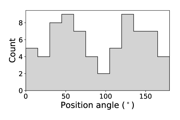
(a) Unweighted

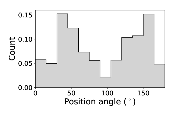
(b) Weighted

Figure 2: LQG position angles, all parallel transported to and measured at the centre of the A1 region (Hutsemékers, 1998). 2(a) is unweighted and 2(b) is ODR goodness-of-fit weighted, both with $15^{\circ}$ bins. The bimodal distribution is robust to whether or not ODR goodness-of-fit weighting is used.

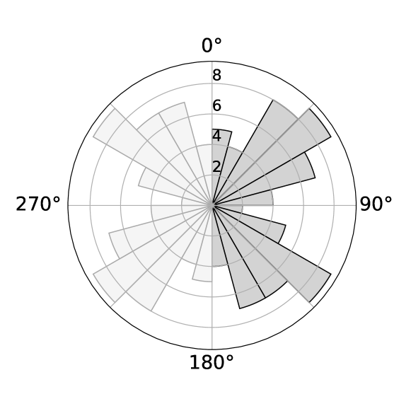
(a) Unweighted

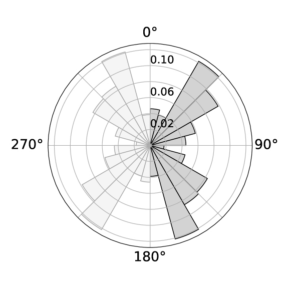
(b) Weighted

Figure 3: As Fig. 2 but represented as a rose diagram; again 3(a) is unweighted and 3(b) is ODR goodness-of-fit weighted, both with $15^{\circ}$ bins. As is conventional for undirected axial data the [$0^{\circ}$, $180^{\circ}$) data are duplicated on the opposite side of the rose diagram [$180^{\circ}$, $360^{\circ}$). For clarity, we reiterate that the PA data are axial [$0^{\circ}$, $180^{\circ}$) and not circular [$0^{\circ}$, $360^{\circ}$); we do not have PAs in the range [$180^{\circ}$, $360^{\circ}$) (the lighter shade).

We identify 71 LQGs of $\geq 20$ quasars and detection significance $\geq 2.8\sigma$. The LQG positions on the celestial sphere, and their orientation as determined by the two-dimensional method, are illustrated in Fig. 1. By eye it appears that the orientations may be somewhat preferentially aligned, but we caution that the orthographic projection may be deceiving. LQG positions in three-dimensional proper space, and their orientations, as determined by the three-dimensional method, are illustrated in Appendix G.

The results of both the 2D and 3D approaches are presented in Tables 1 (example LQGs) and 4 (full LQG sample, Appendix C.2), and generally agree well. The PAs listed in these tables are measured in situ at the location of each LQG, and will have parallel transport corrections applied before statistical analysis (section 5). For both approaches, bootstrap re-sampling with replacement is used to estimate the uncertainty in the form of the half-width confidence interval (HWCI, $\gamma_{h}$) of 10000 bootstraps.

Figs. 2 (histograms) and 3 (rose diagrams) show LQG PAs, after parallel transport, both unweighted and weighted by orthogonal distance regression goodness-of-fit (Eq. 1). For axial data [$0^{\circ}$, $180^{\circ}$), where $0^{\circ}$ and $180^{\circ}$ are equivalent, a conventional histogram (Fig. 2) can be misleading, since it represents data that are close together (e.g. $1^{\circ}$ and $179^{\circ}$) at opposite extremes of the distribution. An alternative representation is the rose diagram (Fig. 3), where wedge length is proportional to the count and spanning angle denotes the bins.

In both Figs. 2 and 3 the data appear bimodal, with peaks at $\theta\sim 45^{\circ}$ and $\theta\sim 135^{\circ}$ (in the absence of goodness-of-fit weighting). The peaks are separated by $\Delta\theta\sim 90^{\circ}$, indicating that some LQGs may have PAs that are preferentially parallel (i.e. aligned) while others are preferentially orthogonal to one another (this is described as ‘anti-aligned’ by Hutsemékers et al. (2014) and Pelgrims (2016)).

4.1 LQG PAs as a function of redshift

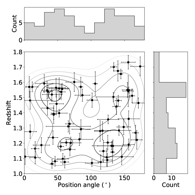
Figure 4: Marginal plot of the LQG PA $\times$ redshift plane. Error bars are PA half-width confidence interval and redshift standard deviation. Marginal histograms show PA and redshift distributions with $\Delta\theta=15^{\circ}$ and $\Delta z=0.1$ bins. Contours are a Gaussian kernel density estimation of the scatter plot. Histograms and KDE are unweighted.

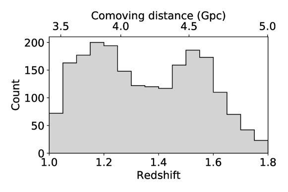
Figure 5: Redshift distribution of the 2076 member quasars comprising our sample of 71 LQGs, with $\Delta z=0.05$ bins, unweighted. Top x-axis shows approximate proper radial distance. Distribution is bimodal, with modes (peaks) at $z\sim 1.15$ and $z\sim 1.55$.

Fig. 4 shows a marginal plot of the LQG PA $\times$ redshift plane; redshift here is LQG redshift, defined as the mean redshift of its member quasars. From Fig. 2(a), we expect the PA histogram (top margin) to be bimodal, as seen. The redshift histogram (right margin) also exhibits some bimodality. To investigate the relationship between these two variables, and whether there is any correlation between their modes, we add kernel density estimation (KDE) contours to the scatter plot. This shows hints of three or four modes, although the correlation is weak. We note that the apparently stronger modes at $\theta\sim 45^{\circ}$ $\times$ $z\sim 1.5$ and $\theta\sim 135^{\circ}$ $\times$ $z\sim 1.2$ result from the points with the greatest uncertainty. Conversely, the weaker modes at $\theta\sim 55^{\circ}$ $\times$ $z\sim 1.2$ and $\theta\sim 150^{\circ}$ $\times$ $z\sim 1.5$ result from the points with the smallest uncertainty.

Due to their scale, LQGs extend considerably in the radial direction, and some features may be lost when we analyse only their mean redshift. Our sample of 71 LQGs collectively comprise 2076 member quasars. Fig. 5 shows the redshift distribution of these. The distribution appears bimodal with modes (peaks) at $z\sim 1.15$ and $z\sim 1.55$, similar to that for LQG redshifts (Fig. 4, right margin).

4.2 LQG PA weights

(a) ODR GoF weighted

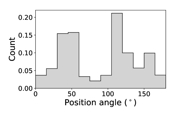
(b) HWCI weighted

Figure 6: Position angles calculated by 2D approach, with no parallel transport, and $15^{\circ}$ bins. 6(a) is goodness-of-fit weighted and 6(b) is half-width confidence interval weighted. The bimodal distribution is robust to which method of weighting is used.

The two-dimensional approach of determining position angles uses orthogonal distance regression (ODR) of tangent plane projected quasars. We evaluate the ODR goodness-of-fit (Eq. 1), which may be used to weight the PAs used for some of the statistical analysis (section 5). An alternative empirical weighting scheme could use measurement uncertainties, or half-width confidence intervals (HWCIs, Appendix E), estimated from 10000 bootstraps.

The PA distribution is robust between these alternative weighting schemes. Fig. 6 shows PAs, determined by the 2D approach, with no parallel transport, and weighted by 6(a) goodness-of-fit weights $w=\ell/\sigma^{2}$, and 6(b) HWCI weights $w=1/\gamma_{h}$. The bimodal distribution is robust to which method of weighting is used. We continue to use the former in this work as it is more physically motivated and slightly more conservative.

5 Results: statistical analysis

The position angle distribution of our sample of 71 LQGs appears bimodal, with modes at $\bar{\theta}\sim 52\pm 2^{\circ},137\pm 3^{\circ}$ (with goodness-of-fit weighting) after parallel transport to the centre of the A1 region (Hutsemékers, 1998). The median location of the peaks after parallel transport to all 71 LQG locations is $\bar{\theta}\sim 45\pm 2^{\circ},136\pm 2^{\circ}$. The peaks are separated by $\Delta\theta\sim 90^{\circ}$, indicating that some LQGs have PAs that are preferentially aligned with each other, while others are preferentially orthogonal. We apply the statistical methods of section 3 to analyse the uniformity, bimodality, and correlation of these PAs.

5.1 Uniformity: LQG PAs are unlikely to be uniform

Table 2: Results ($p$-values) of uniformity tests. For 2-axial (4-axial) PAs the $\chi^{2}$ test is evaluated using $20^{\circ}$ ($10^{\circ}$) bins. The $\chi^{2}$ and Kuiper’s tests are computed both with and without goodness-of-fit weighting. For 2-axial PAs, only the $\chi^{2}$ test shows evidence for non-uniformity (of weighted PAs). For 4-axial PAs, all tests show evidence for non-uniformity, mostly marginal, with Kuiper’s being the most significant.

	$p$-value
	2-axial		4-axial
test	unweighted	weighted	unweighted	weighted
$\chi^{2}$	0.16	0.01	0.07	0.02
Kuiper’s	0.62	0.59	0.009	0.008
HR	0.07	-	0.04	-

The results from applying the uniformity tests are listed in Table 2. The $\chi^{2}$ test does not show evidence of non-uniformity for 2-axial PAs without weighting ($16\%$ significance level), but does show some evidence of non-uniformity with weighting ($1\%$ significance level). For 4-axial PAs it shows marginal evidence of non-uniformity both with and without weighting ($2\%$ and $7\%$ respectively).

Kuiper’s test does not show evidence of non-uniformity for 2-axial PAs, with or without weighting. However, the PA distribution is bimodal, which dramatically reduces the test’s discriminatory power, so the absence of a signal is unsurprising. For 4-axial PAs Kuiper’s test indicates a rejection of the null hypothesis of uniformity at the $0.8\%$ and $0.9\%$ significance level (weighted and unweighted), i.e. $\sim 2.4\sigma$.

Finally, the Hermans-Rasson test shows marginal evidence of non-uniformity for 2-axial and 4-axial PAs ($7\%$ and $4\%$ significance levels, respectively), both without weighting.

Based on the results from these three uniformity tests we cannot confidently reject the null hypothesis that the observed PAs are drawn from a uniform distribution. The most appropriate test for the axial and bimodal nature of the 2-axial PA data is the HR test, which shows marginal evidence of non-uniformity.

However, if we a priori expect f-fold symmetry (specifically 2-fold, in case of a bimodal distribution) then the conversion of PAs to 4-axial becomes physically well motivated as well as statistically legitimate. In this case, based on the 4-axial results of Kuiper’s test, we could confidently reject the null hypothesis and conclude that the PAs are non-uniform.

5.1.1 Uniformity of mock LQG catalogues

Table 3: Results ($p$-values) of uniformity tests applied to mock LQGs. For 2-axial (4-axial) PAs the $\chi^{2}$ test is evaluated using $15^{\circ}$ ($7.5^{\circ}$) bins, except for individual mocks where it is evaluated using $30^{\circ}$ ($15^{\circ}$) bins. For multiple samples the number of LQGs and $p$-values are means plus the standard error on the mean. All PAs are unweighted and are parallel transported to, and measured at, the centre of the Al region (Hutsemékers, 1998). Most samples and tests show no evidence for non-uniformity.

	No. of		$p$-value
sample(s)	LQGs	test	2-axial	4-axial
110	$30\pm 0.4$	$\chi^{2}$	$0.53\pm 0.03$	$0.51\pm 0.03$
individual		Kuiper’s	$0.53\pm 0.03$	$0.50\pm 0.03$
mocks		HR	$0.48\pm 0.03$	$0.50\pm 0.03$
10 stacks	$330\pm 3$	$\chi^{2}$	$0.47\pm 0.10$	$0.41\pm 0.08$
of 11		Kuiper’s	$0.56\pm 0.10$	$0.44\pm 0.09$
sub-volumes		HR	$0.46\pm 0.11$	$0.62\pm 0.09$
1 stack	3,296	$\chi^{2}$	0.20	0.31
of		Kuiper’s	0.27	0.03
110 mocks		HR	0.16	0.15

The results from applying uniformity tests to the mock LQGs of section 2.4 are listed in Table 3. The $\chi^{2}$ and Hermans-Rasson tests show no evidence for non-uniformity of the mock LQGs. This result is consistent between 2 and 4-axial PAs, individual mocks, stacks of sub-volumes, and the stack of all 3,296 mock LQGs.

Kuiper’s test also shows no evidence for non-uniformity, except for the stack of all mock LQGs evaluated as 4-axial data (and then only marginally). This could be an artefact of the realizations not being truly independent, but if so it is unclear why this would reveal itself only in one of the six tests on this sample. Our concerns about the independence of this particular stack, the otherwise highly consistent results, and our caution about interpreting results manifest only in 4-axial data, led to this anomalous result being discredited. We therefore conclude that all three tests indicate statistical uniformity of the mock LQGs.

5.2 Bimodality: LQG PA distribution is bimodal

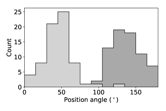
Figure 7: Location of the centres of the double Gaussian peaks in Fig. 19; $15^{\circ}$ bins. The locations of the two peaks are consistent, regardless of parallel transport destination. The mean locations are $\sim 47\pm 2^{\circ}$ and $\sim 138\pm 2^{\circ}$, consistent (within $\lesssim 10^{\circ}$) with the HDS result.

We calculate Hartigans’ dip statistic (HDS) for continuous unweighted PA data and recover two peaks between $\sim 36^{\circ}-83^{\circ}$ and $\sim 114^{\circ}-156^{\circ}$, with 97% confidence. The unweighted (weighted) means of PAs in these two ranges are $\sim 54\pm 2^{\circ}$ ($\sim 52\pm 2^{\circ}$) and $\sim 136\pm 3^{\circ}$ ($\sim 137\pm 3^{\circ}$), consistent with the peaks we see in the distribution of categorical PA data (e.g. Fig. 2). The bimodality is therefore unlikely to be an artefact of binning.

We apply HDS after all PAs are parallel transported to the centre of the A1 region. Recalling section 2.3 (see also Jain et al., 2004), the process of parallel transport rotates PAs; the amount of rotation depending on the path taken (direction and distance). Therefore it is reasonable to check whether parallel transporting to a different location would affect the position of the PA peaks.

We parallel transport all 71 PAs to the location of each of the 71 LQGs, and at each one fit a double Gaussian to the unweighted histogram of these PAs. The height, width, and location of each Gaussian are fitted using Python’s scipy.optimize.leastsq.

The location of the centres of the double Gaussian peaks, at each of the 71 LQG locations, are shown in Fig. 7. The median (mean) location of the first peak is $\sim 45\pm 2^{\circ}$ ($\sim 47\pm 2^{\circ}$), and of the second is $\sim 136\pm 2^{\circ}$ ($\sim 138\pm 2^{\circ}$). These are consistent (within the mean PA half-width confidence interval of $\sim 10^{\circ}$) with the peaks identified by HDS at the centre of the A1 region ($\sim 54\pm 2^{\circ}$ and $\sim 136\pm 3^{\circ}$ for unweighted PAs).

Individual PA distributions at each of the 71 LQG locations are shown in Fig. 19 (Appendix H). At most ($\gtrsim 80\%$) the PAs show a similar bimodal distribution.

5.3 Correlation: LQG PAs are aligned and orthogonal

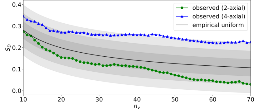
Figure 8: The S test statistic $S_{D}$ calculated for 2-axial (green circles) and 4-axial (blue triangles) PAs as a function of nearest neighbours $n_{v}$ determined in 3D. Also shown, empirical values estimated for a uniform distribution (black) and their approximate $\pm 1\sigma,\ 2\sigma,\ 3\sigma$ confidence intervals (grey). 4-axial PAs show more alignment than uniform, while 2-axial show less.

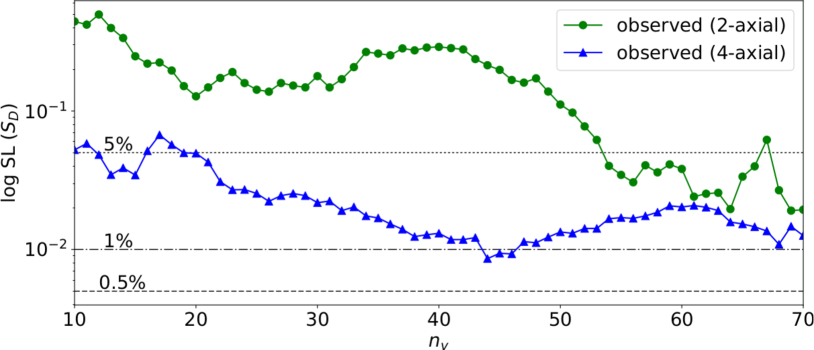
Figure 9: The logarithmic significance level (SL) of the S test calculated for 2-axial (green circles) and 4-axial (blue triangles) PAs as a function of nearest neighbours $n_{v}$ determined in 3D. The dotted, dash-dotted and dashed horizontal lines indicate SL = 0.05, 0.01 and 0.005 respectively. 2-axial LQG PAs show correlation ($\mathrm{\overline{SL}}\sim 3.3\%$) above $n_{v}\geq 54$. 4-axial PAs show correlation ($\mathrm{\overline{SL}}\sim 1.5\%$) above $n_{v}\geq 30$.

We compute the S statistic $S_{D}$ using the Jain et al. (2004) coordinate invariant version of the S test for samples of $n_{v}$ nearest neighbours, where $10\leq n_{v}\leq 70$. In Fig. 8 we show the values of $S_{D}$ calculated for observed LQG PAs, represented as both 2-axial (green circles) and 4-axial (blue triangles) data, as a function of nearest neighbours $n_{v}$. Nearest neighbours are determined in 3D, taking into account radial distance. Results are entirely consistent with neighbours determined in 2D (i.e. by angular separation).

Larger values of $S_{D}$ indicate stronger alignment. So Fig. 8 indicates that 4-axial LQG PAs are more aligned than expected if they are randomly drawn from a uniform distribution. Conversely, it also suggests that 2-axial LQG PAs are less aligned (or more orthogonal) than expected. The physical interpretation of the latter is not straightforward, but likely to be due to the contribution from orthogonal PAs leading to large dispersion, and hence a small value of $S_{D}$.

The approximate empirical standard deviation, and hence the $\pm 1\sigma,2\sigma$, and $3\sigma$ confidence intervals shown in Fig. 8, are valid only for large $n$ while $n_{v}\ll n$ (Jain et al., 2004). These are not valid assumptions for much of our range of $S_{D}$. Therefore, due to this and the mutual dependence between groups of nearest neighbours, we calculate the significance level of the S test using numerical simulations. In Fig. 9 we show the significance level of the S test calculated using 10000 numerical simulations, for values of $S_{D}$ determined using both 2-axial (green circles) and 4-axial (blue triangles) PAs. Again, this is shown as a function of nearest neighbours $n_{v}$.

With 4-axial LQG PAs we test for alignment and orthogonality by combining the modes, resulting in an alignment only signal (right-hand $S_{D}$ tail). We find significance levels generally between 1% and 5% for most numbers of nearest neighbours $n_{v}$. For most of the $n_{v}$ range ($30\leq n_{v}\leq 70$) the significance level is $0.9\%\leq\mathrm{SL}\leq 2.2\%$, with a mean (median) of 1.5% (1.5%). It is most significant for $n_{v}\sim 45$, with $\mathrm{SL}\simeq 0.8\%$.

For 2-axial LQG PAs the orthogonal mode appears to dominate (left-hand $S_{D}$ tail). We find significance levels generally above 5% until $n_{v}\geq 54$. For the remainder of the range of $n_{v}$ ($54\leq n_{v}\leq 70$) the SL is $1.9\%\leq\mathrm{SL}\leq 6.2\%$, with a mean (median) of 3.3% (3.4%).

5.3.1 Typical angular and proper separations

The number of LQG nearest neighbours $n_{v}$ is a free parameter explored by the S test. We identify these neighbours using the three-dimensional proper positions of each LQG centroid. The parameter $n_{v}$ is related to the scale of the nearest neighbour groups, but because LQGs are not homogeneously distributed we cannot directly interpret it as corresponding to a particular scale. We evaluate the relationship between the parameter $n_{v}$ and the typical scale of the nearest neighbour groups, defined as the median separation between each LQG and its $n_{v}$ nearest neighbours.

Using these relationships, we evaluate the S test significance levels as a function of typical separation instead of nearest neighbours $n_{v}$. The functions do not differ significantly in shape, because the relationships are generally linear when $n_{v}\gtrsim 20$. We find that the correlation is most significant for typical angular (proper) separations of $\sim 30^{\circ}$ (1.6 Gpc).

6 Discussion and conclusions

We find that LQG PAs are unlikely to be drawn from a uniform distribution ($p$-values $0.008\lesssim p\lesssim 0.07$). However, similar non-uniformity is not found in mock LQG catalogues, indicating the LQG correlation is not found in cosmological simulations. Further, the LQG PA distribution is bimodal, with modes for weighted PAs at $\bar{\theta}\sim 52\pm 2^{\circ},137\pm 3^{\circ}$ (97% confidence). This bimodality is robust to parallel transport destination, with the median location of the peaks at all 71 LQG locations of $\bar{\theta}\sim 45\pm 2^{\circ},136\pm 2^{\circ}$. These angles are remarkably close to the mean angles of radio quasar polarisation of $\bar{\theta}\simeq 42^{\circ}$ and $\bar{\theta}\simeq 131^{\circ}$, reported by Pelgrims & Hutsemékers (2015) in two regions coincident with our LQG sample.

LQGs are aligned and orthogonal across very large scales, with a maximum significance of $\simeq 0.8\%$ ($2.4\sigma$) for groups of $\sim 45$ nearest neighbours, corresponding to typical angular (proper) separations of $\sim 30^{\circ}$ (1.6 Gpc). The statistical significance of this correlation is marginal, therefore we cannot exclude it being a chance statistical anomaly. However, its coincidence with regions of quasar-polarisation alignment (e.g. Hutsemékers, 1998; Pelgrims & Hutsemékers, 2015), the link between quasar polarisation and LQG axes (Hutsemékers et al., 2014; Pelgrims & Hutsemékers, 2016), and the similarity between LQG position angles and the preferred angles of quasar radio polarisation alignment (Pelgrims & Hutsemékers, 2015), suggest an interesting result.

We find no indication that boundary effects or selection effects have influenced these results. Three of the LQGs might be truncated by the RA, Dec. boundaries of DR7QSO: removing them from consideration made no significant difference. Randomly-generated LQGs with related parameters (same encompassing circle, same number of members) to the real LQGs did not reproduce the results.

A plausible mechanism for the correlation of LQG orientations on such large scales is not obvious. We considered the geometry of the Universe. van de Weygaert (2007) uses Voronoi tessellation (Voronoï, 1908) to describe the observed cosmic web on $\gtrsim 100$ Mpc scales (see also Icke & van de Weygaert, 1987; van de Weygaert, 1994). We speculated whether a cellular structure to the Universe, such as Voronoi tessellation, or a more regular crystalline structure, could cause such an effect.

We also considered primordial anisotropies. Poltis & Stojkovic (2010) proposed cosmic strings as an explanation for quasar-polarisation alignments. They suggest the decay of these would seed correlated primordial magnetic fields. However, using the CMB, the possible amplitude of these has been constrained to less than a few nanoGauss (Planck Collaboration et al., 2016). Hutsemékers et al. (2005) suggest the apparent rotation of mean optical quasar polarisation angle with redshift may be caused by a global rotation of the Universe, such as that invoked by Jaffe et al. (2005) to explain large-scale anisotropies in the CMB data. However, from CMB temperature and polarisation analysis Saadeh et al. (2016) conclude that the Universe is neither rotating nor anisotropically stretched.

For the geometric and primordial explanations we considered, it is unclear how they could translate into our observed position angle distribution. Further, the primordial explanations have been disfavoured by observations. The origin of the LQG orientation correlation remains unexplained.

We found no evidence of $\Lambda$CDM cosmological simulations predicting correlations between objects on Gpc scales, but this had not been specifically examined for LQGs. Using mock LQG catalogues (Marinello et al., 2016) we found no evidence of LQG correlation in the Horizon Run 2 simulation (Kim et al., 2011). This suggests that the cosmic web of the observed Universe differs on the largest scales to this dark-matter-only $N$-body simulation. It hints that there could, given the caveats associated with the simulations, be aspects of the large-scale structure that are not captured by the power spectrum. Running the LQG finder on other cosmological simulations would be informative. If the correlation in LQG orientation is confirmed then perhaps it is an unexpected feature of known physics. If it is not seen then perhaps something is missing from the simulations (e.g. primordial anisotropies) or it is, after all, a statistical fluke which coincidentally gives rise to the aligned quasar polarisations.

The LQG orientation correlation we found offers a plausible explanation for the quasar-polarisation alignments reported by many studies (e.g. Hutsemékers, 1998; Hutsemékers & Lamy, 2001; Jain et al., 2004; Cabanac et al., 2005; Tiwari & Jain, 2013; Pelgrims & Cudell, 2014; Pelgrims & Hutsemékers, 2015; Pelgrims, 2019). If LQG axes are preferentially aligned at $\bar{\theta}\sim 45\pm 2^{\circ},136\pm 2^{\circ}$ (this work, median modes), and if quasar polarisation vectors are preferentially parallel and orthogonal to LQG axes (Hutsemékers et al., 2014; Pelgrims & Hutsemékers, 2016), this could result in polarisation vectors with preferred angles of $\sim 42^{\circ}$ and $\sim 131^{\circ}$ (Pelgrims & Hutsemékers, 2015). Our results therefore offer corroborating evidence for, and enhancement of, the intrinsic alignment interpretation of these studies.

Quasar-polarisation alignment is also detected in the south Galactic cap (SGC, e.g. Hutsemékers, 1998; Pelgrims & Hutsemékers, 2015), which is not coincident with our LQG sample in the north Galactic cap (NGC). The forthcoming 4-metre Multi-Object Spectroscopic Telescope (4MOST) Active Galactic Nuclei survey (Merloni et al., 2019) will survey a million $z\lesssim 2.5$ quasars over $\sim 10000\ \mathrm{deg}^{2}$, with first light expected in 2022. This could deliver an LQG sample in the SGC for similar evaluation to our work in the NGC. Of particular interest would be whether LQG orientation again corresponds to the preferred angle of quasar radio polarisation alignment, which differ between NGC and SGC (e.g. Pelgrims, 2016).

Our results are based on a sample of 71 LQGs at redshifts $1.0\leq z\leq 1.8$, which were detected using the SDSS DR7QSO catalogue (Schneider et al., 2010) of $\sim 105$k quasars across $\sim 7600\ \mathrm{deg}^{2}$. Forthcoming spectroscopic surveys will deliver a far larger sample of quasars, e.g. the Dark Energy Spectroscopic Instrument (DESI, DESI Collaboration et al., 2016) 5-year survey aims to target 1.7 million $z<2.1$ quasars covering $\sim 14000\ \mathrm{deg}^{2}$, beginning in May 2021. This has the potential to deliver a larger sample of LQGs for a better assessment of their correlation.

If the LQG orientation correlation is real, it represents large-scale structure alignment over $\gtrsim$ Gpc scales, larger than those predicted by cosmological simulations and at least an order of magnitude larger than any so far observed, with the exception of quasar-polarisation / radio-jet alignment. Careful statistical analysis is required before making inferences about whether such a large-scale correlation challenges the assumption of large-scale statistical isotropy and homogeneity of the Universe.

To conclude, we find large-scale correlation of LQG orientations, which we report here for the first time. This helps explain a substantial body of work on quasar-polarisation / radio-jet alignment, but at the expense of raising potentially even more challenging questions about the origin of the LQG correlation and its implications for isotropy and homogeneity. Forthcoming surveys and the other future work we suggest here will illuminate LQGs and their intriguing correlation further.

Data availability statement

The datasets were derived from sources in the public domain: https://classic.sdss.org/dr7/products/value_added/qsocat_dr7.html.

Appendix A LQG finder

Clowes et al. (2012, 2013) detect LQG candidates using a three-dimensional single-linkage hierarchical clustering algorithm, also known as friends-of-friends (FoF). This is equivalent to a three-dimensional minimal spanning tree (MST). These type of methods are widely used to detect galaxy clusters, superclusters, voids, and filaments (e.g. Press & Davis, 1982; Einasto et al., 1997; Park et al., 2012; Pereyra et al., 2020), as well as LQGs (e.g. Clowes et al., 2012, 2013; Nadathur, 2013; Einasto et al., 2014; Park et al., 2015). They make no assumptions about cluster morphology.

Using the terminology of Barrow et al. (1985), MST treats the dataset as a graph made up of vertices (nodes, in this case quasars) which are connected by edges (straight lines). This is a ‘tree’ when it has no closed paths (sequence of edges) and a ‘spanning’ tree when it contains all the vertices. For any graph, there are multiple possible spanning trees; the ‘minimal’ spanning tree is that of minimal length (sum of edge lengths). To identify clusters within the MST it may be separated, where edges exceeding a certain length are removed, leaving groups of objects with mutual separations less than this ‘linkage length’.

The choice of linkage length is crucial - too long and clusters merge to fill the entire volume, too short they break up into pairs and triplets (Graham et al., 1995). Pilipenko (2007) categorises the criteria for making this choice as physical or formal. With a priori knowledge of physical parameters (e.g. size, membership, density) of the clusters, it is possible to choose the scale that maximises the fraction of clusters with those parameters. The criterion used by Graham et al. (1995) is an example of a physical approach; they choose the scale that maximises the number of clusters of a minimum membership. An example formal approach would be to choose a scale based on the mean nearest-neighbour separation.

Clowes et al. (2012, 2013) use this latter approach. Their quasar sample has a mean nearest-neighbour separation of $\sim 74\ \mathrm{Mpc}$. They also account for uncertainties in their edge lengths (i.e. proper distances) due to redshift errors and peculiar velocities (for estimates, see Clowes et al., 2012) and choose a linkage length of $100\ \mathrm{Mpc}$.

Clowes et al. (2012, 2013) estimate the overdensity and statistical significance of their LQGs using a convex hull of member spheres (CHMS) method. This is described in detail in Clowes et al. (2012), but briefly, for each LQG they calculate the volume of a convex hull of spheres of radius half the mean edge length at each vertex (member quasar location). The CHMS volume of an LQG of $m$ members is then compared with the distribution of CHMS volumes of clusters of $m$ points in Monte Carlo simulations of the same size and density as their control area, in order to estimate overdensity and statistical significance. We note this method of estimating statistical significance is not universally accepted (Nadathur, 2013; Pilipenko & Malinovsky, 2013; Park et al., 2015).

The Huge-LQG and Clowes-Campusano LQG, amongst others, have been independently detected using different FoF algorithms (Nadathur, 2013; Einasto et al., 2014; Park et al., 2015). Indeed, and unsurprisingly, our LQG sample has many objects in common with the publicly available catalogue of Einasto et al. (2014). Einasto et al. (2014) appear to have followed closely the approach of Clowes et al. (2012, 2013) in terms of input data, selection algorithm, linkage scale, and cosmological model and parameters, but applied to a reduced area of DR7QSO. Einasto et al. (2014) differed substantially, however, in not providing any measures of statistical significance or overdensity, which are important for ranking the LQG candidates.

Appendix B LQG sample

Fig. 10 illustrates the 71 LQGs in our sample, shown in tangent plane projection.

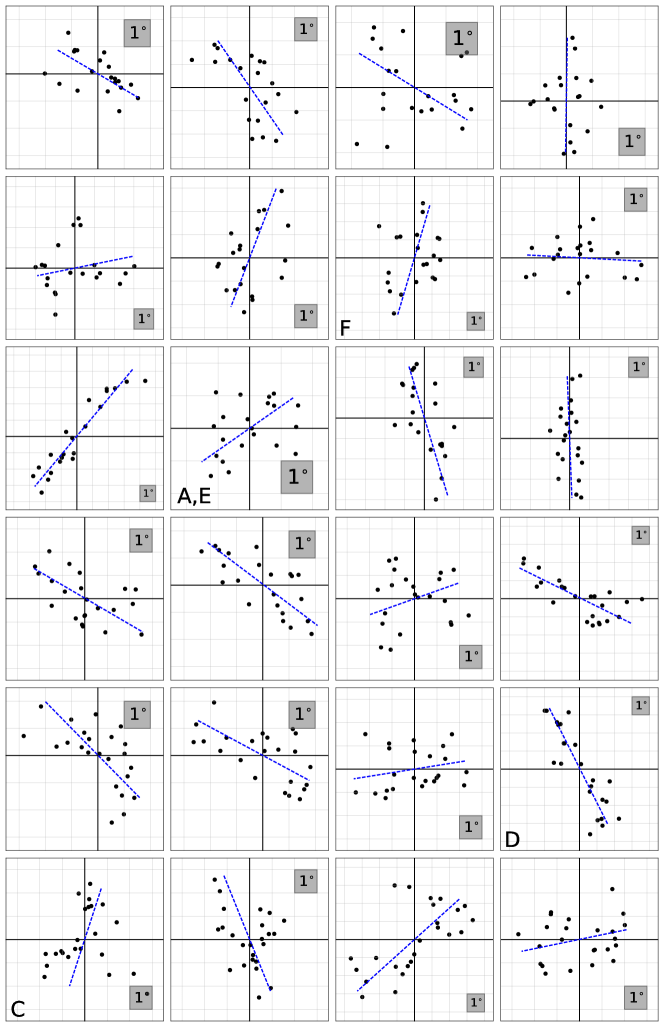
Figure 10: (a) Tangent plane projection of 1-24 (across then down) of the 71 LQGs in our sample, in Cartesian coordinates. Member quasars shown as black dots, orthogonal distance regression fit shown as dashed blue line. Solid black lines indicate $x=0$ and $y=0$, and grey square illustrates scale ($1^{\circ}$). LQGs labelled A, C (D, E, F) are discussed in Fig. 15 (Fig. 16).

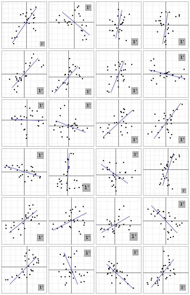
Figure 11: (b) Tangent plane projection of 25-48 (across then down) of the 71 LQGs in our sample, in Cartesian coordinates. Other plot details are as for Fig. 10 panel (a).

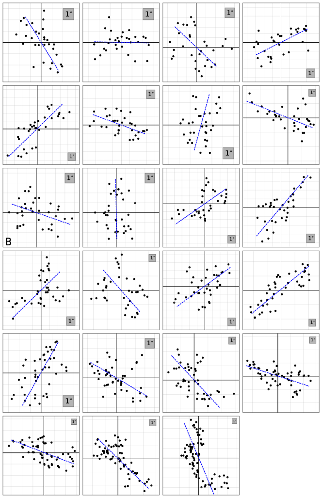
Figure 12: (c) Tangent plane projection of 49-71 (across then down) of the 71 LQGs in our sample, in Cartesian coordinates. Other plot details are as for Fig. 10 panel (a). LQG labelled B is discussed in Fig. 15.

Appendix C LQG orientation

C.1 LQG position angles — presentation

The position angle (PA) of a large quasar group can be calculated in either two or three dimensions. In two dimensions we treat the quasars as points on the celestial sphere, whereas in three dimensions we take into account their proper radial distances.

For the 2D approach quasar positions (in right ascension and declination) are projected onto the tangent plane as Cartesian $(x,y)$ points. This plane meets the celestial sphere at the centre of gravity of the LQG $(x,y)=(0,0)$, calculated assuming quasars are point-like unit masses. To determine LQG orientation we use orthogonal distance regression (ODR) of these projected points (see Fig. 13 for an example). This minimises the sum of the squares of the orthogonal residuals between the points and the line (for a discussion of OLS, ODR, and other regression methods, see Isobe et al., 1990).

For the 3D approach the covariance matrix of the quasar proper positions is decomposed into its eigenvectors and eigenvalues. Again, quasars are assumed to be point-like unit masses. The axes of a confidence ellipsoid (e.g. Fig. 14) are constructed from the eigenvectors and eigenvalues; each axis is in the direction of its eigenvector and its length $\ell$ is a function of its eigenvalue $\lambda$, specifically $\ell\propto\sqrt{\lambda}$. The first principal component (ellipsoid major axis) is given by the eigenvector with the largest eigenvalue. Finally, this is projected onto the plane orthogonal to the line-of-sight to define the (2D projected) PA.

PAs determined by the two approaches may differ, for example the 2D approach may be susceptible to projection effects and the 3D approach may be susceptible to redshift-space distortions. The orientation of the LQG with respect to the line-of-sight and its morphology may also induce differences. We expect PAs determined by the two approaches to agree well when the LQG is linear and orthogonal to the line-of-sight, but they may differ significantly when the LQG is broad, crooked, curved or aligned along the line-of-sight.

For our sample of 71 LQGs we find that the two approaches are generally consistent. Fig. 15 shows the PAs calculated using both the 2D and 3D approaches. Note that the PAs have not been parallel transported, but these angles serve as a useful comparison between the two approaches. The error bars are the half-width confidence intervals estimated using bootstrap re-sampling. Note that, usually, the measurement uncertainties are slightly larger for the 3D approach.

The three widest outliers from the 1:1 diagonal line in Fig. 15 are due to the geometry of these particular LQGs (A, B, C; also labelled in Fig. 10). Two of these LQGs (A and B) have their major axes oriented towards the line-of-sight, and not significantly longer than their first minor axes. Indeed, for both of these, the 2D approach fits a regression comparable to the first minor axes rather than the major axes. One LQG (C) is very irregular so linear fits are poor, and corresponding PAs are uncertain, in both the 2D and 3D approaches. The PAs of all three of these LQGs are given little weight by goodness-of-fit weighting (section 2.2).

Both the 2D and 3D approaches have been used to determine the PAs of LQGs. Hutsemékers et al. (2014) use the 2D approach to demonstrate alignment of quasars’ optical linear polarisation with LQG axes, while Pelgrims & Hutsemékers (2016) use the 3D approach to evidence alignment of quasars’ radio polarisation with more LQG axes. The latter derived eigenvectors and eigenvalues from the inertia tensor rather than covariance matrix; results are equivalent. Pelgrims & Hutsemékers (2016) report that for the 2D approach PAs calculated using ODR are consistent (within $1^{\circ}$) with those determined using the inertia tensor.

Pelgrims & Hutsemékers (2016) show that both approaches usually agree well, and argue that the 3D approach is more physically motivated. We agree, but note that any 3D analysis is susceptible to redshift errors. The quasars in our sample are from SDSS DR7QSO, which typically has quoted redshift errors of $\Delta z\sim 0.004$ (Schneider et al., 2010). There is also evidence for systematic errors of $\Delta z\sim 0.003$ (Hewett & Wild, 2010). Using Monte Carlo simulations we find that these redshift errors introduce uncertainty in the PA, generally of a few degrees, but up to $\sim 30^{\circ}$ for LQGs particularly oriented along the line-of-sight (e.g. LQGs A and B).

Furthermore, in the 3D approach, there is also the potential for errors due to redshift-space distortions from the quasars’ peculiar velocities, causing their real-space distribution to be either elongated (Jackson, 1972) or squashed (Kaiser, 1987) along the line-of-sight. We find that the measurement uncertainties (Appendix E) are slightly larger for the 3D approach. We therefore base our analysis on the two-dimensional approach; tangent plane projection of the LQG and orthogonal distance regression of the projected quasars.

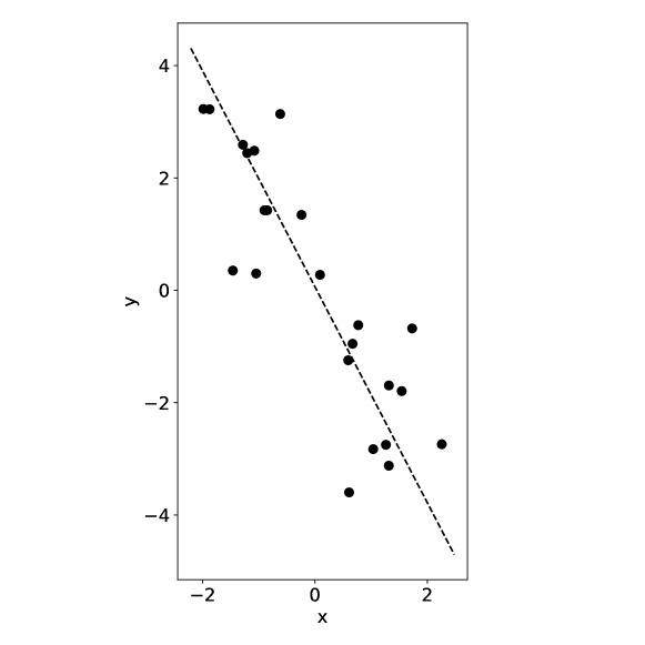
Figure 13: Tangent plane projection of an LQG, with coordinates ($\alpha$, $\delta$) projected to ($x$, $y$). Member quasars are shown as black dots and orthogonal distance regression fit shown as dashed line. Axes are labelled in degrees. This LQG is also shown in Figs. 10 and 16, labelled D. Using the 2D PA approach, PA = $152.5^{\circ}$.

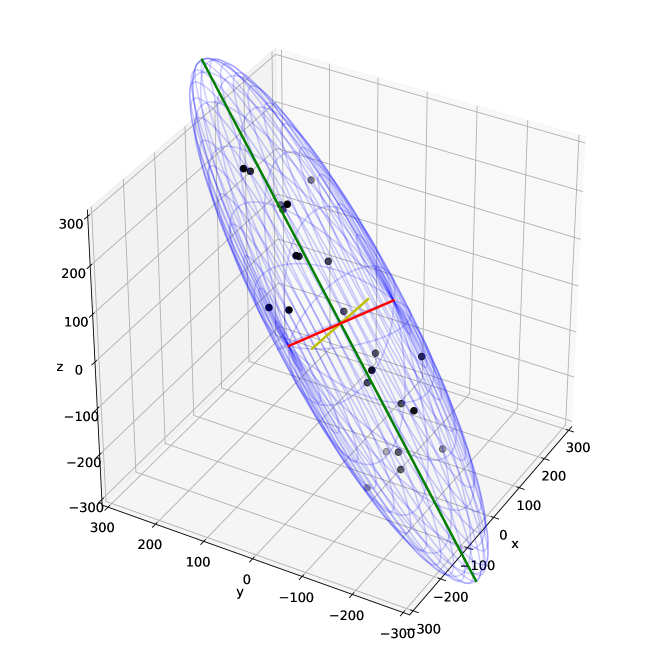
Figure 14: Same LQG as Fig. 13, but shown in 3D proper coordinates oriented with line-of-sight orthogonal to the page. Axes of enclosing ellipsoid (green = a-axis, yellow = b-axis, red = c-axis) constructed from eigenvectors and eigenvalues. Axes are labelled in Mpc. Using the 3D PA approach, 2D projected PA = $152.3^{\circ}$.

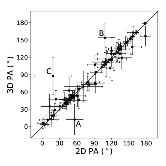
Figure 15: Position angles of 71 LQGs calculated by 2D and 3D approaches. The two generally agree well, with the three widest outliers (A, B, C) due to the geometry of those particular LQGs (see text and Fig. 10). Error bars show half-width confidence intervals estimated using bootstrap re-sampling.

C.2 LQG position angles — tabulation

Table 4 presents the results of both the two-dimensional and three-dimensional approaches to determining position angle. To recap, the 2D approach involves tangent plane projection of the LQG quasars, followed by orthogonal distance regression (ODR) of the projected points. The 3D approach requires determining the proper coordinates of the LQG quasars, performing principal component analysis on the covariance matrix of these, then tangent plane projection of the resultant major axis.

The results of both approaches generally agree well. For both approaches, bootstrap re-sampling with replacement is used to estimate the uncertainty in the form of the half-width confidence interval (HWCI, $\gamma_{h}$) of 10000 bootstraps. The PAs listed in Table 4 are measured in situ at the location of each LQG, and will have parallel transport corrections applied before statistical analysis.

Table 4: The 71 large quasar groups, where $m$ is the number of members, and $\bar{\alpha}$, $\bar{\delta}$, and $\bar{z}$ are the mean right ascension, declination, and redshift of the member quasars. The normalized goodness-of-fit weight $w$ (Eq. 1) is scaled by $w_{71}=w\times 71$ for clarity, and to distinguish those LQGs weighted higher ($w_{71}>1$) or lower ($w_{71}<1$) than the mean $\bar{w}$. Position angle $\theta$ and half-width confidence interval $\gamma_{h}$ are shown for both the 2D and 3D approaches. The ratio of LQG ellipsoid axes lengths (from the 3D approach, Appendix C) is given by $a:b:c$. This list was summarized in Table 1.

	J2000 (∘)				2D PA (∘)		3D PA (∘)
$m$	$\bar{\alpha}$	$\bar{\delta}$	$\bar{z}$	$w_{71}$	$\theta$	$\gamma_{h}$	$\theta$	$\gamma_{h}$	$a:b:c$
20	121.1	27.9	1.73	1.13	119.7	10.4	115.1	10.7	0.50:0.30:0.21
20	151.5	48.6	1.46	1.21	144.4	9.2	144.3	11.5	0.50:0.33:0.17
20	155.9	12.8	1.50	0.32	120.7	25.2	117.2	37.0	0.44:0.43:0.14
20	163.6	16.9	1.57	1.00	0.9	8.8	5.7	9.2	0.47:0.33:0.20
20	178.0	1.2	1.23	0.37	78.9	20.3	77.0	14.7	0.51:0.31:0.17
20	216.4	1.4	1.11	0.86	21.6	8.1	28.4	11.3	0.49:0.30:0.21
21	133.5	41.2	1.40	0.72	16.9	12.1	18.5	10.6	0.49:0.33:0.18
21	170.6	16.8	1.07	0.90	93.0	10.0	94.1	15.4	0.47:0.37:0.17
21	191.8	11.0	1.06	4.43	40.9	2.8	41.0	2.9	0.66:0.24:0.10
21	209.1	3.2	1.56	0.77	55.9	14.8	12.3	25.9	0.49:0.30:0.21
21	212.9	12.6	1.55	1.72	162.7	3.9	162.8	3.9	0.63:0.22:0.15
21	231.2	25.2	1.51	4.57	177.7	3.9	178.8	2.4	0.57:0.29:0.14
22	136.8	49.5	1.19	1.03	119.4	8.2	126.4	13.2	0.46:0.38:0.17
22	182.0	55.5	1.70	1.88	126.1	4.6	126.3	4.7	0.56:0.23:0.20
22	217.8	-0.8	1.31	0.42	71.0	33.3	69.2	27.0	0.42:0.33:0.25
23	155.9	53.5	1.48	1.79	115.6	4.8	115.8	4.8	0.60:0.22:0.19
23	166.4	37.1	1.31	0.97	134.5	10.2	126.3	15.9	0.44:0.37:0.19
23	171.3	14.0	1.20	1.57	117.5	6.4	101.2	15.7	0.48:0.37:0.15
23	180.5	6.0	1.29	1.26	81.2	13.5	72.8	11.3	0.57:0.25:0.18
23	209.5	34.3	1.65	1.99	152.5	2.8	152.3	2.8	0.68:0.17:0.15
23	214.3	31.8	1.48	0.27	18.6	32.6	87.7	32.5	0.47:0.35:0.18
24	119.1	18.6	1.28	1.06	157.3	9.6	162.8	11.1	0.46:0.32:0.23
24	139.6	2.5	1.20	0.61	48.9	6.7	49.0	6.7	0.58:0.29:0.13
24	171.1	17.6	1.52	0.83	78.7	11.2	77.0	10.3	0.50:0.28:0.22
24	179.6	65.0	1.08	0.71	35.4	3.7	35.2	3.9	0.55:0.23:0.22
24	205.0	12.0	1.36	0.61	129.2	16.1	129.2	16.6	0.46:0.33:0.20
24	217.1	33.8	1.11	0.99	12.8	15.0	34.9	21.8	0.54:0.28:0.18
24	217.1	57.5	1.70	0.75	9.8	14.3	11.6	10.3	0.52:0.28:0.20
25	142.5	31.3	1.33	1.70	42.4	6.1	41.1	7.2	0.50:0.34:0.15
25	149.5	43.7	1.16	0.81	42.3	7.8	38.9	9.9	0.45:0.35:0.20
25	186.0	3.6	1.19	0.61	23.6	12.3	47.3	15.3	0.48:0.32:0.20
25	196.7	36.5	1.48	0.64	103.1	7.7	102.9	8.6	0.47:0.33:0.20
25	231.9	43.6	1.20	0.30	91.9	15.3	75.1	16.9	0.44:0.36:0.21
26	160.3	53.5	1.18	0.33	110.6	23.2	111.5	25.1	0.38:0.34:0.28
26	171.7	24.2	1.10	0.78	48.5	8.3	47.3	8.1	0.46:0.29:0.24
26	206.0	6.5	1.43	0.75	38.1	8.7	46.7	12.0	0.46:0.36:0.18
26	224.2	61.6	1.57	1.52	106.8	3.1	106.8	4.3	0.51:0.33:0.16
26	245.6	40.3	1.55	0.58	4.2	8.0	3.5	4.7	0.49:0.26:0.25
27	184.1	52.7	1.18	0.37	124.4	28.7	125.7	28.7	0.40:0.35:0.25
27	204.0	13.7	1.16	0.98	19.6	5.8	19.9	8.2	0.50:0.36:0.13
27	221.8	52.4	1.55	1.12	52.3	7.2	54.5	6.6	0.54:0.26:0.20
27	225.5	57.3	1.52	0.54	63.3	14.4	45.6	14.6	0.45:0.37:0.18
27	231.2	15.4	1.56	1.01	60.8	14.0	53.2	18.7	0.43:0.35:0.22
28	138.6	14.8	1.54	1.22	135.6	8.1	139.3	7.1	0.63:0.21:0.15
28	177.0	43.1	1.54	1.10	45.7	6.2	45.2	6.1	0.52:0.25:0.23
28	192.3	10.7	1.36	0.51	155.8	15.8	137.9	12.9	0.49:0.32:0.19
28	212.0	61.7	1.15	1.33	131.7	5.5	135.9	7.6	0.61:0.23:0.16
30	138.1	7.9	1.56	0.85	39.7	8.4	41.0	9.5	0.51:0.32:0.17
30	217.2	10.5	1.67	0.99	147.5	6.5	146.9	6.8	0.56:0.23:0.21
30	234.0	21.8	1.60	0.61	91.3	12.6	107.0	16.9	0.46:0.33:0.21
31	176.5	38.3	1.28	0.37	132.6	17.9	134.4	16.6	0.46:0.34:0.19
31	202.7	21.3	1.08	0.74	64.1	6.0	65.3	5.3	0.56:0.24:0.20
32	177.4	32.7	1.18	2.11	46.6	4.5	46.1	4.6	0.59:0.23:0.18
33	126.6	20.3	1.44	1.15	109.6	5.6	112.8	5.7	0.52:0.29:0.20
33	157.8	20.7	1.59	1.07	15.6	13.0	12.7	11.9	0.41:0.33:0.26
33	183.6	11.0	1.08	0.69	111.3	4.1	111.2	3.7	0.54:0.25:0.21

continued…

	J2000 (∘)				2D PA (∘)		3D PA (∘)
$m$	$\bar{\alpha}$	$\bar{\delta}$	$\bar{z}$	$w_{71}$	$\theta$	$\gamma_{h}$	$\theta$	$\gamma_{h}$	$a:b:c$
34	162.3	5.3	1.28	0.60	108.6	11.9	153.9	25.5	0.44:0.37:0.19
34	228.5	8.1	1.22	0.71	178.7	8.2	156.5	17.2	0.45:0.34:0.21
34	234.5	10.7	1.24	0.88	55.9	7.4	53.5	8.3	0.48:0.29:0.24
36	189.0	44.1	1.39	1.22	41.3	4.2	38.9	4.1	0.53:0.28:0.19
37	189.5	20.3	1.46	0.66	46.7	10.5	62.4	23.4	0.42:0.39:0.19
38	161.6	3.5	1.11	0.35	137.7	17.5	119.2	19.3	0.46:0.37:0.18
38	227.6	41.4	1.54	0.50	54.7	7.0	51.2	7.7	0.50:0.34:0.16
41	205.3	50.4	1.39	1.36	51.3	2.7	51.0	2.7	0.63:0.22:0.15
43	231.0	47.8	1.57	0.76	30.4	5.5	35.0	6.0	0.47:0.32:0.20
44	208.7	25.8	1.28	0.45	120.0	8.6	131.2	6.8	0.54:0.27:0.19
46	226.7	16.7	1.09	0.63	136.2	7.2	133.9	7.5	0.47:0.30:0.23
55	196.5	27.1	1.59	0.95	107.5	3.4	107.0	3.4	0.58:0.24:0.18
56	167.0	33.8	1.11	0.81	110.2	3.5	110.4	3.8	0.50:0.29:0.21
64	196.4	39.9	1.14	0.83	133.6	3.0	133.9	3.2	0.48:0.36:0.17
73	164.1	14.1	1.27	0.76	156.6	4.2	156.3	4.5	0.55:0.28:0.16

Appendix D Axial data

Position angle data are axial [$0^{\circ}$, $180^{\circ}$), more specifically 2-axial; $0^{\circ}$ and $180^{\circ}$ are equivalent. When analysing alignment, the orientation of the axis is important, but its direction (i.e. which end is the ‘head’ and which is the ‘tail’) is arbitrary and has no physical meaning. Axial data are synonymous with undirected data, unlike vectors which are directed.

Statistical analysis of directed data typically uses vector algebra (known as Fisher statistics). However, non-directed data cannot be treated as vectors. Fisher (1993) recommends a statistically valid solution for axial (2-axial) or, generally, $p$-axial data. First transform the angles to vector (circular) data as

$$\Theta\ [0^{\circ},\ 360^{\circ})=\begin{cases}2\times\theta\quad\mathrm{for\ axial\ data}&[0^{\circ},\ 180^{\circ})\ ,\\ p\times\theta\quad\mathrm{for\ }p\mathrm{\text{-}axial\ data}&[0^{\circ},\ 360^{\circ}/p)\ ,\end{cases}$$ (13)

then analyse the data as required and back-transform the results. The final step, back-transformation, is generally required only to find direction (Fisher, 1993). In the case of axial data, back-transformation is simply halving any resultant angles, e.g. to determine the direction of a mean resultant vector.

Hutsemékers et al. (2014) and Pelgrims (2016) test for alignment and, simultaneously, for orthogonality (which they describe as ‘anti-alignment’), by converting from 2-axial $\theta$ [$0^{\circ}$, $180^{\circ}$) to 4-axial $\theta_{4ax}$ [$0^{\circ}$, $90^{\circ}$) data using

$$\theta_{4ax}\ [0^{\circ},\ 90^{\circ})=\mathrm{mod}(\theta,90^{\circ})\ .$$ (14)

For vector algebra, this is transformed to circular data $\Theta$ using Eq. 13, specifically

$$\Theta_{4ax}\ [0^{\circ},\ 360^{\circ})=4\times\theta_{4ax}\ ,$$ (15)

where back-transformation, if required, would be to quarter any resultant angles.

Throughout this work we specify which construct of PA data we use, i.e. raw 2-axial ($\theta$), circular 2-axial ($\Theta_{2ax}=2\theta$, Eq. 13), 4-axial ($\theta_{4ax}$, Eq. 14), or circular 4-axial ($\Theta_{4ax}=4\theta_{4ax}$, Eq. 15).

Appendix E PA uncertainties

To estimate the measurement uncertainties in the LQG position angles we use bootstrap re-sampling with replacement (Efron, 1979). For an LQG with $m$ members, the dataset consists of $m$ observed quasar positions (right ascension, declination, and redshift). We construct $n$ bootstrap LQGs, each with the same number of $m$ members which are drawn at random from the original dataset. Each draw is made from the entire dataset, and each member is replaced in the dataset before the next draw. Thus, each bootstrap LQG is likely to miss some members and have duplicates (or triplicates or more) of others.

These bootstraps are used to estimate the uncertainty on parameters (e.g. PAs) derived from the dataset, without any assumption about the underlying population (Feigelson & Babu, 2012). The position angle of each bootstrap LQG is calculated through the same 2D and 3D approaches used for the observed LQGs (Appendix C).

For a sample of $n$ bootstrap LQGs we can determine the mean PA and its associated uncertainty. Using the linear mean $\bar{\theta}=(\sum_{i=1}^{n}\theta_{i})/n$ is inappropriate for axial data [$0^{\circ}$, $180^{\circ}$), where $0^{\circ}$ and $180^{\circ}$ are equivalent. For example, a sample of PAs centred on $0^{\circ}$, with around half in the range $0^{\circ}\lesssim\theta\lesssim 10^{\circ}$ and half in the range $170^{\circ}\lesssim\theta\lesssim 180^{\circ}$, has a linear mean $\bar{\theta}\sim 90^{\circ}$ rather than the correct answer $\bar{\theta}\sim 0^{\circ}$ (or, equivalently, $\bar{\theta}\sim 180^{\circ}$).

Therefore, instead of linear mean, we calculate the ‘circular’ mean (Fisher, 1993) of axial PAs. First, following Mardia & Jupp (2000), let

$$\bar{C}=\frac{1}{n}\sum_{i=1}^{n}\cos 2\theta_{i}\ ,\ \ \bar{S}=\frac{1}{n}\sum_{i=1}^{n}\sin 2\theta_{i}\ ,$$ (16)

where $\theta_{i}$ is the PA of the $i^{\mathrm{th}}$ bootstrap LQG and $n$ is the total number of boostraps for this LQG. The factor of two accounts for the axial (rather than circular) nature of the data. The mean direction $\bar{\theta}$ is given by

$$\bar{\theta}=\begin{cases}\dfrac{1}{2}\arctan\left(\dfrac{\bar{S}}{\bar{C}}\right)&\mathrm{if}\ \bar{C}\geq 0\ ,\\ \dfrac{1}{2}\arctan\left(\dfrac{\bar{S}}{\bar{C}}\right)+\pi&\mathrm{if}\ \bar{C}<0\ ,\end{cases}$$ (17)

where the factor $\frac{1}{2}$ converts from vector algebra back to axial data (i.e. ‘back-transformation’).

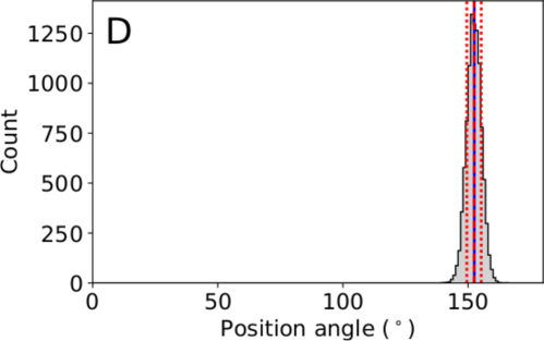
(a) Example 1 - narrow LQG

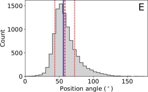
(b) Example 2 - broad LQG

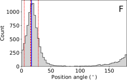
(c) Example 3 - intermediate LQG

Figure 16: LQG position angles from 10000 bootstraps for three example LQGs, labelled D, E, F in Fig. 10, and visually classified as 16(a) narrow, 16(b) broad, and 16(c) intermediate morphology. All PA calculations use the 2D approach with no parallel transport. Dashed orange line shows the circular mean of the bootstraps $\bar{\theta}$, dotted orange lines show the 68% confidence interval, solid blue line shows the observed PA.

For each LQG, to estimate the uncertainty in the mean $\bar{\theta}$, we calculate its confidence interval following Pelgrims (2016), who in turn follows Fisher (1993), and for each individual bootstrap $i$ out of a total of $n$ we define the residual as

$$\gamma_{i}=\frac{1}{2}\arctan\left(\frac{\sin(2(\theta_{i}-\bar{\theta}))}{\cos(2(\theta_{i}-\bar{\theta}))}\right)\ ,$$ (18)

where $\theta_{i}$ is the PA of the $i^{\mathrm{th}}$ bootstrap LQG. For $i=1,...,n$ we sort the $\gamma_{i}$ in ascending order to give an ordered list $\gamma_{(1)}\leq...\leq\gamma_{(n)}$. To determine the confidence interval at the $100(1-\alpha)\%$ level we find the $\gamma_{i}$ list elements at lower index $l$ which is the integer part of $(n\alpha+1)/2$ and upper index $u=n-l$. The confidence interval for $\bar{\theta}$ is then $[\bar{\theta}+\gamma_{(l+1)},\bar{\theta}+\gamma_{(u)}]$. We calculate the confidence interval at the 68% level ($\alpha=0.32$) and define the half-width of the confidence interval (HWCI) as

$$\gamma_{h}=(\gamma_{(u)}-\gamma_{(l+1)})/2\ .$$ (19)

For each of our sample of 71 LQGs, we create $n=10000$ bootstraps, calculate their PAs $\theta_{i}$ using the 2D or 3D approach (Appendix C), and then determine the mean $\bar{\theta}$ and confidence interval. Fig. 16 shows the distribution of bootstrap PAs $\theta_{i}$ calculated using the 2D approach for three example LQGs. The circular mean of the bootstraps $\bar{\theta}$ (dashed orange line) generally agrees well with the observed PA (solid blue line). As expected, the 68% confidence interval (Fig. 16, dotted orange lines) is smaller for (a) a ‘narrow’ LQG than (b) a ‘broad’ sheet-like LQG. Example (c) illustrates why the linear mean is inappropriate, since the distribution of the bootstrap PAs may ‘wrap’ from $180^{\circ}$ back to $0^{\circ}$.

The HWCIs for 10000 bootstraps of our sample of 71 LQGs, with PAs $\theta_{i}$ calculated using both the 2D and 3D approaches, are shown as error bars in Fig. 15. The mean (median) HWCI for the 2D approach is $\sim 10^{\circ}$ ($\sim 8^{\circ}$), and for the 3D approach it is $\sim 11^{\circ}$ ($\sim 9^{\circ}$).

Appendix F Applying the S test

F.1 Nearest neighbours free parameter

The S test quantifies the coherence of PA alignment by measuring the dispersion of groups of $n_{v}$ nearest neighbours, where $n_{v}$ is a free parameter. We explore a range of $n_{v}$ values; we do not choose a specific value. For each LQG, its nearest neighbours can be determined either in two dimensions (angular separation) or three dimensions (proper separation).

In 2D, nearest neighbours are identified by calculating the angular separation $\theta$ on the celestial sphere between LQG 1 and LQG 2 as

$$\theta=\cos^{-1}[\sin\delta_{1}\sin\delta_{2}+\cos\delta_{1}\cos\delta_{2}\cos(\alpha_{1}-\alpha_{2})]\ ,$$ (20)

where $\alpha_{1}$ and $\delta_{1}$ ($\alpha_{2}$ and $\delta_{2}$) are the right ascension and declination of the centroids of LQG 1 (2) respectively. For each LQG, its nearest neighbours are those $n_{v}$ LQGs separated from it by the smallest angular distances.

In 3D, nearest neighbours are identified by calculating the three-dimensional proper positions ($x$, $y$, $z$) of each LQG centroid. For each LQG, its nearest neighbours are those $n_{v}$ LQGs separated from it by the smallest proper distances.

The 2D and 3D approaches of identifying nearest neighbours will return different groups of LQGs. When these groups are used to compute the S statistic $S_{D}$ we find that the values calculated using the two approaches are remarkably consistent. This is probably due to the geometry of the three-dimensional survey volume; our redshift restriction of $1.0\leq z\leq 1.8$ yields a ‘shell’ of LQGs of finite thickness. At low $n_{v}$ the 3D approach may find neighbours in the radial direction, but at high $n_{v}$ it can only find them tangentially (on the sky), like the 2D approach. Since the two approaches give very similar results, and the 3D approach is more physically motivated, we use the 3D approach of identifying nearest neighbours in this work.

F.2 Estimating significance level

The S test yields an $S_{D}$ statistic for each number of nearest neighbours $n_{v}$ assessed. The significance level of these values compared to randomness cannot be evaluated analytically, due to: overlaps between groups of nearest neighbours, deviation of the $S_{D}$ distribution from normality (particularly for small $n$ and when $n_{v}\sim n$), and the dependence of parallel transport corrections on the precise location of the objects involved. Therefore, numerical simulations are required.

Hutsemékers (1998) and Hutsemékers & Lamy (2001) generate random samples by shuffling the observed PAs randomly between objects, while keeping their positions fixed. This has the effect of erasing any correlation between PAs and positions. But, as Jain et al. (2004) note, the shuffling method is unable to test for global alignment.

We have no reason to expect LQG PAs to be correlated with LQG positions; alignment could be global. Therefore, we generate random samples from a uniform distribution, keeping the three-dimensional LQG positions fixed. We generate $n=71$ PAs, randomly drawn from a uniform distribution. These are generated in the ranges [$0^{\circ}$, $180^{\circ}$) for 2-axial PAs and [$0^{\circ}$, $90^{\circ}$) for 4-axial PAs. Note that initially generating 4-axial PAs in the range [$0^{\circ}$, $180^{\circ}$), then converting to [$0^{\circ}$, $90^{\circ}$) after parallel transport and before evaluating the S test is equivalent.

The significance level (SL) of the S test is defined as the percentage of simulations that have an $S_{D}$ statistic at least as extreme as the one from our observations (Pelgrims, 2016). It is computed by comparing the statistic of our observations ($S_{D,obs}$) with the statistic from a large number of numerical simulations ($S_{D,sim}$).

For 2-axial PAs we find that $S_{D,obs}$ is in the low $S_{D,sim}$ (left-hand) tail of the distribution. To interpret this, consider the potential bimodality of the LQG PA distribution, with the peaks separated by $\sim 90^{\circ}$. This orthogonality leads to a large dispersion, and yields a small value of $S_{D}$. Therefore, it is legitimate to interpret a result in the left-hand tail as a potentially orthogonal signal, with the SL being the probability that $S_{D,sim}<S_{D,obs}$. This can be tested by also evaluating the S test for 4-axial PAs.

Note that two modes of a possible combined ‘alignment plus orthogonality’ signal would tend to erase any signal, reducing the power of this test. However, a residual signal in the left (right) tail indicates the orthogonality (alignment) mode dominates.

When we convert 2-axial PAs to 4-axial, we simultaneously test for alignment and orthogonality by combining the modes, so an ‘alignment plus orthogonality’ signal will manifest as alignment only. The SL is therefore the proportion of numerical simulations with statistic $S_{D}$ higher than that observed. Indeed, for 4-axial PAs we find that $S_{D,obs}$ is in the high $S_{D,sim}$ (right-hand) tail of the distribution, with the SL being the probability that $S_{D,sim}>S_{D,obs}$. Note that an ‘alignment only’ signal would also be in the right-hand tail, but would be differentiated by its 2-axial result.

The $S_{D}$ distributions of 2-axial and 4-axial numerical simulations differ, particularly as $n_{v}$ approaches $n$. Therefore, we generate separate numerical simulations for each, and calculate the significance levels as

$$\mathrm{SL_{2ax}}=P(S_{D,sim(2ax)}<S_{D,obs(2ax)})\ ,$$ (21)

$$\mathrm{SL_{4ax}}=P(S_{D,sim(4ax)}>S_{D,obs(4ax)})\ ,$$ (22)

where $P$ indicates probability, $2ax$ and $4ax$ indicate 2-axial and 4-axial PAs, and $sim$ and $obs$ indicate simulations and observations respectively.

Appendix G LQGs in 3D proper space

The 71 LQG positions in three-dimensional proper space, and their orientation as determined by the three-dimensional method, are illustrated in Fig. 17, with additional perspectives shown in Fig. 18.

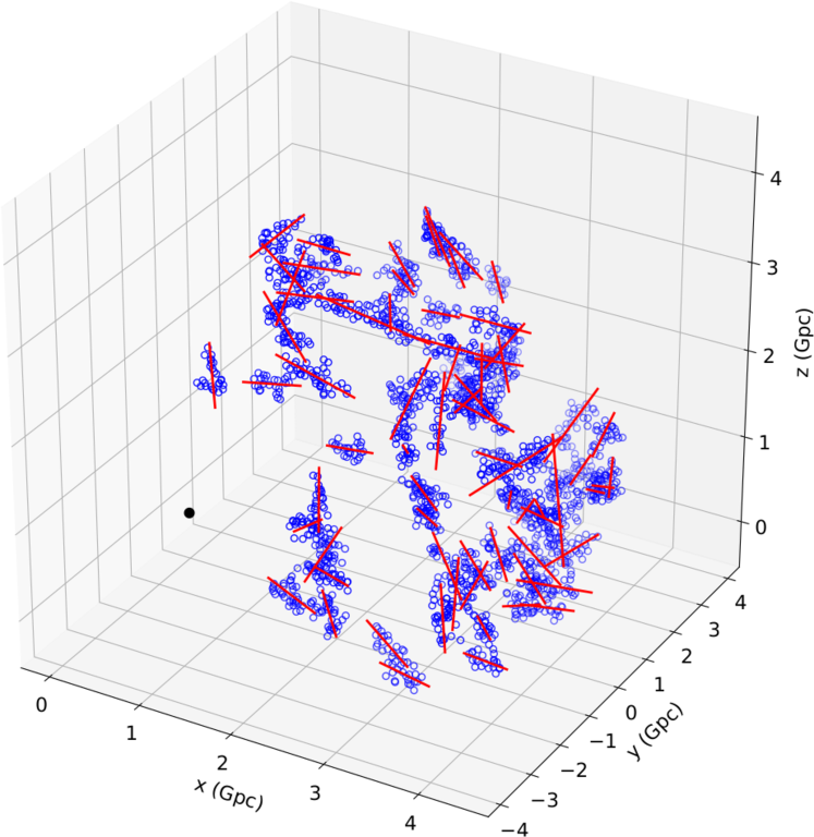
Figure 17: LQGs in three-dimensional proper space, showing LQG quasars (blue circles) and LQG major axes (red lines). Quasar markers are shaded to give the appearance of depth, with lighter shades representing more distant quasars. Our location at ($x,y,z$) coordinates (0, 0, 0) is indicated by a black dot. See Fig. 18 for three alternative, orthogonal perspectives.

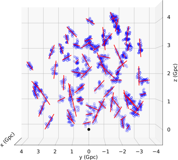
(a) $x$-axis orthogonal to the page

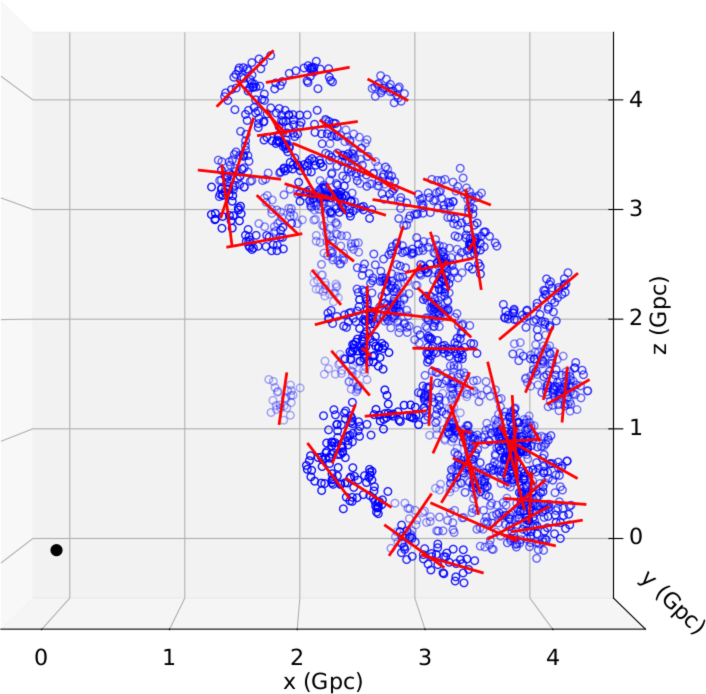
(b) $y$-axis orthogonal to the page

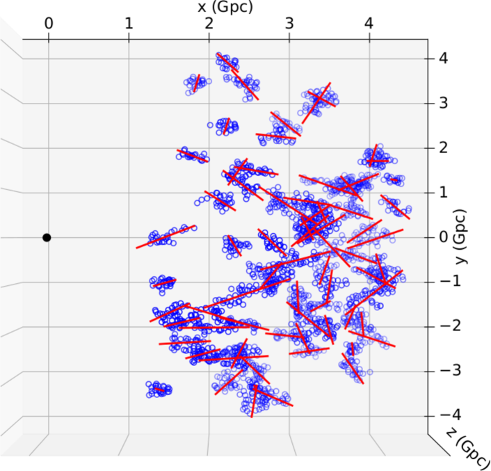
(c) $z$-axis orthogonal to the page

Figure 18: As Fig. 17 but viewed with the (a) $x$-axis, (b) $y$-axis, and (c) $z$-axis orthogonal to the page.

Appendix H Parallel transport destination

Fig. 19 shows LQG PAs after parallel transport to the location of each of the 71 LQGs. Also shown, double Gaussian fit (blue).

Figure 19: LQG position angles after parallel transport to the location of each LQG; $15^{\circ}$ bins. Solid blue lines are double Gaussian fit. The bimodal distribution is generally robust to parallel transport destination.

References

- Agarwal et al. (2011) Agarwal N., Kamal A., Jain P., 2011, Phys. Rev. D, 83, 065014
- Akaike (1974) Akaike H., 1974, IEEE Trans. Autom. Control, 19, 716
- Barrow et al. (1985) Barrow J. D., Bhavsar S. P., Sonoda D. H., 1985, MNRAS, 216, 17
- Baugh et al. (2019) Baugh C. M., et al., 2019, MNRAS, 483, 4922
- Blinov et al. (2020) Blinov D., Casadio C., Mandarakas N., Angelakis E., 2020, A&A, 635, A102
- Cabanac et al. (2005) Cabanac R. A., Hutsemékers D., Sluse D., Lamy H., 2005, in Adamson A., Aspin C., Davis C., Fujiyoshi T., eds, Astronomical Society of the Pacific Conference Series Vol. 343, Astronomical Polarimetry: Current Status and Future Directions. p. 498 (arXiv:astro-ph/0501043)
- Challinor & Chon (2002) Challinor A., Chon G., 2002, Phys. Rev. D, 66, 127301
- Clowes et al. (2012) Clowes R. G., Campusano L. E., Graham M. J., Söchting I. K., 2012, MNRAS, 419, 556
- Clowes et al. (2013) Clowes R. G., Harris K. A., Raghunathan S., Campusano L. E., Söchting I. K., Graham M. J., 2013, MNRAS, 429, 2910
- Codis et al. (2018) Codis S., Jindal A., Chisari N. E., Vibert D., Dubois Y., Pichon C., Devriendt J., 2018, MNRAS, 481, 4753
- Contigiani et al. (2017) Contigiani O., et al., 2017, MNRAS, 472, 636
- DESI Collaboration et al. (2016) DESI Collaboration et al., 2016, The DESI Experiment Part I: Science,Targeting, and Survey Design (arXiv:1611.00036)
- Das et al. (2005) Das S., Jain P., Ralston J. P., Saha R., 2005, J. Cosmology Astropart. Phys., 2005, 002
- Davé et al. (2019) Davé R., Anglés-Alcázar D., Narayanan D., Li Q., Rafieferantsoa M. H., Appleby S., 2019, MNRAS, 486, 2827
- Dubois et al. (2014) Dubois Y., et al., 2014, MNRAS, 444, 1453
- Efron (1979) Efron B., 1979, Ann. Statist., 7, 1
- Einasto et al. (1997) Einasto M., Tago E., Jaaniste J., Einasto J., Andernach H., 1997, A&AS, 123, 119
- Einasto et al. (2014) Einasto M., et al., 2014, A&A, 568, A46
- Feigelson & Babu (2012) Feigelson E. D., Babu G. J., 2012, Modern Statistical Methods for Astronomy. Cambridge University Press
- Fisher (1993) Fisher N. I., 1993, Statistical Analysis of Circular Data. Cambridge University Press
- Freeman & Dale (2013) Freeman J. B., Dale R., 2013, Behav. Res., 45, 83
- Ganeshaiah Veena et al. (2018) Ganeshaiah Veena P., Cautun M., van de Weygaert R., Tempel E., Jones B. J. T., Rieder S., Frenk C. S., 2018, MNRAS, 481, 414
- Graham et al. (1995) Graham M. J., Clowes R. G., Campusano L. E., 1995, MNRAS, 275, 790
- Hartigan & Hartigan (1985) Hartigan J. A., Hartigan P. M., 1985, Ann. Statist., 13, 70
- Hermans & Rasson (1985) Hermans M., Rasson J. P., 1985, Biometrika, 72, 698
- Hewett & Wild (2010) Hewett P. C., Wild V., 2010, MNRAS, 405, 2302
- Hutsemékers (1998) Hutsemékers D., 1998, A&A, 332, 410
- Hutsemékers & Lamy (2001) Hutsemékers D., Lamy H., 2001, A&A, 367, 381
- Hutsemékers et al. (2005) Hutsemékers D., Cabanac R., Lamy H., Sluse D., 2005, A&A, 441, 915
- Hutsemékers et al. (2010) Hutsemékers D., Borguet B., Sluse D., Cabanac R., Lamy H., 2010, A&A, 520, L7
- Hutsemékers et al. (2011) Hutsemékers D., Payez A., Cabanac R., Lamy H., Sluse D., Borguet B., Cudell J., 2011, in Bastien P., Manset N., Clemens D. P., St-Louis N., eds, Astronomical Society of the Pacific Conference Series Vol. 449, Astronomical Polarimetry 2008: Science from Small to Large Telescopes. p. 441 (arXiv:0809.3088)
- Hutsemékers et al. (2014) Hutsemékers D., Braibant L., Pelgrims V., Sluse D., 2014, A&A, 572, A18
- Icke & van de Weygaert (1987) Icke V., van de Weygaert R., 1987, A&A, 184, 16
- Isobe et al. (1990) Isobe T., Feigelson E. D., Akritas M. G., Babu G. J., 1990, ApJ, 364, 104
- Jackson (1972) Jackson J. C., 1972, MNRAS, 156, 1P
- Jaffe et al. (2005) Jaffe T. R., Banday A. J., Eriksen H. K., Górski K. M., Hansen F. K., 2005, ApJ, 629, L1
- Jain et al. (2004) Jain P., Narain G., Sarala S., 2004, MNRAS, 347, 394
- Joshi et al. (2007) Joshi S. A., Battye R. A., Browne I. W. A., Jackson N., Muxlow T. W. B., Wilkinson P. N., 2007, MNRAS, 380, 162
- Kaiser (1987) Kaiser N., 1987, MNRAS, 227, 1
- Kim et al. (2011) Kim J., Park C., Rossi G., Lee S. M., Gott J. R. III., 2011, JKAS, 44, 217
- Kraljic et al. (2020) Kraljic K., Davé R., Pichon C., 2020, MNRAS, 493, 362
- Kuiper (1960) Kuiper N. H., 1960, Indagationes Mathematicae (Proceedings), 63, 38
- Landler et al. (2018) Landler L., Ruxton G. D., Malkemper E. P., 2018, Behav. Ecol. and Sociobiol., 72, 128
- Landler et al. (2019) Landler L., Ruxton G. D., Malkemper E. P., 2019, BMC Ecology, 19, 30
- Mandarakas et al. (2021) Mandarakas N., Blinov D., Casadio C., Pelgrims V., Kiehlmann S., Pavlidou V., Tassis K., 2021, A&A, 653, A123
- Mardia & Jupp (2000) Mardia K., Jupp P., 2000, Directional statistics. Wiley series in probability and statistics, Wiley
- Marinello (2015) Marinello G. E., 2015, PhD thesis, University of Central Lancashire
- Marinello et al. (2016) Marinello G. E., Clowes R. G., Campusano L. E., Williger G. M., Söchting I. K., Graham M. J., 2016, MNRAS, 461, 2267
- Maurus & Plant (2016) Maurus S., Plant C., 2016, in Proceedings of the 22nd ACM SIGKDD International Conference on Knowledge Discovery and Data Mining. KDD ’16. Association for Computing Machinery, New York, NY, USA, p. 1055–1064, doi:10.1145/2939672.2939740, https://doi.org/10.1145/2939672.2939740
- Merloni et al. (2019) Merloni A., et al., 2019, The Messenger, 175, 42
- Monahan (2011) Monahan J. F., 2011, Numerical Methods of Statistics, 2 edn. Cambridge Series in Statistical and Probabilistic Mathematics, Cambridge University Press
- Nadathur (2013) Nadathur S., 2013, MNRAS, 434, 398
- Park et al. (2012) Park C., Choi Y.-Y., Kim J., Gott J. R. III., Kim S. S., Kim K.-S., 2012, ApJ, 759, L7
- Park et al. (2015) Park C., Song H., Einasto M., Lietzen H., Heinamaki P., 2015, JKAS, 48, 75
- Payez et al. (2008) Payez A., Cudell J. R., Hutsemékers D., 2008, in Cugon J., Lansberg J.-P., Matagne N., eds, American Institute of Physics Conference Series Vol. 1038, Hadronic Physics: Joint Meeting Heidelberg-Liège-Paris-Wroclaw - HLPW 2008. pp 211–219 (arXiv:0805.3946)
- Payez et al. (2011) Payez A., Cudell J. R., Hutsemékers D., 2011, Phys. Rev. D, 84, 085029
- Pelgrims (2016) Pelgrims V., 2016, PhD thesis, Université de Liège (arXiv:1604.05141)
- Pelgrims (2019) Pelgrims V., 2019, A&A, 622, A145
- Pelgrims & Cudell (2014) Pelgrims V., Cudell J. R., 2014, MNRAS, 442, 1239