Block-encoding dense and full-rank kernels using hierarchical matrices: applications in quantum numerical linear algebra
Abstract
Many quantum algorithms for numerical linear algebra assume black-box access to a block-encoding of the matrix of interest, which is a strong assumption when the matrix is not sparse. Kernel matrices, which arise from discretizing a kernel function , have a variety of applications in mathematics and engineering. They are generally dense and full-rank. Classically, the celebrated fast multipole method performs matrix multiplication on kernel matrices of dimension in time almost linear in by using the linear algebraic framework of hierarchical matrices. In light of this success, we propose a block-encoding scheme of the hierarchical matrix structure on a quantum computer. When applied to many physical kernel matrices, our method can improve the runtime of solving quantum linear systems of dimension to , where and are the condition number and error bound of the matrix operation. This runtime is near-optimal and, in terms of , exponentially improves over prior quantum linear systems algorithms in the case of dense and full-rank kernel matrices. We discuss possible applications of our methodology in solving integral equations and accelerating computations in N-body problems.
1 Introduction
One of the most promising applications of quantum information processing is in solving linear algebraic problem in high dimensions efficiently. Since the Harrow-Hassidim-Lloyd (HHL) algorithm was first developed for solving linear systems of equations [1], a number of improvements have been proposed. Significantly, the breakthrough algorithms in [2] and [3] solved sparse linear systems of equations in time polylogarithmic in the system size and the target error bound . When these algorithms are applied to dense matrices, however, their complexity scales linearly in (see Table 1). Using a quantum random access memory (QRAM) data structure [4], the work of [5] improved the runtime to . Classically, quantum-inspired algorithms [6, 7] use an analog of QRAM called sample-query access and apply sketching techniques [8] to solve linear systems with runtimes independent of but scaling poorly with the rank of the matrix as (see Appendix A).
In fact, achieving a runtime logarithmic in for dense and full-rank matrices is generally challenging unless there are specific symmetries or structures inherent in the matrix. For example, quantum algorithms have been developed to achieve polylogarithmic complexity in for Toepliz systems [9], Hankel matrices [10], and linear group convolutions [11] which all feature the group quantum Fourier transforms (QFT) [12] to implement operations as sparse matrices in the Fourier basis. This approach of using group QFTs, however, only applies for certain groups and requires the matrix entries to be exactly uniformly sampled from a generating function, thus inapplicable to more general settings (e.g., matrix entries corresponding to atoms on a lattice vibrating around their equilibrium positions).
Kernel matrices are a class of matrices whose entries are calculated as a function of a kernel . They have applications in mathematical physics [13], engineering [14] and machine learning [15], where they are often obtained by sampling or discretizing a smooth kernel that reflects the physical model at hand. In general, kernel matrices are dense and full-rank. Hierarchical matrices (-matrices) [16, 17] are a classical framework for efficiently performing matrix operations on commonly found kernel matrices by hierarchically splitting the “space" dimension of the matrix entries. In terms of the matrix dimension , classically performing matrix-vector multiplication with -matrices takes time which is a significant improvement over the generic time. This -matrix structure lies at the heart of the celebrated fast multipole method [13]. This improvement intuitively arises because kernel matrices often decay or change slowly along entries that are farther from the diagonals of the matrix. -matrices progressively approximate the matrix in larger low-rank blocks for farther off-diagonal entries to efficiently implement kernel matrices.
We present an efficient quantum algorithm to implement -matrices in the block-encoding framework, which embeds matrices inside a unitary operator that can be queried multiple times. This construction, which is at the core of many quantum algorithms, allows one to conveniently perform matrix computations on a quantum computer [18, 19, 20, 21]. As many recently proposed algorithms use block-encodings as a black box, one of the major challenges for quantum numerical linear algebra in this framework is to efficiently block-encode matrices so that the asymptotic runtimes are efficient even when the block-encoding complexity is included. Our -matrix block-encoding procedure, combined with existing quantum linear systems algorithms, e.g., adiabatic solver in [22], provides near-optimal runtime in solving quantum linear systems for many typical kernels that are neither sparse nor low-rank, e.g., (see Table 1 for comparisons to prior work). Apart from the -matrix block-encoding, we also provide in the Appendix a list of common kernel matrices that can be efficiently block encoded using existing techniques.
We proceed as follows. First, we overview classical hierarchical matrices in Section 2 and the quantum block-encoding framework in Section 3. We then present an algorithm for efficiently block-encoding hierarchical matrices and apply this to kernel matrices in Section 4. In Section 4.4, we generalize our methodology to construct block encodings for a more general class of matrices whose structure is derived from hierarchical matrices. Finally, we discuss applications of our algorithm in calculating -body gravitational potentials and solving integral equations in Section 5.
2 Background in -matrices and hierarchical splitting
To observe why hierarchical matrices are useful, consider a physical model which requires summation or integration over spacetime. The -body gravitational force problem [23], for example, requires evaluating potentials of the form
| (1) |
where and denote the mass and location of particle . Summing or integrating over all particles is equivalent to performing matrix-vector multiplication, generally requiring operations unless the underlying matrix is sparse or has special properties. As we will show, when particles are placed in a favorable arrangement (e.g., approximately uniformly), this matrix-vector multiplication can be approximately performed in time .
Hierarchical matrices (-matrices) [16, 17, 24] are a powerful algebraic framework for accelerating matrix computations involving displacement kernels which satisfy certain properties outlined below. The key idea is to (i) split the kernel matrix into hierarchically off-diagonal blocks and (ii) approximate each block by a low-rank matrix. This low rank approximation is justified because off-diagonal blocks represent distant interactions that are small or slowly changing with distance. We now detail the two ingredients of -matrices, namely the hierarchical splitting and the off-diagonal low-rank approximation.
2.1 Hierarchical splitting into admissible blocks
Hierarchical splitting partitions a kernel matrix into so-called “admissible” blocks where entries representing more distant interactions are grouped together into larger blocks. Consider a system of particles, whose pairwise interaction is described by the kernel . The kernel matrix of this system is defined as
| (2) |
where is the location of particle . For ease of analysis, we assume the particles are uniformly distributed and choose and . For example, this is the case when the kernel matrix is obtained by discretizing an integral operator over the domain (see [16]). In general, a kernel matrix need not be square and the source locations need not be 1-dimensional nor equally spaced and we will show how to generalize the current setup to these cases in later sections. We refer the interested readers to [25, 26, 17, 27, 28] for further details.
A set of particles located at is denoted as a cluster , storing the list of individual indices .
Definition 2.1 (Admissible blocks).
Let and . Let be a partition of , i.e., . For a cluster , define the center of as and the radius of as Furthermore, for , define the distance between the two clusters and as Then, the matrix block is called admissible if , where .
Informally, a block is admissible if the distance between its two corresponding clusters is larger than their radii (other values of can give rise to different forms of the hierarchical splitting, see [25, 16]). We now split the matrix into a hierarchy of admissible blocks consisting of levels of decreasing radii. At level , define the following partition of :
| (3) |
where
| (4) |
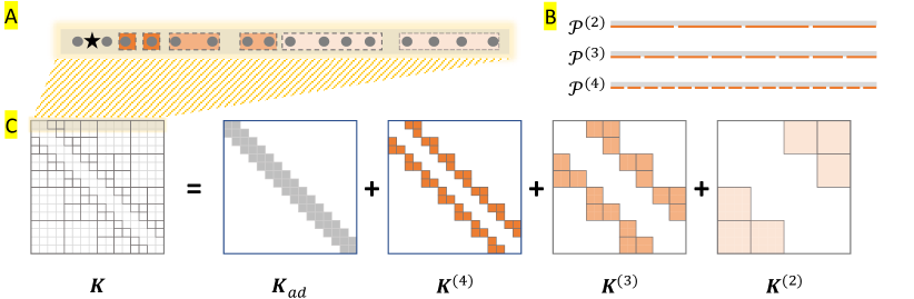
For example, , , and for are shown in Figure 1B. Note that admissible blocks only exist for . We now construct a hierarchical splitting of our kernel matrix into admissible blocks starting from the coarsest level . First, we split into admissible and inadmissible blocks in
Next, we split into admissible and inadmissible blocks in (excluding the admissible blocks of that are already covered in )
Recursively applying the decomposition up to level , we obtain a hierarchically structured representation of
| (5) |
where is a tridiagonal matrix which represents the “adjacent" interaction of neighboring particles (see Figure 1C). Observe that the matrices are block-sparse; that is, each block-row or block-column of contains at most three non-zero admissible blocks. Furthermore, these blocks represent “far-field” interactions which can be approximated by low-rank matrices if the kernel satisfies some additional properties discussed in the next section.
In Section D.3, we describe a generalization of the hierarchical splitting to higher dimensions, where the two key properties still hold, i.e., there are only levels and each level is block-sparse.
2.2 Low-rank approximation of admissible blocks
For far-field interactions in admissible blocks, the kernel can be well approximated by a truncated Taylor series if it satisfies the following asymptotic smoothness condition:
| (6) |
where is a constant. For instance, the log kernel directly satisfies the above. This condition enables approximating any admissible block by a rank- matrix
| (7) |
where , and
| (8) | |||
| (9) |
Here, regulates the precision of the approximation (typically for an error bound ). A detailed example and error analysis of this far-field approximation can be found in Appendix D. In addition, we note that conditions other than that of Equation 6 can also be used to justify the approximation (see [29, 30, 31]) of admissible blocks by low-rank kernels .
Combining this low-rank approximation and the hierarchical splitting forms a complete -matrix. In Appendix D, we show that matrix-vector multiplication with an -matrix can be performed in time . In addition, other -matrix operations such as matrix-matrix multiplication and matrix inversion run in time , we refer the reader to [25, 16, 24] for further details. The rank can be chosen at each level to further optimize computational complexity versus approximation error [26].
3 Block-encoding arithmetic
Throughout this paper, we employ the block-encoding framework to perform matrix computations on a quantum computer [18]. Here, an -qubit (non-unitary) operator (let ) is embedded in a unitary operator using ancilla qubits such that the top left block of is proportional to :
| (10) |
where is the normalization factor of the block-encoding. Formally, the -qubit unitary is an -block-encoding of if
| (11) |
where denotes the operator norm of a matrix and is the identity operator on qubits. In other words, applying the unitary to a quantum state and post-selecting on the measurement outcome on the ancilla qubits is equivalent to applying the operation on :
| (12) |
where is a garbage state that is orthogonal to the subspace , i.e., . The probability of successfully post-selecting is thus equal to . Observe that is required to embed inside a unitary matrix. Further, since the probability of success of the post-selection step depends on the ratio , a block-encoding is optimal if . More generally, if the ratio grows logarithmically with the size of the matrix , the probability of success also only changes logarithmically with . More generally, as we will see some examples in Section 5, the complexity of quantum algorithms [3] in the block-encoding framework depends on the ratio . This important observation motivates the following definition of a “good” block-encoding.
Definition 3.1 (Good block-encoding).
Given a matrix , an -block-encoding of is good if and only if the ratio , and additionally, and the circuit depth of is . The block-encoding is called optimal if .
Throughout this paper, we assume that matrices are normalized to have the largest entry at most , and we analyze the optimality of block-encodings by comparing the normalization factor to the operator norm .
Before proceeding to block-encode a hierarchical matrix, we provide various methods for block-encoding the individual matrix blocks in the hierarchical splitting. Depending on the locations of the matrix blocks and how the values of the kernel entries can be accessed by a quantum computer, there are various different ways one can block-encode a given matrix. Previous work has proposed efficient means to block-encode sparse matrices, purified density matrices, etc., as well as transformations of these matrices in the block-encoding framework [3, 32, 18]. We list some previously established results in this framework in Appendix B, among which we particularly use Lemma B.5 to block-encode sparse matrices with oracle access to entries, Lemma B.3 to linearly combine block-encoded matrices, and Lemma B.4 to multiply block-encoded matrices. Later, we will apply and combine these individual block-encoding Lemmas to form a block-encoding of the complete hierarchical matrix.
First, we provide a version of Lemma B.5 applied to dense matrices, which we refer to as the “naive” block-encoding approach since it is unaware of the inherent structure of the block-encoded matrix.
Lemma 3.2 (Naive block-encoding of dense matrices with oracle access).
Let (where ) and let . Suppose the following oracle is provided
where and is the (exact) -qubit description of . Then one can implement a -block-encoding of with two uses of , one- and two-qubit gates and extra qubits (which are discarded before the post-selection step).
Assuming , the normalization factor of this block-encoding is , which is suboptimal if , e.g., this situation arises when the matrix has many small entries. This suboptimal block-encoding could lead to an exponentially small probability of success in the post-selection step. Therefore, a structure-aware block-encoding procedure is needed to achieve an optimal runtime in terms of .
To directly implement the -matrices outlined in Section 2, we need procedures to block-encode block-sparse and low-rank matrices which we provide in the Lemmas below (all proofs are deferred to Appendix B). First we define state preparation pairs, which are frequently used in this study to prepare the coefficients in a linear combination of matrices.
Definition 3.3 (State preparation pair [3]).
Let and , the pair of unitaries is called a -state-preparation-pair of if and such that and for any .
Next, we show how to implement a block-encoding of low-rank matrices.
Lemma 3.4 (Block-encoding of low-rank operators with state preparation unitaries, inspired by Lemma 1 of [33]).
Let where . Let and . Suppose the following -qubit unitaries are provided:
where and is the quantum state whose amplitudes are the entries of . Let be a -state-preparation-pair for the vector . Then, one can construct a -block-encoding of with one use of each of , and a gate on two -qubit registers.
The above lemma provides one method to block-encode the approximately low-rank matrices described in Section 2, but as we will see, is not the only option one has at their disposal. When the rank of a matrix is small and bounded, the time needed to prepare unitaries is typically negligible; e.g., they can be efficiently implemented with an oracle providing access to (and is close to the sum of the singular values). In addition, the unitaries can be constructed using existing state preparation methods based on the structure of the entries in the singular vectors (e.g., [34] utilized efficiently integrable distributions, [4] used a QRAM data structure). In Section B.3, we also present an approach to efficiently construct from oracles providing access to the entries of for cases where the entries change slowly (Lemma B.8).
Next, the following lemma block-encodes a block-sparse matrix, whose blocks are also block-encoded.
Lemma 3.5 (Block-encoding of block-sparse matrices).
Let be a -row-block-sparse and -column-block-sparse matrix, where each is an -qubit operator. Let be an -block-encoding of . Suppose that we have the access to the following -qubit oracles
where , , is the index for the -th non-zero block of the -th block-row of A, or if there are less than non-zero blocks, then , and similarly is the index for the -th non-zero block of the -th block-column of , or if there are less than non-zero blocks, then . Additionally, suppose the following oracle is provided:
where and is the -qubit description of (if or is out of range then ), and let the -qubit unitary . Let . Then one can implement an -block-encoding of , with one use of each of and , two uses of , additional one- and two-qubit gates, and added ancilla qubits.
Remark 3.6.
Lemma 3.5 is efficient when the matrix is sparse over blocks (where each block may be dense), which is not in general the same as the matrix being sparse. It generalizes Lemma 48 of [3] (also see Lemma B.5) for block-encoding matrices with oracle access to entries. In addition, if are the same for all blocks, we do not need the oracle , hence some ancilla qubits and gates can be saved (see proof in Section B.4).
4 Block-encoding of kernel matrices via hierarchical splitting
In this section, we apply the block-encoding techniques delineated in Section 3 to block-encode -matrices. Our goal is to obtain good block-encodings (Definition 3.1) of these matrices where the ratio between the normalization factor and the operator norm is at most . We provide an optimal block-encoding procedure for kernel matrices arising from a variety of polynomially decaying and exponentially decaying kernels. We show that using only the hierarchical splitting without subsequent low-rank approximation gives an optimal block-encoding for these kernel matrices, enabling matrix transformations (e.g., multiplication, inversion, polynomial transformations) with optimal query and gate complexities. Then, we provide a block-encoding procedure for general -matrices whose admissible blocks are approximated by low-rank matrices and discuss the applicability of our procedure on other variants of hierarchical splitting.
4.1 Polynomially decaying kernels
We use the hierarchical splitting described in Section 2 to implement an optimal block-encoding procedure for polynomially decaying kernels, which take the following form
| (13) |
where and represents self-interaction terms (e.g., in Coulomb point source interactions). For concreteness, we consider the problem of computing pairwise interactions in a system of particles. Particularly, consider a 1D system of particles , where and are the location and mass of the particle , respectively. The potential at is the sum over the pairwise interactions
| (14) |
For simplicity and ease of analysis, we consider a system of equally distanced particles in which and for any , where . Note that we choose the domain to be instead of as considered in Section 2, so that the maximum entry in the kernel matrix is . Had the particles been placed in the region , we could simply downscale the matrix by dividing it by so that the entries are bounded by . Recall from Section 3 that doing so does not change the block-encoding and algorithmic runtime as these depend on the ratio between the operator norm and the normalization factor. This ratio is unchanged under global rescaling of the matrix because the normalization factor will rescale accordingly in the block-encoding procedure.
To access the kernel function on a quantum computer, we assume the following oracle is given
| (15) |
where is the -qubit description of . In fact, if the function can be computed via an efficient classical circuit, one can construct a comparably efficient quantum circuit for [35]. In particular, this is the case when the distribution of particles is known and efficiently computable (e.g. are equally spaced points in the discretization of integral operators).
We optimally block-encode the kernel matrix up to error with a normalization factor of by using only two queries to and additional resources (i.e., one- and two-qubit gates and ancilla qubits). At a high level, our method proceeds as follows. First, we decompose into a hierarchical structure of admissible blocks as described in Section 2
| (16) |
Note that this hierarchical decomposition can also be performed in higher dimensional systems (see Section D.3). Next, for each admissible block (which is a dense matrix) in the level , we block-encode it by using the naive procedure for dense matrices (Lemma 3.2). Then, we use the procedure for block-sparse matrices (Lemma 3.5) to form a block-encoding of . Finally, we sum over hierarchical levels to obtain a block-encoding of .
Specifically, at level of the hierarchy, each admissible block has dimension . In addition, the minimum pairwise distance between particles in an admissible block in is , so the maximum entry of an admissible block in is bounded by . It follows that an admissible block at level can be -block-encoded via the naive procedure for dense matrices (Lemma 3.2), where , using two queries to and additional one- and two-qubit gates. Note that in using Lemma 3.2 to block-encode a block at level , one actually needs to query rather than itself. This is readily achieved from the oracle by conditioning on a register that indexes the level and the block indices (see Section C.1 for details). From here, each , which is a block-sparse matrix of block-sparsity 3, can be -block-encoded via Lemma 3.5 (particularly Remark 3.6). Observe that while is a matrix, the normalization factor of this block-encoding is only , which is better than the normalization factor of that one would get when naively applying Lemma 3.2 to block-encode . In addition, we still only need two queries to and additional gates because all blocks are constructed in parallel in Lemma 3.5 (see detailed analysis in Section C.1).
The adjacent interaction part , which is a tridiagonal matrix, can be -block-encoded with the procedure for sparse matrices (Lemma B.5), using two queries to and one- and two-qubit gates. Finally, we use the procedure for linearly combining block-encoded matrices (Lemma B.3) to obtain a block-encoding of as . This step requires a -qubit state preparation pair (Definition 3.3) which prepares the coefficients in the linear combination. We neglect the error in implementing this state preparation pair since it can be performed with qubit operations (see Section C.1). This entire procedure results in a -block-encoding of the exact kernel matrix , where for ,
| (17) | ||||
As before, the linear combination step does not significantly increase the circuit complexity since all levels can be constructed in parallel with only two queries to the oracle . See Section C.1 for more detailed analysis of the entire block-encoding procedure.
Remark 4.1 (Optimality).
The block-encoding of the polynomially decaying kernels in Equation 13 is optimal in the normalization factor . Indeed, a lowerbound on the operator norm of can be obtained by evaluating the norm of the vector , where is the normalized all-ones state. Observe that, . Thus, for , and for , . Clearly, the existence of our block-encoding procedure also implies that these (up to a constant factor) are an upper bound for .
Remark 4.2 (Generalized polynomially decaying kernel).
Since the above analysis only relies on the maximum entry in admissible blocks, it still holds for the case of non-uniform (bounded) masses or more general kernels of the form , where is a bounded function such as , , etc. In these cases, we simply scale the kernel matrix such that the maximum entry is (if needed) and apply the above analysis. This generalized class includes a variety of kernels, ranging from power-law interactions to common Green’s functions [36].
The above block-encoding procedure similarly applies for higher-dimensional settings where coordinates are in a -dimensional space with constant. In Section D.3, we show that there are still only hierarchical levels in this higher dimensional setting and that each level is still block-sparse. The two key features of the hierarchical splitting that allow for optimal block-encodings are maintained, and the normalization factor is still . The above optimal block-encoding construction and remarks are summarized in the following lemma.
Lemma 4.3 (Optimal block-encoding of polynomially decaying kernel matrix using -matrix).
Let , where and is a bounded function, i.e. . Assume there exists an efficient quantum circuit that performs where is a qubit string description of . Then the matrix can be -block-encoded with using the hierarchical matrix splitting. That is, the block-encoding is optimal according to Definition 3.1. This block-encoding can be constructed with two queries to and additional one- and two-qubit gates.
Our block-encoding procedure is optimal for common kernel matrices, which are neither sparse nor low-rank, thus expanding the scope of application of quantum computers in the block-encoding framework. In Section 5, for example, we discuss applications of this block-encoding in -body force computations and solving quantum linear systems.
Remark 4.4.
When sources are not close to uniformly distributed, one must first apply classical adaptive methods [27, 28] which discretize the domain to form a finer mesh, such that the number of nonzero-mass sources in each mesh site is . The dimension of the kernel matrix in this method depends on the inverse of the smallest pairwise distances between the actual sources. Therefore, the runtime of the block-encoding remains polylogarithmic in the number of particles so long as the minimum pairwise distance is not exponentially small (see Section C.3).
4.2 Exponentially decaying kernels
The procedure used in the previous section readily generalizes to exponentially decaying kernels. Consider, for example, the following kernel
| (18) |
where and is a function growing polynomially or slower. Specifically, . Typical kernels of this form include the Laplace and Gaussian kernels, which are commonly used in machine learning [15].
As before, we first hierarchically decompose the matrix into admissible blocks. For each admissible block at level , the minimum pairwise distance between particles is and therefore the maximum entry in the block can be bounded as
| (19) | ||||
where we choose an integer that satisfies .
Thus, an admissible block at level can be -block-encoded via the naive procedure for dense matrices (Lemma 3.2), where . From here, an efficient block-encoding of can be obtained via the same procedure described in the previous section, where is now replaced by . It can be verified that the normalization factor of this block-encoding is , which is optimal since the maximum entry of is of magnitude .
We note, however, that one can make use of a sparsification approach, in which the is approximated as a sparse band matrix, and apply the block-encoding procedure for a sparse matrix (Lemma B.5). This approach yields a block-encoding with normalization factor logarithmic in the sparsification error (see Section 5.3).
4.3 Block-encoding of general -matrices
In the setting most consistent with that of classical -matrix literature, one may be provided oracle access to the low-rank vectors in and which approximate an admissible block (as seen in Equation 7). Such a situation may also arise when one wants to apply an arbitrary -matrix which has no connection to any kernel function, e.g., see [37]. In this case, we can use the block-encoding procedure for low-rank matrices (Lemma 3.4) to block-encode .
After block-encoding the admissible blocks in each level of the hierarchical splitting, we follow the same procedure in previous sections to obtain the entire kernel matrix. Namely we apply the procedure for block-sparse matrices (Lemma 3.5) to construct a block-encoding of for each level of the hierarchy; then we sum over all levels using the procedure for linear combination of block-encoded matrices (Lemma B.3) to obtain a block-encoding of . The normalization factor of the block-encoding of is bounded as
| (20) |
where is normalization factor of the admissible blocks at level (for ease of analysis we assume admissible blocks at the same level have the same block-encoding normalization factor). As before, assuming the maximum entry of is 1, the naive block-encoding (Lemma 3.2) yields a block-encoding with a normalization factor of , the dimension of the matrix. Whereas, -matrix block-encoding can yield an exponentially better normalization factor over the naive approach when are . This is not the case for some kernels studied in classical -matrix literature [25, 13] such as the log kernel and the multiquadric kernel . In fact, we show in Section C.6 that these particular kernels and most polynomially growing kernels can already be optimally block-encoded using the naive approach of Lemma 3.2. The naive approach works intuitively because these kernels are numerically low-rank and their top singular vectors are nearly uniform.
4.4 Variants of hierarchical splitting
The form of the hierarchical splitting can be slightly modified for other types of decaying kernels. For example, consider kernels of the form on the domain and is an integer. In this case, we can use a “shifted” hierarchical splitting to obtain an optimal block-encoding of the kernel matrix , in which the hierarchy is shifted in the horizontal direction (along the rows). Similarly, for kernels of the form (), we can apply a shifted hierarchical splitting along the skew-diagonal direction. We illustrate this approach in Section C.2.
In Section C.4, we also describe a more general block-encoding that exploits the structure of entry magnitudes in a given matrix even if the entries of the admissible blocks are not neighboring (in fact, Definition 2.1 does not require the entries of an admissible block to be contiguous). At a high level, we use a pointer oracle which, conditioned on the level , points to the entries whose magnitudes are in the range . When this oracle can be efficiently implemented, this block-encoding procedure might find applications in other classes of dense matrices.
Proposition 4.5 (Block-encoding using generalized hierarchical splitting).
Let be a Hermitian matrix with non-negative entries which are provided via an oracle , where is an exact bit string description of . Suppose and . For any and a column , define its level- row-index subset to be and let . Suppose there exist and such that for any . Furthermore, suppose there exists an invertible function which returns the row index of the -th element (according to some fixed ordering, e.g. from top to bottom in the column) in . Then, one can construct a block-encoding of with a normalization factor of at most using two queries to , elementary gates, and ancilla qubits.
Intuitively, measures how balanced the magnitudes of the matrix entries are across rows and columns. If , this yields a good block-encoding according to Definition 3.1. For instance, is a constant for kernel matrices. In the proof of 4.5, we also present an efficient state preparation procedure using methods of -matrix splitting in Section C.4, which could be of independent interest.
5 Applications
In this section, we discuss applications of our quantum hierarchical block-encoding method in two commonly studied settings: (i) gravitational potential calculation [23] and (ii) solving integral equations [13]. The first problem requires performing matrix-vector multiplication on a quantum computer, while the second problem is equivalent to solving a quantum linear system. We also compare our procedure to the sparsification approach and address potential issues with large condition numbers.
We first state the following lemmas, which allow one to apply a block-encoded matrix or its inverse to a quantum state. Other polynomial transformations of block-encoded matrices can be performed by the quantum singular value transform (Theorem 17 of [3]).
Lemma 5.1 (Applying block-encoded matrices).
If is an -block-encoding of the matrix and is a unitary that prepares the -qubit quantum state , then it takes queries to and to obtain a quantum state such that , where is the condition number of .
Proof.
Applying the operator on the state we obtain
| (21) |
where is orthogonal to the subspace . By post-selecting the subspace , we obtain the desired quantum state . This step succeeds with a probability of . Using amplitude amplification [38], this can be improved to , giving us the specified query complexity. ∎
Lemma 5.2 (Applying inverse block-encoded matrices, adapted from [22]).
If is an -block-encoding of an invertible matrix and is a unitary that prepares the -qubit quantum state , then it takes queries to and to obtain a quantum state such that .
Proof.
We apply the main theorem of [22], which assumed to achieve a query complexity of . In general, needs to be replaced by the inverse of the minimum singular value of the block-encoded part. In our case, this singular value is . ∎
As noted in Section 3, the query complexities of the above procedures, and more generally quantum algorithms in the block-encoding framework [3], only depend on the ratio . Hence, a block-encoding is optimal (Definition 3.1) when . In the following, we apply such optimal block-encodings in Section 4 to two specific applications of kernel matrices.
5.1 Gravitational potential calculation: Quantum fast multipole method
We apply the block-encoding obtained in Section 4.1 to solve the gravitational potential problem [23] on a quantum computer. Since we use a quantum version of the hierarchical splitting, this is a quantum analogue to the classical fast multipole method [39]. Consider a 1D system of particles which are approximately uniformly distributed in the domain , where the mass and location of particle are and , respectively. Furthermore, assume that are and the smallest pairwise distance between the particles is . We would like to compute the accumulated potential at every particle , stored in a vector with entries .
Proposition 5.3 (Quantum fast multipole method).
Given an oracle that performs where is a -qubit string description of , and a procedure that prepares the quantum state which stores the normalized masses of the particles, we can obtain a quantum state that -approximates the normalized vector , whose -th entry is the accumulated potential at particle , using queries to , one- and two-qubit gates, and additional qubits.
Proof.
We first use to create the state (assume is an integer). Let , observe that . Using Lemma 4.3, we can construct a unitary , which is an -block-encoding of , with the specified gate complexity and wherein and . Then, we apply Lemma 5.1, with a more careful analysis on the post-selection step. Here, the probability of succesfully post-selecting the subspace is since and (by noting that the particle masses are and using similar calculations to those in Remark 4.1). This gives us the specified query complexity. ∎
We remark that the (non-unitary) state preparation procedure can be efficiently implemented when (see Theorem 1 of [40]). In addition, if particles are not (nearly) uniformly distributed, we can discretize the domain to form a finer mesh as described in Remark 4.4. Here we have assumed these distances are , hence the size of the mesh (and the size of the kernel matrix) is . This method also enables computing the potential at locations other than the sources themselves. This proposition also applies to -body calculations in higher-dimensional systems as the hierarchical splitting and Lemma 4.3 can be generalized to these cases (see Section D.3).
5.2 Integral equation: Quantum algorithm for linear systems of kernel matrix
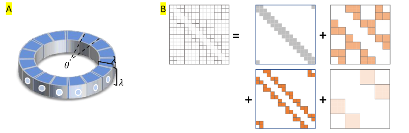
We provide an application of our hierarchical block-encoding procedure in solving a quantum linear systems of kernel matrices. These problems arise in many research areas, such as Gaussian processes [15] and integral equations [14]. Consider the following integral equation over the circular strip of unit radius and height and width as shown in Figure 2.
| (22) |
where with , is a known smooth function, and is the unknown function we would like to solve. Equations of this form are commonly found in, e.g.,, Dirichlet problems [14], where is the Coulomb potential, is the given potential on the strip, and is the unknown charge density. Here, we use the collocation method to numerically solve this integral equation which represents the unknown function in a basis and solves for the coefficients such that the integral equation is satisfied at specified locations. Particularly, we use the piecewise-constant function as the basis if and 0 otherwise. We refer to the segment as panel . Then, the integral on the RHS of Equation 22 can be rewritten as
| (23) |
In the collocation method, we solve for the integral equation at the centroids of the panels located at . In other words, we solve the following linear system
| (24) |
where bold text indicates discretized values, e.g.,, and .
Observe that this collocation method can handle the singularity when as . Furthermore, when is large, . For panels , close to each other (e.g., ), simple adaptive methods can be used to approximate the integral. For instance, one can subdivide the panel into eight smaller panels and approximate the integral as the sum of these eight sub-panels; we neglect the details and refer the interested reader to [41]. In summary, the entries of are simple to calculate and they approximately are
| (25) |
The error bound and the uniqueness of the solution in the collocation method are well-studied in classical literature, we refer to [14, 41, 42] for more details.
We now proceed to block-encode this kernel matrix. Observe that for any panels such that , hence we can apply a “cyclic” version of the hierarchical splitting in Section 2 to optimally block-encode (see Figure 2B). As analyzed in Section 4.1, this block-encoding only has a circuit depth of and a normalization factor of , as the operator norm can be lowerbounded using the same technique as in Remark 4.1 by noticing that for any .
Finally, it is straightforward to use Lemma B.3 (linear combination of block-encoded matrices) to obtain an optimal block-encoding of . Then, we directly apply Lemma 5.2 to solve the linear system in Equation 24. Since the block-encoding is optimal, the query complexity is , for a total runtime of when including the circuit complexity of the block-encoding (Lemma 4.3).
Proposition 5.4 (Solving discretized integral equations).
Consider the integral equation on a ring as described in Equation 22. We first cast the equation into the linear system in Equation 24 using the collocation method with discretized points. Then, we can obtain its numerical solution as a quantum state in time , where is the condition number of the matrix in Equation 24 and is the error bound of the quantum operation.
We address two practical aspects when applying 5.4. First, we must prepare as a quantum state. In Appendix E, we present an efficient procedure for preparing in the case where is sampled from a smooth function. At a high level, our procedure prepares the quantum state in the Fourier regime, which is approximately sparse due to the smoothness of ; then we apply the quantum Fourier transform to obtain the desired real-regime state. To prove 4.5, we also present another state preparation procedure using ideas from -matrix splitting in Section C.4 which could be of independent interest. Second, the query complexity of the block-encoding depends on the condition number of the matrix , which can be bounded as follows
| (26) |
Note that here, scales with . Since we require for the collocation method to work, the operator norm , and thus , is bounded. Therefore, the runtime of 5.4 is .
5.3 Notes on sparsification approach
Since the entries of kernel matrices often decay along a row or column, one may assume that they can be approximated by only considering a sparse set of matrix entries and applying the naive block-encoding method for sparse matrices (Lemma B.5). Here, we analyze this approach showing that it is only favorable when kernel entries decay exponentially and not polynomially. In fact, the runtime of this method is exponentially worse in the target error bound compared to that of our approach. Consider the polynomially decaying kernel in Equation 13. One could attempt to approximate this kernel matrix by a band matrix of sparsity . Defining the error to be , it can be seen that the error is of magnitude . Since this integral diverges when , one can only sparsify the matrix when . In this case, to achieve an error bound of , the sparsity needs to be . Then, one can apply Lemma B.5 (block-encoding of sparse matrices) to directly block-encode the sparsified matrix with a normalization factor of using extra gates and oracle queries. This results in an exponentially worse runtime in terms of the error bound compared to our method, which has a normalization factor of .
For the exponential kernels, however, the sparsification method requires keeping or more entries per row or column. With Lemma B.5, the sparsified block-encoding has a normalization factor of using the same gate and query complexities as above. Thus, exponential kernels may admit a sparsification approach with an extra factor of in the runtime.
5.4 Notes on condition number
The condition number and its relation to the dimension of the matrix play a central role in the runtime of our algorithms. Numerical experiments shown in Section C.5 indicate that for purely polynomially decaying kernels without any regularization and ignoring self-interacting terms (diagonal entries set to zero), the condition number grows polynomially with , i.e., the minimum singular value decays with . In practice, however, the input vector often lives in the well-conditioned subspace where these smaller singular values can be ignored as observed in the gravitation example earlier. For force calculation problems, this is the case when particles have comparable masses/charges. For numerical integration or integral equations, this is equivalently the case when the input functions change slowly.
We note that Lemma 5.2 for matrix inversion uses the discrete adiabatic theorem, whose runtime depends directly on the condition number of the matrix operation. Hence, in the case where the matrix operation is ill-conditioned but the input vector lives in the well-conditioned subspace, we can use techniques that allow for filtering out small eigenvalues before the inversion step such as the QSVT [3]. The query complexity of the block-encoding in matrix inversion in this case is , where is a chosen threshold bounding the singular values in the well-conditioned subspace.
Fortunately, for applications in numerical analysis or machine learning, the kernel matrix is often regularized by an added matrix, e.g., the addition of an identity matrix as in Fredholm integral equations of the second kind or the noise matrices in Gaussian processes and kernel ridge regression [14, 15]. In the integral equation setting, this regularization is equivalent to scaling the magnitude of self-interacting terms (diagonal entries). Furthermore, if the input vector is potentially in the ill-conditioned subspace, preconditioning methods in [43] may be used to improve the condition number.
6 Conclusion
Our results show that factoring certain kernel matrices into hierarchical or -matrices leads to efficient algorithms for implementing such kernel matrices on a quantum computer, thus expanding the scope of application of quantum computers to a class of matrices which are neither low-rank nor sparse. In fact, our approach to implementing such hierarchical matrices, in a sense, blends prior quantum methods for implementing unitary block encodings by hierarchically splitting a matrix into a sparse matrix component close to the diagonal and progressively larger blocks farther away from the diagonals. Looking forward, it is an interesting question whether any extensions to the -matrix framework can lead to further improvements in the quantum setting. Classically, the most significant extension of the -matrix framework is perhaps the development of -matrices, which incorporates a further level of hierarchical nested bases to provide a logarithmic speedup in the matrix dimension for performing matrix operations [24, 44]. Furthermore, recent classical work has parameterized -matrices to integrate them into neural networks and design learning algorithms with inductive biases that match the form of the hierarchical splitting [37, 45]. Future work can study whether such parameterizations can be performed as well in the quantum setting via variational quantum algorithms or other quantum analogues to classical neural networks [46].
Acknowledgements
We thank the anonymous reviewers for helpful feedback and corrections on this paper. This project was funded by AFOSR, ARO, and DARPA. BTK acknowledges funding from the MIT Energy Initiative fellowship.
References
- [1] Aram W. Harrow, Avinatan Hassidim and Seth Lloyd “Quantum Algorithm for Linear Systems of Equations” In Physical Review Letters 103.15 American Physical Society (APS), 2009 DOI: https://doi.org/10.1103/PhysRevLett.103.150502
- [2] Andrew M. Childs, Robin Kothari and Rolando D. Somma “Quantum Algorithm for Systems of Linear Equations with Exponentially Improved Dependence on Precision” In SIAM Journal on Computing 46.6 Society for Industrial & Applied Mathematics (SIAM), 2017, pp. 1920–1950 DOI: https://doi.org/10.1137/16M1087072
- [3] András Gilyén, Yuan Su, Guang Hao Low and Nathan Wiebe “Quantum singular value transformation and beyond: exponential improvements for quantum matrix arithmetics” In Proceedings of the 51st Annual ACM SIGACT Symposium on Theory of Computing, 2019, pp. 193–204 DOI: https://doi.org/10.48550/arXiv.1806.01838
- [4] Iordanis Kerenidis and Anupam Prakash “Quantum Recommendation Systems”, 2016 DOI: https://doi.org/10.48550/arXiv.1603.08675
- [5] Leonard Wossnig, Zhikuan Zhao and Anupam Prakash “Quantum Linear System Algorithm for Dense Matrices” In Physical Review Letters 120.5 American Physical Society (APS), 2018 DOI: http://dx.doi.org/10.1103/PhysRevLett.120.050502
- [6] András Gilyén, Zhao Song and Ewin Tang “An improved quantum-inspired algorithm for linear regression” In Quantum 6 Verein zur Förderung des Open Access Publizierens in den Quantenwissenschaften, 2022, pp. 754 DOI: https://doi.org/10.22331/q-2022-06-30-754
- [7] Changpeng Shao and Ashley Montanaro “Faster quantum-inspired algorithms for solving linear systems”, 2021 DOI: https://doi.org/10.48550/arXiv.2103.10309
- [8] David P. Woodruff “Sketching as a tool for numerical linear algebra” In Foundations and Trends in Theoretical Computer Science 10.1–2 Now Publishers, 2014, pp. 1–157 DOI: 10.1561/0400000060
- [9] Lin-Chun Wan et al. “Asymptotic quantum algorithm for the Toeplitz systems” In Physical Review A 97.6 American Physical Society (APS), 2018 DOI: 10.1103/physreva.97.062322
- [10] A Mahasinghe and J B Wang “Efficient quantum circuits for Toeplitz and Hankel matrices” In Journal of Physics A: Mathematical and Theoretical 49.27 IOP Publishing, 2016, pp. 275301 DOI: 10.1088/1751-8113/49/27/275301
- [11] Grecia Castelazo et al. “Quantum algorithms for group convolution, cross-correlation, and equivariant transformations” In Physical Review A 106.3 APS, 2022, pp. 032402 DOI: 10.1103/PhysRevA.106.032402
- [12] Andrew M. Childs and Wim Dam “Quantum algorithms for algebraic problems” In Reviews of Modern Physics 82.1 American Physical Society (APS), 2010, pp. 1–52 DOI: 10.1103/revmodphys.82.1
- [13] R Beatson and Leslie Greengard “A short course on fast multipole methods” In Wavelets, multilevel methods, and elliptic PDEs, Numerical Mathematics and Scientific Computation Oxford University Press, 1997, pp. 1–37 URL: https://nyuscholars.nyu.edu/en/publications/a-short-course-on-fast-multipole-methods
- [14] Kendall Atkinson and Weimin Han “Numerical solution of fredholm integral equations of the second kind” In Theoretical Numerical Analysis Springer, 2009, pp. 473–549 DOI: https://doi.org/10.1007/978-1-4419-0458-4_12
- [15] Carl Edward Rasmussen “Gaussian processes in machine learning” In Summer school on machine learning, 2003, pp. 63–71 Springer DOI: https://doi.org/10.1007/978-3-540-28650-9_4
- [16] W. Hackbusch “A Sparse Matrix Arithmetic Based on -Matrices. Part I: Introduction to -Matrices” In Computing 62.2, 1999, pp. 89–108 DOI: 10.1007/s006070050015
- [17] W. Hackbusch and B. N. Khoromskij “A Sparse -Matrix Arithmetic. Part II: Application to Multi-Dimensional Problems” In Computing 64.1, 2000, pp. 21–47 DOI: 10.1007/PL00021408
- [18] Guang Hao Low and Isaac L. Chuang “Hamiltonian Simulation by Qubitization” In Quantum 3 Verein zur Forderung des Open Access Publizierens in den Quantenwissenschaften, 2019, pp. 163 DOI: 10.22331/q-2019-07-12-163
- [19] Shantanav Chakraborty, András Gilyén and Stacey Jeffery “The power of block-encoded matrix powers: improved regression techniques via faster Hamiltonian simulation” In ICALP, 2019 DOI: https://doi.org/10.4230/LIPIcs.ICALP.2019.33
- [20] Guang Hao Low and Isaac L. Chuang “Optimal Hamiltonian Simulation by Quantum Signal Processing” In Physical Review Letters 118.1 American Physical Society (APS), 2017 DOI: 10.1103/physrevlett.118.010501
- [21] Joran Apeldoorn and András Gilyén “Improvements in Quantum SDP-Solving with Applications” In ICALP, 2019 DOI: https://doi.org/10.4230/LIPIcs.ICALP.2019.99
- [22] Pedro CS Costa et al. “Optimal Scaling Quantum Linear-Systems Solver via Discrete Adiabatic Theorem” In PRX Quantum 3.4 APS, 2022, pp. 040303 DOI: 10.1103/PRXQuantum.3.040303
- [23] Josh Barnes and Piet Hut “A hierarchical O(N log N) force-calculation algorithm” In Nature 324.6096, 1986, pp. 446–449 DOI: 10.1038/324446a0
- [24] Steffen Börm, Lars Grasedyck and Wolfgang Hackbusch “Introduction to hierarchical matrices with applications” In Engineering Analysis with Boundary Elements 27.5, 2003, pp. 405–422 DOI: https://doi.org/10.1016/S0955-7997(02)00152-2
- [25] Markus Fenn and Gabriele Steidl “FMM and H-matrices: A Short Introduction to the Basic Idea”, 2002 URL: https://madoc.bib.uni-mannheim.de/744/1/TR-02-008.pdf
- [26] W. Hackbusch, B. Khoromskij and S. A. Sauter “On -matrices” In Lectures on Applied Mathematics Berlin, Heidelberg: Springer Berlin Heidelberg, 2000, pp. 9–29 DOI: https://doi.org/10.1007/978-3-642-59709-1_2
- [27] J. Carrier, L. Greengard and V. Rokhlin “A Fast Adaptive Multipole Algorithm for Particle Simulations” In SIAM J. Sci. Stat. Comput. 9.4 USA: Society for IndustrialApplied Mathematics, 1988, pp. 669–686 DOI: 10.1137/0909044
- [28] Jaswinder Pal Singh, Chris Holt, John L Hennessy and Anoop Gupta “A parallel adaptive fast multipole method” In Proceedings of the 1993 ACM/IEEE Conference on Supercomputing, 1993, pp. 54–65 DOI: 10.1145/169627.169651
- [29] E. Tyrtyshnikov “Mosaic-Skeleton approximations” In Calcolo 33, 1996, pp. 47–57 DOI: 10.1007/BF02575706
- [30] Achi Brandt “Multilevel computations of integral transforms and particle interactions with oscillatory kernels” In Computer Physics Communications 65.1, 1991, pp. 24–38 DOI: https://doi.org/10.1016/0010-4655(91)90151-A
- [31] Gregory Beylkin, Ronald R. Coifman and Vladimir Rokhlin “Fast wavelet transforms and numerical algorithms I” In Communications on Pure and Applied Mathematics 44, 1991, pp. 141–183 DOI: https://doi.org/10.1002/cpa.3160440202
- [32] Robin Kothari “Efficient algorithms in quantum query complexity”, 2014 URL: https://uwspace.uwaterloo.ca/handle/10012/8625
- [33] Yihui Quek and Patrick Rebentrost “Fast algorithm for quantum polar decomposition, pretty-good measurements, and the Procrustes problem”, 2021 DOI: 10.48550/arXiv.2106.07634
- [34] Lov Grover and Terry Rudolph “Creating superpositions that correspond to efficiently integrable probability distributions”, 2002 DOI: 10.48550/arXiv.quant-ph/0208112
- [35] Michael A. Nielsen and Isaac Chuang “Quantum Computation and Quantum Information” Cambridge University Press, 2011 DOI: 10.1017/CBO9780511976667
- [36] George B. Arfken, Hans J. Weber and Frank E. Harris “Chapter 10 - Green’s Functions” In Mathematical Methods for Physicists (Seventh Edition) Boston: Academic Press, 2013, pp. 447–467 DOI: https://doi.org/10.1016/B978-0-12-384654-9.00010-4
- [37] Yuwei Fan, Lin Lin, Lexing Ying and Leonardo Zepeda-Nún͂ez “A Multiscale Neural Network Based on Hierarchical Matrices” In Multiscale Modeling & Simulation 17.4, 2019, pp. 1189–1213 DOI: 10.1137/18M1203602
- [38] Gilles Brassard, Peter Høyer, Michele Mosca and Alain Tapp “Quantum amplitude amplification and estimation” In Quantum Computation and Information American Mathematical Society, 2002, pp. 53–74 DOI: 10.1090/conm/305/05215
- [39] L. Greengard and V. Rokhlin “A fast algorithm for particle simulations” In Journal of Computational Physics 73.2, 1987, pp. 325–348 DOI: 10.1016/0021-9991(87)90140-9
- [40] Kosuke Mitarai, Masahiro Kitagawa and Keisuke Fujii “Quantum analog-digital conversion” In Physical Review A 99.1 APS, 2019, pp. 012301 DOI: 10.1103/PhysRevA.99.012301
- [41] P. K. Kythe “An introduction to boundary element methods (1st ed.)” CRC Press, 1995 URL: https://www.routledge.com/An-Introduction-to-Boundary-Element-Methods/Kythe/p/book/9780367449148
- [42] W. Hackbusch “The Panel Clustering Method for BEM” In Discretization Methods in Structural Mechanics Berlin, Heidelberg: Springer Berlin Heidelberg, 1990, pp. 299–306 DOI: 10.1007/978-3-642-49373-7_28
- [43] Yu Tong, Dong An, Nathan Wiebe and Lin Lin “Fast inversion, preconditioned quantum linear system solvers, fast Green’s-function computation, and fast evaluation of matrix functions” In Physical Review A 104.3 American Physical Society (APS), 2021 DOI: 10.1103/physreva.104.032422
- [44] Lin Lin, Jianfeng Lu and Lexing Ying “Fast construction of hierarchical matrix representation from matrix–vector multiplication” In Journal of Computational Physics 230.10 Elsevier, 2011, pp. 4071–4087 DOI: 10.1016/j.jcp.2011.02.033
- [45] Yuwei Fan et al. “A multiscale neural network based on hierarchical nested bases” In Research in the Mathematical Sciences 6.2 Springer, 2019, pp. 1–28 DOI: 10.1007/s40687-019-0183-3
- [46] Marco Cerezo et al. “Variational quantum algorithms” In Nature Reviews Physics 3.9 Nature Publishing Group, 2021, pp. 625–644 DOI: 10.1038/s42254-021-00348-9
- [47] Dominic W. Berry, Graeme Ahokas, Richard Cleve and Barry C. Sanders “Efficient Quantum Algorithms for Simulating Sparse Hamiltonians” In Communications in Mathematical Physics 270.2, 2007, pp. 359–371 DOI: 10.1007/s00220-006-0150-x
- [48] Andris Ambainis “Variable time amplitude amplification and a faster quantum algorithm for solving systems of linear equations”, 2010 DOI: 10.48550/arXiv.1010.4458
- [49] Yiğit Subaşı, Rolando D. Somma and Davide Orsucci “Quantum Algorithms for Systems of Linear Equations Inspired by Adiabatic Quantum Computing” In Phys. Rev. Lett. 122 American Physical Society, 2019, pp. 060504 DOI: 10.1103/PhysRevLett.122.060504
- [50] Dong An and Lin Lin “Quantum Linear System Solver Based on Time-optimal Adiabatic Quantum Computing and Quantum Approximate Optimization Algorithm” In ACM Transactions on Quantum Computing 3.2 Association for Computing Machinery (ACM), 2022, pp. 1–28 DOI: 10.1145/3498331
- [51] Lin Lin and Yu Tong “Optimal polynomial based quantum eigenstate filtering with application to solving quantum linear systems” In Quantum 4 Verein zur Forderung des Open Access Publizierens in den Quantenwissenschaften, 2020, pp. 361 DOI: 10.22331/q-2020-11-11-361
- [52] Jonathan M. Borwein and Peter B. Borwein “Pi and the AGM: A Study in the Analytic Number Theory and Computational Complexity” USA: Wiley-Interscience, 1987 URL: https://www.wiley.com/en-us/Pi+and+the+AGM%3A+A+Study+in+Analytic+Number+Theory+and+Computational+Complexity-p-9780471315155
- [53] Sanjeev Arora and Boaz Barak “Computational Complexity: A Modern Approach” USA: Cambridge University Press, 2009 URL: https://doi.org/10.1017/CBO9780511804090
- [54] Steffen Börm, Lars Grasedyck and Wolfgang Hackbusch “Lecture notes on Hierarchical Matrices”, 2003 URL: https://www.mis.mpg.de/publications/other-series/ln/lecturenote-2103.html
- [55] Wajih Halim Boukaram, George Turkiyyah and David E. Keyes “Hierarchical Matrix Operations on GPUs: Matrix-Vector Multiplication and Compression”, 2019 DOI: https://doi.org/10.48550/arXiv.1902.01829
Appendix A Prior works on block-encoding and quantum linear systems algorithms
In this section, we provide a brief overview and discuss the runtimes of previous works in Table 1. As a reminder, the quantum linear system problem (QLSP) seeks an approximate solution to
| (27) |
such that
| (28) |
Let be the dimension; be the sparsity; be the condition number; and be the rank of the matrix , which is assumed to be square, normalized (), and Hermitian 111If not, one can consider the equivalent linear system , whose solution is .. The original HHL algorithm [1] runs in time by performing a Hamiltonian simulation of (i.e. ) and quantum phase estimation (QPE) subroutines. Here, the Hamiltonian simulation [47] and QPE steps together contribute a factor of , while the post-selection step contributes the remaining factor of .
Later, [2] noticed that the QPE step can be circumvented by utilizing the fact that the inverse function can be written, to the desired precision , as a linear combination of Chebyshev polynomials. Combining this expansion with the variable-time amplitude amplification technique in [48], they achieved a runtime of . This polynomial expansion approach is generalized in the block-encoding framework by [3, 19] to perform almost any polynomial matrix transformation with the same complexity. All these works use a naive block-encoding in the oracle-access model (Lemma 48 in [3], same as Lemma B.5 or Lemma 3.2).
In another approach, [5] used a QRAM data structure to implement a unitary whose eigenvalues are related to the singular values of (this algorithm does not require to be square or Hermitian) via its Frobenius norm . Thus, performing QPE on yields a quantum singular value estimation algorithm for . Matrix multiplication and inversion can then be implemented immediately with a rotation operator controlled on the register storing the singular values, just like done in HHL. The runtime of both operations, including the post-selection step, is For a full-rank matrix whose singular values are , we have . This QRAM model, however, is strictly stronger than the oracle-access model as it requires the entries be loaded and pre-processed in the data structure.
Recent adiabatic algorithms for QLSP [49, 50, 51] also enjoy success and culminate in [22], which achieved an optimal query complexity of by constructing a sophisticated schedule function for the adiabatic evolution. This query complexity is better than the algorithms in [2, 3, 5] and has been shown to be optimal [22]. However, all of these assume that the matrix is perfectly block-encoded inside a unitary which is generally hard to construct without prior knowledge of the structure of . The exact query complexity and total runtime in the general case is stated in Lemma 5.2 and governed by the ratio , where is the normalization factor in the block-encoding.
The runtimes shown in Table 1 are obtained by combining the optimal adiabatic solver in [22] (see Lemma 5.2) with the corresponding block-encoding used in [2, 3, 19, 4, 5]. In particular, the naive oracle-access block-encoding in [2, 3, 19] yields a normalization factor of for dense matrices. The QRAM-based block-encoding in [4, 5] yields for full-rank matrices. The runtime for matrix multiplication is simply obtained by computing the probability of success in the post-selection step after applying the block-encoding, as described in Section 3 and Lemma 5.1.
Quantum-inspired algorithms are a class of classical algorithms equipped with sample-query access, a classical analogue to QRAM. The currently fastest quantum-inspired algorithms for QLSP [6, 7] are based on stochastic gradient descent (specifically randomized Kaczmarz method) for a runtime of (where the notation suppresses the log factors). Assuming and the matrix has rank , this runtime is , which is probitive when the matrix is full-rank.
We note that all the algorithms above are “general-purpose” since they do not assume any inherent structures in the matrix . Whereas, our work builds on these past works and focuses on optimizing the performance of QLSP algorithms for dense and full-rank kernel matrices and potentially other classes of matrices that suit the -matrix framework.
Appendix B Details of block-encodings
We list some previously established results in the block-encoding framework and prove the helper lemmas presented in the main text. Most of the following results are drawn from Section 4 of [3]. As a reminder, a block-encoding is defined as follows.
Definition B.1 (Block-encoding [3]).
Suppose that is an -qubit operator, , then we say that the -qubit unitary is an -block-encoding of , if
where denotes the operator norm of a matrix.
B.1 Linear combinations and multiplications of block-encodings
Combinations of block-encoded matrices can be efficiently combined linearly or multiplied with each other. First we define state-preparation-pairs used to prepare the coefficients in a linear combination.
Definition B.2 (State preparation pair [3]).
Let and , the pair of unitaries is called a -state-preparation-pair of if and such that and for any .
We can then implement a linear combination of block-encoded matrices using an above state preparation pair.
Lemma B.3 (Linear combination of block-encoded matrices, adapted from [3]).
Let be an -qubit operator where . Suppose is a -state-preparation-pair for , is an -qubit unitary such that for all we have that is an -block-encoding of . Then the unitary is an -block-encoding of .
Proof.
We have:
We note that in the original work [3], Lemma 52 states that the error of the block-encoding is , which is a typo. Lemma B.3 also applies to cases where and are non-unitary. As long as block-encodings of , are provided, we can still implement the unitary in Lemma B.3 by using the following lemma, which allows one to multiply block-encoded matrices.
Lemma B.4 (Product of block-encoded matrices [3]).
If is an -block-encoding of an -qubit operator , and is an -block-encoding of an -qubit operator then is an -block-encoding of . Note that here () acts on the ancilla qubits of ().
Proof.
B.2 Block-encoding of oracle-access matrices
The following lemma can be used to block-encode any matrix whose entries are provided by an oracle.
Lemma B.5 (Block-encoding of oracle-access matrices, adapted from Lemma 48 of [3]).
Let be a -row-sparse and -column-sparse matrix. Suppose that we have the access to the following -qubit oracles
where is the index for the -th non-zero entry of the -th row of A, or if there are less than non-zero entries, then , and similarly is the index for the -th non-zero entry of the -th column of , or if there are less than non-zero entries, then . Additionally, let and suppose the following oracle is provided
where is the (exact) -qubit description of , and if or is out of range then . Then one can implement an -block-encoding of with a single use of , two uses of and additionally one- and two-qubit gates while using ancilla qubits (which are discarded before the post-selection step).
Proof.
Let be the -qubit unitary that performs: , which can be implemented with Hadamard gates (assume is a power of 2 and note that ). Additionally, define the following -qubit operators: and , where swaps two -qubit registers (which uses two-qubit swap gates). For any , we have that
Observe that after applying , instead of applying right away, we can first append a -qubit register and call to query the matrix entry, then append the register and perform the controlled rotation: , and finally call again to uncompute the -qubit ancilla register. Conditioning on the ancilla qubit being , we obtain the desired block-encoding. We only count qubits as ancilla qubits in the block-encoding notation because the others can be discarded immediately after the uncomputation step.
We analyze the circuit complexity of the controlled rotation step above. Observe that, assuming the -qubit description is exact, if the controlled rotation can be done with an accuracy of then we achieve the overall accuracy of the block-encoding. This step implements circuits to compute elementary functions such as the square root and trigonometric functions with additional qubits. Implementing these elementary functions on these additional qubits requires elementary logic gates [52, 53]. After computing the rotation angles, it takes controlled quantum gates to perform the controlled rotation. ∎
We can see that the normalization factor of the above block-encoding depends on the sparsity of the matrix. Without loss of generality, assume . Then, the above lemma when applied to dense matrices produces a block-encoding with a normalization factor of . This is not optimal (see definition in Section 3) if the operator norm of the matrix is significantly smaller than . Hence, we refer to it as the “naive” block-encoding. We provide some examples in which this lemma works optimally in section C.6.
Remark B.6 (“Naive” block-encoding of dense oracle-access matrices (same as Lemma 3.2)).
In the dense case, the oracles are not needed; we can simply use Hadamard gates to query all matrix entries. It can be easily verified that in this case we can obtain an -block-encoding with two uses of and additionally one- and two-qubit gates while using ancilla qubits.
If the matrix is rectangular, that is , where we assume without loss of generality, we can block-encode by applying the above lemmas on the by matrix defined as
| (29) |
Then for an input state , we can obtain by applying on the state .
B.3 Block-encoding of low-rank matrices
Recall Lemma 3.4, copied below.
Lemma B.7 (Block-encoding of low-rank operators with state preparation unitaries, inspired by Lemma 1 of [33]).
Let . Let and . Suppose the following -qubit unitaries are provided:
where and is the quantum state whose amplitudes are the entries of . Let be a -state-preparation-pair for the vector . Then, one can construct a -block-encoding of with one use of each of and a gate on two -qubit registers.
Proof.
Observe that the -qubit unitary is a -block-encoding of . Indeed, for any we have that
and
The unitaries can be constructed using existing state preparation methods based on the structure of the entries in the singular vectors (e.g., [34] utilized efficiently integrable distributions, [4] used a QRAM data structure). As an example, when given oracle-access to the entries of the vectors , one can use the following lemma to block-encode rank-1 operators.
Lemma B.8 (Block-encoding of rank-1 operators with oracle access entries).
Let be a rank-1 operator. Suppose the following oracles are provided:
where is the -qubit exact description of . Let and . Then one can obtain a -block-encoding of with two uses of , each.
Proof.
Let denote the conditioned rotation operator: .
Let . Observe that
Define similarly as above. Then we have222Here, and act on each other register .
This low-rank block-encoding can also be applied for rectangular matrices. Suppose and , where we assume without loss of generality , then we can apply the lemmas on the matrix .
Remark B.9.
The normalization factor is to ensure that the block-encoding is unitary. Thus, Lemma B.8 works best when the entries and change slowly. If or is sparse, we can apply the techniques in Lemma B.5 to improve the normalization factor of this low-rank block-encoding. In general, however, the above lemma is rather redundant since we can directly apply Lemma B.5 naively by constructing the matrix entry-access oracle from and . We simply present this lemma here for completeness.
B.4 Block-encoding of block-sparse matrices (Lemma 3.5)
In this section, we provide a block-encoding procedure for block-sparse matrices. First we consider the block-diagonal case and later use these techniques for constructing general block-sparse matrices.
Lemma B.10 (Block-encoding of block-diagonal matrices).
Let be a set of -qubit operators and each be an -block-encoding of . Let and . Furthermore, suppose that the following oracle is provided: , where is the (exact) -qubit description of and is a -qubit string. Then one can obtain an -block-encoding of with two uses of , one use of , and additionally one- and two-qubit gates while using ancilla qubits (which are discarded before the post-selection step).
Proof.
Let denote the controlled rotation operator: , with . Implementing this operator requires one- and two-qubit gates while using ancilla qubits (see explanation in the proof of Lemma B.5). Observe that is the desired block-encoding333The subscripts indicate the registers the identity act on.. Indeed, we have that
Therefore,
We do not include in the notation of the block-encoding because this register can actually be taken out of the system right after the uncomputation step. ∎
In the above lemma, if the normalization factors are the same for all blocks, then the operator is already an -block-encoding of the desired block-diagonal matrix.
Next, we apply the proof techniques above to generalize to the block-sparse case. The following lemma is the same as Lemma 3.5.
Lemma B.11 (Block-encoding of block-sparse matrices).
Let be a -row-block-sparse and -column-block-sparse matrix, where each is an -qubit operator. Let be an -block-encoding of . Suppose that we have the access to the following -qubit oracles
where is the index for the -th non-zero block of the -th block-row of A, or if there are less than non-zero blocks, then , and similarly is the index for the -th non-zero block of the -th block-column of , or if there are less than non-zero blocks, then . Additionally, suppose the following oracle is provided:
where is the -qubit description of (if or is out of range then ), and let the -qubit unitary . Let . Then one can implement an -block-encoding of , with one use of each of and , two uses of , additional one- and two-qubit gates, and extra ancilla qubits (which are discarded before the post-selection step).
Proof.
Let be the controlled rotation operator: , where . Let be a -qubit unitary such that , where . Additionally, let and . For any , observe that
| (30) | ||||
Let the -qubit unitary and, similarly to Lemma B.10, be a -qubit unitary 444The subscripts indicate the registers the identity act on.. Then is the desired block-encoding. Indeed, this follows directly from Equation 30 and a similar proof to that of Lemma B.10, noting that leaves the and registers unchanged, and
Implementing and the controlled rotation operator requires the indicated additional gate and ancilla qubit complexities (see explanation in the proof of Lemma B.5). ∎
Appendix C Detailed analysis of block-encodings of kernel matrices
C.1 Circuit complexity analysis of Section 4.1
In this section, we provide detailed analysis on circuit and query complexities of the block-encoding procedure presented in Section 4.1. Our problem is to optimally block-encode the kernel matrix , where , , and is a polynomially decaying kernel, given the oracle
| (31) |
where is the (exact) -qubit description of .
As a reminder, our procedure uses the hierarchical splitting in Figure 1. Specifically, at level of the hierarchy, each admissible block has size . In addition, the maximum entry of an admissible block in is bounded by . Thus, an admissible block at level can be -block-encoded via the naive procedure for dense matrices (Lemma 3.2 or Remark B.6), where . From here, each , which is a block-sparse matrix of sparsity 3, can be -block-encoded via the procedure for block-sparse matrices (Lemma 3.5). The adjacent interaction part , which is a tridiagonal matrix, can be -block-encoded with Lemma B.5. Finally, we use the procedure for linear combination of block-encoded matrices (Lemma B.3) to obtain a block-encoding of as , where the ’s denote the corresponding block-encodings. This step requires a -qubit state preparation pair (Definition 3.3) which prepares the coefficients in the linear combination. This entire procedure results in a -block-encoding of the exact kernel matrix , where,
| (32) |
In the main text, we have shown that this procedure results in an optimal block-encoding. That is, in the obtained -block-encoding, the normalization factor is exactly . Here, we show why exactly two queries to and extra one- and two-qubit gates are needed by carefully combining Lemma 3.5, Lemma B.3, and Lemma 3.2.
Resources
We use 4 registers ( qubits), ( qubits), ( qubits), (single qubit). For simplicity, assume is an integer. We want to construct a -qubit unitary such that, for any , we have
| (33) |
Here, although , we allocate qubits to the registers for later use.
State preparation pair
Observe that Lemma B.3 requires a state preparation pair (Definition 3.3) that prepares the coefficient vector (the first entry being of ). Note that , the overall normalization factor. These operators are qubits, hence we assume they are provided for now (later we will show how to efficiently construct them). In particular, we choose and
| (34) |
Implementing the “right” part
Suppose the registers are in the state
| (35) |
We apply to get (omitting the register names for ease of notation)
| (36) |
Next, we take care of Lemma 3.5 for the block-sparse levels . Conditioned on register A being , where , we focus on a particular . Define the operator . Apply on the register we get
| (37) |
Next, we apply the controlled block-row index oracle , which, based on , computes the block-row index of the -th non-zero admissible block in that intersects column (there are at most such blocks since is 3-block-sparse) and writes the result to the first qubits of register . Note that this computation is easy and reversible. We denote this set of non-zero block-row index as . If there are less than such blocks, writes instead (this choice ensures the oracle is reversible and also the first qubit of acts as a flag that will be useful later).
| (38) |
Next, we take care of the steps in Lemma 3.2. Also conditioned on register being , where , we apply Hadamard gates on the last qubits of register
| (39) |
Observe that when the first qubit of is zero, together form a valid row index . If this qubit is one, then is not a valid row index and we can simply take when querying the matrix entry oracle . In particular, we query the oracle on registers to obtain in another appended -qubit register. Then, we perform the controlled rotation to rotate register as: , where is the maximum entry in the admissible blocks at level , which we have shown to be . Finally, we call one more time to uncompute and discard the appended register. This gives
| (40) |
for .
On the other hand, conditioned on (register being ), we take care of the adjacent part rather simply. Apply the -qubit operator which performs the map for (if then it writes to the first register any value that is not a valid row index, e.g., ) on registers . Then, we perform the oracle query, controlled rotation, and uncomputation similarly as done above to obtain
| (41) |
where if is an invalid row index.
To summarize, the entire procedure from Equation 36 to Equation 40 (and Equation 41), denoted by , performs the following
| (42) | ||||
where is the normalization factor of the adjacent level and is the normalization factor of the hierarchical level . Importantly, notice that register has full support on all possible values of row index in this superposition.
Implementing the “left” part
We would like to transform the state
| (43) |
to obtain similar result to that of the “right” procedure above. The procedure follows the same steps, except
-
•
needs to be replaced by .
-
•
needs to be replaced by , the controlled block-column index oracle which, based on , computes the block-column indices of the non-zero admissible blocks in that intersect row (there are at most such blocks since is 3-block-sparse) and writes the result to the first qubits of register . We denote this set of non-zero block-column indices as .
-
•
There is no need to query the entry oracle (nor the accompanied controlled rotation).
-
•
Registers and are swapped at the end.
Using similar notation to that of Equation 42, the above modifications give
| (44) | ||||
Combining both parts
Combining Equation 42 with Equation 44 and noting that and , we get
| (45) |
which is exactly what we set out to prove (Equation 33).
Circuit complexity
As seen above, this block-encoding only uses two calls to , and one call to each of , and , . To achieve an overall error bound of , it suffices for the controlled rotation on to have error . This can be done with extra qubits and one- and two-qubit gates (see explanation in proof of Lemma B.5).
Constructing state preparation pair
and act on only qubits, hence were assumed given as unitaries. If this is not the case, we can still construct them (Equation 34) as block-encoded operators with only an extra normalization factor of as follows. Let
| (46) | ||||
where and for and . As explained in Lemma B.5, the controlled rotation can be implemented with error bound using extra one- and two-qubit gates. Comparing with Equation 34 we see that is a -block-encoding of . Thus, using Lemma B.4 (multiplying block-encoded matrices) we can achieve Equation 45 with just two more ancilla qubits. The RHS of Equation 45 then becomes . In other words, the normalization factor will become a factor of larger than the optimal block-encoding. We can bound this extra factor rather easily. As a reminder, is given in Equation 32.
-
•
For : and , thus .
-
•
For : and , thus .
-
•
For : and , thus .
Therefore, this extra factor only increases the runtimes of Lemma 5.1 (applying block-encoded matrices) and Lemma 5.2 (applying inverse of block-encoded matrices) by a factor of .
C.2 Variants of hierarchical splitting
The form of the hierarchical splitting can be slightly modified for other types of decaying kernels. For example, consider kernels of the form on the domain and is an integer. In this case, we can use a “shifted” hierarchical splitting to obtain an optimal block-encoding of the kernel matrix , in which the hierarchy is shifted in the horizontal direction (along the rows, see Figure 3.) Similarly, for kernels of the form (), we can apply a hierarchical splitting shifted along the skew-diagonal direction, such that the upper and lower triangular halves of the matrix are shifted in opposite directions.
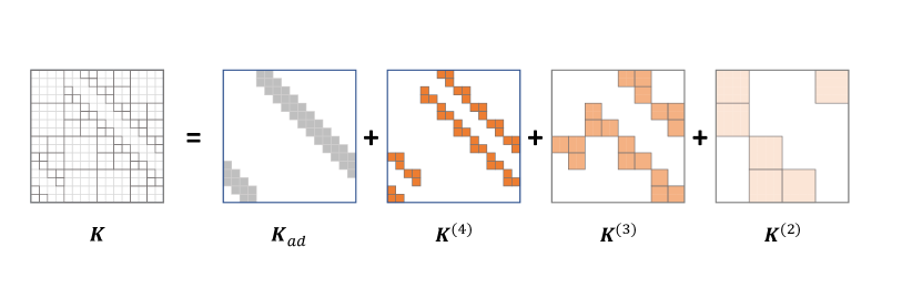
C.3 Adaptive algorithm for non-uniform particle distribution
In particle simulation tasks, if the distribution of particles is not approximately uniform, an adaptive hierarchical splitting can be employed. Let the smallest interparticle spacing be , where is the number of particles. Then, we can scale the mesh such that the interparticle distance is at least and the mesh size is . The added mesh sites are treated as zero-mass particles. The kernel matrix has size and the hierarchical splitting constructed on this mesh has levels. The entire block-encoding procedure presented in Section 4 applies, with only an extra factor of in the normalization factor and the required resources of the block-encoding. The optimality of the normalization factor of this adaptive block-encoding is harder to state precisely, since it depends on the distribution of particles which is not determined a priori.
C.4 Generalization of quantum hierarchical block-encoding
Here, we provide a block-encoding procedures in which one has direct access to the structure of the entry magnitudes, thus generalizing hierarchical block-encoding procedure presented in Section 4.1 and Section C.1.
First, we present a procedure for preparing a quantum state , where , with high probability of success. For any , let and . Also, let . Apart from the oracle , our procedure assumes the following oracle is provided:
| (47) |
where the first register is qubits and the second register is qubits, and is an efficiently computable and reversible function that computes the index of the -th element in the set (according to some fixed ordering, e.g. top to bottom if is treated as a column vector) if , or else the oracle writes as a bit string on the concatenation of the two registers (so that the first register will be non-zero). This ensures the oracle is reversible. An example of such efficient and reversible is in regular -matrix splitting. Our procedure is as follows:
| (query and rotate ancilla qubit) |
Above, we have ignored the terms when is invalid () in the sum because we can simply set for those cases. Furthermore, observe that the superposition has support on all indices. Thus, conditioning on the ancilla being zero, we obtain the desire state . The probability of successfully post-selecting is , where
| (48) |
We also assumed that the first operation in the procedure, which maps to a weighted superposition over , can be done perfectly. In fact, it can only be block-encoded with an extra normalization factor of : for a vector one can simply do
When including this step into the procedure above, the probability of successfully post-selecting and obtaining is .
Intuitively, our procedure exploits the structure of the amplitudes such that in the controlled rotation step, the ancilla has a large component in the good subspace .
The procedure to block-encode a matrix follows similarly. For simplicity, assume is Hermitian and . Let be the set of row indices of the entries in column whose values are in the range . Let , let . Let be such that . Our procedure, generalizing Section C.1, proceeds as follows:
The right part
For any column index :
| (49) | ||||
| (query and rotate ancilla qubit) |
Here, is similar to that in Equation 47; it returns the row index, , of the -th element in . We ignore the terms when is invalid () as we can set for those terms. Importantly, the above superposition has support over all row indices.
The left part
Similarly, we can construct a unitary that queries all the column indices
| (50) |
where is the column index of the -th element in .
Combining Equation 49 and Equation 50 we obtain a unitary that is block-encodes with a normalization factor of . If we take into consideration of first step Equation 49 (i.e. preparing ) as did in the quantum state preparation procedure above, then the normalization factor is . We now compare with the operator norm . If the entries of are real and non-negative, we have that
| (51) |
Thus, compared to the optimal block-encoding (one that has normalization factor equal to ), the presented block-encoding for is worse by at most a factor of . In other words, if , then the normalization factor is only a factor of worse than that of the optimal block-encoding. As before (section C.1), the numbers of elementary gates for the controlled rotation step and ancilla qubits are .
C.5 Condition number of polynomially and exponentially decaying kernels
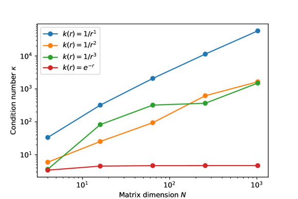
C.6 Kernels for which the naive block-encoding approach (Lemma 3.2) works optimally
We provide examples of kernels that are studied in classical -matrix or fast multipole method literature where the naive block-encoding approach of Lemma 3.2 (or Remark B.6) can be directly used to produce an optimal block-encoding of their kernel matrices.
The log kernel
The multiquadric kernel
(chapter 2.1, [13]). For this, let the kernel matrix be , where , . Directly applying Lemma 3.2 yields a using only additional resources. The operator norm of is bounded as , implying that the block-encoding is optimal.
We also list here, omitting the proofs, some typical kernels (which are not considered in classical -matrix) that can be optimally block-encoded by the naive approach of Lemma 3.2. For example, these include polynomially growing kernels and polyharmonic radial basis functions . Our numerical experiments indicate that these kernels are numerically low-rank, as shown in Figure 5. Furthermore, the first principal component (singular vector corresponding to the largest singular value) is close to uniform (the normalized all-ones vector). This explains why these kernels can be block-encoded by the naive block-encoding.
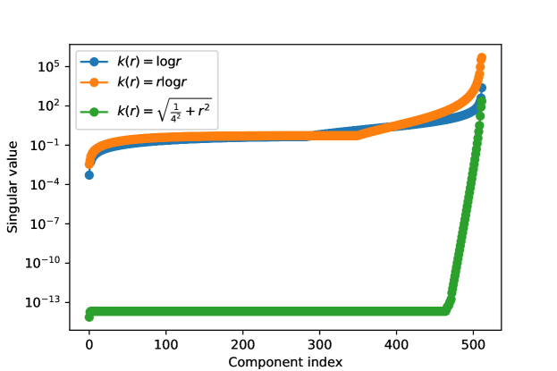
Appendix D Classical -matrices
D.1 Low-rank approximation using asymptotic smoothness
In this section, we show how the asymptotic smoothness condition (Equation 6) can be used to approximate an admissible block as a low-rank matrix. As a reminder, the asymptotic smoothness condition is
For instance, the log kernel directly holds this property.
Consider the admissible block , where . Let be the center of , we first obtain the -th order Taylor expansion of around
| (52) |
where the remainder can be bounded using the asymptotic smoothness property as follows
| (53) | ||||
Here, we have used the admissibility criteria (Definition 2.1) in the third inequality and that . Thus, can be approximated with exponentially small error by a rank- matrix
| (54) |
where , and
| (55) | |||
| (56) |
Next, we give an example of a kernel that does not directly satisfy the asymptotic smoothness condition (Equation 6), but can still be manipulated to apply the low-rank approximation. Consider the kernel . This kernel does not directly satisfy Equation 6. Nevertheless, for an admissible block at level , the kernel can be rewritten as
| (57) | ||||
where is the center of . In our setting (see Section 2), is simply the middle point of the corresponding segment on the domain . Furthermore, noting that , let
| (58) | ||||
and
| (59) |
Since is an admissible block (Definition 2.1), we have that . Therefore,
| (60) | ||||
Thus, can be approximated with error by the truncated sum in Equation 59 of order . Accordingly, the admissible block can be approximated to error by a rank- matrix.
D.2 Classical fast -matrix-vector multiplication
We count the number of operations needed to compute the matrix-vector multiplication, where and ,
| (61) |
The adjacent term is -sparse, hence requires only operations. In level , each block-row (row of blocks) requires computing 3 matrix-vector multiplications on dense matrices of size , which takes operations (where is the rank of the admissible blocks). There are block-rows, thus computing each requires operations. Since there are levels, the total operation complexity to compute all is . Adding up and costs another . As we have shown above, it is required that to achieve an error bound of on . Thus, the overall runtime of matrix-vector multiplication on -matrices is . We refer to [16] for operation complexities of other tasks on -matrices, such as matrix-matrix multiplication and matrix inversion, which are also when .
D.3 High dimensional hierarchical splittings
In the main text, we have seen that two key properties of the 1D hierarchical splitting that enables optimal quantum block-encodings were the logarithmic number of hierarchical levels and the block sparseness of each level (the third key property was that the off-diagonal entries were decaying or sufficiently smooth). Here, we show that these properties still hold for the 2D case and make a generalization argument for higher dimensional cases.
The 2D and 3D hierarchical splittings are well-studied in classical literature [17]. We will follow the indexing rules and conventions in the original work [17]. For an overview of hierarchical matrices and splittings, we suggest interested readers to read [13]–which covers the fast multipole algorithm (a special case of hierarchical splittings), [16]–which is the original paper that introduced the 1D hieararchical splitting, and [17]–the follow-up paper that generalized the hierarchical splittings to 2D and 3D problems.
Consider the uniform 2D grid of size and , where unit-mass particles are placed at sites (hence there are particles). We define the hierarchical partitions for this grid in the same spirit as Equation 3. For level , define the partitioning to be
| (62) |
where the clusters are
| (63) |
Before we proceed to construct the hierarchical splitting of the kernel matrix, we first have to decide how to number particles in a 2D grid. We follow the “canonical” choice in Section 4 of [17] (see Figure 6). In this numbering rule, the conversion from a grid site to the corresponding vectorized index is given by
| (64) |
where () is the binary representation of the row (column) index which ranges from to and is the CNOT function whose target bit is the second: , , , . The conversion from the vectorized index to grid site can be done by first writing in base- representation, then inverting the function . In summary, the entries of the kernel matrix are of the form
| (65) |
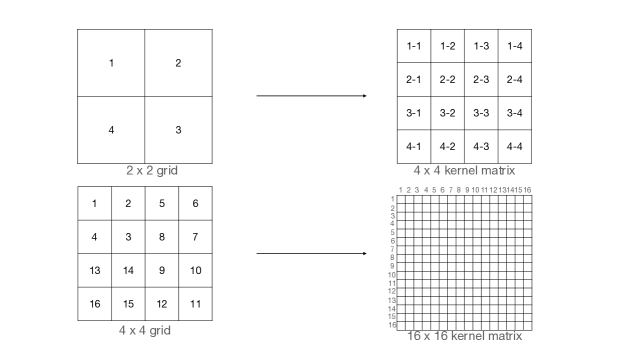
Next, we also need to define the admissibility criteria (Definition 2.1) for now 2D clusters. For two clusters in the same level, e.g., and , wee define their diameters to be the length of their diagonal, which are easily seen to be . Define the distance between these two clusters to be . We say the interactions between these two clusters are admissible if and only if
| (66) |
where we choose .
In other words, two clusters (hence the block in the kernel matrix that contains the interactions between them) are admissible when they are not neighboring along a column, row, or diagonal.
Having established the admissibility criteria, we proceed similarly to Section 2 to obtain the following decomposition of the kernel matrix
| (67) |
where contains the admissible interactions in level that have not been included in .
Next, we calculate the block-sparsity of by counting, among the clusters in level , how many clusters contribute to the potential at the particles inside a particular cluster . In fact, at most level- clusters need to be included. This can be most easily observed in Figure 7. Thus, the row-block-sparsity of is 27. And since is symmetric, the column-block-sparsity is also 27.
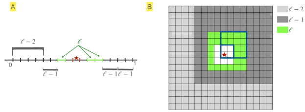
In summary, we still have hierarchical levels, each of which is block-sparse in the 2D case. Therefore, we can apply the entire block-encoding procedure in Section 4 to block-encode kernel matrices of a 2D grid. Below, we provide a similar analysis to that of Section 4.1 for polynomially decaying kernels (), showing that the hierarchical block-encoding is optimal for the 2D case.
At level (), an admissible matrix block , which contains the interactions between two clusters at level , has size ; and the minimum pairwise distance between particles within this block is by the definition of admissibility (Equation 66). It follows that the maximum entry in is . Thus, can be block-encoded by Lemma 3.2 with a normalization factor of . Then, can be block-encoded by Lemma 3.5 with a normalization factor of . The adjacent interaction part, , is a sparse matrix with sparsity and the largest entry equal to . Thus, can be block-encoded with a normalization factor of using Lemma B.5. Finally, the entire kernel matrix is obtained by summing over all levels using Lemma B.3. The overall normalization factor is
| (68) |
This block-encoding can be shown to be optimal by a similar method to Remark 4.1. We have that , where is the normalized all-ones vector. Furthermore, observe that
| (69) | ||||
In the limit , it can be easily verified that the above integral is when and when . Therefore, and the block-encoding procedure using hierarchical splitting is optimal.
Finally, the analysis in this section can be generalized to any -dimensional setting, where the block-sparsity of each hierarchical level is and the sparsity of the adjacent part is . For a visualization of 2D and 3D hierarchical splittings, see Figure 6 of [55], which has a smaller block-sparsity than the aforementioned value since diagonally neighboring clusters are considered admissible by the authors of [55], as opposed to our treatment in this section.
Appendix E Quantum state preparation for smooth functions
We provide an efficient procedure to prepare a quantum state whose entries are sampled from a smooth function. Consider a smooth function bounded by in the domain which can be approximated by a low-order Fourier series
| (70) |
where and the coefficients are .
We want to prepare the quantum state where the vector is
| (71) |
Let the QFT matrix be
| (72) |
Let , where at most terms are non-zero, and for .
Observe that
| (73) |
Since is sparse and the values and locations of the non-zero entries are known, one can easily prepare its quantum version with high probability using the following procedure.
-
1.
Prepare
-
2.
Call the oracle (where is a qubit string description of )
-
3.
Apply the conditioned rotation
-
4.
Uncompute and post-select on the subspace of the third register to obtain
Upon successfully obtaining (which happens with probability ), one applies the QFT to obtain . This procedure clearly applies for higher dimensional smooth functions. In these cases, one uses a tensor product of the conventional QFTs to transform the state back and forth between the real regime and the Fourier regime.
